dynamic programming optimal binary search tree...optimal binary search tree cole irma ben ann edna...

The complexity of different algorithms varies: O(n), Ω(n2), Θ(n·log2(n)), …

Různé algoritmy mají různou složitost: O(n), Ω(n2), Θ(n·log2(n)), …

Dynamic programming

Optimal binary search tree




IrmaColeCole

Ben

Ann EdnaEdna

FredFred JackJack

Ken MarkMark

HugoHugo

GeneGene

Nick

OrrieOrrie

0.05

DanaDana Lea

0.08

0.01

0.04

0.09

0.03

0.02 0.010.06 0.150.04 0.220.03 0.12

KeyQuery probability

0.05

Balanced but not optimal



FredFred

HugoHugo

GeneGene

0.05

DanaDana0.01

0.04

0.22 depth

2

1

3

4

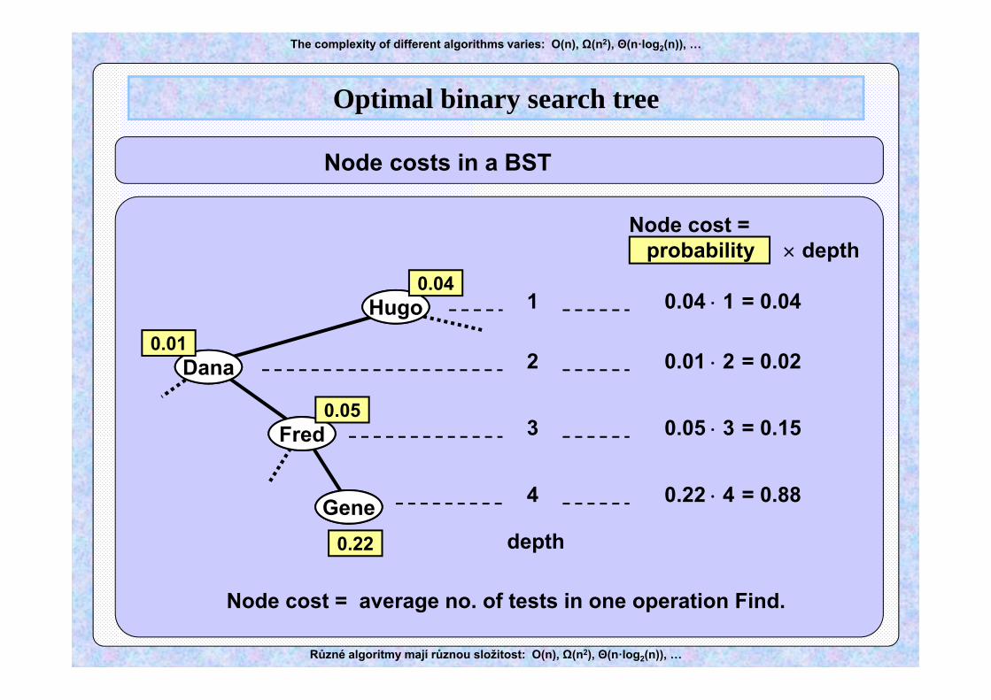
Node cost = average no. of tests in one operation Find.

0.04 1

0.01 2

0.05 3

0.22 4

= 0.04

= 0.02

= 0.15

= 0.88

Node cost = probability depth

Node costs in a BST


Θ(n·log2(n)), …


BenColeDanaEdnaFredGeneHugoIrma

Lea

JackKen

MarkNickOrrie

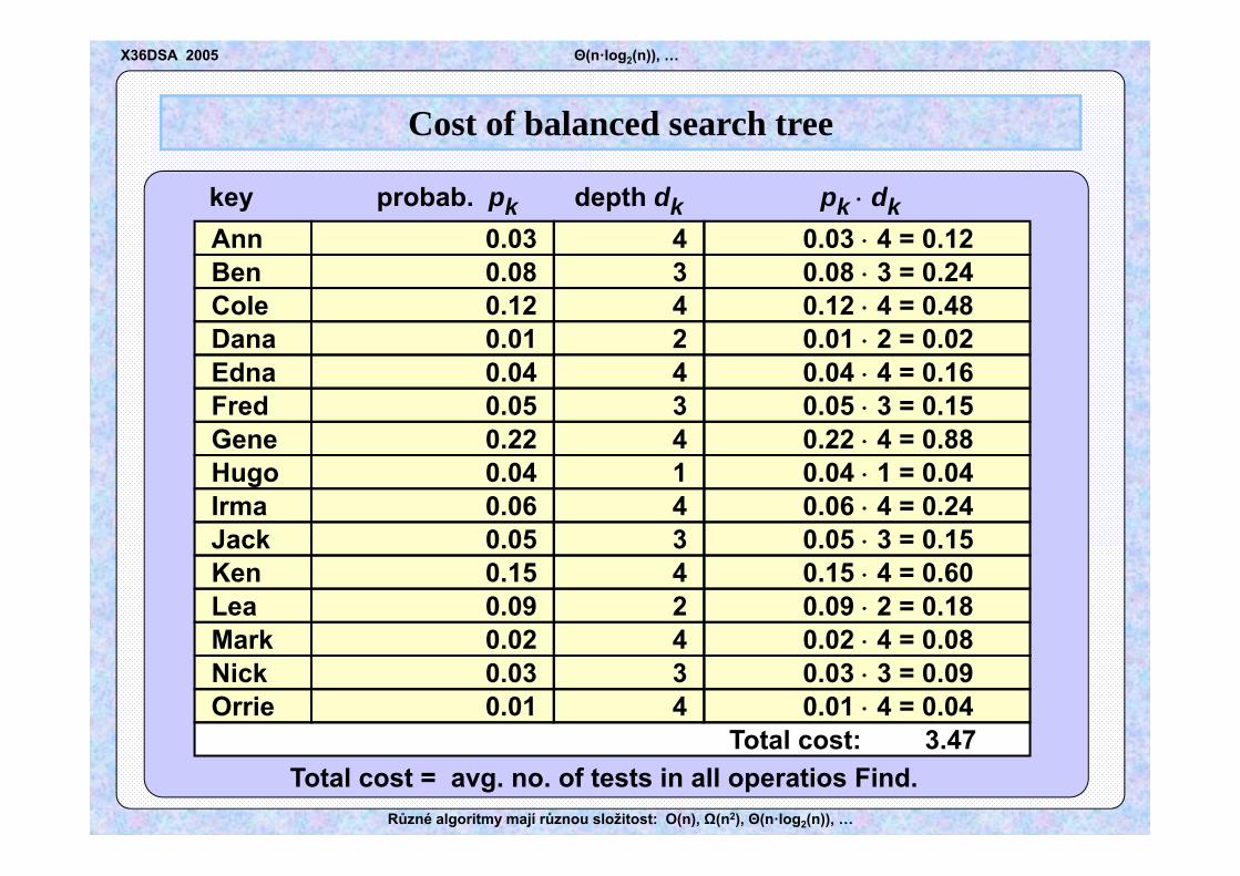
Annkey probab. pk depth dk pk dk

Total cost: 3.47

0.080.120.010.040.050.220.040.06

0.09

0.050.15

0.020.03

0.03

0.01

3 = 0.24 4 = 0.48 2 = 0.02 4 = 0.16 3 = 0.15 4 = 0.88 1 = 0.04 4 = 0.24

2 = 0.18

3 = 0.15 4 = 0.60

4 = 0.08 3 = 0.09

4 = 0.12

4 = 0.04

34243414

2

34

43

4

4

0.080.120.010.040.050.220.040.06

0.09

0.050.15

0.020.03

0.03

0.01

Total cost = avg. no. of tests in all operatios Find.

Cost of balanced search tree

X36DSA 2005



MarkMark0.02

OrrieOrrie

FredFred0.05

Ben0.08

DanaDana

HugoHugo

0.22

Lea

0.15

Nick

0.09

0.01

Irma

0.04

JackJack0.05

EdnaEdna0.04

GeneGene

Ann0.03

ColeCole

0.01

Ken

0.06

0.12

0.03

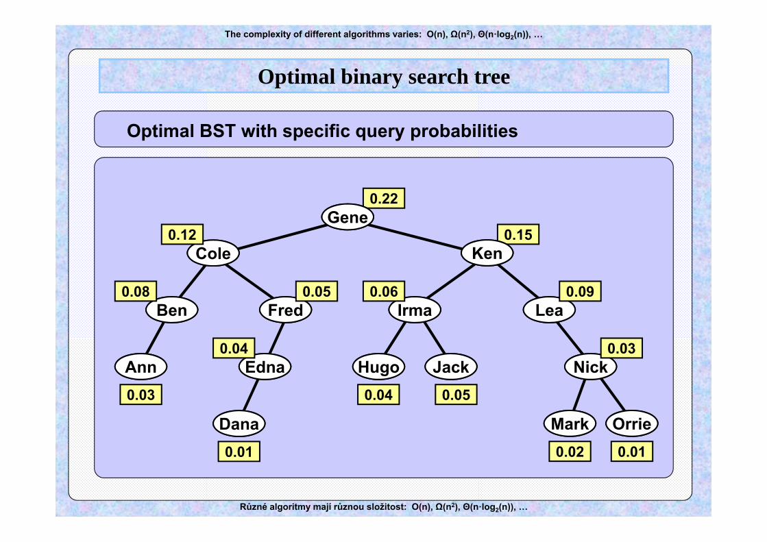
Optimal BST with specific query probabilities


Θ(n·log2(n)), …


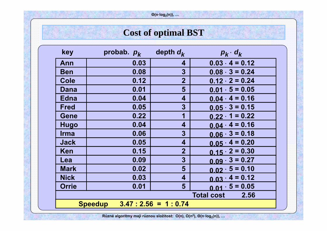
Cost of optimal BST

BenColeDanaEdnaFredGeneHugoIrma

Lea

JackKen

MarkNickOrrie

Annkey probab. pk depth dk pk dk

Total cost 2.56

0.080.120.010.040.050.220.040.06

0.09

0.050.15

0.020.03

0.03

0.01

3 = 0.24 2 = 0.24 5 = 0.05 4 = 0.16 3 = 0.15 1 = 0.22 4 = 0.16 3 = 0.18

3 = 0.27

4 = 0.20 2 = 0.30

5 = 0.10 4 = 0.12

4 = 0.12

5 = 0.05

32543143

3

42

54

4

5

0.080.120.010.040.050.220.040.06

0.09

0.050.15

0.020.03

0.03

0.01

Speedup 3.47 : 2.56 = 1 : 0.74



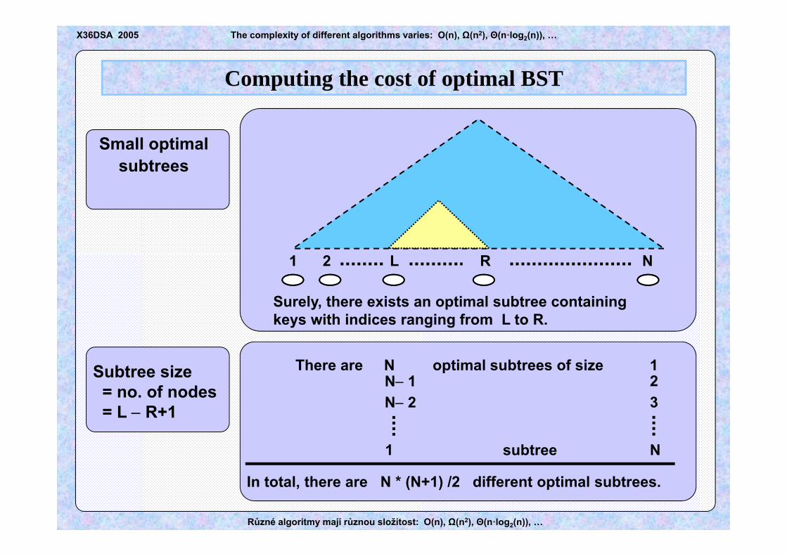
Computing the cost of optimal BST

Xyzpk

C2kC1k

k+1 RL k-1 k

cost of the left subtree of node kC1kcost of the right subtree of node kC2k

R

i=k+1picost = C1k + +

k-1i=L

pi + C2k + pk

pkRecursiveidea



1 2 L N R

Surely, there exists an optimal subtree containing keys with indices ranging from L to R.

There are N optimal subtrees of size 1

1 subtree N

2N 1N 2 3

In total, there are N * (N+1) /2 different optimal subtrees.

Subtree size = no. of nodes= L R+1

Small optimal subtrees

Computing the cost of optimal BST

X36DSA 2005



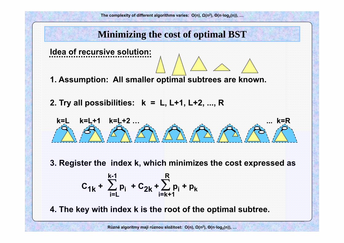
Minimizing the cost of optimal BST

2. Try all possibilities: k = L, L+1, L+2, ..., R

1. Assumption: All smaller optimal subtrees are known.

Idea of recursive solution:

3. Register the index k, which minimizes the cost expressed as R

i=k+1piC1k + +

k-1i=L

pi + C2k + pk

4. The key with index k is the root of the optimal subtree.

k=L k=L+1 k=L+2 … ... k=R



C(L,R) = min C(L, k-1) + i=L

k-1pi

i=k+1

Rpi+ C(k+1,R) +

L k R+ pk =

min C(L, k-1) + i=L

RpiC(k+1,R) +

L k R =

min C(L, k-1) + i=L

RpiC(k+1,R) +

L k R

=

=

C(L,R) ...... Cost of optimal subtree containig keys with indices:L, L+1, L+2, ..., R-1, R

The value minimizing (*) is the index of the root of the optimal subtree

(*)

Minimizing the cost of optimal BST

X36DSA 2005



Data structures for computing optimal BST

Costs of optimal subtrees

array C [L][R] (L ≤ R)

Roots of optimal subtrees

array roots [L][R] (L ≤ R)

L

R

0

1 2 3 4 N

3

12

N+1

L

R

0

3

12

N+1

L ≤ R L ≤ R

diagonal ... L= R diagonal ... L= R

X36DSA 2005



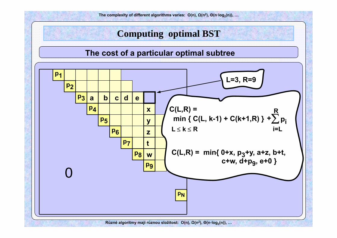
p5

p4

p3

p1

p6p7

p8p9

p2

pN

0

a b c d exyztw

L=3, R=9

i=L

Rpi+

L k R

C(L,R) = min C(L, k-1) + C(k+1,R)

C(L,R) = min 0+x, p3+y, a+z, b+t, c+w, d+p9, e+0

The cost of a particular optimal subtree

Computing optimal BST



Dynamic programming strategy – First process the smallest subtrees, then the bigger ones,

then still more bigger ones, etc...


Stop



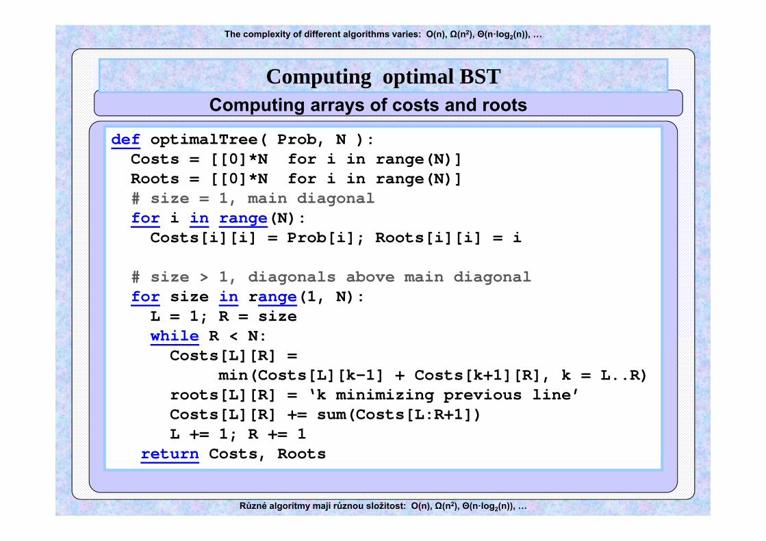
def optimalTree( Prob, N ):Costs = [[0]*N for i in range(N)] Roots = [[0]*N for i in range(N)]# size = 1, main diagonalfor i in range(N):Costs[i][i] = Prob[i]; Roots[i][i] = i

# size > 1, diagonals above main diagonal for size in range(1, N):L = 1; R = sizewhile R < N:Costs[L][R] =

min(Costs[L][k-1] + Costs[k+1][R], k = L..R)roots[L][R] = ‘k minimizing previous line’Costs[L][R] += sum(Costs[L:R+1]) L += 1; R += 1

return Costs, Roots

Computing arrays of costs and rootsComputing optimal BST



# standard BST insertdef buildTree( Tree, L, R, Roots, Nodes ):if R < L: returnrootindex = Roots[L][R]# standard BST insert# nodes in Nodes have to be sorted in increasing# order of their key valuesTree.insert( Nodes[rootindex].key ) buildTree( Tree, L, rootindex-1, Roots, Nodes )buildTree( Tree, rootindex+1, R, Roots, Nodes )

Building optimal BST using the array of subtree roots




0 1 2 3 3 3 3 3 7 7 7 7 7 7 7 70 0 2 3 3 3 3 7 7 7 7 7 7 7 7 70 0 0 3 3 3 3 7 7 7 7 7 7 7 7 70 0 0 0 4 5 6 7 7 7 7 7 7 7 7 70 0 0 0 0 5 6 7 7 7 7 7 7 7 7 70 0 0 0 0 0 6 7 7 7 7 7 7 7 11 110 0 0 0 0 0 0 7 7 7 7 7 11 11 11 110 0 0 0 0 0 0 0 8 9 9 11 11 11 11 110 0 0 0 0 0 0 0 0 9 9 11 11 11 11 110 0 0 0 0 0 0 0 0 0 10 11 11 11 11 110 0 0 0 0 0 0 0 0 0 0 11 11 11 11 110 0 0 0 0 0 0 0 0 0 0 0 12 12 12 120 0 0 0 0 0 0 0 0 0 0 0 0 13 14 140 0 0 0 0 0 0 0 0 0 0 0 0 0 14 140 0 0 0 0 0 0 0 0 0 0 0 0 0 0 150 0 0 0 0 0 0 0 0 0 0 0 0 0 0 0

Roots of optimal subtrees




0 1 2 3 3 3 3 3 7 7 7 7 7 7 7 70 0 2 3 3 3 3 7 7 7 7 7 7 7 7 70 0 0 3 3 3 3 7 7 7 7 7 7 7 7 70 0 0 0 4 5 6 7 7 7 7 7 7 7 7 70 0 0 0 0 5 6 7 7 7 7 7 7 7 7 70 0 0 0 0 0 6 7 7 7 7 7 7 7 11 110 0 0 0 0 0 0 7 7 7 7 7 11 11 11 110 0 0 0 0 0 0 0 8 9 9 11 11 11 11 110 0 0 0 0 0 0 0 0 9 9 11 11 11 11 110 0 0 0 0 0 0 0 0 0 10 11 11 11 11 110 0 0 0 0 0 0 0 0 0 0 11 11 11 11 110 0 0 0 0 0 0 0 0 0 0 0 12 12 12 120 0 0 0 0 0 0 0 0 0 0 0 0 13 14 140 0 0 0 0 0 0 0 0 0 0 0 0 0 14 140 0 0 0 0 0 0 0 0 0 0 0 0 0 0 150 0 0 0 0 0 0 0 0 0 0 0 0 0 0 0

Tree and array correspondence


MarkMark

0.02

OrrieOrrie

FredFred0.05

Ben0.08

DanaDana

HugoHugo

0.22

Lea

0.15

NickNick

0.09

0.01

IrmaIrma

0.04

JackJack

0.05

EdnaEdna0.04

GeneGene

Ann

0.03

ColeCole

0.01

Ken

0.06

0.12

0.03



1-A 2-B 3-C 4-D 5-E 6-F 7-G 8-H 9-I 10-J 11-K 12-L 13-M 14-N 15-O

1-A 0.03 0.14 0.37 0.39 0.48 0.63 1.17 1.26 1.42 1.57 2.02 2.29 2.37 2.51 2.562-B 0 0.08 0.28 0.30 0.39 0.54 1.06 1.14 1.30 1.45 1.90 2.17 2.25 2.39 2.443-C 0 0 0.12 0.14 0.23 0.38 0.82 0.90 1.06 1.21 1.66 1.93 2.01 2.15 2.204-D 0 0 0 0.01 0.06 0.16 0.48 0.56 0.72 0.87 1.32 1.59 1.67 1.81 1.865-E 0 0 0 0 0.04 0.13 0.44 0.52 0.68 0.83 1.28 1.55 1.63 1.77 1.826-F 0 0 0 0 0 0.05 0.32 0.40 0.56 0.71 1.16 1.43 1.51 1.63 1.677-G 0 0 0 0 0 0 0.22 0.30 0.46 0.61 1.06 1.31 1.37 1.48 1.528-H 0 0 0 0 0 0 0 0.04 0.14 0.24 0.54 0.72 0.78 0.89 0.939-I 0 0 0 0 0 0 0 0 0.06 0.16 0.42 0.60 0.66 0.77 0.81

10-J 0 0 0 0 0 0 0 0 0 0.05 0.25 0.43 0.49 0.60 0.6411-K 0 0 0 0 0 0 0 0 0 0 0.15 0.33 0.39 0.50 0.5412-L 0 0 0 0 0 0 0 0 0 0 0 0.09 0.13 0.21 0.2413-M 0 0 0 0 0 0 0 0 0 0 0 0 0.02 0.07 0.0914-N 0 0 0 0 0 0 0 0 0 0 0 0 0 0.03 0.0515-O 0 0 0 0 0 0 0 0 0 0 0 0 0 0 0.01

Costs of optimal subtrees




Dynamicprogramming

Longest commonsubsequence (LCS)



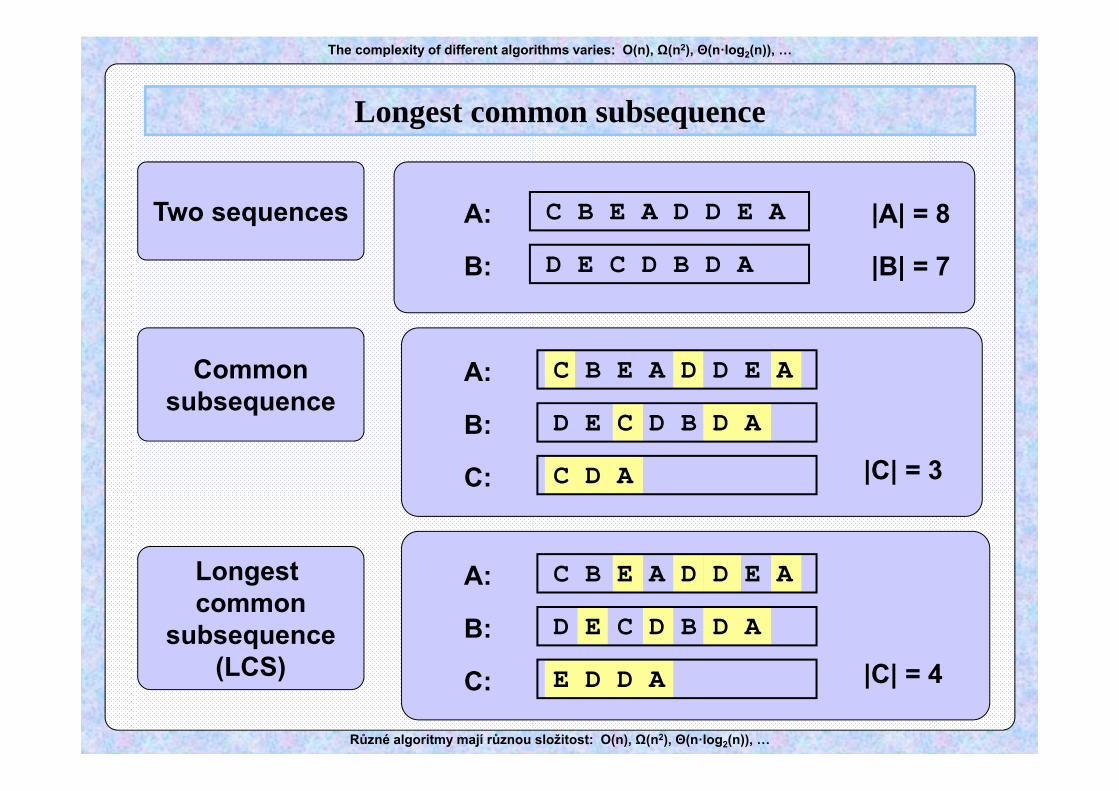
Longest common subsequence

C B E A D D E A

D E C D B D A

A:

B:

|A| = 8

|B| = 7

C B E A D D E A

D E C D B D A

A:

B:

C: C D A |C| = 3

C B E A D D E A

D E C D B D A

A:

B:

C: E D D A |C| = 4

Two sequences

Commonsubsequence

Longest common

subsequence(LCS)



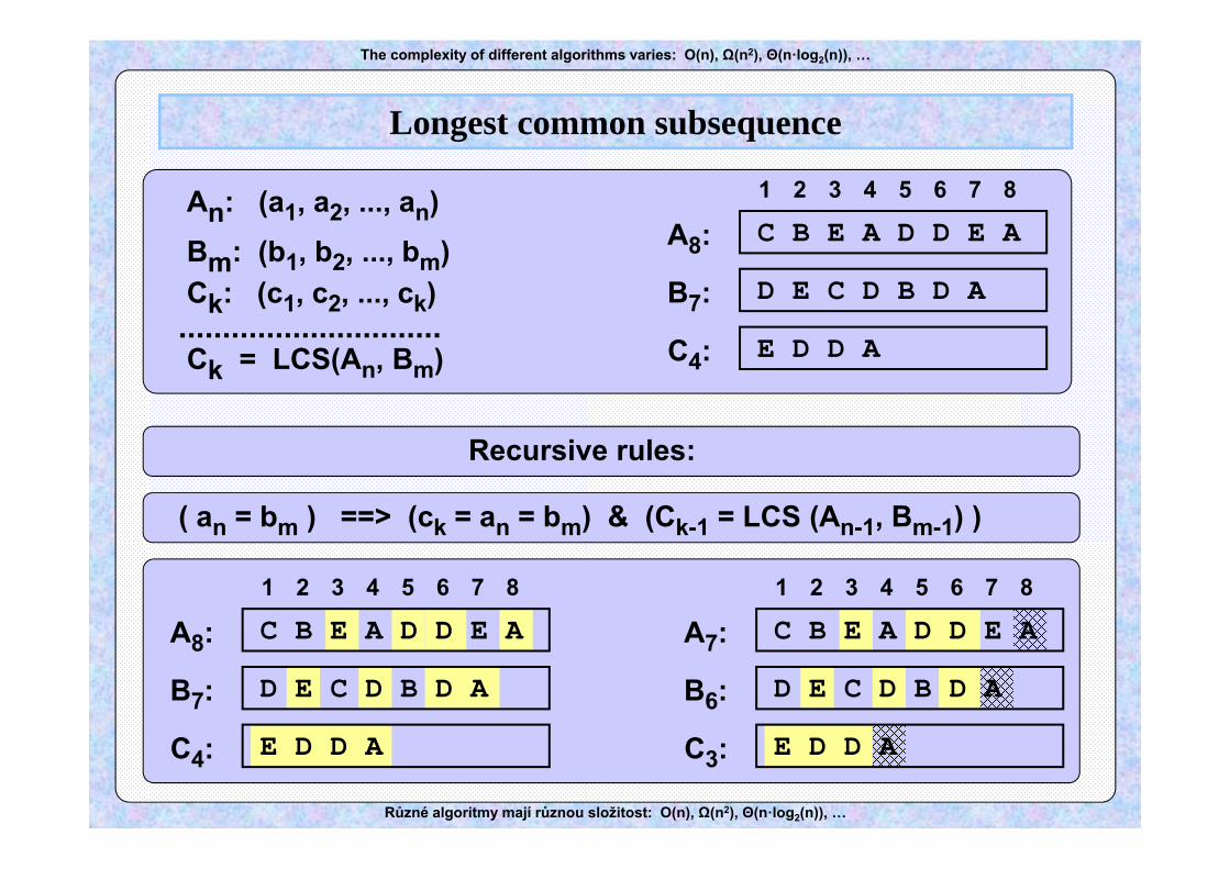
A8:

B7:

An: (a1, a2, ..., an)Bm: (b1, b2, ..., bm)Ck: (c1, c2, ..., ck)

1 2 83 4 5 6 7

C4:

Ck = LCS(An, Bm)

Recursive rules:

( an = bm ) ==> (ck = an = bm) & (Ck-1 = LCS (An-1, Bm-1) )

C B E A D D E A

D E C D B D A

A8:

B7:

1 2 83 4 5 6 7

C4: E D D A

C B E A D D E A

D E C D B D A

E D D A

A7:

B6:

1 2 83 4 5 6 7

C3:

C B E A D D E A

D E C D B D A

E D D A




( an != bm ) & (ck != an ) ==> (Ck = LCS (An-1, Bm) )

A7:

B6:

1 2 83 4 5 6 7

C3:

C B E A D D E

D E C D B D

E D D

A6:

B6:

1 2 83 4 5 6 7

C3:

C B E A D D E

D E C D B D

E D D

A5:

B5:

1 2 83 4 5 6 7

C2:

C B E A D

D E C D B

E D

A5:

B4:

1 2 83 4 5 6 7

C2:

C B E A D

D E C D B

E D

( an != bm ) & (ck != bm ) ==> (Ck = LCS (An, Bm-1) )




Recursive function c(m, n) computes LCS length

C(n,m) = 0

C(n-1, m-1) +1 n = 0 or m = 0 n > 0, m > 0, an = bm

n > 0, m > 0, an ≠ bmmax C(n-1, m), C(n, m-1)

Dynamic programming strategy

C[n][m]

n

m

for a in range( 1, n+1 ):for b in range( 1, m+1 ):

C[a][b] = ....




Construction of 2D LCS array

def findLCS(): for a in range( 1, n+1 ):for b in range( 1, m+1 ):if A[a] == B[b]:

C[a][b] = C[a-1][b-1]+1arrows[a][b] = DIAG

else: if C[a-1][b] > C[a][b-1]:

C[a][b] = C[a-1][b];arrows[a][b] = UP

else:C[a][b] = C[a][b-1];arrows[a][b] = LEFT




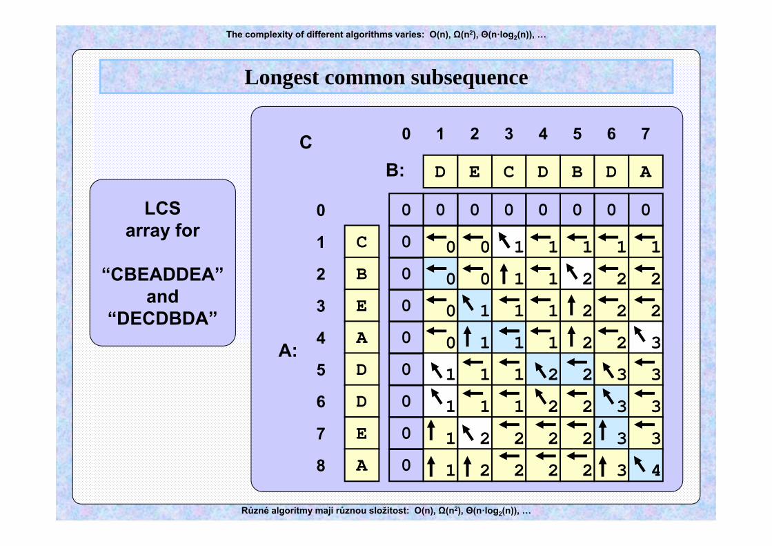
3 4 5 6 71 2

C

B

E

A

D

D

E

A

0

00

0

0

0

1

1

1

1

1

2

1

2

1

20

00

0

1

1

1

1

1

1

2

2

2

2

2

30

01

1

1

1

1

1

2

2

2

2

3

3

3

30

01

1

2

2

2

2

2

2

2

2

3

3

3

4

0 0 0 0 0 0 0 0

1

2

3

4

5

6

7

8

0

C D B D AD E

0C

A:

B:

LCSarray for

“CBEADDEA”and

“DECDBDA”




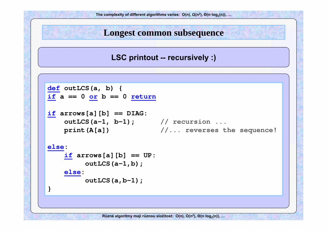
def outLCS(a, b) if a == 0 or b == 0 return

if arrows[a][b] == DIAG:outLCS(a-1, b-1); // recursion ...print(A[a]) //... reverses the sequence!

else:if arrows[a][b] == UP:

outLCS(a-1,b);else:

outLCS(a,b-1);

LSC printout -- recursively :)


dynamic programming optimal binary search tree...optimal binary search tree cole irma ben ann edna...

Documents