11

Earth System Modelsespecially those of

Intermediate Complexity

John ShepherdSchool of Ocean & Earth Science

Southampton Oceanography CentreUniversity of Southampton

Essential Earth System Processes(on land and sea, and in the air)

♦ Plate tectonics & volcanic activity♦ Weathering, erosion, sedimentation♦ Biological production, biogeochemistry and the carbon

cycle♦ Radiation (absorption, reflection, emission...)♦ Convection (mantle, atmosphere and ocean)♦ Oceanic transport (heat, salt, water, nutrients...)♦ Atmospheric transport (heat, water, CO2, etc)♦ Hydrology (evaporation, precipitation, run-off...)♦ Ice: accumulation, ablation, transport ♦ Soils & Sediments (formation & erosion)

22

EMICs : Earth (Climate) System Models(of intermediate complexity)

♦ What are they ?♦ Where are we now ?

• Examples• Overview

♦ Issues • Timescales, Structure & Purpose• Processes & Components• Dimensionality & Resolution• “Complexity”

♦ Where are we going ?♦ GENIE

Model types♦ Conceptual/illustrative

• to build & test general understanding• e.g. simplified box models

♦ experimental• to test mechanisms, evaluate processes, etc• to model general (not specific) system behaviour

♦ explanatory• to explain past events

• (fitted to some data, tested on the rest)

♦ simulation & prediction• as realistic as necessary/possible• for “operational” use

♦ N.B. The model is a working hypothesis

33

MIT Climate Modelling Initiative

Examples of ESM’s(not all EMICS !)

♦ Hadley Centre (HADCM3)• moderate resolution, 3D at 3.75° (atm) by 1.25° (ocean)

♦ MPI Hamburg (ECHAM/LSG)• 3D at 5.6°/5.6°

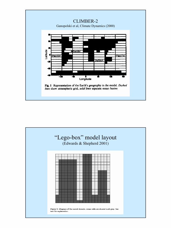
♦ Potsdam (CLIMBER-2)• 2.5D at 10° (lat) by 52° (long)

♦ Genie• 3D at 5° (lat) by 10° (long)

44

CLIMBER-2Ganopolski et al, Climate Dynamics (2000)

“Lego-box” model layout(Edwards & Shepherd 2001)

55

Reasons for wanting intermediate complexity (2D, 2.5D & 3D ) models

♦ to allow for spatial variation• include meridional transport of heat, water, etc ...

♦ to treat radiation (etc) explicitly• include vertical transports of heat, water, etc...

♦ need to represent both latitude & altitude• transport both by MMC and turbulence (eddies)

• (MMC = mean meridional circulation)

♦ also : heat & water transport by ocean • primarily due to meridional circulation

♦ Representation of continents & land surface…• The zonal dimension is also important !

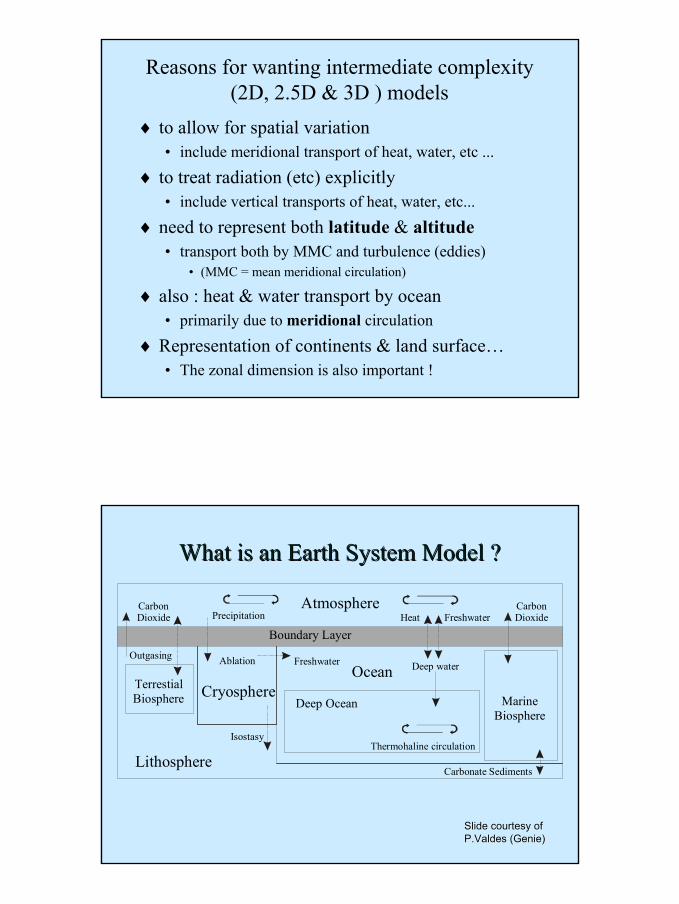
Atmosphere

Cryosphere

Boundary Layer

OceanTerrestialBiosphere Marine

Biosphere

Lithosphere

Freshwater

HeatPrecipitation

Thermohaline circulation

Ablation

Isostasy

Carbonate Sediments

CarbonDioxide

Deep Ocean

CarbonDioxide Freshwater

OutgasingDeep water

Slide courtesy of Slide courtesy of P.Valdes (Genie)P.Valdes (Genie)

What is an Earth System Model ?What is an Earth System Model ?

66

Components of an ESM(for the Climate System)

♦ Oceans♦ Atmosphere♦ Continents (configuration)♦ Land and sea surfaces (albedo)♦ Biosphere : marine and terrestrial vegetation♦ Cryosphere : ice sheets and sea-ice

Earth System ModelsProcesses & Timescales

Time-scale (years)

Planetary Continents Land Sea Atmosphere Ice Biosphere

Billions Solar evolution

Formation & Accretion

Erosion & deposition

Formation & Evolution

Formation & Oxygenation

Snowball Glaciations

??

Origin of Life, "Mostly

bacteria"~1e8 Continental

DriftColonisation

by plantsBasin

formationMostly warm

& ice-freePlants & animals

~1e7 Volcanic episodes

Mountain building

Sediment accumulation

Episodic Glaciations

Mass extinctions

Millions Crustal weathering

Chemistry (calcium)

Polar ice-caps

Species extinctions

~1e5 Insolation (Eccentricity)

Sea-level changes

Glacial cycles

~1e4 (Obliquity & precession)

Chemistry (phosphate)

Last glacial to Holocene

Thousands Solar Variations ?

Thermo-haline circulation

Millennial (DO) Oscillations

Eco-system evolution

~100 ditto Abrupt Climate Changes

~10 ditto O-A Coupled Modes?

Decadal Modes?

~1 Sea-ice variability

77

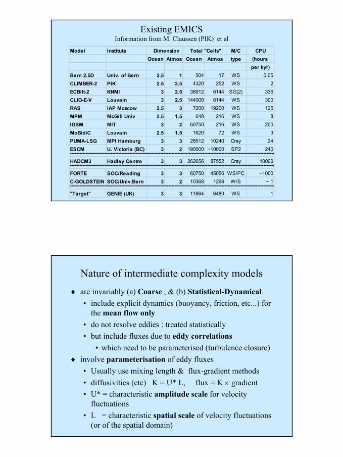
Existing EMICSInformation from M. Claussen (PIK) et al

Model Institute Dimension Total "Cells" M/C CPUOcean Atmos Ocean Atmos type (hours

per kyr)Bern 2.5D Univ. of Bern 2.5 1 504 17 WS 0.05CLIMBER-2 PIK 2.5 2.5 4320 252 WS 2ECBilt-2 KNMI 3 2.5 38912 6144 SG(2) 336CLIO-E-V Louvain 3 2.5 144000 6144 WS 300RAS IAP Moscow 2.5 3 7200 19200 WS 125MPM McGill Univ 2.5 1.5 648 216 WS 8IGSM MIT 3 2 60750 216 WS 200MoBidiC Louvain 2.5 1.5 1620 72 WS 3PUMA-LSG MPI Hamburg 3 3 28512 10240 Cray 24ESCM U. Victoria (BC) 3 2 190000 ~10000 SP2 240-----------------------------------------------------------------------------------------------------------------------------------HADCM3 Hadley Centre 3 3 262656 87552 Cray 10000-----------------------------------------------------------------------------------------------------------------------------------FORTE SOC/Reading 3 3 60750 45056 WS/PC ~1000C-GOLDSTEIN SOC/Univ.Bern 3 2 10368 1296 W/S ~ 1-----------------------------------------------------------------------------------------------------------------------------------"Target" GENIE (UK) 3 3 11664 6480 WS 1

Nature of intermediate complexity models♦ are invariably (a) Coarse , & (b) Statistical-Dynamical

• include explicit dynamics (buoyancy, friction, etc...) for the mean flow only

• do not resolve eddies : treated statistically• but include fluxes due to eddy correlations

• which need to be parameterised (turbulence closure)♦ involve parameterisation of eddy fluxes

• Usually use mixing length & flux-gradient methods • diffusivities (etc) K = U* L, flux = K × gradient• U* = characteristic amplitude scale for velocity

fluctuations• L = characteristic spatial scale of velocity fluctuations

(or of the spatial domain)

88

2 and 3D Atmospheric Models

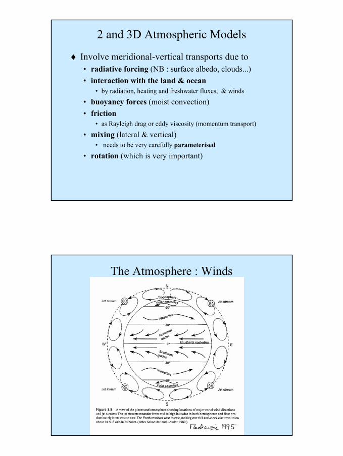
♦ Involve meridional-vertical transports due to• radiative forcing (NB : surface albedo, clouds...)• interaction with the land & ocean

• by radiation, heating and freshwater fluxes, & winds

• buoyancy forces (moist convection)• friction

• as Rayleigh drag or eddy viscosity (momentum transport)

• mixing (lateral & vertical)• needs to be very carefully parameterised

• rotation (which is very important)

The Atmosphere : Winds

99

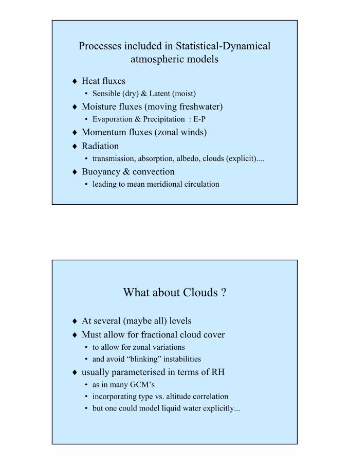
Processes included in Statistical-Dynamical atmospheric models

♦ Heat fluxes• Sensible (dry) & Latent (moist)

♦ Moisture fluxes (moving freshwater)• Evaporation & Precipitation : E-P

♦ Momentum fluxes (zonal winds)♦ Radiation

• transmission, absorption, albedo, clouds (explicit)....

♦ Buoyancy & convection• leading to mean meridional circulation

What about Clouds ?

♦ At several (maybe all) levels♦ Must allow for fractional cloud cover

• to allow for zonal variations• and avoid “blinking” instabilities

♦ usually parameterised in terms of RH• as in many GCM’s• incorporating type vs. altitude correlation• but one could model liquid water explicitly...

1010

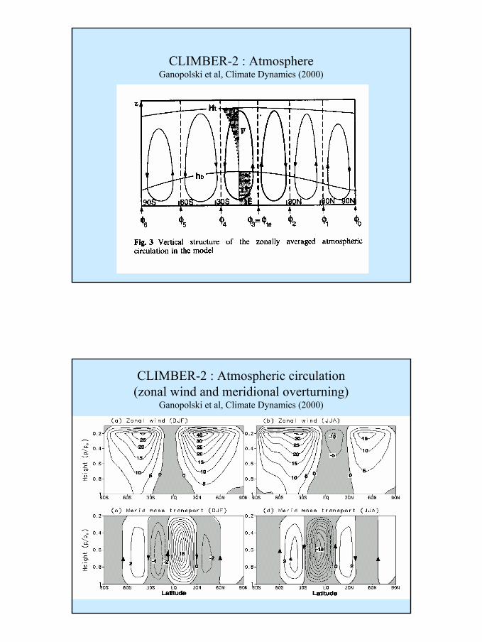
CLIMBER-2 : AtmosphereGanopolski et al, Climate Dynamics (2000)

CLIMBER-2 : Atmospheric circulation(zonal wind and meridional overturning)

Ganopolski et al, Climate Dynamics (2000)

1111

CLIMBER-2 : PrecipitationGanopolski et al, Climate Dynamics (2000)

2 and 2.5D Ocean ModelsInvolve meridional & vertical transports due to

• surface forcing (interaction with the atmosphere)• by radiation, heating and freshwater fluxes (and winds ?)

• and thus buoyancy forces• balancing friction

• as Rayleigh drag or eddy viscosity

• mixing (lateral & diapycnal) : usually specified• and effects of rotation (maybe, somehow)

♦ Examples include...• Stocker & Wright • Marotzke et al

1212

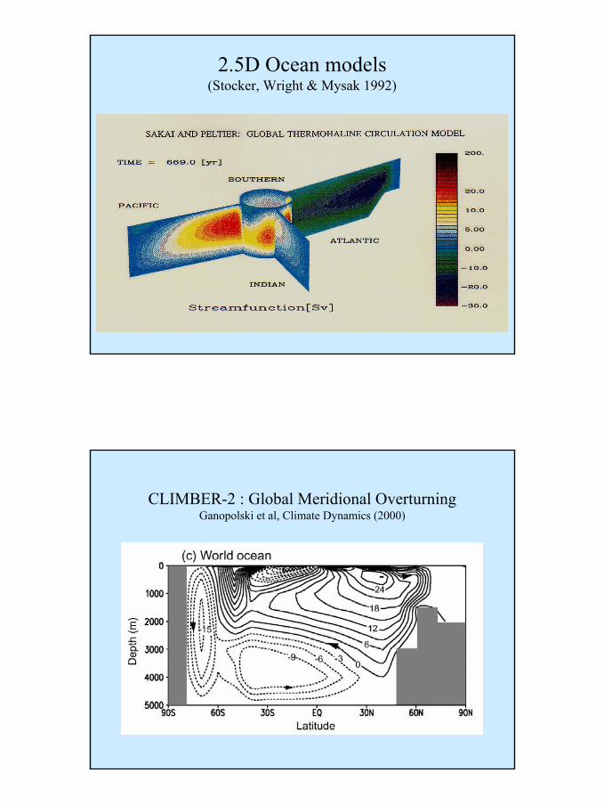
2.5D Ocean models(Stocker, Wright & Mysak 1992)

CLIMBER-2 : Global Meridional OverturningGanopolski et al, Climate Dynamics (2000)

1313

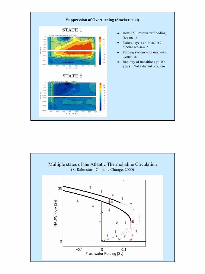
Suppression of Overturning (Stocker et al)

♦ How ??? Freshwater flooding (ice melt)

♦ Natural cycle : ~ bistable ? bipolar see-saw ?

♦ Forcing system with unknown dynamics

♦ Rapidity of transitions (<100 years): Not a distant problem

Multiple states of the Atlantic Thermohaline Circulation(S. Rahmstorf, Climatic Change, 2000)

1414

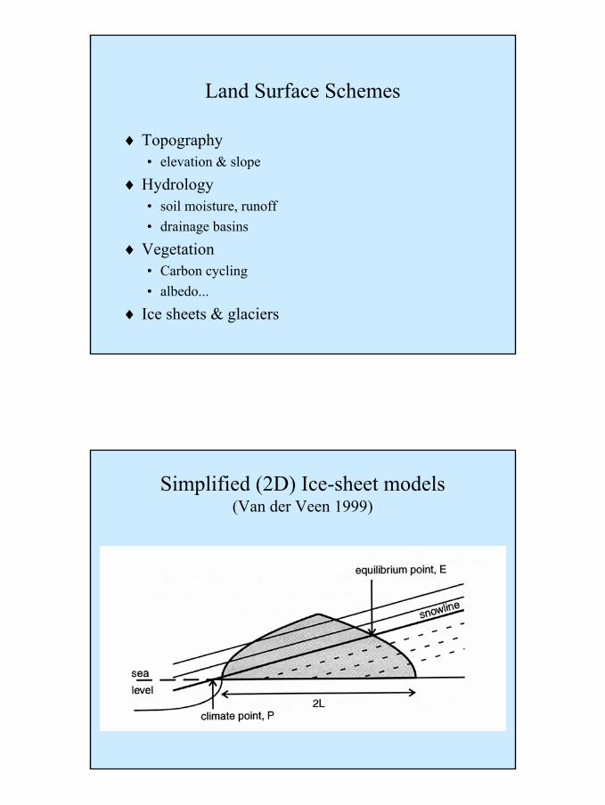
Land Surface Schemes

♦ Topography• elevation & slope

♦ Hydrology• soil moisture, runoff• drainage basins

♦ Vegetation• Carbon cycling• albedo...

♦ Ice sheets & glaciers

Simplified (2D) Ice-sheet models(Van der Veen 1999)

1515

Marine Biogeochemical Processes(after A. Ridgwell, 2001)

Why build yet another model ?♦ We need Fast & Efficient climate models

• To do long runs (over many centuries, up to and beyond 2100)• N.B. : 5,000 year time horizon for exhaustion of fossil fuels

and equilibration with marine sediments • To do many runs (to evaluate sensitivity & uncertainty

requires thousands of simulations) • To serve as the climate module for an Integrated

Assessment Model• (requires both of the above): many realisations

♦ Any climate model needs the Greenhouse Effect• ∆CO2 => ∆T : Climate Sensitivity

♦ To predict from emissions one needs a carbon cycle model (terrestrial and marine)• Emissions => ∆CO2 : (c.f. 1/3 : 1/3 : 1/3)

♦ We need to allow for surprises…• E.g. thermohaline shut-down

1616

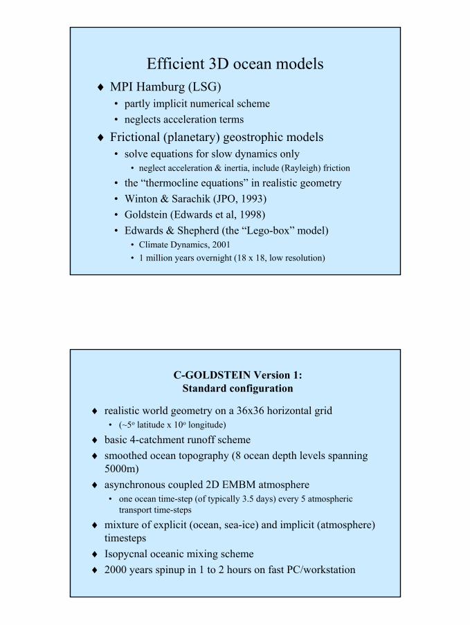
Efficient 3D ocean models♦ MPI Hamburg (LSG)

• partly implicit numerical scheme• neglects acceleration terms

♦ Frictional (planetary) geostrophic models• solve equations for slow dynamics only

• neglect acceleration & inertia, include (Rayleigh) friction

• the “thermocline equations” in realistic geometry• Winton & Sarachik (JPO, 1993)• Goldstein (Edwards et al, 1998)• Edwards & Shepherd (the “Lego-box” model)

• Climate Dynamics, 2001• 1 million years overnight (18 x 18, low resolution)

C-GOLDSTEIN Version 1:Standard configuration

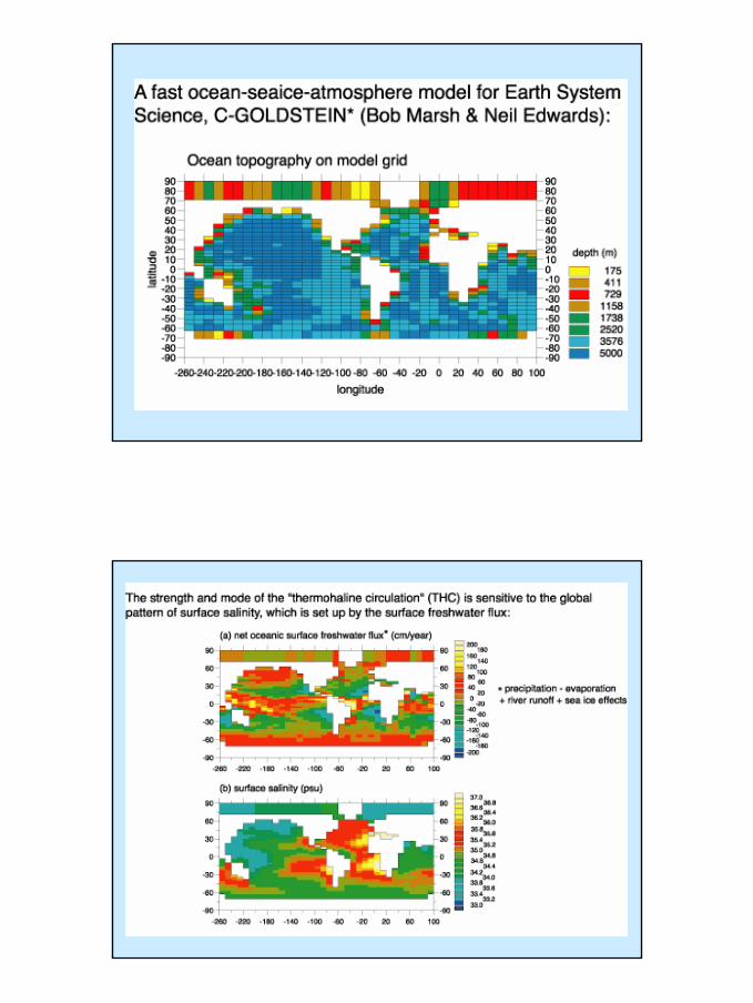
♦ realistic world geometry on a 36x36 horizontal grid • (~5o latitude x 10o longitude)

♦ basic 4-catchment runoff scheme♦ smoothed ocean topography (8 ocean depth levels spanning

5000m)♦ asynchronous coupled 2D EMBM atmosphere

• one ocean time-step (of typically 3.5 days) every 5 atmospherictransport time-steps

♦ mixture of explicit (ocean, sea-ice) and implicit (atmosphere)timesteps

♦ Isopycnal oceanic mixing scheme♦ 2000 years spinup in 1 to 2 hours on fast PC/workstation

1717

1818

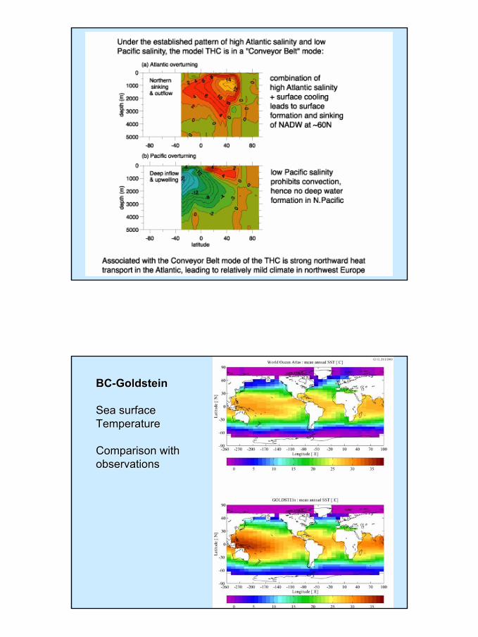
BCBC--Goldstein Goldstein

Sea surfaceSea surfaceTemperatureTemperature

Comparison withComparison withobservationsobservations

1919

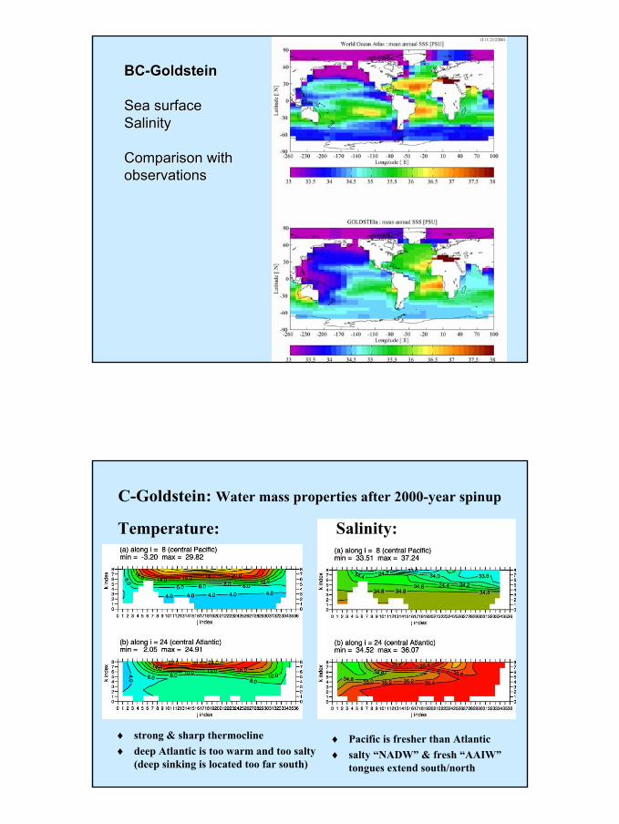
BCBC--Goldstein Goldstein

Sea surfaceSea surfaceSalinitySalinity

Comparison withComparison withobservationsobservations

C-Goldstein: Water mass properties after 2000-year spinup

Temperature: Salinity:

♦ strong & sharp thermocline♦ deep Atlantic is too warm and too salty

(deep sinking is located too far south)

♦ Pacific is fresher than Atlantic♦ salty “NADW” & fresh “AAIW”

tongues extend south/north

2020

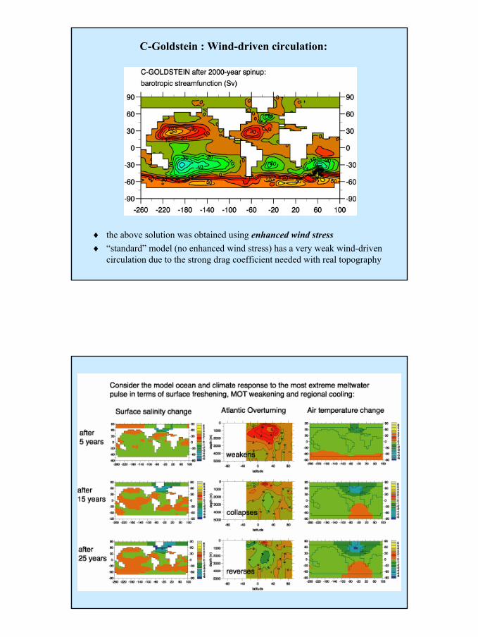
C-Goldstein : Wind-driven circulation:

♦ the above solution was obtained using enhanced wind stress♦ “standard” model (no enhanced wind stress) has a very weak wind-driven

circulation due to the strong drag coefficient needed with real topography

2121

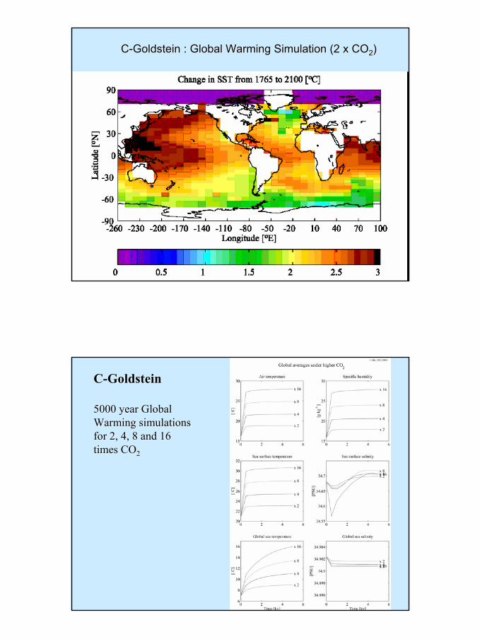
CC--Goldstein : Global Warming Simulation (2 x COGoldstein : Global Warming Simulation (2 x CO22))

CC--GoldsteinGoldstein

5000 year Global 5000 year Global Warming simulationsWarming simulationsfor 2, 4, 8 and 16for 2, 4, 8 and 16times COtimes CO22

2222

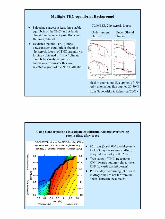
Multiple THC equilibria: Background

♦ Paleodata suggest at least three stableequilibria of the THC (and Atlantic climate) in the recent past: Holocene;Heinrich; Glacial

♦ Evidence that the THC “jumps” between such equilibria is found in “hysteresis loops” of THC strength vs. forcing - obtained in “slow” climate models by slowly varying an anomalous freshwater flux over selected regions of the North Atlantic

(from Ganopolski & Rahmstorf 2001)

Under presentclimate

Under Glacialclimate

CLIMBER-2 hysteresis loops:

black = anomalous flux applied 50-70oNred = anomalous flux applied 20-50oN

Using Condor pools to investigate equilibrium Atlantic overturning rate in dfwx-dfwy space

♦ 961 runs (3,844,000 model years!) took ~3 days, resolving at dfwx, dfwy intervals of just 0.02 Sv

♦ Two states of THC are apparent: ON (towards bottom right corner), OFF (towards top left corner)

♦ Present day overturning (at dfwx = 0, dfwy = 0) lies not far from the “cliff” between these states!

2323

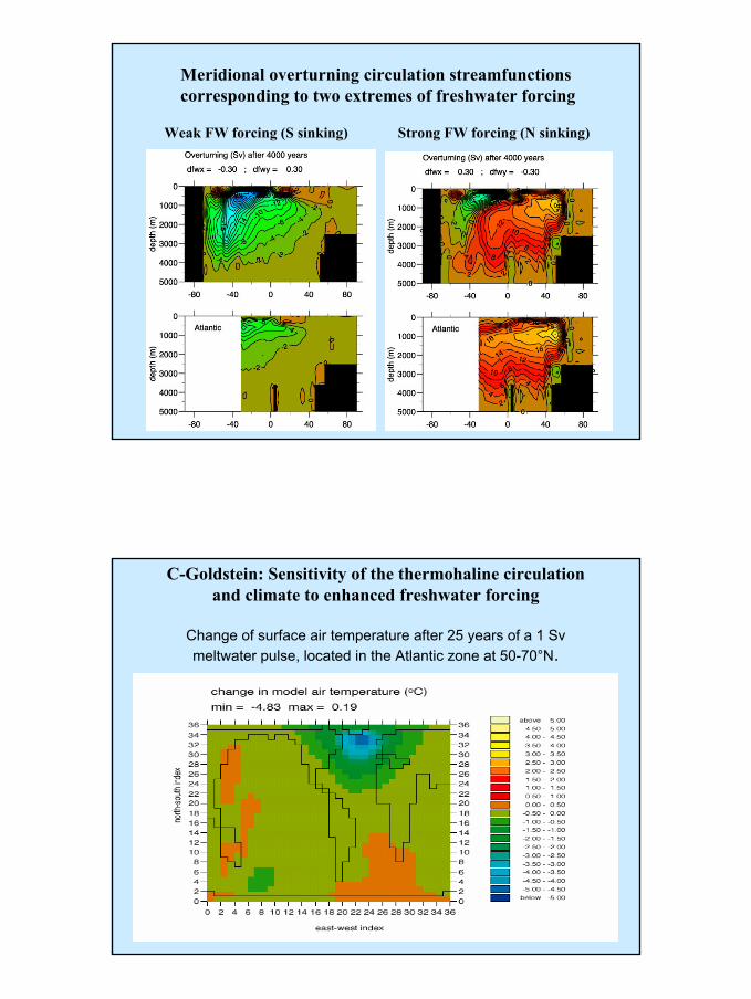
Meridional overturning circulation streamfunctionscorresponding to two extremes of freshwater forcing

Weak FW forcing (S sinking) Strong FW forcing (N sinking)

C-Goldstein: Sensitivity of the thermohaline circulation and climate to enhanced freshwater forcing

Change of surface air temperature after 25 years of a 1 Sv meltwater pulse, located in the Atlantic zone at 50-70°N.

2424

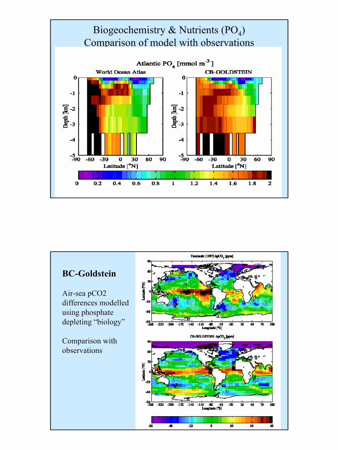
Biogeochemistry & Nutrients (PO4)Comparison of model with observations

BCBC--Goldstein Goldstein

AirAir--sea pCO2 sea pCO2 differences modelled differences modelled using phosphate using phosphate depleting depleting ““biologybiology””

Comparison withComparison withobservationsobservations

2525

Variability & Predictability♦ The Earth’s Climate System apparently exhibits

Multiple quasi-stable states• presumably due to positive feedbacks

♦ and Quasi-periodic behaviour• damped natural modes, paced by external forcing ?

♦ On all time scales (?) from seasons to aeons♦ We need efficient ESM’s

• to explore parameter-space• to run decent-sized ensembles, to establish variability,

and the extent of predictability• for proper interpretation of palaeo-climate proxies

♦ We need a diverse spectrum of efficient models, also to allow for inter-comparison & replication

Where next ? We need to...♦ Play !!

• to allow for accidental discoveries• this requires over-night runs (at most)

♦ run ensembles and/or explore parameter space• this needs hundreds to thousands of runs

♦ extend integration times to >30 kyr• with moderate resolution models

♦ ∴ develop faster schemes (with longer time-steps)♦ “populate the spectrum” of models

• in both structure & in resolution• inter-compare (up/down the spectrum)

♦ promote scalability and modularity♦ develop new & better parameterisations...

2626

Parameterisation

♦ is a high order intellectual activity♦ requires “asymptotic credibility”♦ preferably based on “sound science”♦ we could/should

• “cascade” parameterisations up/down the spectrum• use statistical representations of sub-grid scale

distributions• work with percentile values within cells • for hydrology, topography, clouds, ice, vegetation...

Conclusions♦ Earth System Models of Intermediate Complexity

• are necessary, desirable, and very useful tools• complementary to, and not “second best” to GCM’s

• are the only option (for the next decade or so)...• for testing our (seriously incomplete) understanding of

natural variations of climate• because these occur mainly on palaeo (multi-millennial

and longer) time-scales• EMIC’s are still at an early stage of development, and

are certainly capable of major improvement• We need more efficient representations of fluid

processes, and more effective parameterisations

♦ Eventually, we need to use data assimilation, and inverse modelling methods, on palaeo-datasets...

2727

Modelling & Philosophy

♦"Science may be described as the art of oversimplification: the art of discerning what we may with advantage omit."

• Karl Popper, “The Open Universe”, Hutchinson, London (1982)

“Man has lost the capacity to foresee and to forestall. He will end by destroying the Earth”

Albert Schweitzer, quoted by Rachel Carson, in her dedication of “Silent Spring”, (1962)