北大低温研・研究集会

干渉計解析の概要

百瀬宗武（茨城大理）

1

Interferometer in radio (1D): Each antenna obtains “E-field” information

V(D) is a Fourier component of T(δφ)→Image can be reconstructed by data from many baselines

when the delay is adjusted to the zenith ...

2

Cross correlation for δφ direction

|E(��)|2 exp

�+i2�

D

���

�

Integrating all the directions

V (D) =

�T (��) exp

�+i2�

D

���

�d(��)

Visibility and Brightness in 2D

3

Definition of “uv vector” for a projected baseline

(u, v)は地面，(x, y)は天球。u ∥ xは東西，v ∥ yは南北

�D = (Du, Dv) � �(u, v)

Fourier Transform between Visibility and Sky Brightness

V (u, v) =

��T (x, y)e+i2�(ux+vy) dxdy

T (x, y) =

��V (u, v)e�i2�(ux+vy) dudv

In reality, (1) antenna power pattern and (2) uv-sampling also affect the obtained data …

4

(1) V (u, v) � P (x, y)T (x, y)(パワーパターン) (真の輝度分布)(得られる

ビジビリティ)

where S(u, v) � B(x, y)

(2) P (x, y)Tdirty(x, y)

=

��[S(u, v)V (u, v)] e�i2�(ux+vy) dudv

= B(x, y) � [P (x, y)T (x, y)]

(直接出るマップ= Dirty Map)

(求めたい輝度分布)

(標本関数 or 重み関数)

(Dirty Beam)

※関数積のフーリエ変換 = 各関数のフーリエ変換の畳み込み

※パワーパターンは測定可能な量

Visibility vs. Image (from NAASC Memo #104)

5

ALMA Dirty Beam and Dirty Image

ALMA ES Proposal Preparation Tutorial Charlottesville, April 26, 2011 15

b(x,y) (dirty beam) B(u,v)

T(x,y) TD(x,y)

(dirty image)

B(x,y) S(u,v)

T(x,y)Dirty

Image

convolution

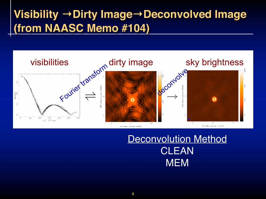
Visibility →Dirty Image→Deconvolved Image(from NAASC Memo #104)

6

ALMA From Visibilities to Images

ALMA ES Proposal Preparation Tutorial Charlottesville, April 26, 2011 29

•  Fourier transform of the measured V(u,v) to the image plane TD(x,y)

•  But difficult to do science on dirty image •  To determine (model of) T(x,y) we need to deconvolve b(x,y)

from TD(x,y) “clean” image

visibilities dirty image sky brightness

Deconvolution MethodCLEANMEM

Data Cube

7

Right Ascension

Declination

Vlos, or Frequency

T (x, y, �), or T (�, �, vlos)vlos is measured in “Local Standard of Rest” (LSR).

Channel Maps

8

Right Ascension

Declination

PV Diagram

9

Right Ascension

Declination

Vlos, or Frequency

PV Diagram

10

Right Ascension

Declination

Vlos, or Frequency

PV Diagram

11

Right Ascension

Declination

Vlos, or Frequency

PV Diagram

12

Right Ascension

Declination

Vlos, or Frequency

Moment Maps

13

※ 以下はすべて場所(α, δ)ごとで計算

積分強度

平均速度

速度分散 局所的なもの (乱流・熱速度)

+ ビーム内速度勾配

0th: I ��

T (v)dv

1st: vlos ��

v · T (v)dv

I

2nd: �v ���

(v � vlos)2 · T (v)dv

I

=

��v2 · T (v)dv

I� vlos.

Examples: HD142527 in 13CO (J=3-2)Briggs Wt (upper) and Uniform Wt (lower)

14

0th 1st 2nd

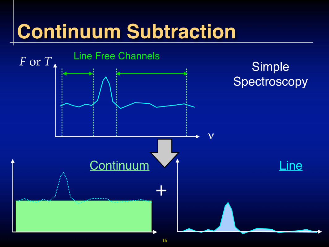
Continuum Subtraction

15

ν

F or T Simple Spectroscopy

Line Free Channels

+Continuum Line

Continuum Subtraction

16

ν

Real partor

Imag. part

Complex VisibilityLine Free Channels

+Continuum Line

Vector Averaging inline free channels

Residual

Cont. Visibility

LineVisibility

Peak Tb map of 13CO (J=3-2) around HD142527: Line only and Cont. added

17(1) 13CO, C18O が、少なくとも北側の明るい領域では両方とも光学的に厚く、密度でなく温度情報を与えていることを示す。（アバンダンス比だけでは不十分かもしれないので、optically thick surfaces をそれぞれトレースしていると考えるのが自然であることを述べる。）(2) 13CO ピーク強度を提示。連続波の加算が必要であること、最大で 36 K,方位角方向にほぼ一様であることを述べる。

10

13CO peak intensity map

67

… in different color code

Continuum in grey lines

Advanced Materials

18

CLEAN Algorithm

19

Start / Resume

放射ピーク ICC(x,y) を見出す

I(x,y)*B(x,y) を引く

ICC(x,y) を記録

Residualに拾うべきピークある？

A list of ICC(x,y)(Clean Components)

CLEAN beam BCL(x,y)

[Σ ICC(x,y)*BCL(x,y)]

+ R(x,y)

Residual Map R(x,y)

Dirty Map ID(x,y)

Final Image IFIN(x,y)

Yes

No

Operation Flow

Data Input/Output

Data Reduction in the case of Fukagawa et al. (2013)

20

ContinuumVisibility Model

Image

Gain Solution

Final Continuum

Image

LineVisibility

(cont-subtracted)

Final Line

Images

(cont-subtracted)

Raw Data

Calib. Data Final Gain

Solution

Flux Scale(Titan & Neptune)

Bandpass (3C279 & J1924-242)

Gain Table (J1427-4206)

SELF-CALx 6 Phase only

↓x 1 Amp & Phase

CLEAN

CLEAN (Uniform Wt)

CLEAN (Uniform Wt)

Self-Calibration: “Before-After”HD142527 Continuum @ 330 GHz

21

Before Self-Cal.

after1 iteration

solving phase only

Final Image6 iterations

solving phase +1 iteration

solving amp. & phase

※ 少しずつ慎重に（やり過ぎると1箇所に放射を集める場合あり）※ 独立した偏波成分を取得する受信機同士でconsistentな解を示しているか

rms = 2.24 mJy/beam 0.68 mJy/beam 0.13 mJy/beam

(理想は熱雑音のみで計算される値と一致すること)

Self-Calibration

22

明るくコンパクト 瞬時瞬時のVisibility Phaseを

支配。予測可能。

Nant < Nbaseline↓

アンテナベースの位相誤差

(大気水蒸気の揺らぎ，装置の位相揺らぎ等)を解くことができる

（モデルイメージの解との比較）

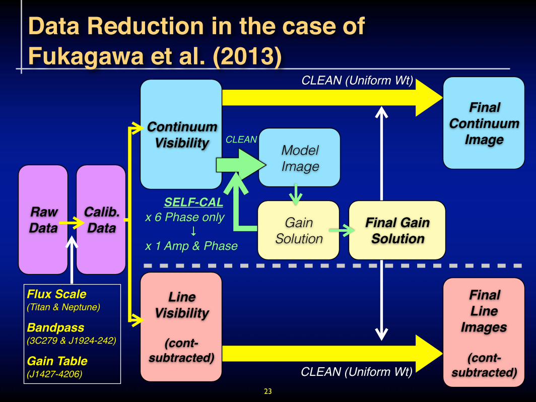
Data Reduction in the case of Fukagawa et al. (2013)

23

ContinuumVisibility Model

Image

Gain Solution

Final Continuum

Image

LineVisibility

(cont-subtracted)

Final Line

Images

(cont-subtracted)

Raw Data

Calib. Data Final Gain

Solution

Flux Scale(Titan & Neptune)

Bandpass (3C279 & J1924-242)

Gain Table (J1427-4206)

SELF-CALx 6 Phase only

↓x 1 Amp & Phase

CLEAN

CLEAN (Uniform Wt)

CLEAN (Uniform Wt)

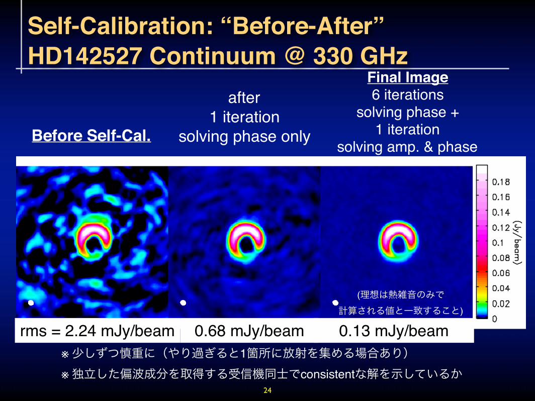
Self-Calibration: “Before-After”HD142527 Continuum @ 330 GHz

24

Before Self-Cal.

after1 iteration

solving phase only

Final Image6 iterations

solving phase +1 iteration

solving amp. & phase

※ 少しずつ慎重に（やり過ぎると1箇所に放射を集める場合あり）※ 独立した偏波成分を取得する受信機同士でconsistentな解を示しているか

rms = 2.24 mJy/beam 0.68 mJy/beam 0.13 mJy/beam

(理想は熱雑音のみで計算される値と一致すること)