efficiency at the maximum power output for simple two-level heat engine
TRANSCRIPT
Efficiency at the maximum power output for simple two-level heat engine
Sang Hoon Lee (이상훈) Statistical Physics Group, School of Physics, Korea Institute for Advanced Study [Rm 1437]
http://newton.kias.re.kr/~lshlj82
in collaboration with Jaegon Um (CCSS, CTP and Department of Physics and Astronomy, SNU) and Hyunggyu Park (School of Physics & Quantum Universe Center, KIAS)
KIAS School of Physics Workshop, 7 October, 2016 @ Phoenix Island, Jeju Island
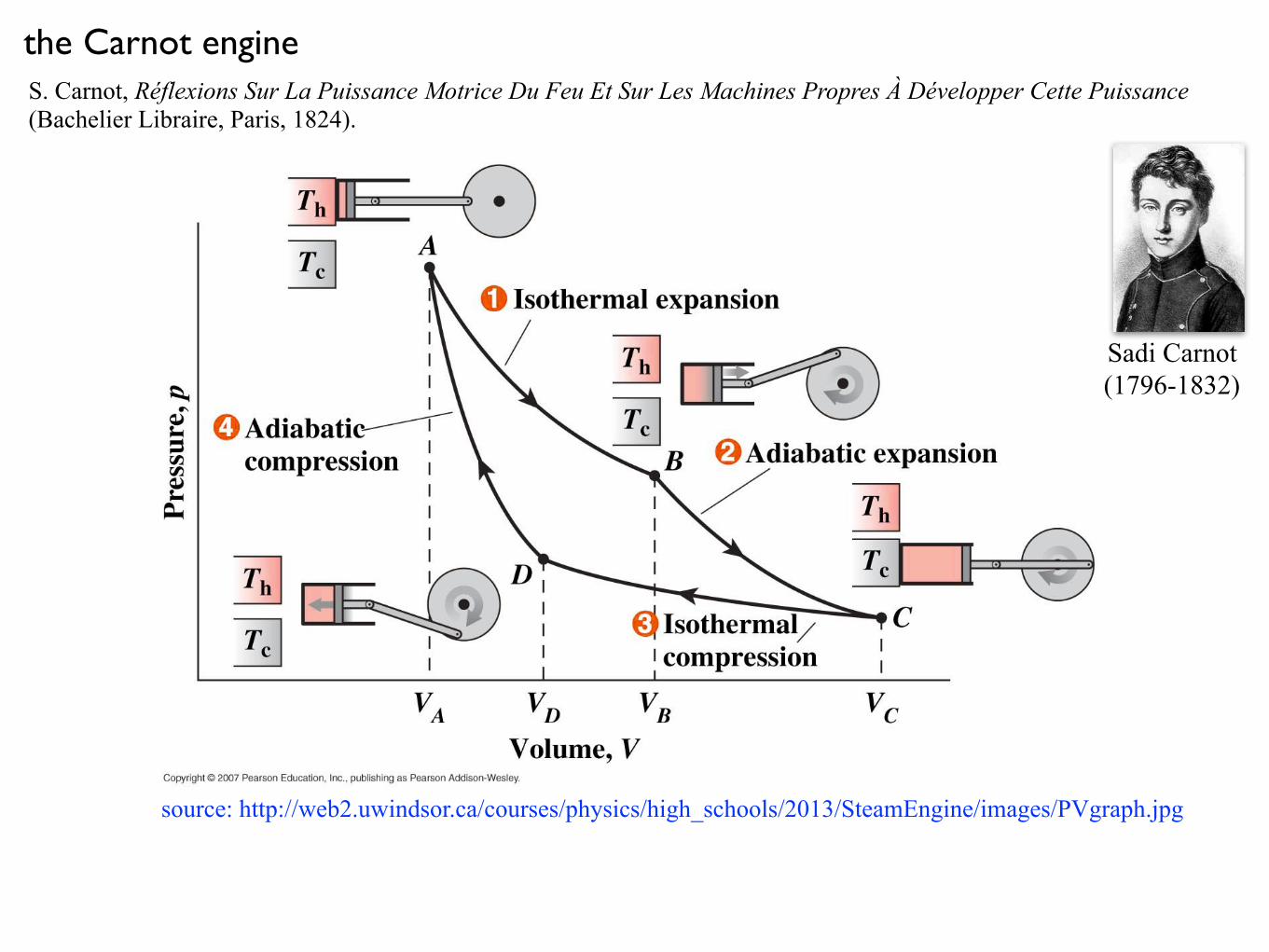
Carnot engine
source: http://web2.uwindsor.ca/courses/physics/high_schools/2013/SteamEngine/images/PVgraph.jpg
S. Carnot, Réflexions Sur La Puissance Motrice Du Feu Et Sur Les Machines Propres À Développer Cette Puissance (Bachelier Libraire, Paris, 1824).
the
Sadi Carnot (1796-1832)
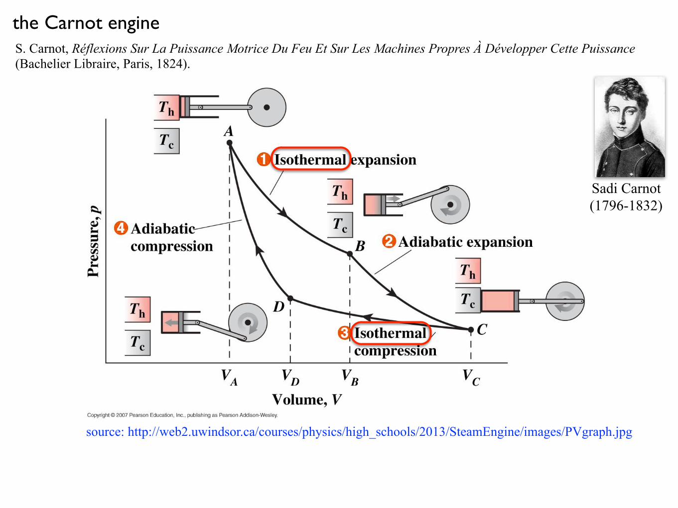
Carnot engine
source: http://web2.uwindsor.ca/courses/physics/high_schools/2013/SteamEngine/images/PVgraph.jpg
S. Carnot, Réflexions Sur La Puissance Motrice Du Feu Et Sur Les Machines Propres À Développer Cette Puissance (Bachelier Libraire, Paris, 1824).
the
Sadi Carnot (1796-1832)
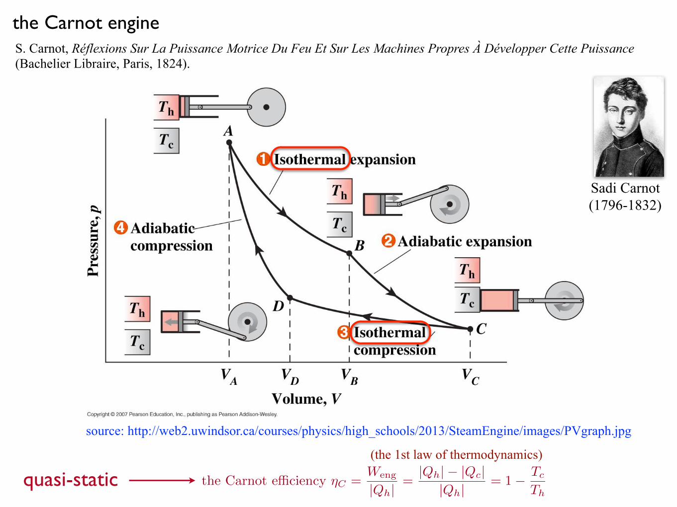
Carnot engine
source: http://web2.uwindsor.ca/courses/physics/high_schools/2013/SteamEngine/images/PVgraph.jpg
S. Carnot, Réflexions Sur La Puissance Motrice Du Feu Et Sur Les Machines Propres À Développer Cette Puissance (Bachelier Libraire, Paris, 1824).
the
Sadi Carnot (1796-1832)
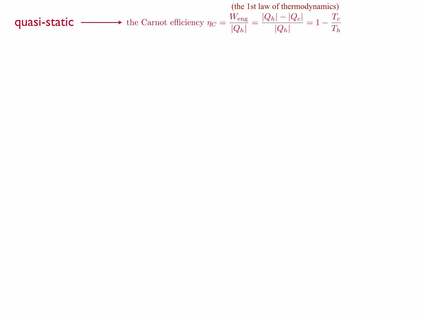
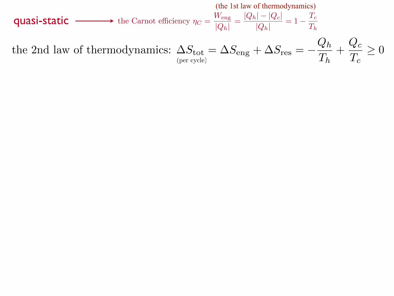
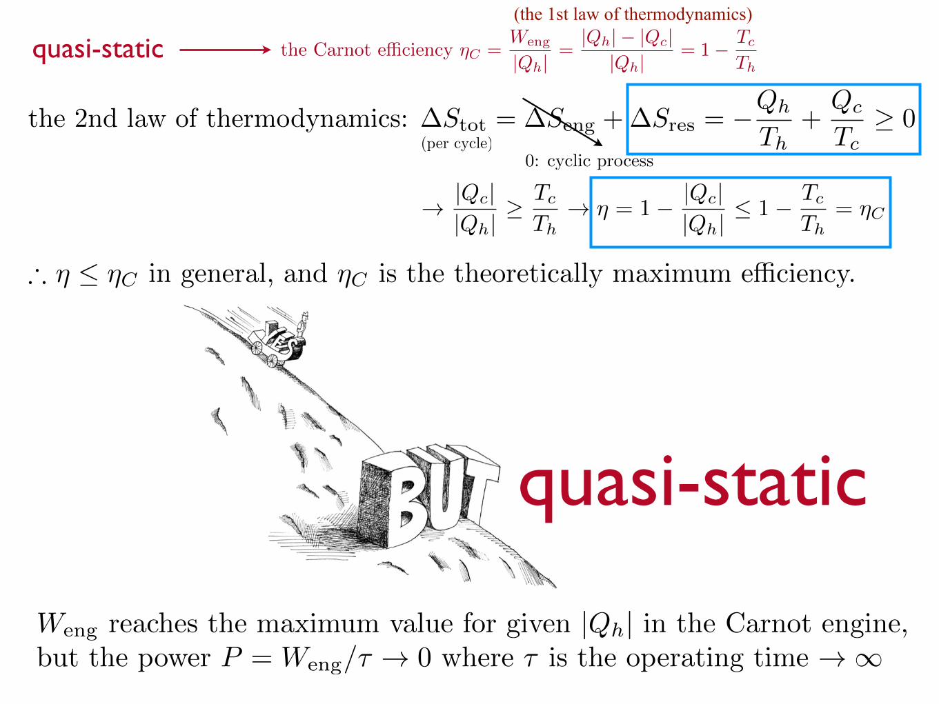
the Carnot e�ciency ⌘C =
Weng
|Qh|=
|Qh|� |Qc||Qh|
= 1� Tc
Thquasi-static
(the 1st law of thermodynamics)
the Carnot e�ciency ⌘C =
Weng
|Qh|=
|Qh|� |Qc||Qh|
= 1� Tc
Thquasi-static
(the 1st law of thermodynamics)
the Carnot e�ciency ⌘C =
Weng
|Qh|=
|Qh|� |Qc||Qh|
= 1� Tc
Thquasi-static
(the 1st law of thermodynamics)
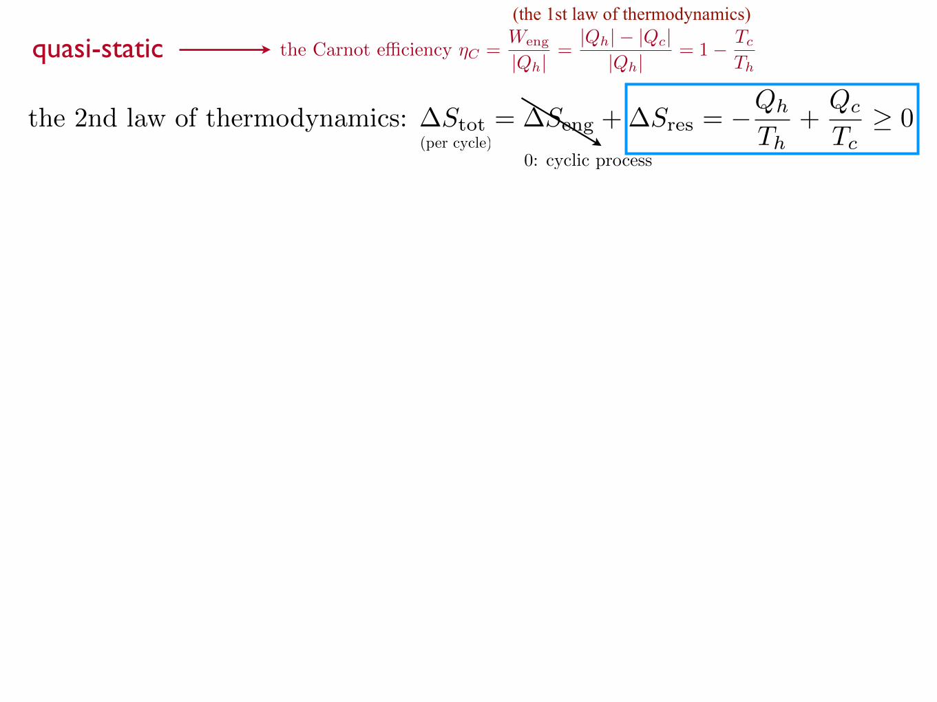
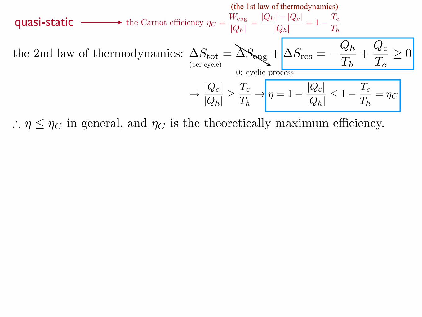
the 2nd law of thermodynamics: �Stot
= �Seng
+�Sres
= �Qh
Th+
Qc
Tc� 0
(per cycle)
the Carnot e�ciency ⌘C =
Weng
|Qh|=
|Qh|� |Qc||Qh|
= 1� Tc
Thquasi-static
(the 1st law of thermodynamics)
0: cyclic process
the 2nd law of thermodynamics: �Stot
= �Seng
+�Sres
= �Qh
Th+
Qc
Tc� 0
(per cycle)
the Carnot e�ciency ⌘C =
Weng
|Qh|=
|Qh|� |Qc||Qh|
= 1� Tc
Thquasi-static
(the 1st law of thermodynamics)
0: cyclic process
the 2nd law of thermodynamics: �Stot
= �Seng
+�Sres
= �Qh
Th+
Qc
Tc� 0
(per cycle)
! |Qc||Qh|
� Tc
Th! ⌘ = 1� |Qc|
|Qh| 1� Tc
Th= ⌘C
) ⌘ ⌘C in general, and ⌘C is the theoretically maximum e�ciency.
Weng reaches the maximum value for given |Qh| in the Carnot engine,
but the power P = Weng/⌧ ! 0 where ⌧ is the operating time ! 1
quasi-static
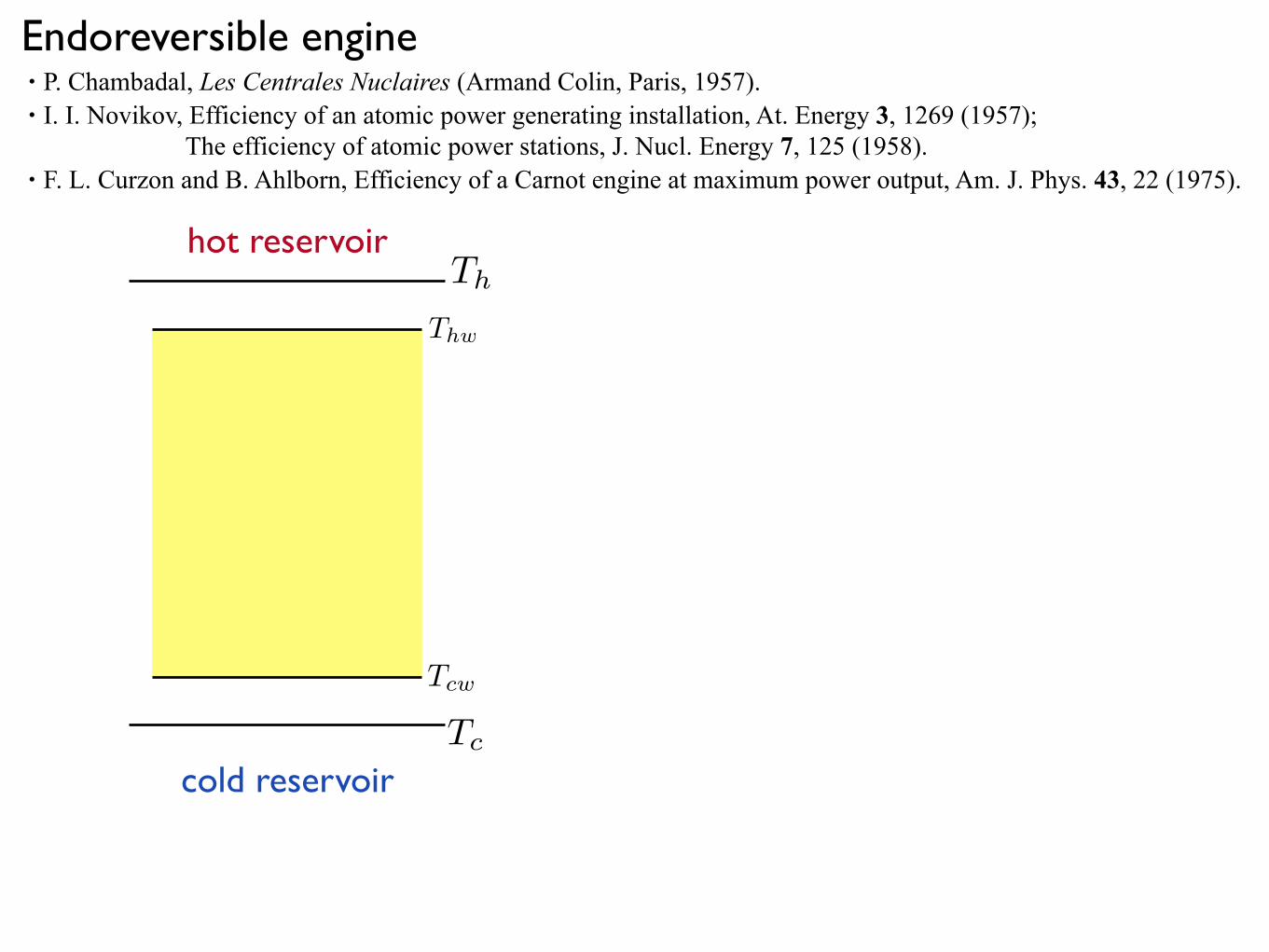
Th
Tc
hot reservoir
cold reservoir
Thw
Tcw
Endoreversible engine• P. Chambadal, Les Centrales Nuclaires (Armand Colin, Paris, 1957). • I. I. Novikov, Efficiency of an atomic power generating installation, At. Energy 3, 1269 (1957);
The efficiency of atomic power stations, J. Nucl. Energy 7, 125 (1958). • F. L. Curzon and B. Ahlborn, Efficiency of a Carnot engine at maximum power output, Am. J. Phys. 43, 22 (1975).
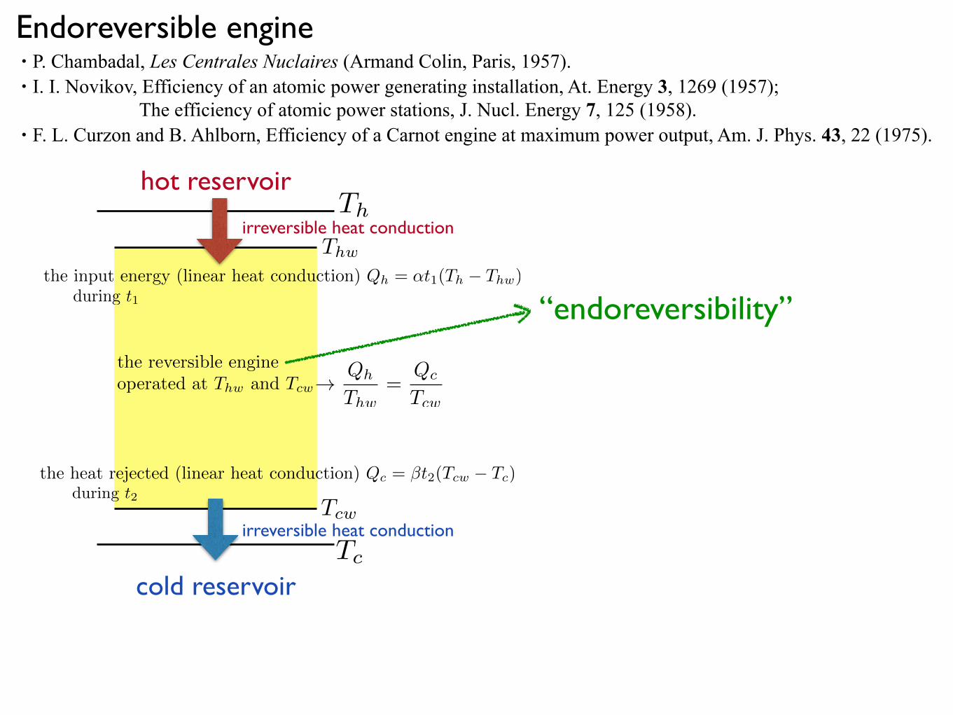
“endoreversibility”
Th
Tc
hot reservoir
cold reservoir
Thw
Tcw
during t1
irreversible heat conduction
the input energy (linear heat conduction) Qh = ↵t1(Th � Thw)
the reversible engine
operated at Thw and Tcw!Qh
Thw=
Qc
Tcw
during t2
irreversible heat conduction
the heat rejected (linear heat conduction) Qc = �t2(Tcw � Tc)
Endoreversible engine• P. Chambadal, Les Centrales Nuclaires (Armand Colin, Paris, 1957). • I. I. Novikov, Efficiency of an atomic power generating installation, At. Energy 3, 1269 (1957);
The efficiency of atomic power stations, J. Nucl. Energy 7, 125 (1958). • F. L. Curzon and B. Ahlborn, Efficiency of a Carnot engine at maximum power output, Am. J. Phys. 43, 22 (1975).
“endoreversibility”
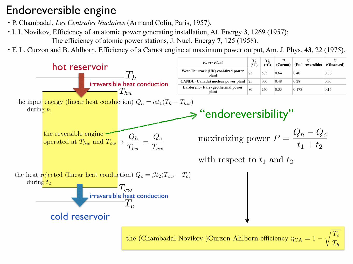
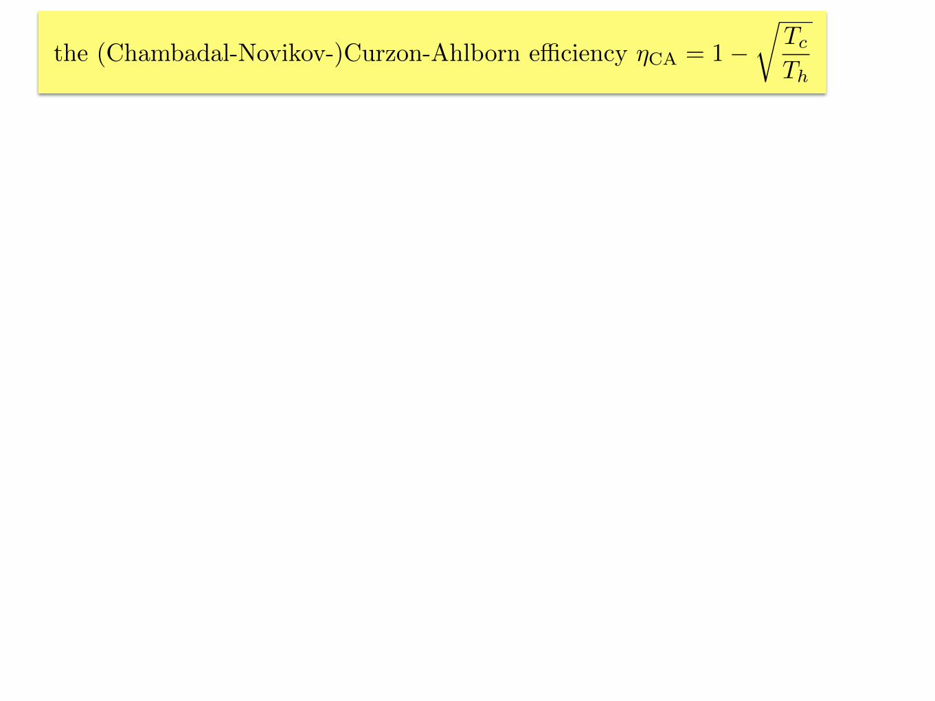
the (Chambadal-Novikov-)Curzon-Ahlborn e�ciency ⌘CA = 1�r
Tc
Th
Th
Tc
hot reservoir
cold reservoir
Thw
Tcw
during t1
irreversible heat conduction
the input energy (linear heat conduction) Qh = ↵t1(Th � Thw)
the reversible engine
operated at Thw and Tcw!Qh
Thw=
Qc
Tcw
during t2
irreversible heat conduction
the heat rejected (linear heat conduction) Qc = �t2(Tcw � Tc)
maximizing power P =
Qh �Qc
t1 + t2
with respect to t1 and t2
Endoreversible engine• P. Chambadal, Les Centrales Nuclaires (Armand Colin, Paris, 1957). • I. I. Novikov, Efficiency of an atomic power generating installation, At. Energy 3, 1269 (1957);
The efficiency of atomic power stations, J. Nucl. Energy 7, 125 (1958). • F. L. Curzon and B. Ahlborn, Efficiency of a Carnot engine at maximum power output, Am. J. Phys. 43, 22 (1975).3/31/16, 12:03Endoreversible thermodynamics - Wikipedia, the free encyclopedia
Page 2 of 3https://en.wikipedia.org/wiki/Endoreversible_thermodynamics
Power Plant (°C) (°C) (Carnot) (Endoreversible) (Observed)West Thurrock (UK) coal-fired power
plant 25 565 0.64 0.40 0.36
CANDU (Canada) nuclear power plant 25 300 0.48 0.28 0.30Larderello (Italy) geothermal power
plant 80 250 0.33 0.178 0.16
As shown, the endoreversible efficiency much more closely models the observed data. However, such anengine violates Carnot's principle which states that work can be done any time there is a difference intemperature. The fact that the hot and cold reservoirs are not at the same temperature as the working fluidthey are in contact with means that work can and is done at the hot and cold reservoirs. The result istantamount to coupling the high and low temperature parts of the cycle, so that the cycle collapses.[7] In theCarnot cycle there is strict necessity that the working fluid be at the same temperatures as the heat reservoirsthey are in contact with and that they are separated by adiabatic transformations which prevent thermalcontact. The efficiency was first derived by William Thomson [8] in his study of an unevenly heated body inwhich the adiabatic partitions between bodies at different temperatures are removed and maximum work isperformed. It is well known that the final temperature is the geometric mean temperature so that
the efficiency is the Carnot efficiency for an engine working between and .
Due to occasional confusion about the origins of the above equation, it is sometimes named theChambadal-Novikov-Curzon-Ahlborn efficiency.
See alsoHeat engine
An introduction to endoreversible thermodynamics is given in the thesis by Katharina Wagner.[4] It is alsointroduced by Hoffman et al.[9][10] A thorough discussion of the concept, together with many applications inengineering, is given in the book by Hans Ulrich Fuchs.[11]
References1. I. I. Novikov. The Efficiency of Atomic Power Stations. Journal Nuclear Energy II, 7:125–128, 1958. translated from
Atomnaya Energiya, 3 (1957), 409.2. Chambadal P (1957) Les centrales nucléaires. Armand Colin, Paris, France, 4 1-583. F.L. Curzon and B. Ahlborn, American Journal of Physics, vol. 43, pp. 22–24 (1975)4. M.Sc. Katharina Wagner, A graphic based interface to Endoreversible Thermodynamics, TU Chemnitz, Fakultät für
Naturwissenschaften, Masterarbeit (in English). http://archiv.tu-chemnitz.de/pub/2008/0123/index.html5. A Bejan, J. Appl. Phys., vol. 79, pp. 1191–1218, 1 Feb. 1996 http://dx.doi.org/10.1016/S0035-3159(96)80059-66. Callen, Herbert B. (1985). Thermodynamics and an Introduction to Thermostatistics (2nd ed. ed.). John Wiley &
Sons, Inc.. ISBN 0-471-86256-8.7. B. H. Lavenda, Am. J. Phys., vol. 75, pp. 169-175 (2007)8. W. Thomson, Phil. Mag. (Feb. 1853)
the (Chambadal-Novikov-)Curzon-Ahlborn e�ciency ⌘CA = 1�r
Tc
Th
the (Chambadal-Novikov-)Curzon-Ahlborn e�ciency ⌘CA = 1�r
Tc
Th
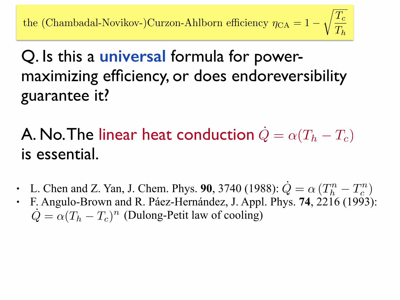
Q. Is this a universal formula for power-maximizing efficiency, or does endoreversibility guarantee it?
A. No. The linear heat conduction is essential.
Q̇ = ↵(Th � Tc)
• L. Chen and Z. Yan, J. Chem. Phys. 90, 3740 (1988): • F. Angulo-Brown and R. Páez-Hernández, J. Appl. Phys. 74, 2216 (1993):
(Dulong-Petit law of cooling)Q̇ = ↵(Th � Tc)n
Q̇ = ↵ (Tnh � Tn
c )
the (Chambadal-Novikov-)Curzon-Ahlborn e�ciency ⌘CA = 1�r
Tc
Th
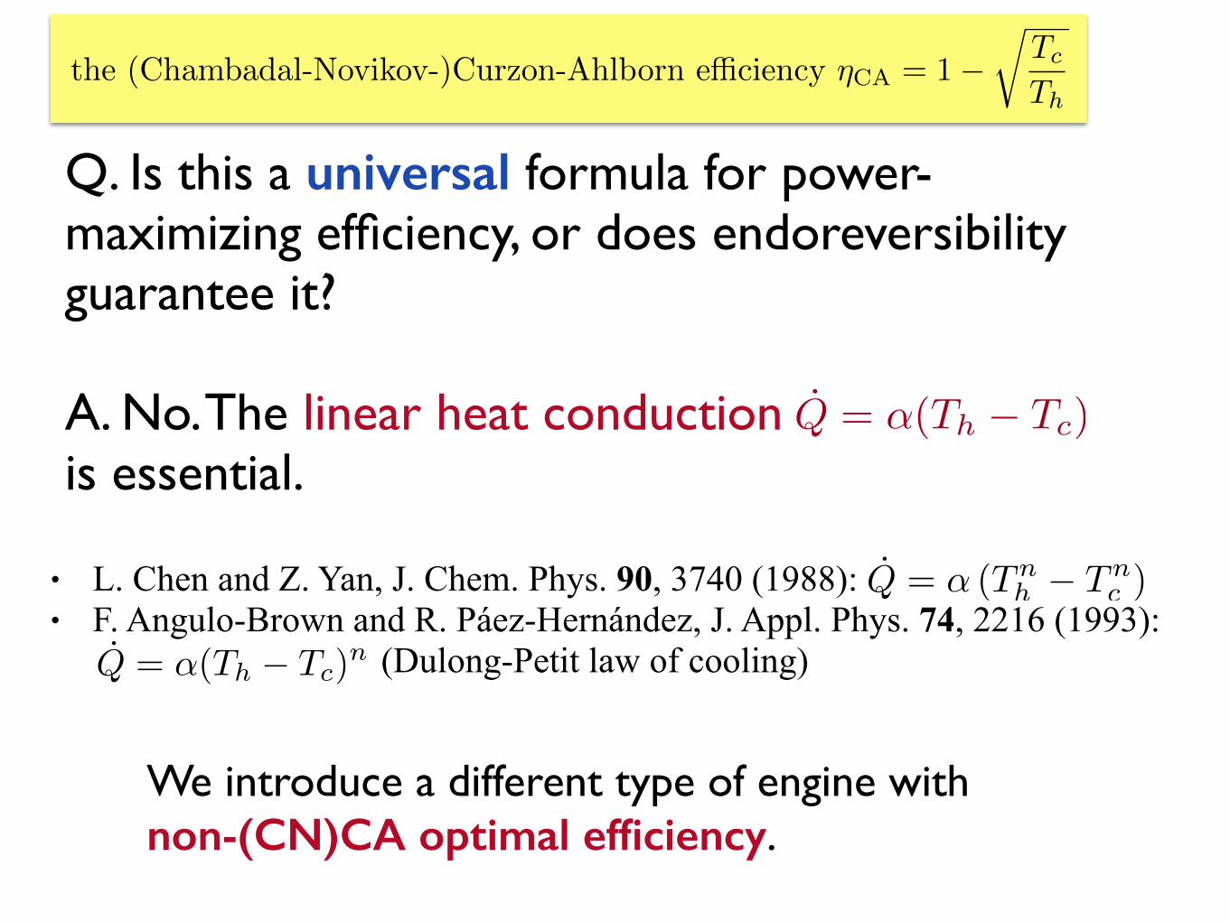
Q. Is this a universal formula for power-maximizing efficiency, or does endoreversibility guarantee it?
A. No. The linear heat conduction is essential.
Q̇ = ↵(Th � Tc)
We introduce a different type of engine with non-(CN)CA optimal efficiency.
• L. Chen and Z. Yan, J. Chem. Phys. 90, 3740 (1988): • F. Angulo-Brown and R. Páez-Hernández, J. Appl. Phys. 74, 2216 (1993):
(Dulong-Petit law of cooling)Q̇ = ↵(Th � Tc)n
Q̇ = ↵ (Tnh � Tn
c )
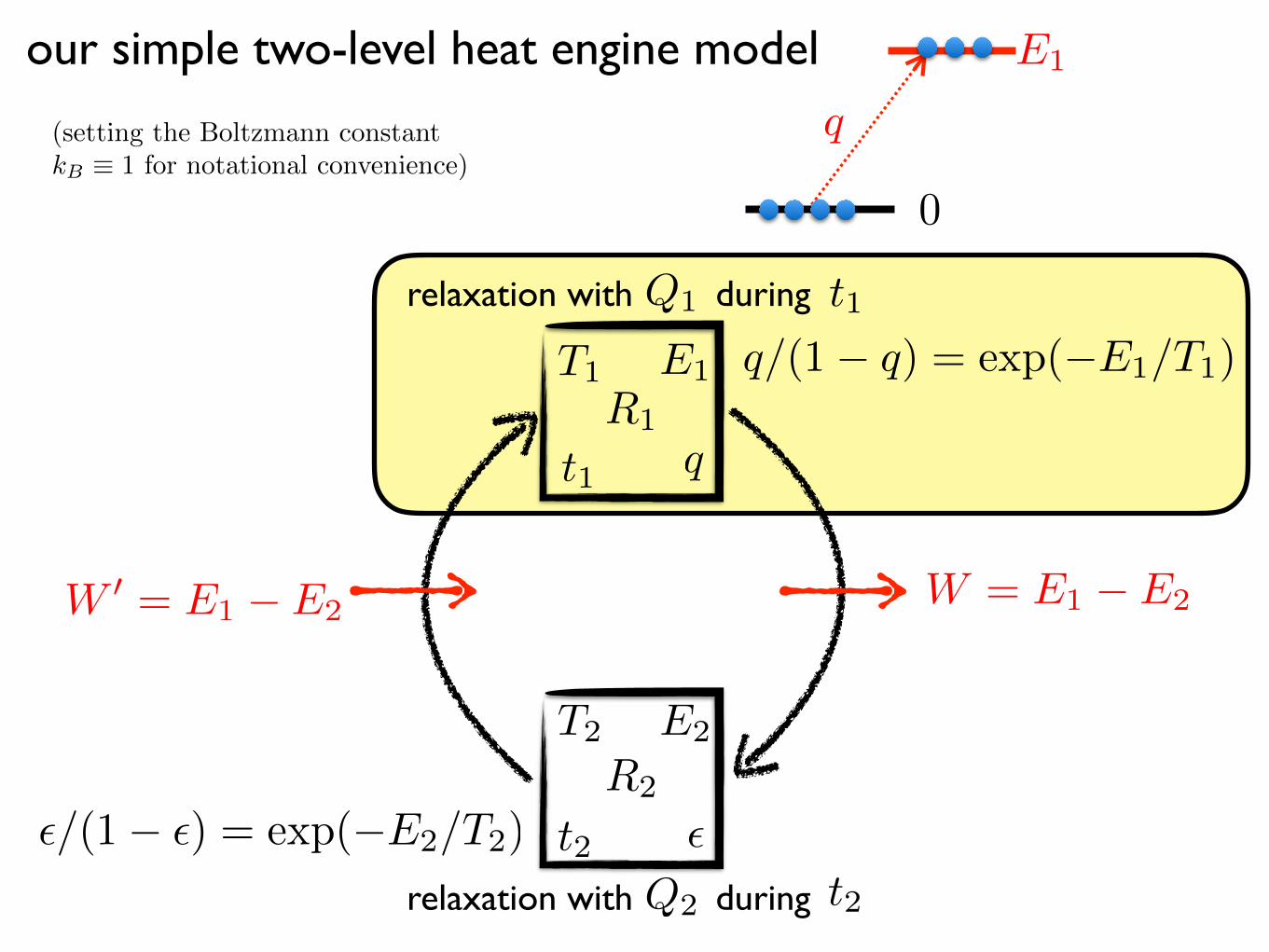
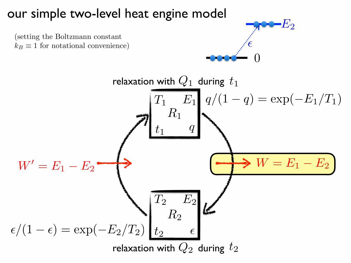
our simple two-level heat engine model
R1
R2
relaxation with
relaxation with
Q1
Q2
E1
E2
T1
T2
q
✏
t1
t2
during t1
during t2
W = E1 � E2W 0 = E1 � E2
q/(1� q) = exp(�E1/T1)
✏/(1� ✏) = exp(�E2/T2)
0
E1
q(setting the Boltzmann constant
kB ⌘ 1 for notational convenience)
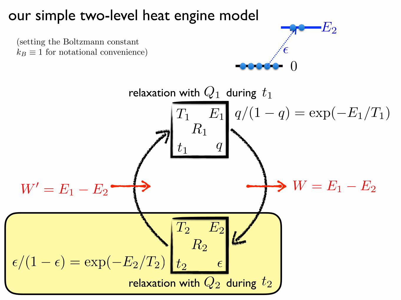
our simple two-level heat engine model
R1
R2
relaxation with
relaxation with
Q1
Q2
E1
E2
T1
T2
q
✏
t1
t2
during t1
during t2
W = E1 � E2W 0 = E1 � E2
q/(1� q) = exp(�E1/T1)
✏/(1� ✏) = exp(�E2/T2)
0
E2
✏(setting the Boltzmann constant
kB ⌘ 1 for notational convenience)
our simple two-level heat engine model
R1
R2
relaxation with
relaxation with
Q1
Q2
E1
E2
T1
T2
q
✏
t1
t2
during t1
during t2
W = E1 � E2W 0 = E1 � E2
q/(1� q) = exp(�E1/T1)
✏/(1� ✏) = exp(�E2/T2)
0
E2
✏(setting the Boltzmann constant
kB ⌘ 1 for notational convenience)
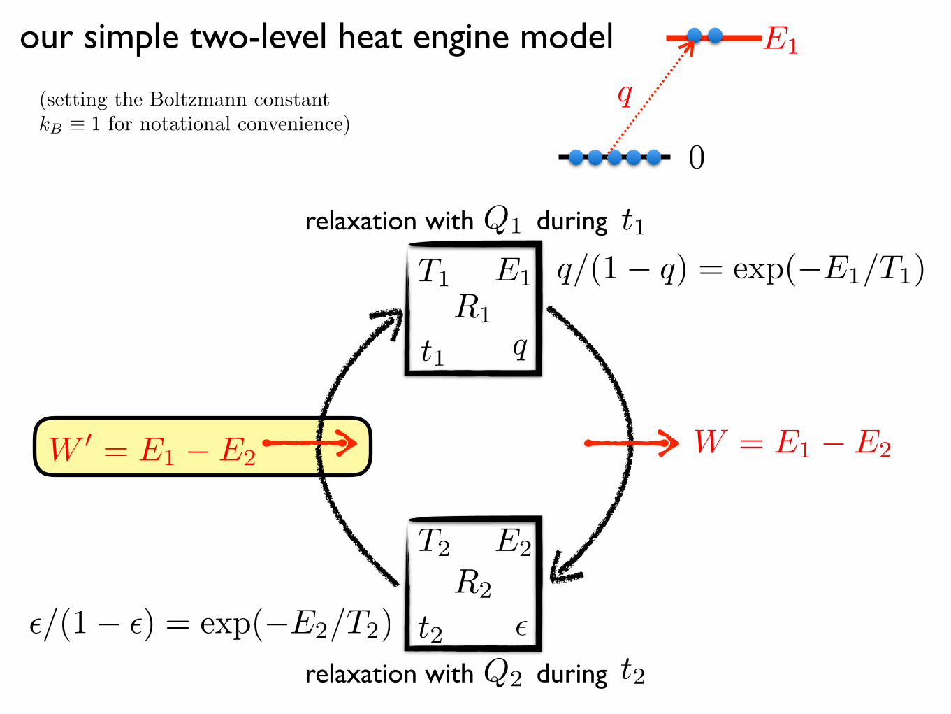
our simple two-level heat engine model
R1
R2
relaxation with
relaxation with
Q1
Q2
E1
E2
T1
T2
q
✏
t1
t2
during t1
during t2
W = E1 � E2W 0 = E1 � E2
q/(1� q) = exp(�E1/T1)
✏/(1� ✏) = exp(�E2/T2)
0
q
E1
(setting the Boltzmann constant
kB ⌘ 1 for notational convenience)

our simple two-level heat engine model
R1
R2
relaxation with
relaxation with
Q1
Q2
E1
E2
T1
T2
q
✏
t1
t2
during t1
during t2
W = E1 � E2W 0 = E1 � E2
q/(1� q) = exp(�E1/T1)
✏/(1� ✏) = exp(�E2/T2)
0
q
E1
(setting the Boltzmann constant
kB ⌘ 1 for notational convenience)
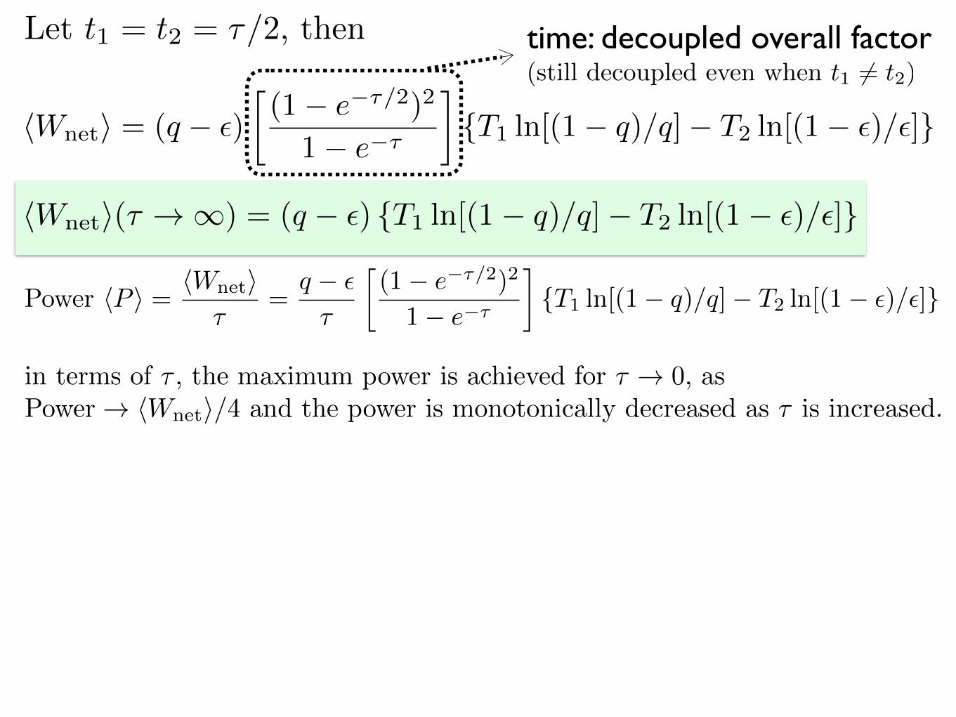
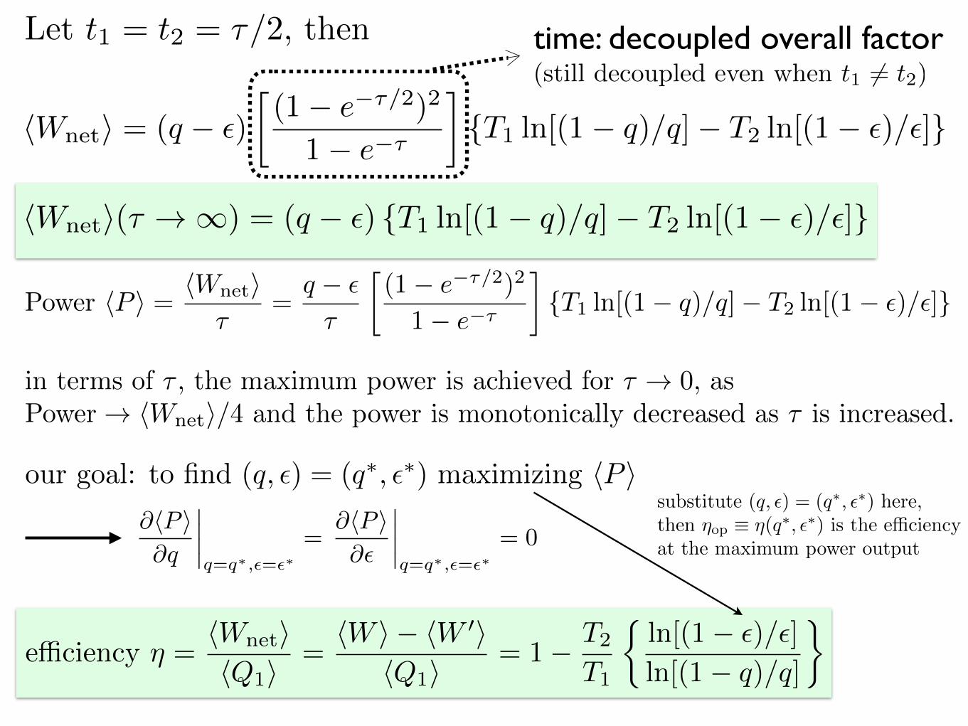
Let t1 = t2 = ⌧/2, then
in terms of ⌧ , the maximum power is achieved for ⌧ ! 0, as
Power ! hWneti/4 and the power is monotonically decreased as ⌧ is increased.
hWneti = (q � ✏)
(1� e�⌧/2)2
1� e�⌧
�{T1 ln[(1� q)/q]� T2 ln[(1� ✏)/✏]}
time: decoupled overall factor
hWneti(⌧ ! 1) = (q � ✏) {T1 ln[(1� q)/q]� T2 ln[(1� ✏)/✏]}
Power hP i = hWneti⌧
=
q � ✏
⌧
(1� e�⌧/2
)
2
1� e�⌧
�{T1 ln[(1� q)/q]� T2 ln[(1� ✏)/✏]}
(still decoupled even when t1 6= t2)
Let t1 = t2 = ⌧/2, then
in terms of ⌧ , the maximum power is achieved for ⌧ ! 0, as
Power ! hWneti/4 and the power is monotonically decreased as ⌧ is increased.
hWneti = (q � ✏)
(1� e�⌧/2)2
1� e�⌧
�{T1 ln[(1� q)/q]� T2 ln[(1� ✏)/✏]}
time: decoupled overall factor
hWneti(⌧ ! 1) = (q � ✏) {T1 ln[(1� q)/q]� T2 ln[(1� ✏)/✏]}
Power hP i = hWneti⌧
=
q � ✏
⌧
(1� e�⌧/2
)
2
1� e�⌧
�{T1 ln[(1� q)/q]� T2 ln[(1� ✏)/✏]}
our goal: to find (q, ✏) = (q⇤, ✏⇤) maximizing hP i@hP i@q
����q=q⇤,✏=✏⇤
=@hP i@✏
����q=q⇤,✏=✏⇤
= 0
(still decoupled even when t1 6= t2)
hWneti = hW i � hW 0i = (P1 � P2)(E1 � E2)= (P1 � P2){T1 ln[(1� q)/q]� T2 ln[(1� ✏)/✏]}
e�ciency ⌘ =hWnetihQ1i
=hW i � hW 0i
hQ1i= 1� T2
T1
⇢ln[(1� ✏)/✏]
ln[(1� q)/q]
�
substitute (q, ✏) = (q⇤, ✏⇤) here,then ⌘
op
⌘ ⌘(q⇤, ✏⇤) is the e�ciency
at the maximum power output
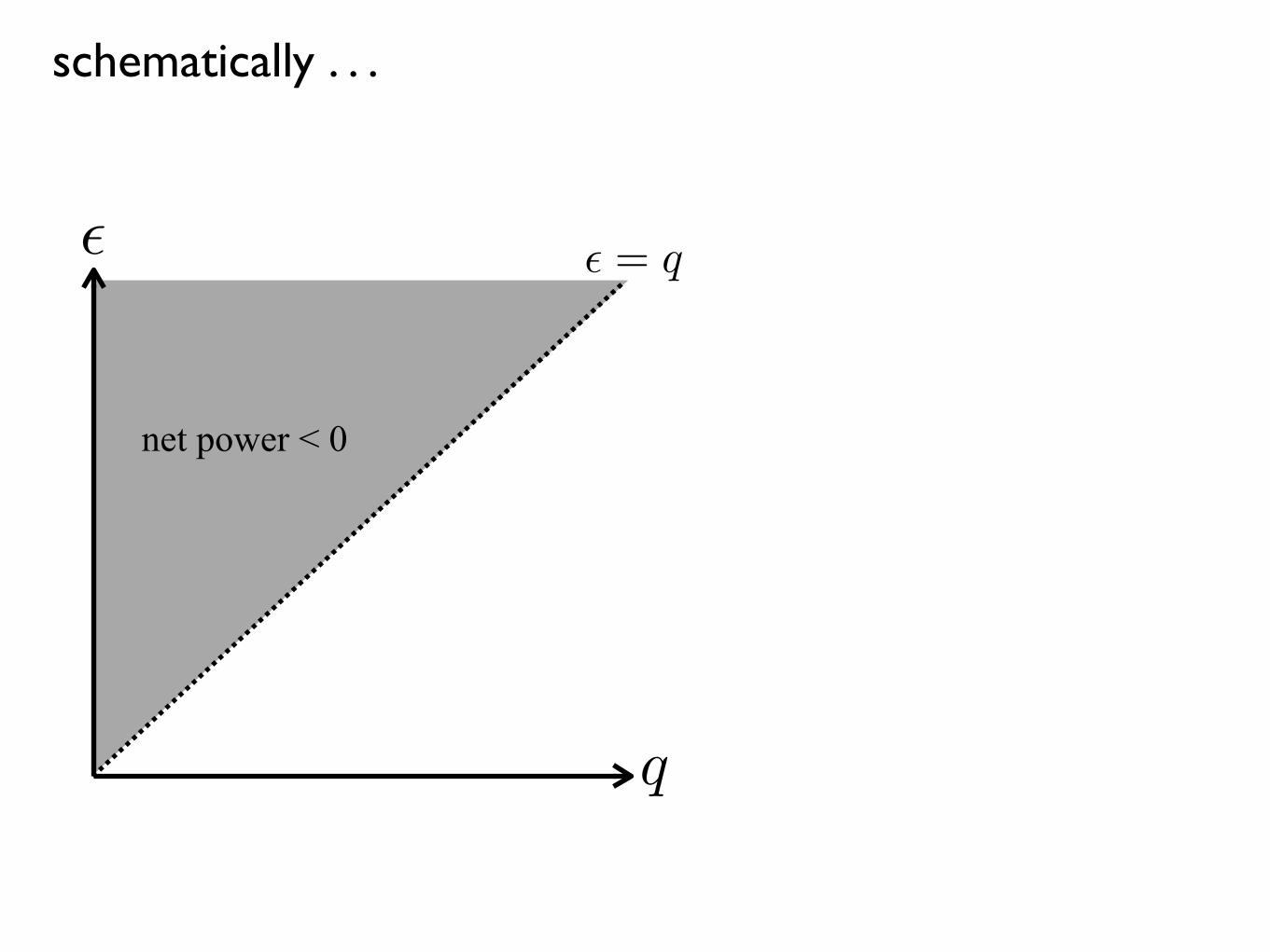
schematically . . .
✏
q
✏ = q
net power < 0
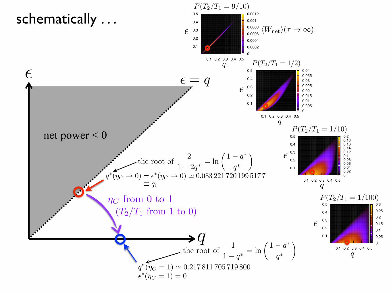
schematically . . .
✏
q
✏ = q
net power < 0
⌘C from 0 to 1
(T2/T1 from 1 to 0)
<Wnet>(τ → ∞), T1 = 1, T2 = 1/100
0.1 0.2 0.3 0.4 0.5q
0.1
0.2
0.3
0.4
0.5
ε
0
0.05
0.1
0.15
0.2
0.25
0.3
<Wnet>(τ → ∞), T1 = 1, T2 = 1/10
0.1 0.2 0.3 0.4 0.5q
0.1
0.2
0.3
0.4
0.5
ε
0 0.02 0.04 0.06 0.08 0.1 0.12 0.14 0.16 0.18 0.2
<Wnet>(τ → ∞), T1 = 1, T2 = 1/2
0.1 0.2 0.3 0.4 0.5q
0.1
0.2
0.3
0.4
0.5
ε
0 0.005 0.01 0.015 0.02 0.025 0.03 0.035 0.04
<Wnet>(τ → ∞), T1 = 1, T2 = 9/10
0.1 0.2 0.3 0.4 0.5q
0.1
0.2
0.3
0.4
0.5
ε
0
0.0002
0.0004
0.0006
0.0008
0.001
0.0012
P (T2/T1 = 9/10)
P (T2/T1 = 1/2)
P (T2/T1 = 1/10)
P (T2/T1 = 1/100)
q
q
q
✏
✏
✏
✏
q
hWneti(⌧ ! 1) = (q � ✏) {T1 ln[(1� q)/q]� T2 ln[(1� ✏)/✏]}
q⇤(⌘C ! 0) = ✏⇤(⌘C ! 0) ' 0.083 221 720 199 517 7⌘ q0
the root of
2
1� 2q⇤= ln
✓1� q⇤
q⇤
◆
q⇤(⌘C = 1) ' 0.217 811 705 719 800✏⇤(⌘C = 1) = 0
the root of
1
1� q⇤= ln
✓1� q⇤
q⇤
◆
4
0
0.05
0.1
0.15
0.2
0 0.2 0.4 0.6 0.8 1
q* a
nd ε
*
ηc = 1 − T2 / T1
q*ε*
q*(ηc→0) = ε*(ηc→0)q*(ηc=1)
ηc→1 asymptote
FIG. 3. Numerically found q
⇤ and ✏⇤ values satisfying Eq. (18), as afunction of ⌘
C
= 1�T2/T1, along with the q
⇤(⌘C
! 0) = ✏⇤(⌘C
! 0)and q
⇤(⌘C
= 1) values presented in Sec. III B 2. ✏⇤(⌘C
= 1) = 0 (thehorizontal axis). The ⌘
C
! 1 asymptote indicates Eq. (34).schematically . . .
�
q
� = q
no net work
as �C is increased
q�(�C � 0) = ��(�C � 0) � 0.083 221 720 199 517 7
q�(�C = 1) � 0.217 811 705 719 800��(�C = 1) = 0
FIG. 4. Illustration of the optimal transition rates (q⇤, ✏⇤) for the max-imum power output as the T2/T1 value varies.
2. Asymptotic behaviors obtained from series expansion
The upper bound for q
⇤ is given by the condition ⌘C
= 1,satisfying ln[(1 � q
⇤)/q⇤] = 1/(1 � q
⇤) and q
⇤(⌘C
= 1) '0.217 811 705 719 800 found numerically and ✏⇤(⌘
C
= 1) = 0exactly from Eq. (16b). ⌘
C
= 0 always satisfies Eq. (18) re-gardless of q
⇤ values, so finding the optimal q
⇤ is meaningless(in fact, when ⌘
C
= 0, the operating regime for the engineis shrunk to the line q = ✏ and there cannot be any positivework). Therefore, let us examine the case ⌘
C
' 0 using theseries expansion of q
⇤ with respect to ⌘C
, as
q
⇤ = q0 + a1⌘C
+ a2⌘2C
+ a3⌘3C
+ O⇣⌘4
C
⌘. (22)
Substituting Eq. (22) into Eq. (18) and expanding the left-handside with respect to ⌘
C
again, we obtain
2 � (1 � 2q0) ln[(1 � q0)/q0]2q0 � 1
⌘C
+q0(1 � q0) � 2a1(1 � 2q0)
2(1 � q0)q0(1 � 2q0)3 ⌘2C
+ c3(q0, a1, a2)⌘3C
+ O⇣⌘4
C
⌘= 0 ,
(23)
where c3(q0, a1, a2) = [10q
60 + 3a
21 � 6q0(a2
1 + a2) � 6q
50(5 +
6a1+8a2)�12q
30(1+6a1+16a
21+9a2)+q
20(1+18a1+132a
21+
42a2)+q
40(31+90a1+96a
21+120a2)]/[6(1�2q0)5(1�q0)2
q
20].
Letting the linear coe�cient to be zero yields
21 � 2q0
= ln
1 � q0
q0
!, (24)
from which the lower bound for q
⇤(⌘C
! 0) = q0 =✏⇤(⌘
C
! 0) ' 0.083 221 720 199 517 7 found numerically[lim⌘
C
!0 U(⌘C
, q⇤) = 1 � 2q
⇤, thus ✏⇤(⌘C
! 0) = q
⇤(⌘C
! 0)by Eq. (16b)]. Figure 3 shows the numerical solution (q⇤, ✏⇤)as a function of ⌘
C
, where the asymptotic behaviors derivedabove hold when ⌘
C
' 0 and ⌘C
' 1. It seems that q
⇤ ismonotonically increased and ✏⇤ is monotonically decreased,as ⌘
C
is increased, i.e., q
⇤min = q
⇤(⌘C
! 0), q
⇤max = q
⇤(⌘C
= 1),✏⇤min = 0, and ✏⇤max = ✏
⇤(⌘C
! 0). Figure 4 illustrates the situ-ation on the (q, ✏) plane. The linear coe�cient a1 in Eq. (22)can be written in terms of q0 when we let the coe�cient of thequadratic term in Eq. (23) to be zero, as
a1 =q0(1 � q0)2(1 � 2q0)
. (25)
Similarly, the coe�cient a2 in Eq. (22) can also be written interms of q0 alone, by letting c3(q0, a1, a2) = 0 in Eq. (23) andusing the relations in Eqs. (24) and (25), as
a2 =7q0(1 � q0)24(1 � 2q0)
. (26)
With the relations of coe�cients in hand, we find theasymptotic behavior of ⌘op in Eq. (19) by expanding it withrespect to ⌘
C
after substituting q
⇤ as the series expansion of⌘
C
in Eq. (22). Then,
⌘op =1
(1 � 2q0) ln[(1 � q0)/q0]⌘
C
+
a1q0�3q
20+2q
30+
[q20+2a1�q0(1+4a1)] ln[(1�q0)/q0]
(1�2q0)3
ln2[(1 � q0)/q0]⌘2
C
+ d3(q0, a1, a2)⌘3C
+ O⇣⌘4
C
⌘,
(27)
where d3(q0, a1, a2) = {2(1 � 2q0)2a1[q2
0 + 2a1 � q0(1 +4a1)] ln[(1�q0)/q0]+2[�2q
40+a1�4a
21�2a2+4q0(4a
21+3a2)+
4q
30(1+a1+4a2)�2q
20(1+3a1+8a
21+12a2)] ln2[(1�q0)/q0]+(1�
2q0)4{�2a
21+[(1�2q0)a2
1�2(1�q0)q0a2] ln[(1�q0)/q0]}}/[(1�q
20)2
q
20]. Using Eqs. (24), (25) and (26), Eq. (27) becomes sim-
ply
⌘op =12⌘
C
+18⌘2
C
+7 � 24q0 + 24q
20
96(1 � 2q0)2 ⌘3C
+ O⇣⌘4
C
⌘. (28)
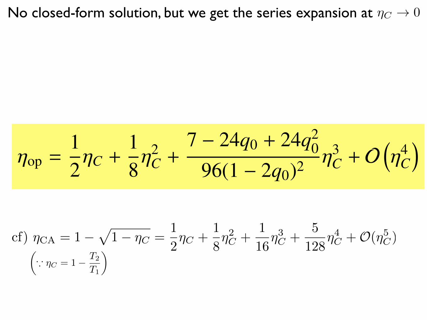
No closed-form solution, but we get the series expansion at
cf) ⌘CA = 1�p
1� ⌘C =1
2⌘C +
1
8⌘2C +
1
16⌘3C +
5
128⌘4C +O(⌘5C)
✓* ⌘C = 1� T2
T1
◆
⌘C ! 0
4
0
0.05
0.1
0.15
0.2
0 0.2 0.4 0.6 0.8 1
q* a
nd ε
*
ηc = 1 − T2 / T1
q*ε*
q*(ηc→0) = ε*(ηc→0)q*(ηc=1)
ηc→1 asymptote
FIG. 3. Numerically found q
⇤ and ✏⇤ values satisfying Eq. (18), as afunction of ⌘
C
= 1�T2/T1, along with the q
⇤(⌘C
! 0) = ✏⇤(⌘C
! 0)and q
⇤(⌘C
= 1) values presented in Sec. III B 2. ✏⇤(⌘C
= 1) = 0 (thehorizontal axis). The ⌘
C
! 1 asymptote indicates Eq. (34).schematically . . .
�
q
� = q
no net work
as �C is increased
q�(�C � 0) = ��(�C � 0) � 0.083 221 720 199 517 7
q�(�C = 1) � 0.217 811 705 719 800��(�C = 1) = 0
FIG. 4. Illustration of the optimal transition rates (q⇤, ✏⇤) for the max-imum power output as the T2/T1 value varies.
2. Asymptotic behaviors obtained from series expansion
The upper bound for q
⇤ is given by the condition ⌘C
= 1,satisfying ln[(1 � q
⇤)/q⇤] = 1/(1 � q
⇤) and q
⇤(⌘C
= 1) '0.217 811 705 719 800 found numerically and ✏⇤(⌘
C
= 1) = 0exactly from Eq. (16b). ⌘
C
= 0 always satisfies Eq. (18) re-gardless of q
⇤ values, so finding the optimal q
⇤ is meaningless(in fact, when ⌘
C
= 0, the operating regime for the engineis shrunk to the line q = ✏ and there cannot be any positivework). Therefore, let us examine the case ⌘
C
' 0 using theseries expansion of q
⇤ with respect to ⌘C
, as
q
⇤ = q0 + a1⌘C
+ a2⌘2C
+ a3⌘3C
+ O⇣⌘4
C
⌘. (22)
Substituting Eq. (22) into Eq. (18) and expanding the left-handside with respect to ⌘
C
again, we obtain
2 � (1 � 2q0) ln[(1 � q0)/q0]2q0 � 1
⌘C
+q0(1 � q0) � 2a1(1 � 2q0)
2(1 � q0)q0(1 � 2q0)3 ⌘2C
+ c3(q0, a1, a2)⌘3C
+ O⇣⌘4
C
⌘= 0 ,
(23)
where c3(q0, a1, a2) = [10q
60 + 3a
21 � 6q0(a2
1 + a2) � 6q
50(5 +
6a1+8a2)�12q
30(1+6a1+16a
21+9a2)+q
20(1+18a1+132a
21+
42a2)+q
40(31+90a1+96a
21+120a2)]/[6(1�2q0)5(1�q0)2
q
20].
Letting the linear coe�cient to be zero yields
21 � 2q0
= ln
1 � q0
q0
!, (24)
from which the lower bound for q
⇤(⌘C
! 0) = q0 =✏⇤(⌘
C
! 0) ' 0.083 221 720 199 517 7 found numerically[lim⌘
C
!0 U(⌘C
, q⇤) = 1 � 2q
⇤, thus ✏⇤(⌘C
! 0) = q
⇤(⌘C
! 0)by Eq. (16b)]. Figure 3 shows the numerical solution (q⇤, ✏⇤)as a function of ⌘
C
, where the asymptotic behaviors derivedabove hold when ⌘
C
' 0 and ⌘C
' 1. It seems that q
⇤ ismonotonically increased and ✏⇤ is monotonically decreased,as ⌘
C
is increased, i.e., q
⇤min = q
⇤(⌘C
! 0), q
⇤max = q
⇤(⌘C
= 1),✏⇤min = 0, and ✏⇤max = ✏
⇤(⌘C
! 0). Figure 4 illustrates the situ-ation on the (q, ✏) plane. The linear coe�cient a1 in Eq. (22)can be written in terms of q0 when we let the coe�cient of thequadratic term in Eq. (23) to be zero, as
a1 =q0(1 � q0)2(1 � 2q0)
. (25)
Similarly, the coe�cient a2 in Eq. (22) can also be written interms of q0 alone, by letting c3(q0, a1, a2) = 0 in Eq. (23) andusing the relations in Eqs. (24) and (25), as
a2 =7q0(1 � q0)24(1 � 2q0)
. (26)
With the relations of coe�cients in hand, we find theasymptotic behavior of ⌘op in Eq. (19) by expanding it withrespect to ⌘
C
after substituting q
⇤ as the series expansion of⌘
C
in Eq. (22). Then,
⌘op =1
(1 � 2q0) ln[(1 � q0)/q0]⌘
C
+
a1q0�3q
20+2q
30+
[q20+2a1�q0(1+4a1)] ln[(1�q0)/q0]
(1�2q0)3
ln2[(1 � q0)/q0]⌘2
C
+ d3(q0, a1, a2)⌘3C
+ O⇣⌘4
C
⌘,
(27)
where d3(q0, a1, a2) = {2(1 � 2q0)2a1[q2
0 + 2a1 � q0(1 +4a1)] ln[(1�q0)/q0]+2[�2q
40+a1�4a
21�2a2+4q0(4a
21+3a2)+
4q
30(1+a1+4a2)�2q
20(1+3a1+8a
21+12a2)] ln2[(1�q0)/q0]+(1�
2q0)4{�2a
21+[(1�2q0)a2
1�2(1�q0)q0a2] ln[(1�q0)/q0]}}/[(1�q
20)2
q
20]. Using Eqs. (24), (25) and (26), Eq. (27) becomes sim-
ply
⌘op =12⌘
C
+18⌘2
C
+7 � 24q0 + 24q
20
96(1 � 2q0)2 ⌘3C
+ O⇣⌘4
C
⌘. (28)
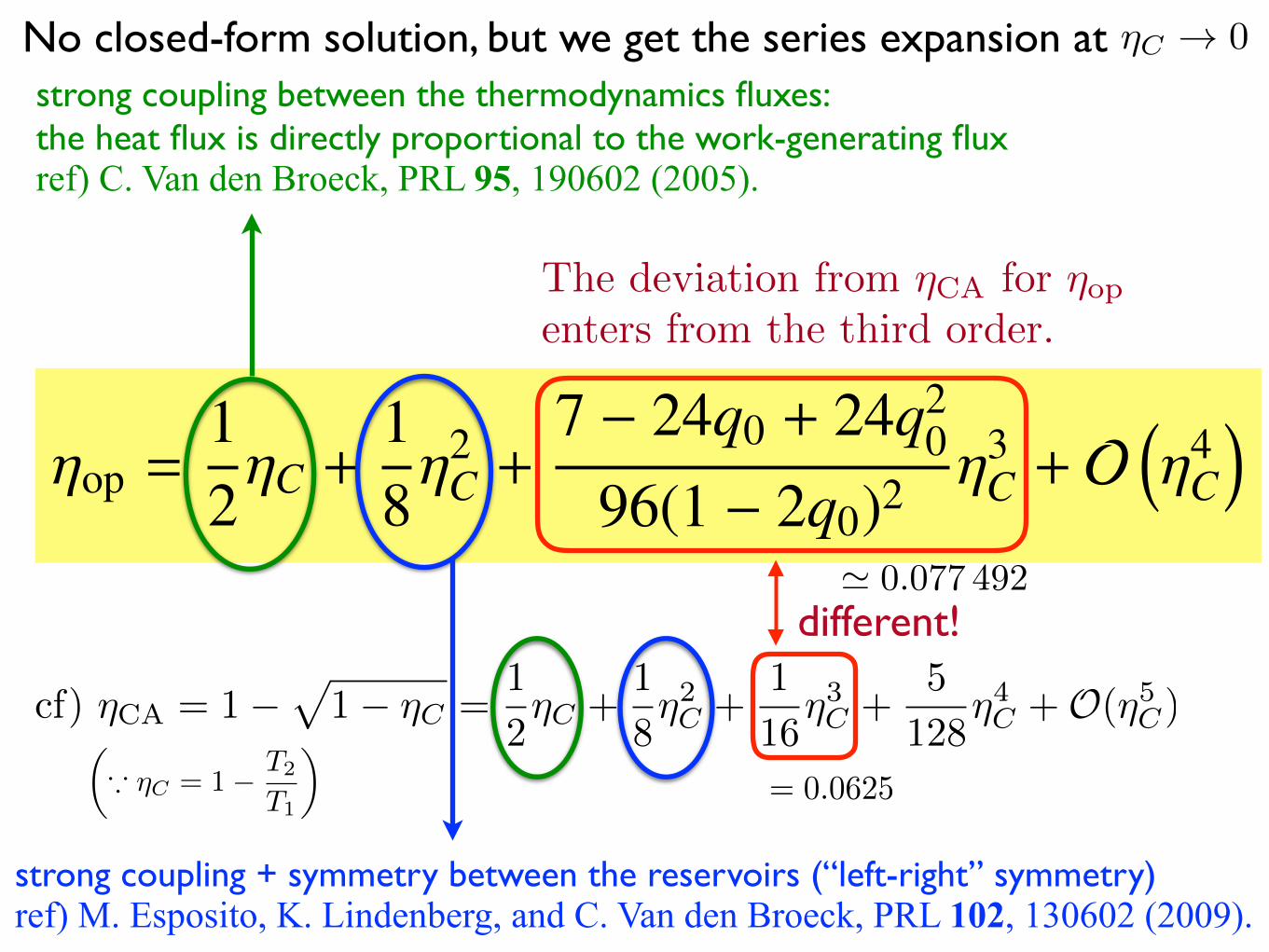
different!' 0.077 492
= 0.0625
strong coupling between the thermodynamics fluxes: the heat flux is directly proportional to the work-generating flux ref) C. Van den Broeck, PRL 95, 190602 (2005).
strong coupling + symmetry between the reservoirs (“left-right” symmetry) ref) M. Esposito, K. Lindenberg, and C. Van den Broeck, PRL 102, 130602 (2009).
The deviation from ⌘CA
for ⌘op
enters from the third order.
No closed-form solution, but we get the series expansion at
cf) ⌘CA = 1�p
1� ⌘C =1
2⌘C +
1
8⌘2C +
1
16⌘3C +
5
128⌘4C +O(⌘5C)
✓* ⌘C = 1� T2
T1
◆
⌘C ! 0
0
0.2
0.4
0.6
0.8
1
0 0.2 0.4 0.6 0.8 1
ηop
ηc
at (q*, ε*)ηCA = 1−√1−ηc
ηc/(2−ηc)ηc/2
ηc→1 asymptote
0.88
0.92
0.96
1
0.97 0.98 0.99 1
ηop
ηc
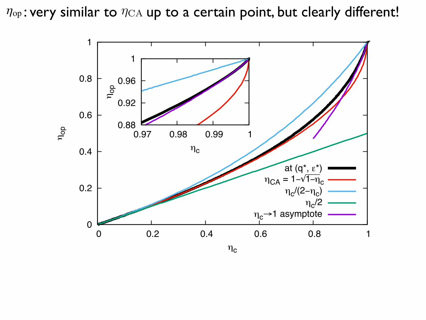
: very similar to up to a certain point, but clearly different!
4
0
0.05
0.1
0.15
0.2
0 0.2 0.4 0.6 0.8 1
q* a
nd ε*
ηc = 1 − T2 / T1
q*ε*
q*(ηc→0) = ε*(ηc→0)q*(ηc=1)
ηc→1 asymptote
FIG. 3. Numerically found q
⇤ and ✏⇤ values satisfying Eq. (18), as afunction of ⌘
C
= 1�T2/T1, along with the q
⇤(⌘C
! 0) = ✏⇤(⌘C
! 0)and q
⇤(⌘C
= 1) values presented in Sec. III B 2. ✏⇤(⌘C
= 1) = 0 (thehorizontal axis). The ⌘
C
! 1 asymptote indicates Eq. (34).schematically . . .
�
q
� = q
no net work
as �C is increased
q�(�C � 0) = ��(�C � 0) � 0.083 221 720 199 517 7
q�(�C = 1) � 0.217 811 705 719 800��(�C = 1) = 0
FIG. 4. Illustration of the optimal transition rates (q⇤, ✏⇤) for the max-imum power output as the T2/T1 value varies.
2. Asymptotic behaviors obtained from series expansion
The upper bound for q
⇤ is given by the condition ⌘C
= 1,satisfying ln[(1 � q
⇤)/q⇤] = 1/(1 � q
⇤) and q
⇤(⌘C
= 1) '0.217 811 705 719 800 found numerically and ✏⇤(⌘
C
= 1) = 0exactly from Eq. (16b). ⌘
C
= 0 always satisfies Eq. (18) re-gardless of q
⇤ values, so finding the optimal q
⇤ is meaningless(in fact, when ⌘
C
= 0, the operating regime for the engineis shrunk to the line q = ✏ and there cannot be any positivework). Therefore, let us examine the case ⌘
C
' 0 using theseries expansion of q
⇤ with respect to ⌘C
, as
q
⇤ = q0 + a1⌘C
+ a2⌘2C
+ a3⌘3C
+ O⇣⌘4
C
⌘. (22)
Substituting Eq. (22) into Eq. (18) and expanding the left-handside with respect to ⌘
C
again, we obtain
2 � (1 � 2q0) ln[(1 � q0)/q0]2q0 � 1
⌘C
+q0(1 � q0) � 2a1(1 � 2q0)
2(1 � q0)q0(1 � 2q0)3 ⌘2C
+ c3(q0, a1, a2)⌘3C
+ O⇣⌘4
C
⌘= 0 ,
(23)
where c3(q0, a1, a2) = [10q
60 + 3a
21 � 6q0(a2
1 + a2) � 6q
50(5 +
6a1+8a2)�12q
30(1+6a1+16a
21+9a2)+q
20(1+18a1+132a
21+
42a2)+q
40(31+90a1+96a
21+120a2)]/[6(1�2q0)5(1�q0)2
q
20].
Letting the linear coe�cient to be zero yields
21 � 2q0
= ln
1 � q0
q0
!, (24)
from which the lower bound for q
⇤(⌘C
! 0) = q0 =✏⇤(⌘
C
! 0) ' 0.083 221 720 199 517 7 found numerically[lim⌘
C
!0 U(⌘C
, q⇤) = 1 � 2q
⇤, thus ✏⇤(⌘C
! 0) = q
⇤(⌘C
! 0)by Eq. (16b)]. Figure 3 shows the numerical solution (q⇤, ✏⇤)as a function of ⌘
C
, where the asymptotic behaviors derivedabove hold when ⌘
C
' 0 and ⌘C
' 1. It seems that q
⇤ ismonotonically increased and ✏⇤ is monotonically decreased,as ⌘
C
is increased, i.e., q
⇤min = q
⇤(⌘C
! 0), q
⇤max = q
⇤(⌘C
= 1),✏⇤min = 0, and ✏⇤max = ✏
⇤(⌘C
! 0). Figure 4 illustrates the situ-ation on the (q, ✏) plane. The linear coe�cient a1 in Eq. (22)can be written in terms of q0 when we let the coe�cient of thequadratic term in Eq. (23) to be zero, as
a1 =q0(1 � q0)2(1 � 2q0)
. (25)
Similarly, the coe�cient a2 in Eq. (22) can also be written interms of q0 alone, by letting c3(q0, a1, a2) = 0 in Eq. (23) andusing the relations in Eqs. (24) and (25), as
a2 =7q0(1 � q0)24(1 � 2q0)
. (26)
With the relations of coe�cients in hand, we find theasymptotic behavior of ⌘op in Eq. (19) by expanding it withrespect to ⌘
C
after substituting q
⇤ as the series expansion of⌘
C
in Eq. (22). Then,
⌘op =1
(1 � 2q0) ln[(1 � q0)/q0]⌘
C
+
a1q0�3q
20+2q
30+
[q20+2a1�q0(1+4a1)] ln[(1�q0)/q0]
(1�2q0)3
ln2[(1 � q0)/q0]⌘2
C
+ d3(q0, a1, a2)⌘3C
+ O⇣⌘4
C
⌘,
(27)
where d3(q0, a1, a2) = {2(1 � 2q0)2a1[q2
0 + 2a1 � q0(1 +4a1)] ln[(1�q0)/q0]+2[�2q
40+a1�4a
21�2a2+4q0(4a
21+3a2)+
4q
30(1+a1+4a2)�2q
20(1+3a1+8a
21+12a2)] ln2[(1�q0)/q0]+(1�
2q0)4{�2a
21+[(1�2q0)a2
1�2(1�q0)q0a2] ln[(1�q0)/q0]}}/[(1�q
20)2
q
20]. Using Eqs. (24), (25) and (26), Eq. (27) becomes sim-
ply
⌘op =12⌘
C
+18⌘2
C
+7 � 24q0 + 24q
20
96(1 � 2q0)2 ⌘3C
+ O⇣⌘4
C
⌘. (28)cf) ⌘CA = 1�
p1� ⌘C =
1
2⌘C +
1
8⌘2C +
1
16⌘3C +
5
128⌘4C +O(⌘5C)
0
0.2
0.4
0.6
0.8
1
0 0.2 0.4 0.6 0.8 1
ηop
ηc
at (q*, ε*)ηCA = 1−√1−ηc
ηc/(2−ηc)ηc/2
ηc→1 asymptote
0.88
0.92
0.96
1
0.97 0.98 0.99 1
ηop
ηc
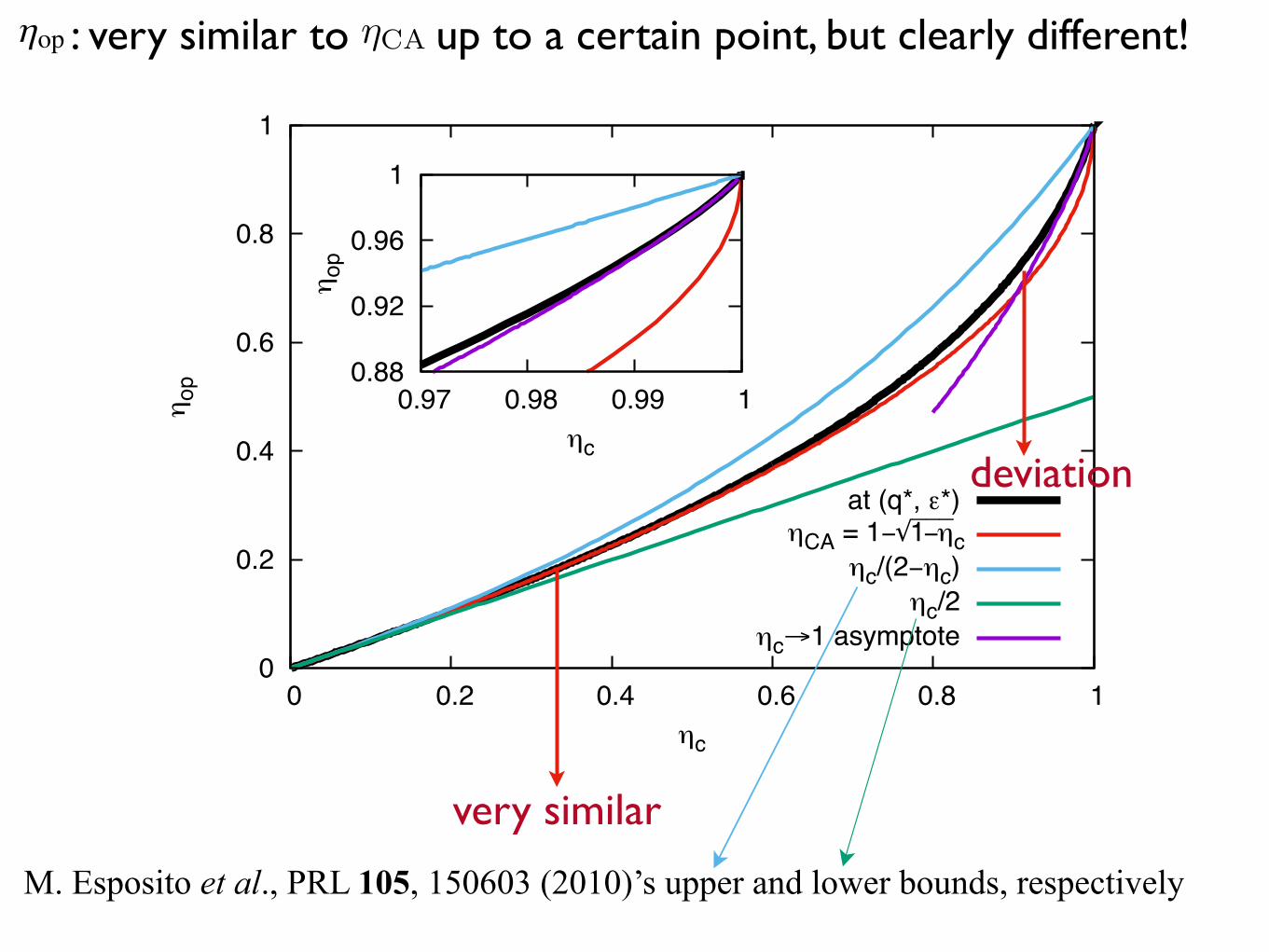
M. Esposito et al., PRL 105, 150603 (2010)’s upper and lower bounds, respectively
deviation
very similar
: very similar to up to a certain point, but clearly different!
4
0
0.05
0.1
0.15
0.2
0 0.2 0.4 0.6 0.8 1
q* a
nd ε*
ηc = 1 − T2 / T1
q*ε*
q*(ηc→0) = ε*(ηc→0)q*(ηc=1)
ηc→1 asymptote
FIG. 3. Numerically found q
⇤ and ✏⇤ values satisfying Eq. (18), as afunction of ⌘
C
= 1�T2/T1, along with the q
⇤(⌘C
! 0) = ✏⇤(⌘C
! 0)and q
⇤(⌘C
= 1) values presented in Sec. III B 2. ✏⇤(⌘C
= 1) = 0 (thehorizontal axis). The ⌘
C
! 1 asymptote indicates Eq. (34).schematically . . .
�
q
� = q
no net work
as �C is increased
q�(�C � 0) = ��(�C � 0) � 0.083 221 720 199 517 7
q�(�C = 1) � 0.217 811 705 719 800��(�C = 1) = 0
FIG. 4. Illustration of the optimal transition rates (q⇤, ✏⇤) for the max-imum power output as the T2/T1 value varies.
2. Asymptotic behaviors obtained from series expansion
The upper bound for q
⇤ is given by the condition ⌘C
= 1,satisfying ln[(1 � q
⇤)/q⇤] = 1/(1 � q
⇤) and q
⇤(⌘C
= 1) '0.217 811 705 719 800 found numerically and ✏⇤(⌘
C
= 1) = 0exactly from Eq. (16b). ⌘
C
= 0 always satisfies Eq. (18) re-gardless of q
⇤ values, so finding the optimal q
⇤ is meaningless(in fact, when ⌘
C
= 0, the operating regime for the engineis shrunk to the line q = ✏ and there cannot be any positivework). Therefore, let us examine the case ⌘
C
' 0 using theseries expansion of q
⇤ with respect to ⌘C
, as
q
⇤ = q0 + a1⌘C
+ a2⌘2C
+ a3⌘3C
+ O⇣⌘4
C
⌘. (22)
Substituting Eq. (22) into Eq. (18) and expanding the left-handside with respect to ⌘
C
again, we obtain
2 � (1 � 2q0) ln[(1 � q0)/q0]2q0 � 1
⌘C
+q0(1 � q0) � 2a1(1 � 2q0)
2(1 � q0)q0(1 � 2q0)3 ⌘2C
+ c3(q0, a1, a2)⌘3C
+ O⇣⌘4
C
⌘= 0 ,
(23)
where c3(q0, a1, a2) = [10q
60 + 3a
21 � 6q0(a2
1 + a2) � 6q
50(5 +
6a1+8a2)�12q
30(1+6a1+16a
21+9a2)+q
20(1+18a1+132a
21+
42a2)+q
40(31+90a1+96a
21+120a2)]/[6(1�2q0)5(1�q0)2
q
20].
Letting the linear coe�cient to be zero yields
21 � 2q0
= ln
1 � q0
q0
!, (24)
from which the lower bound for q
⇤(⌘C
! 0) = q0 =✏⇤(⌘
C
! 0) ' 0.083 221 720 199 517 7 found numerically[lim⌘
C
!0 U(⌘C
, q⇤) = 1 � 2q
⇤, thus ✏⇤(⌘C
! 0) = q
⇤(⌘C
! 0)by Eq. (16b)]. Figure 3 shows the numerical solution (q⇤, ✏⇤)as a function of ⌘
C
, where the asymptotic behaviors derivedabove hold when ⌘
C
' 0 and ⌘C
' 1. It seems that q
⇤ ismonotonically increased and ✏⇤ is monotonically decreased,as ⌘
C
is increased, i.e., q
⇤min = q
⇤(⌘C
! 0), q
⇤max = q
⇤(⌘C
= 1),✏⇤min = 0, and ✏⇤max = ✏
⇤(⌘C
! 0). Figure 4 illustrates the situ-ation on the (q, ✏) plane. The linear coe�cient a1 in Eq. (22)can be written in terms of q0 when we let the coe�cient of thequadratic term in Eq. (23) to be zero, as
a1 =q0(1 � q0)2(1 � 2q0)
. (25)
Similarly, the coe�cient a2 in Eq. (22) can also be written interms of q0 alone, by letting c3(q0, a1, a2) = 0 in Eq. (23) andusing the relations in Eqs. (24) and (25), as
a2 =7q0(1 � q0)24(1 � 2q0)
. (26)
With the relations of coe�cients in hand, we find theasymptotic behavior of ⌘op in Eq. (19) by expanding it withrespect to ⌘
C
after substituting q
⇤ as the series expansion of⌘
C
in Eq. (22). Then,
⌘op =1
(1 � 2q0) ln[(1 � q0)/q0]⌘
C
+
a1q0�3q
20+2q
30+
[q20+2a1�q0(1+4a1)] ln[(1�q0)/q0]
(1�2q0)3
ln2[(1 � q0)/q0]⌘2
C
+ d3(q0, a1, a2)⌘3C
+ O⇣⌘4
C
⌘,
(27)
where d3(q0, a1, a2) = {2(1 � 2q0)2a1[q2
0 + 2a1 � q0(1 +4a1)] ln[(1�q0)/q0]+2[�2q
40+a1�4a
21�2a2+4q0(4a
21+3a2)+
4q
30(1+a1+4a2)�2q
20(1+3a1+8a
21+12a2)] ln2[(1�q0)/q0]+(1�
2q0)4{�2a
21+[(1�2q0)a2
1�2(1�q0)q0a2] ln[(1�q0)/q0]}}/[(1�q
20)2
q
20]. Using Eqs. (24), (25) and (26), Eq. (27) becomes sim-
ply
⌘op =12⌘
C
+18⌘2
C
+7 � 24q0 + 24q
20
96(1 � 2q0)2 ⌘3C
+ O⇣⌘4
C
⌘. (28)cf) ⌘CA = 1�
p1� ⌘C =
1
2⌘C +
1
8⌘2C +
1
16⌘3C +
5
128⌘4C +O(⌘5C)
0
0.2
0.4
0.6
0.8
1
0 0.2 0.4 0.6 0.8 1
ηop
ηc
at (q*, ε*)ηCA = 1−√1−ηc
ηc/(2−ηc)ηc/2
ηc→1 asymptote
0.88
0.92
0.96
1
0.97 0.98 0.99 1
ηop
ηc
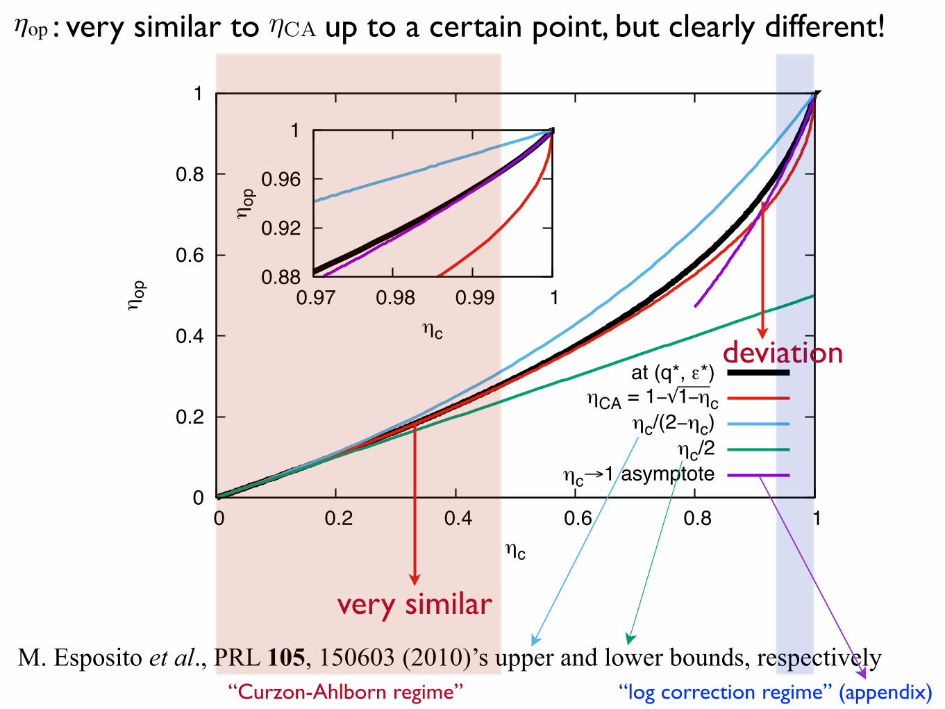
M. Esposito et al., PRL 105, 150603 (2010)’s upper and lower bounds, respectively
deviation
very similar
: very similar to up to a certain point, but clearly different!
“Curzon-Ahlborn regime” “log correction regime” (appendix)
4
0
0.05
0.1
0.15
0.2
0 0.2 0.4 0.6 0.8 1
q* a
nd ε*
ηc = 1 − T2 / T1
q*ε*
q*(ηc→0) = ε*(ηc→0)q*(ηc=1)
ηc→1 asymptote
FIG. 3. Numerically found q
⇤ and ✏⇤ values satisfying Eq. (18), as afunction of ⌘
C
= 1�T2/T1, along with the q
⇤(⌘C
! 0) = ✏⇤(⌘C
! 0)and q
⇤(⌘C
= 1) values presented in Sec. III B 2. ✏⇤(⌘C
= 1) = 0 (thehorizontal axis). The ⌘
C
! 1 asymptote indicates Eq. (34).schematically . . .
�
q
� = q
no net work
as �C is increased
q�(�C � 0) = ��(�C � 0) � 0.083 221 720 199 517 7
q�(�C = 1) � 0.217 811 705 719 800��(�C = 1) = 0
FIG. 4. Illustration of the optimal transition rates (q⇤, ✏⇤) for the max-imum power output as the T2/T1 value varies.
2. Asymptotic behaviors obtained from series expansion
The upper bound for q
⇤ is given by the condition ⌘C
= 1,satisfying ln[(1 � q
⇤)/q⇤] = 1/(1 � q
⇤) and q
⇤(⌘C
= 1) '0.217 811 705 719 800 found numerically and ✏⇤(⌘
C
= 1) = 0exactly from Eq. (16b). ⌘
C
= 0 always satisfies Eq. (18) re-gardless of q
⇤ values, so finding the optimal q
⇤ is meaningless(in fact, when ⌘
C
= 0, the operating regime for the engineis shrunk to the line q = ✏ and there cannot be any positivework). Therefore, let us examine the case ⌘
C
' 0 using theseries expansion of q
⇤ with respect to ⌘C
, as
q
⇤ = q0 + a1⌘C
+ a2⌘2C
+ a3⌘3C
+ O⇣⌘4
C
⌘. (22)
Substituting Eq. (22) into Eq. (18) and expanding the left-handside with respect to ⌘
C
again, we obtain
2 � (1 � 2q0) ln[(1 � q0)/q0]2q0 � 1
⌘C
+q0(1 � q0) � 2a1(1 � 2q0)
2(1 � q0)q0(1 � 2q0)3 ⌘2C
+ c3(q0, a1, a2)⌘3C
+ O⇣⌘4
C
⌘= 0 ,
(23)
where c3(q0, a1, a2) = [10q
60 + 3a
21 � 6q0(a2
1 + a2) � 6q
50(5 +
6a1+8a2)�12q
30(1+6a1+16a
21+9a2)+q
20(1+18a1+132a
21+
42a2)+q
40(31+90a1+96a
21+120a2)]/[6(1�2q0)5(1�q0)2
q
20].
Letting the linear coe�cient to be zero yields
21 � 2q0
= ln
1 � q0
q0
!, (24)
from which the lower bound for q
⇤(⌘C
! 0) = q0 =✏⇤(⌘
C
! 0) ' 0.083 221 720 199 517 7 found numerically[lim⌘
C
!0 U(⌘C
, q⇤) = 1 � 2q
⇤, thus ✏⇤(⌘C
! 0) = q
⇤(⌘C
! 0)by Eq. (16b)]. Figure 3 shows the numerical solution (q⇤, ✏⇤)as a function of ⌘
C
, where the asymptotic behaviors derivedabove hold when ⌘
C
' 0 and ⌘C
' 1. It seems that q
⇤ ismonotonically increased and ✏⇤ is monotonically decreased,as ⌘
C
is increased, i.e., q
⇤min = q
⇤(⌘C
! 0), q
⇤max = q
⇤(⌘C
= 1),✏⇤min = 0, and ✏⇤max = ✏
⇤(⌘C
! 0). Figure 4 illustrates the situ-ation on the (q, ✏) plane. The linear coe�cient a1 in Eq. (22)can be written in terms of q0 when we let the coe�cient of thequadratic term in Eq. (23) to be zero, as
a1 =q0(1 � q0)2(1 � 2q0)
. (25)
Similarly, the coe�cient a2 in Eq. (22) can also be written interms of q0 alone, by letting c3(q0, a1, a2) = 0 in Eq. (23) andusing the relations in Eqs. (24) and (25), as
a2 =7q0(1 � q0)24(1 � 2q0)
. (26)
With the relations of coe�cients in hand, we find theasymptotic behavior of ⌘op in Eq. (19) by expanding it withrespect to ⌘
C
after substituting q
⇤ as the series expansion of⌘
C
in Eq. (22). Then,
⌘op =1
(1 � 2q0) ln[(1 � q0)/q0]⌘
C
+
a1q0�3q
20+2q
30+
[q20+2a1�q0(1+4a1)] ln[(1�q0)/q0]
(1�2q0)3
ln2[(1 � q0)/q0]⌘2
C
+ d3(q0, a1, a2)⌘3C
+ O⇣⌘4
C
⌘,
(27)
where d3(q0, a1, a2) = {2(1 � 2q0)2a1[q2
0 + 2a1 � q0(1 +4a1)] ln[(1�q0)/q0]+2[�2q
40+a1�4a
21�2a2+4q0(4a
21+3a2)+
4q
30(1+a1+4a2)�2q
20(1+3a1+8a
21+12a2)] ln2[(1�q0)/q0]+(1�
2q0)4{�2a
21+[(1�2q0)a2
1�2(1�q0)q0a2] ln[(1�q0)/q0]}}/[(1�q
20)2
q
20]. Using Eqs. (24), (25) and (26), Eq. (27) becomes sim-
ply
⌘op =12⌘
C
+18⌘2
C
+7 � 24q0 + 24q
20
96(1 � 2q0)2 ⌘3C
+ O⇣⌘4
C
⌘. (28)cf) ⌘CA = 1�
p1� ⌘C =
1
2⌘C +
1
8⌘2C +
1
16⌘3C +
5
128⌘4C +O(⌘5C)
Summary and future outlook
Thank you for your attention!!!
• our simple two-level heat engine model: non-Chambadal-Novikov-Curzon-Ahlborn efficiency for the maximum power output• deviation from the third order term: “universal” linear and
quadratic terms• consistent with the equivalent condition for the CNCA
efficiency in terms of the entropy production: J.-M. Park, H.-M. Chun, and J. D. Noh, Phys. Rev. E 94, 012127 (2016).
• ongoing work• 📝 • how universal can our model’s efficiency be, if we modify
the setting? e.g., three-level system: no simple decoupling• implication of ?• taking account quantum effects?
⌘op
(⌘C) � ⌘CA
(⌘C)