Electrical Power and Energy Systems 54 (2014) 306–314

Contents lists available at ScienceDirect

Electrical Power and Energy Systems

journal homepage: www.elsevier .com/locate / i jepes

Optimal power flow solution of wind integrated power system usingmodified bacteria foraging algorithm

0142-0615/$ - see front matter � 2013 Elsevier Ltd. All rights reserved.http://dx.doi.org/10.1016/j.ijepes.2013.07.018

⇑ Corresponding author. Tel.: +91 9861041031.E-mail addresses: ambarish101@gmail.com (A. Panda), manish_tripathy@

yahoo.co.in (M. Tripathy).

Ambarish Panda, M. Tripathy ⇑Department of Electrical Engineering, Veer Surendra Sai University of Technology, Burla, Odisha, India

a r t i c l e i n f o

Article history:Received 19 February 2013Received in revised form 27 June 2013Accepted 13 July 2013

Keywords:Optimal power flowWind energy conversion systemBacteria foraging algorithmDoubly fed induction generator

a b s t r a c t

Owing to the intermittent nature of wind flow, optimal power flow in a power system with considerablewind energy penetration is a challenging issue. In this paper an OPF solution is proposed for IEEE 30 buspower system modified by replacing three conventional generators with equivalent wind energy conver-sion systems (WECS).The uncertain nature of wind power has the risk of over or under estimating thecapacity of available wind power. This uncertainty has been suitably modeled and included in the OPFframework. Moreover, to justify the limitation of reactive power generation capability of doubly fedinduction generator based WECS during under estimation, additional cost component corresponding toexternal reactive power (Q) generating sources has been added in the objective function. The schedulingproblem of WECS integrated power system is solved by formulating it as an optimization problem.Genetic algorithm and a modified bacteria foraging algorithm are employed separately to determinethe optimal schedule. The optimal solution obtained with a modified version of BFA has been found togive better results compared to GA. The results depict the impact of wind and thermal scheduling on totalsystem cost and reiterate the need of additional support of reactive power resources to maintain stablevoltage profiles of the wind–thermal system.

� 2013 Elsevier Ltd. All rights reserved.

1. Introduction

The global electrical energy consumption is rising there byincreasing the demand of power generation. In this scenario, theuse of renewable energy resources like wind power has becomenecessary. Conventionally, the scheduling of generators is carriedout based on economic criteria. Besides economic criteria, decisionregarding the scheduling of generators in an OPF framework [1]plays a vital role. Due to the variable nature of wind, it cannot beassured that the scheduled power from WECS will match withthe power available from wind energy. Therefore, in wind inte-grated systems, the nature of wind makes the above problem tobe different in its modeling. In order to manage the uncertaintyof wind power in the scheduling problem, additional cost compo-nents need to be added. Additional penalty and reserve costs havebeen considered to account for under and over estimation of avail-able wind power [2]. Authors in [3] have discussed the impact ofstochastic nature of wind on overall system operational cost. Theprocess to develop wind farm model and its integration to conven-tional power system has been discussed in [4]. In [5], various costcomponents of wind integrated power system is presented. Addi-

tionally, authors in [6,7] have sought to forecast wind speed andpower using fuzzy logic and neural network respectively. In [8],Cailliau et al. have presented methodology to operate the systemin a secured manner in the presence of increased stochastic windpower generation. Similarly, the authors in [9–11] have demon-strated that apart from modeling the uncertainties of wind, whenvarious operational constraints of the conventional system are re-quired to be included in an OPF formulation, physical limitations ofWECS cannot be ignored. In another work [13], research has shownthat during under estimation, the reactive power (Q) capability ofdoubly fed induction generator (DFIG) may limit the system’s abil-ity to maintain nominal grid bus voltage. To address the securityconcerns in the system, the authors in [13] have formulated a secu-rity constrained economic dispatch in DFIG based WECS wherereactive power capability of DFIG [14] has been analyzed. Authorsin [15–17] have tried to incorporate some dynamic issues relatedto grid synchronization of DFIG in variable speed wind generationsystem .In addition to the aspects discussed in [12,13], this pro-posed work has attempted to include an additional cost compo-nent related to the cost involved in reactive power violation inthe system. The above mentioned extra cost is meant for the reac-tive power requirement (Qc) from other local Q-generating sourcesat WECS buses so that the Q-generating capacity of wind farms arenot violated during under estimation of wind power, and it may bepossible to operate the system in a voltage secure manner. In this

A. Panda, M. Tripathy / Electrical Power and Energy Systems 54 (2014) 306–314 307

regards, the total cost in OPF formulation is obtained by adding thetotal conventional generation cost, cost of constraint violation andadditional cost Qc. Evolutionary techniques i.e. genetic algorithm(GA) and a modified bacteria foraging algorithm (BFA) are appliedto optimize the objective functions. The optimized generatingschedules are tested for their ability to operate the system se-curely, when the system is subjected to numbers (N � 1) contin-gencies in the form of line outages. Simulations are carried out inMATLAB/SIMULINK environment.

The paper is organized in the following manner. The main prob-lem is formulated in Section 2. Section 3 discusses about the capa-bility of reactive power in DFIG integrated WECS. Section 4presents a brief overview of optimization techniques applied inthis work. In Section 5, procedural details of simulations and re-sults are presented. In the same section few pertinent observationsare made regarding the results obtained which has led to conclu-sions in Section 6.

2. Problem formulation

2.1. Problem

For satisfactory operation of wind integrated power system,wind power fluctuation must be balanced by other types of gener-ation. The nature of uncertainty of wind emphasizes, that the sys-tem should incorporate additional cost due to power imbalance.Moreover, as discussed earlier the limited capacity of reactivepower of DFIG warrants additional reactive power support at theWECS buses. As these additional costs may prove to be uneconom-ical, therefore their inclusion in the cost function would be morerealistic. Considering this aspect, two types of objective functionsare formulated as presented in (1) and (2) respectively. An addi-tional cost Qc which corresponds to the cost of additional reactivepower resources is added in F2 unlike in F1. The problem is formu-lated as below

Minimize

F1 ¼XNg

t

CtðPgtÞ þXNw

r

½CwrðPwrÞ þ Cp;wrðPwr;av � PwrÞ þ Cr;wrðPwr

� Pwr;avÞ� þ Pf1 þ Pf2 ð1Þ

Minimize

F2 ¼XNg

t

CtðPgtÞ þXNw

r

½CwrðPwrÞ þ CP;wrðPwr;av � PwrÞ þ CR;wrðPwr

� Pwr;avÞ� þ Pf1 þ Pf2 þ Q c ð2Þ

Subject to constraints:

XNg

t

Pgt þXNw

r

Pwr ¼ Ploss þ Pload ð3Þ

XNg

t

Q gt þXNw

r

Q wr ¼ Q loss þ Qload ð4Þ

Pmingt 6 Pgt 6 Pmax

gt ð5Þ

Q mingt 6 Q gt 6 Q max

gt ð6Þ

Vmint 6 Vt 6 Vmax

t ð7Þ

Pwr 6 Pmaxwr ð8Þ

Q minwr 6 Q wr 6 Q max

wr ð9Þ

In the function F1 defined above notations t and g denote the con-ventional (thermal) units and r and w denote the renewable (wind)units. The first and second terms in (1) denote the cost of thermalpower generation and the cost of power purchase from wind powerproducer as defined in (10) and (11) respectively. Similarly, thethird and fourth terms in (1) are the additional costs of under andover estimated wind power components to account for the windpower intermittency [5]. Pf1 and Pf2 are suitable penalty functionsto consider the effect of additional cost required to operate the sys-tem within the physical constraints. Details of the above terms arepresented in the following sub-sections.

2.2. Evaluation of cost of thermal generating units

Widely acclaimed quadratic cost function for thermal genera-tors are adopted which is explained by (10) as follows

CtðPgtÞ ¼ atP2gt þ btPgt þ ct ð10Þ

Where at, bt, ct are the cost coefficients of tth thermal unit and Pgt isthe power output of tth generator. These are specified in Table 1.

2.3. Evaluation of direct cost

The cost of purchase of wind power from wind power produceris termed as the direct cost and is expressed in (11) as the follows

CwrðPwrÞ ¼ drPwr ð11Þ

where dr is the direct cost coefficient of the rth wind generator andPwr is the scheduled power output of rth wind unit.

2.4. Evaluation of cost corresponding to surplus wind power

When the scheduled power is found to be less than the capacityof actual wind power available, the scenario is known as under esti-mation. During underestimation, there will be a surplus amount ofavailable wind power. From the system operation point of view,the ISO should maximize the utilization of available wind power.It can be done by reducing the power output of conventional gen-erators by fast re-dispatch and automatic generation control. In thecase when it is not feasible then ISO has to pay an equivalent costto the wind power producer (WPP) for not utilizing all availablewind resources. The above cost is termed as penalty cost, whichcan be represented as follows

Cp;wrðPwr;av � PwrÞ ¼ KPrðPwav � PwrÞ

¼ Kpr

Z Pro

Pwr

ðw� PwrÞfwðwÞdw ð12Þ

KPr is the penalty cost coefficient for the rth wind generator andfw(w) WECS wind power probability density function (PDF) [18].In order to model and characterize the wind speed suitably and toconvert it into wind power, Weibull distribution function [18,19]has been used in this work. Pwr, Pro, Pwav are respectively the sched-uled, rated power and available wind power from rth wind poweredgenerator.

2.5. Evaluation of cost corresponding to deficit wind power

There may be situations when the actual available wind powercould fall behind the scheduled value. The scenario is referred asover estimation. During this situation, in order to meet the load de-mand and to compensate the differential amount, some reserveunits’ need to be committed by the ISO. The cost of committingthe reserve generating units to meet the wind power shortage iscalled the reserve cost. The cost as a function of power can be rep-resented as follows

308 A. Panda, M. Tripathy / Electrical Power and Energy Systems 54 (2014) 306–314

CRwrðPwr � PwravÞ ¼ KRrðPwr � PwavÞ

¼ KRr

Z Pwr

0ðPwr �wÞfwðwÞdw ð13Þ

KRr is the reserve cost coefficient of rth wind generator and CRwr isthe reserve cost of Pwr.

2.6. Penalty functions for constraint violation

In order to obtain a constrained optimization solution of theobjective function defined in (1), the inequality constraints for realpower line flow and bus voltage limits are incorporated as penaltyfunctions represented as Pf1 and Pf2. Their mathematical expres-sions are

Pf1 ¼ abs½signðPmax � PkÞ � 1��pf

þ abs½signðPmin � PkÞ þ 1��pf ð14Þ

Pf2 ¼ abs½1þ signðVk � VmaxÞ��pf

þ abs½1� signðVk � VminÞ��pf ð15Þ

In (14) Pmax and Pmin denote the maximum and minimum limitingvalues of real power and Pk is the actual magnitude of real powerfor the kth line under consideration. Similarly in (15), Vk is the volt-age magnitude of the kth bus where as Vmin and Vmax are the mini-mum and maximum values among the bus voltages respectively. In(14), as long as Pk, lies within Pmax and Pmin, Pf1 has a value equal tozero. Depending upon the direction of violation i.e. whether maxi-mum or minimum limit is violated, either the first or the secondpart of the penalty function in expression (14) becomes a high po-sitive valued cost which penalizes the total cost. Similar explanationalso holds good for (15) which defines the penalty function for volt-age violation.

2.7. Evaluation of cost corresponding to reactive power management

The terms described from Section 2.2 to 2.6 are common in boththe functions F1 and F2. But the additional term Qc added in F2,which accounts for the reactive power violation cost in DFIG, is ex-plained as follows.

As there are possibilities of degradation of bus voltage profileduring under estimation scenario due to limited Q generating capa-bilities of DFIGs, necessary reactive power support has to bebrought from local Q generating sources, which can mitigate thereactive power violation (Qvio) of DFIG units and alleviate the deg-radation of their bus voltages. Evaluation of Qvio requires the con-sideration of the capability limit of DFIG systems. MathematicallyQvio is represented by the following equation

Qvio ¼ abs sign Q speclimit � Q calc

� �h ið16Þ

Q c ¼ KcQvio ð17Þ

Here Qspeclimit denotes the limiting values of specified reactive power of

the thermal units which are being replaced by WECS. Limiting valueindicates that it may be one among the minimum or maximum val-ues of Qlimit. However, Qcalc is the calculated value of reactive powerof the DFIG grid side converter (GSC) that depends upon the currentand voltage ratings of the converter. Kc is the cost coefficient usedfor the calculation of Qc. More detail discussions about the Q-gener-ating limit in DFIG systems is presented in Section 3.

2.8. Modeling of wind speed variability

Physical methods and statistical data have certain limitation inpredicting the highly stochastic nature of wind speed, so investiga-

tions were focussed on finding a specific distribution [18] whichwill fit more accurately to the randomness in wind speed. In thiswork the widely used distribution function known as WeibullPDF has been used to model and characterize the variability ofwind. Mathematically it is represented by

fvðvÞ ¼kc

� �vc

� �ðk�1Þe�

vcð Þk ;0 < v <1 ð18Þ

Here c is the scale parameter which indicates the random variationof wind and has the unit same as wind speed. Similarly k is theshape parameter which gives the shape of mean wind speed (v) pro-file and is a dimensionless quantity.

3. Reactive power capability of DFIG

In order to examine the affects of wind variation on the sched-uling problem it is required that the real and reactive power capa-bility characteristics of DFIG systems [13,14] be understood at theoutset. The converter systems and particularly the GSC, whichoperates with power electronics switches has power limitationsand thus fix the limits of generator’s real and reactive power capac-ities. During under estimation, as the systems available windpower becomes more than the value required to be scheduled,therefore the Q generating capacity of DFIG system reduces. Tounderstand the operation more clearly it is essential to know themodeling of DFIG in d–q reference frame which is derived frominduction motor model [27]. In most of the control strategies ofDFIG, the rotor side converter (RSC) controls the real and reactivepower by varying the rotor current components while the GSC con-trols the DC link voltage and ensures converter operation at unitypower factor. Also the operation of wind turbine as a prime moverwith DFIG control attributes has been reported in [26,28]. Theinstantaneous values of real and reactive powers of the DFIG sys-tem expressed in terms of stator and rotor voltages and currentsmay be represented as follows

vds ¼ �Rsids þxs½ðLs þ LmÞiqs þ Lmiqr� ð19Þ

vqs ¼ �Rsiqs �xs½ðLs þ LmÞids þ Lmidr� ð20Þ

vdr ¼ �Rridr þ sxs½ðLr þ LmÞiqr þ Lmiqs� ð21Þ

vqr ¼ �Rriqr � sxs½ðLr þ LmÞidr þ Lmids� ð22Þ

P ¼ Ps þ Pr ¼ vdsids þ vqsiqs þ vdridr þ vqriqr ð23Þ

Q ¼ Q s þ Q r ¼ vqsids � vdsiqs þ vqridr � vdriqr ð24Þ

In the above expression subscript s stands for stator side quantityand r stands for rotor side quantities and subscript d and q standfor direct and quadrature axis components respectively. xs is thesynchronous speed. Rs, Ls are the stator resistance and self induc-tance. Rr, Lr denotes the rotor resistance and self inductance andLm is the magnetizing inductance of DFIG. P and Q are the realand reactive power supplied by the DFIG. Neglecting the statorresistance it is assumed that d-axis coincides with the maximumstator flux, thus making mqs equal to the stator terminal voltage.The rotor current can be expressed as

Ir ¼ffiffiffiffiffiffiffiffiffiffiffiffiffiffiffiffii2dr þ i2

qr

qð25Þ

In DFIG systems the reactive power required by the stator (Qs) isdelivered by the GSC. Therefore, lower and upper bounds of reactivepower generating capacities of GSC would limit the capability ofDFIG system to supply Qs. However, the GSC is power electronicsbased converter and it has physical limitation in terms of itsKVA or current rating. This may influence the optimal solution of

A. Panda, M. Tripathy / Electrical Power and Energy Systems 54 (2014) 306–314 309

scheduling. In order to determine the upper and lower bounds of Qs

the following approach is adopted. In the d–q frame of reference, theq axis is aligned with the grid voltage vector resulting in vds equals tozero. Thus considering the maximum stator current limitation andsubstituting vqs equal to vs, along with zero value for vds in (23) and(24) the stator active power and reactive power may be expressed as

Ps ¼ vqsiqs ð26Þ

Q s ¼ vqsids ð27Þ

From (27) it can be observed that Qs is dependent on direct axiscomponent of stator current ids. Further, maintaining the stator volt-age vs (equal to vqs) at 1p.u, the range of Qs between sub-synchro-nous to super-synchronous modes can be expressed asffiffiffiffiffiffiffiffiffiffiffiffiffiffiffiffiffiffiffiffiffiffiffiffiffiffi

Imax2

s � i2qs

� �r6 Q s 6

ffiffiffiffiffiffiffiffiffiffiffiffiffiffiffiffiffiffiffiffiffiffiffiffiffiffiImax2

s þ i2qs

� �rð28Þ

where Imaxs is the maximum capacity of stator current. Moreover

finding ids from (20) and putting in (27) the reactive power ex-changed with the grid at the stator terminal is represented as

Q s ¼ �v2

qs

xsðLs þ LmÞ� Lmvqsidr

Ls þ Lmð29Þ

In the above equation the magnetization of the stator is representedby the first term where as the second term represents the net reactivepower exchanged with the grid. It can be observed from (29) that thereactive power is controlled by idr. Therefore a strong dependency canbe witnessed between Qs and idr. Substituting (26) in (19), the quad-rature axis component of rotor current is obtained as

iqr ¼ �PsðLs þ LmÞ

LmVqsð30Þ

Under maximum rotor current limitation constrained by GSC’smaximum current rating imax

r , idr may be expressed as

idr ¼ffiffiffiffiffiffiffiffiffiffiffiffiffiffiffiffiffiffiffiffiffiffiffiffiffiffiimax2

r � i2qr

� �rð31Þ

Finally, substituting the values of iqr and idr from (30) and (31) in(29), the upper and lower limit of reactive power of the DFIG undermaximum rotor current can be expressed as

0 0.2 0.4 0.6 0.82060

2070

2080

2090

2100

2110

2120

2130

2140

2150

2160

No of g

cost

Convergenc

Fig. 1. Convergence characteristics of Scen

Qs P � v2s

xsðLs þ LmÞ� Lmvs

ðLs þ LmÞ

ffiffiffiffiffiffiffiffiffiffiffiffiffiffiffiffiffiffiffiffiffiffiffiffiffiffiffiffiffiffiffiffiffiffiffiffiffiffiffiffiffiffiffiffiffiffiimax2

r � PsðLs þ LmÞv sLm

� �2s

ð32Þ

Qs 6 �v2

s

xsðLs þ LmÞþ Lmvs

ðLs þ LmÞ

ffiffiffiffiffiffiffiffiffiffiffiffiffiffiffiffiffiffiffiffiffiffiffiffiffiffiffiffiffiffiffiffiffiffiffiffiffiffiffiffiffiffiffiffiffiffiimax2

r � PsðLs þ LmÞv sLm

� �2s

ð33Þ

Considering above formulation, Qvio defined earlier in (16), is evalu-ated in the following manner. Initial assumption is made where min-imum and maximum limits of WECS are kept equal to the Q limitsspecified in [20]. However the GSC of the DFIG based WECS has itsown limiting capabilities of reactive power as specified in Eqs. (32)and (33). Therefore, while solving the power flow, it should be seenthat the net Q supplied by DFIG should lie within the specifiedbounds. This can be achieved if load flow solution is repeated itera-tively till a solution is obtained which stays within Qmax and Qmin ofDFIG as given by (32) and (33). If the solution is sought followingthe above procedure, then after few iterations the Qvio should fall tozero and in that case the objective function would be F1. Howeverwith the objective function F2, no iterative solution is adopted, asthe cost of additional Q support by external means, which is equalto Qvio is added with it. In this case, the voltages are left uncorrected.

In order to quantify the net bus voltage violations from theirrespective nominal values during (N � 1) contingencies a voltageviolation index (VVI) is evaluated by comparing the bus voltageprofiles before and after different line outage cases

VVI ¼XN

n¼1

Vn �XN

n¼1

VOUTn ð34Þ

In the above expression Vn is the nominal bus voltage of the nth busprior to a line outage case. VOUT

n is the bus voltage of the correspond-ing bus obtained after the outage case. N is the total number of P–Qbuses present in the system.

4. Brief overview of optimization methodologies

For the purpose of optimization GA and BFA are employed tooptimize both the objective functions and their respective perfor-mances are compared. Brief overviews of both the algorithms arediscussed below.

1 1.2 1.4 1.6 1.8 2

x 104enerations

e characteristics

BFAGA

ario1 with changed set of parameters.

0.2 0.4 0.6 0.8 1 1.2 1.4 1.6 1.8 2

x 104

2060

2070

2080

2090

2100

2110

2120

2130

2140

2150

2160

No of generation

Cos

t

Convergence characteristics

BFAGA

Fig. 2. Convergence characteristics of Scenario2 with changed set of parameters.

310 A. Panda, M. Tripathy / Electrical Power and Energy Systems 54 (2014) 306–314

4.1. Genetic algorithm

Genetic algorithm (GA) [24] is an established parallel searchalgorithm, which has been applied in varieties of optimizationproblems in power systems. In GA, the initial set of randomly gen-erated population evolves through several generations to repro-duce fitter candidate solutions using crossover and mutationoperators. As the algorithm is based on idea of the survival of thefittest, the weaker off-springs get eliminated. During the searchprocess, as there is no restriction on the search space, it enhancesthe robustness of GA.

4.2. Bacteria foraging algorithm

BF algorithm is an efficient population based stochastic searchtechnique recently developed by Passino [23]. In recent years, BFhas been applied in solving numbers of optimization problems inpower systems [21,25] due to its ability to search the promisingareas of the solution space. The idea of BF algorithm is based onthe foraging mechanism of E. coli bacteria present in human intes-tines. During foraging of the real bacterium, locomotion is achievedby a set of tensile flagella. Flagella help an E. coli bacterium to tum-ble or swim, which are two basic operations performed by a bacte-rium at the time of foraging. When they rotate the flagella in theclockwise direction, each flagellum pulls on the cell. This resultsin the moving of flagella independently and finally the bacteriumtumbles less frequently. Alternatively, in a harmful place it tum-bles frequently to find a nutrient gradient. The four different stepsof this algorithm are chemo taxis, swarming, reproduction andelimination and dispersion. The details of the algorithm steps canbe referred from [22], where the original version of the algorithmproposed in [23] is modified inside both chemotaxis and swarmingstages. The proposed modifications which expedite the conver-gence are also applied in this work. Two major modification pointsadopted in this improved version of BFA are summarized below.

(1) For a minimization problem, instead of taking the average ofall the chemotactic stage cost functions [23], the minimumvalue of cost function obtained for each bacterium in thechemotactic stages, is retained before sorting is done forreproduction.

(2) For swarming, the distances of all the bacteria in a new che-motactic stage is evaluated from the optimum bacterium tillthat point of solution and not by the distances of all the bac-teria from rest others as suggested in [23].

The flow chart of the algorithm with above modifications is gi-ven in Fig. A3 in the Appendix.

5. Simulation results and discussion

For simulation of the work, the IEEE-30 bus system [20] is con-sidered. The system is modified by replacing conventional genera-tors with wind farms located at fifth, eleventh and thirteenth bus.Each wind farm (WF) consists of several wind turbine generators(WTG) equipped with DFIGs. In this work, WF at bus No. 5 consistsof ten WTG (each of 5 MW) having a total capacity of 50 MW. Sim-ilarly WF at bus numbers 11 and 13 each consist of ten WTG of4 MW capacities with a total capacity of 40 MW. The optimizationof two different objective functions as defined in (1) and (2) is car-ried out with the help of BFA and GA separately.

5.1. Optimal cost evaluation

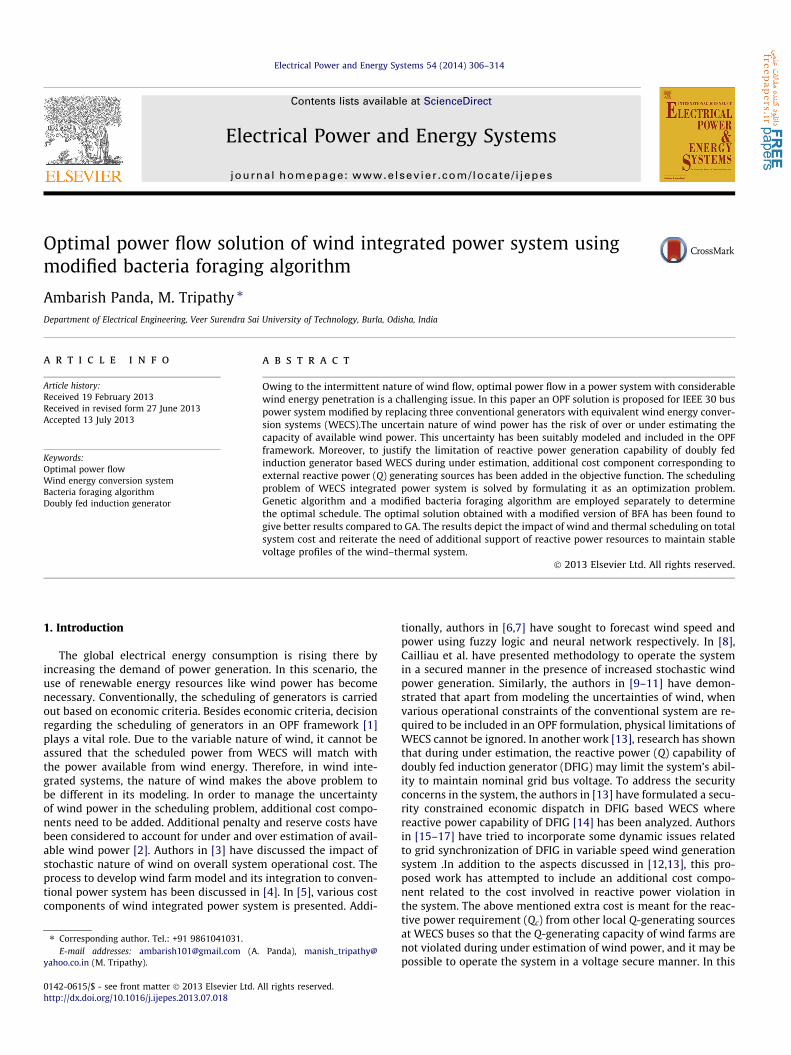
Before discussing the results in both the algorithms, two differ-ent scenarios of power flow cases need to be defined. In, Scenario-1, the power flow solution tries to limit the Qvio to zero, where as inScenario-2 power flow seeks a solution where Qvio is not restricted.Some more details on both these scenarios are discussed in Sec-tions 5.1.1 and 5.1.2 respectively, where optimal cost of generationafter choosing the best possible control parameters (mentioned inAppendix A.3), is evaluated under two scenarios presented. In boththe algorithms, randomly generated numbers are suitably scaledup to represent a set of real power generation schedule of boththermal and wind systems. Each such potential solution is termedas a bacterium in case of BFA and an individual in the population ofGA. Along with this, to observe the effect of variation in controlparameters used in BFA and GA on the optimal solution conver-gence characteristics are obtained with various sets of parameters.Two such sample convergence characteristics are shown in Figs. 1and 2 for scenario1 and scenario2 respectively. The corresponding

Table 1Cost coefficients of thermal generating units.

Generator no Cost coefficients Min limit (MW) Max limit (MW)

at bt ct

1 0.00975 2.5 0 50 2002 0.0175 1.75 0 20 803 0.0625 1.0 0 10 40

0.5 1 1.5 2 2.5x 10

4

2060

2070

2080

2090

2100

2110

2120

2130

Optimization Curve

No of generation

Cos

t

GABFA

0.5 1 1.5 2

x 104

2070

2080

2090

2100

Fig. 3. Convergence characteristics of BFA and GA for Scenario-1.

Table 2Optimized generation schedule of the generators in p.u. obtained with BFA and GAduring Scenario-1.

Scenario-1

BFA GA

Pg Q Pg Q

1 0.5926 1.0705 0.5946 1.07052 0.6170 �0.3270 0.6200 �0.32755 0.4880 �0.0012 0.5000 �0.00128 0.3800 �0.4500 0.4000 �0.450011 0.4000 0.2489 0.4000 0.249813 0.3780 0.2495 0.3800 0.2501Qvio 0 0CTotal 2062.52 2063.34

0 0.5 1 1.5 2 2.5 3

x 104

2060

2080

2100

2120

2140

2160

2180

2200

No of generation

Cos

t

Optimization Curve

BFAGA

0.5 1 1.5 2 2.5

x 104

2070

2080

2090

2100

2110

2120

Fig. 4. Convergence characteristics of BFA and GA for Scenario-2.

Table 3Optimized generation schedule of the generators in p.u. obtained with BFA and GAduring Scenario-2.

Scenario-2

BFA GA

Pg Q Pg Q

1 0.5826 0.8241 0.5846 0.82452 0.6200 �0.3270 0.6190 �0.32705 0.4992 0.1100 0.5000 0.11088 0.4002 �0.4500 0.4000 �0.455211 0.4001 0.3000 0.4000 0.300013 0.3790 0.3000 0.3800 0.3000Qvio 0.1678 0.1676CTotal 2063.53 2066.2

5 10 15 20 25 300.9

0.92

0.94

0.96

0.98

1

1.02

1.04

1.06

Mag

nitu

de (p

.u)

NominalBFAGA

A. Panda, M. Tripathy / Electrical Power and Energy Systems 54 (2014) 306–314 311

changed sets of parameters are given in the Appendix (A.2). Theconvergence characteristics shows that BFA in Scenario-1 and Sce-nario-2 settles at 2062.71 and 2063.65 respectively while GA con-verged at 2063.54 and 2066.43 with changed parameters. Fromexperience, several such sets of parameters are considered, andthe optimized solutions with each one of them are compared.The optimal solutions obtained for the best set of control parame-ters for both GA and BFA in each scenario are discussed below.

Bus No

Fig. 5. Comparison of voltage profile during outage of line 12–15.

5.1.1. Scenario-1

The total cost of generating power in the wind–thermal systemis evaluated without considering any cost corresponding to localreactive power support. In this case, Qvio as defined in (16) is iter-atively solved and minimised to zero during each run of the loadflow solution. The objective function for this scenario is repre-sented by (1) which is optimized with the help of GA and BFA.The details of parameters chosen with each of the optimization

algorithm are given in the Appendix. Fig. 3 depicts the convergencecharacteristics of BFA and GA respectively. Similarly, Table 2 enu-merates the optimum cost obtained during this scenario. Fromthe result, it may be pointed out that BFA has marginally improvedsolution compared to GA but more importantly the speed of con-vergence is considerably better than GA as shown in Fig. 10.

5 10 15 20 25 300.9

0.92

0.94

0.96

0.98

1

1.02

1.04

1.06

Bus no

Mag

nitu

de (p

.u.)

NominalBFAGA

Fig. 6. Comparison of voltage profile during outage of line 15–23.

5 10 15 20 25 300.88

0.9

0.92

0.94

0.96

0.98

1

1.02

1.04

1.06

1.08

Bus no

Mag

nitu

de (p

.u.)

NominalBFAGA

Fig. 7. Comparison of voltage profile during outage of line 10–20.

5 10 15 20 25 300.9

0.92

0.94

0.96

0.98

1

1.02

1.04

1.06

Bus No

Mag

nitu

de (p

.u.)

NominalBFAGA

Fig. 8. Comparison of voltage profile during outage of line 15–18.

5 10 15 20 25 300.88

0.9

0.92

0.94

0.96

0.98

1

1.02

1.04

1.06

1.08

Bus no

Mag

nitu

de (p

.u.)

NominalBFAGA

Fig. 9. Comparison of voltage profile during outage of line 6–28.

Table 4Comparative performance in terms of voltage violation index.

Sr. no Line outage no Voltage violation index (p.u.)

BFA GA

1 12–15 0.3319 0.36552 10–20 0.4994 0.52873 6–28 0.4007 0.42164 15–23 0.5683 0.61555 15–18 0.5912 0.6372

312 A. Panda, M. Tripathy / Electrical Power and Energy Systems 54 (2014) 306–314

5.1.2. Scenario-2In this scenario, the load flow solution does not limit its solution

according to the KVAR rating of the GSC. Therefore, the require-ment of additional reactive power to be provided by externalsources at the DFIG bus is considered. In the solution of load flow,

the Q-limits at the DFIG buses are kept at their original values asgiven in [20]. Hence, instead of attempting to minimize Qvio anaddition cost component is added to the generation cost, so thatits effect on system parameters and constraints can be analysed.The convergence characteristics obtained with BFA and GA are de-picted in Fig. 4 and the final optimized values of the objective func-tion are given in Table 3.

As observed from Table 3, the optimal cost obtained with BFA inScenario-1 and Scenario-2 are 2062.52 and 2063.53 units, where asthose obtained with GA are 2063.34 and 2066.2 units respectively. Itshows that BFA is giving better solution as compared to GA. FromFigs. 3 and 4, it can be observed that BFA gives superior performanceduring the optimization process compared to GA. Similarly in thisscenario, the speed of convergence is faster in BFA compared to GA.

5.2. System analysis under (N – 1) contingency states

In order to examine the effectiveness of the optimized genera-tion schedule obtained with BFA and GA, in terms of maintainingthe voltage profile in the system, some disturbances in the formof line outages are created in it. The details of such disturbancesand their effects on the system are discussed as follows.

Fig. 5 shows the comparison between the voltage profiles of thesystem when the line 12–15 is taken out of the system. It demon-strates that, variation in the bus voltages is relatively less in BFAthan GA, when compared with nominal bus voltages. The fact isclearly distinguished looking at the post disturbance voltages atbus numbers 18, 19 and 23. Besides this, minor improvements involtage are also observed in bus 5, 7, 10 and 12 buses. In all thesenodes, optimal voltages obtained by BFA are closer to their respec-tive nominal values prior to the outage case.

In order to further probe into the effectiveness of BFA over GA,few more line outage scenario are carried out. More line outageconditions are simulated in the form of lines 15–23, 10–20, 15–18 and 6–28 being removed separately from the system one byone. The voltage profiles obtained for generation schedules withBFA and GA are depicted in Figs. 6–9 respectively. As highlighted

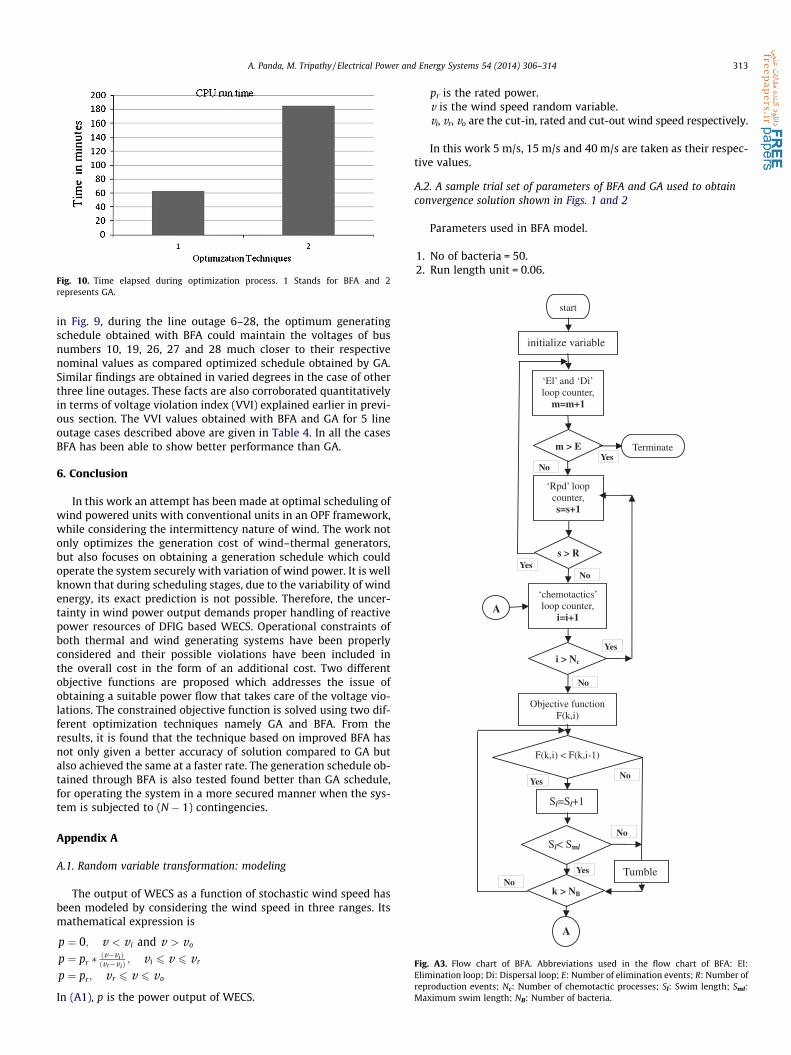
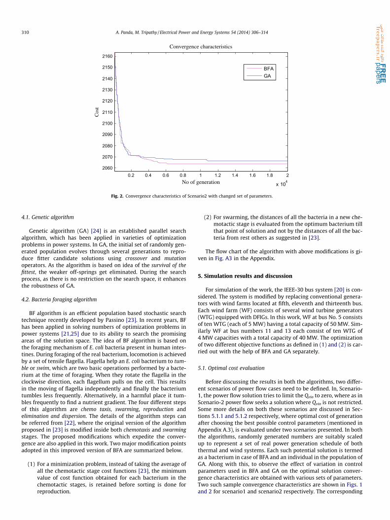
Fig. 10. Time elapsed during optimization process. 1 Stands for BFA and 2represents GA.

Yes No

No

Yes

Yes No

No Yes

Yes

No

No

start

initialize variable

‘El’ and ‘Di’ loop counter,

m=m+1

m > E

‘Rpd’ loop counter, s=s+1

s > R

‘chemotactics’ loop counter,

i=i+1

i > Nc

Terminate

A

Objective function F(k,i)

F(k,i) < F(k,i-1)

Sl=Sl+1

Sl< Sml

k > NB

Tumble

A

Fig. A3. Flow chart of BFA. Abbreviations used in the flow chart of BFA: El:Elimination loop; Di: Dispersal loop; E: Number of elimination events; R: Number ofreproduction events; Nc: Number of chemotactic processes; Sl: Swim length; Sml:Maximum swim length; NB: Number of bacteria.

A. Panda, M. Tripathy / Electrical Power and Energy Systems 54 (2014) 306–314 313

in Fig. 9, during the line outage 6–28, the optimum generatingschedule obtained with BFA could maintain the voltages of busnumbers 10, 19, 26, 27 and 28 much closer to their respectivenominal values as compared optimized schedule obtained by GA.Similar findings are obtained in varied degrees in the case of otherthree line outages. These facts are also corroborated quantitativelyin terms of voltage violation index (VVI) explained earlier in previ-ous section. The VVI values obtained with BFA and GA for 5 lineoutage cases described above are given in Table 4. In all the casesBFA has been able to show better performance than GA.

6. Conclusion

In this work an attempt has been made at optimal scheduling ofwind powered units with conventional units in an OPF framework,while considering the intermittency nature of wind. The work notonly optimizes the generation cost of wind–thermal generators,but also focuses on obtaining a generation schedule which couldoperate the system securely with variation of wind power. It is wellknown that during scheduling stages, due to the variability of windenergy, its exact prediction is not possible. Therefore, the uncer-tainty in wind power output demands proper handling of reactivepower resources of DFIG based WECS. Operational constraints ofboth thermal and wind generating systems have been properlyconsidered and their possible violations have been included inthe overall cost in the form of an additional cost. Two differentobjective functions are proposed which addresses the issue ofobtaining a suitable power flow that takes care of the voltage vio-lations. The constrained objective function is solved using two dif-ferent optimization techniques namely GA and BFA. From theresults, it is found that the technique based on improved BFA hasnot only given a better accuracy of solution compared to GA butalso achieved the same at a faster rate. The generation schedule ob-tained through BFA is also tested found better than GA schedule,for operating the system in a more secured manner when the sys-tem is subjected to (N � 1) contingencies.

Appendix A

A.1. Random variable transformation: modeling

The output of WECS as a function of stochastic wind speed hasbeen modeled by considering the wind speed in three ranges. Itsmathematical expression is

p ¼ 0; v < v i and v > vo

p ¼ pr � ðv�v iÞðvr�v iÞ

; v i 6 v 6 v r

p ¼ pr; v r 6 v 6 vo

In (A1), p is the power output of WECS.

pr is the rated power.v is the wind speed random variable.vi, vr, vo are the cut-in, rated and cut-out wind speed respectively.

In this work 5 m/s, 15 m/s and 40 m/s are taken as their respec-tive values.

A.2. A sample trial set of parameters of BFA and GA used to obtainconvergence solution shown in Figs. 1 and 2

Parameters used in BFA model.

1. No of bacteria = 50.2. Run length unit = 0.06.

314 A. Panda, M. Tripathy / Electrical Power and Energy Systems 54 (2014) 306–314

3. No of chemotactic step = 4.4. Magnitude of attractant by a bacterium = 1.08.5. Probability of elimination of bacteria = 0.25.

Parameters used in GA model.

1. No of individual in population = 75.2. Probability of crossover = 0.87.3. Probability of mutation = 0.03.

A.3. Best set of parameters of BFA and GA finally used to obtainconvergence solution shown in Figs. 3 and 4

Parameters used in BFA model.

1. No of bacteria = 40.2. Run length unit = 0.04.3. No of chemotactic step = 4.4. Magnitude of attractant by a bacterium = 1.08.5. Probability of elimination of bacteria = 0.25.

Parameters used in GA model.

1. No of individual in population = 95.2. Probability of crossover = 0.85.3. Probability of mutation = 0.05.

(see Fig. A3)

References

[1] Carpentier J. Optimal power flows. Int J Electr Power Energy Syst 1979;1:3–15.[2] Jabr RA, Pal BC. Intermittent wind generation in optimal power flow

dispatching. IET Gener Transm Distrib 2009;3(1):66–74.[3] Miguel A, Vazquez O, Kirschen DS. Accessing the impacts of wind power

generation on operating cost. IEEE Trans Smart Grid 2010;1(3):295–301.[4] Heras IS, Escriva GS, Ortega MA. Wind farm electrical power production model

for load flow analysis. Renew Energy. Elsevier; 2011. vol. 36, p. 1008–13.[5] Hetzer J, Yu DC, Bhattarai K. An economic dispatch model incorporating wind

power. IEEE Trans Energy Convers 2008;23(2):603–11.[6] Damousis IG, Alexiadis MC, Theocharis JB. A fuzzy model for wind speed

prediction and power generation in wind parks using spatial correlation. IEEETrans Energy Convers 2004;19(2):352–61.

[7] Li S, Wunsch DC, O’Hair EA, Giesselmann MG. Using neural networks toestimate wind turbine power generation. IEEE Trans Energy Convers2001;16(3):276–82.

[8] Cailliau M, Foresti M, Villar CM. Winds of change. IEEE Power Energy Magn2010;8(5):52–62.

[9] Chen H, Chen J, Duan X. Multi-stage dynamic optimal power flow in windpower integrated system. IEEE/PES Transmis Distrib Conf Exhibit 2005:1–5.

[10] Chen CL, Lee TY, Jan RM. Optimal wind–thermal coordination dispatch inisolated power systems with large integration of wind capacity. EnergyConvers Manage 2006;47(18–19):3456–72.

[11] Bratcu AI, Munteanu I, Ceanga E.Optimal control of wind energy conversionsystems: from energy optimization to multipurpose criteria-a short survey. In:16th Mediterranean conference on control and automation. Ajaccio, France;2008.

[12] Pena R, Clare JC, Asher GM. A doubly fed induction generator using back toback PWM converters supplying an isolated load from a variable speed windturbine. IEEE Proc Electr Power Appl 1996;I43(5):380–7.

[13] Mishra S, Mishra Y, Vigness S. Security constrained economic dispatchconsidering wind energy conversion systems. IEEE/PES Conf 2011.

[14] Engelhardt S, Erlich I, Feltes C, et al. Reactive power capability of wind turbinesbased on doubly fed induction generators. IEEE Trans Energy Convers2011;26(1):364–72.

[15] Ahmed G, Abo K. Synchronization of DFIG output voltage to utility grid in windpower system. Renew Energy. Elsevier; 2012. vol. 44, p. 193–8.

[16] Gomez SA, Amenedo JLR. Grid synchronization of doubly fed inductiongenerators using direct torque control. IEEE IECON Conf Proc 2002;4:3338–43.

[17] Chen SZ, Cheung NC, Zhang Y, et al. Improved grid synchronization control ofdoubly fed induction generator under unbalanced grid voltage. IEEE TransEnergy Convers 2011;26(3):799–810.

[18] Tsikalakis AG, Katsigiannis YA, Georgilakis PS, Hatziargyriou ND. Determiningand exploiting the distribution function of wind power forecasting error forthe economic operation of autonomous power system. IEEE Power Eng SocGener Meet 2006.

[19] Seguro JV, Lambert TW. Modern estimation of the parameters of the Weibullwind speed distribution for wind energy analysis. J Wind Eng Ind Aerodyn2000;85(15-84).

[20] Pai MA. Computer methods in power system analysis. TMH Publishers; 1996.[21] Tripathy M, Mishra S, Nanda J. Multi machine power system stabilizer design

by rule based bacteria foraging. Electr Power Syst Res 2007;77(2):1595–607.[22] Tripathy M, Mishra S. Bacteria foraging based solution to optimize both real

power loss and voltage stability limit. IEEE Trans Power Syst2007;22(1):240–8.

[23] Passino KM. Biomimicry of bacterial foraging for distributed optimization andcontrol. IEEE Control Syst Magn 2002;22(3):52–67.

[24] Abdel-Magid YL, Abido MA, Al-Baiyat S, Mantawy AH. Simultaneousstabilization of multimachine stabilizers via genetic algorithm. IEEE TransPower Syst 1999;14:1428–39.

[25] Ali ES, Abd-Elazim SM. Bacteria foraging optimization algorithm based loadfrequency controller for interconnected power system. Elect. Power andEnergy Systems, Elsevier 2011;33(3):633–8.

[26] Oshaba AS, Ali ES. Speed control of induction motor fed from wind turbine viapso based PI controller. Int.Research Journal of Applied Science, Engg andTechnology 2013;5(18):4594–606.

[27] Kundur P. Power system stability and control. McGraw-Hill, Inc.; 1994.[28] Ackermann T. Wind power in power system. John Wiley & Sons; 2005.