ENERGY EFFICIENCY IN A STEEL PLANT USING OPTIMIZATION-SIMULATION

Ivan Ferretti(a), Simone Zanoni(b), Lucio Zavanella(c)

(a) (b) (c)Mechanical and Industrial Engineering Department Università degli Studi di Brescia

via Branze, 38 – I-25123 BRESCIA (Italy)

(a)ivan.ferretti@ing.unibs.it, (b) zanoni@ing.unibs.it, (c)zavanell@ing.unibs.it

ABSTRACT The recent years showed a significant increase both in  energy  costs  and  social  awareness  for environmental  concerns.  In  the  industrial  sector, these aspects affected revenues and sustainability of the most intensive energy plants, such as steel mills. The  present  paper  describes  how  simulation  may powerfully  support  production  planning  and  the related decisions. The application proposed refers to a  steel  plant  feeding  its  Continuous  Casting  line  by an  electric  Arc  Furnace.  The  optimization  of  the production plan is pursued by an objective function which  takes  into  account  both  traditional  targets (e.g.,  lead times and due dates) and the need  for an efficient  use  of  energy.  To  this  end,  a discrete/continuous  simulation  model  was developed: stochastic laws, suitable for temperature variations modelling, were  implemented  to  forecast energy  requirements  at  the  Ladle  Furnaces  and/or the Vacuum Degasser. Final results showed how the simulation‐based Decision Support System may lead to  a  significant  reduction  (more  than  20%)  of  the daily consumption of electric energy. 

Keywords: Simulation,  Optimization,  Energy efficiency. 

1. INTRODUCTION

In the most recent years, the need for a more rational and efficient use of energy has emerged as a strategic and urgent issue. Such a necessity is particularly perceived in the industrial sector, not only because of the increasing costs of energy, but also as a consequence of the global competition, which stresses some features of the process and its final products (e.g., cost and quality). Furthermore, the rational use of the energy resource may be regarded as a twofold issue, a first aspect being related to the achieved consciousness of the limited availability of energy, regarded as a source, and the second being represented by a mature appreciation of the costs born to procure energy. In fact, according to a wider and wiser view of the problem, the term “cost” is to be appreciated not only in economic

terms, but also in its social and environmental features. Therefore, the concept of “sustainability” is to be accepted and introduced in the industrial practices, as a consequence of the need for a limitation in the amount of energy required by human activities, so as to avoid to compromise the future of next generations.

In a similar scenario, “energy saving” covers a fundamental role, as this approach to industrial processes focuses on the capacity to control activities and practices reducing energy wastes (Cheung and Hui, 2004). Such a concept introduces a peculiar dimension of energy efficiency, as it implies a reduced use of energy sources, possibly integrated by the valorisation of energy residuals, to carry out the same activities. The aim of the present research is to show the development and the implementation of a model suitable to increase the energy efficiency in industrial plants, with specific reference to the case of steel mills. Regardless of the industrial sector taken as reference, the approach presents a more general validity, as the final result of the research shows how the simulation of the industrial process may provide an effective support to the formulation of energy-efficient and sustainable production plans. In general, steel plants are subjected to significant costs, due to energy consumption, which, therefore, highly influence both product and service costs: increasing energy efficiency may be an ineluctable way to maintain competitiveness. The topic described is particularly relevant to the Province of Brescia (Northern Italy) where the steel production is carried out mainly by mini-steel plant with Electric Arc Furnaces (EAFs). Presently, the largest part of these industrial structures are organized according to “mini-steel” plant schemes, which allow production plans arranged on small batches of even differentiated steel types. The type and quality of the steel produced may be varied several times per day. Such an increased flexibility is necessary to match market demand, as a make-to-order approach is generally considered as the most effective production strategy, given the high costs of raw materials and semi-finished products which have magnified stocking costs. The energy-related components significantly contribute to the overall accounting of production costs and, in particular, the

need for differentiated production, short lead times and precise delivery dates have further determined the industrial interest for the mini-steel plant configuration. However, a similar approach also implies the need for advanced tools, so as to support production planning and decision making in a complex environment characterized by several parameters, numerous interacting variables and mutual constraints.

In the present paper, the tool adopted to support the process optimization is simulation. In fact, according to the Authors’ experience, continuous simulation may provide a successful approach both at the design stage and in the running of existing plants (Gorlani and Zavanella, 1993). In particular, simulation allows the definition and setting of the large amount of variables, linked by complex relationships, which describe in detail the industrial process.

2. BACKGROUND

The literature in the field of industrial plant energy efficiency may be essentially divided into three categories:

1. Models for the plant design optimization 2. Models for the operational plant management:

scheduling, maintenance, etc.. 3. Models for the optimised plant revamping It is not possible at all to find models universally

applicable, they are mainly devoted to specific sector and often designed "ad hoc" for a given case study. The differences between the various types of industry requires a distinction to be effective and potentially applicable. The area most affected by studies is the petrol-chemical: this outcomes is easily justified. One of the most recent issue is related to the effort on how to extend the current analysis to all areas now that the energy problems are increasingly important in each sector.

The most frequently used technique for the optimised design of total site utility systems is the tool proposed by Papoulias and Grossmann (1983), that is mainly based on a super-structure of the system.

The models for the operational management are mainly focused on the problems of choice in the distribution of the load on units of service and the scheduling of maintenance. The problem is mainly treated recurring to mixed linear programming models (MILP). Examples refers to the work of Iyer and Grosmann (1997, 1998): the objective is the minimization of costs on an annual basis, through the search for a multi operational programming optimum period.

Another approach, in the literature, is the simulation. In the case illustrated by Prasad Saraph (2001) has tried to solve the problem of water in a biotech industry: the variability of industrial process together with a lack of planning for the provision of service led to interruptions in production due to lack of water.

One of the most popular techniques for the plant revamping optimisation is the pinch analysis. The

primary objective of pinch analysis, regardless of the field where it is applied, is to optimise the use of materials or energy, achieving economic and environmental benefits. A powerful tool for optimizing energy in the industrial, which also exploits the pinch analysis, is the SitEModellingTM (Wolff et al., 1998)

In the literature on steel production there are several paper focused on energy reduction of the plant, on of the most relevant is Larsson and Dahl (2003) where a model based on an optimising routine is proposed. The main idea is to make a total analysis method for the steel plant system including the surroundings. The model is used to analyse the different possibilities for energy savings and practice changes within the system. The effect of optimising the total system versus separate optimisation of the different sub-processes is illustrated. 3. PROCESS DESCRIPTION

In this chapter the general process of a mini-steel plant will be described, according to the flow diagram reported in figure 1.

 Figure 1: EAF Plant Production – Flow Diagram  

Currently the percentage of the total electrical steel mills of European production is 35.3% (Stahl, 1997). In Italy and Spain production with electric arc furnace is considerably greater than that from blast furnace and converter oxygen. The main raw material in mini-steel plant with Electric Arc Furnace (EAF) is mild steel scrap which is procured from local and international markets. For the process description it is important to make a distinction between the production of ordinary steels for medium-low carbon alloy and production of special steel alloys (such as stainless steels). In the EU approximately 85% of the product is the first type. Thus we focus our attention on the description of special steel production where additionally operations are needed. The scrap is mixed in pre-determined proportions in the scrap yard and fed to the furnaces in charging buckets and melted by Electric Arc using Graphite Electrodes. The molten metal is processed to remove the impurities like sulphur and phosphorous and is subjected to slag off and further refining by adding Ferro alloys and other fluxes to bring it to the required standard specifications.

The molten steel is tapped at the required temperature to the pre-heated ladles. Steel ladles are equipped with latest slide gate opening system. Temperature of the molten metal in the ladle is measured to ensure correct temperature at the continuous casting machine. The liquid metal is then poured from ladle to the tundish and then to the water cooled copper mould on continuous casting machine. There takes place the billet formation by solidification of the molten steel due to water cooling. Billets coming out of the continuous casting machine are cut to the required length by gas cutting. The Billets are further rolled and converted into constructional steel of various section at Rolling Mills

Analyzing the steel flow diagram of the mini-steel plant oftenly the bottleneck of the process and thus the phase that dictate the cadence to the whole production program is represented by th continuous casting step.  

3.1. Energy Needs A typical energy balance for a modern EAF is shown inFigure 2. 

 Figure 2: Energy Patterns in an Electric Arc Furnace.  

Depending upon the melt shop operation, about 60 to 65% of the total energy is electric. About 53% of the total energy leaves the furnace in the liquid steel, while the remainder is lost to the slag, waste gas, and cooling. Just a decade ago tap-to-tap times (the difference time between the arrival time and the departure time of a ladle in the continuous casting station) had decreased from over 2 hours to 70-80 minutes for the efficient melt shops. Continuing advancements in EAF technology now make it possible to melt a heat of steel in less than one hour with electric energy consumption in the range of 360 to 400 kWh/ton. EAF operations utilizing scrap preheating such as the CONSTEEL Process can achieve even lower cycle Times and consequently a lower Energy consumption.  4. THE SYSTEM 4.1. Company description

The company considered as reference for this work (not explicitly mentioned for privacy) operates in the steel sector since 1933 in Northern Italy. At the begin it

produced reinforced-concrete rod, afterwards it entered in the wire rod production field. In the following years it concentrated its effort on the production of special and high quality steels developing a product range for specialized applications. Its controlled casting using electro-magnetic stirrers enables it to offer products with very restricted analytical dispersions, a low concentration of sulphur, phosphorous and non-metallic inclusion contents and a low level of central segregation. The correct use of the Stelmor cooling system, ensures that its plant achieves precise mechanical properties and the degree of drawability required. Thanks to this control, it is able to obtain scale suitable for the pickling process required by the client. The plant is composed of the rolling mill department and the furnaces department, separated by a warehouse. The first department is composed of:

• In-line continuous steel rolling with horizontal and vertical stands and finishing cylinder housing in order to obtain section regularity and reduced dimensional tolerance.

• Controlled cooling in order to obtain homogeneous mechanical characteristics and consistent metallographic structure.

• Hot rolled steel bars with the option of thermomechanical rolling.

The furnaces department has the sequent plants: • Electrical Arc Furnace (in brief EAF) (70 ton)

that permits maximum control of chemical composition, minimal impurity content and homogeneity analysis.

• Two Ladle furnaces that permit quality improvement and a low inclusion level.

• Continuous casting plant with five strands that permits major ductility for resistance and total structure homogeneity.

• Controlled and ground with grinding machines to eliminate all surface defects.

We take into account only the optimization of the billets production in the furnaces department. The set of the products counts more than 400 different references. The sequent list presents the main references categories.

• Carbon steel for drawing applications ropes, pre-stressed concrete, spring: suitable for several industrial applications giving excellent performance in drawing and with a suitable surface for successive galvanizing treatments.

• Steels for welding applications: this grade of steel has the characteristic of high draw ability to facilitate fine wire drawing for electrode and welding applications with either gas or powder protection.

• Steels for case hardening, chains: these steels have high wear resistance and a relevant level of tenacity making them suitable for application in the automotive industry for the production of bushes, hubs, pins and timing system components. Highly appreciated for the production of high resistance chains with thermal treatment.

• Steels for hardening and tempering surface hardening: these grades of construction steel are applied in every industrial sector, mainly in the mechanical industry for the production of components requiring a high resistance to stress-fatigue.

• Steels for springs: suitable for the production of coil springs and torsion bars used in the automobile and railway industries; these grades of steel must have a high yielding point and tenacity after quenching and tempering to withstand stress under flexi-torsion.

• Steels for fasteners and for hot and cold heading applications: suitable for hot and cold deforming for the production of screws, bolts, nuts and all specific components requiring mechanical working. Severe controls during steel - processing permits us to obtain products which are free from non-metallic inclusions and surface defects.

• Sulphur free cutting steels resulpherised steel: these steel grades give improved machinability improving tool life.

• Creep resistant steel and steels for low temperature applications: these steels are employed in the mechanical and petrochemical fields, principally in power stations; they are used for equipment that must function at a temperature of over 350° C.

Following we introduce the problem and the main constraints handled underlying the objectives of the project.  

4.2. Problem statement The problem taken into account consists in the

improvement of the furnaces department performances. In particular the main objective is to reduce the electric energy consumption of the department respecting the MRP delivery dates. Given the complexity of the system analyzed, the solution proposed consists in the definition of a Decision Support System (in brief, DSS) that permits the simulation and the consequent optimal setting of the production variables without modifying the plant layout. As explained below, the production variables considered are particular settings that the workers can do on the machines in the furnaces department. The actual manual setting causes two main inefficiencies: first every worker sets locally the machine without considering the interactions among his choice and those of the other workers that operate on other machines; second different workers choose different settings at similar operative conditions obtaining different performances. The main task of the DSS is, from one site, to obtain a solution considering globally the interactions among the machines of the department and, from the other site, to reduce the performances variations changing the workers.

In the following section we describe the firm’s production process and the main variables and parameters taken into account in the simulation project.

4.3. Company’s processes In this section we describe the machines of the

furnaces department and their interactions rules following the production flow. The department under consideration produces different kinds of steels obtained using specific chemical-physical processes. The department is formed by an Electrical Arc Furnace (EAF), two Ladle Furnace (LF) and a Continuous Casting plant with five strands. For the production of special steels it is used a Vacuum Degasser (VD). The typical production process considers the metal scraps fusion using the EAF and the following casting in the ladle. Then the ladle is transported by a overhead crane to the LFs where the casting is refined. At the end the ladle is transported to the CC where the different kinds of billets are produced. For particular kind of steels, it is necessary the vacuum degassing. This process considers, after the refining in the LFs and before the CC process, the transport to the VD. Every kind of steel has a specific set of times and temperatures for every station presented in the production flow. The model begins with the load of the metal scraps in the EAF and ends with the cutting of the billets in the CC station.

Figure 3: The furnaces department

Moreover, in order to understand correctly the

system analyzed, it is important to consider that the CC station is the bottleneck of the department, because it has a production capacity lower than the other stations. In order to produce correctly, the castings have to arrive at the different stations with specific temperature values. Considering the loss of heat during the transport among the stations, this condition implies the correct schedule of the production times at the different stations. It is important to consider that only in the LFs the ladles can wait for the successive operations introducing an extra time, named holding time, after the refining process. In particular every LF can have at the same time only one ladle. Another important point to take into account is the fact that the EAF has to be blown out the minimum possible number of times. In fact the EAF firing uses many electric energy and the furnace requires many time to attain the right temperature. Finally the department has only one overhead crane for the ladles transport. Summarizing the main constraints considered are:

• The plant layout can’t modified. • The electric energy used can’t go aver a

maximum peak. • The billets production sequence is defined by

the MRP system and can’t modified.

• The production times and setup times at the different stations are given.

• The production arrival temperatures at the different stations are given.

• The production temperatures for specific operations (refining, casting, …) are given.

• It is possible to use only one overhead crane for the ladle transport.

• Other specific machines constraints as, for example, capacity of the EAF, minimum and maximum temperatures, maximum casting weight at the different stations and so on.

The variables that can be modified in order to obtain the minimum electric consumption are the different level of speed to the LFs, defined as the time used to reach a specific temperature. In particular, greater is the speed, lower is the time to reach a specific temperature and greater will be the electric consumption. Another important variable is the holding time that can be set at the LFs stations in order to wait for the availability of the CC station.

Summarizing, the objective of the DSS proposed is to set the speed and the holding time at the LFs in order to produce the sequence defined by the MRP system and reduce the electric consumption. In the following section we introduce the parameters modelizations  

4.4. Definition of parameters modelizations After the definition of the production process and

in particular of the elements that define the furnaces department, it is necessary to explain the kind of modelization used to describe the chemical-physical processes at the different stations and during the ladles transport. In particular, the chemical-physical processes are assumed as statistical relations among the variables temperature and time. Given the difficulty to make specific chemical-physical rules that correlate these three kind of variables, respect to, for example, the kind of steel, we have defined statistical models derived from a large samplings respect to the variables of interest. The first step in the system modelization is the definition of the casting that is specified by the follow parameters:

• steel code, that specified the kind of steel casted;

• casting number; • sequence casting number, that specified the

number of the casting in the MRP sequence; • casting weight, that is a specific ladle

constraint; • Vacuum Degasser code, that indicate in the

production process the use of the VD. Every casting is transported by a ladle in the

system, so in the following we use the term ladle to specify the particular casting transported.

For the production process modelization we begin from the last process that is CC. Because the CC can’t stopped, it is necessary that when a casting of the sequence is terminated, another ladle has to be at the entrance of the CC. In order to respect this constraint,

we have defined a variable named tcc(t) that is the time (minute) before the end of the casting under process where the variables t is the clock time. Because it knows the process time pcc (minute), considering the time scc (minute) as the time that the ladle use from the EAF (first station of the system) to the entrance of the CC, is possible evaluate tcc(t) as expressed by the following formula:

The temperature of the casting during the process

Tcc is imposed by the quality assurance. The second process that we analyzed is the refining process in the LF’s. If we consider only one LF the time that the ladle waits before the CC process is defined as:

where trLF-cc is the time used for the transport of

the ladle from the LF to the CC. So the ladle remains at the LF until tLF(t) is equal to zero. The hLF time, named holding time, is the difference between the available time and the process time and it can be defined as:

where tLF(t0) is the time when the ladle enters in

the LF and pLF is the LF process time. In particular the LF process time depends on the weight variations of the casting due to the adding of additives during the refining process. This time has to be always greater than 0. In the real system we have to consider two LFs. In this case the tLF(t) time and aLF time change. In particular, the expression for every LFs assumes this form:

where C(i-1) is the forecast time of the previous

casting to release the CC. if we suppose, for example, that ladle k is in LF 1 and that ladle k+1 is in LF 2. The time to cast completely ladle k is C(k). So the tLF(2)(t) is defined as:

The temperature at the end of the refining process

is defined as the difference between the Tcc temperature and the cooling during the transport to the CC. It can be expressed as:

where � is the cooling rate during the transport.

The value of cooling rate, expressed in K/min, is defined by experiment executed in the plant analyzed. The choice of a linear rule to describe the cooling during the transport derives from the analysis of this real phenomenon. The last station evaluated is the EAF. The EAF can release the ladle after the melting process only if the LF is free. Otherwise the ladle processed could have a low temperature for the downstream stations. In the case of one LF the time available for the fusion tEAF(t) is defined as:

where trEAF-LF is the time used for the transport

of the ladle from the EAF to the LF. In the model presented, the fusion time is stochastic and the fusion starts only if tEAF(t) is lower than the fusion time

evaluated for the cast considered. Otherwise it is necessary to wait for the new fusion. In case of two LFs the evaluation of the tEAF(t) is the same, but the tLF(t) is evaluated considering every time the LF with the ladle ready for the CC. In this case the tEAF(t) can be expressed as:

When the fusion in the EAF stars, one ladle is in

the CC, one is in LF1 and one is in LF2. The fusion temperature TEAF changes for every casts and it is distributed stochastically. In the case of the use of the VD we have to redefine the tLF(t) and TLF considering this special process. In particular the new expressions became:

where tVD and tAV are respectively the VD process time and other refining time after the degassing process and where � and � are respectively the cooling rate during the VD process and the other refining after the degassing. In the figure 4 we report a summarizing schema for the LF available time.

 Figure 4: LF available time  

In figure 5 it is represented how we have modelled the heating rate used to reach the target temperature and the cooling rate. As in the case of the cooling rate, we have modelled the heating rate with a linear rule validated by the collected data. Higher values of the heating rate permit to reach quickly high temperature, from the other site grater is the heating rate grater will be the electric consumption. Respect to the cooling rate that is fixed for the different kinds of steel during the simulation, the heating rate can be set manually by the workers changing the speed of the LFs. In this case it is not considered more than one heating, because of plant constraints.

 Figure 5: Temperature behavior in the LFs  

The last parameter that we have to consider is the electric consumption. Given the complexity of the system analyzed, we consider only the electric energy lost during the holding time at the LFs and the number of EAF power offs. In the first case, it possible to identify a correlation between the holding time to the LFs and the energy consumption. More time the ladles are in the LFs more energy is necessary to maintain the temperature to the target temperature for the CC. In particular, considering a cooling rate � in the LF equal to 0.5 K/min we can estimate the energy consumption as follow:

where 32.7 is an experimental parameter that takes

into account the heat dispersion of the LFs considered. Other energy saving can be obtained reducing the number of power off of the EAF. So, as in the previous case, instead of modelling the complex chemical-physical rules that correlate the temperature and the electric energy consumption for the entire fusion process, we have modelled only the number of power offs and considered only the saving derived from them reduction. Experimentally, we can consider the use of 700 KWh/min for every power off.

The process and transport times, the cooling rates and the temperatures described above are data of the model extrapolated from the real system. In particular we have executed a large sampling (extended for 6 months) that has permitted to define statistical models for the parameters under consideration. The process time at the EAF, for example, is a Weibull distribution with mean 51.12 min and standard deviation 4.22 min. In order to obtain these distributions we have used a input analyzer software (Input Analyser 8.01 by Rockwell Software®) that define the better distribution respect the data supplied. Another important parameter in the simulation is the casting weight. The casting weight depends on the substances added during the refining process and the dross. We have defined the distribution of this value analyzing more than 100 casts. The casting weight is set as a Normal distribution with mean 74,8 ton and standard deviation 2,87 ton.

4.5. Model validation We have performed a validation for each station:

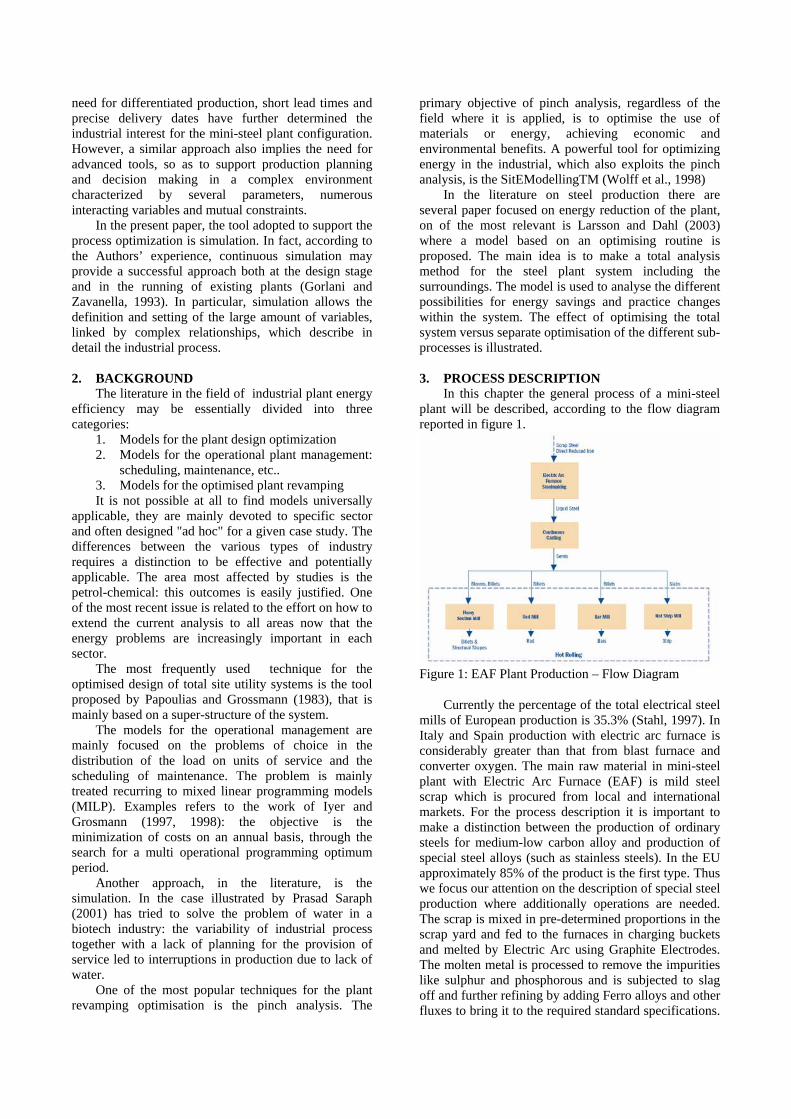
CC, LF’s, VD and EAF. Following we report the figures where we compare the real tap-to-tap times and simulated tap-to-tap times in the CC for a given representative casts set, used as reference for the validation. The figures show that the simulation is close to the real situation. In particular we calculate a mean error respect to the real data of 5.22%. The maximum distance between the simulated data and the real data is 7 min that represents the 15% of the real tap-to-tap CC time.

In the case of LFs we have compared the total simulated time with the total real time spent by the ladle in the LF station. This time takes into account the LF process time and the time spent waiting for the available

of the CC. Following we report the graph related to the LF validation. 

Figure 6: Validation of the CC time

 Figure 7: Validation of the LFs time

The mean error is 5.75%. Also in this case the

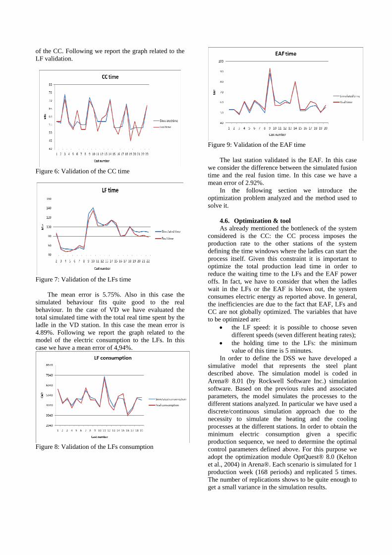
simulated behaviour fits quite good to the real behaviour. In the case of VD we have evaluated the total simulated time with the total real time spent by the ladle in the VD station. In this case the mean error is 4.89%. Following we report the graph related to the model of the electric consumption to the LFs. In this case we have a mean error of 4,94%.

 Figure 8: Validation of the LFs consumption

 Figure 9: Validation of the EAF time  

The last station validated is the EAF. In this case we consider the difference between the simulated fusion time and the real fusion time. In this case we have a mean error of 2.92%.

In the following section we introduce the optimization problem analyzed and the method used to solve it.

4.6. Optimization & tool As already mentioned the bottleneck of the system

considered is the CC: the CC process imposes the production rate to the other stations of the system defining the time windows where the ladles can start the process itself. Given this constraint it is important to optimize the total production lead time in order to reduce the waiting time to the LFs and the EAF power offs. In fact, we have to consider that when the ladles wait in the LFs or the EAF is blown out, the system consumes electric energy as reported above. In general, the inefficiencies are due to the fact that EAF, LFs and CC are not globally optimized. The variables that have to be optimized are:

• the LF speed: it is possible to choose seven different speeds (seven different heating rates);

• the holding time to the LFs: the minimum value of this time is 5 minutes.

In order to define the DSS we have developed a simulative model that represents the steel plant described above. The simulation model is coded in Arena® 8.01 (by Rockwell Software Inc.) simulation software. Based on the previous rules and associated parameters, the model simulates the processes to the different stations analyzed. In particular we have used a discrete/continuous simulation approach due to the necessity to simulate the heating and the cooling processes at the different stations. In order to obtain the minimum electric consumption given a specific production sequence, we need to determine the optimal control parameters defined above. For this purpose we adopt the optimization module OptQuest® 8.0 (Kelton et al., 2004) in Arena®. Each scenario is simulated for 1 production week (168 periods) and replicated 5 times. The number of replications shows to be quite enough to get a small variance in the simulation results.

4.7. Results In this section we report the results obtained via the

optimization of the simulative model described. In particular we show in figure 10 the electric energy consumption reduction obtained at the LFs.

 Figure 10: Comparison between the optimized electric consumption and the real electric consumption

 It is important to note that with the first 6 casts the

reduction of the electric consumption are not so significant because these casts have the VD process. In these cases the holding time is already reduced because the ladle has to go the VD for other operations. The only benefit of the optimization in the case of VD is the right choice of the LFs speed. Observing the results, we obtain a mean reduction of electric consumption of 21% at the LFs (18609 KWh). The adoption of this optimal strategy minimize the number of EAF power offs reducing the total time where the EAF is blown out (-21 min). This entails a reduction of the electric consumption of 14,700 KWh. 5. CONCLUSIONS

In the present work we have proposed a DSS that has the objective to set the speed and the holding time at the LFs in order to produce the sequence defined by the MRP system so as to reduce the electric energy consumption. Results obtained support company’s manager to optimize the usage of strategic leverage, since the DSS defines the solution taking into account the entire production process. In particular the overall electric energy saving is larger than 20%.

REFERENCES Cheung K.Y., Hui C.W., 2004. Total site scheduling for

better energy utilization, Journal of Cleaner Production, 12 (2), 171-184

Gorlani C. and Zavanella L., “Continuous simulation and industrial processes: electrode consumption in arc furnaces”, International Journal of Production Research, 1993, 31(8), 1873-1890

Iyer R.R., Grossmann I.E., 1997.Optimal multiperiod operational planning for utility systems, Computers and chemical engineering, 21, 787–800

Iyer R.R., Grossmann I.E., 1998. Synthesis and operational planning of utility systems for

multiperiod operation, Computers and chemical engineering, 22, 979-993

Kelton W.D., Sadowski R.P., Sturrock D.T., 2004. Simulation with Arena, McGraw Hill.

Larsson M. and Dahl J., 2003. Reduction of the Specific Energy Use in an Integrated Steel Plant—The Effect of an Optimisation Model, ISIJ International, 43 (10), 1664–1673

Papoulias, S. A., and Grossman, I. E., 1983. A structural optimization approach in process synthesis-I. Utility systems, Computers and chemical engineering, 7(6), 695-706.

Prasad V. Saraph, 2001. Simulating biotech manufacturing operations: issues and complexities. Proceedings of the 2001 Winter Simulation Conference, Arlington- VA (USA), 530-524.

Wolff A., Groebel M.J., Janowsky R., 1998. SitEModellingTM: a powerful tool for total site energy optimization, Computers and chemical engineering, 22, 1073-1084.

AUTHORS BIOGRAPHY IVAN FERRETTI, graduated in 2003 in Industrial Engineering at the University of Brescia (Italy). He took his Doctorate at the University of Brescia (Italy) in 2008. His main research interests are Simulation, Applied Meta-heuristics and Reverse Logistics. His e-mail address is : ivan.ferretti@ing.unibs.it.

SIMONE ZANONI, is currently an assistant professor in the Mechanical & Industrial Engineering Department at the University of Brescia (Italy). He graduated (with distinction) in 2001 in Mechanical Engineering and took his Doctorate at the University of Brescia (Italy) in 2005. His main research interests are: Layout Design, Inventory Management and Closed-loop Supply Chain. His e-mail address is : zanoni@ing.unibs.it.

LUCIO ZAVANELLA, is currently full professor in the Mechanical & Industrial Engineering Department at the University of Brescia (Italy). He graduated in 1982 in Mechanical Engineering at the Politecnico di Milano. Since 1986, he has been a researcher in the field of production systems at the Università degli Studi di Brescia. His research activities mainly concern manufacturing systems and inventory management, also with reference to environmental aspects. His e-mail address is: lucio.zavanella@ing.unibs.it.