evaluating the robustness of project performance under
TRANSCRIPT

Research on Economic Evaluation of Adaptation Measures to Climate Change under Uncertainty
Evaluating the Robustness of Project Performance under Deep Uncertainty of Climate Change: A Case Study of Irrigation Development in Kenya
Daiju Narita, Ichiro Sato, Daikichi Ogawada and Akiko Matsumura
No. 223
August 2021
JICA Ogata Sadako Research Institute
for Peace and Development
JICA Ogata Research Institute Working Paper
Use and dissemination of this working paper is encouraged; however, the JICA Ogata
Sadako Research Institute for Peace and Development requests due acknowledgement
and a copy of any publication for which this working paper has provided input. The views
expressed in this paper are those of the author(s) and do not necessarily represent the
official positions of either the JICA Ogata Sadako Research Institute for Peace and
Development or JICA.
JICA Ogata Sadako Research Institute for Peace and Development
10-5 Ichigaya Honmura-cho
Shinjuku-ku
Tokyo 162-8433 JAPAN
TEL: +81-3-3269-3374
FAX: +81-3-3269-2054

1
Evaluating the Robustness of Project Performance under Deep Uncertainty of
Climate Change: A Case Study of Irrigation Development in Kenya
Daiju Narita*†‡, Ichiro Sato§, Daikichi Ogawada** and Akiko Matsumura**
Abstract
While financing for climate adaptation projects is gaining prominence worldwide, the methods of performance evaluation of adaptation-related projects have not as yet been established. One reason for this is that future project effects are subject to deep uncertainty. As a case study of the evaluation of adaptation benefits under the uncertainty of climate change, we evaluate the robustness of the project performance of a Kenyan irrigation development project. Based on a simulation analysis carried out using the Robust Decision Making (RDM) approach, we assess the robustness of the positive expected outcomes of the project and find that the development of irrigation facilities, especially when combined with the soft adaptation measures of farming practices, could bring about an increase of household income in the future under a large variety of conditions. These beneficial effects are partly a reflection of the reduced damage from climate change achieved by the project. We conduct this study by utilizing the available resources and capacity of a development agency that has a scope of future applications to actual infrastructure projects. In this paper, we also discuss factors that could become relevant for the application of RDM-based project evaluation in the field of climate finance.
Keywords: climate change adaptation, climate finance, uncertainty, Robust Decision Making
(RDM), economic assessment, irrigation, agriculture, Africa
* Graduate School of Arts and Sciences, University of Tokyo, Tokyo, Japan ([email protected]) † JICA Ogata Sadako Research Institute for Peace and Development, Tokyo, Japan ‡ Kiel Institute for the World Economy, Kiel, Germany § Japan International Cooperation Agency (JICA), Tokyo, Japan ** Nippon Koei Co., Ltd, Tsukuba, Japan This paper has been prepared as part of a JICA Research Institute research project entitled “Economic Evaluation of Adaptation Measures to Climate Change under Uncertainty”. We benefited from discussions with and inputs by the following people: Ichiro Adachi, Kotaro Taniguchi, Hiroshi Takeuchi, Daigo Makihara, Yuji Masutomi, Kiyoshi Takahashi, Koji Dairaku, Wycliff Nyang’au, Martin Gomez-Garcia, Julie Rozenberg, Laura Bonzanigo, Stephane Hallegatte, and Marianne Fay. Seminar and meeting participants at the following venues and institutions provided us with valuable insights: JICA, JICA Research Institute, the National Institute for Environmental Studies, the JpGU Meeting 2018, the 2019 AGU Fall Meeting, and the Kenyan local stakeholders mentioned in the text.

2
1. Introduction
Climate change adaptation involves a large demand for infrastructure project finance, such as that
for irrigation, especially in developing countries. The UNEP Adaptation Finance Gap Report
(Puig et al. 2016) estimated that the costs of adaptation in developing countries could range from
US$140 billion to US$300 billion per year in 2030, and from US$280 billion to US$500 billion
per year in 2050. Infrastructure investment would account for a major part of this. Despite its
massive needs however, financial support for adaptation in developing countries falls far short of
expectation. Buchner et al. (2017) indicate that the average annual public climate finance 1
funding for adaptation in the years 2015 and 2016 was about US$22 billion, which partially
included funding in developed countries. The imbalance between mitigation and adaptation
finance has also provoked a lot of criticism. Less than 20% of public climate finance was spent
on adaptation in 2015/2016 (Buchner et al. 2017).
However, the amount of finance invested is not necessarily proportionate to the increase
in resilience to the negative impacts of climate change (climate resilience). Those projects that
can effectively enhance resilience need to be compared, identified, and given priority for funding.
Based on this recognition, a group of multilateral development banks (MDBs) and the
International Development Finance Club (IDFC) are developing a common framework for
“climate resilience metrics” (MDB and IDFC, 2019) to effectively assess, monitor and report the
contributions of their finance to the global goal of adaptation found in the Paris Agreement; that
is, “enhancing adaptive capacity, strengthening resilience and reducing vulnerability to climate
change” (Paris Agreement Article 7.1).
1 Public climate finance includes domestic and international finance by development finance institutions (DFIs) as well as international financial support to developing countries by donor governments/agencies and multilateral climate funds (Buchner et al. 2017). Note that it includes investments in developed countries by developed country DFIs.

3
In principle, project finance for climate change adaptation must be able to demonstrate
project effectiveness in the specified adaptations, but some challenges exist for establishing
evaluation methods in climate change adaptation projects. One of these challenges is the isolation
of climate benefits from the broad developmental benefits of projects when undertaking impact
evaluation. For example, the Green Climate Fund (GCF)2 recognizes that development projects
often have both “developmental and climate objectives,” but as a specialized climate fund, GCF
has set the principle that “those with purely developmental objectives should be financed from
sources other than GCF.” However, development and climate change benefits of projects are often
mixed and thus not easily isolated from each other3. For example, irrigation could both increase
current crop yields and mitigate yield losses in the future under climate change by ensuring and
regulating water input to farmlands, and these two effects cannot be qualitatively separated (a
detailed argument on the identification issue of adaptation effects is made by Lobell, 2014).
Given this difficulty, at the moment quantitative evaluation of the effectiveness of climate
change adaptation is not included in the practice of development finance. For example, the Japan
International Cooperation Agency uses a checklist approach where projects are regarded as
adaptation projects if certain qualitative criteria are met. Adaptation can be either the primary or
secondary objective of a project, and quantification of adaptation effects is not required to
establish eligibility to be called an adaptation project.
Another challenge for evaluation of climate change adaptation projects is that the effects
of climate change on human activities and well-being are uncertain. Often, local impacts of
climate change are unknown even in terms of their basic features – as discussed later in regard to
the precipitation trends at our case site in Kenya. But the presence of uncertainty does not mean
2 Green Climate Fund (2019), Review of the initial investment framework: Matters related to incremental and full cost calculation methodology and policies on co-financing and concessionality (GCF/B.23/19). 3 Jafino et al.’s (2021) global simulation analysis shows that the impacts of development policies and of climate change adaptation interventions are not always in agreement but sometimes oppose each other. The interrelationship between development intervention and climate risk vulnerability is also extensively discussed by Hallegatte et al. (2016, 2017, 2019).

4
that a project should be postponed. Because of the serious deficiency of knowledge, however,
conventional tools for project appraisal, such as cost-benefit analyses using expected net present
value, cannot simply be applied to the problem. In fact, in the context of developing countries,
substantial uncertainties are not limited to those of climate change effects. Future socioeconomic
conditions are likely to change greatly, and so are economic and demographic conditions, and
institutional and political structures.
In response to this paucity of information and the problem of what appraisal methods to
use in the practice of climate finance, we conduct a case study of a Kenyan irrigation development
project to demonstrate the evaluation of adaptation benefits under uncertainty of climate change
– a description of the project (the Mwea Irrigation Development Project) is given in Section 3.1.
This irrigation development project has a conventional objective as a development project to
improve the current agricultural productivity but also has benefits of staving off the negative
impacts of climate change on agriculture by guaranteeing water supply. We carry out analysis
based on the Robust Decision Making (RDM) approach, which highlights the vulnerabilities of a
project in the face of uncertainties – the conceptual basis of this approach is presented in the next
Section.
A distinctive feature of this study is that it was carried out based on the available
organizational capacity of a development agency with a scope for applying similar methods in
future project planning. Our simulation analysis shows that the irrigation development project
demonstrates generally positive results in terms of the robustness of performance relative to the
case without the project, and these positive effects are partly a reflection of the reduced damage
from climate change secured by the project, i.e., climate change adaptation. Meanwhile, our
results also highlight the importance of factors other than climate change as determinants of the
local economic conditions in the future. Indeed, the simulations show that the most influential
uncertainties affecting farmers’ average income level are demographic factors and the future
market prices of farm products, not climate change.

5
The rest of the paper is organized as follows. Section 2 provides an overview of the
conceptual foundations of our analysis, namely, the analytical frameworks of decision making
under uncertainty. Section 3 describes our case study, presents its results and their direct
implications in terms of project impact and climate change adaptation. Finally, Section 4 discusses
the general lessons obtained by the study for the future practical applications of RDM-based
project evaluation and summarizes the factors that could become relevant for uncertainty-
inclusive project evaluation in the practice of climate finance.
2. Conceptual and methodological frameworks
2.1. Risk and uncertainty in the context of project evaluation
Infrastructure development has a long- time horizon, and the levels of benefits are influenced by
unknown future factors such as the locality-specific impacts of climate change. Generally, its
impact evaluation needs to take account of limitations in existing knowledge of future conditions,
both internal and external to the project, during and after the construction. Depending on the
extent of lack of knowledge, analysts need to use different methods of project appraisal.
For some types of unknown futures (those involving “risk,” as defined by Knight 1921),
probabilistic distributions of potential outcomes are already well known – examples include
failures in engineering systems (such as those of aircraft and nuclear power plants) and the
occurrence of some types of natural disasters (earthquakes, etc.). Conventional risk analysis
approaches can be used for analysis of problems in this category. These methods include
probabilistic risk assessment in engineering, the Capital Asset Pricing Model in finance, and the
return period approach of river management, although the last example faces a serious challenge
from climate change. If the probability distributions of all possible futures are known, the cost-
benefit analysis of an infrastructure project is straightforward because it only needs to appraise

6
the expected net present value of the project derived from the probability-weighted sum of the net
present value for all future possibilities. The project is worth investing in if the expected net
present value is positive or above some cutoff value representing the opportunity cost.
Many other types of unknown futures, however, do not have known probability
distributions – these involve “uncertainty” as defined by Knight. The effects of climate change
on the costs and benefits of infrastructure fall in this category. For example, for Africa, even the
basic trends of local climatic patterns, such as whether precipitation will increase or decrease
under climate change, are predicted differently across the climate models used. In other words,
their reliable probability distributions do not exist.
The nature of uncertainties can be categorized into three types, namely, incomplete
knowledge, unpredictability, and disagreement (Sato and Altamirano, 2019). The level of
uncertainty varies depending on the extent of these three aspects, and their intense forms are called
deep uncertainty, which, as defined by Lempert (2003), arises when the experts do not know or
the parties to a decision cannot agree upon (i) the external context of the system, (ii) how the
system works and its boundaries, and/or (iii) the outcomes of interest from the system and/or their
relative importance. The effects of climate change are often characterized by deep uncertainty
(Walker et al. 2016).
Uncertainties could also be analyzed by using methods of risk analysis where objective
probabilities are replaced with subjective probabilities. Subjective probabilities are estimated by
the Bayesian inference that combines the analyst’s belief with observational (objective)
information on past events. In this approach, the expected net benefit of projects can be estimated,
and accordingly, cost-benefit analysis can be made.
For the problems involving uncertainties, however, the expected net benefit calculated
from the weighted sum of probabilistic future payoffs may not accurately reflect the real benefits
the decision makers may obtain from a project, unless it incorporates the possibilities that they
may adjust their future actions after the revelation of any truths that were previously uncertain.

7
For example, the expected net present value of preserving a forest does not reflect its real value
if the calculation does not take account of the fact that the forest could be converted to residential
areas anytime in the future when housing demand becomes high (the option value)4.
A complete method to analyze decision making under uncertainty with the possibility of
future adjustments of actions is stochastic dynamic optimization. Stochastic dynamic
optimization performs the analysis assuming that the risk-averse decision maker chooses actions
at every time point over a target time horizon in the face of future uncertainties. The objective of
these decisions is the maximization of time-discounted expected utility inclusive of the decision
maker’s risk preferences.
However, stochastic dynamic optimization is generally computationally demanding. A
more fundamental problem with the methods that use subjective probabilities is that these may
not be accurate, and so optimal solutions found by the analysis can also be wrong. Sometimes, a
small error in probability assessment leads to substantial differences in outcomes.
2.2. The Robust Decision Making (RDM) framework as a method of Decision Making
Under Deep Uncertainty (DMDU)
Given the above, for the analysis of decision making under uncertainty, the use of non-
probabilistic analytical approaches that do not compute the expected value but assess the
robustness of outcomes could be useful. Commonly used criteria for such non-probabilistic
uncertainty analyses are maximin (choosing an action whose worst possible outcome is least bad
among the available options), maximax (choosing an action whose best possible outcome is the
best among the available options), and minimax regret (choosing an action whose maximum
4 Real options analysis can incorporate such decision possibilities into evaluation, but as highlighted by Kwakkel (2020), its application to climate change adaptation involves some conceptual problems such as the inability to determine the expected value within each of individual scenarios over time by using the information of the expected value in an ensemble of concurrent scenarios.

8
regret is smallest and, where “regret” is defined as the deviation from the best outcome for each
contingency). A recent study that comprehensively examines and applies these alternative metrics
is McPhail et al. (2018). Methods that extend these frameworks with the orientations of practical
applications are DMDU (Decision Making Under Deep uncertainty) approaches (Marchau et al.
2019), which include the Robust Decision Making (RDM) method, dynamic adaptive pathways,
and the info-gap method. These methods do not analyze the optimality of decisions but the
robustness of decisions in the face of many future possibilities.
Among the DMDU methods, RDM analysis runs simulation models numerous times to
stress-test proposed decisions against a wide range of plausible futures (Lempert 2019). It does
not use probabilities and instead figures out how the system becomes vulnerable under possible
futures – it is an “agree-on-decisions” approach rather than an “agree-on-assumptions” approach.
RDM analysis is similar to conventional sensitivity analysis in the sense that it investigates system
behavior under changes of parameter levels. But unlike conventional “one-factor-at-a-
time“ sensitivity analysis, RDM examines simultaneous changes of multiple parameters rather
than the changes in individual parameters one by one, and also it seeks to find the conditions to
realize satisficing (positive or negative) outcomes for decisionmakers, rather than to quantify the
effects of input parameters on the outcomes (Sato and Altamirano 2019).
Lempert et al. (2019) show that an RDM analysis is generally composed of five steps,
namely: (1) Decision Framing; (2) Evaluate Strategy Across Futures; (3) Vulnerability Analysis;
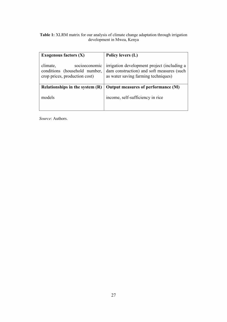
(4) Tradeoff Analysis; and (5) New Futures and Strategies. The Decision Framing step (1) utilizes
the XLRM framework, which considers the following four components: exogenous factors (X);
policy levers (L); relationships in the system (R); and output measures of performance (M). An
illustration of these elements is given in Section 3 based on the example of our case study. An
issue in the practices of decision making analysis is that because of limitations in analytical
capacity and in cognitive capacity for interpreting complex results, it is not possible to analyze
every conceivable uncertainty. It is therefore necessary to limit scenarios for analysis by focusing

9
on essential aspects for decision making, and for such scenario selections, the involvement of
stakeholders is needed. Following the Decision Framing step, an RDM analysis generates a large
number of scenarios where strategies are tested against those many possible scenarios that
represent uncertain futures (2), identifies how strategies are vulnerable under possible futures (3),
and evaluates tradeoffs among strategies (4). In the final step of an RDM analysis (5), analysts
and decisionmakers determine robust strategies in the face of uncertainties. But the results of this
fifth step can also be fed into the Decision Framing step again for another round of deliberations.
RDM originated from debates in the RAND Corporation over the better use of models in
situations where complex decisions had to be made in dynamic systems, and conventional
approaches were not useful (Lempert 2019). RDM began to be applied to public policy analysis
in the late 1990s (such as Lempert et al. 1996 and Rydell et al. 1997). In the field of international
development, the World Bank started experimenting with the RDM approach in decision analyses
for development projects such as flood management in Ho Chi Minh City, Vietnam (Lempert et
al. 2013), urban water supply in Lima Metropolitan Area, Peru (Kalra et al. 2015), and power and
water infrastructure development in several river basins in Africa (Cervigni et al. 2015). However,
the application of RDM in other development institutions is still scarce. The Inter-American
Development Bank helped Costa Rica develop a decarbonization plan using the RDM approach
and also demonstrated the applications of RDM to water and transport infrastructure planning
(Groves et al., 2020, 2021; Lempert et al., 2021).
3. Evaluation of future vulnerabilities under climate change: A case study of the Mwea
Irrigation Development Project
We conduct a case study as an application of the RDM method, not for project design but for
project evaluation. By using the RDM method, we evaluate the Mwea Irrigation Development
Project in Kenya in the presence of climate change effects in the future. The project aims to
10
develop irrigation infrastructure in the Mwea area of Kenya and increase crop production,
especially rice production, in that area. Through the analysis, we identify the vulnerabilities of
farmers’ income and local rice production to climate and other uncertainties. Robustness of
project outcome is assessed against two types of success criteria, namely, improvement in national
self-sufficiency of rice and the maintenance of farmers’ income levels.
Mwea (more precisely, the Mwea Irrigation Scheme; henceforth simply referred to as
Mwea) is the most important area of rice farming in Kenya, producing about 80% of rice in the
country (Atera et al., 2018). Rice is the third most important cereal crop in Kenya after maize and
wheat, and its consumption is growing. Most rice consumed in the country is imported, and in
response to this situation, the national government has set a long-term plan (the National Rice
Development Strategy: NRDS) to increase rice production and reduce import dependency
(Ministry of Agriculture, Livestock and Fisheries, 2014).
3.1. The Mwea Irrigation Development Project
The Mwea Irrigation Development Project is a project to build and rehabilitate irrigation
infrastructure (a dam and irrigation channels) in Mwea area of Kenya. It is conducted by the
Kenyan National Irrigation Board with a loan from the Japan International Cooperation Agency
(JICA). The area is located approximately 100 km northeast of Nairobi and is 1160 m above sea
level. The local climate is tropical with two rainy seasons, the long rainy season from March to
May and the short rainy season in October and November. Irrigation-related facilities have
gradually been developed since the 1950s in the area, and at present, local households
predominantly engage in farming, mainly rice cultivation, together with some horticulture.
Options for secondary income sources are limited in the area. The current irrigation development
project, which is ongoing as of January 2021, mainly deals with the construction of an irrigation
dam, whose location is outside the irrigated areas. See Narita et al. (2020) for more information.

11
Field-based geological, agronomic, and socioeconomic data were collected through
JICA’s assistance from feasibility study for the project, a JICA technical cooperation project in
Mwea (Rice MAPP project), and our original survey. The data include those about hydrology,
current cropping patterns, soil and other farming conditions, demographic and market conditions
in the region, and the institutional arrangements for water distribution.
The uncertainties from climate-related and socioeconomic parameters are considered in
the analysis. A list of uncertainties is shown in Appendix 1, and their specifications are discussed
in detail by Narita et al. (2020). We selected them in our assessment of the above-mentioned field
survey data together with discussions with local administrators and farmer representatives, which
took place in May 2017. Note that the simulations do not address any changes in the occurrence
of extreme weather events such as large-scale floods and prolonged droughts that might
potentially be induced by global climate change. Leaving out these extreme effects of climate
change partly reflects the limitations of our modeling capacity (as discussed in Narita et al. 2020),
but the non-extreme effects of climate change have their own importance and are thus worth
investigating – for example, a perceived general increase in temperatures, which is consistent
with the general trend of climate change, is among the concerns of local farmers.
Negative impacts of climate change could be reduced by changes in farming practices
and cropping patterns. We considered multiple options of cropping patterns and farming practices,
which had an emphasis on either rice or upland crops, and with the adoption of advanced farming
practices proposed and tested by the Rice MAPP project.
3.2. Simulations for scenario generation
We follow the steps of the RDM analysis method described in Section 2.2., although emphasis is
placed on scenario analysis (Steps 1-3) and not on the determination of favorable strategies
involving decisionmakers (Steps 4-5). For the Decision Framing, the XLRM matrix for our
12
analysis is shown in Table 1. The analysis involves simulations of economic outcomes that reflect
future climatic, hydrological and market conditions, and a full description of modeling details is
given in another paper, Narita et al. (2020). Our analysis considers various scenarios of climatic
and socioeconomic conditions (household number, crop prices, production cost) in the simulation
analysis (exogenous factors, X), where irrigation development projects and soft measures of
farming practices are taken into account as options for human intervention (policy levers, L). A
set of simulation models embodies the descriptions of relationships among variables
(relationships in the system, R) and evaluates incomes and the self-sufficiency of rice crops
(output measures of performance, M). For the Vulnerability Analysis, we employ methods of
scenario discovery, as described in the next subsection.
Income levels and rice production are estimated by using a combination of simulation
models for climate, hydrology, and crop yields. To be useful for scenario discovery analysis as
described below, a large number of simulations are made reflecting the uncertainties in key
parameters. The total number of simulation scenarios is approximately 24,000 (see also Appendix
1). Socioeconomic factors of the scenarios are generated by Latin Hypercube Sampling (LHS),
which is used to randomly select 100 sets of values differing in parameter levels. As for future
climate, hydrological, and socioeconomic conditions, we consider the years 2030 and 2050,
which are computed as the average over the periods 2021-2040 and 2041-2060.
Simulations are made by our model integrating outputs of the following existing models:
downscaled climate data from CMIP5 (Coupled Model Intercomparison Project Phase 5) climate
models and the WFEDI (WATCH-Forcing-Data-ERA-Interim) reanalysis weather data (climate)
(Weedon et al. 2014); the SHER model (hydrology) developed by Herath et al. (1990) and
previously applied in the Kenyan National Water Master Plan 2030 (2014); the DSSAT model
(yield) (Jones et al. 2003). For the downscaling of global circulation model (GCM) data to
estimate local climate conditions in Mwea, we used the delta change method utilized by
Prudomme et al. (2010) to extract the differences between the baseline and future climate

13
conditions from global climate models and add them to the baseline climate conditions based on
observational data (more precisely, reanalysis weather data, because observational data of local
weather conditions are limited in Mwea). Computed weather conditions are fed into a
hydrological model (SHER model), which is an empirical model incorporating the information
of local geology and simulates flows of local rivers as sources of irrigation water. Water
distribution within the target area is computed according to the simulated levels of river flows
and also to the existing arrangements for water allocations in the irrigation scheme, identified by
the previous field-based studies as mentioned above. Data of water availability and climate
conditions are used for yield estimations. For yield simulations, we use yield functions
approximating DSSAT to reproduce general conditions of agriculture in Mwea. Water input and
temperature are changed according to the simulated trends of climate change and are rendered
into yield gains or losses under climate change. A more complete description of our simulation
approach is given in Narita et al. (2020).
We performed two sets of simulation analyses in stages. First, we made a preliminary
analysis with a full set of model simulations and presented the results to government and local
stakeholders to collect their feedback. These meetings took place in May 2017 with
representatives of local agencies and organizations5 (the obtained information from the meetings
is summarized in Appendix 3). The main analysis is carried out using a revised simulation model
with adjustments of model structure and uncertainty formulations reflecting stakeholders’
concerns. This paper reports only on the results of the main analysis.
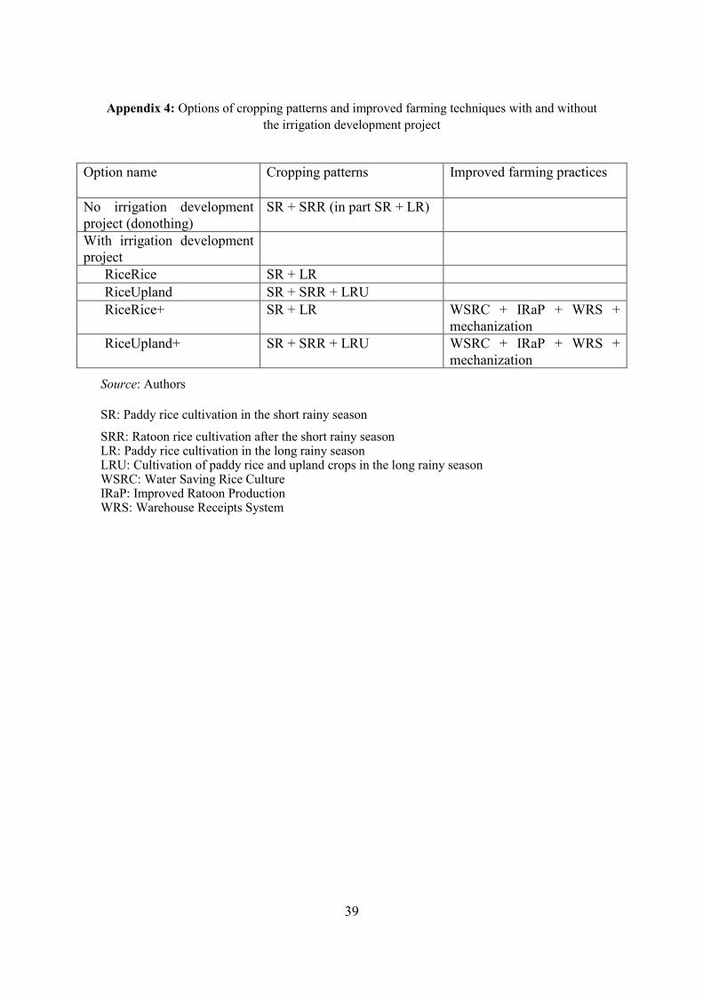
Simulations are conducted and organized for a no-project case (“donothing”) and four
cropping and project options, which are distinguished by whether the focus of farming is placed
on maximal rice production (“RiceRice”), or on diversification of crops combining the paddy rice
5 Namely, the following organizations: the Mwea Irrigation Agricultural Development Centre (MIAD), the National Irrigation Board (NIB), the Irrigation Water Users Association (IWUA), the Ministry of Water and Irrigation, the Ministry of Agriculture, Livestock and Fisheries, and the Kenya Meteorological Department.

14
cultivation and the upland farming of maize and vegetables (“RiceUpland”), and also by whether
additional non-irrigation means of improved farming are implemented or not (a “+” is given to
the option names for those with improved techniques, as in “RiceRice+” and “RiceUpland+”)
(see Appendix 4 and also Narita et al. 2020).
3.3. Method of scenario discovery
As a component of the RDM analysis, we perform scenario discovery analysis in the context of
the Mwea irrigation development scheme facing uncertain future climate change. Scenario
discovery aims to identify and display the key factors that best distinguish futures in which the
project meets its success criteria6. Through the May 2017 meetings with local stakeholders and
our own deliberation, we set two success criteria, namely, improvement in national self-
sufficiency of rice and maintenance of farmers’ income levels, whose household annual average
is approximately 300,000 KSh – in later analyses, the benchmark income level is set at this value.
The former, which is for improving Kenya’s food security and ameliorating its trade balance, is a
strong concern for the Kenyan government as stated in the NRDS. Our models do not simulate
Kenyan rice production at the country level but are based on the fact that Mwea accounts for most
of the Kenyan rice production. We make estimations of self-sufficiency by assuming the baseline
domestic rice production outside of Mwea is unchanged. For some of the results to be discussed
below, we estimate the values of total rice production in Mwea and evaluate them against the
benchmarks of the current production level (66,758 tons/year) and 100,000 tons/year.
Simulated income levels are examined to identify key vulnerabilities for the Mwea under
climate change. For scenario discovery, we utilize the Patient Rule Induction Method (PRIM:
discussed and applied by Groves and Lempert, 2007; Bryant and Lempert 2010; Matrosov et al.
6 Note that the word “scenario” used in the context of “scenario discovery” means a set of key system features (subspaces) to be identified by analysis, and that this usage is different from what the word means in the other parts of the paper, which are simply individual computational experiments.

15
2013; Kwakkel and Jaxa-Rozen, 2016). We employed the module of the PRIM for Python
developed and maintained by Jan Kwakkel and David Hadka (https://github.com/Project-
Platypus/PRIM), which is based on the Scenario Discovery Toolkit R package developed by the
RAND Corporation.
The PRIM is an algorithm that visualizes the future possibilities of a system as a set of
points in a high-dimensional space, where each dimension corresponds to an uncertain parameter.
The analysis seeks to find low-dimensional boxes in that space to cover more interested points
with higher density. In our case, these points are where the income level or rice production fails
the success criteria. Implicitly, a PRIM analysis is based on a functional relationship of variables
that could be represented as 𝑦𝑦 = 𝑓𝑓(𝑠𝑠, 𝐱𝐱) relating policy makers’ actions s to consequences of
interest y, conditional on a vector x representing a particular point in a multi-dimensional space
of uncertain model input parameters. By LHS, we construct a dataset of numerous combinations
of y and x, i.e., {𝑦𝑦𝑖𝑖 , 𝐱𝐱𝑖𝑖} (i=1,…,N). Given a cutoff level of policy success Yl, we can define the
set of interesting cases ls as 𝑙𝑙𝑠𝑠 = {𝐱𝐱𝑙𝑙�𝑓𝑓(𝑠𝑠, 𝐱𝐱) ≥ 𝑌𝑌𝑙𝑙}.
The size of boxes reflects a tradeoff of coverage and density and are defined as follows:
𝐶𝐶𝐶𝐶𝐶𝐶𝐶𝐶𝐶𝐶𝐶𝐶𝐶𝐶𝐶𝐶 = � 𝑦𝑦𝑖𝑖′
𝑥𝑥𝑖𝑖∈𝐵𝐵
� 𝑦𝑦𝑖𝑖′
𝑥𝑥𝑖𝑖∈𝑥𝑥𝑙𝑙�
𝐷𝐷𝐶𝐶𝐷𝐷𝑠𝑠𝐷𝐷𝐷𝐷𝑦𝑦 = � 𝑦𝑦𝑖𝑖′
𝑥𝑥𝑖𝑖∈𝐵𝐵
� 1𝑥𝑥𝑖𝑖∈𝐵𝐵
�
where B is the set of x in the chosen box, and also 𝑦𝑦𝑖𝑖′ = 1 if 𝐱𝐱𝑖𝑖 ∈ 𝑙𝑙𝑠𝑠 and 𝑦𝑦𝑖𝑖′ = 0
otherwise.
Large boxes can cover a large number of desirable points (i.e., the coverage is large),
while small boxes can encompass areas where there are relatively more interested points and less
uninterested points (i.e., the density is high). Normally, seeking high coverage results in low
density, and vice versa.

16
The analyst selects the most illustrative box for the purpose of analysis. Besides the
coverage and the density, the number of dimensions can also be selected, and this also involves a
tradeoff – a restriction in the number of dimensions brings about a clear and simple insight from
the analysis (i.e., interpretability is high), but is likely to reduce the coverage of the boxes.
3.4. The Modeling Results and Their Implications
Figure 1 is a plot of the simulation results of farmers’ average income for the reference years of
2030 and 2050. The graph takes the form of a violin plot, showing distributions of results where
the width of each shape represents the relative proportion of case occurrence at every value on
the vertical axis. The data show that the donothing option (no project) is generally worse than the
outcomes with the irrigation development project, and also, generally higher levels of income are
likely to be obtained through the use of improved farming techniques. The farmers’ income is
generally lower in 2050 than in 2030, and without both of the irrigation development project and
improved farming techniques, the income becomes lower than the baseline level for the majority
of scenarios in 2050.
Figure 2 shows similar results to those of Figure 1, except that they are outcomes under
a 1-in-10 year drought scenario. Income is generally reduced across the options relative to the
levels shown in Figure 1. Still, if both the irrigation project and a set of improved farming
techniques are in place, the majority of scenarios cross the benchmark level of 300,000 KSh/year,
regardless of the choice of rice-oriented farming (RiceRice+) or diversified crop farming
(RiceUpland+). These results suggest that the implementation of irrigation development, together
with the utilization of other improved farming techniques, could likely support farmers’
subsistence even under drought conditions in the future.
Figure 3 presents the results of simulating rice production. In the donothing option, many
scenarios exhibit significantly lower rice production than the baseline level of 2050, but such

17
possibilities of yield decrease are moderated in the options including the irrigation development
project. In fact, the negative shift of yield from 2030 to 2050 observed in the donothing case is
mostly blunted for the other four results. With the RiceRice+ option, the majority of scenarios
exceed rice production 100,000t/year. Meanwhile, no strong increase of rice production relative
to donothing is observed for the RiceUpland scenarios (those orienting towards crop
diversification without implementation of improved farming techniques), despite the increased
income as seen in the results presented in Figures 1 and 2. Based on the simulation results of rice
production in Mwea, we also made estimations of the self-sufficiency rate of rice in Kenya by
assuming the baseline domestic rice production outside of Mwea as unchanged. Results are
presented in Figure 4. A general tendency across the four project options is a transient
improvement in the rate in 2030 and a decrease in 2050, which is a reflection not only of yield
changes but also of changes in the demand for rice. In the long run, the self-sufficiency rate is
expected to worsen in most scenarios, and only intense rice farming under the RiceRice+ option
can generally exceed the present level of national rice self-sufficiency.
As a different representation of the results shown in the above Figures, Table 2
summarizes metric-based evaluations on the robustness of project performance regarding income
(Table 2a) and total rice production (Table 2b). It shows the mean, which would serve as the
ranking criterion of options under the principle of insufficient reason, the mean divided by the
standard deviation (the signal to noise ratio, SNR), which is utilized as a robustness metric in
existing studies such as Kwakkel et al. (2016), and Starr’s domain criterion (Starr 1963; Schneller
and Sphicas 1983), which in our case is defined as the proportion of the simulated cases which
satisfy the decision criteria given in the above (the average household income of 300,000 kSh/year
or the total rice production of 100,000 tons/year in the Mwea irrigation scheme). For the first two
indicators, both the absolute values and the ratios to those of the donothing option (values in
parentheses) are shown. The Table also presents the median, and the 10th and 90th percentiles. The
results show that for all the metrics considered, the options with the irrigation development project

18
exhibit a superior performance to the donothing option (without the irrigation development
project). Table 3 further extracts and tabulates the residuals of project benefits on income relative
to the donothing case – a graphical representation of this result is given in Appendix 5. It shows
estimates with and without the inclusion of climate change factors, the latter of which would
correspond to the “developmental benefits” mentioned in the Introduction. Despite a wide
spectrum of results across different project options, it generally shows that the project carries both
developmental and climate change-related benefits, while the latter becomes only significant in
2050 in some results.
The results of a PRIM analysis offer different insights on the potential project outcomes.
Figure 5 shows a density-coverage tradeoff plot (Graph a) and a box coverage plot (Graph b) for
the average household income in 2030 with the RiceUpland+ cropping option. The criterion for
evaluation is whether the average household can maintain the baseline level of average household
income (300,000 KSh/year). Graph (a) shows how the combinations of density and coverage of
interesting data points changes when the dimensions of parameters are restricted – note that as
mentioned in Section 3.3., density and coverage are in a relationship of tradeoff, as increasing
restrictions on the parameter space can enhance the proportion of interested points over the others
in the considered specific domain (i.e., higher density), but reduce the coverage of interested
points in the entire dataset (i.e., lower coverage). This plot helps us visualize the most influential
factors for the target system to fulfill the success criterion of average household income (i.e., the
annual level over 300,000 KSh). The colors of the circles represent differences in the number of
restricted dimensions. Dimensions are restricted in the sequence of: (i) the number of households
in Mwea; (ii) the market rice price; (iii) the cost of rice production; and (iv) the prices of upland
crops. Boxes with black outlines in Graph b are the areas covered by the Box corresponding to a
point on the trajectory of Graph a (Box 39, as indicated in the graph). The density-coverage
tradeoff plot suggests that the number of households in Mwea, the market rice price, and the cost
of rice production influence farmers’ income levels. The information of Graph b implies that

19
farmers’ income has a high likelihood of failure on the criteria when the number of households in
Mwea are greater than 15,000, the market rice price decreases by 9.38% or more, the total
production cost for Mwea is 1,600 million KSh or more, and the price increase of upland crops
are not very high (less than 8.15%).
Figure 6 shows results of a similar analysis to the above for rice production with the
RiceRice+ cropping option. The criterion here is whether the rice production in Mwea can achieve
the level of 100,000t/year. As an illustrative case, we choose Box 8 as indicated on the density-
coverage tradeoff plot (Graph a). Box 8 suggests that the criterion has a tendency to fail when the
temperature increase is over 1.33˚C, and the change in precipitation in the long and short rainy
seasons are within certain ranges (250.6mm and -157.1mm for LR and, 535.8mm and -49.8mm
for SR). It should be noted that demographic and price factors do not affect the rice production
outcomes because of the model structure we adopt.
Altogether, the results of Figures 5 and 6 imply that: (i) the physical amount of rice
production in Mwea, which has relevance for the national target, is influenced by climatic factors,
among which the clearest factor is the increase of the annual average temperature; and (ii) as for
the farmers’ income, the price factors (the market rice price and the production costs) and the
demographic factor of the Mwea community are more consequential than climate change.
4. Discussion and Conclusion
This study is a demonstration of the evaluation of a development project with the benefits of
climate change adaptation. The results show, among others, robust project benefits on household
income in the future under a large variety of climatic and socioeconomic conditions, especially
when combined with the soft adaptation measures of farming practices.
Unlike the widely practiced approach of using a qualitative checklist in appraisal of
climate change implications of development projects, we have attempted a quantitative estimation

20
of key socioeconomic outcomes with and without the project under climate change. A distinctive
feature of this study is that it was carried out based on the available organizational capacity of a
development agency with a scope for applying similar methods in future project planning. While
this assessment is not really tied to institutional decision making about financing infrastructure
construction, it offers some lessons for the practical application of this approach to the evaluation
of future projects.
In the context of climate change adaptation in developing countries, infrastructure
projects have two objectives; dealing with development and climate change. The former deals
with conventional development goals such as poverty reduction and economic growth, and this is
often more clearly appreciated than the latter. But a clear identification of the climate change
implications of a project is important since the climate change problem has the features of a global
public good (or global public bad), and hence the responsibility of the international community
as a whole is clear. Such an identification also allows us to directly associate climate finance with
climate benefits.
As a demonstration of the RDM method, our simulation results generally show a large
range of possible outcomes due to uncertainties. Our PRIM analysis also identifies the scenarios
where desirable levels of rice production and income are realized or not. This implies that for the
isolation of the project benefits involving the climate change objective from those of the
development objective, the consideration of uncertainty is fundamentally important.
To offer scope for potential future applications to other projects, our analysis is designed
to be as lean as possible in terms of the general data and modeling requirements. For example,
GCM and weather reanalysis data and the yield forecasting model are openly available, and
widely used yield forecasting and hydrological models are intentionally employed for analysis.
In this sense, in principle, a similar analysis could be made for many other irrigation development
projects throughout the world. It is worthwhile to note, however, that relative to general studies
of direct consequences of climate change, our study, focusing on knock-on effects of climate

21
change to local communities, necessitates a great amount of input of information about local
institutional arrangements and market conditions. For example, in the absence of any related data
for the future, our simulations simply assume the continuation of the existing regime of water
allocations and of the weak infrastructure that limits a prompt delivery of fresh produces, such as
tomatoes, to major markets. But changes in these factors can significantly alter the outcomes of
the analysis. In this way, our study is highly context specific.
We performed our analysis by utilizing the organizational framework and capacity of a
development agency, run in parallel to actual project implementation. Our experience hints that
the RDM method is potentially a useful and operational approach for the practical institutional
planning of development projects associated with climate change and other uncertainties. For
example, both the GCF and the Adaptation Fund, another international funding mechanism for
adaptation projects, emphasize that funding applications need to clarify their adaptation benefits
and stakeholder engagement in project development. RDM-based evaluations, which could
discern the adaptation and development benefits of projects, can be part of the application
documents for such schemes.
Another possibility for practical application, as highlighted by Bhave et al. (2016), shows
that there is some room for an RDM analysis to be associated with the process of Environmental
Impact Assessment (EIA), which is already mandatory for many public projects including
development projects. It is worth noting, however, that EIAs are not concerned with the
identification of project benefits, including those of climate change adaptation. Still, elements of
RDM analysis could be incorporated, for example, in the evaluation of negative climate-related
risks in an EIA process.
Thus, as seen from the perspective of the practices in development planning, RDM is not
a panacea, and certain issues and challenges exist for effective applications of the RDM approach.
This is in accordance with the arguments made by Bhave et al. (2016). First, an RDM analysis
for a climate change adaptation project is data intensive and necessitates expert knowledge of
22
multiple disciplines from climate science, hydrology, and engineering, to financial analysis. From
a practical standpoint, this necessity for a large amount of resources to be devoted to analysis may
mean that the evaluation is not best suited for screening of many projects potentially worthy for
financing but is rather for targeted applications to projects with large potential climate-related
impacts, such as large-scale infrastructure construction and land-use or urban development
planning.
Another challenge from a practical perspective of development assistance is how to
integrate RDM assessments into a well-established planning framework of conventional
infrastructure design and construction. Our assessment was performed externally to this. In the
communication with a broad range of institutions and people both in the donor and recipient
countries, such nuances and ambiguities are not easily conveyed. Also, in the context of
development projects, effectiveness of implementation greatly depends on the administrative and
coordination capacity of the recipient country. Since an RDM analysis on climate change
adaptation requires different types of data most likely scattered across different government
agencies, conducting an analysis can be difficult in countries where government ministries are
fragmented and not well coordinated.
As yet another aspect, our analysis has used two success criteria, one dealing with a
national goal (facilitation of self-sufficiency in rice production), and the other concerning needs
at the local level (farmers’ income), and in our case, the desirable outcomes according to these
two goals mostly coincide with each other. But the question remains as to how the focus of
evaluation should be set if the interests of local stakeholders and national-level-public officials,
or the interests of various groups of local stakeholders, differ. From a practical standpoint,
although RDM analysis is meant to facilitate public decision making when faced with uncertain
outcomes, it may not be effectively applied if the problems are deeply contentious.
Further, as communication with stakeholders in scenario development is an integral part
of an RDM analysis, challenges exist about effective communication with local stakeholders

23
regarding climate change. Local farmers face climate risks, such as heatwaves, and are likely not
to distinguish their current problem of risks and the future consequences of shifting trends.
Information easily becomes too complex to be digested, so it is desirable for consultations to take
place at multiple occasions. In the assessment, we consider the implications of climate change as
changes of general weather trends but not all kinds of future climate risks, such as floods. While
we attempted to communicate with stakeholders explicitly about the limitations of our analysis,
people often do not distinguish different types of climate risks, and a suitable analysis may be
viewed as the one incorporating all kinds of climate risks. In this sense, it might be useful to draw
on expert knowledge about the methods of risk communication in order to conduct an effective
RDM analysis in the context of climate change.
Nonetheless, stakeholder communication as a component of an RDM process could be
made as a constituent of the multi-level system of climate governance (Jänicke 2015, 2017;
Independent Group of Scientists appointed by the Secretary-General 2019). The usefulness of
stakeholder communication in the RDM processes could be associated with insights from the
scholarship on the public understanding of science. For example, Funtowicz and Ravetz (1993)
indicate that certain types of scientific inquiries, those of “post-normal science” by their definition,
necessitate a different approach to finding solutions from that of conventional (“normal”) science.
Project evaluation on climate change adaptation could be an issue of post-normal science as it
involves high system uncertainties and high “decision stakes,” which means that “all the various
costs, benefits, and value commitments that are involved in the issue through the various
stakeholders.” Funtowicz and Ravetz suggest that questions of post-normal science need to be
addressed by involving an “extended peer community,” which is made of all people with a stake
in the dialogue on the issue – people who participated in the process of RDM analysis could be
viewed as members of an extended peer community.

24
References
Atera, E. A., F. N. Onyancha, and E. O. Majiwa. 2018. “Production and marketing of rice in Kenya: Challenges and opportunities.” Journal of Development and Agricultural Economics 10 (3): 64-70.
Bhave, A. G., D. Conway, S. Dessai, and D. A. Stainforth. “2016. Barriers and opportunities for robust decision- making approaches to support climate change adaptation in the developing world.” Climate Risk Management 14: 1-10.
Bryant, B. P., and R. J. Lempert. 2010. “Thinking inside the box: A participatory, computer-assisted approach to scenario discovery.” Technological Forecasting and Social Change 77: 34-49.
Buchner, B., P. Oliver, X. Wang, C. Carswell, C. Meattle, and F. Mazza. 2017. Global Landscape of Climate Finance 2017. London: Climate Policy Initiative.
Cervigni, R., R. Loden, J. E. Neumann, and K. M. Srzepek, eds. 2015. Enhancing the climate resilience of Africa’s infrastructure. Washington DC: World Bank.
Funtowicz, S. O., and J. R. Ravetz. 1993. “Science for the post-normal age.” Futures 25(7): 739-55. Groves, D. G., and R. J. Lempert. 2007. “A new analytic method for finding policy-relevant
scenarios.” Global Environmental Change 17: 73-85. Groves, D. G., J. Syme, E. Molina-Perez, C. Calvo, L. Víctor-Gallardo, G. Godinez-Zamora, J.
Quirós-Tortós, F. De León, V.S. Gómez, and A. Vogt-Schilb. 2020. The Benefits and Costs of Decarbonizing Costa Rica’s Economy: Informing the Implementation of Costa Rica's National Decarbonization Plan under Uncertainty. Washington, DC: Inter-American Development Bank.
Groves, D. G., M. Miro, J. Syme, A. U. Becerra-Ornelas, E. Molina-Pérez, E. V. Saavedra, and A. Vogt-Schilb. 2021. Planificación de infraestructura hídrica para el futuro incierto en América Latina: un enfoque eficiente en costos y tiempo para tomar decisiones robustas de infraestructura, con un estudio de caso en Mendoza, Argentina. Documento de trabajo del BID 1162. Washington, DC: Inter-American Development Bank.
Hallegatte, S., M. Bangalore, L. Bonzanigo, M. Fay, T. Kane, U. Narloch, J. Rozenberg, D. Treguer, and A. Vogt-Schilb. 2016. Shock Waves: Managing the Impacts of Climate Change on Poverty. Climate Change and Development. Washington, DC: World Bank.
Hallegatte, S., A. Vogt-Schilb, M. Bangalore, and J. Rozenberg. 2017. Unbreakable: Building the Resilience of the Poor in the Face of Natural Disasters. Climate Change and Development. Washington, DC: World Bank.
Hallegatte, S., J. Rentschler, and J. Rozenberg. 2019. Lifelines: The Resilient Infrastructure Opportunity. Sustainable Infrastructure Series. Washington DC: World Bank.
Herath S., N. Hirose, and K. Musiake. 1990. “A computer package for the estimation of the infiltration capacities of shallow infiltration facilities.” In Proceedings of the 5th International Conference on Urban Storm Drainage, 111-18. Tokyo:
Independent Group of Scientists appointed by the Secretary-General, United Nation. 2019. Global Sustainable Development Report 2019: The Future is Now – Science for Achieving Sustainable Development. New York: United Nations.
Jänicke, M. 2015. “Horizontal and Vertical Reinforcement in Global Climate Governance.” Energies 8: 5782-99.
Jänicke, M. 2017. “The Multi-level System of Global Climate Governance – the Model and its Current State.” Environmental Policy and Governance 27: 108-21.

25
Kalra, N. R., D. G. Groves, L. Bonzanigo, E. M. Perez, C. Ramos, C. J. Brandon, and I. R. Cabanillas. 2015. Robust Decision-Making in the Water Sector: A Strategy for Implementing Lima’s Long-Term Water Resources Master Plan. Washington DC: World Bank.
Knight, F. H. 1921. Risk, Uncertainty and Profit. Boston and New York: Houghton Mifflin Company.
Kwakkel, J. H. and M. Jaxa-Rozen, 2016. "Improving scenario discovery for handling heterogeneous uncertainties and multinomial classified outcomes." Environmental Modelling & Software 79: 311-21.
Kwakkel J. H., S. Eker, and E. Pruyt. 2016. “How robust is a robust policy? Comparing alternative robustness metrics for robust decision-making.” In Robustness Analysis in Decision Aiding, Optimization, and Analytics. International Series in Operations Research & Management Science, edited by M. Doumpos, C. Zopounidis, and E. Grigoroudis, vol 241. Berlin: Springer.
Kwakkel, J. H. 2020. “Is Real Options Analysis fit for purpose in supporting climate adaptation planning and decision-making?” Wiley Interdisciplinary Reviews: Climate Change. doi:10.1002/wcc.638
Jafino, B. A., S. Hallegatte, and J. Rozenberg, 2021. “Focusing on differences across scenarios could lead to bad adaptation policy advice.” Nature Climate Change. https://doi.org/10.1038/s41558- 021-01030-9
Jones, J. W., G. Hoogenboom, C. H. Porter, K. J. Boote, W. D. Batchelor, L. A. Hunt, P. W. Wilkens, U. Singh, A. J. Gijsman, and J. T. Ritchie. 2003. “DSSAT Cropping System Model.” European Journal of Agronomy 18:235-65.
Lempert, R. J., 2019. “Robust Decision Making (RDM).” In Decision Making under Deep Uncertainty: From Theory to Practice, edited by V. A. W. J. Marchau et al. Berlin: Springer.
Lempert, R. J., M. E. Schlesinger, and S. C. Bankes. 1996. “When we don’t know the costs or the benefits: Adaptive strategies for abating climate change.” Climatic Change 33 (2), 235-74.
Lempert, R. J., S. W. Popper, and S. C. Bankes. 2003. Shaping the Next One Hundred Years: New Methods for Quantitative, Long-Term Analysis. Santa Monica, CA: RAND Corporation.
Lempert, R. J., and M. Collins, 2007. “Managing the risk of uncertain threshold responses: Comparison of robust, optimum, and precautionary approaches.” Risk Analysis 27 (4): 1009- 26.
Lempert, R., N. Kalra, S. Peyraud, Z. Mao, S. B. Tan, D. Cira, and A. Lotsch. 2013. Ensuring robust flood risk management in Ho Chi Minh City. Policy Research Working Paper No. 6456. Washington DC: World Bank.
Lempert, R.J., M. Miro, and D. Prosdocimi. 2021. A DMDU guidebook for transportation planning under a changing climate. IDB Technical Note 2114. Washington, DC: Inter-American Development Bank.
Lobell, D.B. 2014. “Climate change adaptation in crop production: Beware of illusions.” Global Food Security 3: 72-6.
MDB and IDFC. 2019. A Framework for Climate Resilience Metrics in Financing Operations: Consultation Draft. https://www.ebrd.com/documents/climate-finance/a-framework-for- climate-resilience-metrics-in-financing-operations.pdf?blobnocache=true
Matrosov, E. S., A. M. Woods, and J. L. Harou. 2013. “Robust decision making and info-gap decision theory for water resource system planning.” Journal of Hydrology 494: 43-58.
McInerney, D., R. Lempert, and K. Keller. 2012. “What are robust strategies in the face of uncertain climate threshold responses?” Climatic Change 112 (3–4): 547-68.

26
McPhail, C., H. R. Maier, J. H. Kwakkel, M. Giuliani, A. Castelletti, and S. Westra. 2018. “Robustness Metrics: How Are They Calculated, When Should They Be Used and Why Do They Give Different Results?” Earth’s Future 6: 169-91.
Ministry of Agriculture, Livestock and Fisheries. 2014. National Rice Development Strategy (2008- 2018), Revised Edition.
Narita, D., I. Sato, D. Ogawada, and A. Matsumura. 2020. “Integrating economic measures of adaptation effectiveness into climate change interventions: A case study of irrigation development in Mwea, Kenya.” PLoS ONE 15 (12): e0243779.
Puig, D., A. Olhoff, S. Bee, B. Dickson, and K. Alverson eds. 2016. The Adaptation Finance Gap Report. Nairobi, Kenya: United Nations Environment Programme.
Prudomme, C., R. L. Wilby, S. Crooks, A. L. Kay, and N. S. Reynard. 2010. “Scenario-neutral approach to climate change impacts: Application to flood risk.” Journal of Hydrology 390: 198-209.
Rydell, C. Peter., J. P. Caulkins, and Susan M. Sohler Everingham. 1997. Enforcement or treatment? Modeling the relative efficacy of alternatives for controlling cocaine. RP-614. Santa Monica, CA: RAND Corporation.
Sato, I., and J. C. Altamirano. 2019. Uncertainty, Scenario Analysis, and Long-Term Strategies: State of Play and a Way Forward. Working Paper. Washington, DC: World Resources Institute.
Schneller, G. O., and G. P. Sphicas. 1983. “Decision making under uncertainty: Starr’s domain criterion.” Theory and Decision 15 (4), 321-336.
Shortridge, J., S. Guikema, and B. Zaitchik. 2017. “Robust decision making in data scarce contexts: Addressing data and model limitations for infrastructure planning under transient climate change.” Climatic Change 140: 323-37.
Starr, M. K. 1963. Product Design and Decision Theory. New York: Prentice-Hall. UNEP. 2016. Adaptation Gap Report 2016. Copenhagen: UNEP-DTU Partnership. van Vuuren, D.P., J. Edmonds, M. Kainuma, et al. 2011. “The representative concentration
pathways: an overview.” Climatic Change 109: 5-31. Walker, W. E., R. J. Lempert, and J. H. Kwakkel. 2016. “Deep Uncertainty.” In Encyclopedia of
Operations Research and Management Science, edited by S. I. Gass and M. C. Fu, 395-402. New York: Springer.
27
Table 1: XLRM matrix for our analysis of climate change adaptation through irrigation development in Mwea, Kenya
Exogenous factors (X) climate, socioeconomic conditions (household number, crop prices, production cost)
Policy levers (L) irrigation development project (including a dam construction) and soft measures (such as water saving farming techniques)
Relationships in the system (R) models
Output measures of performance (M) income, self-sufficiency in rice
Source: Authors.

28
Table 2: Metric-based evaluations of project options The values in parentheses are the ratios to those of the donothing option. See Appendix 4 for specifications of the considered options. a. Average household income in Mwea (in thousand KSh per year)
RiceRice RiceUpland RiceRice+ RiceUpland+ donothing 2030 2050 2030 2050 2030 2050 2030 2050 2030 2050
Mean (principle of insufficient reason)
256 204 337 270 313 249 386 309 104 76 (2.5) (2.7) (3.2) (3.5) (3.0) (3.3) (3.7) (4.0)
Mean/STD (SNR)
6.7 3.9 6.9 3.9 7.3 4.0 7.4 4.0 5.1 3.2 (1.3) (1.2) (1.4) (1.2) (1.4) (1.2) (1.4) (1.2)
Starr’s domain criterion
0.15 0.05 0.73 0.33 0.57 0.23 0.97 0.49 0 0
Median 253 195 334 259 311 240 385 297 104 73 10th percentile 207 144 278 192 260 178 321 221 77 48 90th percentile 307 276 403 367 367 334 454 418 131 110
Source: Authors. b. Total rice production in Mwea (in thousand metric tons per year)
RiceRice RiceUpland RiceRice+ RiceUpland+ donothing 2030 2050 2030 2050 2030 2050 2030 2050 2030 2050
Mean (principle of insufficient reason)
82 82 70 69 101 100 86 86 67 64 (1.2) (1.3) (1.0) (1.1) (1.5) (1.6) (1.3) (1.3)
Mean/STD (SNR)
31.0 24.5 19.2 16.6 51.0 35.3 35.0 26.5 15.3 11.2 (2.0) (2.2) (1.3) (1.5) (3.3) (3.1) (2.3) (2.4)
Starr’s domain criterion
1 1 0.83 0.78 1 1 1 1 0.63 0.41
Median 83 82 71 70 101 101 87 86 69 65 10th percentile 79 78 64 62 99 98 85 84 60 56 90th percentile 85 85 72 72 103 103 88 88 71 70
Source: Authors.

29
Table 3: Relative benefits of project options These are estimated as the difference in annual average household income (in thousand KSh per household) from that of the no-project (“donothing”) option inclusive and exclusive of climate change-related effects (developmental and climate-related benefits of the project). See Appendix 4 for specifications of the considered options.
RiceRice+ RiceUpland+ 2030 2050 2030 2050
Without CC (develop-mental benefits)
With CC (develop-mental + climate-related benefits)
Without CC (develop-mental benefits)
With CC (develop-mental + climate-related benefits)
Without CC (develop-mental benefits)
With CC (develop-mental + climate-related benefits)
Without CC (develop-mental benefits)
With CC (develop-mental + climate-related benefits)
90th-percentile
240 249 222 235 322 335 297 317
Median 207 208 157 165 277 280 208 222 Mean 206 209 163 173 275 281 218 233 10th-percentile
173 170 116 122 230 231 158 165
Source: Authors.

30
Figure 1: Simulation results of farmers’ annual income for the year 2030 and year 2050 The violin plots represent the density distributions of case occurrence at each level of annual income, and the upper end, the middle line, and the lower end indicate the maximum, median and minimum. The baseline is the current level of the average annual income per household (in Kenyan Schillings, KSh). See Appendix 4 for specifications of the considered options.
Source: Authors.

31
Figure 2: Simulation results of farmers’ annual income in a 1-in-10 year drought The violin plots represent the density distributions of case occurrence at each level of annual income, and the upper end, the middle line, and the lower end indicate the maximum, median and minimum. The baseline, in which no drought is assumed, is the current level of the average annual income per household (in Kenyan Schillings, KSh). See Appendix 4 for specifications of the considered options.
Source: Authors.

32
Figure 3: Simulation results of rice production The violin plots represent the density distributions of case occurrence at each level of rice production, and the upper end, the middle line, and the lower end indicate the maximum, median and minimum. The baseline is the current level of annual rice production in the Mwea Irrigation Scheme (66,758 tons), and the graph also shows a reference line at 100,000 tons. See Appendix 4 for specifications of the considered options.
Source: Authors.

33
Figure 4: Simulation results of the self-sufficiency rate of rice in Kenya The violin plots represent the density distributions of case occurrence at each level of the national self-sufficiency rate for rice, and the upper end, the middle line, and the lower end indicate the maximum, median and minimum. The baseline is the current level of national rice sufficiency. See Appendix 4 for specifications of the considered options.
Source: Authors.

34
Figure 5: Results of a PRIM analysis for the average household income in 2050 with the RiceUpland+ cropping option
(a) Density vs. coverage tradeoff curve produced by the Scenario Discovery Toolkit. Colors represent differences in the number of restricted dimensions. Dimensions are restricted in the sequence of (i) the number of households in Mwea, (ii) the market rice price, (iii) the cost of rice production and (iv) the prices of upland crops. See also the text for interpretations of the graphs.
Source: Authors. (b) Box coverage plot for Box 39 indicated in the above Graph (a) (“# of households”: the number of households in Mwea; “rice price change [%]”: the market rice price; “total cost”: the cost of rice production; “crop price change [%]”: the prices of upland crops). The red points on the left graphs represent conditions where the success criteria were not met (the income is below the baseline level). Boxes with the black outline show the coverage of Box 39 in terms of the parameters considered.
Source: Authors.

35
Figure 6: Results of a PRIM analysis for the rice production in 2050 with the RiceRice+ cropping option
(a) Density vs. coverage tradeoff curve produced by the Scenario Discovery Toolkit. Colors represent differences in the number of restricted dimensions. Dimensions are restricted in the sequence of (i) change in the annual average temperature, (ii) precipitation in the long rainy season, and (iii) precipitation in the short rainy season.
Source: Authors. (b) Box coverage plot for Box 8 indicated in the above Graph (a) (“tas change [˚C]”: change in the annual average temperature; “pr change [mm/LR]”: precipitation in the long rainy season; “pr change [mm/SR]”: precipitation in the short rainy season). The red points on the left graphs represent conditions where the success criteria were not met (rice production in the Mwea is below 100,000 t/year). Boxes with the black outline show the coverage of Box 8 in terms of considered parameters.
Source: Authors.

36
Appendix
Appendix 1: Types and number of scenarios (uncertainties) considered in the analysis
Type of
uncertainty Number of scenarios Note
Climate scenarios
RCPs (CO2 concentration)
240 (4 x 60)
4 RCPs (RCP 2.6, RCP 4.5, RCP 6.0, RCP 8.5)
Climate conditions (temperature, precipitation)
60 combinations are selected by LHS from a range of values determined by outputs of 14 GCMs For the temperature increase from the baseline In 2030 Upper bound: 1.4˚C Lower bound: 0.6˚C In 2050 Upper bound: 2.4˚C Lower bound: 0.8˚C
(Baseline) 1 Socio-economic scenarios
Household number in Mwea
100 (LHS sampling)
In 2030 Upper bound: 47% increase Lower bound: no increase In 2050 Upper bound: 125% increase Lower bound: no increase
Price of rice See Appendix 2 for specifications Upper bound: no change Lower bound: 15% decrease
Price of upland crops
Upper bound: 10% increase Lower bound: 10% decrease
Production cost Upper bound: 30% increase Lower bound: 30% decrease
(Baseline) 1 Total (with CC) 24,000 Total (without CC) 100 Source: Authors.

37
Appendix 2: Estimated wholesale prices of crops
Commodity Unit Price (Ksh/kg)
Baseline* 2030**, 2050*** Rice (Basmati, short rain) 45 Upper bound: 45; lower bound:
38.5 Rice (Basmati, short rain ratoon)
33 Upper bound: 33; lower bound: 28.3
Rice (Basmati, long rain) 60 Upper bound: 60; lower bound: 51.4
Dry maize 41 41 Green gram 103 103 Tomato 78 78 Soybean 60 60 French bean 31 31
Source: Authors. * According to the Rice Mapp 2016 survey (Basmati), the Ministry of Agriculture, Livestock and Fisheries (dry maize, green gram, tomato), the SAPROF 2009 report (soybean, French bean); ** Growth rates set to be the same as those of the October 2017 World Bank Commodities Price Forecast; *** Set to be the same as the 2030 levels.

38
Appendix 3: Summary of information obtained from interviews in May 2017
We held meetings in May 2017 with the administrators of national agencies, staff at local
institutions and farmer representatives. These took the form of unstructured interviews in
combination with our presentation of data from our preliminary simulation analysis. Among
various concerns expressed by the participants, the household income of farmers and the national
goal of self-sufficiency of rice are most frequently mentioned as possible success criteria for
irrigation development.
Interviewees also noted that the following factors might affect the achievement of the desired
goals:
Supply of irrigation water and its allocation Water losses from the irrigation system Droughts due to decreased precipitation Illegal water harvest in the upstream areas Decline of the glaciers of Mount Kenya (river upstream) Decline of soil fertility due to continuous farming Crop damage by birds and other pests Fluctuations of market rice prices Fluctuations of farming costs, including the changes of government policy on
agricultural subsidies
Additionally, we also collected opinions about what measures besides irrigation development
could potentially raise or maintain crop yields under climate change
Introduction and diffusion of water-saving rice cultivation techniques Introduction and diffusion of improved crop varieties (varieties with high heat-,
drought- and disease-resistance) Improved management of cropping across the whole Mwea Irrigation Scheme Introduction and diffusion of farming of upland crops outside of the main cropping
seasons Repairs of irrigation channels to minimize water losses and the construction of water
reservoirs Tree planting in upstream areas
39
Appendix 4: Options of cropping patterns and improved farming techniques with and without the irrigation development project
Option name Cropping patterns Improved farming practices
No irrigation development project (donothing)
SR + SRR (in part SR + LR)
With irrigation development project
RiceRice SR + LR RiceUpland SR + SRR + LRU RiceRice+ SR + LR WSRC + IRaP + WRS +
mechanization RiceUpland+ SR + SRR + LRU WSRC + IRaP + WRS +
mechanization
Source: Authors
SR: Paddy rice cultivation in the short rainy season
SRR: Ratoon rice cultivation after the short rainy season LR: Paddy rice cultivation in the long rainy season LRU: Cultivation of paddy rice and upland crops in the long rainy season WSRC: Water Saving Rice Culture IRaP: Improved Ratoon Production WRS: Warehouse Receipts System

40
Appendix 5: Graphical representation of the relative benefits of project options as shown in Table 3 (“RR+”: RiceRice+; “RU+”: RiceUpland+). The ends and middle lines of the boxes
correspond to quartiles (i.e., the middle line represents the median), and the whiskers represent the furthest data points from the median within the 1.5 interquartile ranges (IQRs).
Source: Authors

Abstract (in Japanese)
気候変動に関する深い不確実性を考慮した事業効果の頑健性評価:
ケニアの灌漑開発 事業を対象としたケーススタディ
要約
世界的に気候変動適応事業への投資が増加する一方で、投資効果の評価手法は確立さ
れていない。その理由の一つとして、気候変動に対応する事業効果の評価には、深い不
確実性(deep uncertainty)が伴うためである。本研究では、ケニアの灌漑開発事業を
取り上げ、気候変動という不確実性下で計画される事業の効果を評価した。評価手法と
して、頑健(robust)な意思決定法(RDM)に基づくシミュレーション分析を行い、事業
により期待される効果の頑健性(robustness)評価を行ったところ、灌漑開発が将来起
こりうる様々な条件下において家計所得を増加させること、特に営農といった現場での
適応対策を合わせて実施する場合に顕著であることを明らかにした。これらの効果は、
事業実施を通じ実現した気候変動による被害の軽減を一部反映したものである。
なお、本研究の分析手法は、開発機関が実際の評価プロセスで実施可能な方法で行っ
ている。最後に本稿では,RDMに基づく事業評価を気候金融の分野に適用する際に関連
する様々な要素についても議論している。
キーワード: 気候変動適応、気候金融、不確実性、頑健な意思決定(RDM)、経済評価、
灌漑、農業、アフリカ
41

42
Working Papers from the same research project
Economic Evaluation of Adaptation Measures to Climate Change under Uncertainty
JICA-RI Working Paper No. 206 Integrative Economic Evaluation of an Infrastructure Project as a Measure for Climate
Change Adaptation: A Case Study of Irrigation Development in Kenya
Daiju Narita, Ichiro Sato, Daikichi Ogawada, and Akiko Matsumura