11/7/13

1

Features: representation, normalization, selection

Chapter 10

1

Features

v  Distinguish between instances (e.g. an image that you need to classify), and the features you create for an instance.

v  Features are “the workhorses of machine learning”: the quality of a classifier is crucially dependent on the features used to represent the domain.

v  Although many datasets come with pre-defined features, they can be manipulated in many ways

2

Features

v  Distinguish between instances (e.g. an image that you need to classify), and the features you create for an instance.

v  Features are “the workhorses of machine learning”: the quality of a classifier is crucially dependent on the features used to represent the domain.

v  Although many datasets come with pre-defined features, they can be manipulated in many ways: v  Normalization or other transformations v  Discretization v  Select the best features v  Combine features to compute new ones (feature construction)

3

Types of features

Quantitative (continuous) features: have a meaningful numerical scale   Examples: age, height etc.

Ordinal features: have an ordering   Example: house number

Categorical (discrete/nominal) features: not meaningful to describe them using mean, median v  Example: Boolean features

4

11/7/13

2

Features and classifiers

Some classifiers require numerical quantitative (linear classifiers). Need to transform an ordinal/categorical feature into a numerical feature. Assume we have a feature with possible values “lo”, “med”, “hi”. How would we transform this into one or more quantitative features? Note: SVMs and other kernel-based methods can be applied to ordinal/categorical data by way of an appropriate kernel function.

5

Features and classifiers

Some classifiers treat categorical and quantitative features differently. Examples: Naïve Bayes, decision trees Sometimes useful to use categorical features even if the underlying data is quantitative. Solution: discretization Aside: how about nearest neighbor classifiers?

6

Feature transformations

Aim: improve the utility of a feature by changing it in some way.

7

Feature transformations

Discretization: a mapping from a continuous domain to a discrete one. Thresholding: Simplest form of discretization that constructs Boolean features. How to choose the threshold? v  Unsupervised: mean/median v  Supervised: choosing the threshold to make the feature

most predictive (need a measure of how predictive a feature is)

8

11/7/13

3

Thresholding a feature

10. Features 10.2 Feature transformations

p.308 Figure 10.3: Thresholding

0 20 40 60 80 100 120 140 160 180 2000

5

10

15

20

0 20 40 60 80 100 120 140 160 1800

5

10

15

20

25

30

35

40

45

50

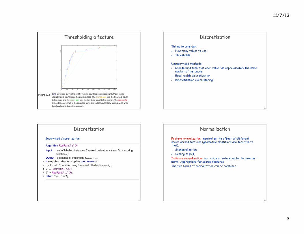
(left) Coverage curve obtained by ranking countries on decreasing GDP per capita,using 23 Euro countries as the positive class. The orange split sets the threshold equalto the mean and the green split sets the threshold equal to the median. The red pointsare on the convex hull of the coverage curve and indicate potentially optimal splits whenthe class label is taken into account. (right) Coverage curve of the same feature, using50 countries in the Americas as the positive class.

Peter Flach (University of Bristol) Machine Learning: Making Sense of Data August 25, 2012 309 / 349

9

10. Features 10.2 Feature transformations

p.308 Figure 10.3: Thresholding

0 20 40 60 80 100 120 140 160 180 2000

5

10

15

20

0 20 40 60 80 100 120 140 160 1800

5

10

15

20

25

30

35

40

45

50

(left) Coverage curve obtained by ranking countries on decreasing GDP per capita,using 23 Euro countries as the positive class. The orange split sets the threshold equalto the mean and the green split sets the threshold equal to the median. The red pointsare on the convex hull of the coverage curve and indicate potentially optimal splits whenthe class label is taken into account. (right) Coverage curve of the same feature, using50 countries in the Americas as the positive class.

Peter Flach (University of Bristol) Machine Learning: Making Sense of Data August 25, 2012 309 / 349

Figure 10.3

Discretization

Things to consider: v  How many values to use v  Thresholds. Unsupervised methods: v  Choose bins such that each value has approximately the same

number of instances v  Equal-width discretization v  Discretization via clustering

10

Discretization

Supervised discretization

11

10. Features 10.2 Feature transformations

p.311 Algorithm 10.1: Recursive partitioning

Algorithm RecPart(S, f ,Q)

Input : set of labelled instances S ranked on feature values f (x); scoringfunction Q.

Output : sequence of thresholds t1, . . . , tk°1.1 if stopping criterion applies then return ?;2 Split S into Sl and Sr using threshold t that optimises Q ;3 Tl = RecPart(Sl , f ,Q);4 Tr = RecPart(Sr , f ,Q);5 return Tl [ {t }[Tr ;

Peter Flach (University of Bristol) Machine Learning: Making Sense of Data August 25, 2012 313 / 349

Normalization

Feature normalization: neutralize the effect of different scales across features (geometric classifiers are sensitive to that). v  Standardization v  Scaling to [0,1] Instance normalization: normalize a feature vector to have unit norm. Appropriate for sparse features The two forms of normalization can be combined.

12

11/7/13

4

Logistic feature calibration

13

10. Features 10.2 Feature transformations

p.317 Figure 10.5: Logistic calibration of two features

0 1 2 3 4 5 6−1

0

1

2

3

4

5

6

7

−5 −4 −3 −2 −1 0 1 2 3 4 5

−5

−4

−3

−2

−1

0

1

2

3

4

5

0 0.1 0.2 0.3 0.4 0.5 0.6 0.7 0.8 0.9 10

0.1

0.2

0.3

0.4

0.5

0.6

0.7

0.8

0.9

1

(left) Two-class Gaussian data. The middle line is the decision boundary learned by thebasic linear classifier; the other two are parallel lines through the class means. (middle)Logistic calibration to log-odds space is a linear transformation; assuming unit standarddeviations, the basic linear classifier is now the fixed line F d

1 (x)+F d2 (x) = 0. (right)

Logistic calibration to probability space is a non-linear transformation that pushes dataaway from the decision boundary.

Peter Flach (University of Bristol) Machine Learning: Making Sense of Data August 25, 2012 320 / 349

10. Features 10.2 Feature transformations

p.317 Figure 10.5: Logistic calibration of two features

0 1 2 3 4 5 6−1

0

1

2

3

4

5

6

7

−5 −4 −3 −2 −1 0 1 2 3 4 5

−5

−4

−3

−2

−1

0

1

2

3

4

5

0 0.1 0.2 0.3 0.4 0.5 0.6 0.7 0.8 0.9 10

0.1

0.2

0.3

0.4

0.5

0.6

0.7

0.8

0.9

1

(left) Two-class Gaussian data. The middle line is the decision boundary learned by thebasic linear classifier; the other two are parallel lines through the class means. (middle)Logistic calibration to log-odds space is a linear transformation; assuming unit standarddeviations, the basic linear classifier is now the fixed line F d

1 (x)+F d2 (x) = 0. (right)

Logistic calibration to probability space is a non-linear transformation that pushes dataaway from the decision boundary.

Peter Flach (University of Bristol) Machine Learning: Making Sense of Data August 25, 2012 320 / 349

10. Features 10.2 Feature transformations

p.317 Figure 10.5: Logistic calibration of two features

0 1 2 3 4 5 6−1

0

1

2

3

4

5

6

7

−5 −4 −3 −2 −1 0 1 2 3 4 5

−5

−4

−3

−2

−1

0

1

2

3

4

5

0 0.1 0.2 0.3 0.4 0.5 0.6 0.7 0.8 0.9 10

0.1

0.2

0.3

0.4

0.5

0.6

0.7

0.8

0.9

1

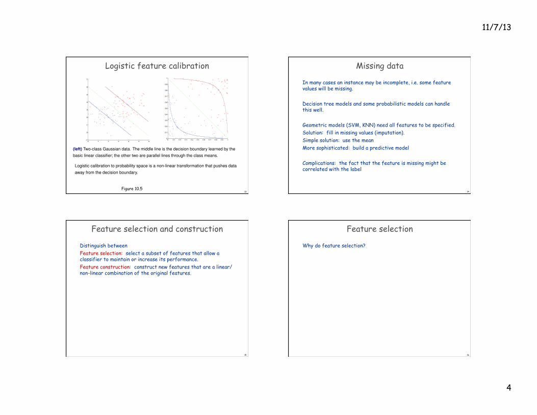
(left) Two-class Gaussian data. The middle line is the decision boundary learned by thebasic linear classifier; the other two are parallel lines through the class means. (middle)Logistic calibration to log-odds space is a linear transformation; assuming unit standarddeviations, the basic linear classifier is now the fixed line F d

1 (x)+F d2 (x) = 0. (right)

Logistic calibration to probability space is a non-linear transformation that pushes dataaway from the decision boundary.

Peter Flach (University of Bristol) Machine Learning: Making Sense of Data August 25, 2012 320 / 349

10. Features 10.2 Feature transformations

p.317 Figure 10.5: Logistic calibration of two features

0 1 2 3 4 5 6−1

0

1

2

3

4

5

6

7

−5 −4 −3 −2 −1 0 1 2 3 4 5

−5

−4

−3

−2

−1

0

1

2

3

4

5

0 0.1 0.2 0.3 0.4 0.5 0.6 0.7 0.8 0.9 10

0.1

0.2

0.3

0.4

0.5

0.6

0.7

0.8

0.9

1

(left) Two-class Gaussian data. The middle line is the decision boundary learned by thebasic linear classifier; the other two are parallel lines through the class means. (middle)Logistic calibration to log-odds space is a linear transformation; assuming unit standarddeviations, the basic linear classifier is now the fixed line F d

1 (x)+F d2 (x) = 0. (right)

Logistic calibration to probability space is a non-linear transformation that pushes dataaway from the decision boundary.

Peter Flach (University of Bristol) Machine Learning: Making Sense of Data August 25, 2012 320 / 349Figure 10.5

Missing data

In many cases an instance may be incomplete, i.e. some feature values will be missing. Decision tree models and some probabilistic models can handle this well. Geometric models (SVM, KNN) need all features to be specified. Solution: fill in missing values (imputation). Simple solution: use the mean More sophisticated: build a predictive model Complications: the fact that the feature is missing might be correlated with the label

14

Feature selection and construction

Distinguish between Feature selection: select a subset of features that allow a classifier to maintain or increase its performance. Feature construction: construct new features that are a linear/non-linear combination of the original features.

15

Feature selection

Why do feature selection?

16

11/7/13

5

Feature selection

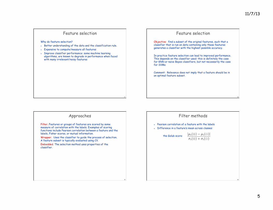
Why do feature selection? v  Better understanding of the data and the classification rule. v  Expensive to compute/measure all features v  Improve classifier performance: some machine learning

algorithms, are known to degrade in performance when faced with many irrelevant/noisy features

17

Feature selection

Objective: find a subset of the original features, such that a classifier that is run on data containing only these features generates a classifier with the highest possible accuracy. In practice feature selection can lead to improved performance. This depends on the classifier used: this is definitely the case for KNN or naive Bayes classifiers, but not necessarily the case for SVMs. Comment: Relevance does not imply that a feature should be in an optimal feature subset.

18

Approaches

Filter. Features or groups of features are scored by some measure of correlation with the labels. Examples of scoring functions include Pearson correlation between a feature and the labels, Fisher scores, or mutual information. Wrapper. Uses the classifier to guide the process of selection. A feature subset is typically evaluated using CV. Embedded. The selection method uses properties of the classifier.

19

Filter methods

v  Pearson correlation of a feature with the labels v  Difference in a feature’s mean across classes:

the Golub score:

20

|µi(�)� µi( )|�i(�) + �i( )

11/7/13

6

How many features?

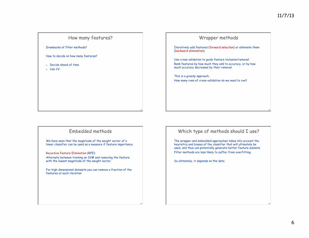
Drawbacks of filter methods? How to decide on how many features? v  Decide ahead of time. v  Use CV.

21

Wrapper methods

Iteratively add features (forward selection) or eliminate them (backward elimination) Use cross validation to guide feature inclusion/removal: Rank features by how much they add to accuracy, or by how much accuracy decreases by their removal. This is a greedy approach. How many runs of cross-validation do we need to run?

22

Embedded methods

We have seen that the magnitude of the weight vector of a linear classifier can be used as a measure if feature importance. Recursive Feature Elimination (RFE): Alternate between training an SVM and removing the feature with the lowest magnitude of the weight vector. For high dimensional datasets you can remove a fraction of the features at each iteration

23

Which type of methods should I use?

The wrapper and embedded approaches takes into account the heuristics and biases of the classifier that will ultimately be used, and thus can potentially generate better feature subsets. Filter methods are less likely to suffer from overfitting. So ultimately, it depends on the data.

24

11/7/13

7

Bias in feature selection

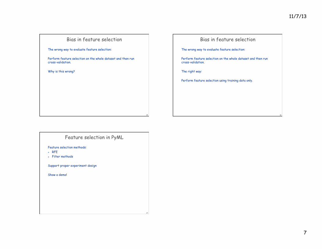
The wrong way to evaluate feature selection: Perform feature selection on the whole dataset and then run cross-validation. Why is this wrong?

25

Bias in feature selection

The wrong way to evaluate feature selection: Perform feature selection on the whole dataset and then run cross-validation. The right way: Perform feature selection using training data only.

26

Feature selection in PyML

Feature selection methods: v  RFE v  Filter methods

Support proper experiment design Show a demo!

27