fluro scence
TRANSCRIPT

7/28/2019 Fluro Scence
http://slidepdf.com/reader/full/fluro-scence 1/15
Journal of Pharmaceutical and Biomedical Analysis
22 (2000) 325–339
Analysis of film coating thickness and surface area of pharmaceutical pellets using fluorescence microscopy and
image analysis
Martin Andersson a, Bjorn Holmquist b, Jorgen Lindquist c, Olle Nilsson a,Karl-Gustav Wahlund a,*
a Department of Technical Analytical Chemistry, Centre for Chemistry and Chemical Engineering , Lund Uni 6ersity, P.O. Box 124 ,
S -221 00 Lund , Swedenb Department of Mathematical Statistics, Lund Uni 6ersity, P.O. Box 118 , S -221 00 Lund , Sweden
c Analytical Chemistry, Pharmaceutical R&D, AstraZeneca R&D Molndal , S -431 83 Molndal , Sweden
Received 24 June 1999; received in revised form 1 October 1999; accepted 14 November 1999
Abstract
A method is presented which enables geometrical characterisation of pharmaceutical pellets and their film coating.
It provides a high level of details on the single pellet level. Image analysis was used to determine the coating thickness
(h) applied on the pellets and the surface area (A) of the pellet cores. Different definitions of A and h are evaluated.Hierarchical analysis of variance was used to resolve different sources contributing to the total variance. The variance
within pellets and the variance between pellets were found as significant sources of variation. Special emphasis was
put on evaluation of A/h due to its influence on the release rate of an active drug substance from the pellet core. The
pellet images were thus used to predict variations in the release rate using a mathematical model as a link between
the image data and the release rate. General aspects of image analysis are discussed. The method would be useful in
calibration of near infrared spectra to h in process analytical chemistry. © 2000 Elsevier Science B.V. All rights
reserved.
Keywords: Image analysis; Pellets; Coating; Thickness; Surface area; Hierarchical analysis of variance; Release rate
www.elsevier.com/locate/ jpba
1. Introduction
There is a need to characterise products manu-
factured within the pharmaceutical industry.
These products are usually obtained in a series of
operations, one of which is the film coating pro-
cess. The film coating is applied using a fluidised
bed process [1], where pellet cores of 0.1–1 mm in
diameter containing the active drug are covered
with a permeable membrane, a coating layer. By
this, the dissolution after administration of the
drug is prolonged, and controlled release can be
* Corresponding author. Tel.: +46-46-2228316; fax: +46-
46-2224525.
E -mail address: [email protected] (K.-G.
Wahlund)
0731-7085/00/$ - see front matter © 2000 Elsevier Science B.V. All rights reserved.
PII: S 0 7 3 1 - 7 0 8 5 ( 9 9 ) 0 0 2 8 9 - 7

7/28/2019 Fluro Scence
http://slidepdf.com/reader/full/fluro-scence 2/15
M . Andersson et al . / J . Pharm. Biomed . Anal . 22 (2000) 325–339 326
obtained. The release rate of the active drug is
influenced by many factors. Important ones are
the thickness of the coating applied (h) and the
surface area (A) of the pellets [1]. The release rate
is high for pellets having thin h and large A, and
low for pellets with thicker h and smaller A [1].
Thus, the characterisation of the product in terms
of A and h can serve to optimise the process in
which the coated pellets are produced.
The mass of the coating applied can be used as
an indirect measure of h and A. It can thus be
used to predict the release rate [2] of the active
drug. Another indirect method, based on assum-
ing perfect spheres and using experimentally de-
termined densities and mass measurements of the
coating for a sample of pellets, can be used to
reveal both the average h and average A of the
pellets [3]. Moreover, the release rate as a function
of the specific area can be obtained indirectly
from sieve analysis [4–7].
Image analysis [8,9] could enable a direct mea-
surement of h but has so far been concerned
mostly with particle size and roundness parame-
ters [1,10–13]. These are determined from images
obtained by scanning electron microscopy or cam-
eras facilitated with magnification using, e.g. a
visible light microscope, all in order to study the
influence of the geometrical parameters upon the
release rate. Kanerva et al. [14,15] compared the
results from image analysis and laser light diffrac-
tion methods to the results obtained from sieve
analysis for both spherical particles and differ-
ently shaped particles. Image analysis was con-
cluded to be the optimal method for narrow size
distributions. The two methods gave similar re-
sults and enabled the size distribution of pellets to
be determined. With image analysis, pellet shape
parameters could also be studied.
For direct determination of h on pharmaceuti-
cals, only a few examples have been presented sofar. Moussa et al. [16–18] studied the increase in
gel thickness of tablets in water at 37°C using a
light transmission image analysis system. After
given time intervals, the tablet was removed and
frozen in liquid nitrogen, sliced along its axial
direction and the increase in gel thickness could
be studied along the radial direction. Wesdyk et
al. [19,20] studied h on pellets sliced into two
sections. The pellets were photographed using a
scanning electron microscope, the average film
thickness was determined, however only from
three measurements, and its influence on the re-
lease rate was evaluated. It should be noted that
the image analysis technique is of general charac-
ter and can be found in a wide area of applica-
tions, e.g. material technology [21– 26] medical
science [27–31], and membrane science [32,33], to
mention a few.
The objective of this study was to develop
image analysis methods for determination of h
and A. The latter can be used to predict variations
in the release rate using its dependence on varia-
tions in A/h. In addition, methods for studying
individual segments of the pellet core surface and
their association with the corresponding h were
developed. To the best of our knowledge no such
work has yet been presented. The study was per-
formed on a large number of pellets (394) and a
large number of thickness measurements within
each pellet (100), enabling statistical analysis of
the results. The method described can provide
with information on specific sources of variation
such as the homogeneity within pellets and be-
tween pellets within a batch. Notably, h as well as
A can be defined in many different ways, espe-
cially in the case of non-ideal geometry, here
non-perfect spheres. Details on this was another
important aim for the study while in previous
studies the definitions were often not given, but
instead the image analysis system and its software
were referred to. A further objective was to de-
velop a method that would be suitable for cali-
brating near infrared spectra to h. This would be
used for in-line process analytical chemistry of the
coating process [34].
2. Experimental
2 .1. Materials
Pellet cores containing the active drug sub-
stance were manufactured in-house and sieved to
a diameter of ca. 400– 500 mm. The shape was
approximately spherical with a ratio of maximum
to minimum radius in the range of 1.1– 1.8 for

7/28/2019 Fluro Scence
http://slidepdf.com/reader/full/fluro-scence 3/15
M . Andersson et al . / J . Pharm. Biomed . Anal . 22 (2000) 325–339 327
95% of the pellets. The coating material was ethyl
cellulose applied as a solution in ethanol. For
each batch experiment :10 kg of pellet cores was
used in which dry air (B10% RH) was used for
fluidising the pellet bed. Different manufacturing
conditions were considered where each experiment
was performed in a pilot-scale process equipment.
Samples were taken from each batch at :75, 100
and 125% of the empirical target amount of coat-
ing solution added. Each batch was thus run
longer than needed, putting the real target
amount of coating in the centre of the study.
2 .2 . Sample preparation
From each sample taken out from a batch, 12
pellets were examined utilising a method similar
to that presented by Wesdyk et al. [19]. Each
pellet was glued onto a black anodised 15×15×
1 mm iron plate. The glue was smeared out to a
thin layer to ensure that only the bottom of the
pellet was fixed to the glue. The pellets were
bisected using an in-house constructed equipment
with a vertical rotating axis and a table with
variable height position. Each iron plate, with its
attached pellet, was placed on a horizontal mag-
netic disc fixed on top of the rotating axis. With
the axis rotating, the iron plate was slid on the
magnet until the pellet was in the centre of rota-
tion. The height position of the table was adjusted
to ensure that the pellet would be cut in its
equator. This was accomplished by performing
the cutting underneath a stereo light microscope,
and consequently the height position of the cut-
ting blade could be comprehended and the cutting
was performed in the midplane. During rotation
at :10 s per revolution, each pellet was carefully
cut by manually pushing a Microtome blade into
the pellet. The blade was slid on the table, making
the cutting operation steady and stable, and it wasnoted that the shape of the pellets were not af-
fected by the cutting. This procedure was repeated
for 33 samples, totalling 33×12=396 pellets.
2 .3 . Image examination
After being cut, each pellet was photographed
using a camera coupled to an incident light
fluorescence microscope (Fig. 1A). This took ad-
vantage of the fact that the core and the coating
showed fluorescence but with different intensities.
The colour images were stored on a Kodak Photo
CD and converted to bitmap files, readable for
the Matlab Image Processing Toolbox. With a
macro routine, the inner and outer borders of the
coating were marked at 20– 30 points using the
computer mouse, to define the respective borders
(Fig. 1B). At places were the borders were chang-
ing in a more curved manner, the points were
chosen closer to each other, to capture the overall
curvature. The points of the inner and outer
border, respectively, were connected using an in-
terpolating parametric cubic spline curve, imple-
mented in Matlab Spline Toolbox (Fig. 1C). The
two borders were stored as vectors, containing
:2000 points, respectively. The inner border was
split into segments of the perimeter defined by
equidistant points along it. For each of these
segments the corresponding thickness were mea-
sured. Thus, a thickness vector for each pellet,
consisting of 100 elements was obtained. The
thickness of each pellet could hence be regarded
as a population of thickness rather than a single
thickness value (Fig. 1D). All distances in the
images were converted to micrometers using a
scaling factor. This scaling factor was obtained
with the accuracy of the 1-mm ruler used, which
can be considered very good. The precision in the
conversion factor was determined to be :0.07%
in relative S.D. A total of 100 points positioned at
equal distances along the curve representing the
inner border were chosen and different definitions
of thickness and area were used. From the already
examined pellets, eleven of these were randomly
chosen to be studied again after 6 months to get
an estimate of the repeatability of the method.
2 .4 . Definitions of coating thickness
Three different definitions of h were evaluated.
One of them was based on the minimum distances
from the inner border to the outer border. The
second definition was based on the distances from
the inner border to the outer border, forced to be
locally perpendicular to the inner border. In the
third definition, the distances between the bor-

7/28/2019 Fluro Scence
http://slidepdf.com/reader/full/fluro-scence 4/15
M . Andersson et al . / J . Pharm. Biomed . Anal . 22 (2000) 325–339 328
Fig. 1. Fluorescence microscopy image of a coated pellet (A), cut in two halves. The brighter section shows the thin film coating on
the core (dark inner section) that contains the active drug substance. The manually marked points (B) are connected using an
interpolating parametric cubic spline curve (C). One hundred individual measures of h (D) reflect the distribution of h. Here the
minimum distances from the inner border to the outer border are shown.
ders, required to be an extension of the radii
originating from the centre of gravity of the pellet,
were used.
2 .5 . Definitions of pellet core segment surfacearea
Three different models for determination of Ai
of the pellet core segments shown in Fig. 2 were
defined. The cutting plane of the pellets is here
referred to as the equatorial plane and accord-
ingly, the poles of the pellet will be found perpen-
dicular to the equatorial plane.
Fig. 2. Ai of a pellet core. The measured segment width in the
cutting plane, w, is shown together with the measured equato-
rial radius, ri ,e, and the estimated radius to the poles, ri , p.

7/28/2019 Fluro Scence
http://slidepdf.com/reader/full/fluro-scence 5/15
M . Andersson et al . / J . Pharm. Biomed . Anal . 22 (2000) 325–339 329
Fig. 3. Illustration of the different models for A. (A) Surface
area model 1. All segment areas are of equal size (black
sections) based on the average equatorial radius. (B) Surface
area model 2 with differently sized segments based on only the
equatorial radius for that segment. (C) Surface area model 3
using ellipsoids to describe each of the segments. See Section
2.5 for details.
sliced out from an ellipsoid where w is estimated
as a fraction (1/100) of the pellet core perimeter.
The segment surface area is then
Ai =
w:r i ,e2 +
ri ,er i ,p2 arccosh
ri ,e
ri ,p
r i ,e2 −r i ,p
2 ;, ri ,e\ri ,p
wr i ,e2 , ri ,e=ri ,p
w
:r i ,e2 +
ri ,er i ,p2 arcsin
r i ,p2 −r i ,e
2
ri ,p
r i ,p
2 −r i ,e2
;, ri ,eBri ,p
(3)
where ri ,e and ri ,p denote the principal semi-axes
of the ellipsoid, based on a circular equator
with the radius ri ,e. Hence, two of the semi-axes will be equal to ri ,e for the ellipsoid which
is used to obtain Ai of that pellet core seg-
ment. The polar radius was defined as ri ,p=1
100 100 j =1 r j ,e and used for all of the segments within
a pellet.
In general, all of the segments will coincide in
the poles and Ai of the segments within a pellet
will not be equally large (Fig. 3C).
2 .6 . Ratio of pellet core surface area to coating
thickness
By using the definitions of h and Ai , each
individual Ai can be associated with its corre-
sponding thickness measurement, hi to determine
Ai /hi for individual segments. In order to limit the
study of individual Ai /hi , the three different mod-
els for Ai were used, but for hi , the minimum
distance was used only.
2 .7 . Hierarchical analysis of 6
ariances
The variances of h on pellets and A/h were
examined using hierarchical analysis of variance
[35], to enable evaluation of different types of
variances, at different levels of detail. Hierarchical
analysis of variance can be performed when the
structure of the data is nested which was the case
here. The analysis is based on the fact that the
2 .5 .1. Surface area model 1
This model was based on assuming that eachpellet core could be described by a perfect sphere
(Fig. 3A). All the 100 segments around the pellet
were assumed to be equally large, 1/100 of total A
of the pellet core
Ai =1
1004yr core2 (1)
The pellet core average radius was determined as
the mean of all the individual segment radii in the
equatorial plane, r core=1
100 100 j =1 r j ,e.
2 .5 .2 . Surface area model 2 In the second model, the segments of the pellet
core are assumed to be sliced out from perfect
spheres of different sizes (Fig. 3B). In each of the
100 segments, Ai is assumed to be 1/100 of a
sphere with the radius ri ,e,
Ai =1
1004yr i ,e2 (2)
Consequently, each individual pellet core segment
is assumed to have the same polar radius
as equatorial radius, i.e. ri ,p
=ri ,e
for each in-
dividual segment (Fig. 2). In general, the
area segments within a pellet will not be equally
large, and the segments will not coincide in the
poles.
2 .5 .3 . Surface area model 3
A more rigorous model is one where Ai is
approximated by a segment with the width, w,
Â Ã Ã Ã Ã Ì Ã Ã Ã
à Å
7/28/2019 Fluro Scence
http://slidepdf.com/reader/full/fluro-scence 6/15
M . Andersson et al . / J . Pharm. Biomed . Anal . 22 (2000) 325–339 330
total variance can be written as a sum of several
variances,
| total2 =|1
2+|22+|3
2+|42+|5
2 (4)
where | i 2 denote statistically independent vari-
ances. These are determined from experimental
variances obtained as deviations around the mean
value at the level i , | i ,exp2 . The individual variances
were |12=variance between batches, estimated
from |21,exp−|
22,exp, |
22=variance between sam-
ples taken at 75, 100 and 125% of the target
processing time (within any batch), estimated
from |22,exp−|
23,exp, |3
2=variance between pellets
(within any sample, within any batch), estimated
from |23,exp−|
24,exp, |2
4, variance between different
positions around the pellet (within any pellet,
within any sample,…), estimated from |24,exp−
|2
5,exp
, and |2
5
=variance between replicate mea-
surements (within any position around the pellet,
within any pellet,…)=|25,exp. The individual vari-
ances were calculated in a step-wise procedure.
The deviation around the average of replicate
measurements would give |25=|
25,exp, and further
on, the deviation of measurements at different
places around their mean would give |24,exp. The
estimation of |24 could then be obtained from the
subtraction, |24,exp−|
25,exp. The remaining statisti-
cally independent variances were obtained
accordingly.
The hierarchical analysis of variance, i.e. the
estimation of the statistically independent |21
through |25, was numerically performed using
Matlab. Standard statistical packages do not usu-
ally contain routines for hierarchical analysis of
variance when the data set is unbalanced and very
large, as was the case here.
3. Results and discussion
The results obtained from image analysis were
used to characterise h on the pellets. They also
provided possibilities to predict the influence of
the geometrical parameters on the release rate.
This was enabled by a hierarchical analysis of
variance which also gave a detailed description of
the variations in the pellets such as variation
within pellets and variation between pellets.
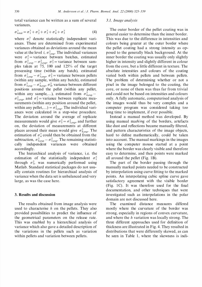
3 .1. Image analysis
The outer border of the pellet coating was in
general easier to determine than the inner border.
This was due to the difference in intensities and
colours being greater at the outer border where
the pellet coating had a strong intensity as op-
posed to the generally black background. At the
inner border the coating was usually only slightly
higher in intensity and slightly different in colour
from the core, but a little different in texture. The
absolute intensities and colours of the coating
varied both within pellets and between pellets.
The problem of determining whether or not a
pixel in the image belonged to the coating, the
core, or none of them was thus far from trivial
and could not be based on intensities and colours
only. A fully automatic, computerised analysis of
the images would thus be very complex and a
computer program was considered taking too
long time to implement, if ever possible.
Instead a manual method was developed. By
using manual marking of the borders, artefacts
like dust and reflections became manually filtered,
and pattern characteristics of the image objects,
hard to define mathematically, could be taken
into account. The manual markings in the images
using the computer mouse started at a point
where the border was clearly visible and therefore
easy to determine, and then points were marked
all around the pellet (Fig. 1B).
The part of the border passing through the
manually marked points needed to be constructed
by interpolation using curve fitting to the marked
points. An interpolating cubic spline curve gave
satisfactory agreement with the visible border
(Fig. 1C). It was therefore used for the final
documentation, and other techniques that were
investigated such as interpolations in the polar
domain are not discussed here.The examined distance measures differed
mostly where the curvature of the border was
strong, especially in regions of convex curvature,
and where the h variation was locally strong. The
three different approaches used for definition of
thickness are illustrated in Fig. 4. They resulted in
distributions that were differently skewed, as can
be seen in Table 1, where the skewness is indi-

7/28/2019 Fluro Scence
http://slidepdf.com/reader/full/fluro-scence 7/15
M . Andersson et al . / J . Pharm. Biomed . Anal . 22 (2000) 325–339 331
cated by the large deviations from the average to
the maximum thickness. The most useful defini-
tion of the thickness would be the minimum dis-
tance from a point at the inner border to a point
at the outer border because the diffusion rate is
here maximal and thus dominates the release rate.
The definition of Ai , based on the param-
eters shown in Fig. 2, was also found to be
non-trivial, because it could be based on a
population of radii, the mean radius, or the
mean of the surface associated to each of the
radii. The area measures were more sensitive to
the choice of definition than the thickness mea-
surements were. This can be seen when data in
Fig. 4. The different definitions of h. Minimum distance (A), locally perpendicular (B), and extension of the radius from the centre
of gravity (C). The sub-images are from the upper right corner of the images of Fig. 1.
Table 1
Comparison of h obtained from the different thickness definitionsa
Thickness (h)995% C.I./mmDefinition
Average (N =89)Minimum (N =1) Maximum (N =1)
8094 44.690.6Minimum distance 2194
96942194 45.190.6Locally perpendicular
46.290.685942194Radius extension
a 100% coating applied.

7/28/2019 Fluro Scence
http://slidepdf.com/reader/full/fluro-scence 8/15
M . Andersson et al . / J . Pharm. Biomed . Anal . 22 (2000) 325–339 332
Table 2
Comparison of A of the pellet core obtained from different segment surface area models
A995% C.I./(103 mm2)Individual segment surface area, Ai 995% C.I./(103 mm2)Segment surface area model
Maximuma (N =1) Total sum (N =389)Minimuma (N =1)
10.990.11 718.490.54.390.1
16.990.2 688.090.52 1.490.211.190.14.290.1 701.290.53
a Individual segments.
Table 2 are compared with data in Table 1. An
important factor in this comparison is that calcu-
lations of A include square terms of the individual
radii in the equatorial plane.
3 .2 . Hierarchical analysis of 6ariance
For an ideal homogeneous manufacturing of
perfectly spherical pellets with equal sizes and a
measurement method for h with no error or ran-
dom variation, all variance would be found in |22,
i.e. the variance between samples taken out at
different processing times (Eq. (4)). There would
be no variance between batches, between pellets,
between measurements nor between replicate
measurements. The reason for the non-zero vari-
ance of |22 is, of course, that it covers the system-
atic change in thickness during manufacturing.
Obviously, as demonstrated in Fig. 1, the ideal
situation is not existing and hierarchical analysis
of variance was performed in order to quantitate
the different variances contributing to the total
variance. The total variance was split into the
separate components mentioned above, but some
confounding still remained, e.g. the variation
caused by not cutting exactly in the equator of the
pellet. This variation would be a part of |23 using
this hierarchical model. Still, it should be noted
that it is not sure that optimal release propertiescome with ideal, homogeneous geometry.
The different thickness variances obtained from
Eq. (4) were calculated and their estimates are
presented in Table 3. The 95% confidence limits
were also calculated. During calculation, the dis-
tributions were evaluated using normal-plots,
showing the distributions around the averages at
the different levels. The distributions of the h
appeared to be close to normally distributed, Fig.
6, except for some of the extreme values. Since the
individual values of |i were estimated from differ-
ences between the experimentally obtained |i ,exp,
it is obvious that |1 is small. |1,exp and |2,exp
appear as practically identical. However, due to
the few replicates at that level, the confidenceinterval becomes large.
A closer examination of the normal plots re-
veals that the thickness distributions are slightly
asymmetrical (Fig. 5) and have a slight skewness
towards large values compared to what would be
expected if they were normally distributed. Since
|22 is dependent on the process time interval, it
would be of interest to see if it is dependent on the
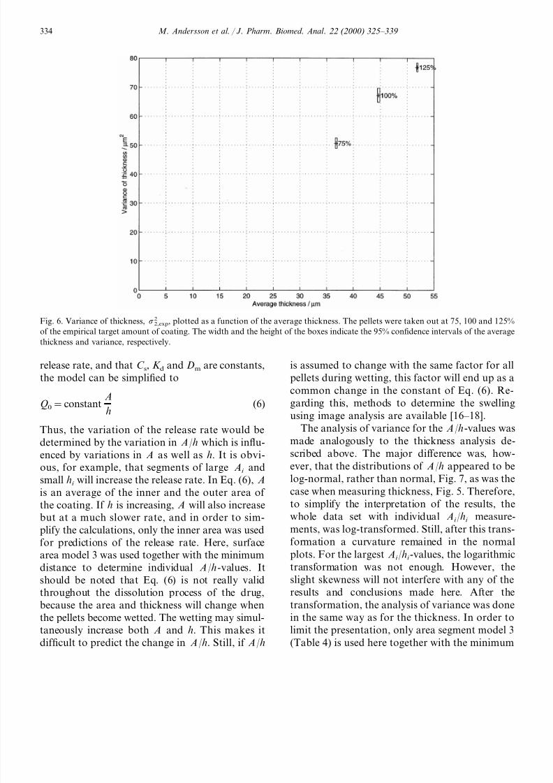
thickness. And, indeed, the plot in Fig. 6 shows
that |22,exp increases with the average h for sam-
ples taken out at different processing times corre-sponding to 75, 100 and 125% of the empirical
target amount. This is in close agreement with
what was obtained by Wnukowski et al. for a
similar type of process [36]. It means that if,
instead, the hierarchical analysis was based on
thickness-corrected variances, |2i /hi , the |2
2/h con-
tribution would become less important. This may
be corrected for by using a square root transfor-
mation of the individual thickness values [37].
Here, however, the range of thickness for different
Table 3
Standard deviation of thicknessa
|1/mm |2/mm |4/mm |5/mm|3/mm
7.9 5.45.1 3.8
[3.7–4.1][4.8–5.9][0–7.9] [4.6–5.6][2.5–12.0]
a Numbers within brackets are the 95% confidence intervals.

7/28/2019 Fluro Scence
http://slidepdf.com/reader/full/fluro-scence 9/15
M . Andersson et al . / J . Pharm. Biomed . Anal . 22 (2000) 325–339 333
Fig. 5. Deviations of minimum h around average values. Traces 1–5 represent the levels in the hierarchical model. Residual=0
denotes the average value for each level. From these deviations, |i ,exp were determined, see text for details.
degrees of coating is rather restricted, see Fig. 6,
and the effect of such transformation would hence
be quite limited. Still, without any thickness cor-
rection, the obtained |22 will represent some aver-
age of variation depending on the process timeinterval. This average will closely represent |2
2 at
the 100% degree of coating.
The repeatability in the marking of the border
was tested for by repeating the marking of the
inner and outer borders in eleven of the already
examined images after six months. Of course, the
curves defining the inner and outer borders, be-
came slightly different. These differences were
mostly due to difficulties in determining the bor-
ders of the diffuse parts, at some parts resulting in
a border inside, and at other parts resulting in a
border outside the border first drawn, in a ran-
dom manner. This repeatability is found in the
hierarchical structure and is denoted |25.
The precision of the conversion factor from
pixel-units to micrometers was determined from
repeated measurements using a 1-mm ruler. This
suggested that the variance caused by imprecision
in the scaling factor was negligible, and therefore
it was not taken into account for further analysis.
However, it would be possible to extend the hi-
erarchical model with another level.
3 .3 . Predicted influence on the release rate
Since the pellets studied are intended for con-
trolled release formulations, their variation in re-
lease rate was evaluated from their geometrical
properties. The release rate is depending on A/h,
usually included as a proportionality factor re-
gardless of the order of the model. A simple
model, assuming zero-order release rate may be
described by
Q0=A
hC sK dDm (5)
where Q0 is the zero-order release rate, C s is the
solubility of the drug substance, K d is the parti-
tion coefficient of the drug substance to the coat-
ing and Dm is the diffusion coefficient of the drug
substance in the coating. Assuming zero order
7/28/2019 Fluro Scence
http://slidepdf.com/reader/full/fluro-scence 10/15
M . Andersson et al . / J . Pharm. Biomed . Anal . 22 (2000) 325–339 334
Fig. 6. Variance of thickness, |22,exp, plotted as a function of the average thickness. The pellets were taken out at 75, 100 and 125%
of the empirical target amount of coating. The width and the height of the boxes indicate the 95% confidence intervals of the average
thickness and variance, respectively.
release rate, and that C s, K d and Dm are constants,
the model can be simplified to
Q0=constantA
h(6)
Thus, the variation of the release rate would be
determined by the variation in A/h which is influ-
enced by variations in A as well as h. It is obvi-
ous, for example, that segments of large Ai and
small hi will increase the release rate. In Eq. (6), A
is an average of the inner and the outer area of
the coating. If h is increasing, A will also increase
but at a much slower rate, and in order to sim-
plify the calculations, only the inner area was used
for predictions of the release rate. Here, surface
area model 3 was used together with the minimum
distance to determine individual A/h-values. It
should be noted that Eq. (6) is not really valid
throughout the dissolution process of the drug,
because the area and thickness will change when
the pellets become wetted. The wetting may simul-
taneously increase both A and h. This makes it
difficult to predict the change in A/h. Still, if A/h
is assumed to change with the same factor for all
pellets during wetting, this factor will end up as a
common change in the constant of Eq. (6). Re-
garding this, methods to determine the swelling
using image analysis are available [16–18].The analysis of variance for the A/h-values was
made analogously to the thickness analysis de-
scribed above. The major difference was, how-
ever, that the distributions of A/h appeared to be
log-normal, rather than normal, Fig. 7, as was the
case when measuring thickness, Fig. 5. Therefore,
to simplify the interpretation of the results, the
whole data set with individual Ai /hi measure-
ments, was log-transformed. Still, after this trans-
formation a curvature remained in the normal
plots. For the largest Ai /hi -values, the logarithmic
transformation was not enough. However, the
slight skewness will not interfere with any of the
results and conclusions made here. After the
transformation, the analysis of variance was done
in the same way as for the thickness. In order to
limit the presentation, only area segment model 3
(Table 4) is used here together with the minimum

7/28/2019 Fluro Scence
http://slidepdf.com/reader/full/fluro-scence 11/15
M . Andersson et al . / J . Pharm. Biomed . Anal . 22 (2000) 325–339 335
Fig. 7. Deviations of the log (Ai/hi) around their average values. Traces 1– 5 represent the levels in the hierarchical model.
Residual=0 denotes the average value for all levels. From these deviations, |i ,exp were determined.
Table 4
Comparison of log (Ai/hi) obtained from different segment Ai definitions using the minimum thickness as hia
log (A/hmin)995% C.I.Segment surface area model
Maximumb (N =1)Minimumb (N =1) Meanb
(N =89)
1 5.990.14.390.1 5.0690.01
6.190.23.990.2 5.0090.012
3 4.790.1 5.490.1 5.0590.01
a 100% coating applied.b Individual segments.
Table 5
Standard deviation of log (A/h)a
|2|1 |3 |4 |5
0.20 0.13 0.0960.18
[0.18–0.21] [0.12–0.14] [0.091–0.101][0.04–0.3][0–0.25]
a Numbers within brackets are the 95% confidence intervals.

7/28/2019 Fluro Scence
http://slidepdf.com/reader/full/fluro-scence 12/15
M . Andersson et al . / J . Pharm. Biomed . Anal . 22 (2000) 325–339 336
thickness. In Table 4 it can be seen that indepen-
dently of the definition chosen, they end up with
quite similar results for the average values. The
results from the hierarchical analysis of variance
of log (Ai /hi ) are presented in Table 5. From these
results, one can conclude that a significant source
of variation in the data came from variation
between the pellets, |23, and also within the pellets,
|24. The inhomogeneity of the raw material in
terms of non-ideal geometry, was thus found as a
significant source of variation. The hierarchical
analysis of variance of log (Ai /hi ) gave very simi-
lar results for all of the area models studied,
except for model 2. Thus, for levels l, 2, 3 and 5,
in Eq. (4), any of the models can be used, but at
level 4 (variance within pellets) the choice of
model has a significant role. The variance at level
4 was significantly smaller for the area models l
and 3. To find out which model is the most
accurate, further experiments are needed, e.g. by
slicing the pellets in more than two sections and
using methods from stereology.
For all models, the variance between pellets
(level 3) were practically the same, ranging from
|3=0.19 to 0.20. The variance, |2CR, that is con-
nected to an average of log (A/h)pellet of any sam-
ple examined for controlled release profiles can be
estimated from the variance of log (A/h) between
pellets, |23, divided by the number of pellets, n, in
the sample,
|CR2 =|3
2
n(7)
This is because the observed release rate of a
sample is depending on the sum of n individual
log (A/h)pellet contributions having the variance
|23. Hence, the mean release rate in a sample of n
pellets has the variance |23/n.
Since the log-transformed data were close to
normally distributed and the data set was very
large, about 95% of the expected variation of
log (A/h) for any sample containing n pellets,
would be covered by the interval
log (A/h)=v392' |3
2
n(8)
where v3 represents the expectation value of
log (A/h) at level 3. Eq. (8) could also be applied
Fig. 8. Predicted confidence intervals for the relative release rate as a function of the number pellets. The upper and lower limits were
obtained using Eq. (10).

7/28/2019 Fluro Scence
http://slidepdf.com/reader/full/fluro-scence 13/15
M . Andersson et al . / J . Pharm. Biomed . Anal . 22 (2000) 325–339 337
Fig. 9. Simulation of release rate for 50 trials with one pellet (A) and 50 trials with 100 pellets (B). The simulated curves were
obtained using Eq. (10) and normally distributed random numbers.

7/28/2019 Fluro Scence
http://slidepdf.com/reader/full/fluro-scence 14/15
M . Andersson et al . / J . Pharm. Biomed . Anal . 22 (2000) 325–339 338
to this investigation, but to get a relevant picture
of how the variances were affecting the release
rate, the results were inversely transformed, using
the exponential function. To reflect the variation
of the release rate around the mean value for
different numbers of pellets, an interval with a
confidence level of 95% would be
A/h=ev39
2|3
n=ev39
0.40
n (9)
and this interval is obviously non-symmetric. As
an alternative to this, the release rate, constant
A/h, may be related to the average release rate to
obtain a relative release rate (A/h)rel by dividing
Eq. (9) with ev3, yielding
A
h rel=
ev39
2|3
n
ev3=e
92|3
n=e9
0.40
n (10)
Eq. (10) could be plotted for different n which is
shown in Fig. 8. It is obvious that the variation
diminished rapidly as the number of pellets was
increased. The variation becomes more symmetric
for large values of n. The interval is below 92%
for n]400, and even smaller for the number of
pellets, :103, used in a relevant dose for the
material studied here.
As an alternative, the variation of different
release rates could be illustrated when employing
simulations for different number of pellets, using
Eq. (10) and normally distributed random num-
bers for |3. Such simulations are shown in Fig.
9A and B, drawn in the same scaling using arbi-
trary units, and it is obvious that geometrical
variations influence variations in the release rate.
Of course, when real dissolution tests are per-
formed, a larger variance can be expected due to
further sources of variation, such as non-ideal
zero-order dissolution, variations in coating den-
sity, coating porosity, and when considering dif-ferent types of coating. In addition, variations are
introduced in the dissolution experiments.
4. Conclusions
The image analysis method can be used to
reveal details and characteristics of the material
such as variations of h within pellets and between
pellets. The quality of the pellets can be deter-
mined at different levels of detail using hierarchi-
cal analysis of variance. In addition, the image
analysis data can be used to predict the variations
in release rate due to geometrical variations in the
pellets.
The method presented can further be used as a
reference method for calibrating near infrared
reflectance spectra to h, which can then be used as
a quick and non-destructive in-line process analyt-
ical chemical method for determination of h [34].
Knowledge of both the average h, and its variance
are then very helpful parameters in order to cali-
brate and to characterise these measurements.
Acknowledgements
Mats O. Johansson, AstraZeneca R&D Moln-
dal, is acknowledged for experimental support
and Jorgen Vessman and Staffan Folestad, As-
traZeneca R&D Molndal, for scientific discussion
concerning pharmaceutical analytical chemistry.
This work was made possible with support from
Astra Hassle AB.
References
[1] G. Ragnarsson, M.O. Johansson, Drug Dev. Ind. Pharm.
14 (1988) 2285–2297.
[2] Z.M. Mathir, C.M. Dangor, T. Govender, D.J. Chetty, J.
Microencapsul. 14 (1997) 743–751.
[3] R. Senjokovic, J. Jalsenjak, J. Pharm. Pharmacol. 33
(1981) 279–282.
[4] Y. Fukumori, H. Ichikawa, Y. Yamaoka, E. Akaho, Y.
Takeuchi, T. Fukuda, R. Kanamori, Y. Osako, Chem.
Pharm. Bull. 39 (1991) 1806–1812.
[5] H. Ichikawa, Y. Fukumori, C.M. Adeyeye, Int. J. Pharm.
156 (1997) 39–48.
[6] G.F. Palmieri, P. Wehrle, Drug Dev. Ind. Pharm. 23(1997) 1069–1077.
[7] S.P. Li, G.N. Mehta, J.D. Buehler, W.M. Grim, R.J.
Harwood, Drug Dev. Ind. Pharm. 14 (1988) 573–585.
[8] R.C. Gonzales, R.E. Woods, Digital Image Processing,
Addison-Wesley, Reading, MA, 1992.
[9] C.A. Glasbey, G.W. Horgan, Image Analysis for the
Biological Sciences, Wiley, Chichester, 1994.
[10] P.B. Deasy, M.F.L. Law, Int. J. Pharm. 148 (1997) 201 –
209.

7/28/2019 Fluro Scence
http://slidepdf.com/reader/full/fluro-scence 15/15
M . Andersson et al . / J . Pharm. Biomed . Anal . 22 (2000) 325–339 339
[11] M.P. Gouldson, P.B. Deasy, J. Microencapsul. 14 (1997)
137–153.
[12] H. Lindner, P. Kleinebudde, J. Pharm. Pharmacol. 46
(1994) 2–7.
[13] G. Ragnarsson, A. Sandberg, M.O. Johansson, B. Lindst-
edt, J. Sjogren, Int. J. Pharm. 79 (1992) 223– 232.
[14] H. Kanerva, J. Kiesevaara, E. Muttonen, J. Yliruusi,
Pharm. Ind. 55 (1993) 775–779.
[15] H. Kanerva, J. Kiesevaara, E. Muttonen, J. Ylirnusi,Pharm. Ind. 55 (1993) 849–853.
[16] I.S. Moussa, L.H. Cartilier, J. Control. Release 42 (1996)
47–55.
[17] I.S. Moussa, V. Lanaerts, L.H. Cartilier, J. Control.
Release 52 (1998) 63–70.
[18] V. Lenaerts, I. Moussa, Y. Dumoulin, F. Mebsout, F.
Chouinard, P. Szabo, M.A. Mateescu, L. Cartilier, R.
Marchessault, J. Control. Release 53 (1998) 225–234.
[19] R. Wesdyk, Y.M. Joshi, J. De Vincentis, A.W. Newman,
N.B. Jain, Int. J. Pharm. 93 (1993) 101–109.
[20] R. Wesdyk, Y.M. Yoshi, K. Morris, A. Newman, Int. J.
Pharm. 65 (1990) 69–76.
[21] D.C. Zipperian, Ceram. Trans. 38 (1993) 631 –640.[22] J.C. Oppenheim, Microstruct. Sci. 17 (1989) 11– 21.
[23] J. Krejei, J. Svejcar, J. Krejeova, O. Ambroz, D. Janova,
K. Jioikovsky, Energy Technol. 5 (1998) 1497–1504.
[24] G.Q. Lu, K.C. Leong, Powder Technol. 81 (1994) 201–
206.
[25] J. Krejcova, J. Brezina, O. Ambroz, J. Krejci, Prakt.
Metallogr. 35 (1998) 71–79.
[26] H.F. Jang, A.G. Robertsson, R.S. Seth, J. Mat. Sci. 27
(1992) 6391–6400.
[27] J.A. Hunt, D.G. Vince, D.F. Williams, J. Biomed. Eng.
15 (1993) 39–45.
[28] J. Guicheux, O. Gauthier, E. Aguado, D. Heymann, P.
Pilet, S. Couillaud, A. Faivre, G. Daculsi, J. Biomed.
Mater. Res. 40 (1998) 560–566.
[29] B.I. Levy, J.B. Michel, J.L. Salzmann, P. Poitevin, M.
Devissaguet, E. Scalbert, M.E. Safar, Am. J. Cardiol. 71(1993) 8E–16E.
[30] J. Ryhanen, M. Kallioinen, J. Tuukkanen, J. Junila, E.
Niemela, P. Sandvik, W. Serlo, J. Biomed. Mater. Res. 41
(1998) 481–488.
[31] F. Vazquez, S. Palacios, N. Aleman, F. Guerrero, Matu-
ritas 25 (1996) 209–215.
[32] A. Hernandez, J.I. Calvo, P. Pradanos, L. Palacio, M.L.
Rodriguez, J.A. de Saja, J. Membr. Sci. 137 (1997) 89 –97.
[33] L. Zeman, L. Denault, J. Membr. Sci. 71 (1992) 221– 231.
[34] M. Andersson, S. Folestad, J. Gottfries, M.O. Johansson,
M. Josefson, K.-G. Wahlund, Anal. Chem. accepted
(1999).
[35] L.L. Havlieck, R.D. Crain, Practical Statistics for thePhysical Sciences, American Chemical Society, Washing-
ton, DC, 1988.
[36] P. Wnukowski, On the coating of particles in fluid-bed
granulators, Ph.D. Thesis, Royal Institute of Technology,
Stockholm, 1989.
[37] V.V. Nalimov, The Application of Mathematical Statis-
tics to Chemical Analysis, Pergamon, Oxford, 1963.
.