forecasting basic concepts basic conceptsand stationary models

ForecastingForecasting

Basic ConceptsBasic ConceptsAndAnd

Stationary ModelsStationary Models

What is Forecasting?What is Forecasting?

• ForecastingForecasting is the process of predicting the future.

• ForecastingForecasting is an integral part of almost all business enterprises including

– Manufacturing firms that forecast demand for their products, to

schedule manpower and raw material allocation.

– Service organizations that forecast customer arrival patterns to

maintain adequate customer service.

– Security analysts who forecast revenues, profits, and debt

ratios, to make investment recommendations.

– Firms that consider economic forecasts of indicators (housing starts, changes in gross national profit) before deciding on capital investments.

Benefits of ForecastingBenefits of Forecasting

Good forecasts can lead toReduced inventory costs

Lower overall personnel costs and increased customer satisfaction

A higher likelihood of making profitable financial decisions

A reduced risk of untimely financial decisions

How Does One Prepare a How Does One Prepare a Forecast?Forecast?

• The forecasting process can be based on:– Educated guess.– Expert opinions.

– Past history of data values, known as a time time series.series.

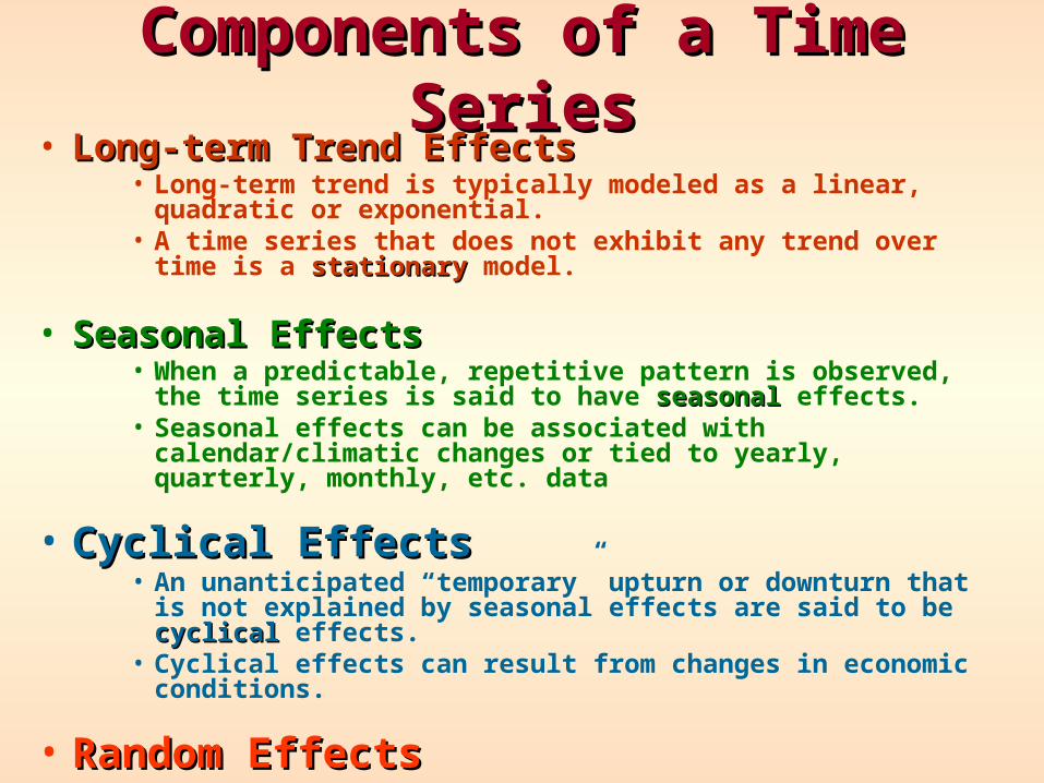
Components of a Time SeriesComponents of a Time Series• Long-term Trend EffectsLong-term Trend Effects

• Long-term trend is typically modeled as a linear, quadratic or exponential.

• A time series that does not exhibit any trend over time is a stationarystationary model.

• Seasonal EffectsSeasonal Effects • When a predictable, repetitive pattern is observed, the time

series is said to have seasonalseasonal effects.• Seasonal effects can be associated with calendar/climatic

changes or tied to yearly, quarterly, monthly, etc. data

• Cyclical EffectsCyclical Effects• An unanticipated “temporary” upturn or downturn that is not

explained by seasonal effects are said to be cyclicalcyclical effects.• Cyclical effects can result from changes in economic

conditions.

• Random EffectsRandom Effects

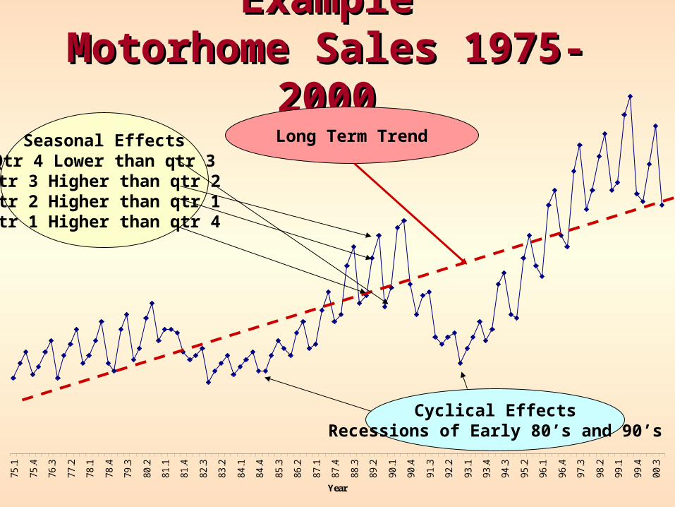
ExampleExampleMotorhome Sales 1975-2000Motorhome Sales 1975-2000

75.1

75.4

76.3

77.2

78.1

78.4

79.3

80.2

81.1

81.4

82.3

83.2

84.1

84.4

85.3

86.2

87.1

87.4

88.3

89.2

90.1

90.4

91.3

92.2

93.1

93.4

94.3

95.2

96.1

96.4

97.3

98.2

99.1

99.4

00.3

Year

Long Term TrendSeasonal EffectsQtr 4 Lower than qtr 3Qtr 3 Higher than qtr 2Qtr 2 Higher than qtr 1Qtr 1 Higher than qtr 4

Cyclical EffectsRecessions of Early 80’s and 90’s

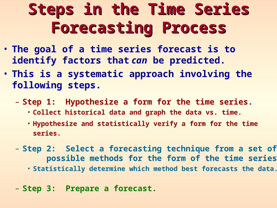
Steps in the Time Series Steps in the Time Series Forecasting ProcessForecasting Process

• The goal of a time series forecast is to identify factors that can be predicted.

• This is a systematic approach involving the following steps.

– Step 1: Hypothesize a form for the time series. • Collect historical data and graph the data vs. time.

• Hypothesize and statistically verify a form for the time series.

– Step 2: Select a forecasting technique from a set of possible methods for the form of the time

series.• Statistically determine which method best forecasts the data.

– Step 3: Prepare a forecast.

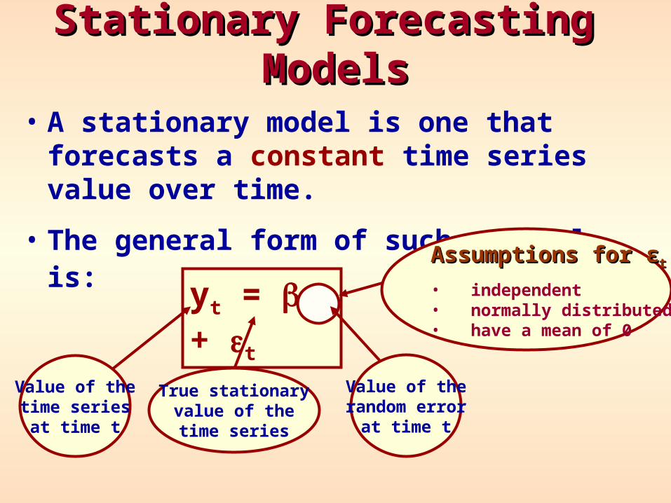
Stationary Forecasting ModelsStationary Forecasting Models

• A stationary model is one that forecasts a constant time series value over time.

• The general form of such a model is:

yt = 0 + t

Assumptions for Assumptions for εεtt

• independent• normally distributed• have a mean of 0

Value of thetime series

at time t

True stationaryvalue of thetime series

Value of therandom error

at time t

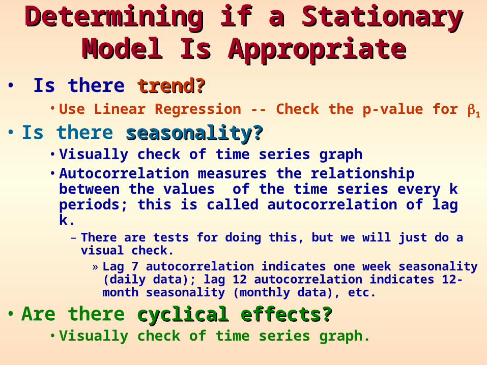
Determining if a Stationary Model Determining if a Stationary Model Is AppropriateIs Appropriate

• Is there trend?trend? • Use Linear Regression -- Check the p-value for 1

• Is there seasonality?seasonality?• Visually check of time series graph• Autocorrelation measures the relationship between

the values of the time series every k periods; this is called autocorrelation of lag k.

– There are tests for doing this, but we will just do a visual check.

» Lag 7 autocorrelation indicates one week seasonality (daily data); lag 12 autocorrelation indicates 12-month seasonality (monthly data), etc.

• Are there cyclical effects?cyclical effects?• Visually check of time series graph.

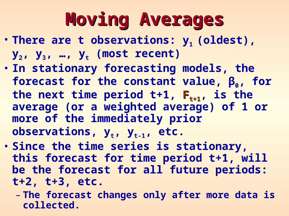
Moving AveragesMoving Averages• There are t observations: y1 (oldest), y2, y3,

…, yt (most recent)• In stationary forecasting models, the

forecast for the constant value, β0, for the next time period t+1, FFt+1t+1, is the average (or a weighted average) of 1 or more of the immediately prior observations, yt, yt-1, etc.

• Since the time series is stationary, this forecast for time period t+1, will be the forecast for all future periods: t+2, t+3, etc.– The forecast changes only after more data is

collected.

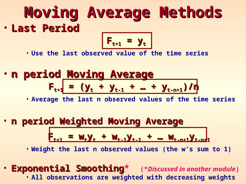
Moving Average MethodsMoving Average Methods• Last PeriodLast Period

FFt+1t+1 = y = ytt

• Use the last observed value of the time series

• n period Moving Averagen period Moving AverageFFt+1t+1 = (y = (ytt + y + yt-1t-1 + … + y + … + yt-n+1t-n+1)/n)/n

• Average the last n observed values of the time series

• n period Weighted Moving Averagen period Weighted Moving Average

FFt+1t+1 = w = wttyytt + w + wt-1t-1yyt-1t-1 + … w + … wt-n+1t-n+1yyt-n+1t-n+1

• Weight the last n observed values (the w’s sum to 1)

• Exponential SmoothingExponential Smoothing* (*Discussed in another module)• All observations are weighted with decreasing weights

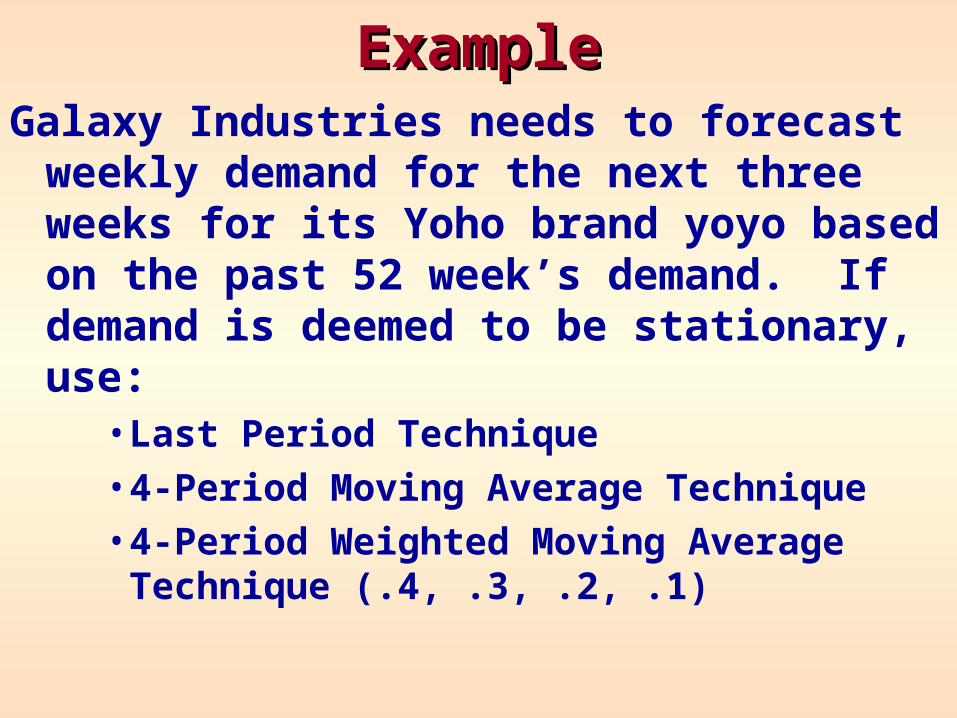
ExampleExampleGalaxy Industries needs to forecast weekly

demand for the next three weeks for its Yoho brand yoyo based on the past 52 week’s demand. If demand is deemed to be stationary, use:

• Last Period Technique• 4-Period Moving Average Technique• 4-Period Weighted Moving Average

Technique (.4, .3, .2, .1)

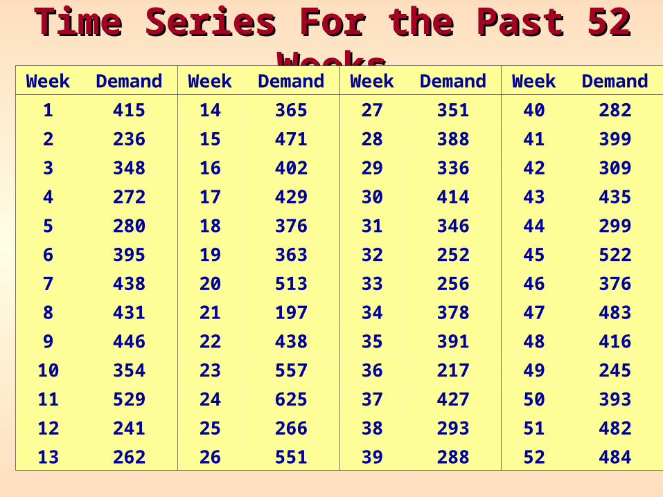
Time Series For the Past 52 WeeksTime Series For the Past 52 WeeksWeek Demand Week Demand Week Demand Week Demand

1 415 14 365 27 351 40 282

2 236 15 471 28 388 41 399

3 348 16 402 29 336 42 309

4 272 17 429 30 414 43 435

5 280 18 376 31 346 44 299

6 395 19 363 32 252 45 522

7 438 20 513 33 256 46 376

8 431 21 197 34 378 47 483

9 446 22 438 35 391 48 416

10 354 23 557 36 217 49 245

11 529 24 625 37 427 50 393

12 241 25 266 38 293 51 482

13 262 26 551 39 288 52 484

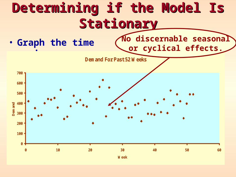
Determining if the Model Is Determining if the Model Is StationaryStationary

• Graph the time series.

Demand For Past 52 Weeks

0

100

200

300

400

500

600

700

0 10 20 30 40 50 60

Week

Dem

and

No discernable seasonalor cyclical effects.

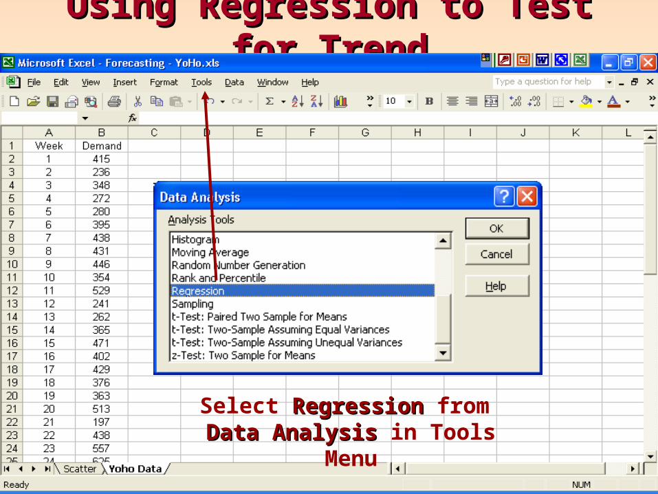
Using Regression to Test for TrendUsing Regression to Test for Trend

Select RegressionRegression from Data AnalysisData Analysis in Tools Menu

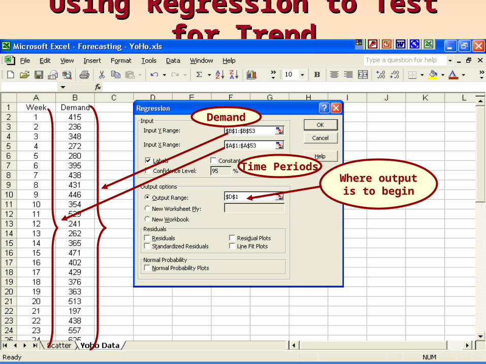
Using Regression to Test for TrendUsing Regression to Test for Trend

Where outputis to begin

Demand

Time Periods

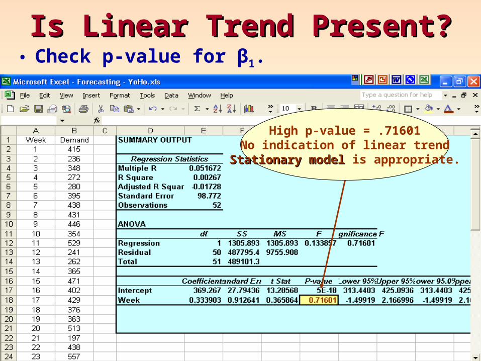
Is Linear Trend Present?Is Linear Trend Present?• Check p-value for β1.

High p-value = .71601No indication of linear trend

Stationary modelStationary model is appropriate.

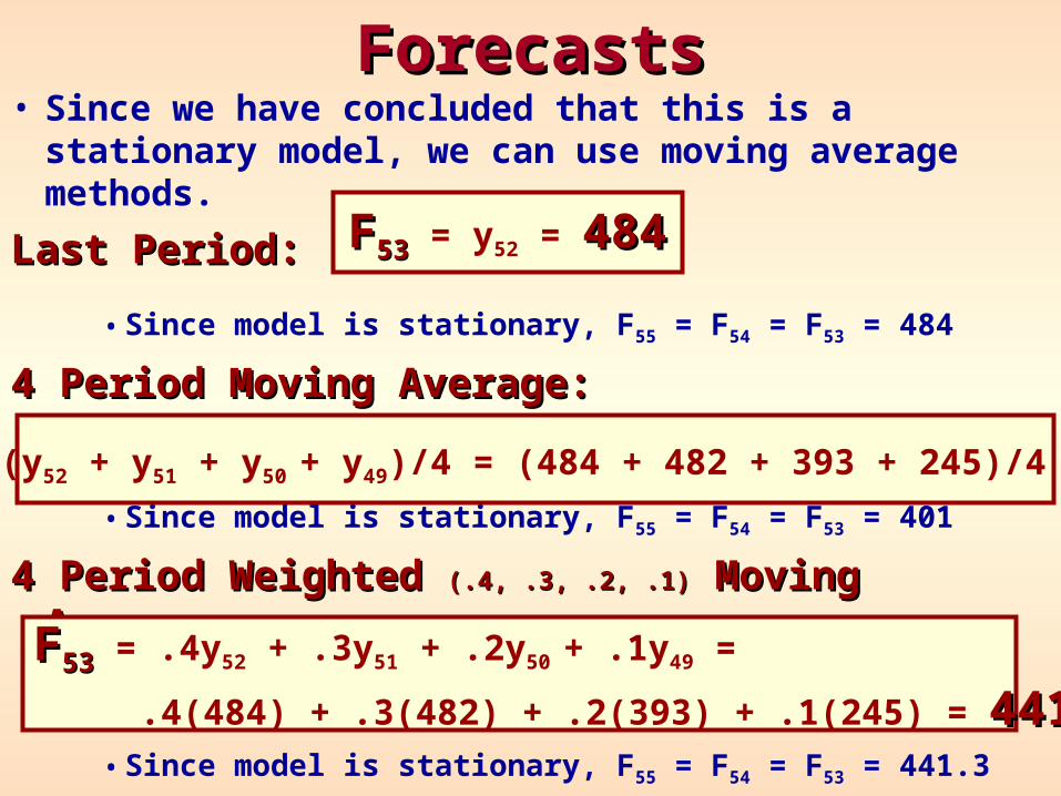
ForecastsForecasts• Since we have concluded that this is a stationary

model, we can use moving average methods.

Last Period:Last Period:

• Since model is stationary, F55 = F54 = F53 = 484

4 Period Moving Average:4 Period Moving Average:

• Since model is stationary, F55 = F54 = F53 = 401

4 Period Weighted 4 Period Weighted (.4, .3, .2, .1)(.4, .3, .2, .1) Moving Average: Moving Average:

• Since model is stationary, F55 = F54 = F53 = 441.3

FF5353 = (y52 + y51 + y50 + y49)/4 = (484 + 482 + 393 + 245)/4 = 401401

FF5353 = y52 = 484484

FF5353 = .4y52 + .3y51 + .2y50 + .1y49 =

.4(484) + .3(482) + .2(393) + .1(245) = 441.3441.3

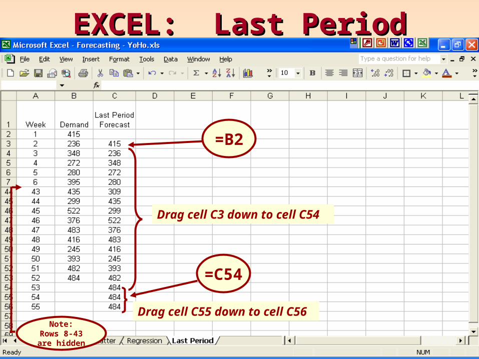
EXCEL: Last PeriodEXCEL: Last Period

Note:Rows 8-43are hidden

=B2

Drag cell C3 down to cell C54

=C54


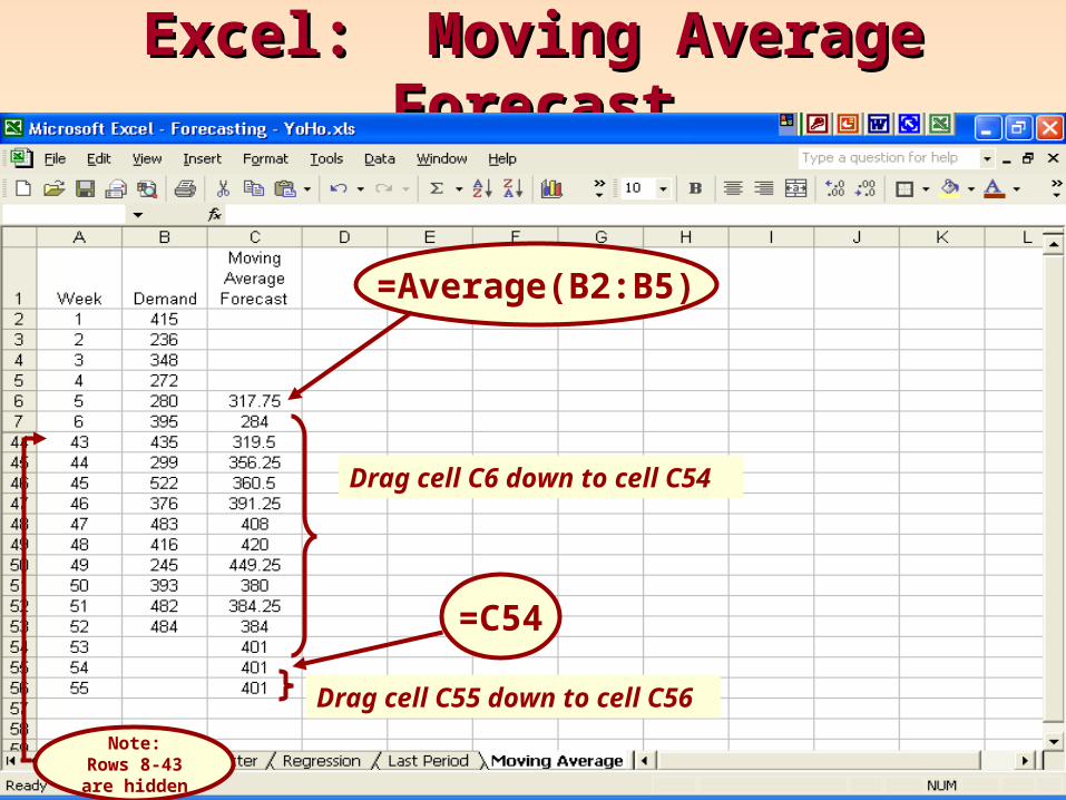
Excel: Moving Average ForecastExcel: Moving Average Forecast


=Average(B2:B5)



=C54

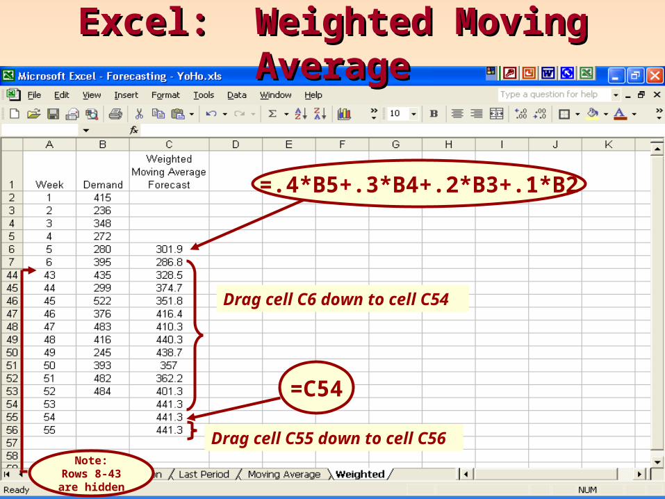
Excel: Weighted Moving AverageExcel: Weighted Moving Average

=.4*B5+.3*B4+.2*B3+.1*B2



=C54


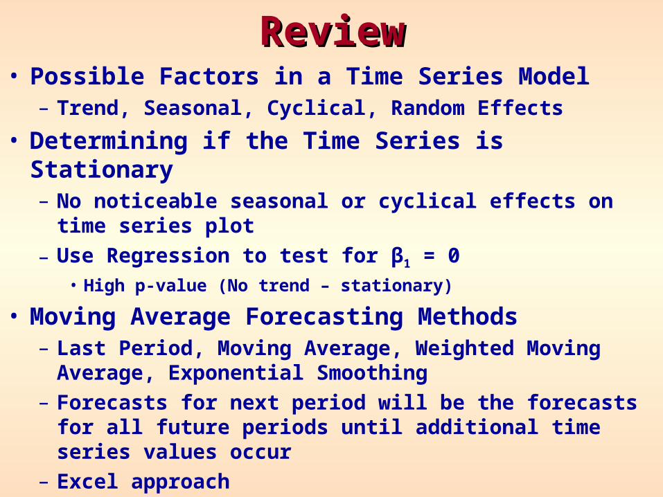
ReviewReview• Possible Factors in a Time Series Model

– Trend, Seasonal, Cyclical, Random Effects

• Determining if the Time Series is Stationary– No noticeable seasonal or cyclical effects on time series

plot

– Use Regression to test for β1 = 0• High p-value (No trend – stationary)

• Moving Average Forecasting Methods– Last Period, Moving Average, Weighted Moving

Average, Exponential Smoothing– Forecasts for next period will be the forecasts for all

future periods until additional time series values occur– Excel approach

forecasting basic concepts basic conceptsand stationary models

Documents