functional analysis - tokyo metropolitan …1 functional analysis 1.1 normed spaces 1.1.1...
TRANSCRIPT
FUNCTIONAL ANALYSIS
Okazaki Junichiro
平成 16 年 4 月 17 日

概 要
SPACES
Linear spaces : just a module (algebraic system)SNormed spaces : a module with geometrical property, normSBanach spaces : completenessSHilbert spaces : inner product (orthogonality)S
Euclidean spaces :
i

目 次1 Functional analysis 1
1.1 Normed spaces . . . . . . . . . . . . . . . . . . . . . . . . . . . . . . . . . . . . . 11.1.1 Definition of LINEAR SPACE . . . . . . . . . . . . . . . . . . . . . . . . 11.1.2 Definition of NORM . . . . . . . . . . . . . . . . . . . . . . . . . . . . . . 3
1.2 Some Normed Space . . . . . . . . . . . . . . . . . . . . . . . . . . . . . . . . . . 41.2.1 Definition of lp . . . . . . . . . . . . . . . . . . . . . . . . . . . . . . . . . 41.2.2 Definition of l∞ . . . . . . . . . . . . . . . . . . . . . . . . . . . . . . . . . 41.2.3 Definition of c0 . . . . . . . . . . . . . . . . . . . . . . . . . . . . . . . . . 41.2.4 Definition of Lp . . . . . . . . . . . . . . . . . . . . . . . . . . . . . . . . . 51.2.5 Definition of L∞ . . . . . . . . . . . . . . . . . . . . . . . . . . . . . . . . 51.2.6 Definition of C([0, 1]) . . . . . . . . . . . . . . . . . . . . . . . . . . . . . 51.2.7 Definition of C0 . . . . . . . . . . . . . . . . . . . . . . . . . . . . . . . . . 51.2.8 Definition of Cc . . . . . . . . . . . . . . . . . . . . . . . . . . . . . . . . . 51.2.9 Definition of C∞([0, 1]) . . . . . . . . . . . . . . . . . . . . . . . . . . . . 5
1.3 Banach space & Hilbert space . . . . . . . . . . . . . . . . . . . . . . . . . . . . . 61.3.1 Definition of BANACH SPACE . . . . . . . . . . . . . . . . . . . . . . . . 61.3.2 Theorem; Normed space l2 is complete . . . . . . . . . . . . . . . . . . . . 71.3.3 Definition of INNER PRODUCT . . . . . . . . . . . . . . . . . . . . . . . 81.3.4 Lemma (Schwartz’s inequality) . . . . . . . . . . . . . . . . . . . . . . . . 91.3.5 Theorem . . . . . . . . . . . . . . . . . . . . . . . . . . . . . . . . . . . . 101.3.6 Definition of HILBERT SPACE . . . . . . . . . . . . . . . . . . . . . . . . 111.3.7 Theorem (von Neumann) . . . . . . . . . . . . . . . . . . . . . . . . . . . 121.3.8 Lemma (Holder’s inequality) . . . . . . . . . . . . . . . . . . . . . . . . . 141.3.9 Lemma (Minkowski’s inequality) . . . . . . . . . . . . . . . . . . . . . . . 15
1.4 Linear Operator . . . . . . . . . . . . . . . . . . . . . . . . . . . . . . . . . . . . 161.4.1 Definition of LINEAR OPERATOR . . . . . . . . . . . . . . . . . . . . . 161.4.2 Definition of CONTINUOUS . . . . . . . . . . . . . . . . . . . . . . . . . 161.4.3 Definition of BOUNDED . . . . . . . . . . . . . . . . . . . . . . . . . . . 161.4.4 Definition of OPERATOR NORM . . . . . . . . . . . . . . . . . . . . . . 161.4.5 Theorem . . . . . . . . . . . . . . . . . . . . . . . . . . . . . . . . . . . . 171.4.6 Lemma . . . . . . . . . . . . . . . . . . . . . . . . . . . . . . . . . . . . . 181.4.7 Theorem . . . . . . . . . . . . . . . . . . . . . . . . . . . . . . . . . . . . 191.4.8 Theorem . . . . . . . . . . . . . . . . . . . . . . . . . . . . . . . . . . . . 20
1.5 Banach-Bernstein’s Theorem . . . . . . . . . . . . . . . . . . . . . . . . . . . . . 211.5.1 Banach-Bernstein’s Theorem . . . . . . . . . . . . . . . . . . . . . . . . . 21
1.6 Baire’s Category Theorem 1, 2 . . . . . . . . . . . . . . . . . . . . . . . . . . . . 221.6.1 Baire’s Category Theorem 1 . . . . . . . . . . . . . . . . . . . . . . . . . . 221.6.2 Baire’s Category Theorem 2 . . . . . . . . . . . . . . . . . . . . . . . . . . 231.6.3 Proposition . . . . . . . . . . . . . . . . . . . . . . . . . . . . . . . . . . . 241.6.4 Proposition . . . . . . . . . . . . . . . . . . . . . . . . . . . . . . . . . . . 251.6.5 Theorem . . . . . . . . . . . . . . . . . . . . . . . . . . . . . . . . . . . . 26
ii
1.6.6 Corollary . . . . . . . . . . . . . . . . . . . . . . . . . . . . . . . . . . . . 271.6.7 Pettis-Plesner’s theorem . . . . . . . . . . . . . . . . . . . . . . . . . . . . 27
1.7 Hahn-Banach’s theorem on R . . . . . . . . . . . . . . . . . . . . . . . . . . . . . 281.7.1 Hahn-Banach’s theorem . . . . . . . . . . . . . . . . . . . . . . . . . . . . 281.7.2 Lemma . . . . . . . . . . . . . . . . . . . . . . . . . . . . . . . . . . . . . 301.7.3 . . . . . . . . . . . . . . . . . . . . . . . . . . . . . . . . . . . . . . . . . 321.7.4 . . . . . . . . . . . . . . . . . . . . . . . . . . . . . . . . . . . . . . . . . 321.7.5 Riesz’s representation theorem . . . . . . . . . . . . . . . . . . . . . . . . 331.7.6 . . . . . . . . . . . . . . . . . . . . . . . . . . . . . . . . . . . . . . . . . 341.7.7 . . . . . . . . . . . . . . . . . . . . . . . . . . . . . . . . . . . . . . . . . 341.7.8 . . . . . . . . . . . . . . . . . . . . . . . . . . . . . . . . . . . . . . . . . 341.7.9 . . . . . . . . . . . . . . . . . . . . . . . . . . . . . . . . . . . . . . . . . 341.7.10 . . . . . . . . . . . . . . . . . . . . . . . . . . . . . . . . . . . . . . . . . 341.7.11 . . . . . . . . . . . . . . . . . . . . . . . . . . . . . . . . . . . . . . . . . 341.7.12 . . . . . . . . . . . . . . . . . . . . . . . . . . . . . . . . . . . . . . . . . 341.7.13 . . . . . . . . . . . . . . . . . . . . . . . . . . . . . . . . . . . . . . . . . 341.7.14 . . . . . . . . . . . . . . . . . . . . . . . . . . . . . . . . . . . . . . . . . 341.7.15 . . . . . . . . . . . . . . . . . . . . . . . . . . . . . . . . . . . . . . . . . 341.7.16 . . . . . . . . . . . . . . . . . . . . . . . . . . . . . . . . . . . . . . . . . 341.7.17 . . . . . . . . . . . . . . . . . . . . . . . . . . . . . . . . . . . . . . . . . 341.7.18 . . . . . . . . . . . . . . . . . . . . . . . . . . . . . . . . . . . . . . . . . 341.7.19 . . . . . . . . . . . . . . . . . . . . . . . . . . . . . . . . . . . . . . . . . 341.7.20 . . . . . . . . . . . . . . . . . . . . . . . . . . . . . . . . . . . . . . . . . 341.7.21 . . . . . . . . . . . . . . . . . . . . . . . . . . . . . . . . . . . . . . . . . 34
iii

1 Functional analysis
1.1 Normed spaces
1.1.1 Definition of LINEAR SPACE
Review; R-module
R: a ring 1 (commutative 1 ∈ R) (← defined with operation , +, × )
M : R-module def⇐⇒(1) M is an abelian2 w.r.t. addition.(2) R×M −→ M : scalar multiplication s.t.for any r, r′ ∈ R, m,m′ ∈M
1. (r + r′)m = rm+ r′m
2. (rr′)m = r(r′m)
3. r(m+m′) = rm+ rm′
4. 1 ·m = m
If R is a field, then M is called a vecter space over R.
1G; a group
G×Ginner operation−−−−−−−−−−→ G
(g1, g2) 7−→ g1g2
1. associativity
2. an identity element
3. the inverse element
R; a ring
R×Rinner operation−−−−−−−−−−→ R¡
(r1, r2) 7−→ r1 + r2 ; say addition(r1, r2) 7−→ r1r2 ; say multiplication
and R is an abelian group w.r.t. additionR is a monoid w.r.t. multiplication (Semi-group ⊂ Monoid ⊂ Group)
moreover, R satisfies the distributivity;r1(r2 + r3) = r1r2 + r1r3
M ; R-module
M ×Minner operation−−−−−−−−−−→ M
(m1, m2) 7−→ m1 + m2 ; say addition
R×Mouter operation−−−−−−−−−−−→ M
(r, m) 7−→ rm ; say scalar multiplication
2(M ,+):an abelian group ⇔ Addition is definded on M , and satisfies the following conditions;
1. associativity; m + (m′ + m′′) = (m + m′) + m′′
2. an identity element; ∃0 ∈ M s.t. 0 + m = m
3. the inverse element; ∀m ∈ M, ∃ −m ∈ M s.t. m + (−m) = 0
4. commutativty; m + m′ = m′ + m
1

1. Functional analysis
Example
When M = R, M is a module over R.R×M −→ M
ExampleA; an abelian grp.R = Z; the ring of intergersn ∈ Z, a ∈ A
na =def
a+ a+ · · ·+ a if n > 00 if n = 0
(−a) + (−a) + · · ·+ (−a) if n < 0
Then A is a module in Z.
abelian group = Z-module (module over Z)
2
1.1. Normed spaces
E is called a vector space, or linear space, if it is a module over fieldK, on which addition(inner operation)& scalar multiplication(outer operation) is defined.
1.1.2 Definition of NORM
E; a vector space∀ x ∈ E
‖ · ‖ : E −→ R≥0
1. ‖x‖ ≥ 0, ‖x‖ = 0 ⇐⇒ x = 0
2. ‖αx‖ = |α|‖x‖
3. ‖x+ y‖ ≤ ‖x‖+ ‖y‖
Then we call ‖ · ‖ norm , and if it does not satisfy ‖x‖ = 0⇔ x = 0, we call it semi-norm.
The pair (E, ‖ · ‖E) is called a normed space.
3

1. Functional analysis
1.2 Some Normed Space
1.2.1 Definition of lp
lp = {x = (x1, x2, · · · , xn, · · · ) | ‖x‖p ; finite} is a vect. sp. and is normed with
‖x‖p =def
( ∞∑n=1
|xn|p) 1
p
1.2.2 Definition of l∞
l∞ = {x = (x1, x2, · · · , xn, · · · ) | ‖x‖∞ ; finite} is a vect. sp. and is normed with
‖x‖∞ =def
sup1≤n<∞
|xn|
1.2.3 Definition of c0
c0 = {x = (x1, x2, · · · , xn, · · · ) | xj −−−−→j−→∞
0} is a vect. sp. and is normed with
‖x‖∞ =def
sup1≤n<∞
|xn|
4
1.2. Some Normed Space
1.2.4 Definition of Lp
Lp(X,µ) ={f : X −→ C | ∫
X|f(x)|pdµ(x); finite
}/ {f(x) = 0 µ− a.e.} is a vect. sp. and
is normed with
‖[f ]‖p =def
(∫
X
|f(x)|pdµ(x)) 1
p
1.2.5 Definition of L∞
L∞(X,µ) = {f : essentially bounded} / {f(x) = 0 µ−a.e.} is a vect. sp. and is normed with
‖[f ]‖∞ def= ess.sup|f(x)|def= inf
[α | µ
({x ∈ X | |f(x)| > α
})= 0
]
1.2.6 Definition of C([0, 1])
C([0, 1]) = { f : [0, 1] −→ C | continuous} is a vect. sp. and is normed with
‖f‖∞ = max0≤x≤1
|f(x)|
1.2.7 Definition of C0
C0(R) = {f : R −→ R | continuous, |f(x)| −−−−−→|x|−→∞
0} is a vect. sp. and is normed with
‖f‖∞ = supR|f |
1.2.8 Definition of Cc
Cc = {f ∈ C0 | suppf ; compact}
1.2.9 Definition of C∞([0, 1])
C∞([0, 1]) = {f : [0, 1] −→ R | C∞ − class} is a vect. sp. and is normed with
‖f‖∞ = sup0≤x≤1
|f(x)|
5

1. Functional analysis
1.3 Banach space & Hilbert space
1.3.1 Definition of BANACH SPACE
(E, ‖ · ‖E); Banach space
⇐⇒ E; complete3 w.r.t. T‖·‖E
Example;Every finite dimensional normed space is Banach space.
Remark
lp, l∞, c0, Lp, L∞, C0 are Banach spaces.
Cc(R), C∞([0, 1]) are not Banach spaces.
3i.e. Any Cauchy sequence converges in E
6

1.3. Banach space & Hilbert space
1.3.2 Theorem; Normed space l2 is complete
7
1. Functional analysis
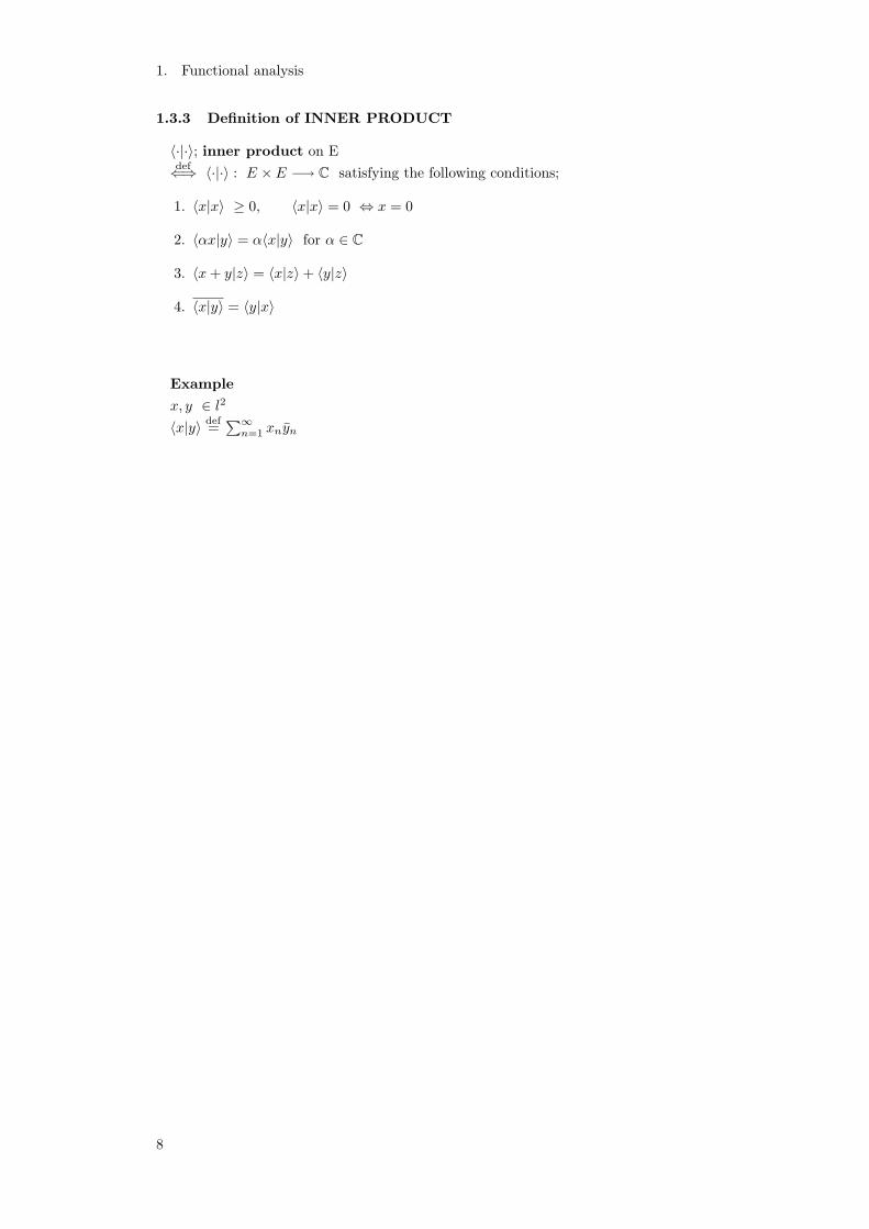
1.3.3 Definition of INNER PRODUCT
〈·|·〉; inner product on Edef⇐⇒ 〈·|·〉 : E × E −→ C satisfying the following conditions;
1. 〈x|x〉 ≥ 0, 〈x|x〉 = 0 ⇔ x = 0
2. 〈αx|y〉 = α〈x|y〉 for α ∈ C
3. 〈x+ y|z〉 = 〈x|z〉+ 〈y|z〉
4. 〈x|y〉 = 〈y|x〉
Example
x, y ∈ l2〈x|y〉 def=
∑∞n=1 xnyn
8
1.3. Banach space & Hilbert space
1.3.4 Lemma (Schwartz’s inequality)
(E, 〈·|·〉E); an inner product space
|〈x|y〉E | ≤ ‖x‖E‖y‖E for any x, y ∈ E
9
1. Functional analysis
1.3.5 Theorem
(E, 〈·|·〉E); an inner product space
Then
1. ‖x‖E def= (〈x|x〉E)12 satisfies the properties of norm.
2. ‖x+ y‖2E + ‖x− y‖2E = 2(‖x‖2E + ‖y‖2E)
10
1.3. Banach space & Hilbert space
1.3.6 Definition of HILBERT SPACE
(E, 〈·|·〉E); Hilbert space
def⇐⇒ (E, ‖ · ‖E); Banach space, here ‖ · ‖E = (〈·|·〉E)12
11
1. Functional analysis
1.3.7 Theorem (von Neumann)
∃ inner product 〈·|·〉 on E s.t.√〈x|x〉E = ‖x‖E
⇐⇒ ‖x+ y‖2E + ‖x− y‖2E = 2(‖x‖2E + ‖y‖2E) for any x, y ∈ E
12

1.3. Banach space & Hilbert space
proof
13

1. Functional analysis
◎ Inequalties
1.3.8 Lemma (Holder’s inequality)
1 < p <∞
q =p
p− 14
f ∈ Lp(X)
g ∈ Lq(X)
Then, ∣∣∣∣∫
X
f(x)g(x)dx∣∣∣∣ ≤ ‖f‖p‖g‖q
4
1
p+
1
q= 1
14

1.3. Banach space & Hilbert space
1.3.9 Lemma (Minkowski’s inequality)
1 ≤ p <∞f, g ∈ Lp(X) =⇒ f + g ∈ Lp(X)
Moreover,
(∫
X
|f(x) + g(x)|pdx) 1
p
≤(∫
X
|f(x)|pdx) 1
p
+(∫
X
|g(x)|pdx) 1
p
15

1. Functional analysis
1.4 Linear Operator
(E, ‖ · ‖E) T−−−→linear
(F, ‖ · ‖F )
finite ⇒ T ;matrix
infinite ⇒ ???
1.4.1 Definition of LINEAR OPERATOR
(E, ‖ · ‖E), (F, ‖ · ‖F ); normed space
T : E −→ F ; linear operator def⇐⇒ T (αx+ βy) = αTx+ βTy
NOTATION
L(E,F ) def= {T | T : E −→ F ; linear}and, if E = F , L(E,F ) is denoted by L(E).
1.4.2 Definition of CONTINUOUS
T ∈ L(E,F )
T ; continuous on E def⇐⇒ ‖xn − x‖ −→n→∞
0 ⇒ ‖Txn − Tx‖ −→n→∞
0
1.4.3 Definition of BOUNDED
T ∈ L(E,F )
T ; bounded on E def⇐⇒ ∃K > 0 s.t. ‖Tx‖F ≤ K‖x‖E for any x ∈ E
NOTATION
B(E,F ) def= {T ∈ L(E,F ) | T ; bounded}
1.4.4 Definition of OPERATOR NORM
∀ T ∈ B(E,F )
‖T‖ def= inf{K > 0 | ||Tx||F ≤ K‖x‖E for any x ∈ E}
; called operator norm, uniform norm
16

1.4. Linear Operator
1.4.5 Theorem
E, F ; normed space
=⇒ (B(E,F ), ‖ · ‖) ; normed space
17
1. Functional analysis
1.4.6 Lemma
γ1 =def
sup0 6=x∈E
‖Tx‖F‖x‖E
γ2 =def
sup‖x‖E=1
‖Tx‖F
γ3 =def
sup‖x‖E<1
‖Tx‖F
Then γ1 = γ2 = γ3 = ‖T‖
18
1.4. Linear Operator
1.4.7 Theorem
T ∈ L(E,F )
Then the following conditions are equivalent;
1. T ; conti. on E
2. T ; conti. at 0
3. T ; bounded
19

1. Functional analysis
1.4.8 Theorem
F ; Banach space =⇒ B(E,F ); Banach space
20
1.5. Banach-Bernstein’s Theorem
1.5 Banach-Bernstein’s Theorem
1.5.1 Banach-Bernstein’s Theorem
(Uniform Bounded Theorem)E,F ; normed spaceE; Banach spaceB(E,F ) 3 T : E −→ F ; bounded linear operatorA ⊂ B(E,F ); a non-empty subset of B(E,F )
∀x ∈ E (fixed.), supT∈A ‖Tx‖F ; finite (strong operator topology) on B(E,F )
=⇒ supT∈A ‖T‖; finite (uniform operator topology) on B(E,F ) 5
Proof∀n ≥ 1Put Cn = { x ∈ E | ‖Tx‖F ≤ n for any T ∈ A }∀x ∈ E, ∃n ∈ N, s.t. supT∈A ‖Tx‖F ≤ n by assumption=⇒ ‖Tx‖F ≤ n for every T ∈ A=⇒ x ∈ Cn
=⇒ E ⊂ ⋃∞n=1 Cn
=⇒ E =⋃∞
n=1 Cn
claim; Cn; closed in E.Furthermore, since E is a Banach space
5A; strongly operator bounded =⇒ A; uniformly operator bounded
Remark;
E, F ; finite dimensional =⇒ (s)-top. = (u)-top.
21
1. Functional analysis
1.6 Baire’s Category Theorem 1, 2
1.6.1 Baire’s Category Theorem 1
(X, d); complete metric spaceOn ⊂ X; open dense6 in X
=⇒ ⋂∞n=1On; dense in X
6i.e. On = X
22

1.6. Baire’s Category Theorem 1, 2
1.6.2 Baire’s Category Theorem 2
(X, d); complete metric spaceCn; closed in XX =
⋃∞n=1 Cn
=⇒ ∃m ≥ s.t. Int(Cm) 6= ∅
23
1. Functional analysis
1.6.3 Proposition
(E, ‖ · ‖); Banach space
24
1.6. Baire’s Category Theorem 1, 2
1.6.4 Proposition
p, q ∈ R≥1
p < q =⇒ lp ⊂ lq
25
1. Functional analysis
1.6.5 Theorem
1p
+1q
= 1, (p, q > 1) =⇒ (l∞, ‖ · ‖p)∗ = lp
26

1.6. Baire’s Category Theorem 1, 2
1.6.6 Corollary
p = 0, 1(l1)∗ ∼= l∞
(l∞)∗ ∼= l1
then(C0)∗∗ ∼= l∞
(C0)∗∗∗ ∼= l∞ ⊃ (C0)∗ = l1
1.6.7 Pettis-Plesner’s theorem
(E, ‖ · ‖E); Banach spaceE∗ ⊂ E∗∗∗
=⇒ E∗∗∗ = E∗ ⊕l1 E⊥
where E⊥ = { f ∈ E∗∗∗ | f |E = 0 }
27
1. Functional analysis
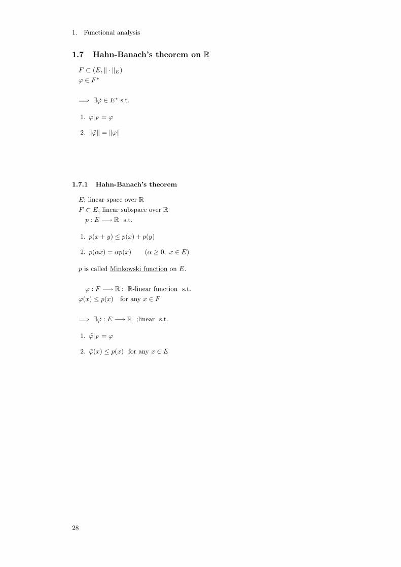
1.7 Hahn-Banach’s theorem on R
F ⊂ (E, ‖ · ‖E)ϕ ∈ F ∗
=⇒ ∃ϕ ∈ E∗ s.t.
1. ϕ|F = ϕ
2. ‖ϕ‖ = ‖ϕ‖
1.7.1 Hahn-Banach’s theorem
E; linear space over RF ⊂ E; linear subspace over Rp : E −→ R s.t.
1. p(x+ y) ≤ p(x) + p(y)
2. p(αx) = αp(x) (α ≥ 0, x ∈ E)
p is called Minkowski function on E.
ϕ : F −→ R : R-linear function s.t.ϕ(x) ≤ p(x) for any x ∈ F
=⇒ ∃ϕ : E −→ R ;linear s.t.
1. ϕ|F = ϕ
2. ϕ(x) ≤ p(x) for any x ∈ E
28

1.7. Hahn-Banach’s theorem on R
(proof)
29
1. Functional analysis
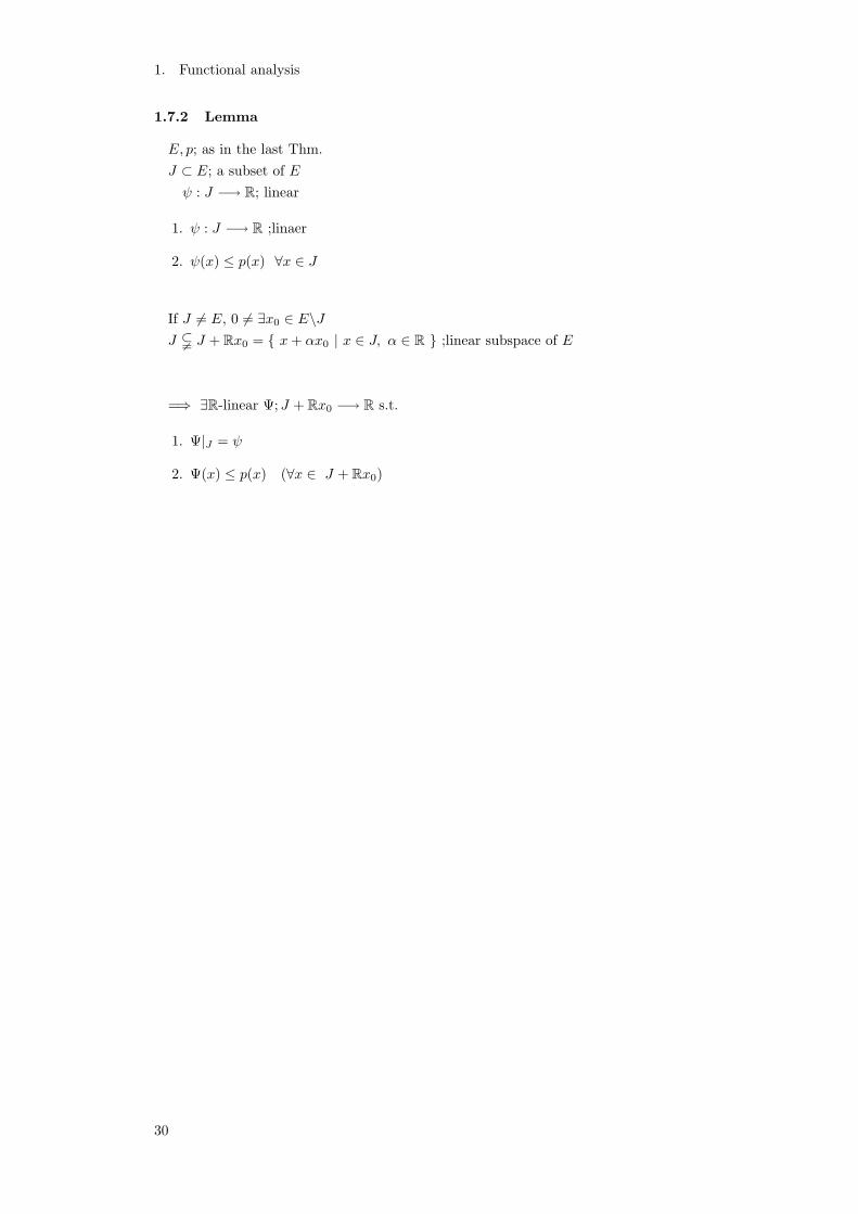
1.7.2 Lemma
E, p; as in the last Thm.J ⊂ E; a subset of Eψ : J −→ R; linear
1. ψ : J −→ R ;linaer
2. ψ(x) ≤ p(x) ∀x ∈ J
If J 6= E, 0 6= ∃x0 ∈ E\JJ $ J + Rx0 = { x+ αx0 | x ∈ J, α ∈ R } ;linear subspace of E
=⇒ ∃R-linear Ψ;J + Rx0 −→ R s.t.
1. Ψ|J = ψ
2. Ψ(x) ≤ p(x) (∀x ∈ J + Rx0)
30

1.7. Hahn-Banach’s theorem on R
(proof)
31

1. Functional analysis
1.7.3
1.7.4
32
1.7. Hahn-Banach’s theorem on R
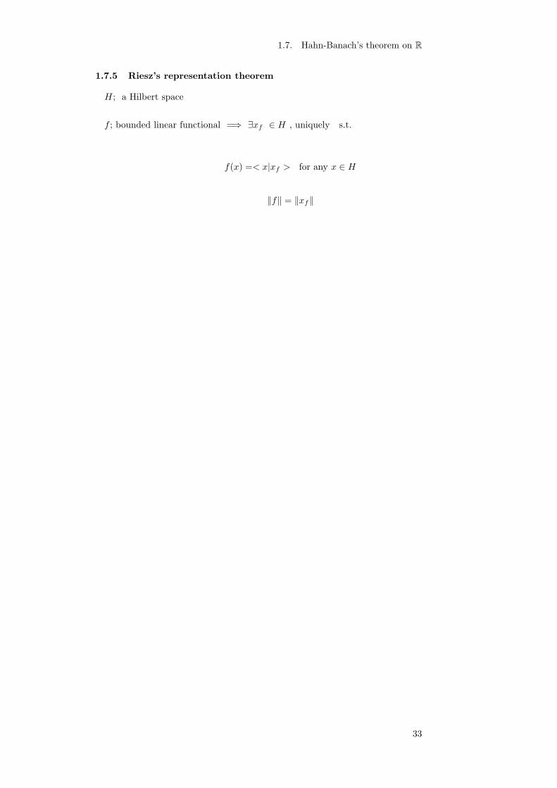
1.7.5 Riesz’s representation theorem
H; a Hilbert space
f ; bounded linear functional =⇒ ∃xf ∈ H , uniquely s.t.
f(x) =< x|xf > for any x ∈ H
‖f‖ = ‖xf‖
33

1. Functional analysis
1.7.6
1.7.7
1.7.8
1.7.9
1.7.10
1.7.11
1.7.12
1.7.13
1.7.14
1.7.15
1.7.16
1.7.17
1.7.18
1.7.19
1.7.20
1.7.21
34