giacomo boracchi - cvpr usi 2020
TRANSCRIPT
Giacomo Boracchi
Single-View GeometryGiacomo Boracchi
February 25th, 2020
USI, Lugano
Book: HZ, chapter 2
Giacomo Boracchi
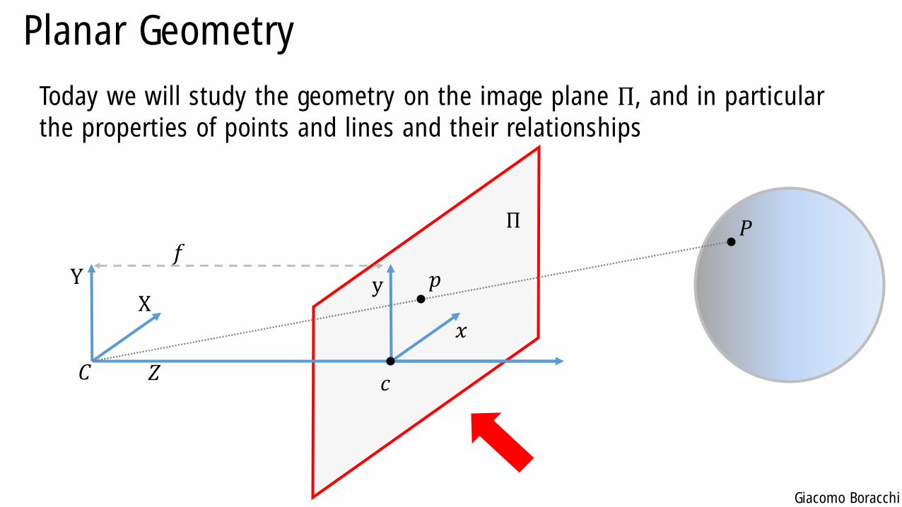
Planar Geometry
Today we will study the geometry on the image plane Π, and in particular
the properties of points and lines and their relationships
XY
𝑍𝐶 𝑐
𝑓
𝑥
y
𝑃
𝑝
Π
Giacomo Boracchi
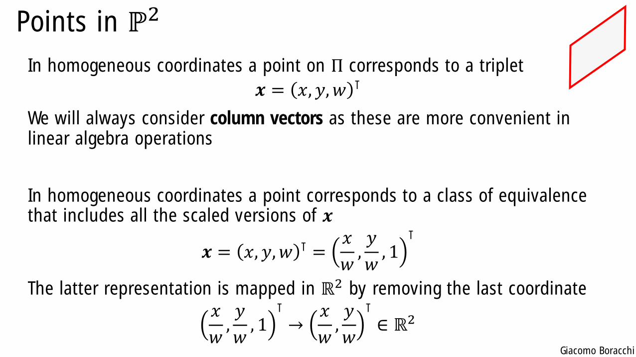
Points in ℙ2
In homogeneous coordinates a point on Π corresponds to a triplet
𝒙 = 𝑥, 𝑦, 𝑤 ⊺
We will always consider column vectors as these are more convenient in
linear algebra operations
In homogeneous coordinates a point corresponds to a class of equivalence that includes all the scaled versions of 𝒙
𝒙 = 𝑥, 𝑦, 𝑤 ⊺ =𝑥
𝑤,𝑦
𝑤, 1
⊺
The latter representation is mapped in ℝ2 by removing the last coordinate
𝑥
𝑤,𝑦
𝑤, 1
⊺
→𝑥
𝑤,𝑦
𝑤
⊺
∈ ℝ2
Giacomo Boracchi
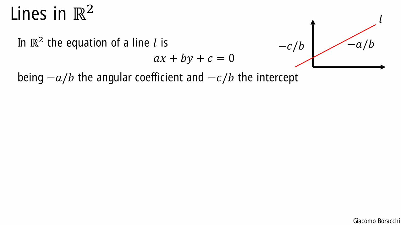
Lines in ℝ2
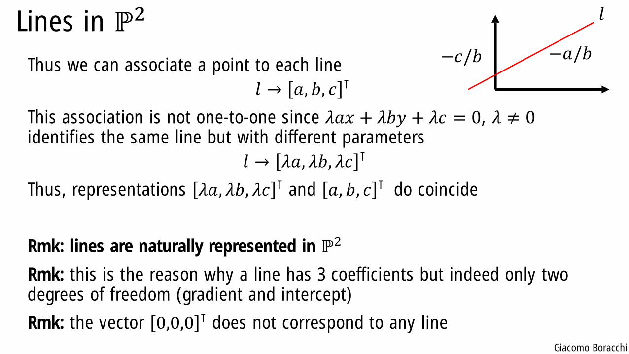
In ℝ2 the equation of a line 𝑙 is
𝑎𝑥 + 𝑏𝑦 + 𝑐 = 0
being −𝑎/𝑏 the angular coefficient and −𝑐/𝑏 the intercept
𝑙
−𝑎/𝑏−𝑐/𝑏
Giacomo Boracchi
Lines in ℙ2
Thus we can associate a point to each line
𝑙 → 𝑎, 𝑏, 𝑐 ⊺
This association is not one-to-one since 𝜆𝑎𝑥 + 𝜆𝑏𝑦 + 𝜆𝑐 = 0, 𝜆 ≠ 0identifies the same line but with different parameters
𝑙 → 𝜆𝑎, 𝜆𝑏, 𝜆𝑐 ⊺
Thus, representations 𝜆𝑎, 𝜆𝑏, 𝜆𝑐 ⊺ and 𝑎, 𝑏, 𝑐 ⊺ do coincide
Rmk: lines are naturally represented in ℙ2
Rmk: this is the reason why a line has 3 coefficients but indeed only two
degrees of freedom (gradient and intercept)
Rmk: the vector 0,0,0 ⊺ does not correspond to any line
𝑙
−𝑎/𝑏−𝑐/𝑏
Giacomo Boracchi
Incidence relation
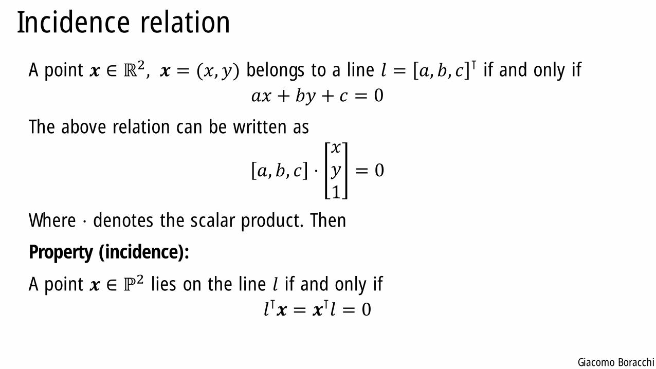
A point 𝒙 ∈ ℝ2, 𝒙 = (𝑥, 𝑦) belongs to a line 𝑙 = 𝑎, 𝑏, 𝑐 ⊺ if and only if
𝑎𝑥 + 𝑏𝑦 + 𝑐 = 0
The above relation can be written as
𝑎, 𝑏, 𝑐 ⋅𝑥𝑦1
= 0
Where ⋅ denotes the scalar product. Then
Property (incidence):
A point 𝒙 ∈ ℙ2 lies on the line 𝑙 if and only if
𝑙⊺𝒙 = 𝒙⊺𝑙 = 0
Giacomo Boracchi
Incidence relation
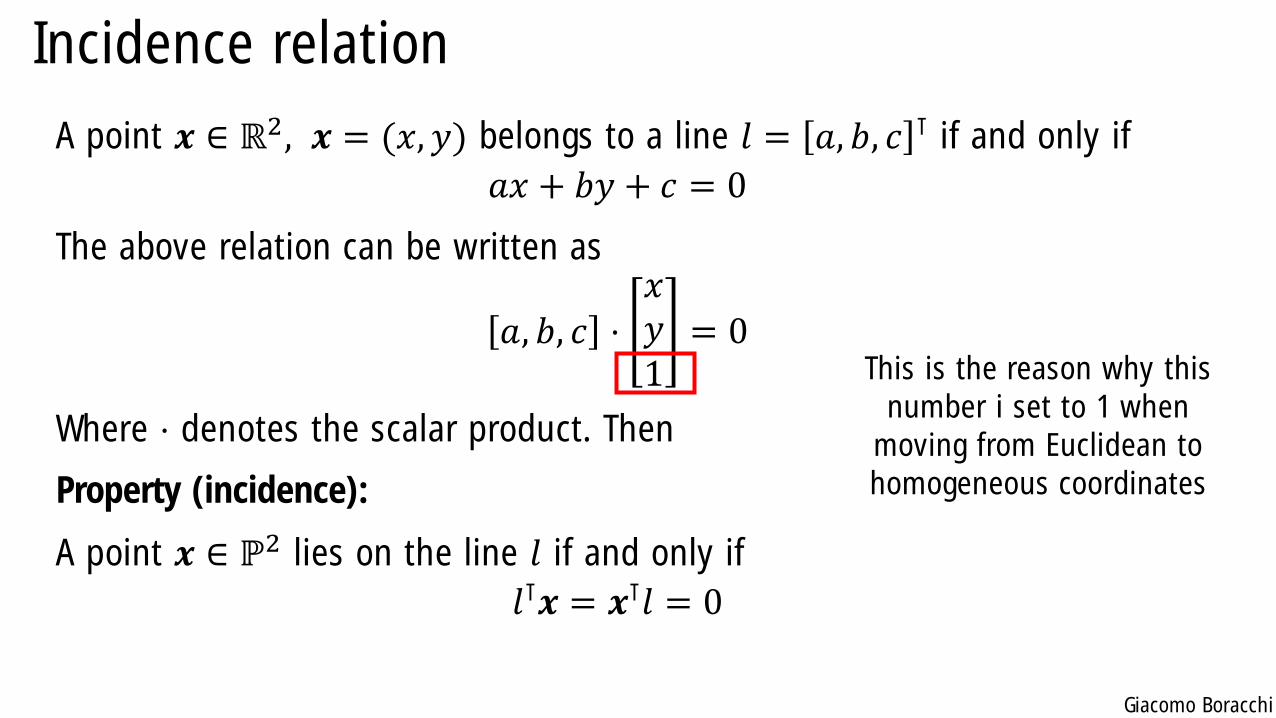
A point 𝒙 ∈ ℝ2, 𝒙 = (𝑥, 𝑦) belongs to a line 𝑙 = 𝑎, 𝑏, 𝑐 ⊺ if and only if
𝑎𝑥 + 𝑏𝑦 + 𝑐 = 0
The above relation can be written as
𝑎, 𝑏, 𝑐 ⋅𝑥𝑦1
= 0
Where ⋅ denotes the scalar product. Then
Property (incidence):
A point 𝒙 ∈ ℙ2 lies on the line 𝑙 if and only if
𝑙⊺𝒙 = 𝒙⊺𝑙 = 0
This is the reason why this
number i set to 1 when
moving from Euclidean to
homogeneous coordinates
Giacomo Boracchi
Intersection of lines
Property (intersection of lines):
The intersection of two lines 𝑙, 𝑚, their intersection 𝒙 ∈ ℙ2 is
𝒙 = 𝑙 × 𝑚
where × denote the cross product of two 3-dimensional vectors.
Giacomo Boracchi
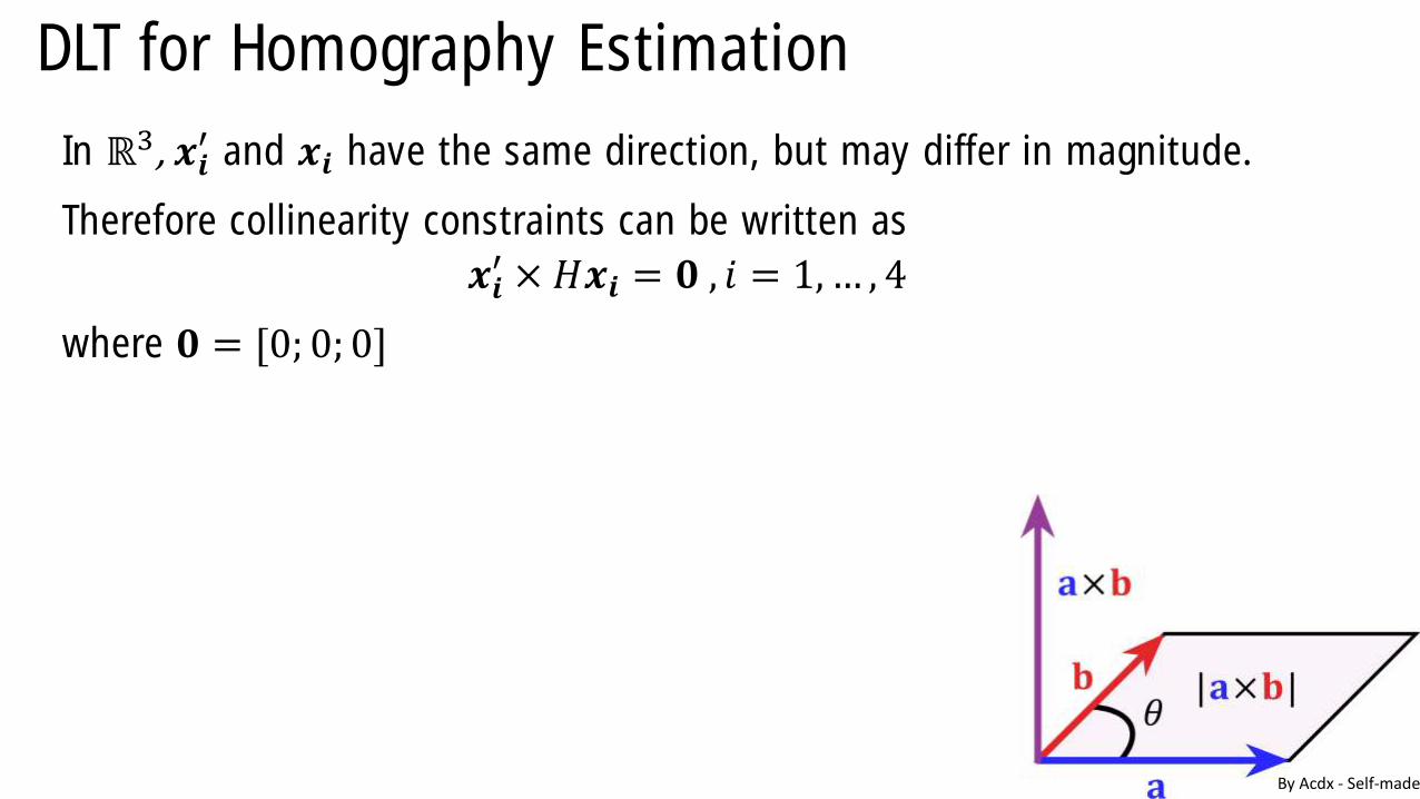
Cross Product
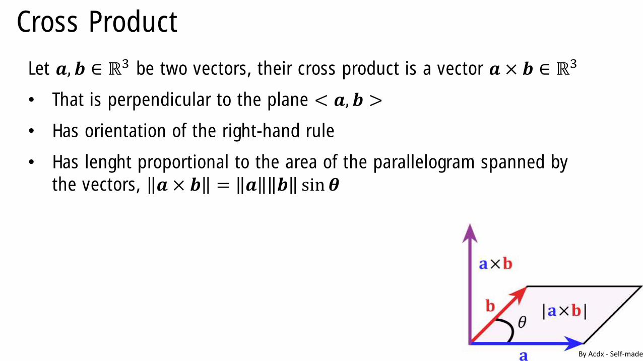
Let 𝒂, 𝒃 ∈ ℝ3 be two vectors, their cross product is a vector 𝒂 × 𝒃 ∈ ℝ3
• That is perpendicular to the plane < 𝒂, 𝒃 >
• Has orientation of the right-hand rule
• Has lenght proportional to the area of the parallelogram spanned by
the vectors, 𝒂 × 𝒃 = 𝒂 𝒃 sin𝜽
By Acdx - Self-made
Giacomo Boracchi
Cross Product
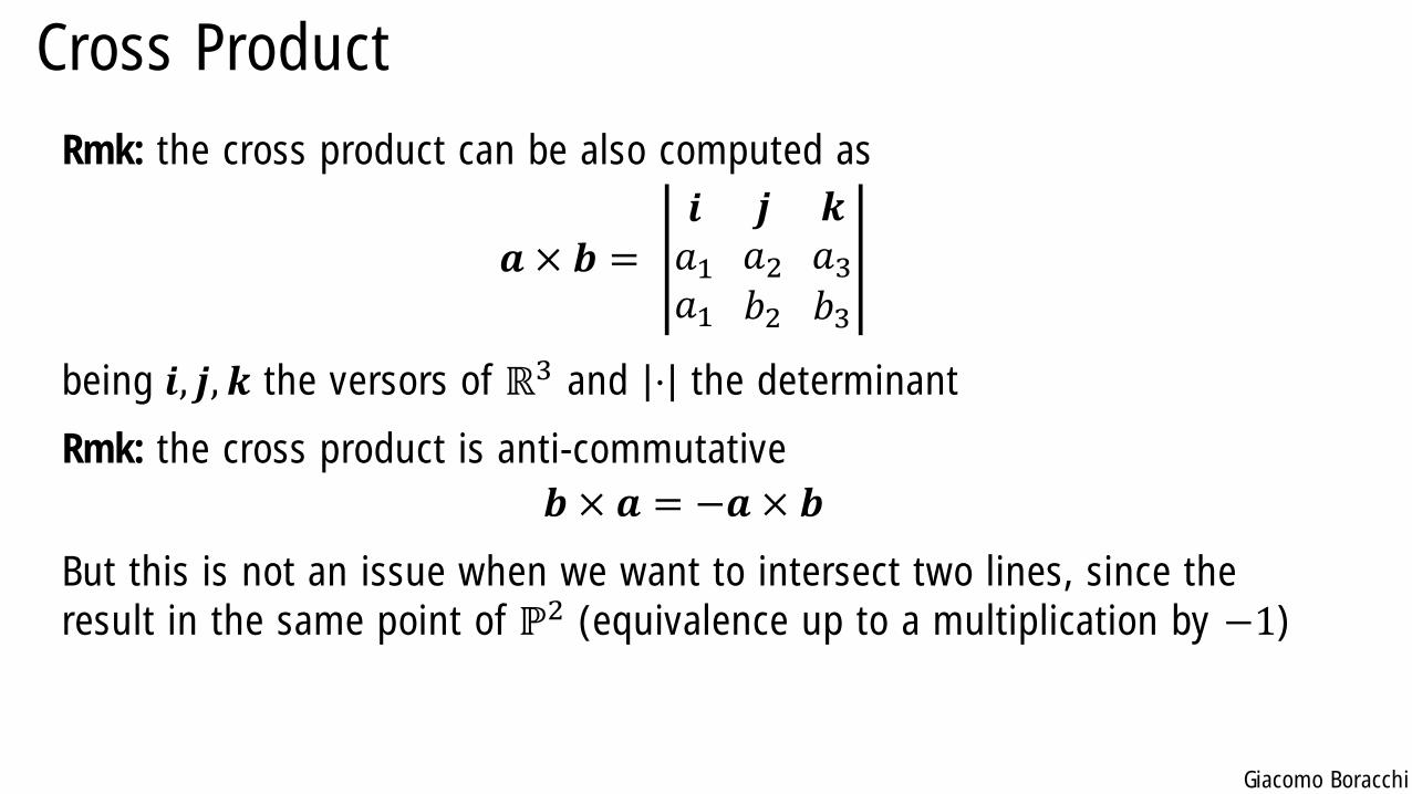
Rmk: the cross product can be also computed as
𝒂 × 𝒃 =𝒊𝑎1𝑎1
𝒋𝑎2𝑏2
𝒌𝑎3𝑏3
being 𝒊, 𝒋, 𝒌 the versors of ℝ3 and ⋅ the determinant
Rmk: the cross product is anti-commutative
𝒃 × 𝒂 = −𝒂 × 𝒃
But this is not an issue when we want to intersect two lines, since the
result in the same point of ℙ2 (equivalence up to a multiplication by −1)
Giacomo Boracchi
Cross Product
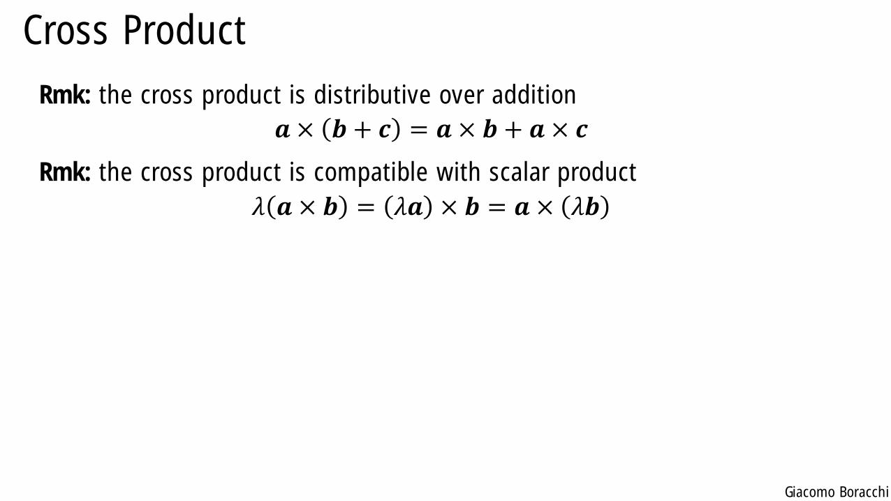
Rmk: the cross product is distributive over addition
𝒂 × 𝒃 + 𝒄 = 𝒂 × 𝒃 + 𝒂 × 𝒄
Rmk: the cross product is compatible with scalar product
𝜆 𝒂 × 𝒃 = 𝜆𝒂 × 𝒃 = 𝒂 × 𝜆𝒃
Giacomo Boracchi
Cross Product
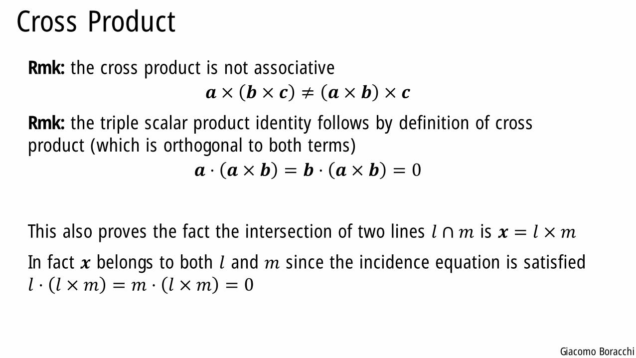
Rmk: the cross product is not associative
𝒂 × 𝒃 × 𝒄 ≠ 𝒂 × 𝒃 × 𝒄
Rmk: the triple scalar product identity follows by definition of cross
product (which is orthogonal to both terms)
𝒂 ⋅ 𝒂 × 𝒃 = 𝒃 ⋅ 𝒂 × 𝒃 = 0
This also proves the fact the intersection of two lines 𝑙 ∩ 𝑚 is 𝒙 = 𝑙 × 𝑚
In fact 𝒙 belongs to both 𝑙 and 𝑚 since the incidence equation is satisfied
𝑙 ⋅ 𝑙 × 𝑚 = 𝑚 ⋅ 𝑙 × 𝑚 = 0
Giacomo Boracchi
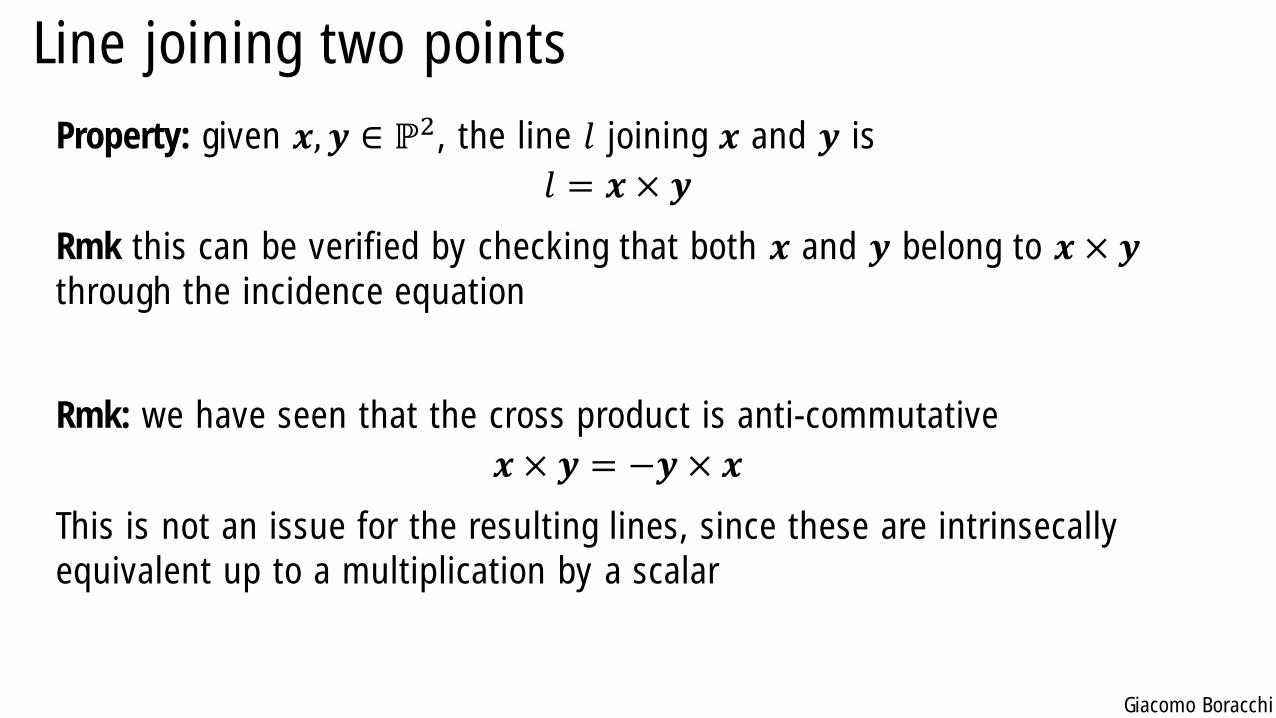
Line joining two points
Property: given 𝒙, 𝒚 ∈ ℙ2, the line 𝑙 joining 𝒙 and 𝒚 is
𝑙 = 𝒙 × 𝒚
Rmk this can be verified by checking that both 𝒙 and 𝒚 belong to 𝒙 × 𝒚through the incidence equation
Rmk: we have seen that the cross product is anti-commutative
𝒙 × 𝒚 = −𝒚 × 𝒙
This is not an issue for the resulting lines, since these are intrinsecally
equivalent up to a multiplication by a scalar
Giacomo Boracchi
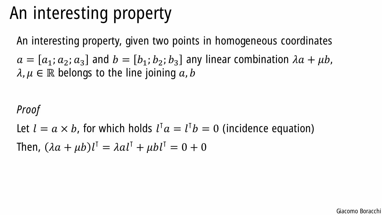
An interesting property
An interesting property, given two points in homogeneous coordinates
𝑎 = 𝑎1; 𝑎2; 𝑎3 and 𝑏 = 𝑏1; 𝑏2; 𝑏3 any linear combination 𝜆𝑎 + 𝜇𝑏,𝜆, 𝜇 ∈ ℝ belongs to the line joining 𝑎, 𝑏
Proof
Let 𝑙 = 𝑎 × 𝑏, for which holds 𝑙⊺𝑎 = 𝑙⊺𝑏 = 0 (incidence equation)
Then, 𝜆𝑎 + 𝜇𝑏 𝑙⊺ = 𝜆𝑎𝑙⊺ + 𝜇𝑏𝑙⊺ = 0 + 0
Giacomo Boracchi
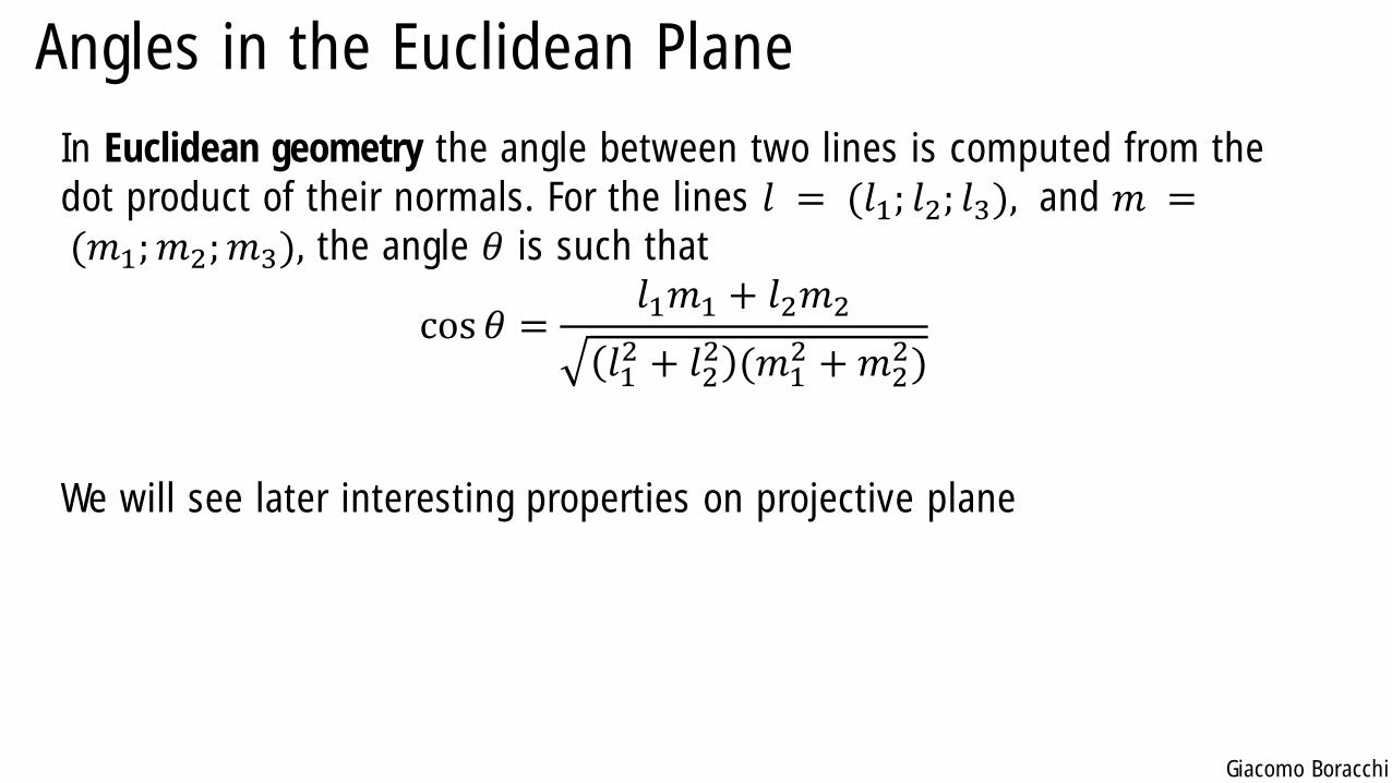
Angles in the Euclidean Plane
In Euclidean geometry the angle between two lines is computed from the
dot product of their normals. For the lines 𝑙 = (𝑙1; 𝑙2; 𝑙3), and 𝑚 =(𝑚1;𝑚2;𝑚3), the angle 𝜃 is such that
cos 𝜃 =𝑙1𝑚1 + 𝑙2𝑚2
𝑙12 + 𝑙2
2 (𝑚12 +𝑚2
2)
We will see later interesting properties on projective plane
Giacomo Boracchi
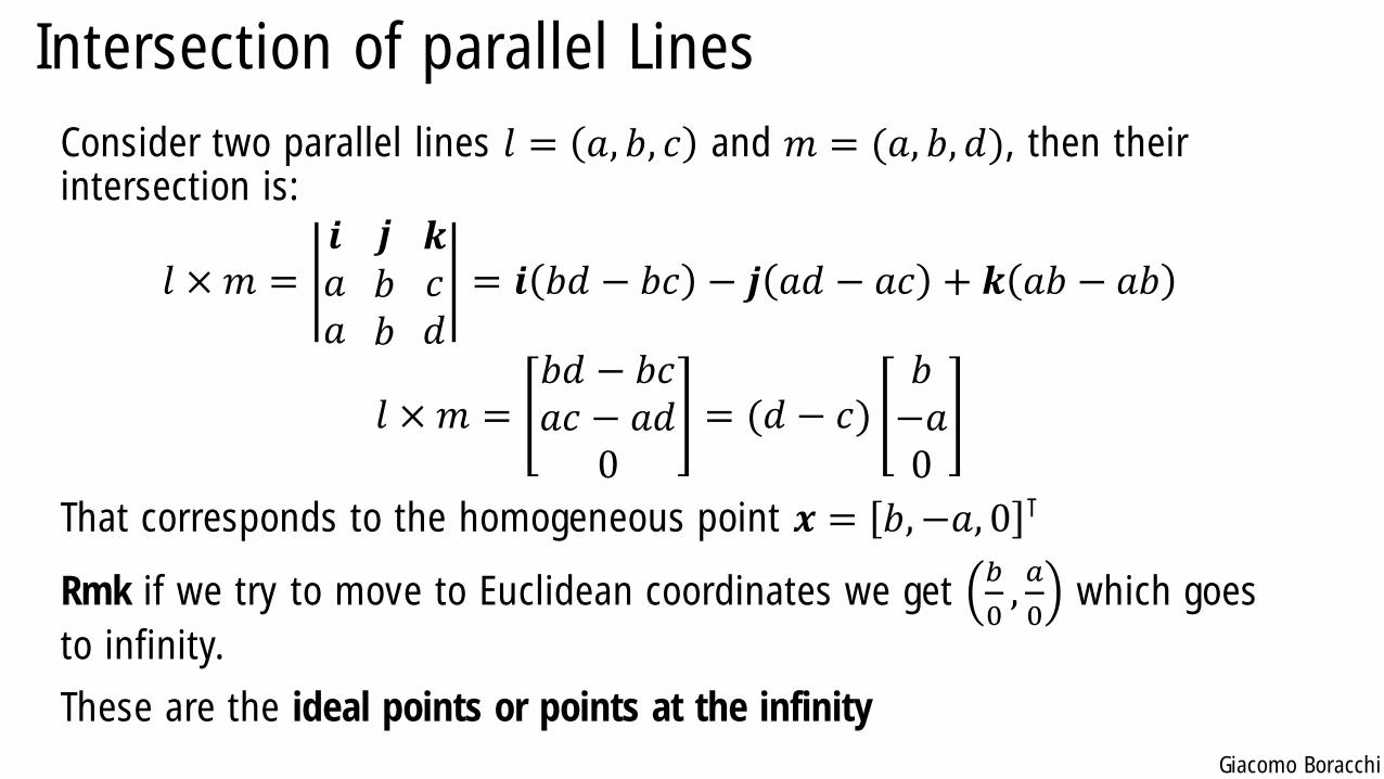
Intersection of parallel Lines
Consider two parallel lines 𝑙 = 𝑎, 𝑏, 𝑐 and 𝑚 = (𝑎, 𝑏, 𝑑), then their intersection is:
𝑙 × 𝑚 =𝒊𝑎𝑎
𝒋𝑏𝑏
𝒌𝑐𝑑
= 𝒊 𝑏𝑑 − 𝑏𝑐 − 𝒋 𝑎𝑑 − 𝑎𝑐 + 𝒌 𝑎𝑏 − 𝑎𝑏
𝑙 × 𝑚 =𝑏𝑑 − 𝑏𝑐𝑎𝑐 − 𝑎𝑑
0= (𝑑 − 𝑐)
𝑏−𝑎0
That corresponds to the homogeneous point 𝒙 = 𝑏,−𝑎, 0 ⊺
Rmk if we try to move to Euclidean coordinates we get 𝑏
0,𝑎
0which goes
to infinity.
These are the ideal points or points at the infinity
Giacomo Boracchi
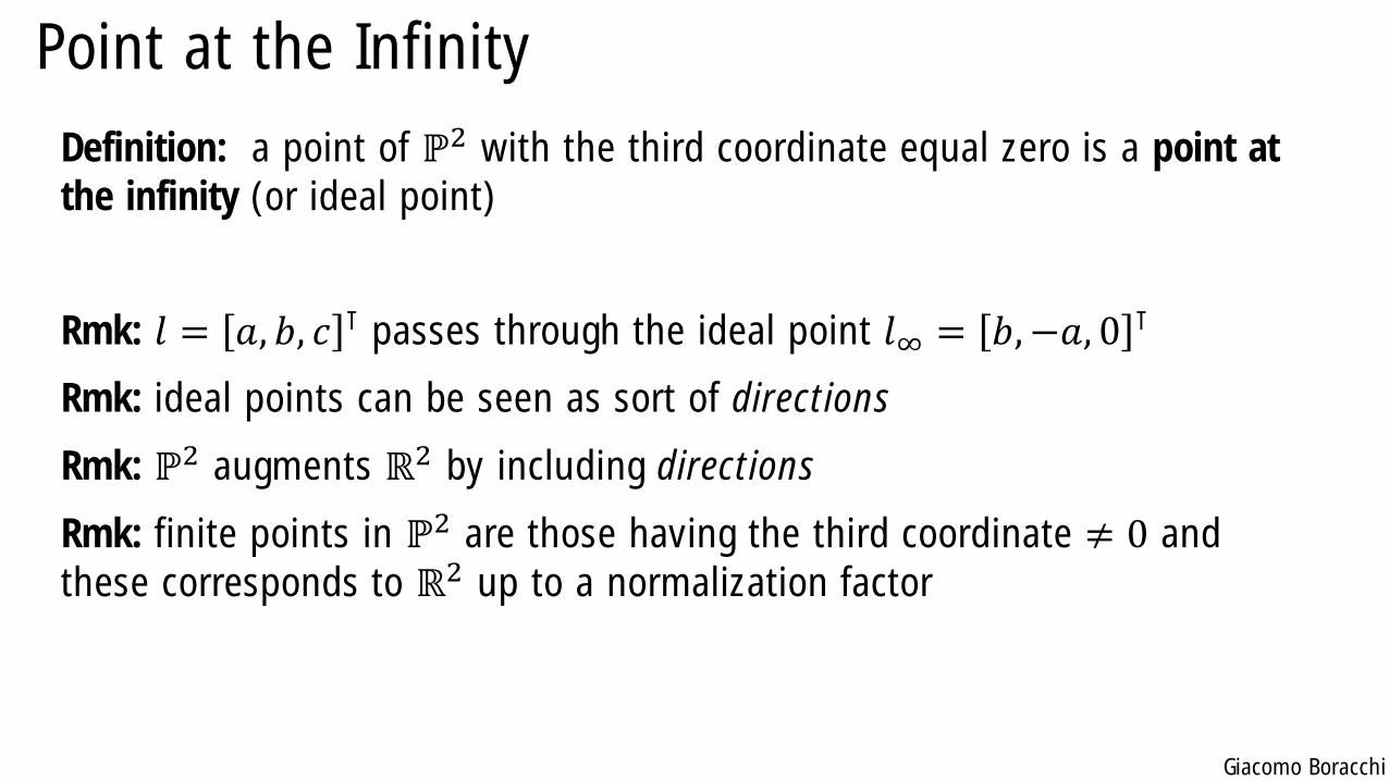
Point at the Infinity
Definition: a point of ℙ2 with the third coordinate equal zero is a point at
the infinity (or ideal point)
Rmk: 𝑙 = 𝑎, 𝑏, 𝑐 ⊺ passes through the ideal point 𝑙∞ = 𝑏,−𝑎, 0 ⊺
Rmk: ideal points can be seen as sort of directions
Rmk: ℙ2 augments ℝ2 by including directions
Rmk: finite points in ℙ2 are those having the third coordinate ≠ 0 and
these corresponds to ℝ2 up to a normalization factor
Giacomo Boracchi
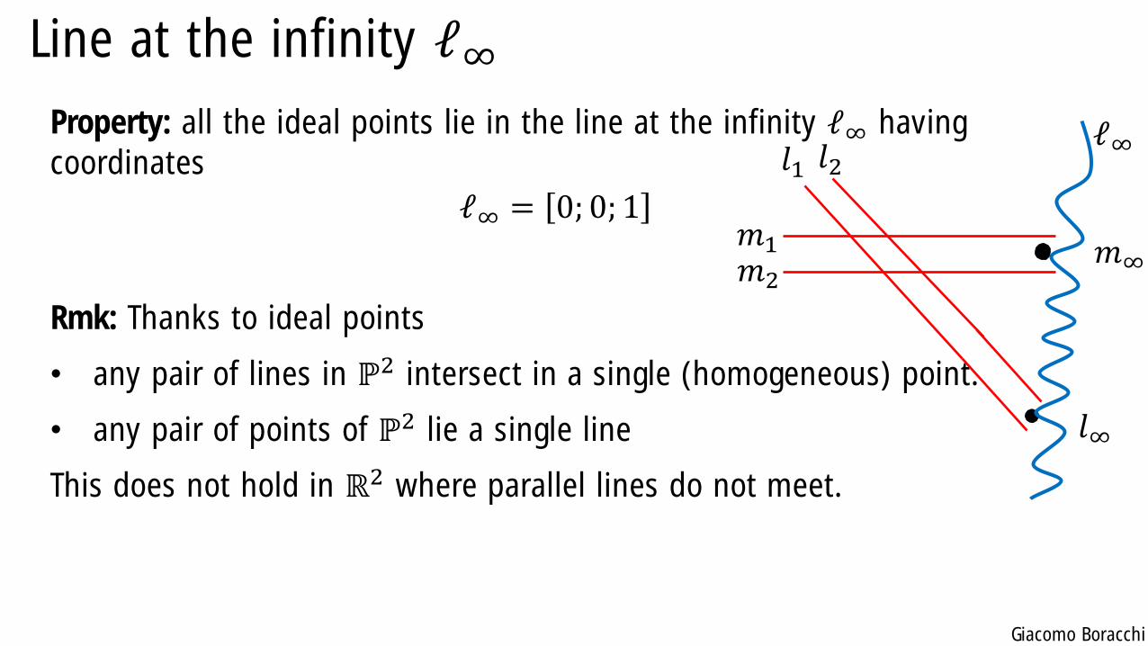
Line at the infinity ℓ∞
Property: all the ideal points lie in the line at the infinity ℓ∞ having
coordinates
ℓ∞ = 0; 0; 1
Rmk: Thanks to ideal points
• any pair of lines in ℙ2 intersect in a single (homogeneous) point.
• any pair of points of ℙ2 lie a single line
This does not hold in ℝ2 where parallel lines do not meet.
ℓ∞𝑙1 𝑙2
𝑚∞𝑚1𝑚2
𝑙∞
Giacomo Boracchi
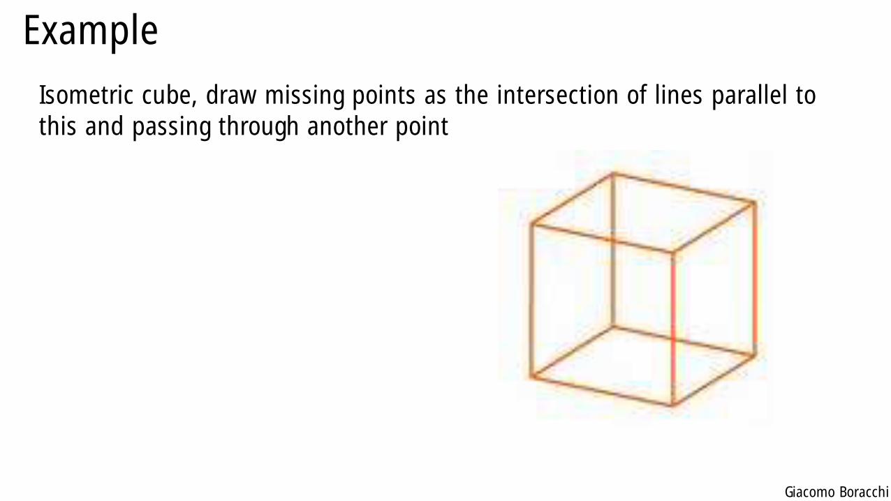
Example
Isometric cube, draw missing points as the intersection of lines parallel to
this and passing through another point
Giacomo Boracchi
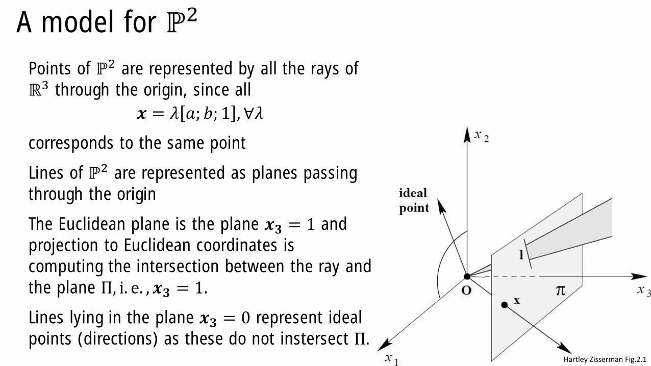
A model for ℙ2
Points of ℙ2 are represented by all the rays of
ℝ3 through the origin, since all
𝒙 = 𝜆 𝑎; 𝑏; 1 , ∀𝜆
corresponds to the same point
Lines of ℙ2 are represented as planes passing
through the origin
The Euclidean plane is the plane 𝒙𝟑 = 1 and
projection to Euclidean coordinates is
computing the intersection between the ray and
the plane Π, i. e. , 𝒙𝟑 = 1.
Lines lying in the plane 𝒙𝟑 = 0 represent ideal
points (directions) as these do not instersect Π.Hartley Zisserman Fig.2.1
Giacomo Boracchi
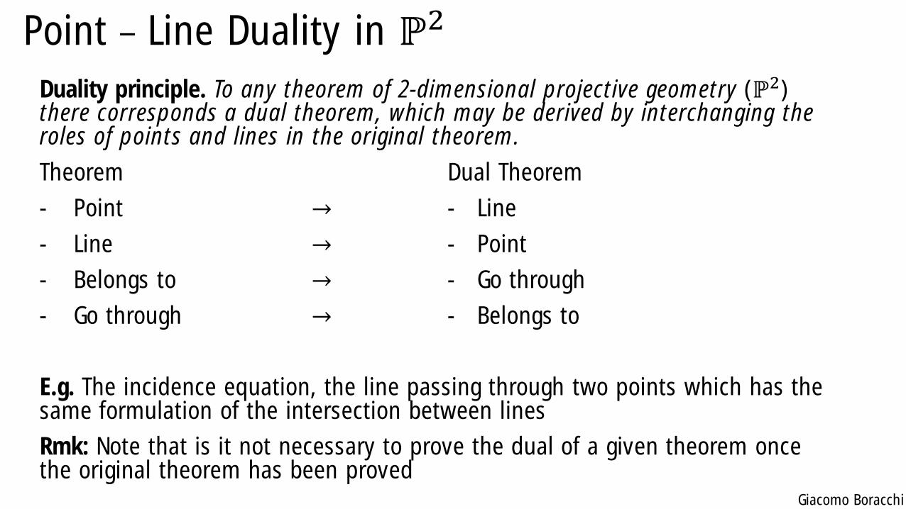
Point Line Duality in ℙ2
Duality principle. To any theorem of 2-dimensional projective geometry (ℙ2)there corresponds a dual theorem, which may be derived by interchanging the roles of points and lines in the original theorem.
Theorem Dual Theorem
- Point → - Line
- Line → - Point
- Belongs to → - Go through
- Go through → - Belongs to
E.g. The incidence equation, the line passing through two points which has the same formulation of the intersection between lines
Rmk: Note that is it not necessary to prove the dual of a given theorem once the original theorem has been proved
Giacomo Boracchi
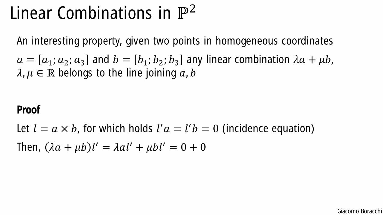
Linear Combinations in ℙ2
An interesting property, given two points in homogeneous coordinates
𝑎 = 𝑎1; 𝑎2; 𝑎3 and 𝑏 = 𝑏1; 𝑏2; 𝑏3 any linear combination 𝜆𝑎 + 𝜇𝑏,𝜆, 𝜇 ∈ ℝ belongs to the line joining 𝑎, 𝑏
Proof
Let 𝑙 = 𝑎 × 𝑏, for which holds 𝑙′𝑎 = 𝑙′𝑏 = 0 (incidence equation)
Then, 𝜆𝑎 + 𝜇𝑏 𝑙′ = 𝜆𝑎𝑙′ + 𝜇𝑏𝑙′ = 0 + 0

Giacomo Boracchi
Single-View GeometryGiacomo Boracchi
February 28th, 2020
USI, Lugano
Book: HZ, chapter 4
Giacomo Boracchi
Outline
• Trasformations in ℙ2
• The Projective Space ℙ3
• Vanishing Points
• Affine Rectification
Giacomo Boracchi
Transformations in ℙ2
Giacomo Boracchi
Homographies
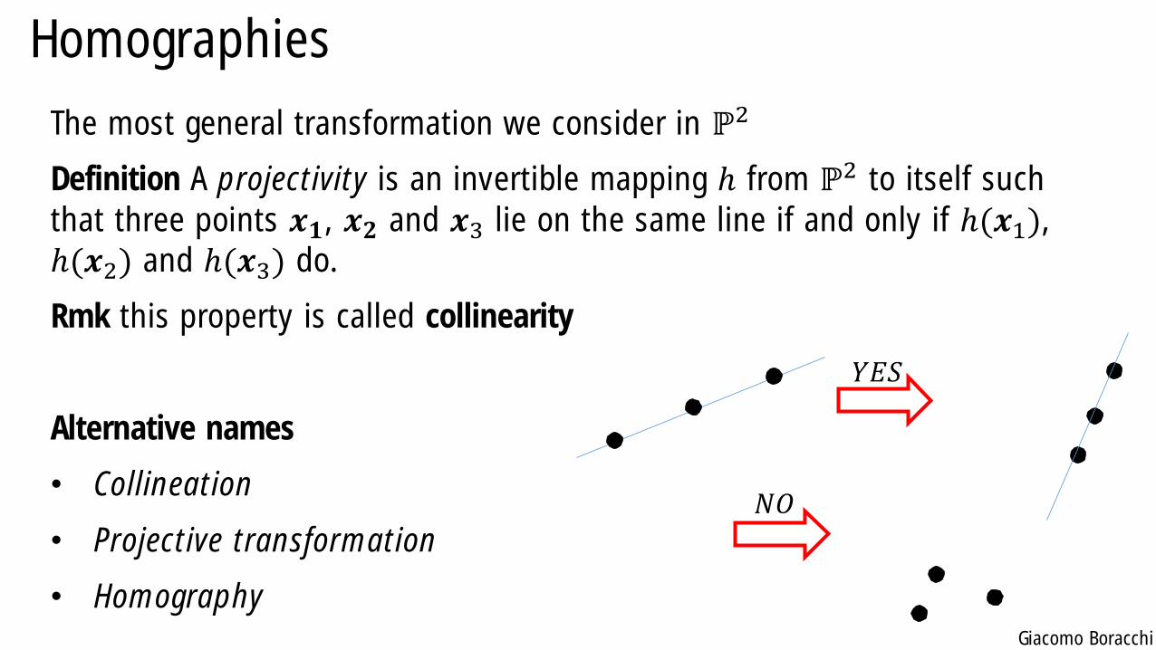
The most general transformation we consider in ℙ2
Definition A projectivity is an invertible mapping ℎ from ℙ2 to itself such
that three points 𝒙𝟏, 𝒙𝟐 and 𝒙3 lie on the same line if and only if ℎ(𝒙1), ℎ(𝒙2) and ℎ(𝒙3) do.
Rmk this property is called collinearity
Alternative names
• Collineation
• Projective transformation
• Homography
𝑌𝐸𝑆
𝑁𝑂
Giacomo Boracchi
Homographies
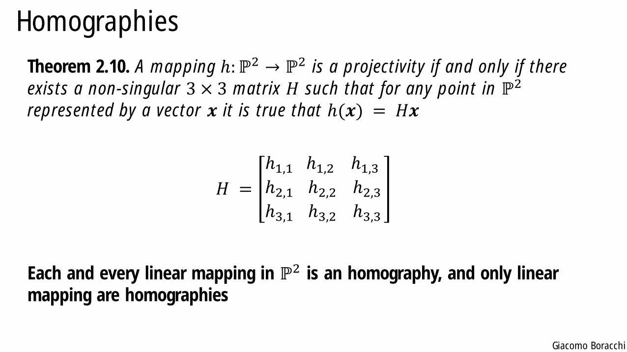
Theorem 2.10. A mapping ℎ:ℙ2 → ℙ2 is a projectivity if and only if there
exists a non-singular 3 × 3 matrix 𝐻 such that for any point in ℙ2
represented by a vector 𝒙 it is true that ℎ(𝒙) = 𝐻𝒙
𝐻 =
ℎ1,1ℎ2,1ℎ3,1
ℎ1,2ℎ2,2ℎ3,2
ℎ1,3ℎ2,3ℎ3,3
Each and every linear mapping in ℙ2 is an homography, and only linear
mapping are homographies
Giacomo Boracchi
Homographies and Points in ℙ2
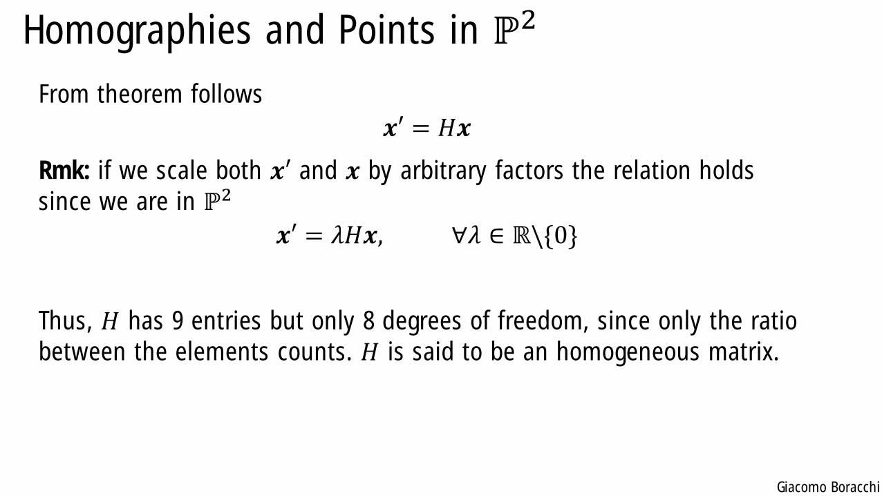
From theorem follows
𝒙′ = 𝐻𝒙
Rmk: if we scale both 𝒙′ and 𝒙 by arbitrary factors the relation holds
since we are in ℙ2
𝒙′ = 𝜆𝐻𝒙, ∀𝜆 ∈ ℝ\{0}
Thus, 𝐻 has 9 entries but only 8 degrees of freedom, since only the ratio
between the elements counts. 𝐻 is said to be an homogeneous matrix.
Giacomo Boracchi
Homographies and Lines in ℙ2
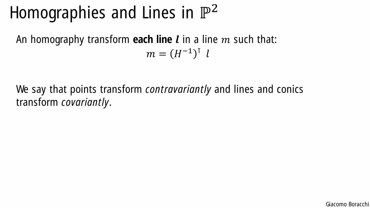
An homography transform each line 𝒍 in a line 𝑚 such that:
𝑚 = 𝐻−1 ⊺ 𝑙
We say that points transform contravariantly and lines and conics
transform covariantly.
Giacomo Boracchi
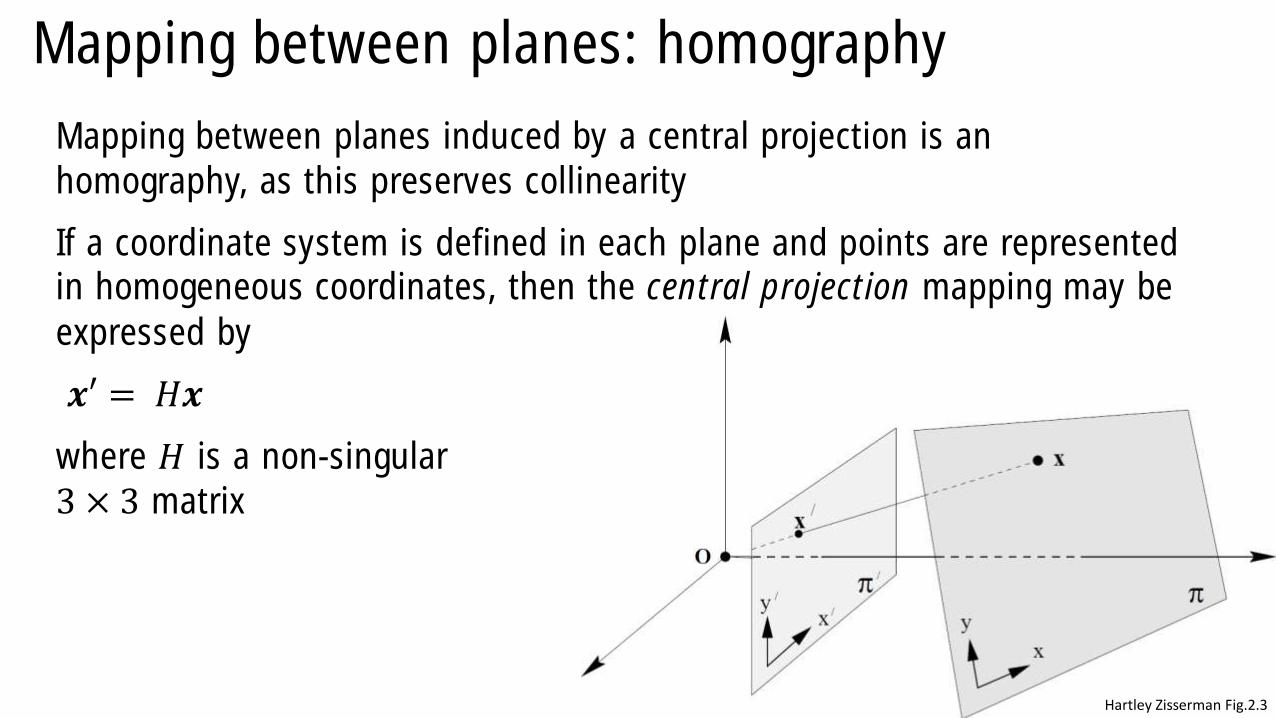
Mapping between planes: homography
Mapping between planes induced by a central projection is an
homography, as this preserves collinearity
If a coordinate system is defined in each plane and points are represented
in homogeneous coordinates, then the central projection mapping may be
expressed by
𝒙′ = 𝐻𝒙
where 𝐻 is a non-singular
3 × 3 matrix
Hartley Zisserman Fig.2.3
Giacomo Boracchi
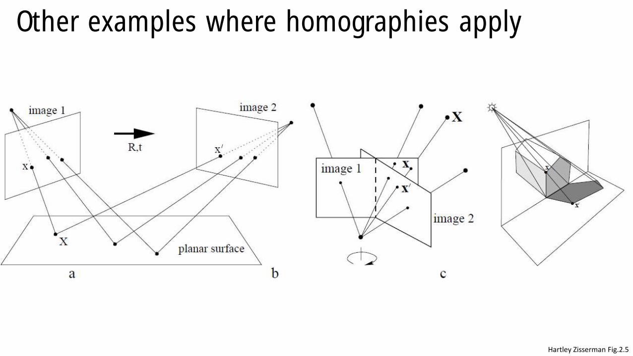
Other examples where homographies apply
Hartley Zisserman Fig.2.5

Giacomo Boracchi
A Hierarchy of Transformations
Giacomo Boracchi
Linear Transformation
We consider linear transformations of ℙ2,
• these can be expressed as a 3 × 3 matrix 𝐻,
• the homogeneous constraint applies
Depending on the structure of 𝐻 there are different class of
transformations with a different number of degrees of freedom
Giacomo Boracchi
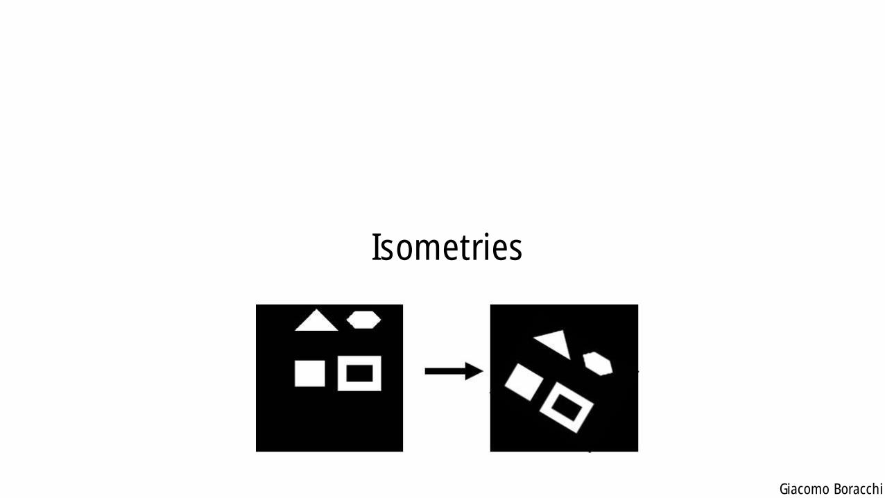
Isometries
Giacomo Boracchi
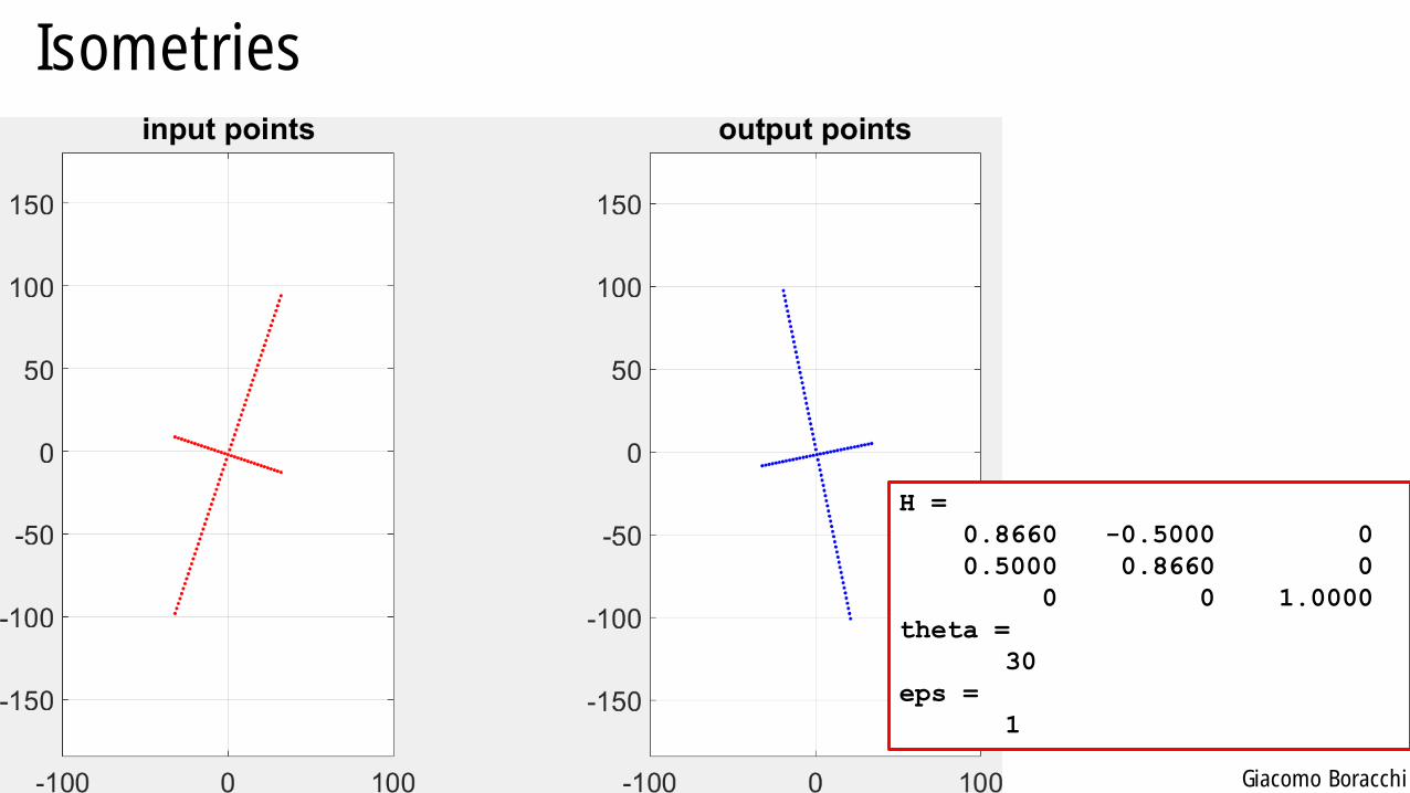
Isometries
H =
0.8660 -0.5000 0
0.5000 0.8660 0
0 0 1.0000
theta =
30
eps =
1
Giacomo Boracchi
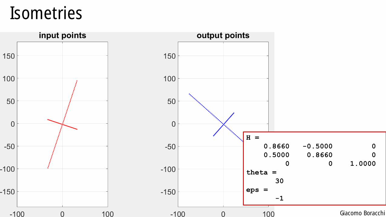
Isometries
H =
0.8660 -0.5000 0
0.5000 0.8660 0
0 0 1.0000
theta =
30
eps =
-1
Giacomo Boracchi
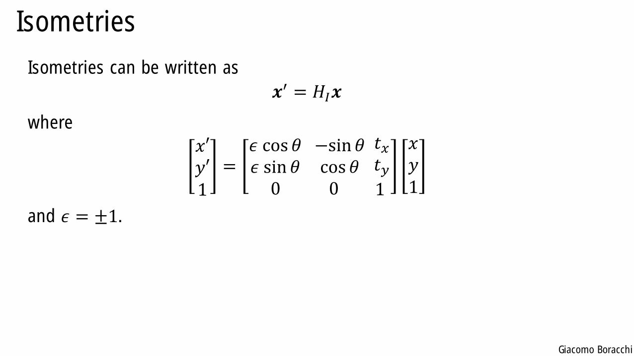
Isometries
Isometries can be written as
𝒙′ = 𝐻𝐼𝒙
where
𝑥′𝑦′1
=𝜖 cos 𝜃𝜖 sin 𝜃0
−sin𝜃cos 𝜃0
𝑡𝑥𝑡𝑦1
𝑥𝑦1
and 𝜖 = ±1.
Giacomo Boracchi
Isometries
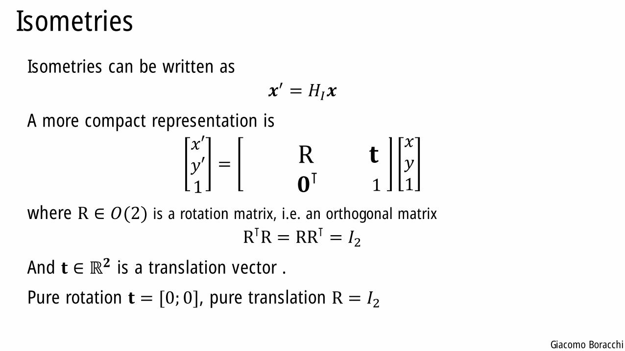
Isometries can be written as
𝒙′ = 𝐻𝐼𝒙
A more compact representation is
𝑥′𝑦′1
=𝜖 cos 𝜃𝜖 sin 𝜃0
− sin 𝜃cos 𝜃0
𝑡𝑥
1
𝑥𝑦1
where R ∈ 𝑂(2) is a rotation matrix, i.e. an orthogonal matrix
R⊺R = RR⊺ = 𝐼2
And 𝐭 ∈ ℝ𝟐 is a translation vector .
Pure rotation 𝐭 = [0; 0], pure translation R = 𝐼2
R 𝐭𝟎⊺
Giacomo Boracchi
Isometries: Invariants
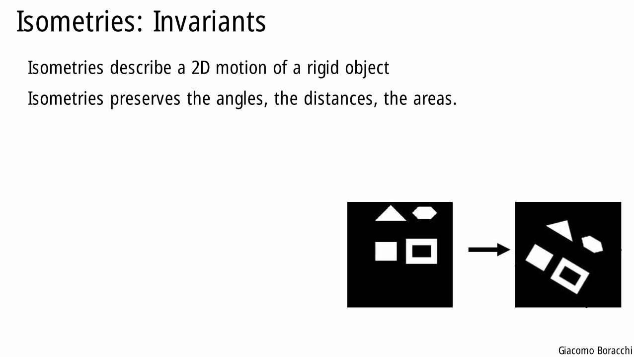
Isometries describe a 2D motion of a rigid object
Isometries preserves the angles, the distances, the areas.
Giacomo Boracchi
Isometries: Remarks
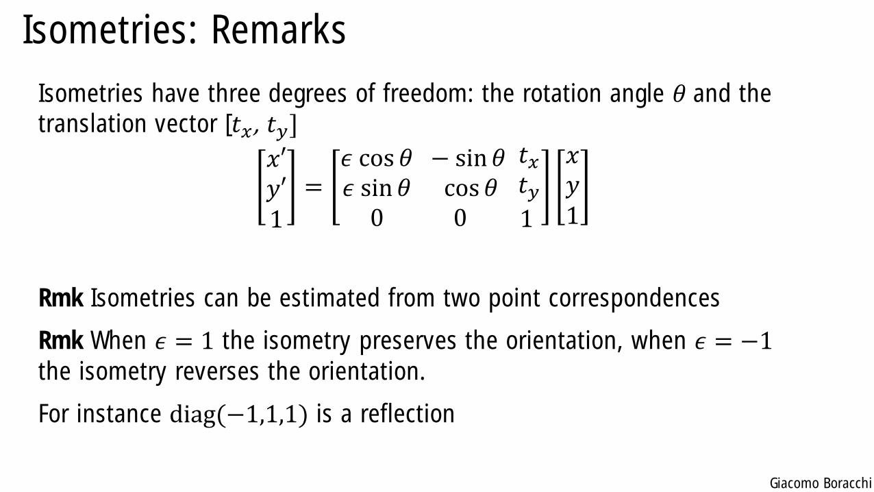
Isometries have three degrees of freedom: the rotation angle 𝜃 and the
translation vector [𝑡𝑥 , 𝑡𝑦]
𝑥′𝑦′1
=𝜖 cos 𝜃𝜖 sin 𝜃0
− sin𝜃cos 𝜃0
𝑡𝑥𝑡𝑦1
𝑥𝑦1
Rmk Isometries can be estimated from two point correspondences
Rmk When 𝜖 = 1 the isometry preserves the orientation, when 𝜖 = −1the isometry reverses the orientation.
For instance diag(−1,1,1) is a reflection
Giacomo Boracchi
Isometries: Remarks
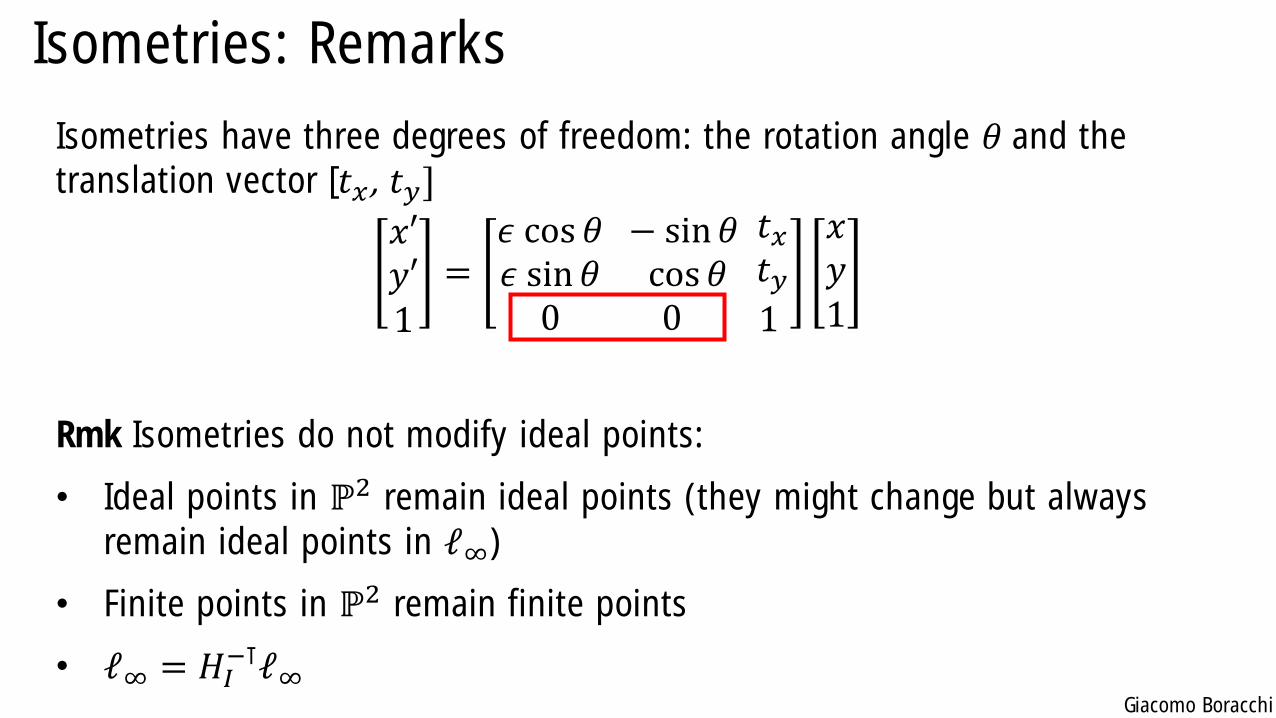
Isometries have three degrees of freedom: the rotation angle 𝜃 and the
translation vector [𝑡𝑥 , 𝑡𝑦]
𝑥′𝑦′1
=𝜖 cos 𝜃𝜖 sin 𝜃0
− sin𝜃cos 𝜃0
𝑡𝑥𝑡𝑦1
𝑥𝑦1
Rmk Isometries do not modify ideal points:
• Ideal points in ℙ2 remain ideal points (they might change but always
remain ideal points in ℓ∞)
• Finite points in ℙ2 remain finite points
• ℓ∞ = 𝐻𝐼−⊺ℓ∞
Giacomo Boracchi
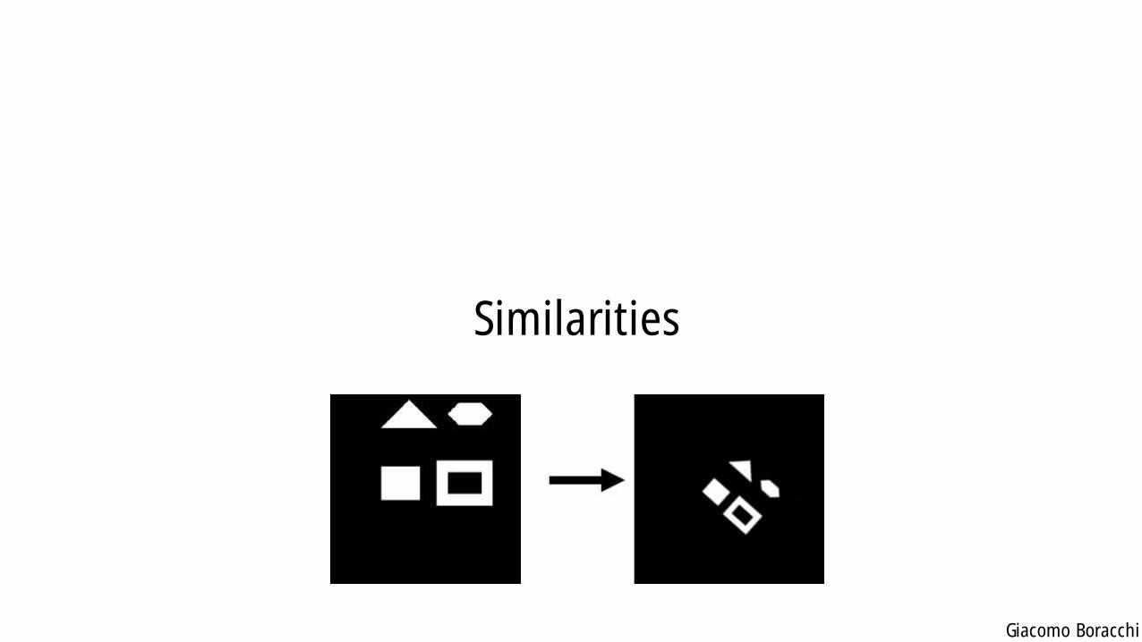
Similarities
Giacomo Boracchi
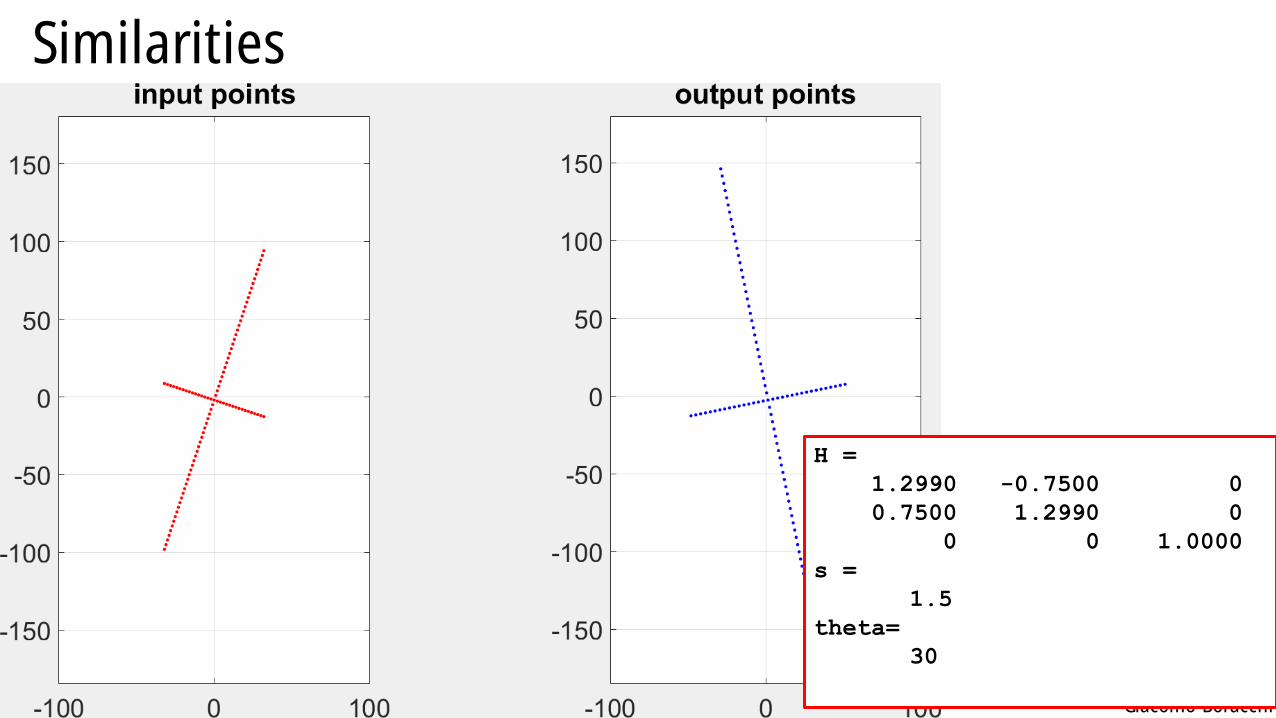
Similarities
H =
1.2990 -0.7500 0
0.7500 1.2990 0
0 0 1.0000
s =
1.5
theta=
30
Giacomo Boracchi
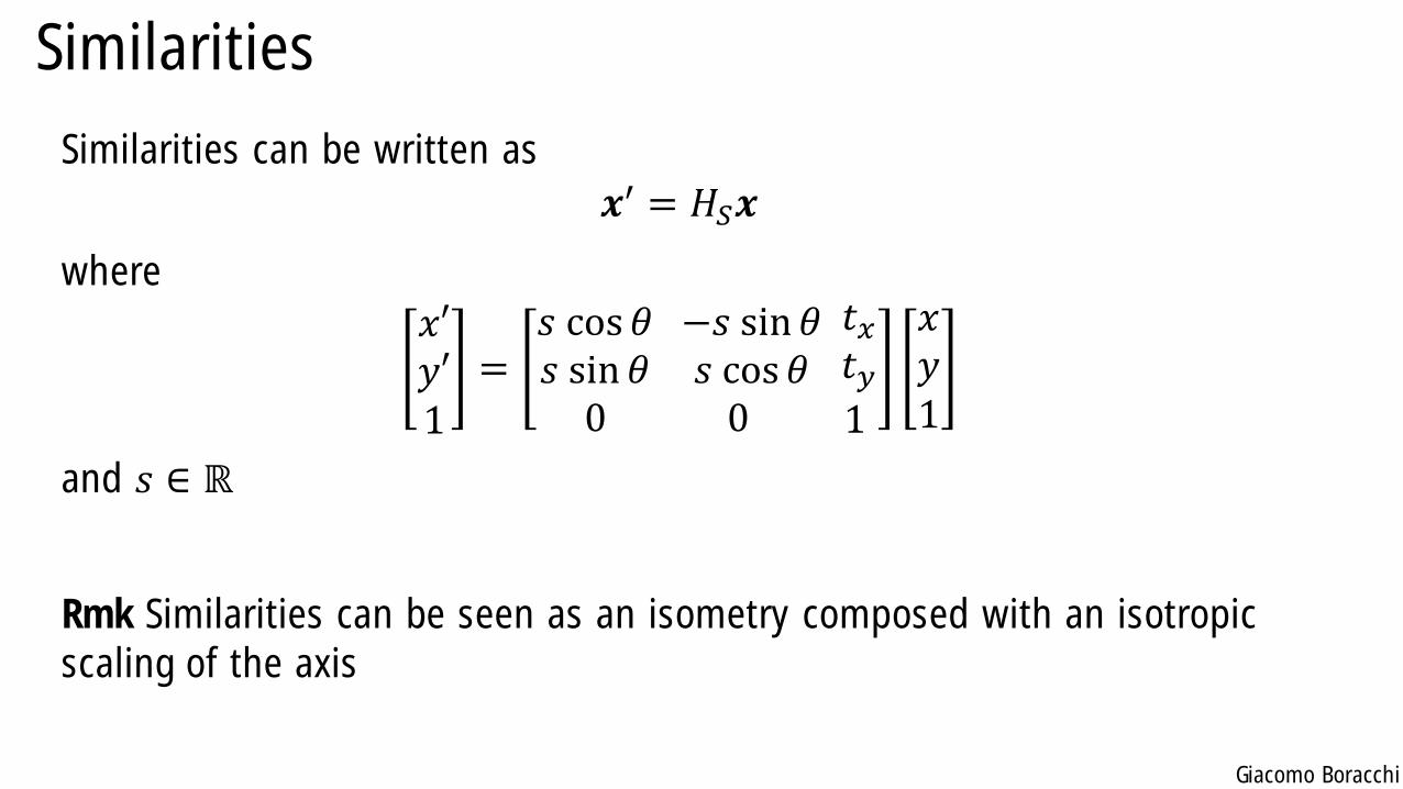
Similarities
Similarities can be written as
𝒙′ = 𝐻𝑆𝒙
where
𝑥′𝑦′1
=𝑠 cos 𝜃𝑠 sin 𝜃0
−𝑠 sin 𝜃𝑠 cos 𝜃0
𝑡𝑥𝑡𝑦1
𝑥𝑦1
and 𝑠 ∈ ℝ
Rmk Similarities can be seen as an isometry composed with an isotropic
scaling of the axis
Giacomo Boracchi
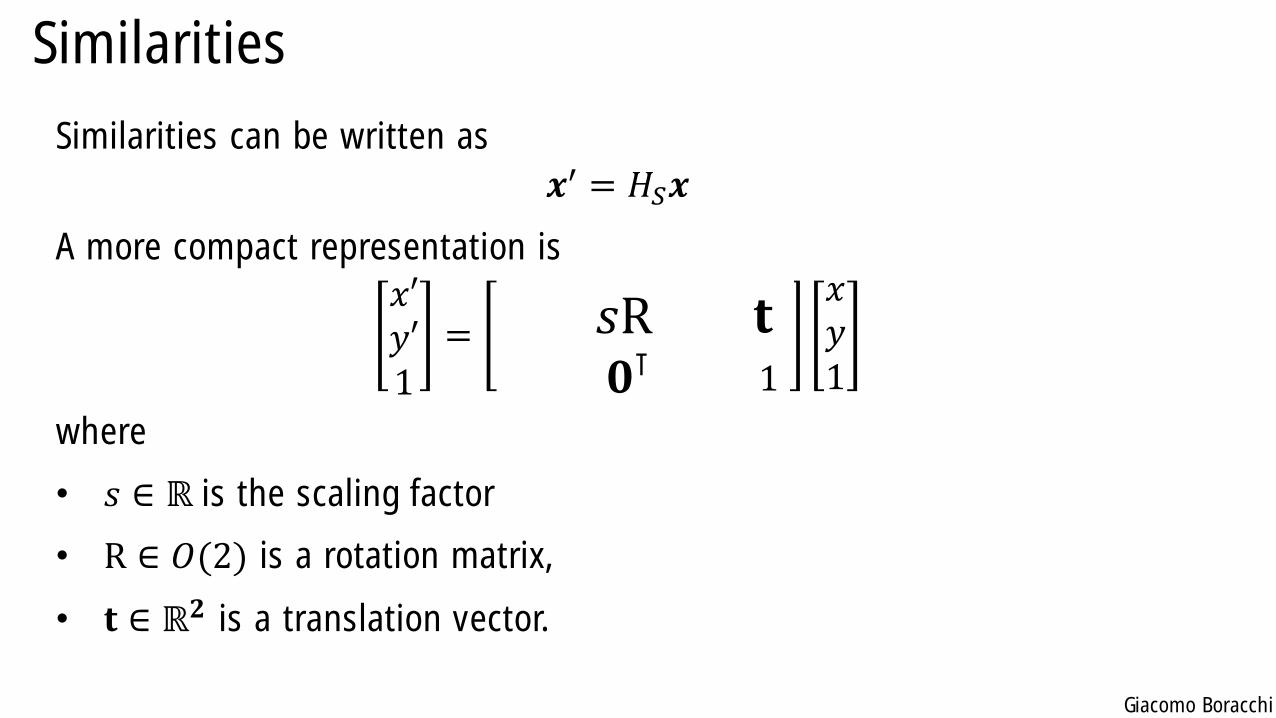
Similarities
Similarities can be written as
𝒙′ = 𝐻𝑆𝒙
A more compact representation is
𝑥′𝑦′1
=𝜖 cos 𝜃𝜖 sin 𝜃0
− sin 𝜃cos 𝜃0
𝑡𝑥
1
𝑥𝑦1
where
• 𝑠 ∈ ℝ is the scaling factor
• R ∈ 𝑂(2) is a rotation matrix,
• 𝐭 ∈ ℝ𝟐 is a translation vector.
𝑠R 𝐭𝟎⊺
Giacomo Boracchi
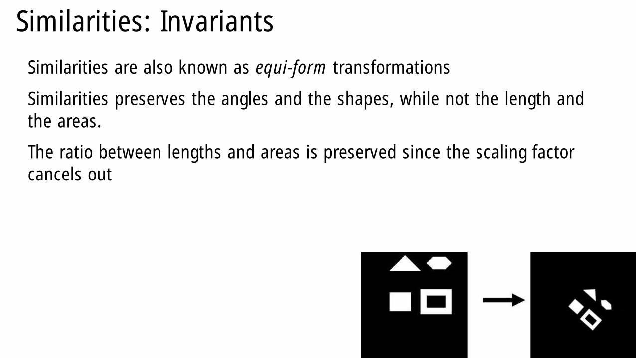
Similarities: Invariants
Similarities are also known as equi-form transformations
Similarities preserves the angles and the shapes, while not the length and
the areas.
The ratio between lengths and areas is preserved since the scaling factor
cancels out
Giacomo Boracchi
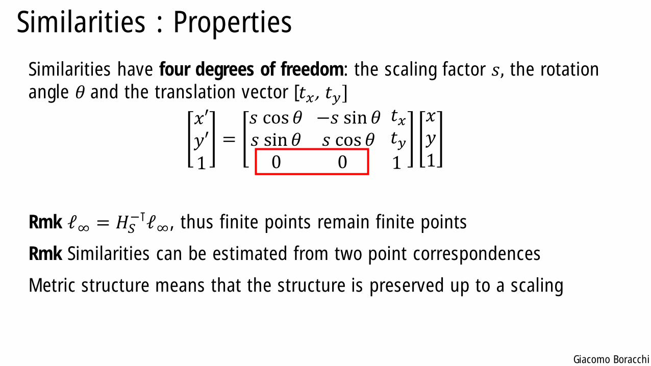
Similarities : Properties
Similarities have four degrees of freedom: the scaling factor 𝑠, the rotation
angle 𝜃 and the translation vector [𝑡𝑥 , 𝑡𝑦]
𝑥′𝑦′1
=𝑠 cos 𝜃𝑠 sin 𝜃0
−𝑠 sin 𝜃𝑠 cos 𝜃0
𝑡𝑥𝑡𝑦1
𝑥𝑦1
Rmk ℓ∞ = 𝐻𝑆−⊺ℓ∞, thus finite points remain finite points
Rmk Similarities can be estimated from two point correspondences
Metric structure means that the structure is preserved up to a scaling
Giacomo Boracchi
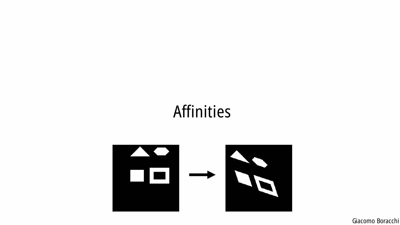
Affinities
Giacomo Boracchi
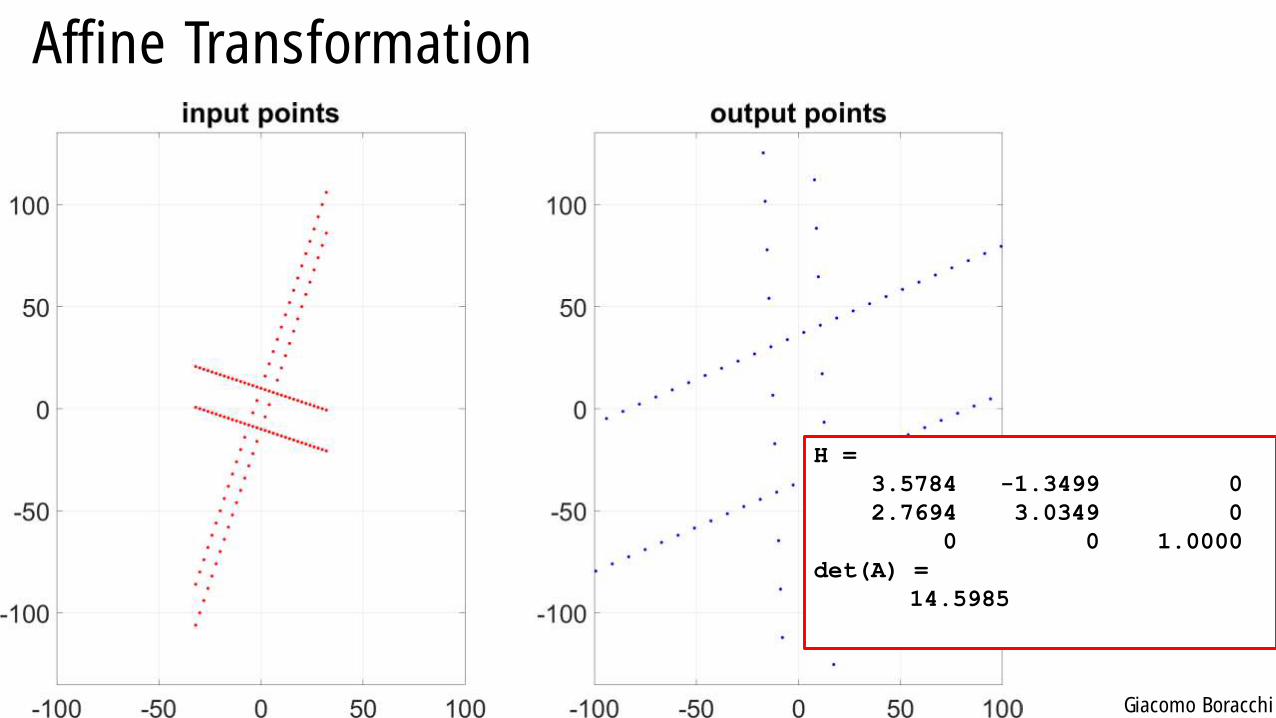
Affine Transformation
H =
3.5784 -1.3499 0
2.7694 3.0349 0
0 0 1.0000
det(A) =
14.5985
Giacomo Boracchi
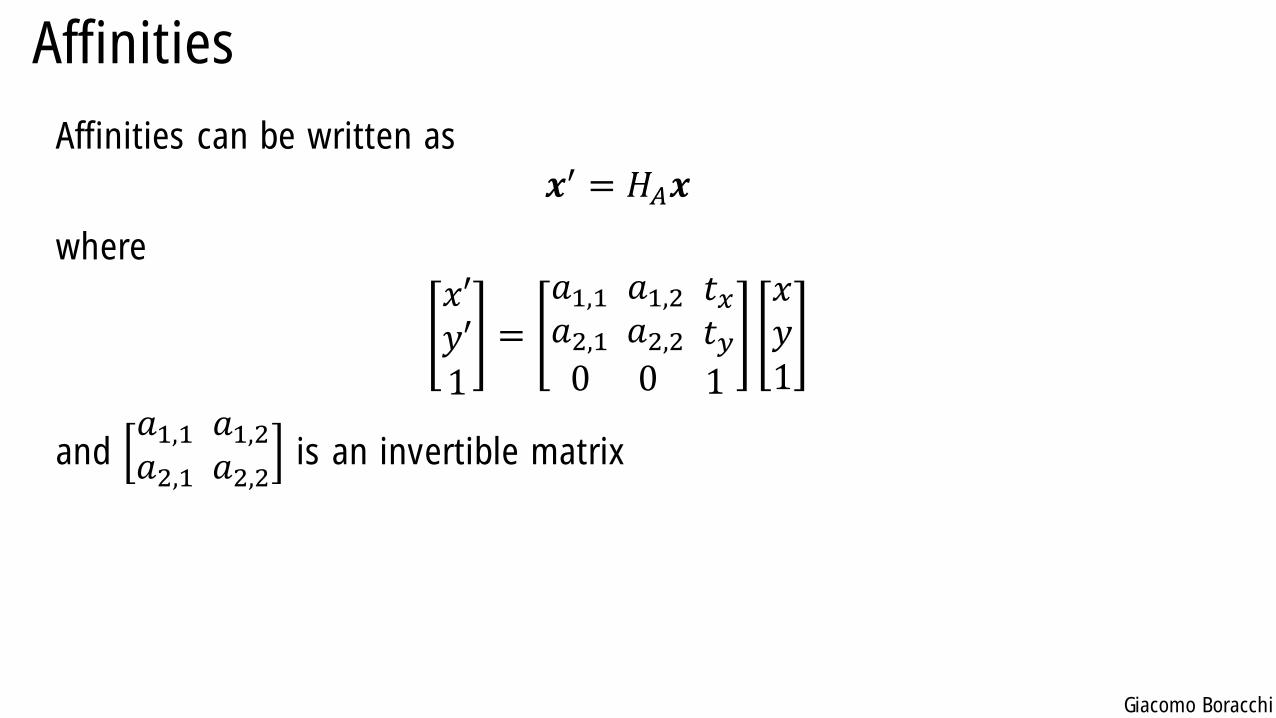
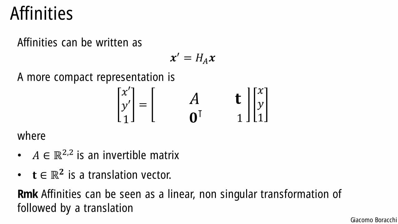
Affinities
Affinities can be written as
𝒙′ = 𝐻𝐴𝒙
where
𝑥′𝑦′1
=
𝑎1,1𝑎2,10
𝑎1,2𝑎2,20
𝑡𝑥𝑡𝑦1
𝑥𝑦1
and 𝑎1,1𝑎2,1
𝑎1,2𝑎2,2
is an invertible matrix
Giacomo Boracchi
Affinities
Affinities can be written as
𝒙′ = 𝐻𝐴𝒙
A more compact representation is
𝑥′𝑦′1
=𝜖 cos 𝜃𝜖 sin 𝜃0
− sin 𝜃cos 𝜃0
𝑡𝑥
1
𝑥𝑦1
where
• 𝐴 ∈ ℝ2,2 is an invertible matrix
• 𝐭 ∈ ℝ𝟐 is a translation vector.
Rmk Affinities can be seen as a linear, non singular transformation of
followed by a translation
𝐴 𝐭𝟎⊺
Giacomo Boracchi
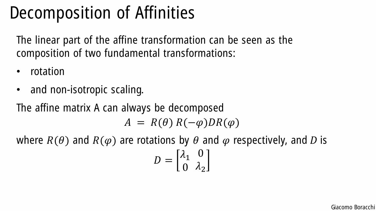
Decomposition of Affinities
The linear part of the affine transformation can be seen as the
composition of two fundamental transformations:
• rotation
• and non-isotropic scaling.
The affine matrix A can always be decomposed
𝐴 = 𝑅(𝜃) 𝑅(−𝜑)𝐷𝑅(𝜑)
where 𝑅(𝜃) and 𝑅(𝜑) are rotations by 𝜃 and 𝜑 respectively, and 𝐷 is
𝐷 =𝜆10
0𝜆2
Giacomo Boracchi
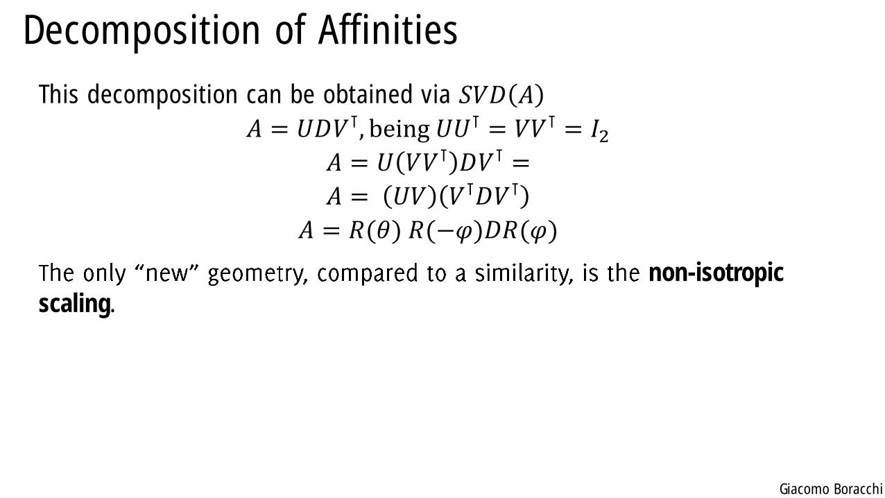
Decomposition of Affinities
This decomposition can be obtained via 𝑆𝑉𝐷 𝐴
𝐴 = 𝑈𝐷𝑉⊺, being 𝑈𝑈⊺ = 𝑉𝑉⊺ = 𝐼2𝐴 = 𝑈 𝑉𝑉⊺ 𝐷𝑉⊺ =
𝐴 = 𝑈𝑉 𝑉⊺𝐷𝑉⊺
𝐴 = 𝑅(𝜃) 𝑅(−𝜑)𝐷𝑅(𝜑)
non-isotropic
scaling.
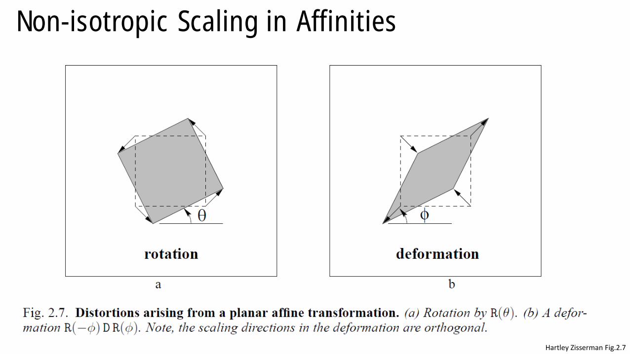
Giacomo Boracchi
Non-isotropic Scaling in Affinities
Hartley Zisserman Fig.2.7

Giacomo Boracchi
Affinities: Invariants
Due to the non-isotropic scaling, the similarity invariants of length ratios
and angles between lines are not preserved under an affinity.
Affinities preserves
• Parallel lines, since ℓ∞ = 𝐻𝐴−⊺ℓ∞
• Ratio of lengths over parallel lines
• Ratio of areas (since each area is scaled of det(𝐴), which cancels out)
Giacomo Boracchi
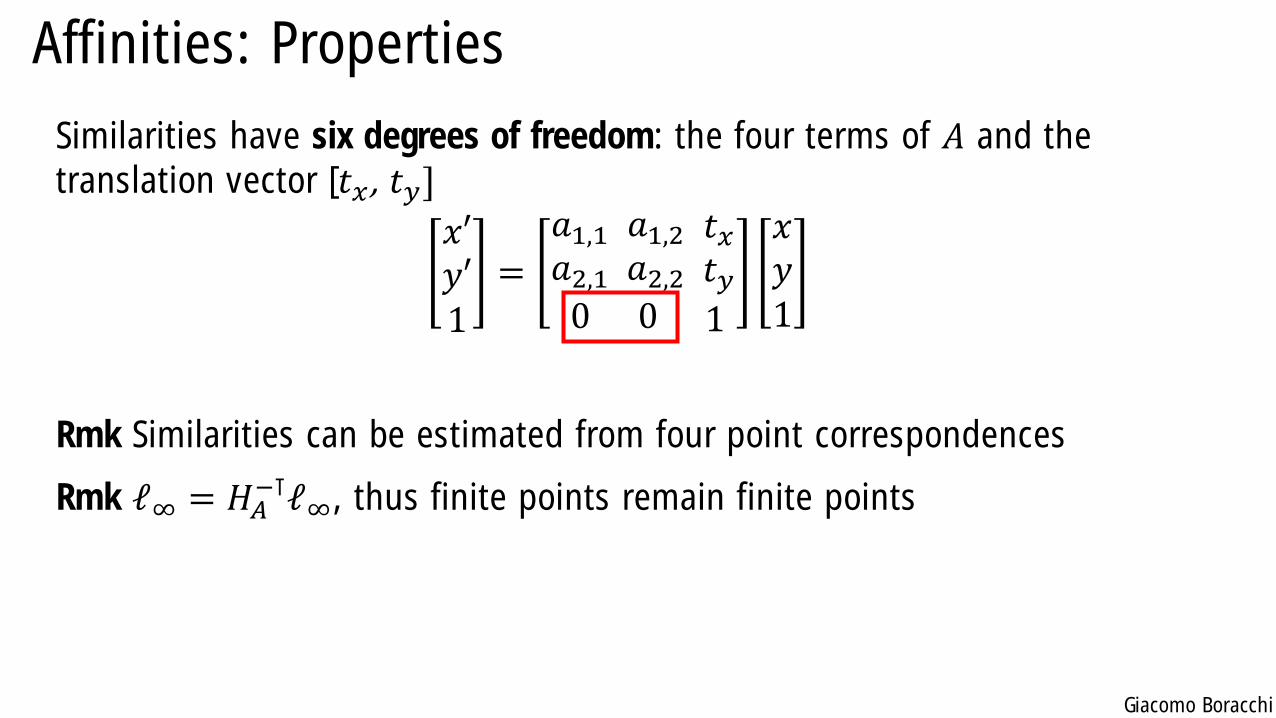
Affinities: Properties
Similarities have six degrees of freedom: the four terms of 𝐴 and the
translation vector [𝑡𝑥 , 𝑡𝑦]
𝑥′𝑦′1
=
𝑎1,1𝑎2,10
𝑎1,2𝑎2,20
𝑡𝑥𝑡𝑦1
𝑥𝑦1
Rmk Similarities can be estimated from four point correspondences
Rmk ℓ∞ = 𝐻𝐴−⊺ℓ∞, thus finite points remain finite points
Giacomo Boracchi
Homographies
Giacomo Boracchi
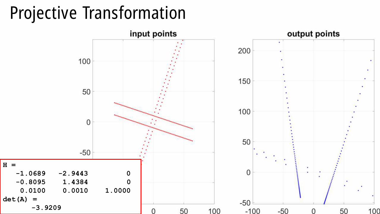
Projective Transformation
H =
-1.0689 -2.9443 0
-0.8095 1.4384 0
0.0100 0.0010 1.0000
det(A) =
-3.9209
Giacomo Boracchi
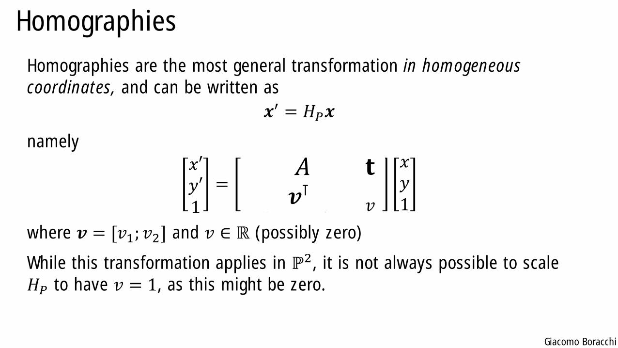
Homographies
Homographies are the most general transformation in homogeneous
coordinates, and can be written as
𝒙′ = 𝐻𝑃𝒙
namely
𝑥′𝑦′1
=𝜖 cos 𝜃𝜖 sin 𝜃0
− sin 𝜃cos 𝜃0
𝑡𝑥
𝑣
𝑥𝑦1
where 𝒗 = [𝑣1; 𝑣2] and 𝑣 ∈ ℝ (possibly zero)
While this transformation applies in ℙ2, it is not always possible to scale
𝐻𝑃 to have 𝑣 = 1, as this might be zero.
𝐴 𝐭𝒗⊺
Giacomo Boracchi
Homographies: Invariants
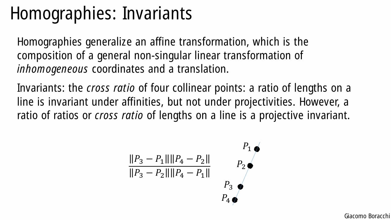
Homographies generalize an affine transformation, which is the
composition of a general non-singular linear transformation of
inhomogeneous coordinates and a translation.
Invariants: the cross ratio of four collinear points: a ratio of lengths on a
line is invariant under affinities, but not under projectivities. However, a
ratio of ratios or cross ratio of lengths on a line is a projective invariant.
𝑃3 − 𝑃1 𝑃4 − 𝑃2𝑃3 − 𝑃2 𝑃4 − 𝑃1
𝑃1
𝑃2
𝑃3𝑃4
Giacomo Boracchi
Homographies: Invariants
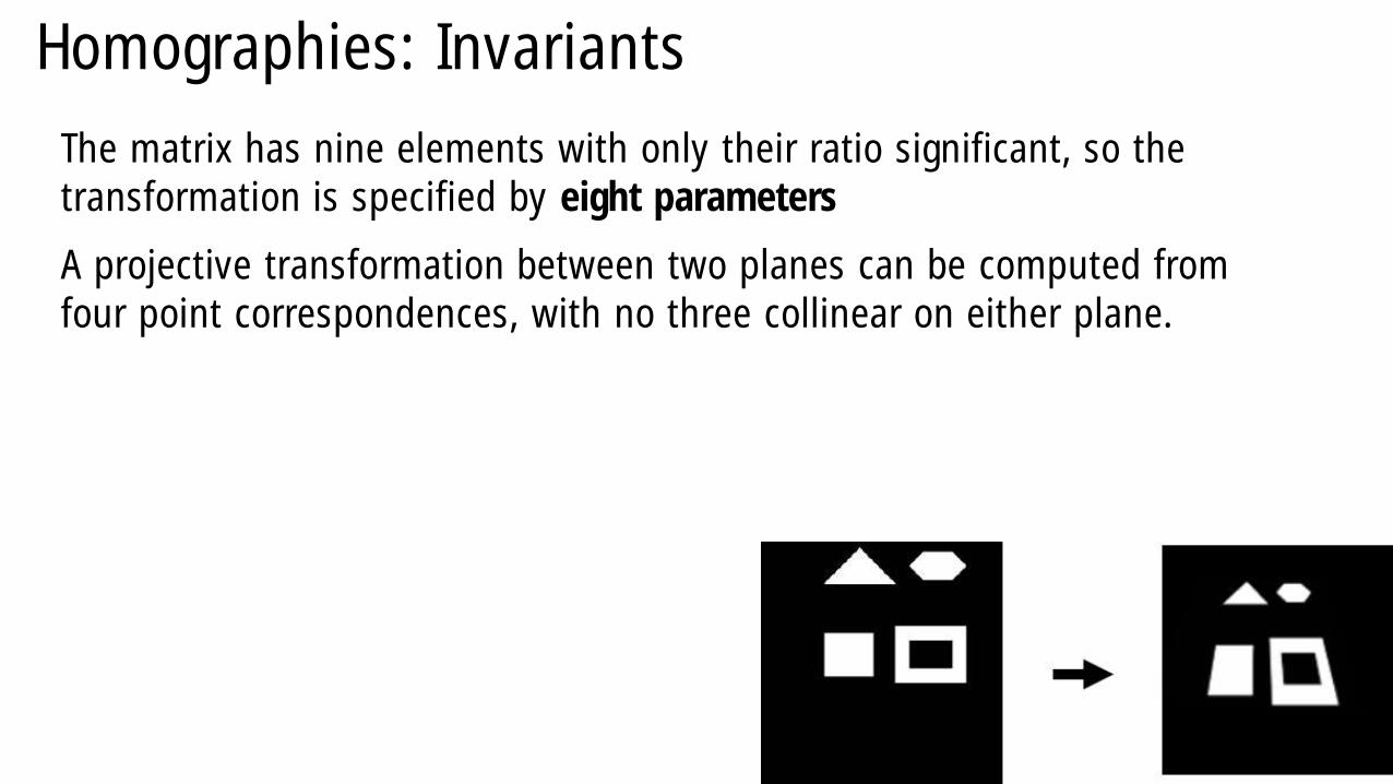
The matrix has nine elements with only their ratio significant, so the
transformation is specified by eight parameters
A projective transformation between two planes can be computed from
four point correspondences, with no three collinear on either plane.
Giacomo Boracchi
Homographies: Properties
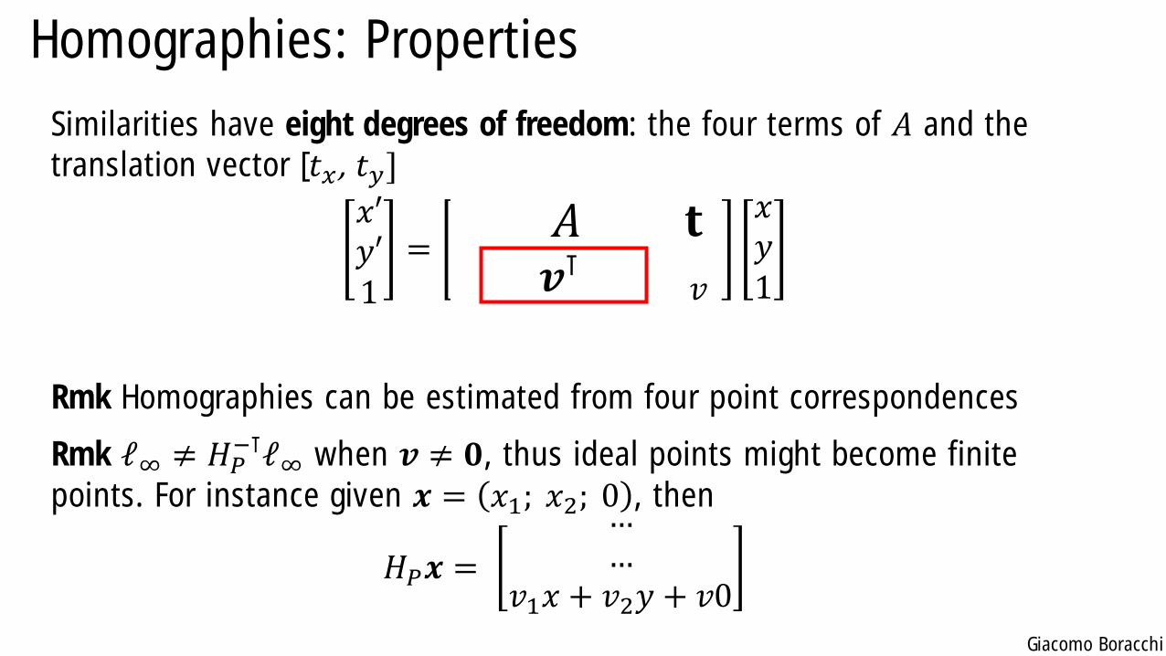
Similarities have eight degrees of freedom: the four terms of 𝐴 and the
translation vector [𝑡𝑥 , 𝑡𝑦]
𝑥′𝑦′1
=𝜖 cos 𝜃𝜖 sin 𝜃0
− sin 𝜃cos 𝜃0
𝑡𝑥
𝑣
𝑥𝑦1
Rmk Homographies can be estimated from four point correspondences
Rmk ℓ∞ ≠ 𝐻𝑃−⊺ℓ∞ when 𝒗 ≠ 𝟎, thus ideal points might become finite
points. For instance given 𝒙 = 𝑥1; 𝑥2; 0 , then
𝐻𝑃𝒙 =
……
𝑣1𝑥 + 𝑣2𝑦 + 𝑣0
𝐴 𝐭𝒗⊺
Giacomo Boracchi
Homographies: Properties
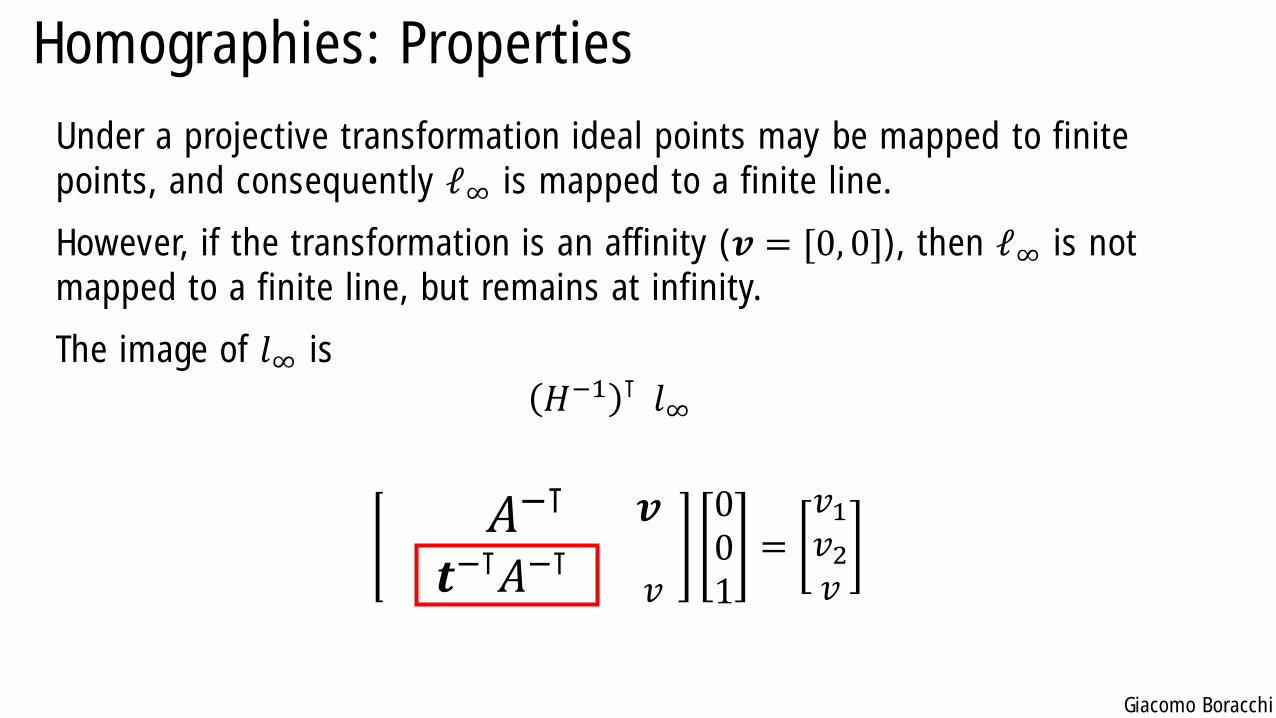
Under a projective transformation ideal points may be mapped to finite
points, and consequently ℓ∞ is mapped to a finite line.
However, if the transformation is an affinity (𝒗 = [0, 0]), then ℓ∞ is not
mapped to a finite line, but remains at infinity.
The image of 𝑙∞ is
𝐻−1 ⊺ 𝑙∞
𝜖 cos 𝜃𝜖 sin 𝜃0
− sin𝜃cos 𝜃0
𝑡𝑥
𝑣
001
=𝑣1𝑣2𝑣
𝐴−⊺ 𝒗
𝒕−⊺𝐴−⊺
Giacomo Boracchi
Affine Trasformation and Line at Infinity
Rmk: 𝑙∞ is not fixed pointwise under an affine transformation
Under an affinity a point on 𝑙∞ (i.e., an ideal point) can be mapped to a
different point on 𝑙∞. This is the reason why orthogonality is lost.
Giacomo Boracchi
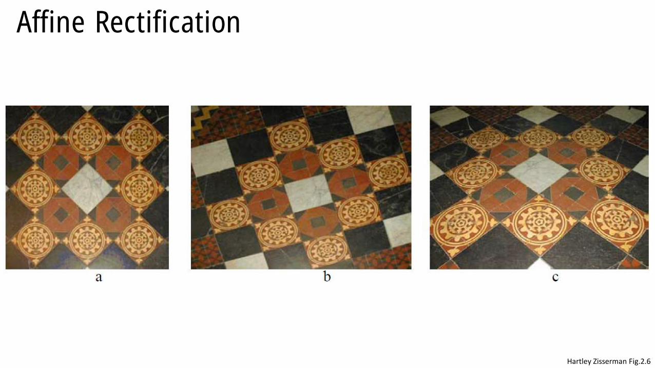
Affine Rectification
Hartley Zisserman Fig.2.6
Giacomo Boracchi
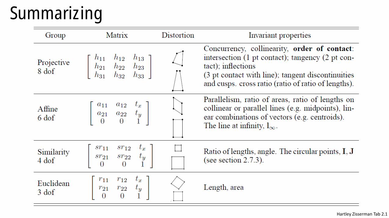
Summarizing
Hartley Zisserman Tab 2.1
Giacomo Boracchi
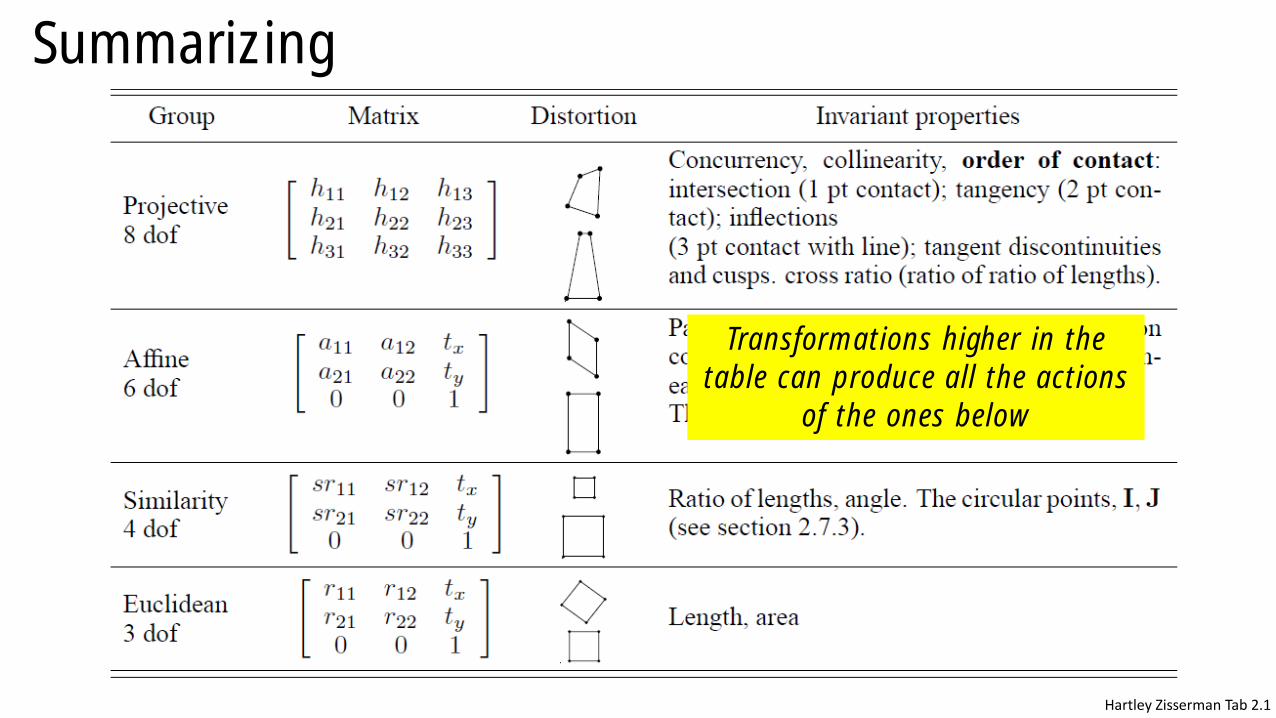
Summarizing
Hartley Zisserman Tab 2.1
Transformations higher in the
table can produce all the actions
of the ones below
Giacomo Boracchi
Homographies: Properties
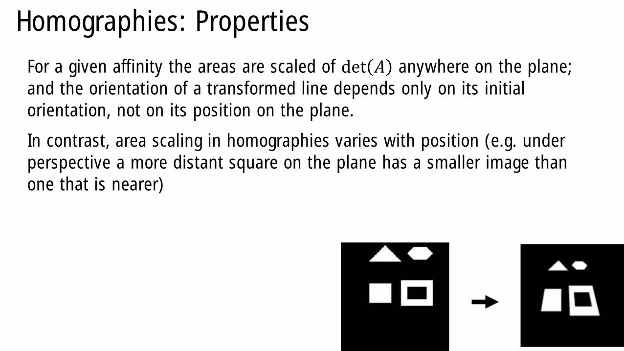
For a given affinity the areas are scaled of det 𝐴 anywhere on the plane;
and the orientation of a transformed line depends only on its initial
orientation, not on its position on the plane.
In contrast, area scaling in homographies varies with position (e.g. under
perspective a more distant square on the plane has a smaller image than
one that is nearer)

Giacomo Boracchi
The Projective Space ℙ3
Giacomo Boracchi
Points and Planes in ℙ3
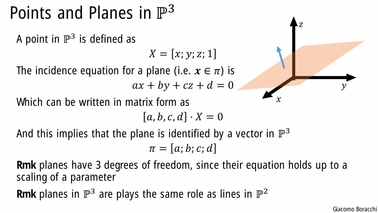
A point in ℙ3 is defined as
𝑋 = 𝑥; 𝑦; 𝑧; 1
The incidence equation for a plane (i.e. 𝒙 ∈ 𝜋) is
𝑎𝑥 + 𝑏𝑦 + 𝑐𝑧 + 𝑑 = 0
Which can be written in matrix form as
𝑎, 𝑏, 𝑐, 𝑑 ⋅ 𝑋 = 0
And this implies that the plane is identified by a vector in ℙ3
𝜋 = 𝑎; 𝑏; 𝑐; 𝑑
Rmk planes have 3 degrees of freedom, since their equation holds up to a scaling of a parameter
Rmk planes in ℙ3 are plays the same role as lines in ℙ2
𝑥
𝑦
𝑧
Giacomo Boracchi
Lines in ℙ3
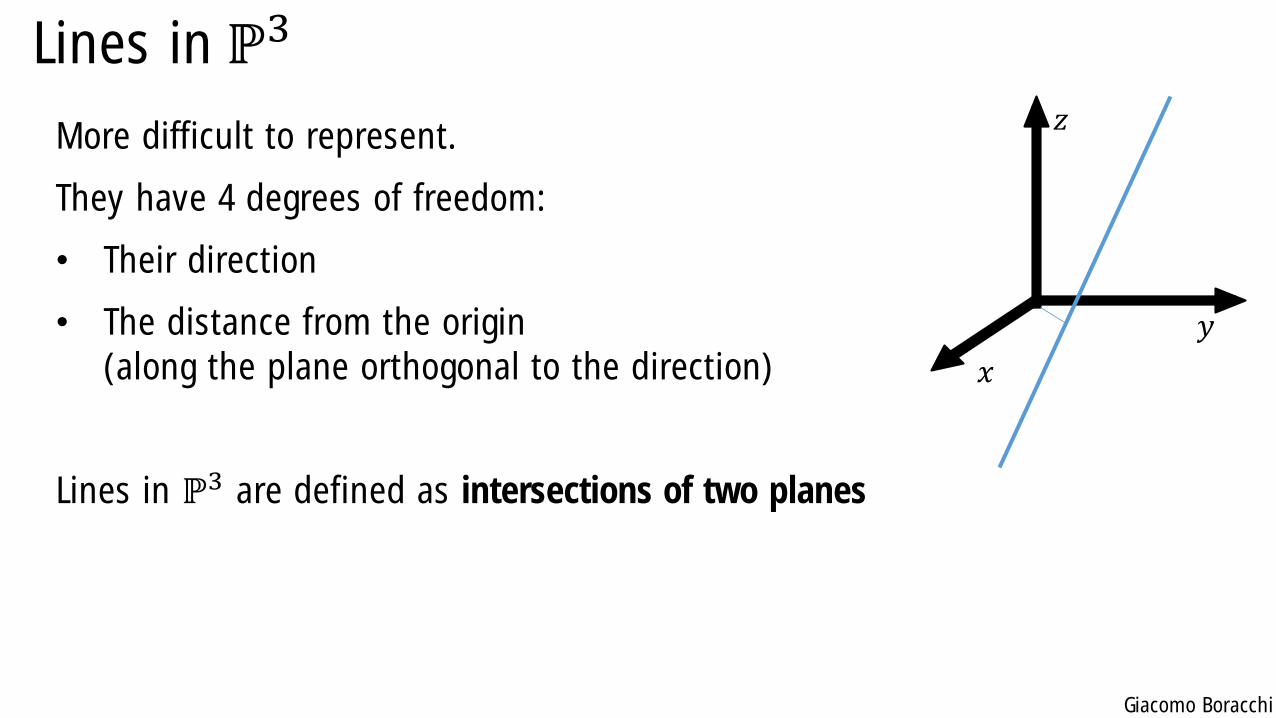
More difficult to represent.
They have 4 degrees of freedom:
• Their direction
• The distance from the origin
(along the plane orthogonal to the direction)
Lines in ℙ3 are defined as intersections of two planes
𝑥
𝑦
𝑧
Giacomo Boracchi
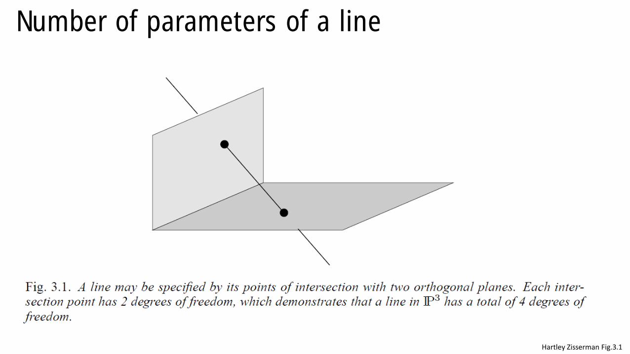
Number of parameters of a line
Hartley Zisserman Fig.3.1
Giacomo Boracchi
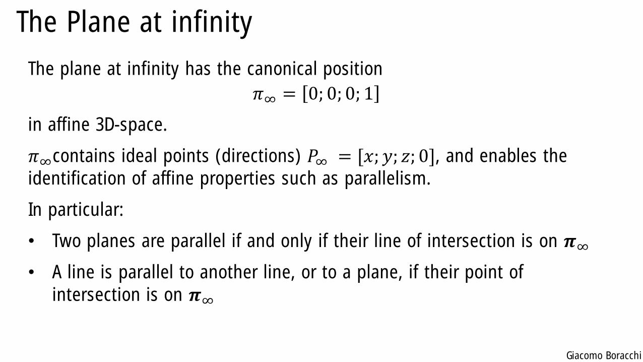
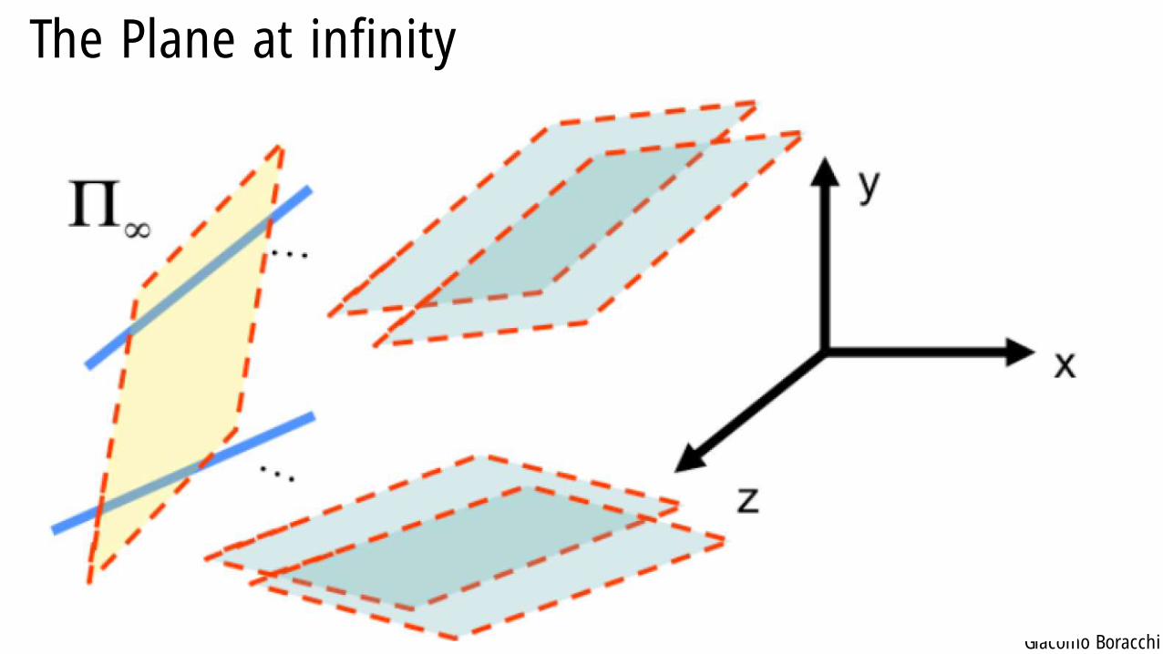
The Plane at infinity
The plane at infinity has the canonical position
𝜋∞ = 0; 0; 0; 1
in affine 3D-space.
𝜋∞contains ideal points (directions) 𝑃∞ = [𝑥; 𝑦; 𝑧; 0], and enables the
identification of affine properties such as parallelism.
In particular:
• Two planes are parallel if and only if their line of intersection is on 𝝅∞
• A line is parallel to another line, or to a plane, if their point of
intersection is on 𝝅∞
Giacomo Boracchi
The Plane at infinity
Giacomo Boracchi
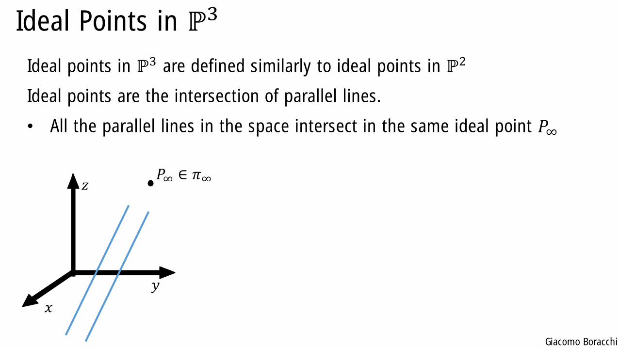
Ideal Points in ℙ3
Ideal points in ℙ3 are defined similarly to ideal points in ℙ2
Ideal points are the intersection of parallel lines.
• All the parallel lines in the space intersect in the same ideal point 𝑃∞
𝑥
𝑦
𝑧𝑃∞ ∈ 𝜋∞
Giacomo Boracchi
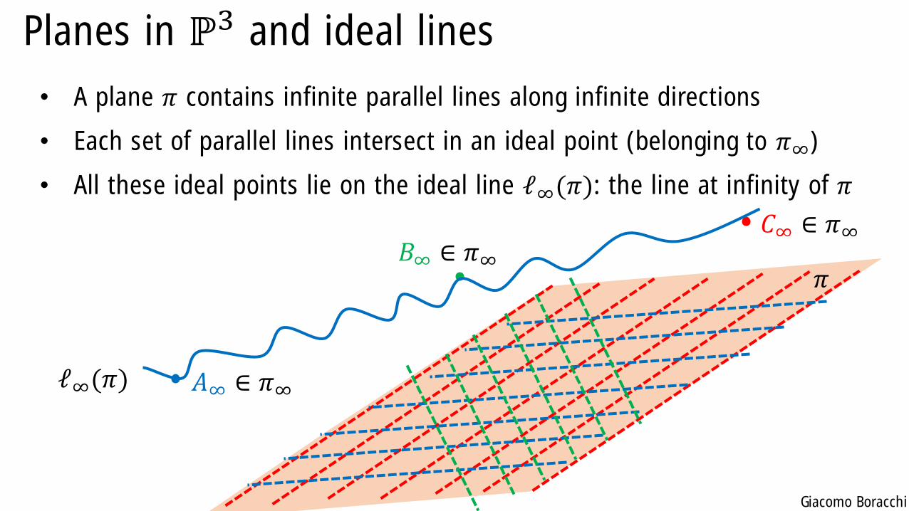
Planes in ℙ3 and ideal lines
• A plane 𝜋 contains infinite parallel lines along infinite directions
• Each set of parallel lines intersect in an ideal point (belonging to 𝜋∞)
• All these ideal points lie on the ideal line ℓ∞(𝜋): the line at infinity of 𝜋
𝐴∞ ∈ 𝜋∞
𝐶∞ ∈ 𝜋∞
𝜋
ℓ∞(𝜋)
𝐵∞ ∈ 𝜋∞
Giacomo Boracchi
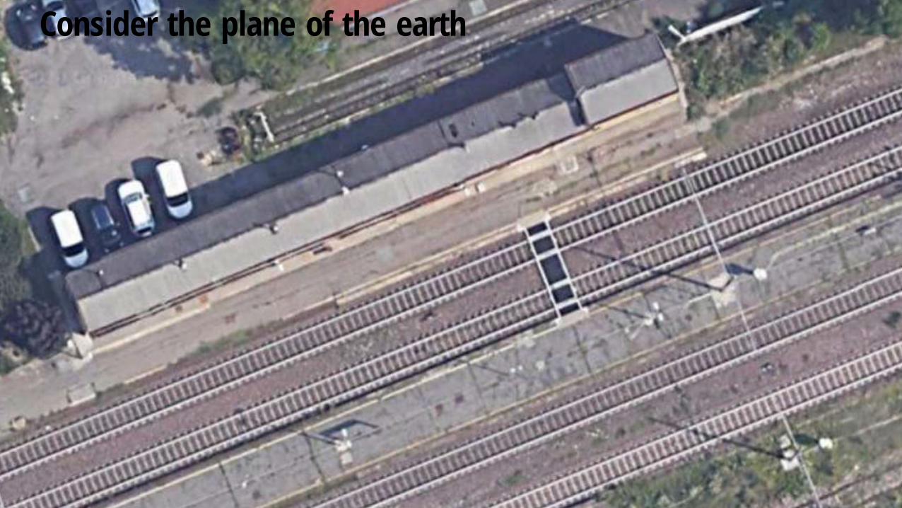
Consider the plane of the earth
Giacomo Boracchi
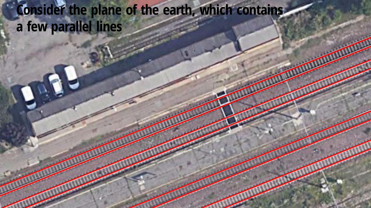
Consider the plane of the earth, which contains
a few parallel lines
Giacomo Boracchi
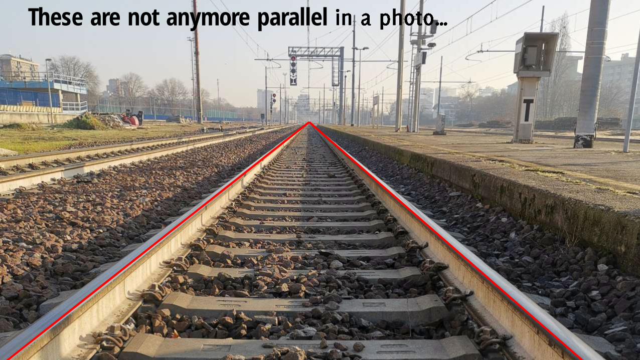
These are not anymore parallel
Giacomo Boracchi
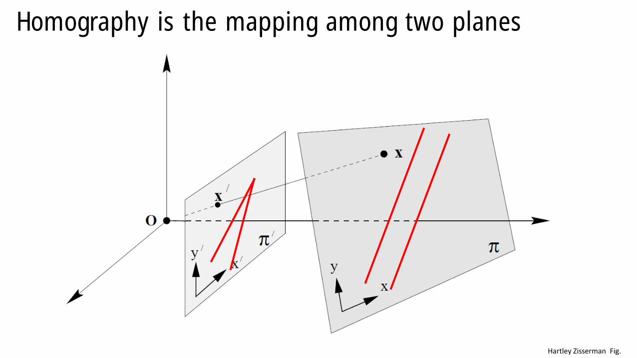
Homography is the mapping among two planes
Hartley Zisserman Fig.
Giacomo Boracchi
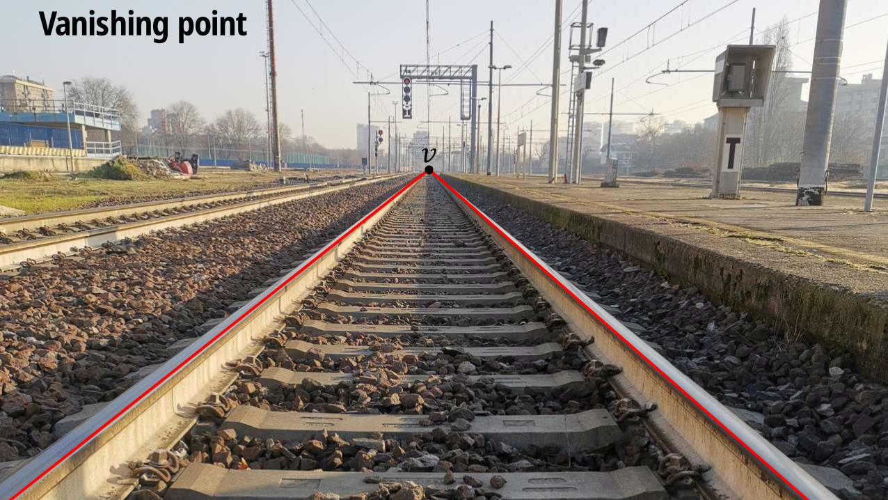
Vanishing point
𝑣
Giacomo Boracchi
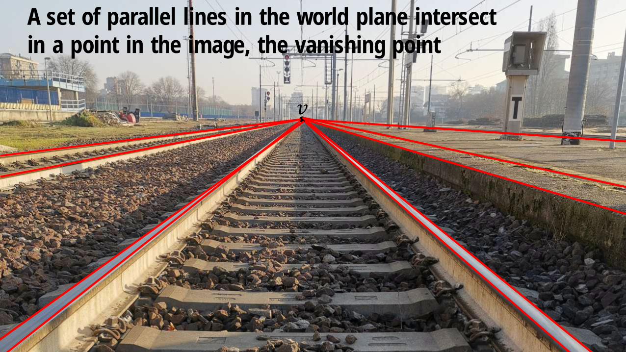
A set of parallel lines in the world plane intersect
in a point in the image, the vanishing point
𝑣
Giacomo Boracchi
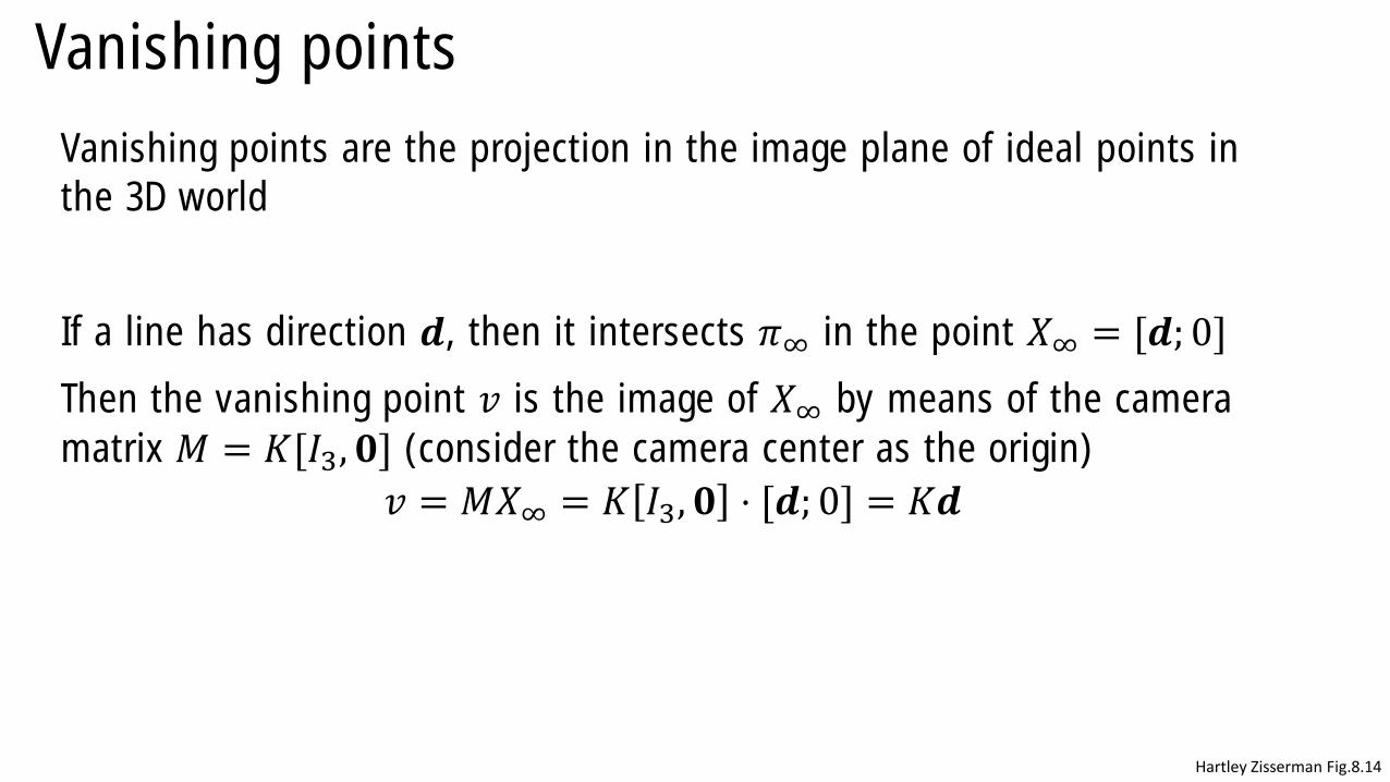
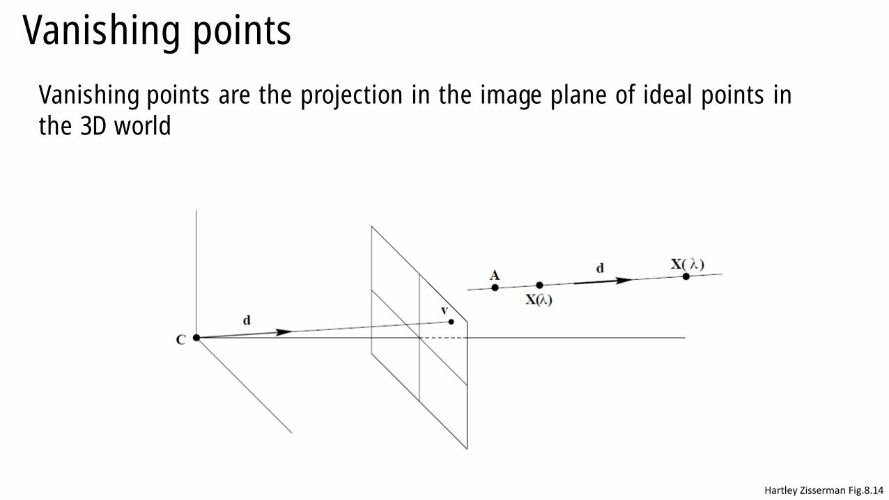
Vanishing points
Vanishing points are the projection in the image plane of ideal points in
the 3D world
If a line has direction 𝒅, then it intersects 𝜋∞ in the point 𝑋∞ = [𝒅; 0]
Then the vanishing point 𝑣 is the image of 𝑋∞ by means of the camera
matrix 𝑀 = 𝐾[𝐼3, 𝟎] (consider the camera center as the origin)
𝑣 = 𝑀𝑋∞ = 𝐾 𝐼3, 𝟎 ⋅ [𝒅; 0] = 𝐾𝒅
Hartley Zisserman Fig.8.14
Giacomo Boracchi
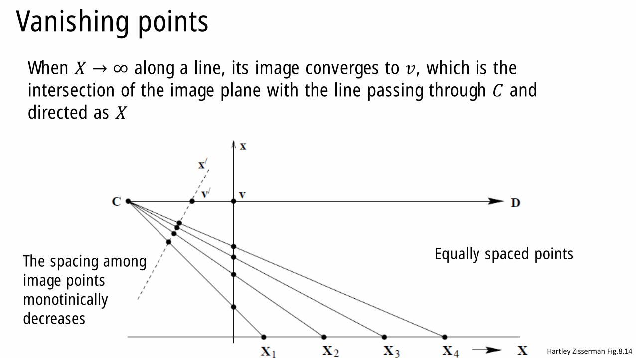
Vanishing points
When 𝑋 → ∞ along a line, its image converges to 𝑣, which is the
intersection of the image plane with the line passing through 𝐶 and
directed as 𝑋
Hartley Zisserman Fig.8.14
Equally spaced pointsThe spacing among
image points
monotinically
decreases
Giacomo Boracchi
Vanishing points
Vanishing points are the projection in the image plane of ideal points in
the 3D world
Hartley Zisserman Fig.8.14
Giacomo Boracchi
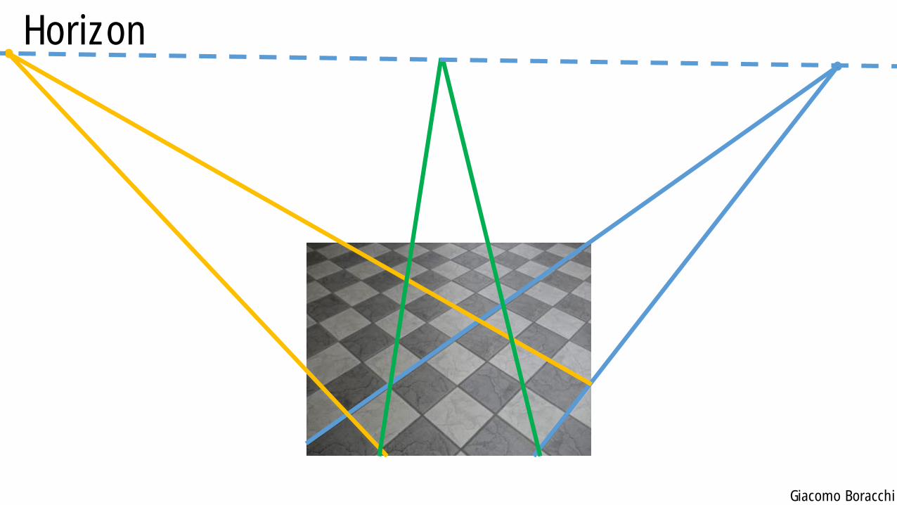
Horizon
Horizon or Vanishing line for a plane 𝜋 is the image of the line at the
infinity of that plane, ℓ∞(𝜋)
Horizon helps humans to intuitively deduce properties about the image
that might not be apparent mathematically.
We can understand when two lines are parallel in the 3D world, since they
intersect with the horizon
Giacomo Boracchi
Horizon
Giacomo Boracchi
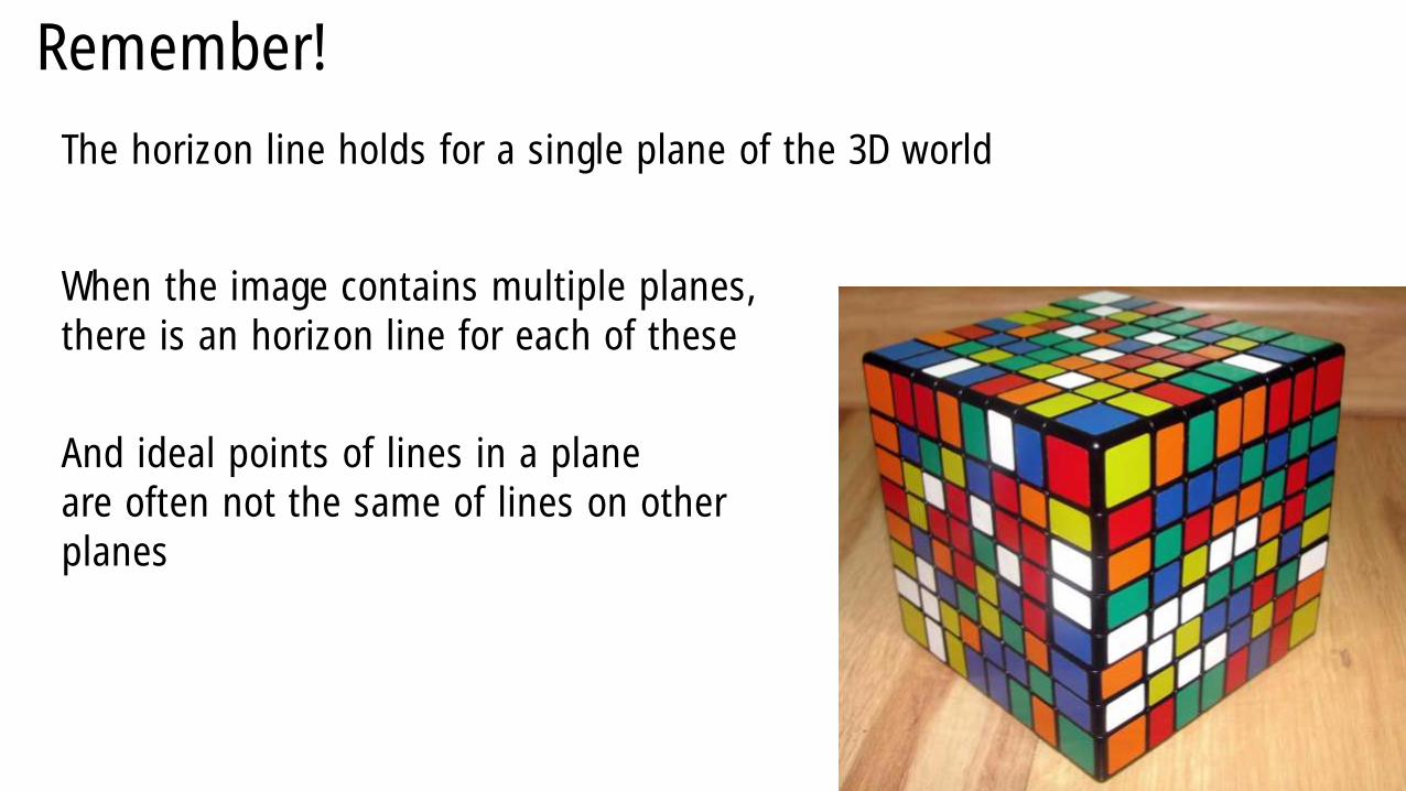
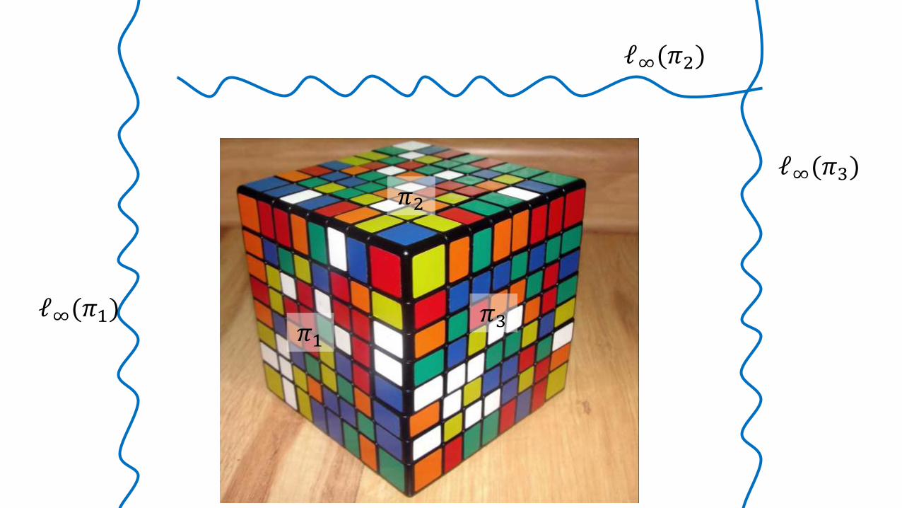
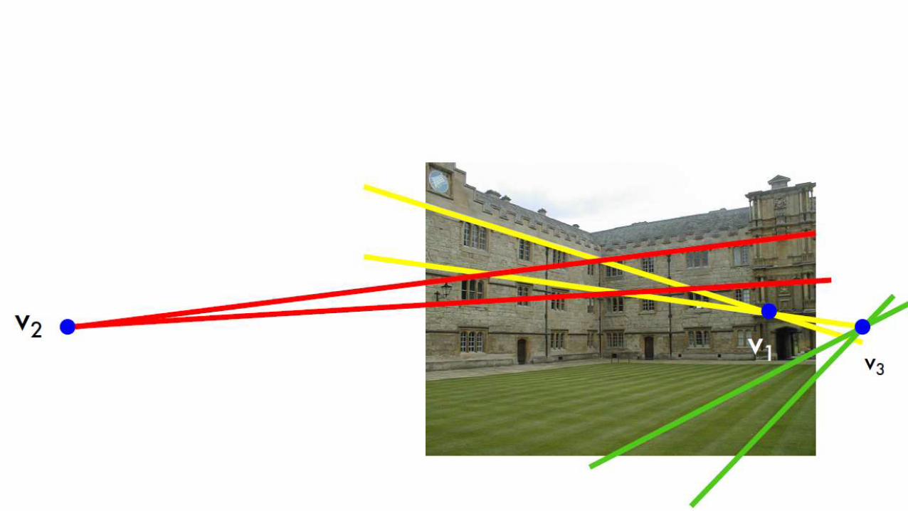
Remember!
The horizon line holds for a single plane of the 3D world
When the image contains multiple planes,
there is an horizon line for each of these
And ideal points of lines in a plane
are often not the same of lines on other
planes
Giacomo Boracchi
ℓ∞(𝜋3)
ℓ∞(𝜋1)
ℓ∞(𝜋2)
𝜋3𝜋1
𝜋2
Giacomo Boracchi
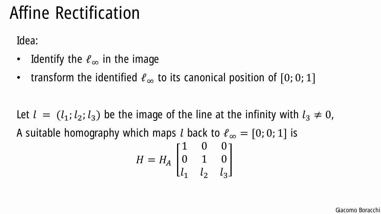
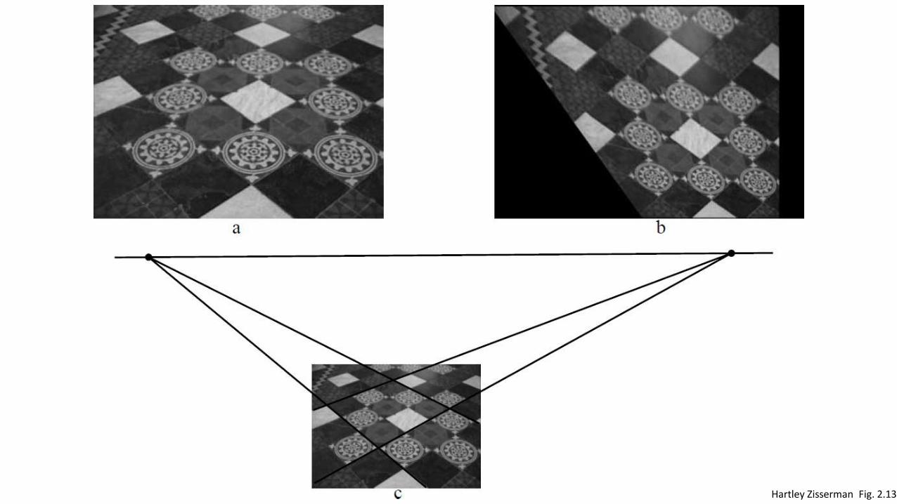
Affine Rectification
Idea:
• Identify the ℓ∞ in the image
• transform the identified ℓ∞ to its canonical position of [0; 0; 1]
Let 𝑙 = (𝑙1; 𝑙2; 𝑙3) be the image of the line at the infinity with 𝑙3 ≠ 0,
A suitable homography which maps 𝑙 back to ℓ∞ = [0; 0; 1] is
𝐻 = 𝐻𝐴
1 0 00 1 0𝑙1 𝑙2 𝑙3
Giacomo Boracchi
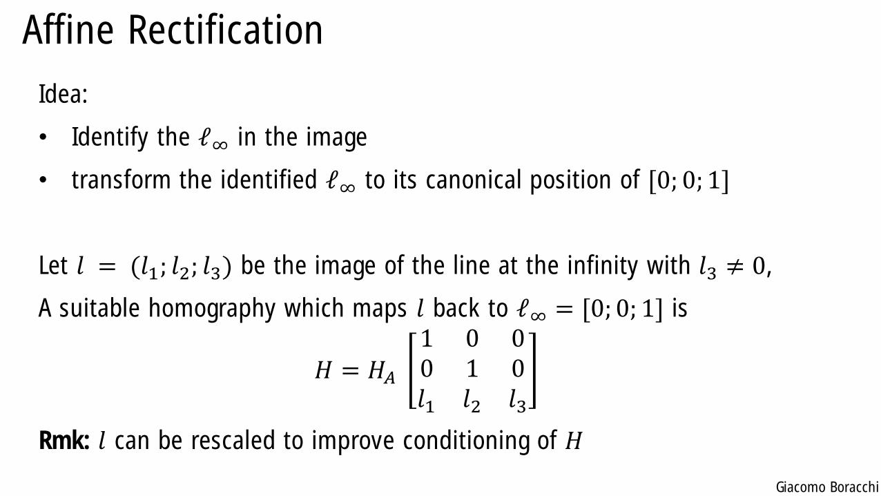
Affine Rectification
Idea:
• Identify the ℓ∞ in the image
• transform the identified ℓ∞ to its canonical position of [0; 0; 1]
Let 𝑙 = (𝑙1; 𝑙2; 𝑙3) be the image of the line at the infinity with 𝑙3 ≠ 0,
A suitable homography which maps 𝑙 back to ℓ∞ = [0; 0; 1] is
𝐻 = 𝐻𝐴
1 0 00 1 0𝑙1 𝑙2 𝑙3
Rmk: 𝑙 can be rescaled to improve conditioning of 𝐻
Giacomo Boracchi
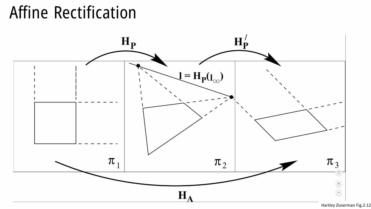
Affine Rectification
Hartley Zisserman Fig.2.12
Giacomo BoracchiHartley Zisserman Fig. 2.13
Giacomo Boracchi
Single-View GeometryGiacomo Boracchi
March 3rd, 2020
USI, Lugano
Book: HZ, chapter 2,3
Giacomo Boracchi
Outline
• DLT Algorithm for Least Squares Fitting in ℙ2
• Homography estimation
• Camera Calibration
• Applying Point Trasformations to Images
• Conics in ℙ2
• Conic Fitting
Giacomo Boracchi
DLT algorithm
HZ chapter 4
Giacomo Boracchi
DLT
Direct Linear Trasformation (DLT) algorithm, solves many relevant
problems in Computer Vision
• 2D Homography estimation
• Camera projection matrix estimation (projections from 3D to 2D)
• Fundamental matrix computation
• Trifocal tensor computation
Giacomo Boracchi
Homography estimation
We consider a set of point correspondences
𝒙𝒊′, 𝒙𝒊 , 𝑖 = 1,… , 4
belonging to two different images. Our problem is to compute a 𝐻 ∈ ℝ3×3
such that 𝒙𝒊′ = 𝐻𝒙𝒊 for each 𝑖.
Rmk if we look at 𝒙 as a 3d vector the equality 𝒙𝒊′ = 𝐻𝒙𝒊 does not hold
Equality holds in ℙ2 (but linear systems are solved as in ℝ3).
What makes the DLT is distinct from standard cases since the left and
right sides of the defining equation can differ by an unknown
multiplicative factor which is dependent on the number of equations.
Giacomo Boracchi
DLT for Homography Estimation
In ℝ3, 𝒙𝒊′ and 𝒙𝒊 have the same direction, but may differ in magnitude.
Therefore collinearity constraints can be written as
𝒙𝒊′ × 𝐻𝒙𝒊 = 𝟎 , 𝑖 = 1,… , 4
where 𝟎 = [0; 0; 0]
By Acdx - Self-made
Giacomo Boracchi
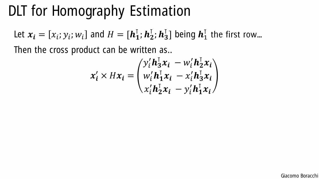
DLT for Homography Estimation
Let 𝒙𝒊 = 𝑥𝑖; 𝑦𝑖; 𝑤𝑖 and 𝐻 = [𝒉𝟏⊺ ; 𝒉𝟐
⊺ ; 𝒉𝟑⊺ ] being 𝒉1
⊺
Then the cross product can be written as..
𝒙𝒊′ × 𝐻𝒙𝒊 =
𝑦𝑖′𝒉𝟑
⊺ 𝒙𝒊 −𝑤𝑖′𝒉𝟐
⊺ 𝒙𝒊𝑤𝑖′𝒉𝟏
⊺ 𝒙𝒊 − 𝑥𝑖′𝒉𝟑
⊺ 𝒙𝒊𝑥𝑖′𝒉𝟐
⊺ 𝒙𝒊 − 𝑦𝑖′𝒉𝟏
⊺ 𝒙𝒊
Giacomo Boracchi
DLT for Homography Estimation
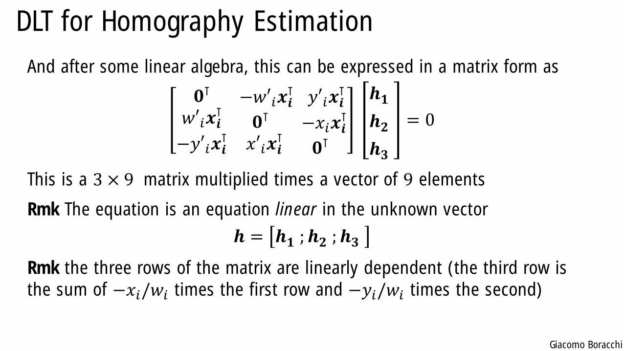
And after some linear algebra, this can be expressed in a matrix form as
𝟎⊺
𝑤′𝑖𝒙𝒊⊺
−𝑦′𝑖𝒙𝒊⊺
−𝑤′𝑖𝒙𝒊⊺
𝟎⊺
𝑥′𝑖𝒙𝒊⊺
𝑦′𝑖𝒙𝒊⊺
−𝑥𝑖𝒙𝒊⊺
𝟎⊺
𝒉𝟏
𝒉𝟐
𝒉𝟑
= 0
This is a 3 × 9 matrix multiplied times a vector of 9 elements
Rmk The equation is an equation linear in the unknown vector
𝒉 = 𝒉𝟏 ; 𝒉𝟐 ; 𝒉𝟑
Rmk the three rows of the matrix are linearly dependent (the third row is
the sum of −𝑥𝑖/𝑤𝑖 times the first row and −𝑦𝑖/𝑤𝑖 times the second)
Giacomo Boracchi
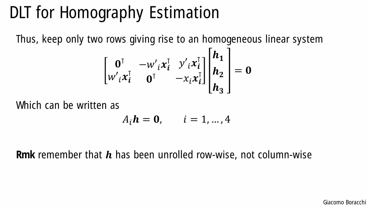
DLT for Homography Estimation
Thus, keep only two rows giving rise to an homogeneous linear system
𝟎⊺
𝑤′𝑖𝒙𝒊⊺−𝑤′𝑖𝒙𝒊
⊺
𝟎⊺𝑦′𝑖𝒙𝒊
⊺
−𝑥𝑖𝒙𝒊⊺
𝒉𝟏
𝒉𝟐
𝒉𝟑
= 𝟎
Which can be written as
𝐴𝑖𝒉 = 𝟎, 𝑖 = 1,… , 4
Rmk remember that 𝒉 has been unrolled row-wise, not column-wise
Giacomo Boracchi
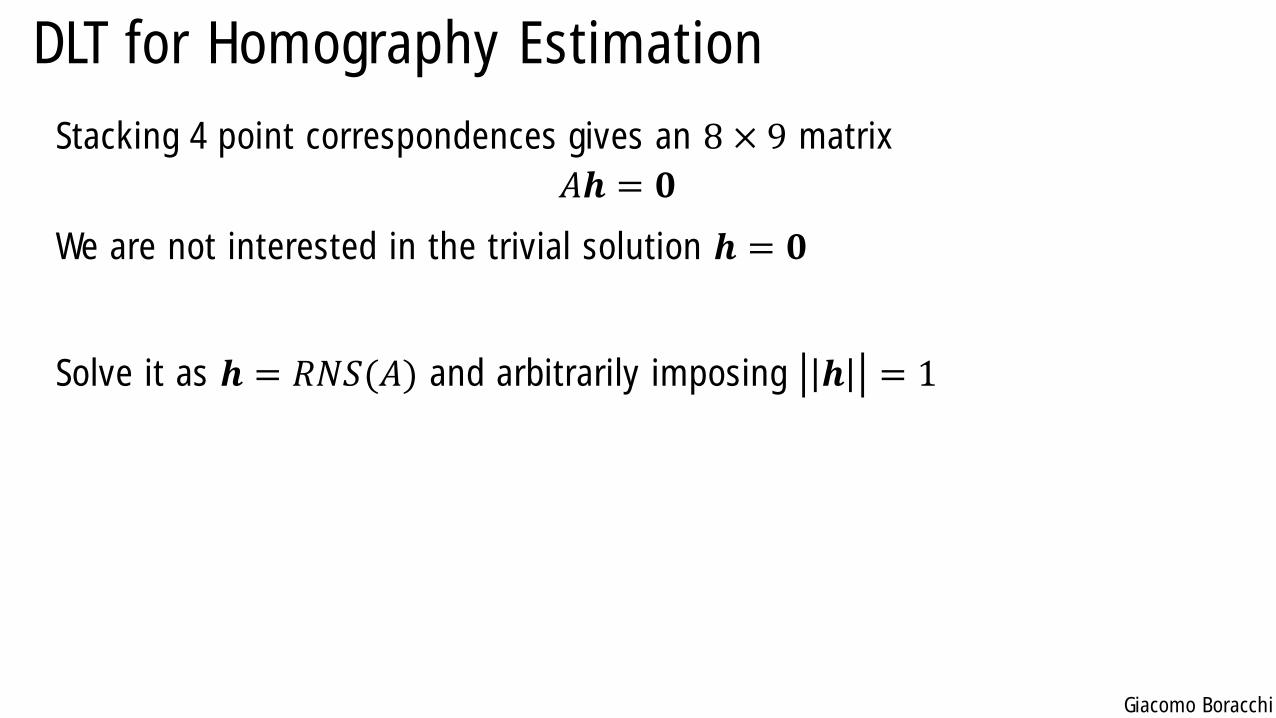
DLT for Homography Estimation
Stacking 4 point correspondences gives an 8 × 9 matrix
𝐴𝒉 = 𝟎
We are not interested in the trivial solution 𝒉 = 𝟎
Solve it as 𝒉 = 𝑅𝑁𝑆(𝐴) and arbitrarily imposing 𝒉 = 1
Giacomo Boracchi
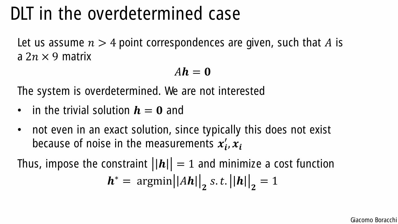
DLT in the overdetermined case
Let us assume 𝑛 > 4 point correspondences are given, such that 𝐴 is
a 2𝑛 × 9 matrix
𝐴𝒉 = 𝟎
The system is overdetermined. We are not interested
• in the trivial solution 𝒉 = 𝟎 and
• not even in an exact solution, since typically this does not exist
because of noise in the measurements 𝒙𝒊′, 𝒙𝒊
Thus, impose the constraint 𝒉 = 1 and minimize a cost function
𝒉∗ = argmin 𝐴𝒉𝟐𝑠. 𝑡. 𝒉
𝟐= 1
Giacomo Boracchi
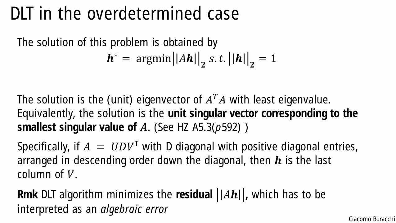
DLT in the overdetermined case
The solution of this problem is obtained by
𝒉∗ = argmin 𝐴𝒉𝟐𝑠. 𝑡. 𝒉
𝟐= 1
The solution is the (unit) eigenvector of 𝐴𝑇𝐴 with least eigenvalue.
Equivalently, the solution is the unit singular vector corresponding to the
smallest singular value of 𝑨. (See HZ A5.3(p592) )
Specifically, if 𝐴 = 𝑈𝐷𝑉⊺ with D diagonal with positive diagonal entries,
arranged in descending order down the diagonal, then 𝒉 is the last
column of 𝑉.
Rmk DLT algorithm minimizes the residual 𝐴𝒉 , which has to be
interpreted as an algebraic error
Giacomo Boracchi
DLT and the reference system
Are the outcome of DLT independent of the reference system being used
to express 𝒙′ and 𝒙?
Unfortunately DLT is not invariant to similarity transformations.
Therefore, it is necessary to apply a normalizing transformation to the
data before applying the DLT algorithm.
Normalizing the data makes the DLT invariant to the reference system, as
it is always being estimated in a canonical reference
Normalization is also called Pre-conditioning
Giacomo Boracchi
Preconditioning
Needed because in homogeneous coordinate systems, components
typically have very different ranges
• Row and Column indexes ranges in [0 − 4𝐾]
• Third component is 1
Define a maping
𝑥 → 𝑇𝑥
That brings all the points «aronud the origin» and rescale each component
to the same range (say at an average distance 2 from the origin)
Giacomo Boracchi
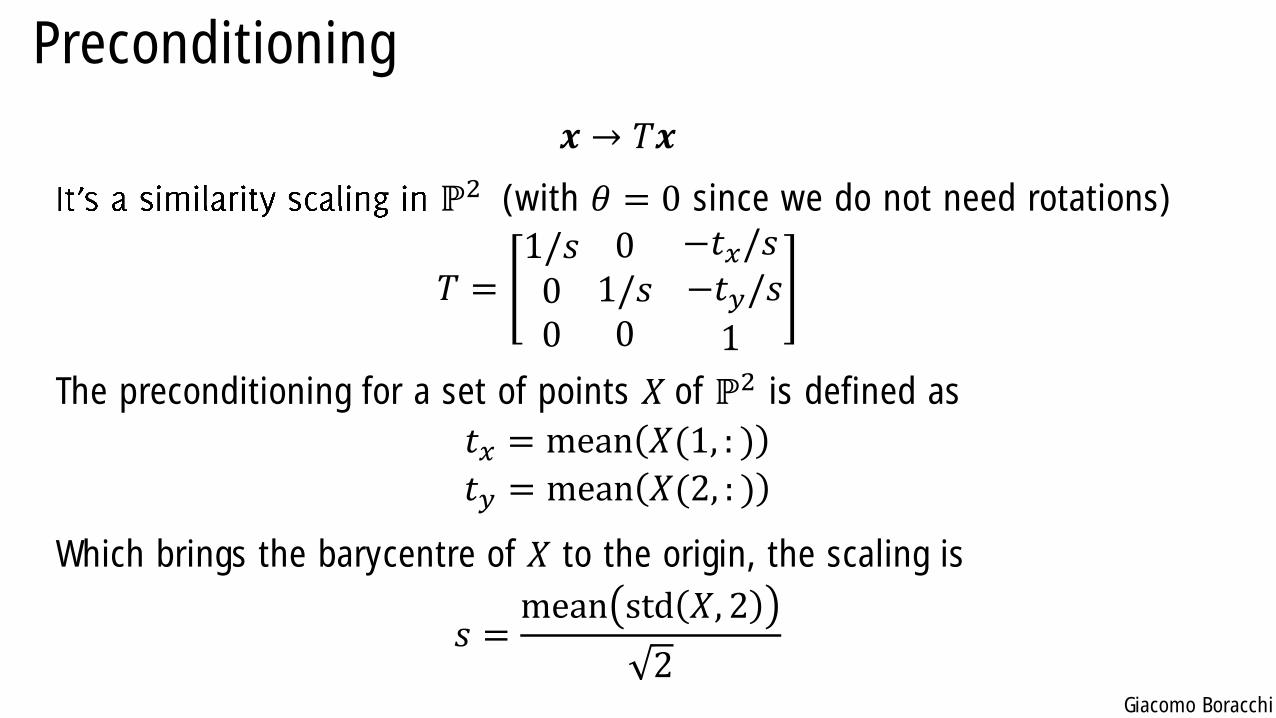
Preconditioning
𝒙 → 𝑇𝒙
ℙ2 (with 𝜃 = 0 since we do not need rotations)
𝑇 =1/𝑠00
01/𝑠0
−𝑡𝑥/𝑠−𝑡𝑦/𝑠
1
The preconditioning for a set of points 𝑋 of ℙ2 is defined as
𝑡𝑥 = mean 𝑋(1, : )
𝑡𝑦 = mean 𝑋(2, : )
Which brings the barycentre of 𝑋 to the origin, the scaling is
𝑠 =mean std 𝑋, 2
2
Giacomo Boracchi
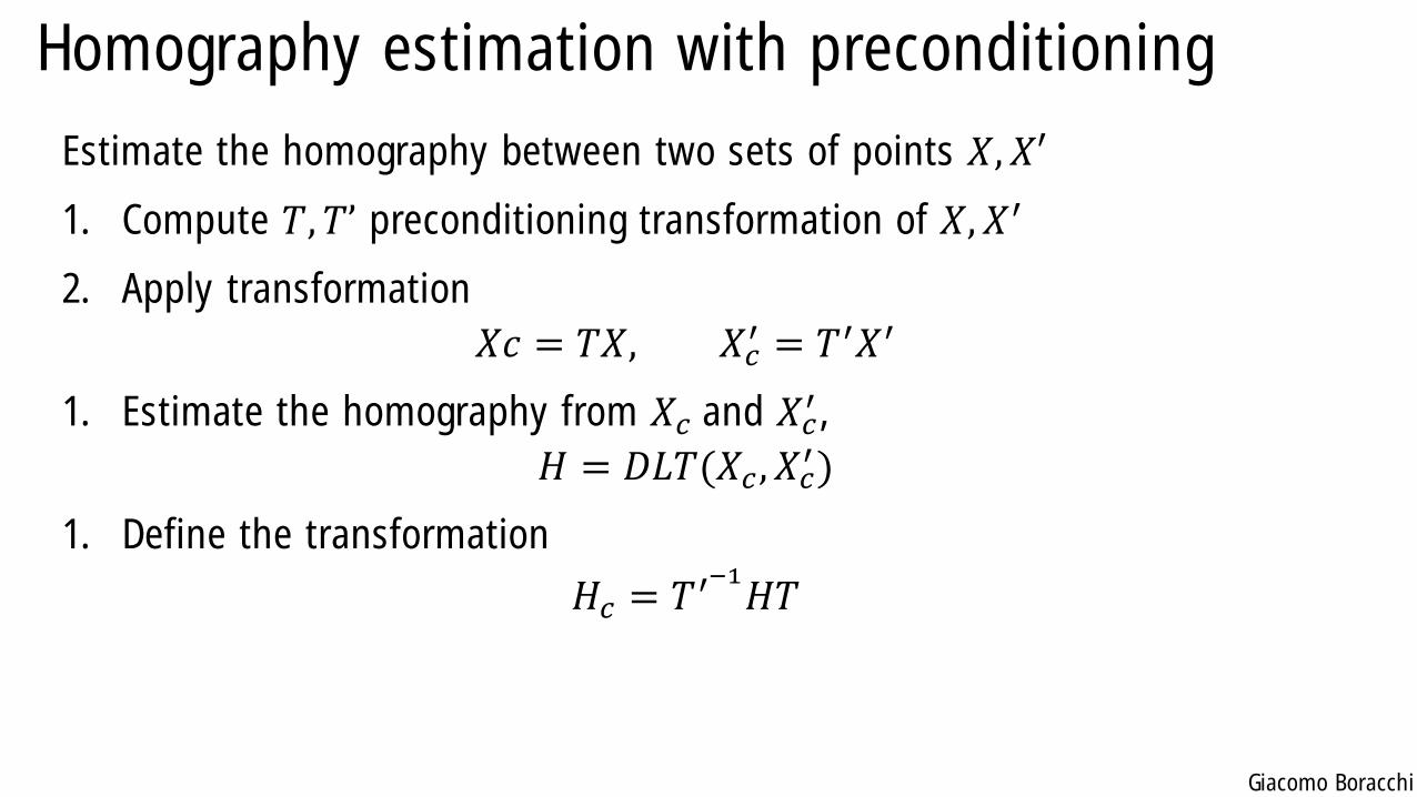
Homography estimation with preconditioning
Estimate the homography between two sets of points 𝑋, 𝑋′
1. Compute 𝑇, 𝑇’ preconditioning transformation of 𝑋, 𝑋′
2. Apply transformation
𝑋𝑐 = 𝑇𝑋, 𝑋𝑐′ = 𝑇′𝑋′
1. Estimate the homography from 𝑋𝑐 and 𝑋𝑐′ ,
𝐻 = 𝐷𝐿𝑇(𝑋𝑐 , 𝑋𝑐′)
1. Define the transformation
𝐻𝑐 = 𝑇′−1𝐻𝑇
Giacomo Boracchi
How to apply linear transformations to an image?
pixel intensities
Giacomo Boracchi
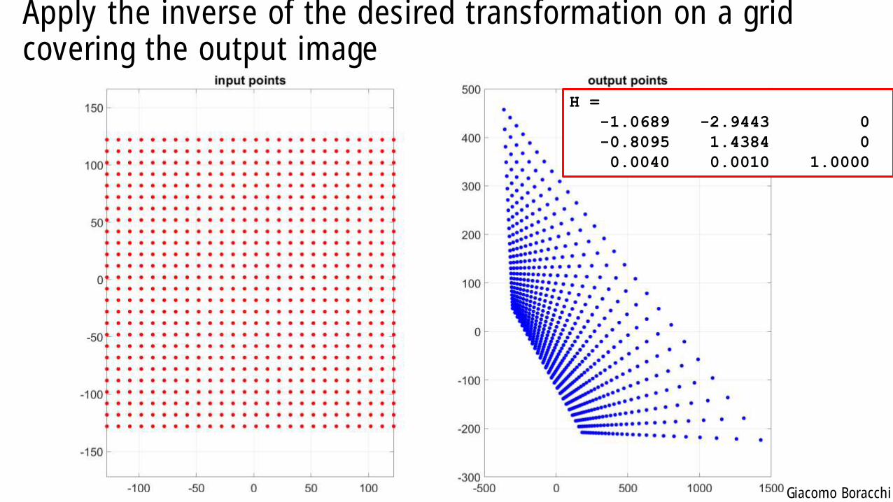
Apply the inverse of the desired transformation on a grid covering the output image
H =
-1.0689 -2.9443 0
-0.8095 1.4384 0
0.0040 0.0010 1.0000
Giacomo Boracchi
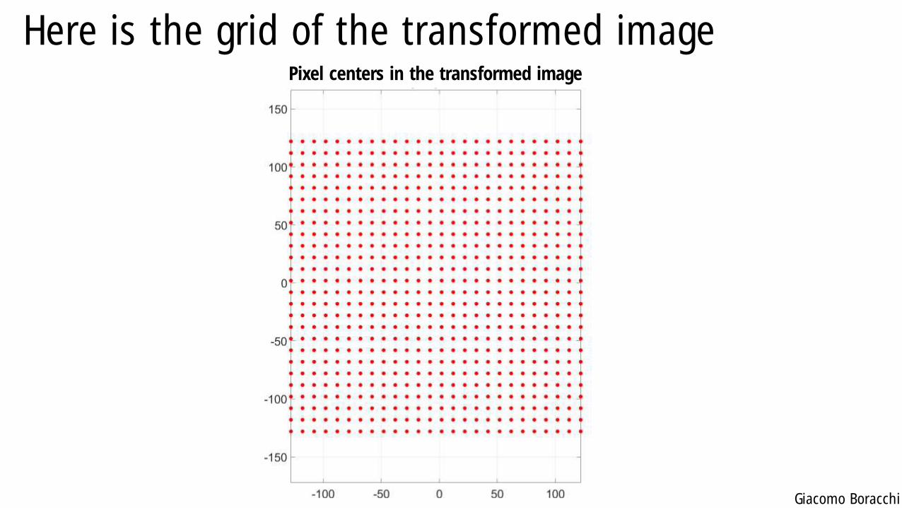
Here is the grid of the transformed imagePixel centers in the transformed image
Giacomo Boracchi
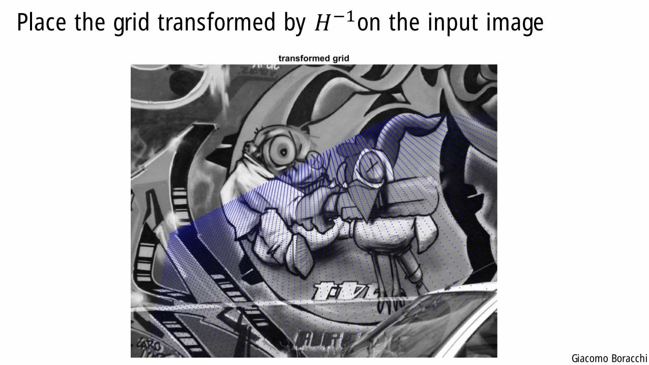
Place the grid transformed by 𝐻−1on the input image
Giacomo Boracchi
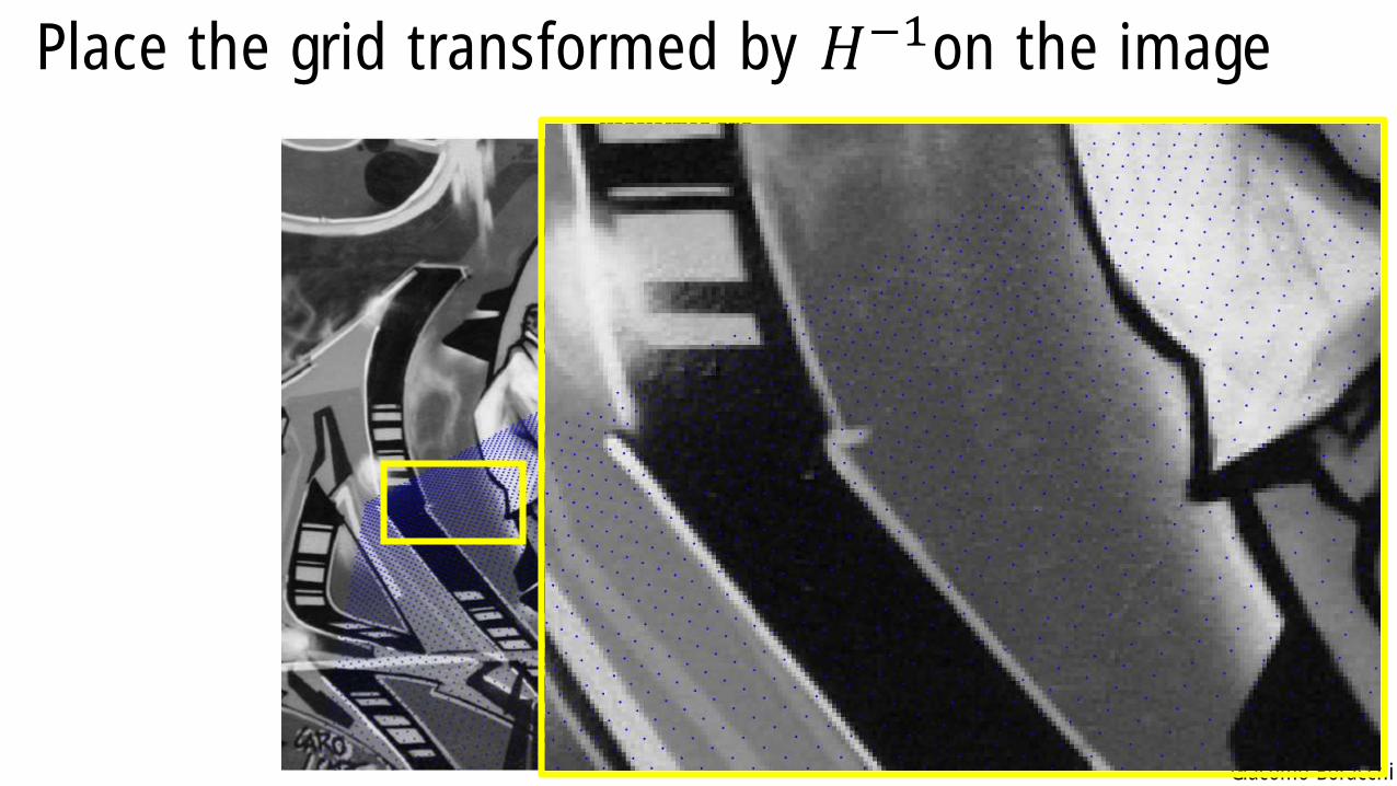
Place the grid transformed by 𝐻−1on the image
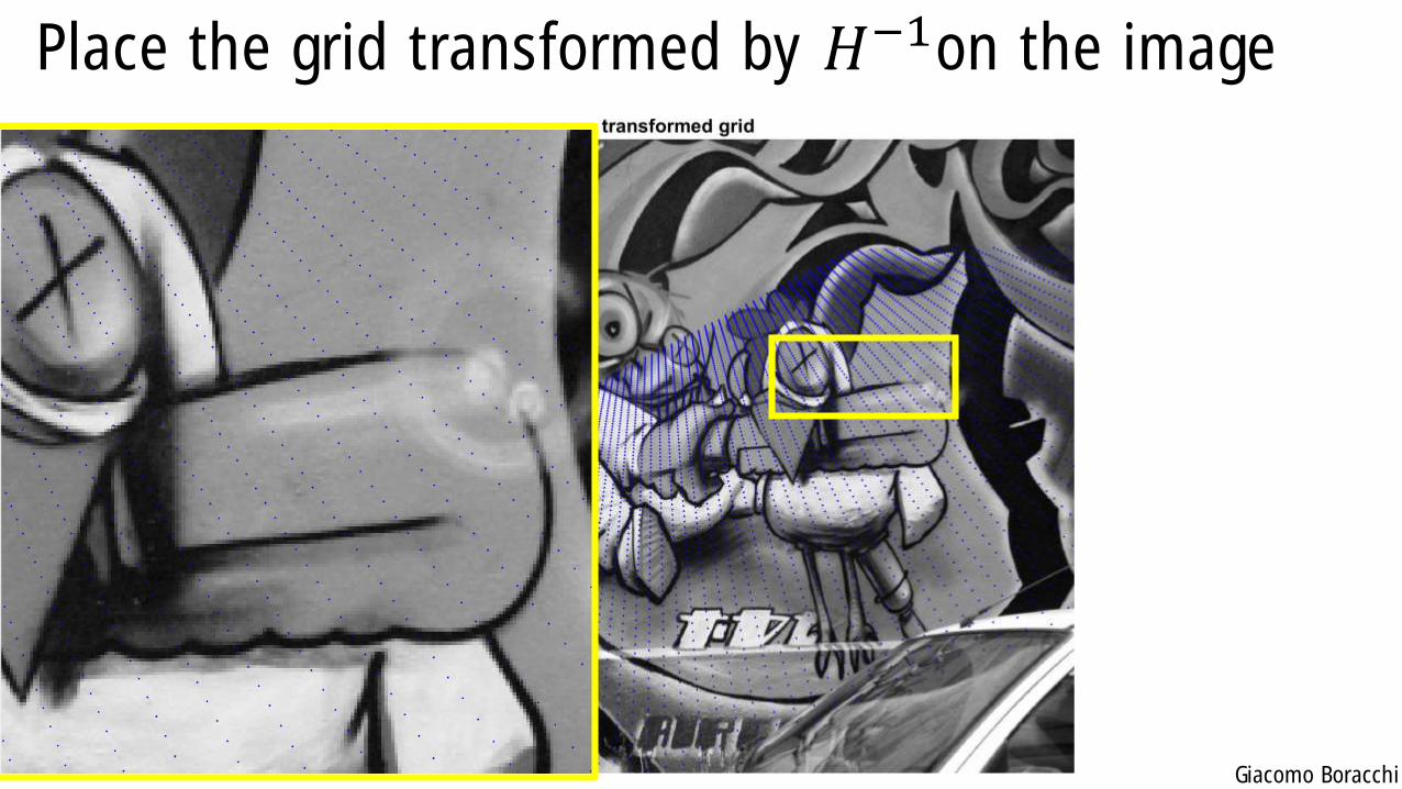
Giacomo Boracchi
Place the grid transformed by 𝐻−1on the image
Giacomo Boracchi
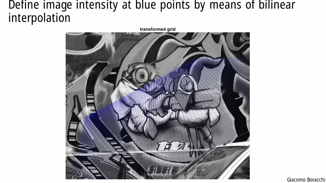
Define image intensity at blue points by means of bilinear interpolation
Giacomo Boracchi
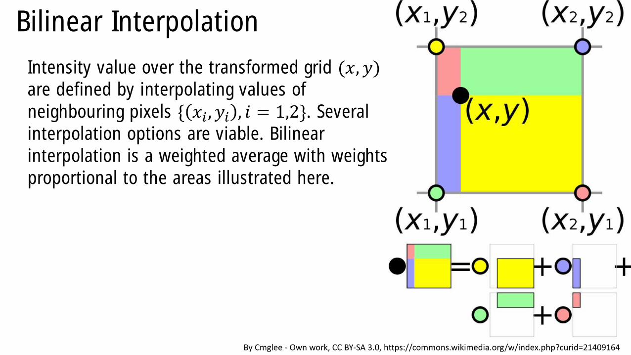
Bilinear Interpolation
Intensity value over the transformed grid (𝑥, 𝑦)are defined by interpolating values of
neighbouring pixels { 𝑥𝑖 , 𝑦𝑖 , 𝑖 = 1,2}. Several
interpolation options are viable. Bilinear
interpolation is a weighted average with weights
proportional to the areas illustrated here.
By Cmglee - Own work, CC BY-SA 3.0, https://commons.wikimedia.org/w/index.php?curid=21409164
Giacomo Boracchi
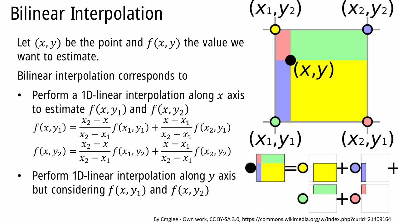
Bilinear Interpolation
Let (𝑥, 𝑦) be the point and 𝑓(𝑥, 𝑦) the value we
want to estimate.
Bilinear interpolation corresponds to
• Perform a 1D-linear interpolation along 𝑥 axis
to estimate 𝑓 𝑥, 𝑦1 and 𝑓 𝑥, 𝑦2
𝑓 𝑥, 𝑦1 =𝑥2 − 𝑥
𝑥2 − 𝑥1𝑓 𝑥1, 𝑦1 +
𝑥 − 𝑥1𝑥2 − 𝑥1
𝑓 𝑥2, 𝑦1
𝑓 𝑥, 𝑦2 =𝑥2 − 𝑥
𝑥2 − 𝑥1𝑓 𝑥1, 𝑦2 +
𝑥 − 𝑥1𝑥2 − 𝑥1
𝑓 𝑥2, 𝑦2
• Perform 1D-linear interpolation along 𝑦 axis
but considering 𝑓(𝑥, 𝑦1) and 𝑓(𝑥, 𝑦2)
By Cmglee - Own work, CC BY-SA 3.0, https://commons.wikimedia.org/w/index.php?curid=21409164
Giacomo Boracchi
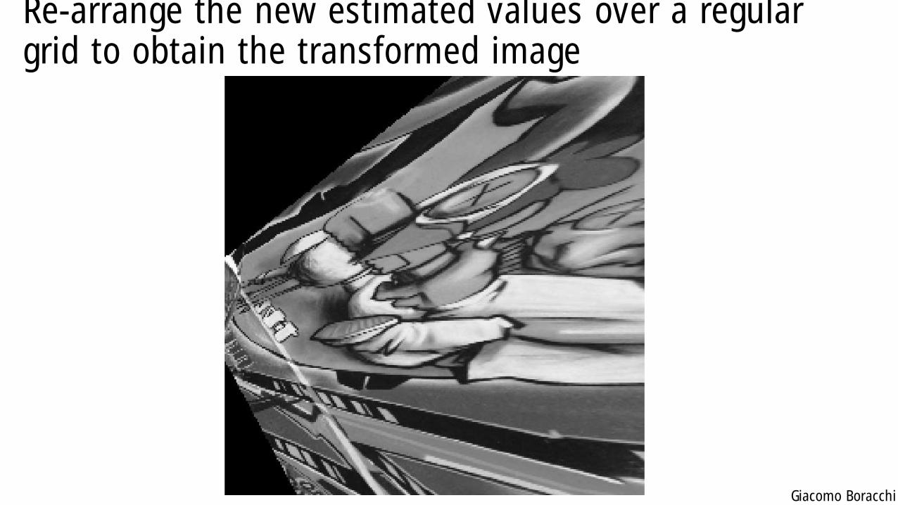
Re-arrange the new estimated values over a regular grid to obtain the transformed image
Giacomo Boracchi
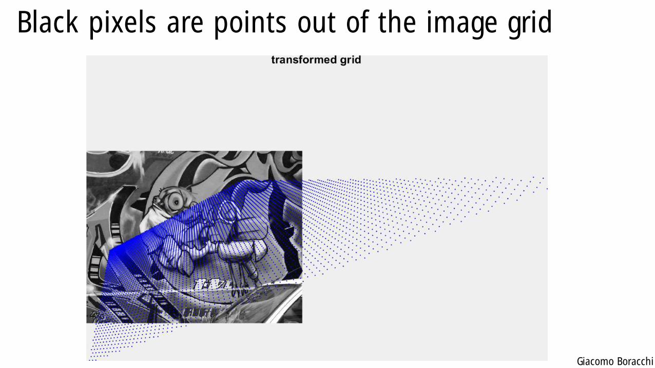
Black pixels are points out of the image grid

Giacomo Boracchi
Single-View GeometryGiacomo Boracchi
March 10th, 2020
USI, Lugano
Book: HZ, chapter 2
Giacomo Boracchi
Outline
• Implications of image calibration
• Camera Center
• Viewing Rays
• Factorization of 𝑀
• Conics and Conic Fitting
• Comments on Error Minimization
• Measuring Angles
• Single View Rectification
Giacomo Boracchi
The Camera Center 𝐶
The 3D coordinates of the center of a camera having matrix 𝑀 ∈ ℝ3,4
satisfy
𝐶 ∈ 𝑅𝑁𝑆(𝑀)
Where 𝑅𝑁𝑆(⋅) denotes the Right Null Space.
Note that when the 𝑅𝑁𝑆(𝑀) has dimension 1 (i.e. always but in
degenerate cases) all the points 𝐶 ∈ 𝑅𝑁𝑆 𝑀 coincide in the
homogenous space.

Giacomo Boracchi
The Camera Center 𝐶
Proof
Let us consider 𝐶 ∈ 𝑅𝑁𝑆(𝑀), then
𝑀𝑃 = 𝑀 𝑃 + 𝜆𝐶 ∀𝜆 ∈ ℝ, ∀𝑃 ∈ ℙ3
This means that the line 𝑃 + 𝜆𝐶 does not change its projection through
𝑀, thus 𝑃 + 𝜆𝐶 is a viewing ray. Since this has to hold ∀𝑃 ∈ ℙ3, this
means that 𝐶 is the camera center.
The converse is trivial because given the camera center 𝐶, then
𝑀 𝑃 + 𝜆𝐶 = 𝑀𝑃 ∀𝑃 ∈ ℙ3 (since 𝑃 + 𝜆𝐶 is homogeneous coordinates
is the viewing ray), thus 𝐶 ∈ 𝑅𝑁𝑆(𝑀)
Giacomo Boracchi
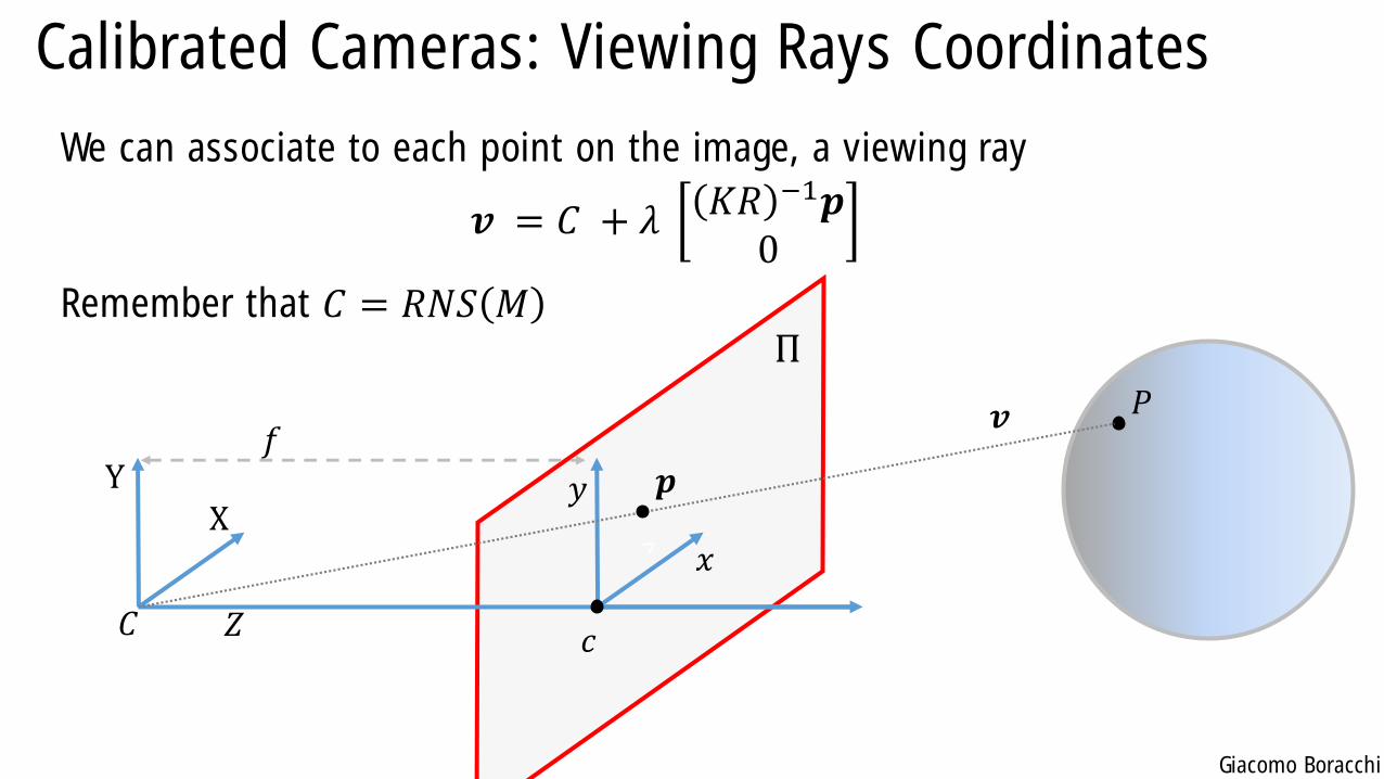
Calibrated Cameras: Viewing Rays Coordinates
We can associate to each point on the image, a viewing ray
𝒗 = 𝐶 + 𝜆 𝐾𝑅 −1𝒑0
Remember that 𝐶 = 𝑅𝑁𝑆 𝑀
XY
𝑍𝐶
Π
𝑐
𝑓
𝑥
𝑦
𝑃
𝒑
𝒗
Giacomo Boracchi
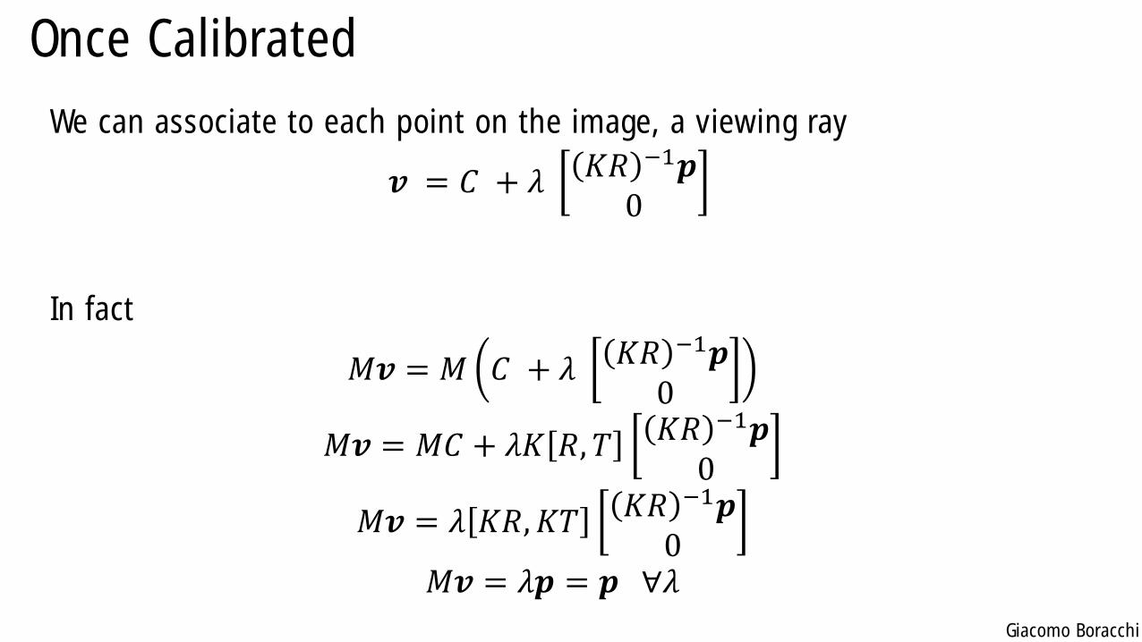
Once Calibrated
We can associate to each point on the image, a viewing ray
𝒗 = 𝐶 + 𝜆 𝐾𝑅 −1𝒑0
In fact
𝑀𝒗 = 𝑀 𝐶 + 𝜆 𝐾𝑅 −1𝒑0
𝑀𝒗 = 𝑀𝐶 + 𝜆𝐾 𝑅, 𝑇 𝐾𝑅 −1𝒑0
𝑀𝒗 = 𝜆 𝐾𝑅,𝐾𝑇 𝐾𝑅 −1𝒑0
𝑀𝒗 = 𝜆𝒑 = 𝒑 ∀𝜆
Giacomo Boracchi
Once Calibrated: Factorization of 𝑀
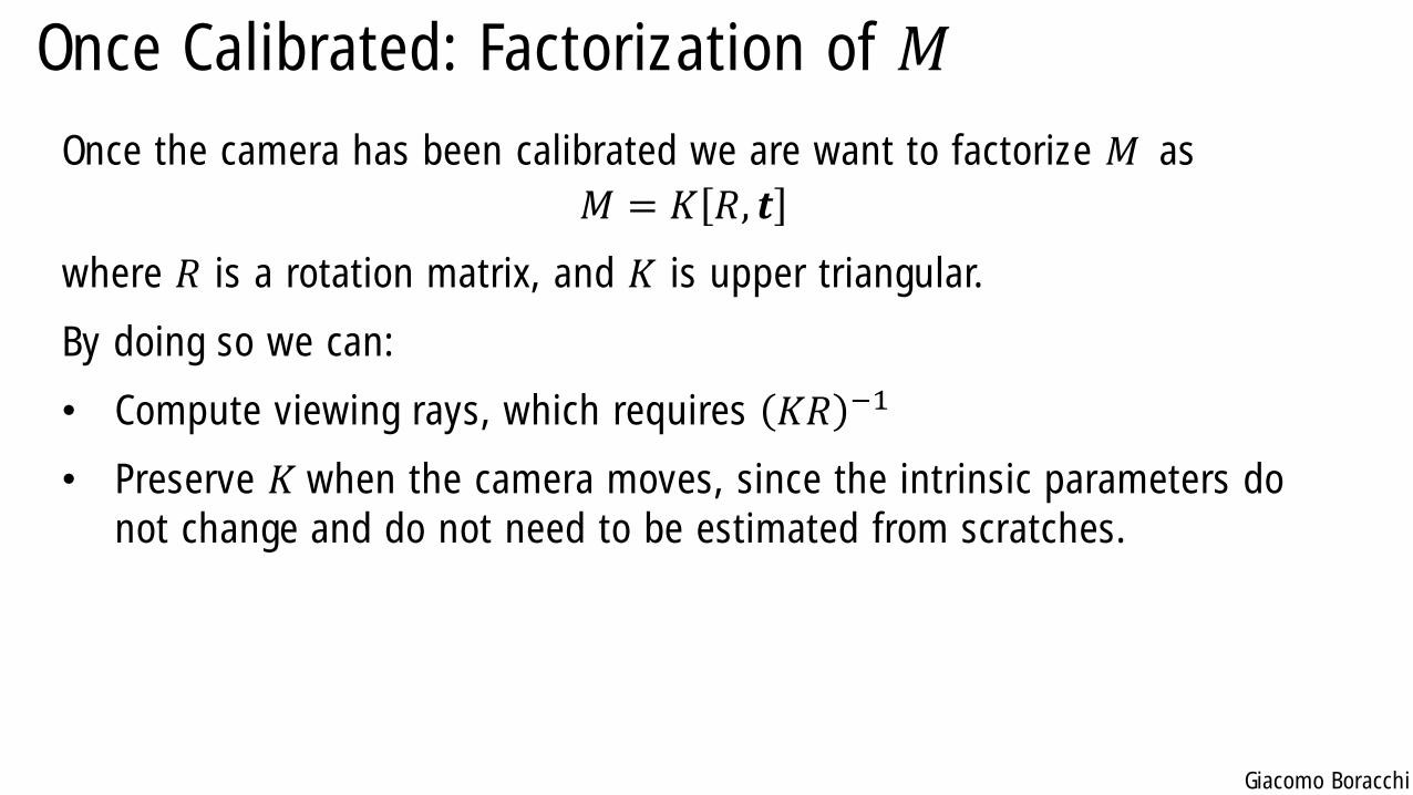
Once the camera has been calibrated we are want to factorize 𝑀 as
𝑀 = 𝐾 𝑅, 𝒕
where 𝑅 is a rotation matrix, and 𝐾 is upper triangular.
By doing so we can:
• Compute viewing rays, which requires 𝐾𝑅 −1
• Preserve 𝐾 when the camera moves, since the intrinsic parameters do
not change and do not need to be estimated from scratches.
Giacomo Boracchi
Factorization of 𝑀
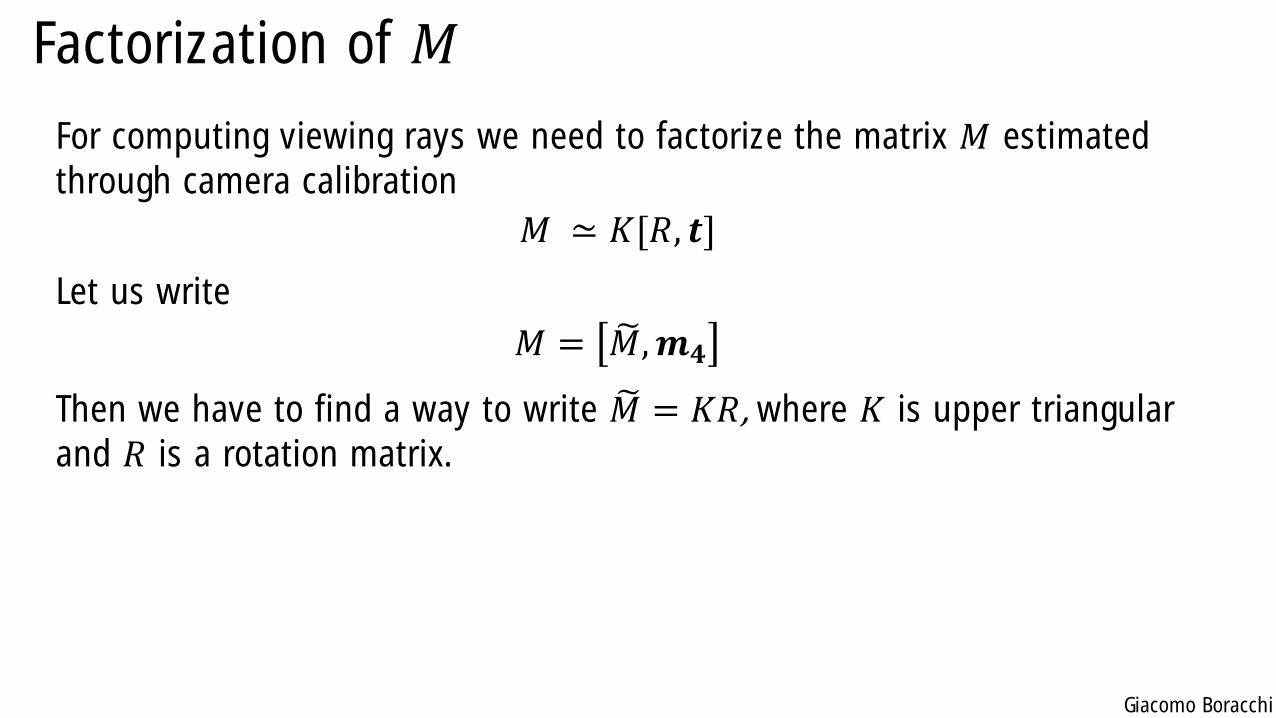
For computing viewing rays we need to factorize the matrix 𝑀 estimated
through camera calibration
𝑀 ≃ 𝐾[𝑅, 𝒕]
Let us write
𝑀 = ෩𝑀,𝒎𝟒
Then we have to find a way to write ෩𝑀 = 𝐾𝑅, where 𝐾 is upper triangular
and 𝑅 is a rotation matrix.
Giacomo Boracchi
Factorization of 𝑀
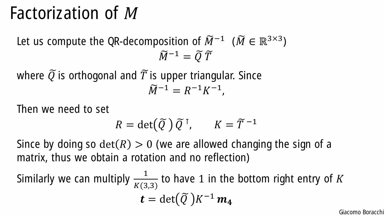
Let us compute the QR-decomposition of ෩𝑀−1 ( ෩𝑀 ∈ ℝ3×3)
෩𝑀−1 = ෩𝑄 ෩𝑇
where ෩𝑄 is orthogonal and ෩𝑇 is upper triangular. Since
෩𝑀−1 = 𝑅−1𝐾−1,
Then we need to set
𝑅 = det ෩𝑄 ෩𝑄 ⊺, 𝐾 = ෩𝑇 −1
Since by doing so det 𝑅 > 0 (we are allowed changing the sign of a
matrix, thus we obtain a rotation and no reflection)
Similarly we can multiply 1
𝐾(3,3)to have 1 in the bottom right entry of 𝐾
𝒕 = det ෩𝑄 𝐾−1𝒎𝟒
Giacomo Boracchi
Factorization of 𝑀
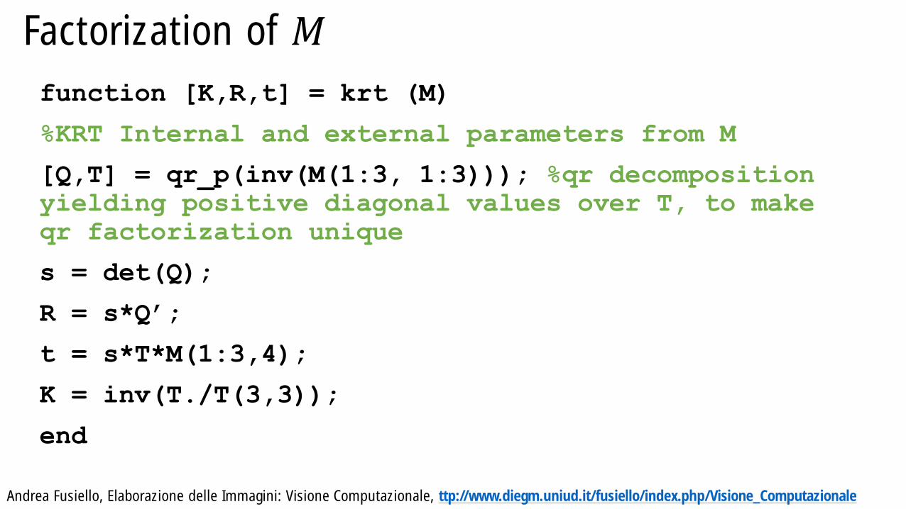
function [K,R,t] = krt (M)
%KRT Internal and external parameters from M
[Q,T] = qr_p(inv(M(1:3, 1:3))); %qr decomposition
yielding positive diagonal values over T, to make
qr factorization unique
s = det(Q);
R = s*Q’;
t = s*T*M(1:3,4);
K = inv(T./T(3,3));
end
Andrea Fusiello, Elaborazione delle Immagini: Visione Computazionale, ttp://www.diegm.uniud.it/fusiello/index.php/Visione_Computazionale
Giacomo Boracchi
A recap on Camera Projection
Giacomo Boracchi
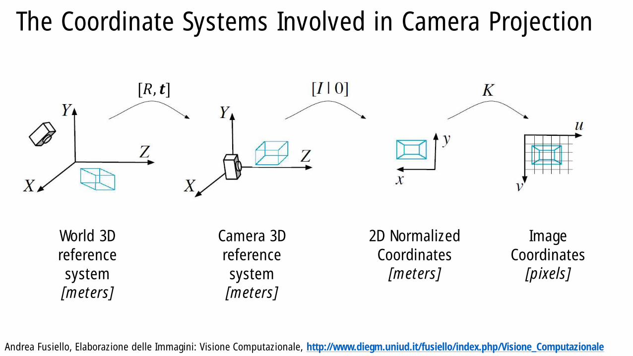
The Coordinate Systems Involved in Camera Projection
Andrea Fusiello, Elaborazione delle Immagini: Visione Computazionale, http://www.diegm.uniud.it/fusiello/index.php/Visione_Computazionale
[𝑅, 𝒕]
World 3D
reference
system
[meters]
Camera 3D
reference
system
[meters]
2D Normalized
Coordinates
[meters]
Image
Coordinates
[pixels]
Giacomo Boracchi
Conics
Giacomo Boracchi
Conics
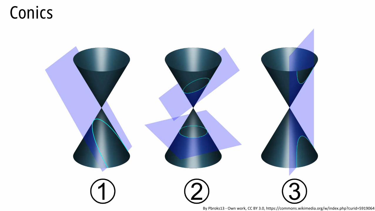
By Pbroks13 - Own work, CC BY 3.0, https://commons.wikimedia.org/w/index.php?curid=5919064
Giacomo Boracchi
Conics in ℙ2
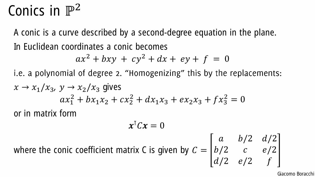
A conic is a curve described by a second-degree equation in the plane.
In Euclidean coordinates a conic becomes
𝑎𝑥2 + 𝑏𝑥𝑦 + 𝑐𝑦2 + 𝑑𝑥 + 𝑒𝑦 + 𝑓 = 0
𝑥 → 𝑥1/𝑥3, 𝑦 → 𝑥2/𝑥3 gives
𝑎𝑥12 + 𝑏𝑥1𝑥2 + 𝑐𝑥2
2 + 𝑑𝑥1𝑥3 + 𝑒𝑥2𝑥3 + 𝑓𝑥32 = 0
or in matrix form
𝒙⊺𝐶𝒙 = 0
where the conic coefficient matrix C is given by 𝐶 =
𝑎 𝑏/2 𝑑/2𝑏/2 𝑐 𝑒/2𝑑/2 𝑒/2 𝑓
Giacomo Boracchi
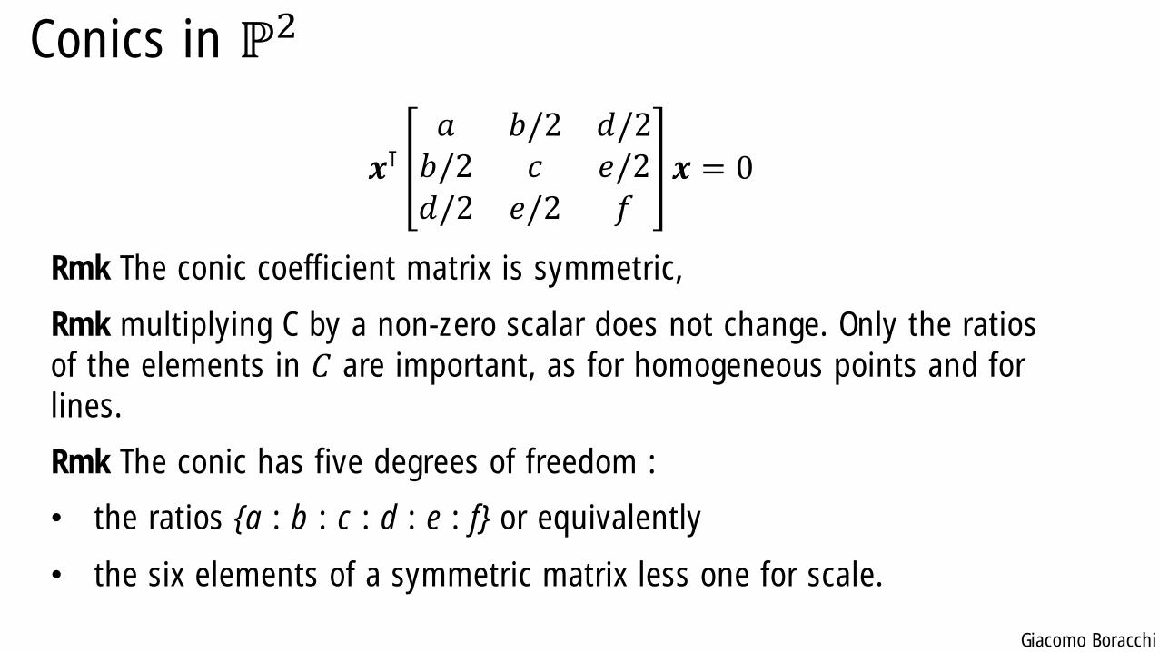
Conics in ℙ2
𝒙⊺𝑎 𝑏/2 𝑑/2𝑏/2 𝑐 𝑒/2𝑑/2 𝑒/2 𝑓
𝒙 = 0
Rmk The conic coefficient matrix is symmetric,
Rmk multiplying C by a non-zero scalar does not change. Only the ratios
of the elements in 𝐶 are important, as for homogeneous points and for
lines.
Rmk The conic has five degrees of freedom :
• the ratios {a : b : c : d : e : f} or equivalently
• the six elements of a symmetric matrix less one for scale.

Giacomo Boracchi
Conic Fitting
Giacomo Boracchi
Conic fitting
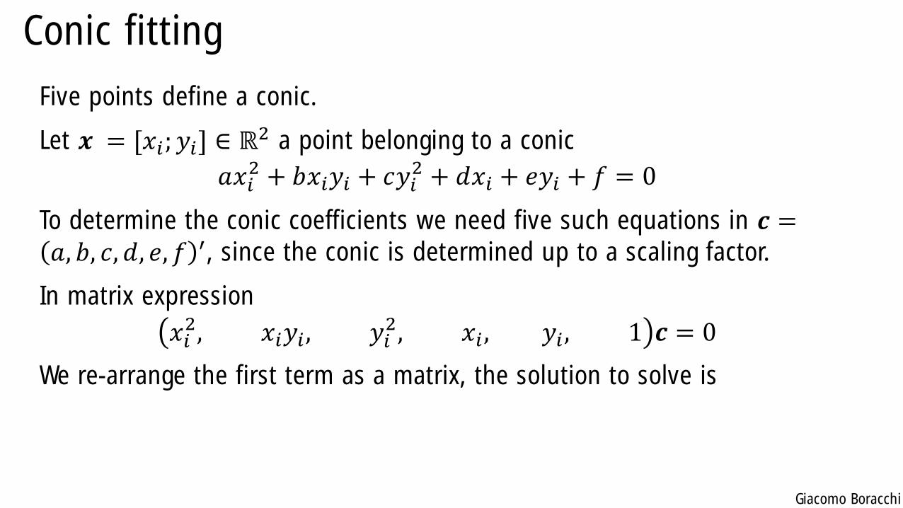
Five points define a conic.
Let 𝒙 = [𝑥𝑖; 𝑦𝑖] ∈ ℝ2 a point belonging to a conic
𝑎𝑥𝑖2 + 𝑏𝑥𝑖𝑦𝑖 + 𝑐𝑦𝑖
2 + 𝑑𝑥𝑖 + 𝑒𝑦𝑖 + 𝑓 = 0
To determine the conic coefficients we need five such equations in 𝒄 =𝑎, 𝑏, 𝑐, 𝑑, 𝑒, 𝑓 ′, since the conic is determined up to a scaling factor.
In matrix expression
𝑥𝑖2, 𝑥𝑖𝑦𝑖 , 𝑦𝑖
2, 𝑥𝑖 , 𝑦𝑖 , 1 𝒄 = 0
We re-arrange the first term as a matrix, the solution to solve is
Giacomo Boracchi
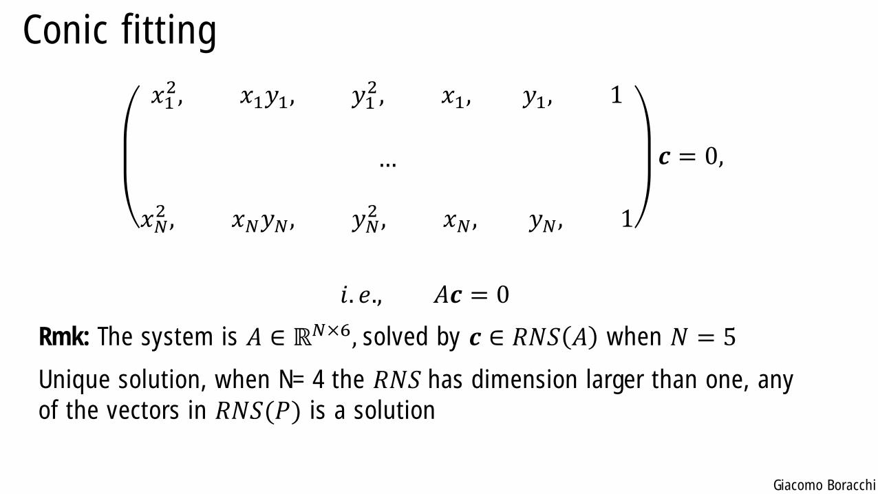
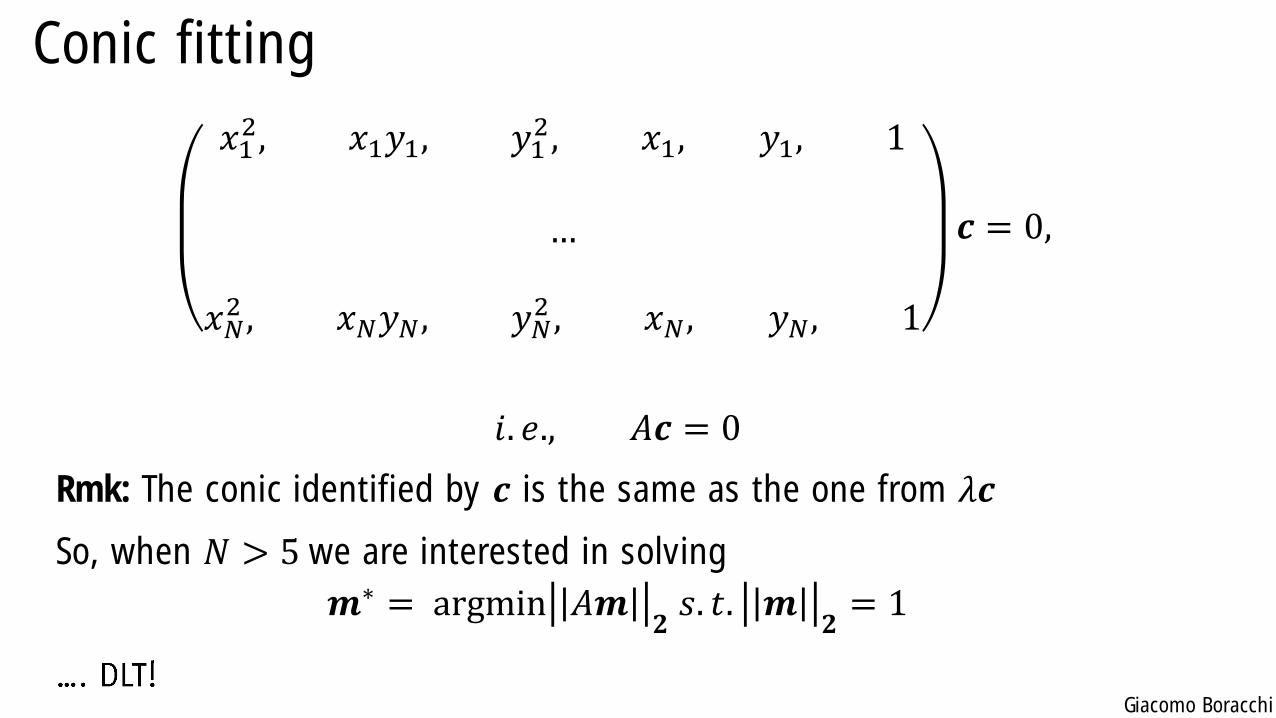
Conic fitting
𝑥12, 𝑥1𝑦1, 𝑦1
2, 𝑥1, 𝑦1, 1
…
𝑥𝑁2 , 𝑥𝑁𝑦𝑁, 𝑦𝑁
2 , 𝑥𝑁, 𝑦𝑁, 1
𝒄 = 0,
𝑖. 𝑒., 𝐴𝒄 = 0
Rmk: The system is 𝐴 ∈ ℝ𝑁×6, solved by 𝒄 ∈ 𝑅𝑁𝑆 𝐴 when 𝑁 = 5
Unique solution, when N= 4 the 𝑅𝑁𝑆 has dimension larger than one, any
of the vectors in 𝑅𝑁𝑆(𝑃) is a solution
Giacomo Boracchi
Conic fitting
𝑥12, 𝑥1𝑦1, 𝑦1
2, 𝑥1, 𝑦1, 1
…
𝑥𝑁2 , 𝑥𝑁𝑦𝑁, 𝑦𝑁
2 , 𝑥𝑁, 𝑦𝑁, 1
𝒄 = 0,
𝑖. 𝑒., 𝐴𝒄 = 0
Rmk: The conic identified by 𝒄 is the same as the one from 𝜆𝒄
So, when 𝑁 > 5 we are interested in solving
𝒎∗ = argmin 𝐴𝒎𝟐𝑠. 𝑡. 𝒎
𝟐= 1
Giacomo Boracchi
Lines tangent to a conic
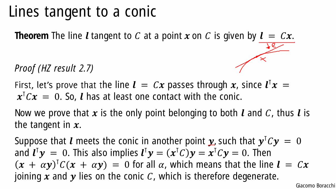
Theorem The line 𝒍 tangent to 𝐶 at a point 𝒙 on 𝐶 is given by 𝒍 = 𝐶𝒙.
Proof (HZ result 2.7)
he line 𝒍 = 𝐶𝒙 passes through 𝒙, since 𝒍⊺𝒙 =𝒙⊺𝐶𝒙 = 0. So, 𝒍 has at least one contact with the conic.
Now we prove that 𝒙 is the only point belonging to both 𝒍 and 𝐶, thus 𝒍 is
the tangent in 𝒙.
Suppose that 𝒍 meets the conic in another point 𝒚, such that 𝒚⊺𝐶𝒚 = 0and 𝒍⊺𝒚 = 0. This also implies 𝒍⊺𝒚 = 𝒙⊺𝐶 𝒚 = 𝒙⊺𝐶𝒚 = 0. Then
𝒙 + 𝛼𝒚 ⊺𝐶(𝒙 + 𝛼𝒚) = 0 for all 𝛼, which means that the line 𝒍 = 𝐶𝒙joining 𝒙 and 𝒚 lies on the conic 𝐶, which is therefore degenerate.

Giacomo Boracchi
Matlab Example
Giacomo Boracchi
Comments on Error Minimization
Giacomo Boracchi
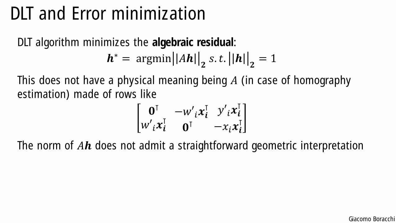
DLT and Error minimization
DLT algorithm minimizes the algebraic residual:
𝒉∗ = argmin 𝐴𝒉𝟐𝑠. 𝑡. 𝒉
𝟐= 1
This does not have a physical meaning being 𝐴 (in case of homography
estimation) made of rows like
𝟎⊺
𝑤′𝑖𝒙𝒊⊺−𝑤′𝑖𝒙𝒊
⊺
𝟎⊺𝑦′𝑖𝒙𝒊
⊺
−𝑥𝑖𝒙𝒊⊺
The norm of 𝐴𝒉 does not admit a straightforward geometric interpretation
Giacomo Boracchi
DLT and Error minimization
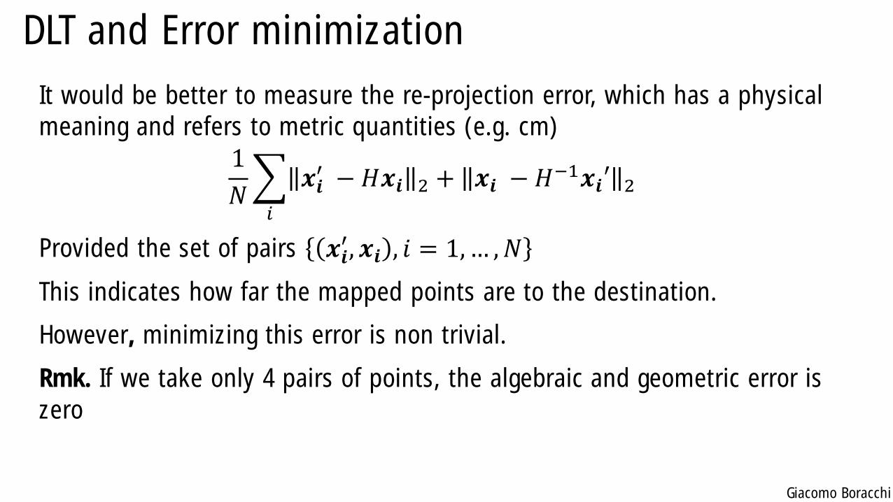
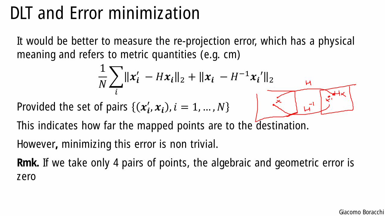
It would be better to measure the re-projection error, which has a physical
meaning and refers to metric quantities (e.g. cm)
1
𝑁
𝑖
𝒙𝒊′ −𝐻𝒙𝒊 2 + 𝒙𝒊 −𝐻−1𝒙𝒊′ 2
Provided the set of pairs 𝒙𝒊′, 𝒙𝒊 , 𝑖 = 1,… ,𝑁
This indicates how far the mapped points are to the destination.
However, minimizing this error is non trivial.
Rmk. If we take only 4 pairs of points, the algebraic and geometric error is
zero
Giacomo Boracchi
DLT and Error minimization
It would be better to measure the re-projection error, which has a physical
meaning and refers to metric quantities (e.g. cm)
1
𝑁
𝑖
𝒙𝒊′ −𝐻𝒙𝒊 2 + 𝒙𝒊 −𝐻−1𝒙𝒊′ 2
Provided the set of pairs 𝒙𝒊′, 𝒙𝒊 , 𝑖 = 1,… ,𝑁
This indicates how far the mapped points are to the destination.
However, minimizing this error is non trivial.
Rmk. If we take only 4 pairs of points, the algebraic and geometric error is
zero
Giacomo Boracchi
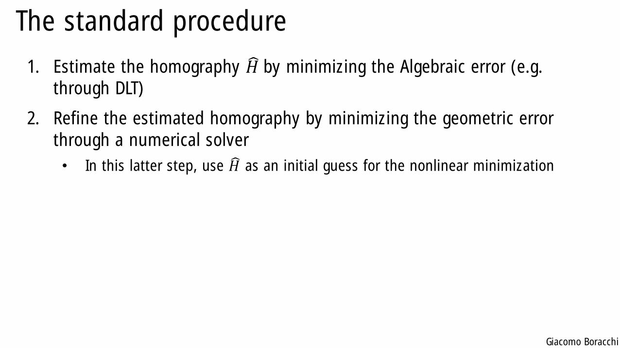
The standard procedure
1. Estimate the homography 𝐻 by minimizing the Algebraic error (e.g.
through DLT)
2. Refine the estimated homography by minimizing the geometric error
through a numerical solver
• In this latter step, use 𝐻 as an initial guess for the nonlinear minimization
Giacomo Boracchi
Dual Conic
Giacomo Boracchi
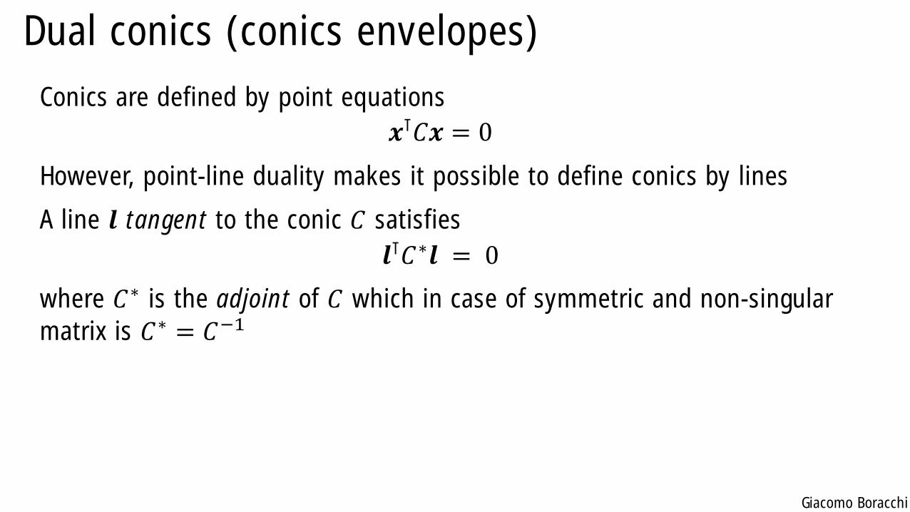
Dual conics (conics envelopes)
Conics are defined by point equations
𝒙⊺𝐶𝒙 = 0
However, point-line duality makes it possible to define conics by lines
A line 𝒍 tangent to the conic 𝐶 satisfies
𝒍⊺𝐶∗𝒍 = 0
where 𝐶∗ is the adjoint of 𝐶 which in case of symmetric and non-singular
matrix is 𝐶∗ = 𝐶−1
Giacomo Boracchi
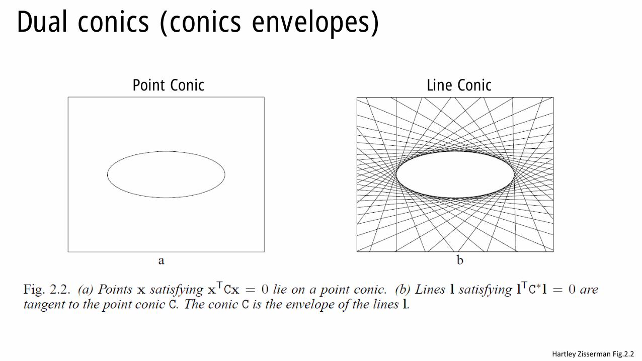
Dual conics (conics envelopes)
Hartley Zisserman Fig.2.2
Point Conic Line Conic
Giacomo Boracchi
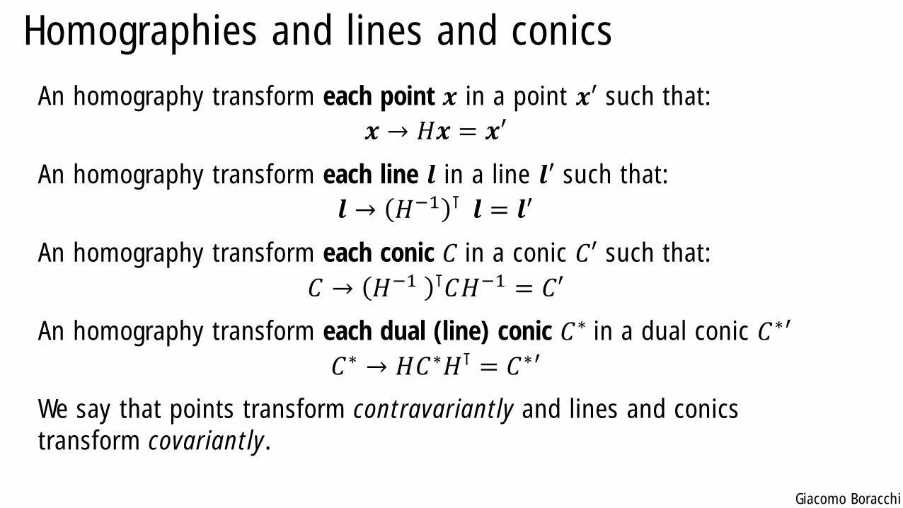
Homographies and lines and conics
An homography transform each point 𝒙 in a point 𝒙′ such that:
𝒙 → 𝐻𝒙 = 𝒙′
An homography transform each line 𝒍 in a line 𝒍′ such that:
𝒍 → 𝐻−1 ⊺ 𝒍 = 𝒍′
An homography transform each conic 𝐶 in a conic 𝐶′ such that:
𝐶 → 𝐻−1 ⊺𝐶𝐻−1 = 𝐶′
An homography transform each dual (line) conic 𝐶∗ in a dual conic 𝐶∗′
𝐶∗ → 𝐻𝐶∗𝐻⊺ = 𝐶∗′
We say that points transform contravariantly and lines and conics
transform covariantly.
Giacomo Boracchi
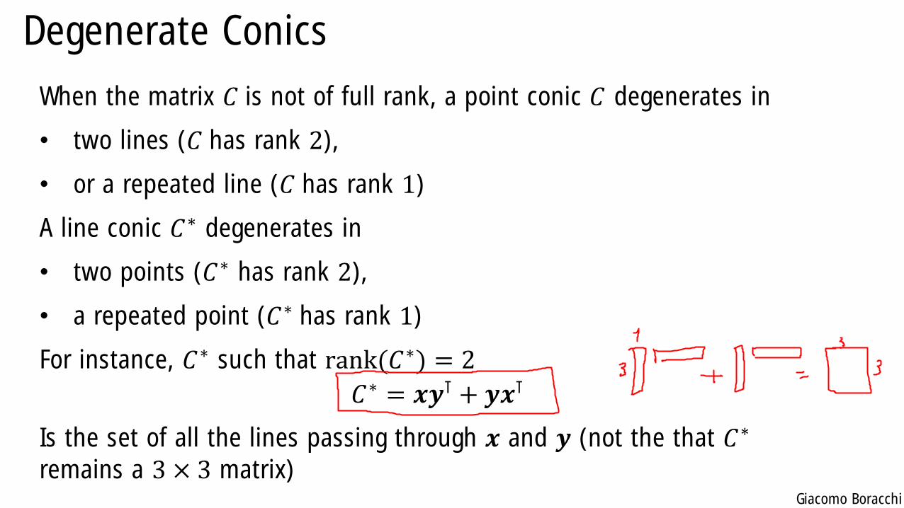
Degenerate Conics
When the matrix 𝐶 is not of full rank, a point conic 𝐶 degenerates in
• two lines (𝐶 has rank 2),
• or a repeated line (𝐶 has rank 1)
A line conic 𝐶∗ degenerates in
• two points (𝐶∗ has rank 2),
• a repeated point (𝐶∗ has rank 1)
For instance, 𝐶∗ such that rank(𝐶∗) = 2
𝐶∗ = 𝒙𝒚⊺ + 𝒚𝒙⊺
Is the set of all the lines passing through 𝒙 and 𝒚 (not the that 𝐶∗
remains a 3 × 3 matrix)
Giacomo Boracchi
Circular Points and Conic dual to circular points
Giacomo Boracchi
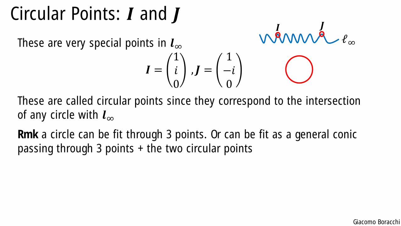
Circular Points: 𝑰 and 𝑱
These are very special points in 𝒍∞
𝑰 =1𝑖0
, 𝑱 =1−𝑖0
These are called circular points since they correspond to the intersection
of any circle with 𝒍∞
Rmk a circle can be fit through 3 points. Or can be fit as a general conic
passing through 3 points + the two circular points
ℓ∞
𝑱𝑰
Giacomo Boracchi
Circular Points: 𝑰 and 𝑱
Circular points are fixed under an orientation-preserving similarity
𝐻𝑆𝑰 = 𝑰, 𝐻𝑆𝑱 = 𝑱
a reflection instead swaps 𝑰 and 𝑱
Rmk circular points are not fixed under projective transformations
Giacomo Boracchi
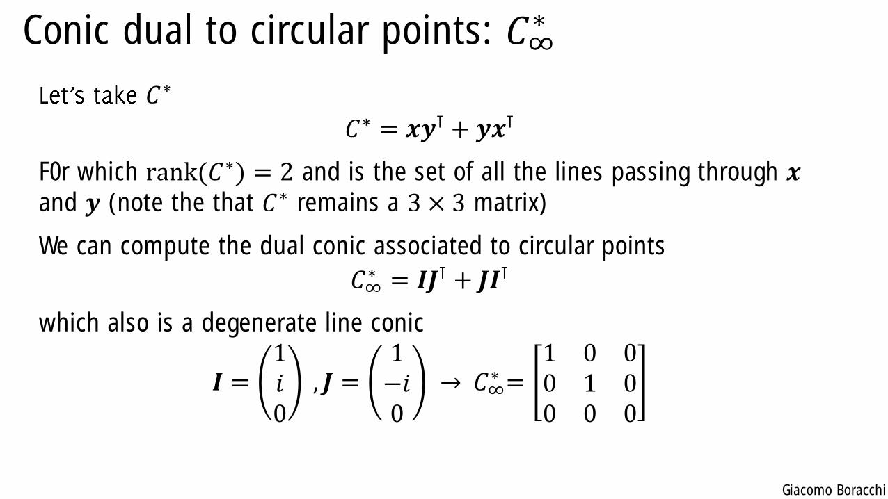
Conic dual to circular points: 𝐶∞∗
𝐶∗
𝐶∗ = 𝒙𝒚⊺ + 𝒚𝒙⊺
F0r which rank(𝐶∗) = 2 and is the set of all the lines passing through 𝒙and 𝒚 (note the that 𝐶∗ remains a 3 × 3 matrix)
We can compute the dual conic associated to circular points
𝐶∞∗ = 𝑰𝑱⊺ + 𝑱𝑰⊺
which also is a degenerate line conic
𝑰 =1𝑖0
, 𝑱 =1−𝑖0
→ 𝐶∞∗ =
1 0 00 1 00 0 0
Giacomo Boracchi
Conic dual to circular points: 𝐶∞∗
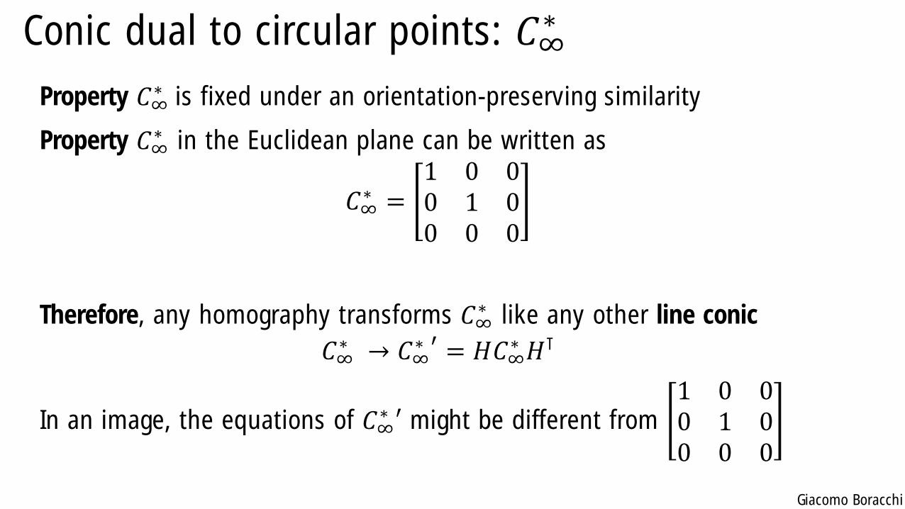
Property 𝐶∞∗ is fixed under an orientation-preserving similarity
Property 𝐶∞∗ in the Euclidean plane can be written as
𝐶∞∗ =
1 0 00 1 00 0 0
Therefore, any homography transforms 𝐶∞∗ like any other line conic
𝐶∞∗ → 𝐶∞
∗ ′ = 𝐻𝐶∞∗ 𝐻⊺
In an image, the equations of 𝐶∞∗ ′ might be different from
1 0 00 1 00 0 0
Giacomo Boracchi
Single Image Rectification From 𝐶∞∗
Giacomo Boracchi
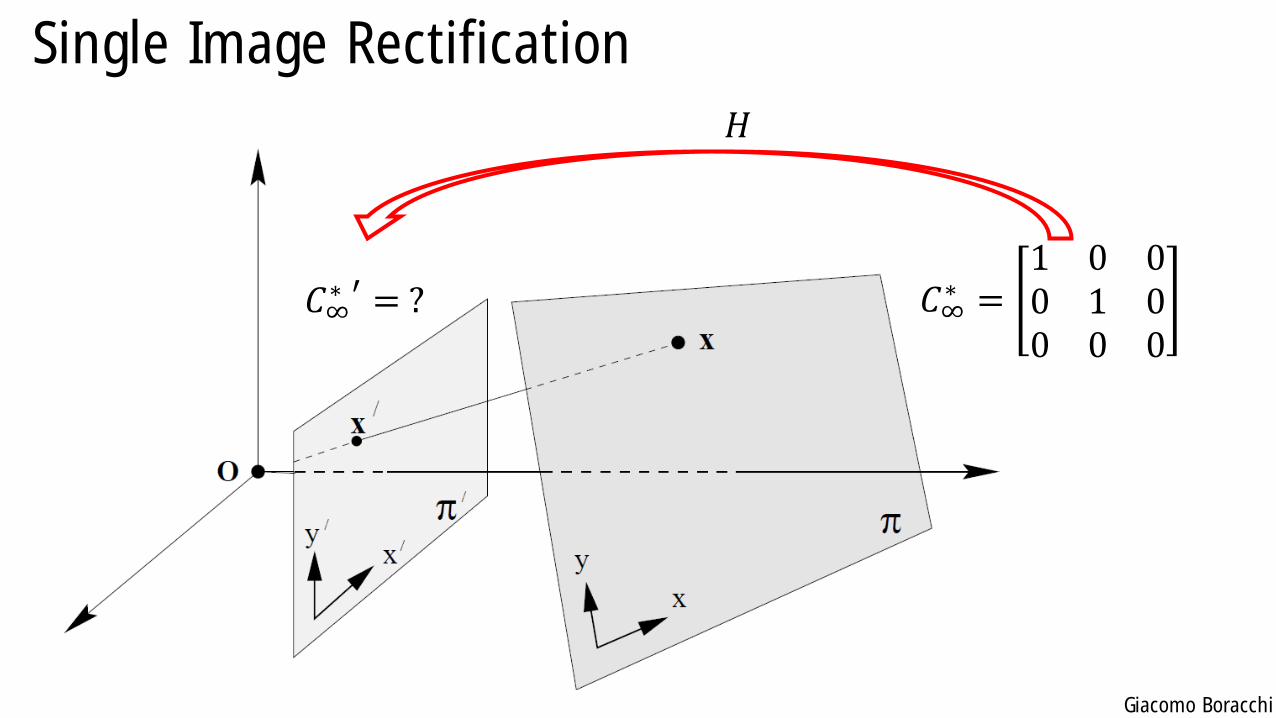
Single Image Rectification
𝐶∞∗ =
1 0 00 1 00 0 0
𝐶∞∗ ′ = ?
𝐻
Giacomo Boracchi
Single Image Rectification
𝐶∞∗ =
1 0 00 1 00 0 0
𝐶∞∗ ′ = ?
𝐻
Giacomo Boracchi
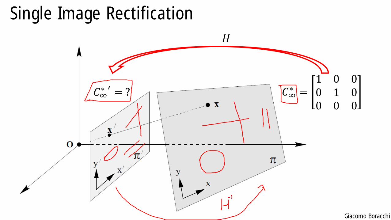
Single Image Rectification
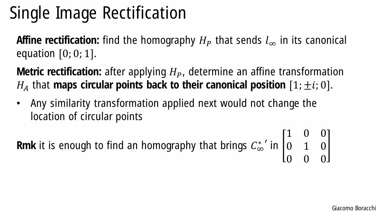
Affine rectification: find the homography 𝐻𝑃 that sends 𝑙∞ in its canonical
equation [0; 0; 1].
Metric rectification: after applying 𝐻𝑃, determine an affine transformation
𝐻𝐴 that maps circular points back to their canonical position [1;±𝑖; 0].
• Any similarity transformation applied next would not change the
location of circular points
Rmk it is enough to find an homography that brings 𝐶∞∗ ′ in
1 0 00 1 00 0 0
Giacomo Boracchi
Single Image Rectification
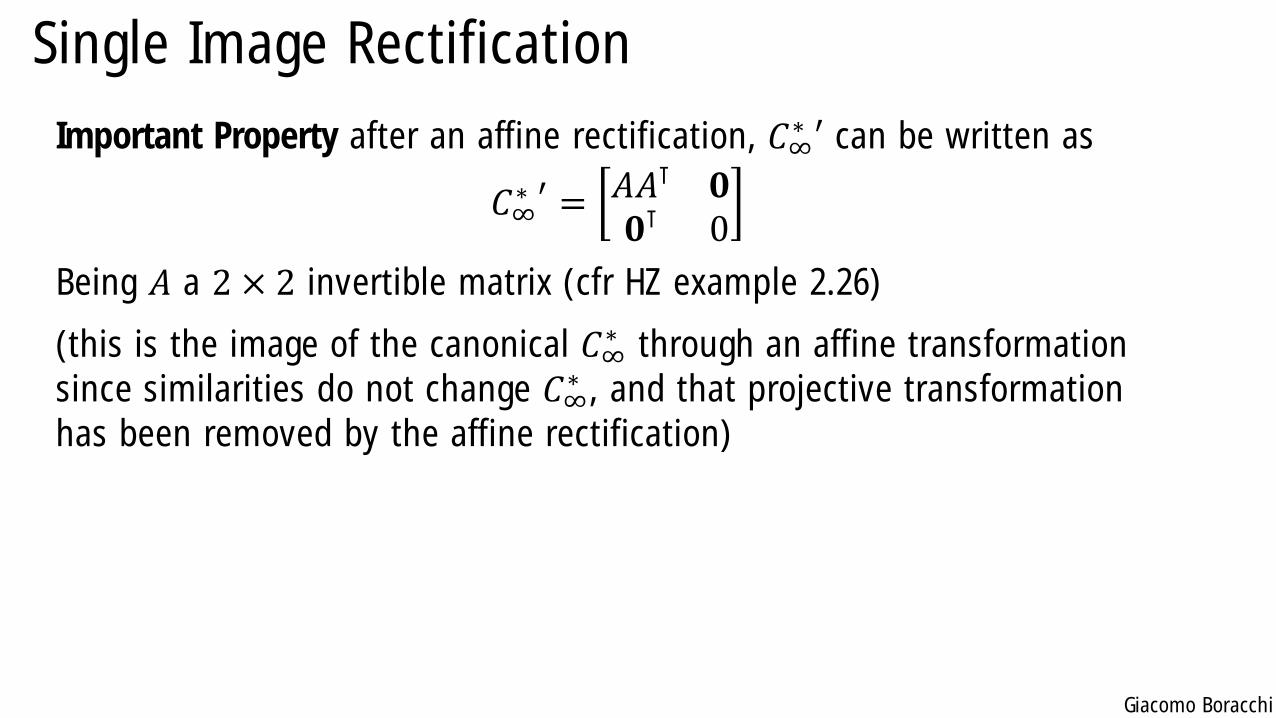
Important Property after an affine rectification, 𝐶∞∗ ′ can be written as
𝐶∞∗ ′ = 𝐴𝐴⊺ 𝟎
𝟎⊺ 0
Being 𝐴 a 2 × 2 invertible matrix (cfr HZ example 2.26)
(this is the image of the canonical 𝐶∞∗ through an affine transformation
since similarities do not change 𝐶∞∗ , and that projective transformation
has been removed by the affine rectification)

Giacomo Boracchi
Single Image Rectification (after affine rectification)
Our goal is to estimate that 𝐻 in order to define the inverse mapping 𝐻−1
Assume now that that affine rectification has been already performed
𝐶∞∗ =
1 0 00 1 00 0 0
𝐶∞∗ ′ = 𝐴𝐴⊺ 𝟎
𝟎⊺ 0
𝐻
Giacomo Boracchi
Single Image Rectification
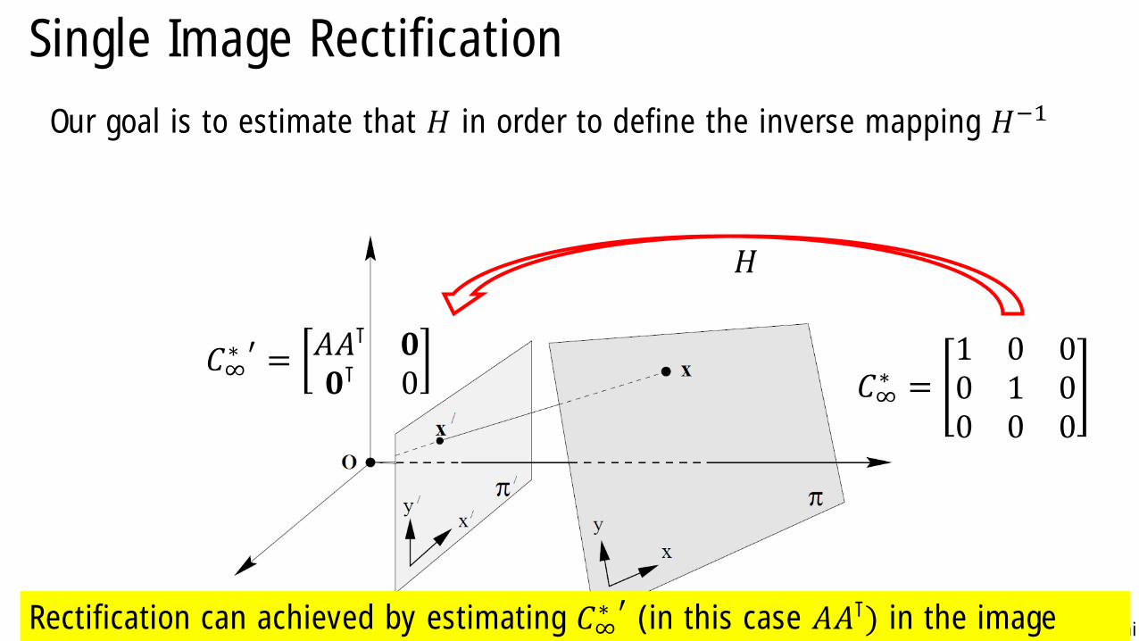
Our goal is to estimate that 𝐻 in order to define the inverse mapping 𝐻−1
𝐶∞∗ =
1 0 00 1 00 0 0
Rectification can achieved by estimating 𝐶∞∗ ′ (in this case 𝐴𝐴⊺) in the image
𝐶∞∗ ′ = 𝐴𝐴⊺ 𝟎
𝟎⊺ 0
𝐻
Giacomo Boracchi
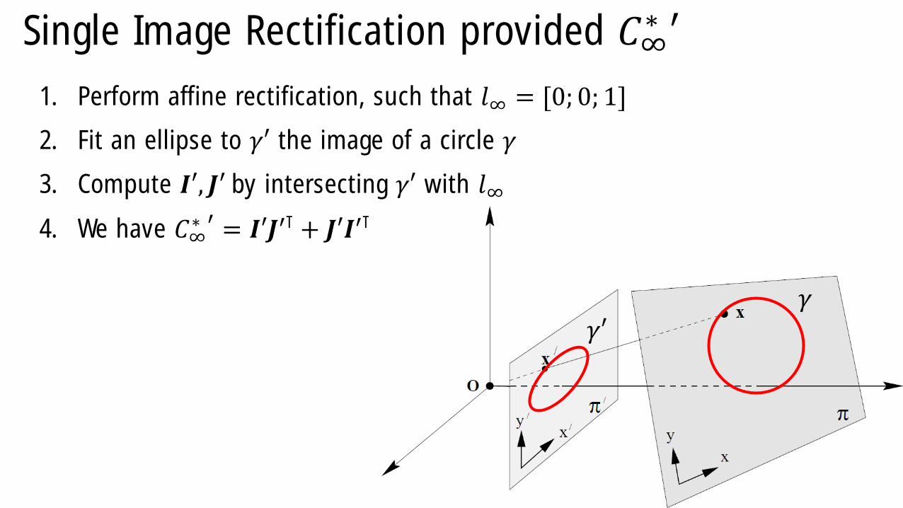
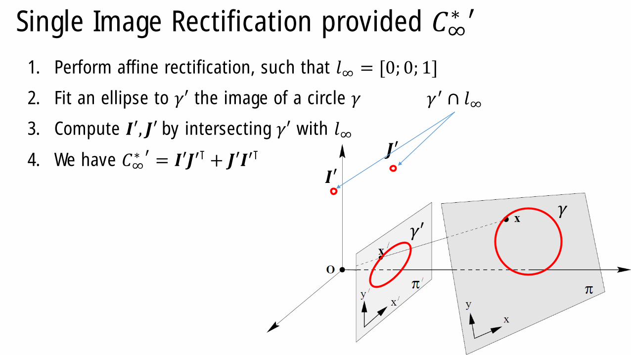
Single Image Rectification provided 𝐶∞∗ ′
1. Perform affine rectification, such that 𝑙∞ = [0; 0; 1]
2. Fit an ellipse to 𝛾′ the image of a circle 𝛾
3. Compute 𝑰′, 𝑱′ by intersecting 𝛾′ with 𝑙∞
4. We have 𝐶∞∗ ′ = 𝑰′𝑱′⊺ + 𝑱′𝑰′⊺
𝛾𝛾′
Giacomo Boracchi
Single Image Rectification provided 𝐶∞∗ ′
1. Perform affine rectification, such that 𝑙∞ = [0; 0; 1]
2. Fit an ellipse to 𝛾′ the image of a circle 𝛾
3. Compute 𝑰′, 𝑱′ by intersecting 𝛾′ with 𝑙∞
4. We have 𝐶∞∗ ′ = 𝑰′𝑱′⊺ + 𝑱′𝑰′⊺
𝛾𝛾′
𝛾′ ∩ 𝑙∞
𝑰′
𝑱′
Giacomo Boracchi
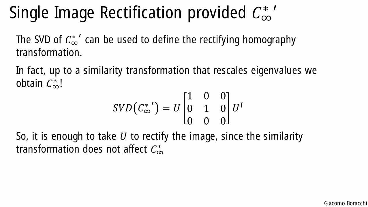
Single Image Rectification provided 𝐶∞∗ ′
The SVD of 𝐶∞∗ ′ can be used to define the rectifying homography
transformation.
In fact, up to a similarity transformation that rescales eigenvalues we
obtain 𝐶∞∗ !
𝑆𝑉𝐷 𝐶∞∗ ′ = 𝑈
1 0 00 1 00 0 0
𝑈⊺
So, it is enough to take 𝑈 to rectify the image, since the similarity
transformation does not affect 𝐶∞∗
Giacomo Boracchi
Single Image Rectification From OrthogonalLines
Giacomo Boracchi
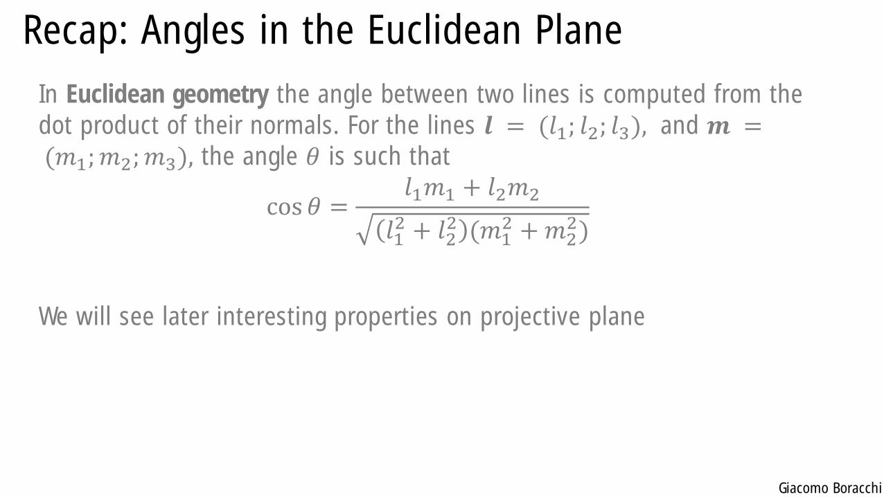
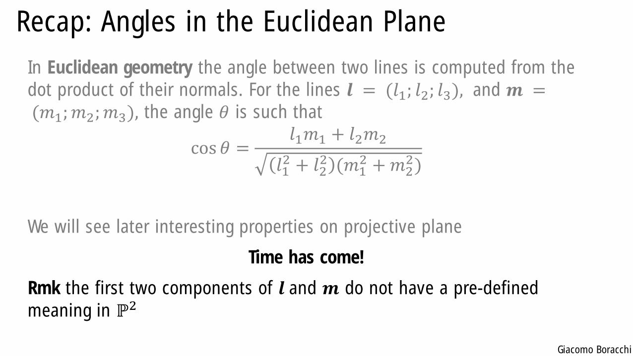
Recap: Angles in the Euclidean Plane
In Euclidean geometry the angle between two lines is computed from the
dot product of their normals. For the lines 𝒍 = (𝑙1; 𝑙2; 𝑙3), and 𝒎 =(𝑚1;𝑚2;𝑚3), the angle 𝜃 is such that
cos 𝜃 =𝑙1𝑚1 + 𝑙2𝑚2
𝑙12 + 𝑙2
2 (𝑚12 +𝑚2
2)
We will see later interesting properties on projective plane
Giacomo Boracchi
Recap: Angles in the Euclidean Plane
In Euclidean geometry the angle between two lines is computed from the
dot product of their normals. For the lines 𝒍 = (𝑙1; 𝑙2; 𝑙3), and 𝒎 =(𝑚1;𝑚2;𝑚3), the angle 𝜃 is such that
cos 𝜃 =𝑙1𝑚1 + 𝑙2𝑚2
𝑙12 + 𝑙2
2 (𝑚12 +𝑚2
2)
We will see later interesting properties on projective plane
Time has come!
Rmk the first two components of 𝒍 and 𝒎 do not have a pre-defined
meaning in ℙ2
Giacomo Boracchi
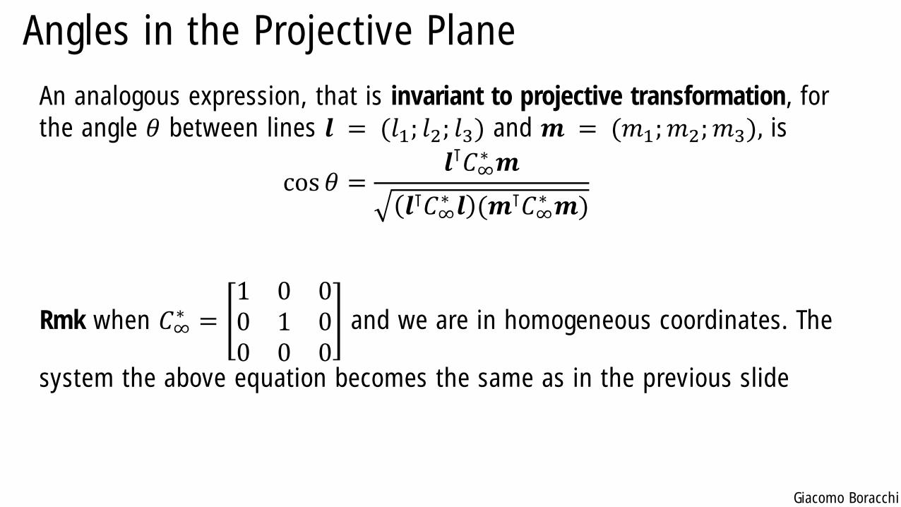
Angles in the Projective Plane
An analogous expression, that is invariant to projective transformation, for
the angle 𝜃 between lines 𝒍 = (𝑙1; 𝑙2; 𝑙3) and 𝒎 = (𝑚1;𝑚2;𝑚3), is
cos 𝜃 =𝒍⊺𝐶∞
∗ 𝒎
𝒍⊺𝐶∞∗ 𝒍 (𝒎⊺𝐶∞
∗ 𝒎)
Rmk when 𝐶∞∗ =
1 0 00 1 00 0 0
and we are in homogeneous coordinates. The
system the above equation becomes the same as in the previous slide
Giacomo Boracchi
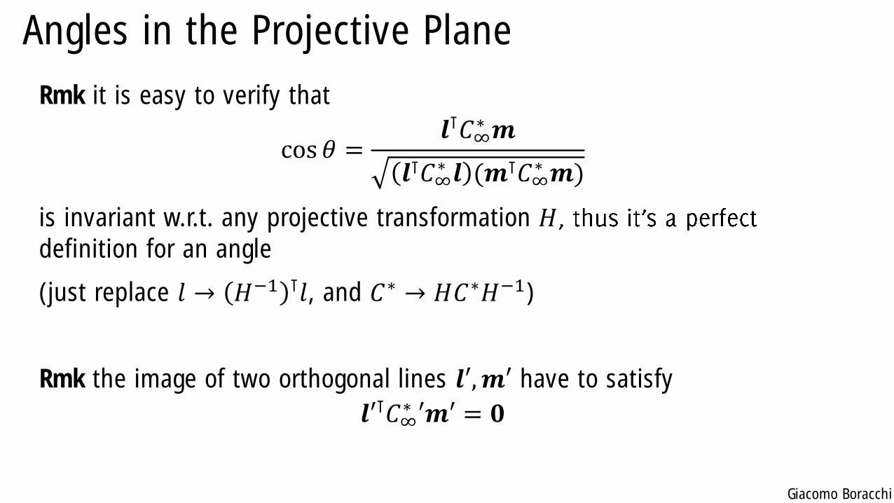
Angles in the Projective Plane
Rmk it is easy to verify that
cos 𝜃 =𝒍⊺𝐶∞
∗ 𝒎
𝒍⊺𝐶∞∗ 𝒍 (𝒎⊺𝐶∞
∗ 𝒎)
is invariant w.r.t. any projective transformation 𝐻definition for an angle
(just replace 𝑙 → 𝐻−1 ⊺𝑙, and 𝐶∗ → 𝐻𝐶∗𝐻−1)
Rmk the image of two orthogonal lines 𝒍′,𝒎′ have to satisfy
𝒍′⊺𝐶∞∗ ′𝒎′ = 𝟎
Giacomo Boracchi
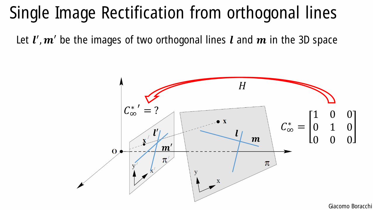
Single Image Rectification from orthogonal lines
𝒍𝒎
𝒍′
𝒎′
Let 𝒍′,𝒎′ be the images of two orthogonal lines 𝒍 and 𝒎 in the 3D space
𝐶∞∗ =
1 0 00 1 00 0 0
𝐶∞∗ ′ = ?
𝐻
Giacomo Boracchi
Single Image Rectification from orthogonal lines
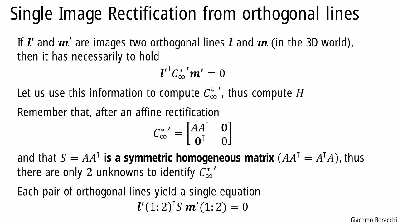
If 𝒍′ and 𝒎′ are images two orthogonal lines 𝒍 and 𝒎 (in the 3D world),
then it has necessarily to hold
𝒍′⊺𝐶∞∗ ′𝒎′ = 0
Let us use this information to compute 𝐶∞∗ ′, thus compute 𝐻
Remember that, after an affine rectification
𝐶∞∗ ′ = 𝐴𝐴⊺ 𝟎
𝟎⊺ 0
and that 𝑆 = 𝐴𝐴⊺ is a symmetric homogeneous matrix 𝐴𝐴⊺ = 𝐴⊺𝐴 , thus
there are only 2 unknowns to identify 𝐶∞∗ ′
Each pair of orthogonal lines yield a single equation
𝒍′ 1: 2 ⊺𝑆 𝒎′(1: 2) = 0
Giacomo Boracchi
Single Image Rectification from orthogonal lines
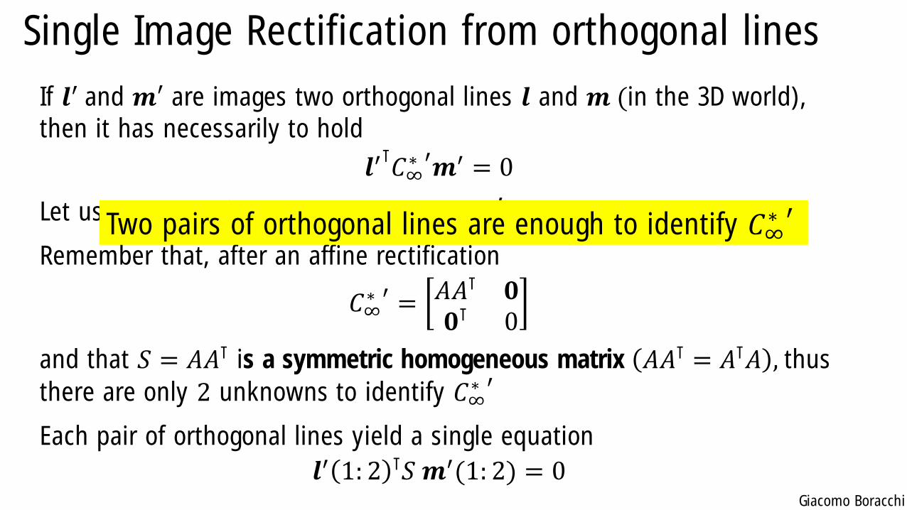
If 𝒍′ and 𝒎′ are images two orthogonal lines 𝒍 and 𝒎 (in the 3D world),
then it has necessarily to hold
𝒍′⊺𝐶∞∗ ′𝒎′ = 0
Let us use this information to compute 𝐶∞∗ ′, thus compute 𝐻
Remember that, after an affine rectification
𝐶∞∗ ′ = 𝐴𝐴⊺ 𝟎
𝟎⊺ 0
and that 𝑆 = 𝐴𝐴⊺ is a symmetric homogeneous matrix 𝐴𝐴⊺ = 𝐴⊺𝐴 , thus
there are only 2 unknowns to identify 𝐶∞∗ ′
Each pair of orthogonal lines yield a single equation
𝒍′ 1: 2 ⊺𝑆 𝒎′(1: 2) = 0
Two pairs of orthogonal lines are enough to identify 𝐶∞∗ ′
Giacomo Boracchi
Stratified Rectification from Orthogonal Lines
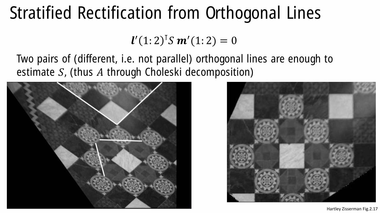
𝒍′ 1: 2 ⊺𝑆 𝒎′(1: 2) = 0
Two pairs of (different, i.e. not parallel) orthogonal lines are enough to
estimate 𝑆, (thus 𝐴 through Choleski decomposition)
Hartley Zisserman Fig.2.17
Giacomo Boracchi
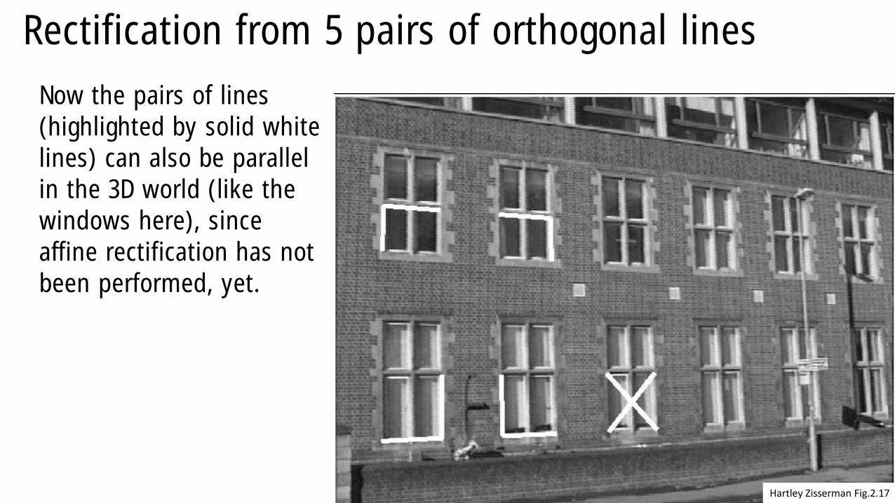
Rectification from 5 pairs of orthogonal lines
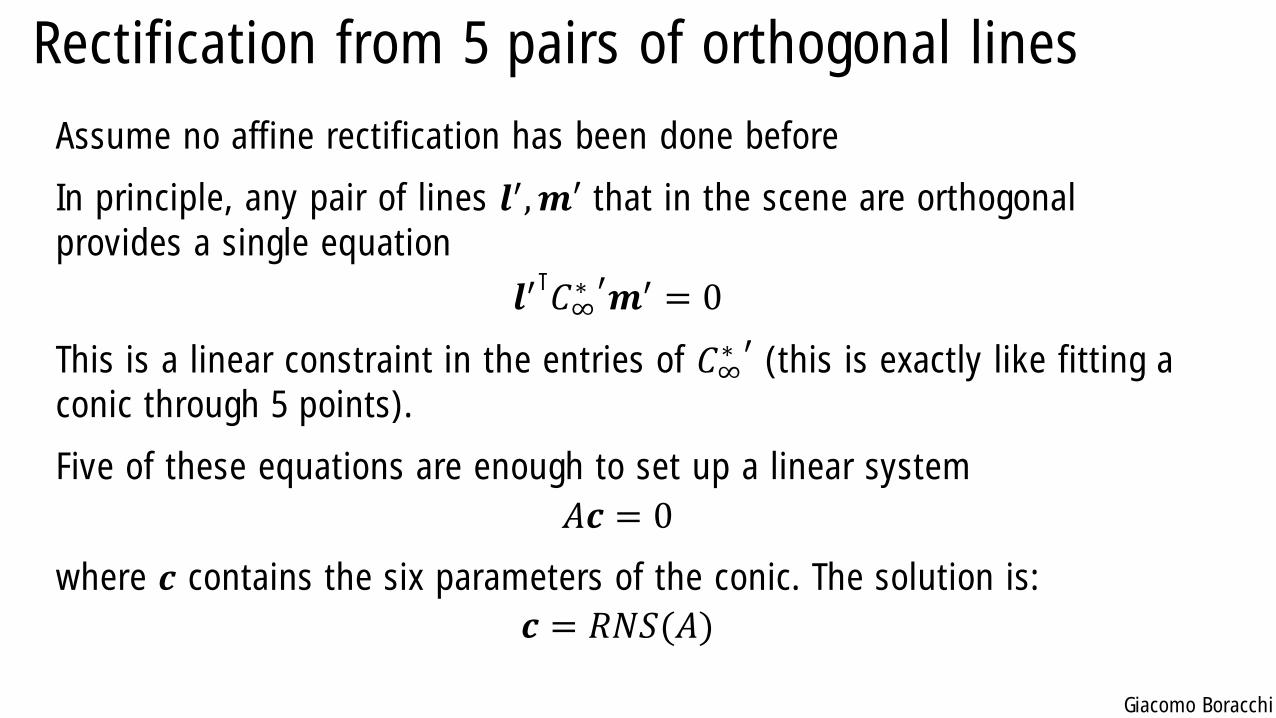
Assume no affine rectification has been done before
In principle, any pair of lines 𝒍′,𝒎′ that in the scene are orthogonal
provides a single equation
𝒍′⊺𝐶∞∗ ′𝒎′ = 0
This is a linear constraint in the entries of 𝐶∞∗ ′ (this is exactly like fitting a
conic through 5 points).
Five of these equations are enough to set up a linear system
𝐴𝒄 = 0
where 𝒄 contains the six parameters of the conic. The solution is:
𝒄 = 𝑅𝑁𝑆(𝐴)
Giacomo Boracchi
Rectification from 5 pairs of orthogonal lines
Now the pairs of lines
(highlighted by solid white
lines) can also be parallel
in the 3D world (like the
windows here), since
affine rectification has not
been performed, yet.
Hartley Zisserman Fig.2.17
Giacomo Boracchi
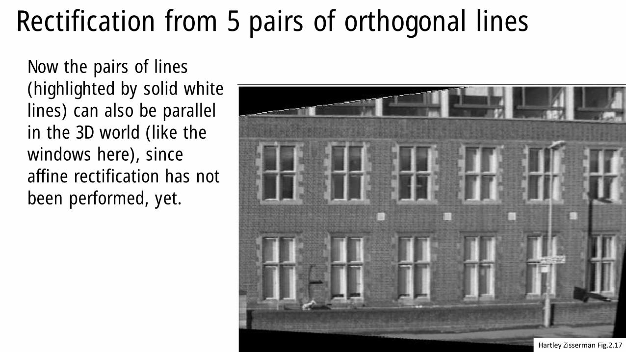
Rectification from 5 pairs of orthogonal lines
Now the pairs of lines
(highlighted by solid white
lines) can also be parallel
in the 3D world (like the
windows here), since
affine rectification has not
been performed, yet.
Hartley Zisserman Fig.2.17
Giacomo Boracchi
Camera Calibration and the 3D world
Giacomo Boracchi
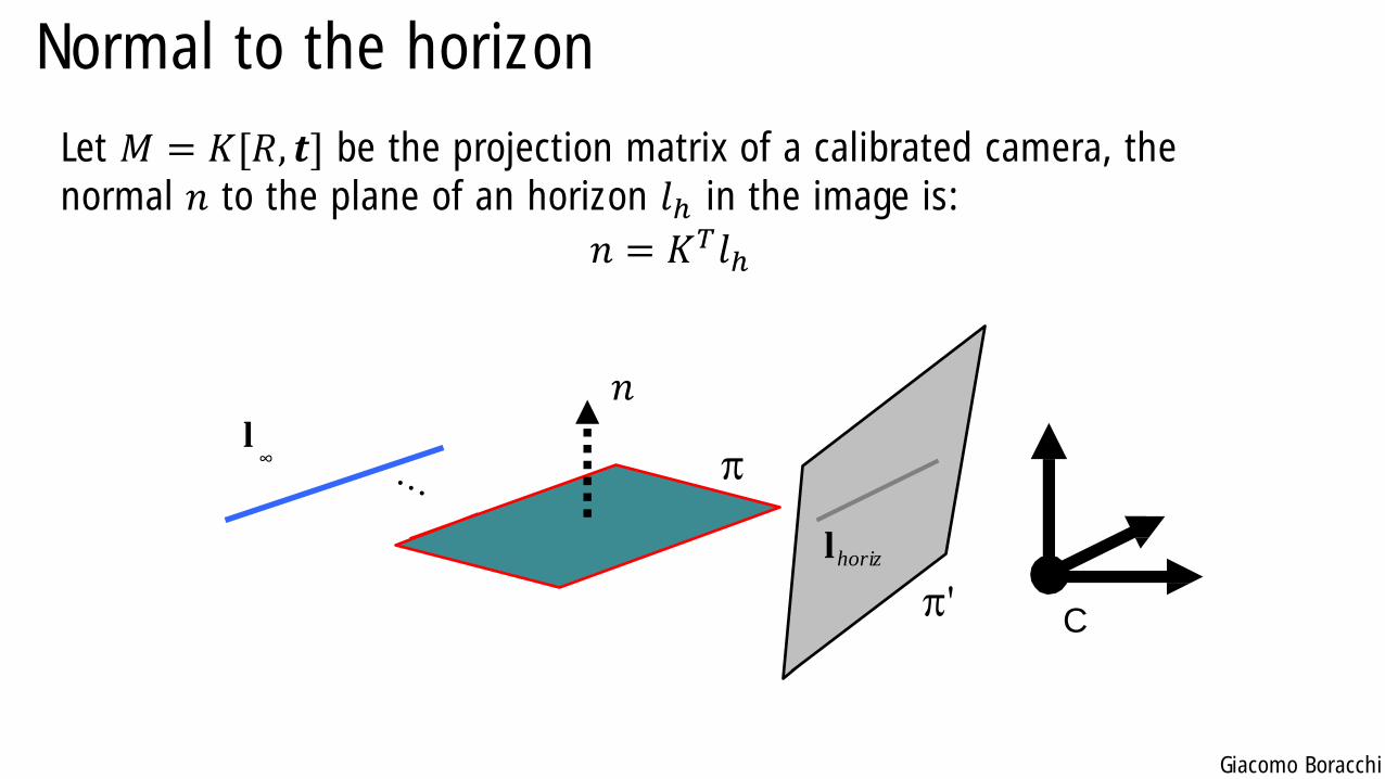
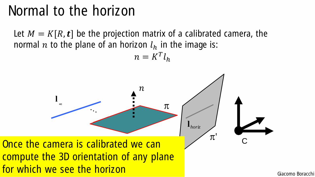
Normal to the horizon
Let 𝑀 = 𝐾[𝑅, 𝒕] be the projection matrix of a calibrated camera, the
normal 𝑛 to the plane of an horizon 𝑙ℎ in the image is:
𝑛 = 𝐾𝑇𝑙ℎ
C
𝑛
lhoriz
πl∞
π'
Giacomo Boracchi
Normal to the horizon
Let 𝑀 = 𝐾[𝑅, 𝒕] be the projection matrix of a calibrated camera, the
normal 𝑛 to the plane of an horizon 𝑙ℎ in the image is:
𝑛 = 𝐾𝑇𝑙ℎ
C
𝑛
lhoriz
πl∞
π'Once the camera is calibrated we can
compute the 3D orientation of any plane
for which we see the horizon
Giacomo Boracchi
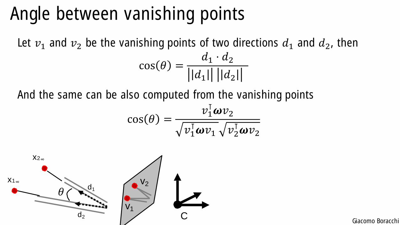
Angle between vanishing points
Let 𝑣1 and 𝑣2 be the vanishing points of two directions 𝑑1 and 𝑑2, then
cos 𝜃 =𝑑1 ⋅ 𝑑2
𝑑1 𝑑2
And the same can be also computed from the vanishing points
cos 𝜃 =𝑣1⊺𝝎𝑣2
𝑣1⊺𝝎𝑣1 𝑣2
⊺𝝎𝑣2
C
d1
v2
v1d2
𝜃x1∞
x2∞
Giacomo Boracchi
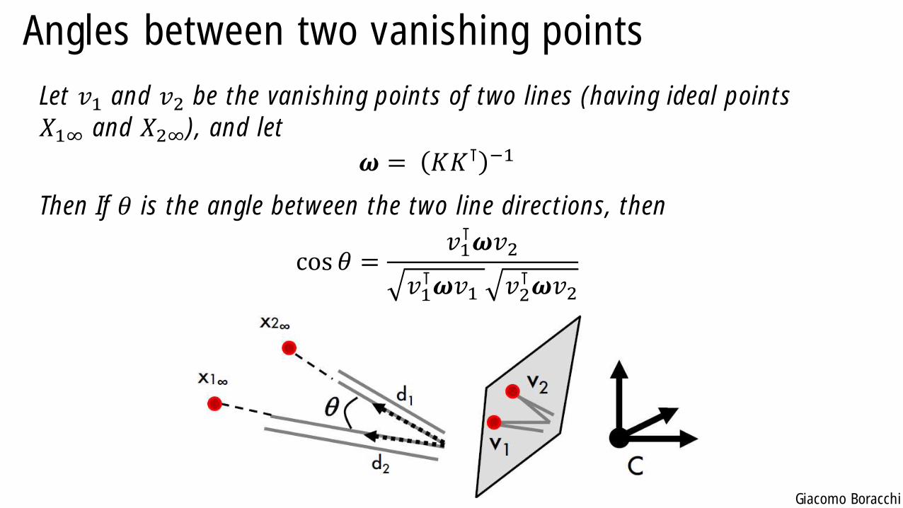
Angles between two vanishing points
Let 𝑣1 and 𝑣2 be the vanishing points of two lines (having ideal points
𝑋1∞ and 𝑋2∞), and let
𝝎 = 𝐾𝐾⊺ −1
Then If 𝜃 is the angle between the two line directions, then
cos 𝜃 =𝑣1⊺𝝎𝑣2
𝑣1⊺𝝎𝑣1 𝑣2
⊺𝝎𝑣2
Giacomo Boracchi
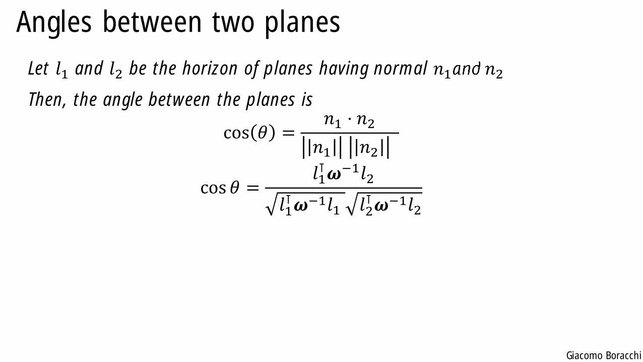
Angles between two planes
Let 𝑙1 and 𝑙2 be the horizon of planes having normal 𝑛1 𝑛2
Then, the angle between the planes is
cos 𝜃 =𝑛1 ⋅ 𝑛2
𝑛1 𝑛2
cos 𝜃 =𝑙1⊺𝝎−1𝑙2
𝑙1⊺𝝎−1𝑙1 𝑙2
⊺𝝎−1𝑙2
Giacomo Boracchi
Camera Calibration from Vanishing Points
Vanishing points are images of points at infinity, and provide orientation
information as fixed stars.
Ideal points are part of the scene and can be used as references. Their
position in the image (i.e. the vanishing points) depend only on the
camera rotation.
Giacomo Boracchi
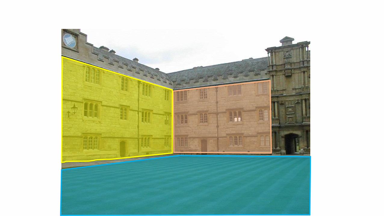
Calibration From 3D Orthogonal Vanishing Points
Note that any pair of vanishing point 𝑣1, 𝑣2 corresponding orthogonal
lines in the image yields a scalar equation in 𝝎
𝑣1⊺𝝎𝑣2
𝑣1⊺𝝎𝑣1 𝑣2
⊺𝝎𝑣2= 0
𝑣1⊺𝝎𝑣2 = 0
The matrix 𝝎 is symmetric (𝝎 = 𝐾𝐾⊺ −1), thus 5 unknonwns
𝝎 =
𝑤1 𝑤2 𝑤4
𝑤2 𝑤3 𝑤5
𝑤4 𝑤5 𝑤6
If the camera has zero skew 𝑤2 = 0
If pixels are squared 𝑤3 = 𝑤1
Giacomo Boracchi
Calibration From 3D Orthogonal Vanishing Points
The matrix 𝝎 is symmetric for a squared pixel and zeros-skew camera
𝝎 =𝑤1 0 𝑤4
0 𝑤1 𝑤5
𝑤4 𝑤5 𝑤6
This has 4 unknowns (up to a scalar factor) -> three pairs of orthogonal
lines can be used to compute 𝝎
Once 𝝎 has been computed, 𝐾 can be obtained by Cholesky factorization

Giacomo Boracchi
Giacomo Boracchi
Giacomo Boracchi
Giacomo Boracchi
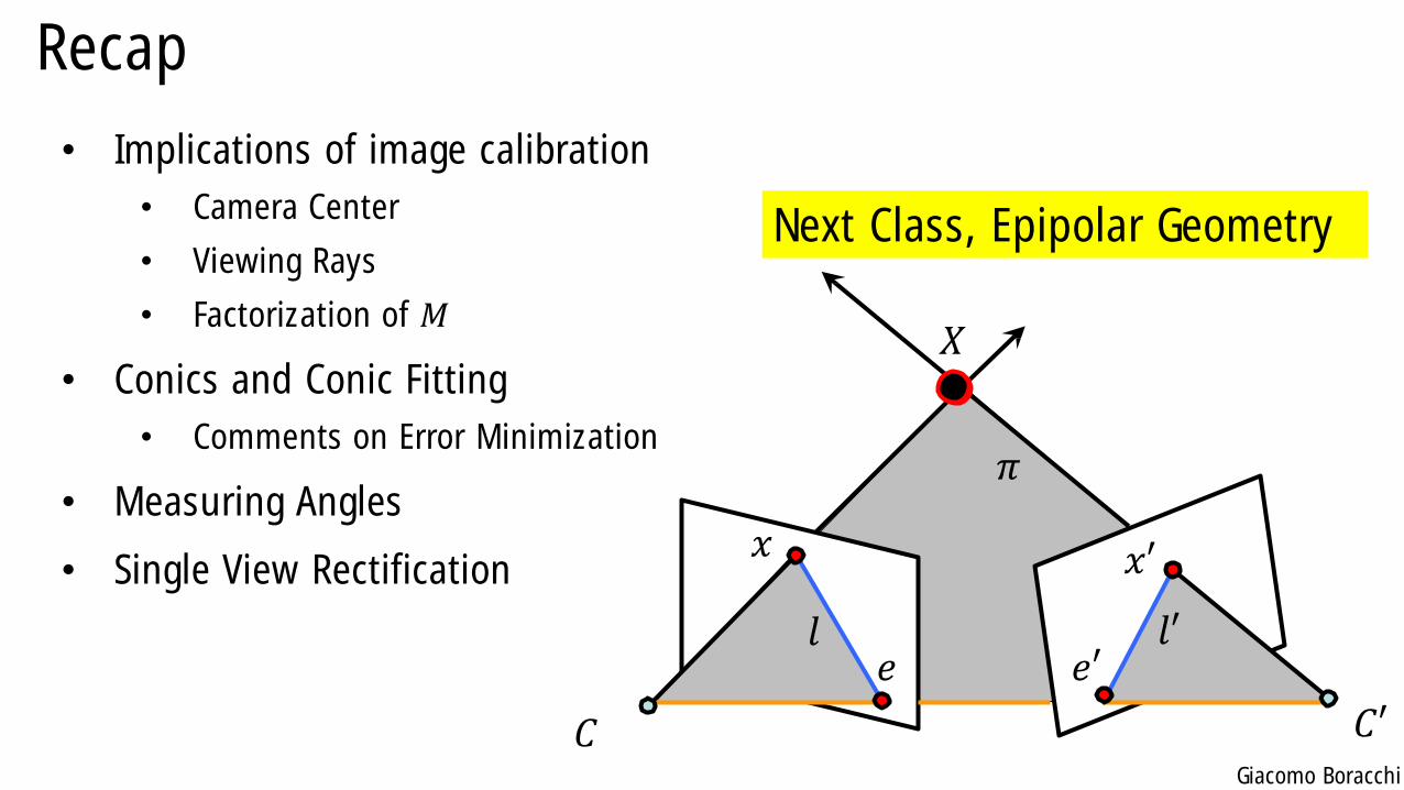
Recap
• Implications of image calibration
• Camera Center
• Viewing Rays
• Factorization of 𝑀
• Conics and Conic Fitting
• Comments on Error Minimization
• Measuring Angles
• Single View Rectification
Next Class, Epipolar Geometry
𝑥 𝑥′
𝑋
𝐶′𝐶
𝑒 𝑒′
𝜋
𝑙 𝑙′