hand and spreadsheet simulations - isyesman/courses/6644/module03-handsimulationslides... ·...

Hand and Spreadsheet Simulations

Christos Alexopoulos and Dave Goldsman

Georgia Institute of Technology, Atlanta, GA, USA

9/17/17

1 / 37

Outline

1 Stepping Through a Differential Equation

2 Monte Carlo Integration

3 Making Some π

4 Single-Server Queue

5 (s, S) Inventory System

6 Simulating Random Variables

7 Spreadsheet Simulation

2 / 37

Stepping Through a Differential Equation

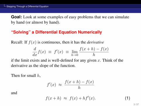
Goal: Look at some examples of easy problems that we can simulateby hand (or almost by hand).

“Solving” a Differential Equation Numerically

Recall: If f(x) is continuous, then it has the derivative

d

dxf(x) ≡ f ′(x) ≡ lim

h→0

f(x+ h)− f(x)

h

if the limit exists and is well-defined for any given x. Think of thederivative as the slope of the function.

Then for small h,

f ′(x) ≈ f(x+ h)− f(x)

hand

f(x+ h) ≈ f(x) + hf ′(x). (1)3 / 37


Example: Suppose you have a differential equation of a populationgrowth model, f ′(x) = 2f(x) with f(0) = 10. Let’s “solve” thisusing a fixed-increment time approach with h = 0.01. (This is knownas Euler’s method.) By (1), we have

f(x+ h) ≈ f(x) + hf ′(x) = f(x) + 2hf(x) = (1 + 2h)f(x).

Similarly,

f(x+2h) = f((x+h)+h) ≈ (1+2h)f(x+h) ≈ (1+2h)2f(x).

Continuing,

f(x+ ih) ≈ (1 + 2h)if(x) i = 0, 1, 2, . . . ,

though the approximation may deteriorate as i gets large.

4 / 37


Plugging in f(0) = 10 and h = 0.01, we have

f(0.01i) ≈ 10(1.02)i, i = 0, 1, 2, . . . . (2)

Now, I happen to know that the true solution to the differentialequation is f(x) = 10e2x. So the approximation (2) makes sensesince for small y,

ey =

∞∑`=0

y`

`!≈ 1 + y ≈ (1 + y)i for small i.

In any case, let’s see how well the approximation does. . . .

x = ih = 0.01i 0 0.01 0.02 0.03 0.04 · · · 0.10

approx f(x) ≈ 10(1.02)i 10 10.20 10.40 10.61 10.82 · · · 12.19

true f(x) = 10e2x 10 10.20 10.41 10.62 10.83 · · · 12.21

Not bad at all (at least for small i)! 25 / 37

Monte Carlo Integration

Outline



3 Making Some π





6 / 37



The previous differential equation example didn’t involve anyrandomness. That will change with the current Monte Carloapplication. Let’s integrate

I =

∫ b

ag(x) dx = (b− a)

∫ 1

0g(a+ (b− a)u) du,

where we get the last equality by substituting u = (x− a)/(b− a).

Of course, we can often do this by analytical methods that we learnedback in calculus class, or by numerical methods like the trapezoid ruleor something like Gauss-Laguerre integration. But if these methodsaren’t possible, you can always use MC integration. . . .

7 / 37


Suppose U1, U2, . . . are iid Unif(0,1), and define

Ii ≡ (b− a)g(a+ (b− a)Ui) for i = 1, 2, . . . , n.

We can use the sample average as an estimator for I:

In ≡1

n

n∑i=1

Ii =b− an

n∑i=1

g(a+ (b− a)Ui).

Why is this okey dokey? Let’s appeal to our old friend, the Law ofLarge Numbers: If an estimator is asymptotically unbiased and itsvariance goes to zero, then things are good.

8 / 37


First, by the Law of the Unconscious Statistician, notice that

E[In] = (b− a)E[g(a+ (b− a)Ui)]

= (b− a)

∫Rg(a+ (b− a)u)f(u) du

(where f(u) is the Unif(0,1) pdf)

= (b− a)

∫ 1

0g(a+ (b− a)u) du = I.

So In is unbiased for I .

Since it can also be shown that Var(In) = O(1/n), the LLN impliesIn → I as n→∞.

9 / 37


10 / 37


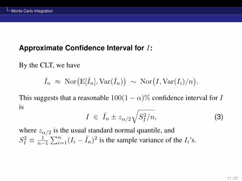
Approximate Confidence Interval for I:

By the CLT, we have

In ≈ Nor(E[In],Var(In)

)∼ Nor

(I,Var(Ii)/n

).

This suggests that a reasonable 100(1− α)% confidence interval for Iis

I ∈ In ± zα/2√S2I /n, (3)

where zα/2 is the usual standard normal quantile, andS2I ≡

1n−1

∑ni=1(Ii − In)2 is the sample variance of the Ii’s.

11 / 37


Example: Suppose I =∫ 10 sin(πx) dx (and pretend we don’t know

the actual answer, 2/π.= 0.6366).

Let’s take n = 4 Unif(0,1) observations:

U1 = 0.79 U2 = 0.11 U3 = 0.68 U4 = 0.31

Since

Ii = (b− a)g(a+ (b− a)Ui) = g(Ui) = sin(πUi),

we obtain

In =1

4

4∑i=1

Ii =1

4

4∑i=1

sin(πUi) = 0.656,

which is close to 2/π! (Actually, we got lucky.)

12 / 37


Moreover, the approximate 95% confidence interval for I from (3) is

I ∈ 0.656± 1.96√

0.0557/4 = [0.596, 0.716].

And we’ll usually do better as n gets big — though sometimes theconvergence is choppy due to good or bad luck. 2

13 / 37

Making Some π

Outline



3 Making Some π





14 / 37

Making Some π

Making Some π

Consider a unit square (with area one). Inscribe in the square a circlewith radius 1/2 (with area π/4). Suppose we toss darts randomly atthe square. The probability that a particular dart will land in theinscribed circle is obviously π/4 (the ratio of the two areas). We canuse this fact to estimate π.

Toss n such darts at the square and calculate the proportion pn thatland in the circle. Then an estimate for π is πn = 4pn, whichconverges to π as n becomes large by the LLN.

For instance, suppose that we throw n = 500 darts at the square and397 of them land in the circle. Then pn = 0.794, and our estimate forπ is πn = 3.176 — not so bad.

15 / 37

Making Some π

16 / 37

Making Some π

How would we actually conduct such an experiment?

To simulate a dart toss, suppose U1 and U2 are iid Unif(0,1). Then(U1, U2) represents the random position of the dart on the unit square.The dart lands in the circle if(

U1 −1

2

)2

+

(U2 −

1

2

)2

≤ 1

4.

Generate n such pairs of uniforms and count up how many of themfall in the circle. Then plug into πn. 2

17 / 37

Single-Server Queue

Outline



3 Making Some π





18 / 37

Single-Server Queue

Single-Server QueueCustomers arrive at a single-server Q with iid interarrival times and iidservice times. Customers must wait in a FIFO Q if the server is busy.

We will estimate the expected customer waiting time, the expectednumber of people in the system, and the server utilization (proportionof busy time). First, some notation.

Interarrival time between customers i− 1 and i is IiCustomer i’s arrival time is Ai =

∑ij=1 Ij

Customer i starts service at time Ti = max(Ai, Di−1)

Customer i’s waiting time is WQi = Ti −Ai

Customer i’s time in the system is Wi = Di −AiCustomer i’s service time is SiCustomer i’s departure time is Di = Ti + Si

19 / 37

Single-Server Queue

Example: Suppose we have the following sequence of events. . .

i Ii Ai Ti WQi Si Di

1 3 3 3 0 7 10

2 1 4 10 6 6 16

3 2 6 16 10 4 20

4 4 10 20 10 6 26

5 5 15 26 11 1 27

6 5 20 27 7 2 29

The average waiting time for the six customers is obviously∑6i=1W

Qi /6 = 7.33.

How do we get the average number of people in the system (in line +in service)?

20 / 37

Single-Server Queue

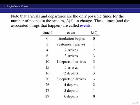
Note that arrivals and departures are the only possible times for thenumber of people in the system, L(t), to change. These times (and theassociated things that happen) are called events.

time t event L(t)

0 simulation begins 03 customer 1 arrives 14 2 arrives 26 3 arrives 3

10 1 departs; 4 arrives 315 5 arrives 416 2 departs 320 3 departs; 6 arrives 326 4 departs 227 5 departs 129 6 departs 0

21 / 37

Single-Server Queue

L(t)

5 Queue customer 3 4 4 5 6 2 2 3 3 4 5 6 in 1 1 1 2 2 3 4 5 6 service t

3 4 6 10 15 16 20 26 27 29

The average number in the system is L = 129

∫ 290 L(t) dt = 70

29 . 2

22 / 37

Single-Server Queue

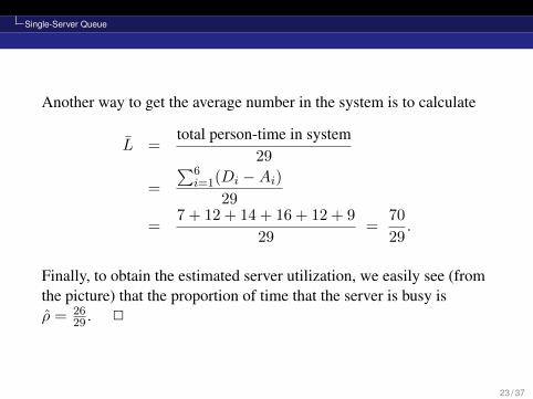
Another way to get the average number in the system is to calculate

L =total person-time in system

29

=

∑6i=1(Di −Ai)

29

=7 + 12 + 14 + 16 + 12 + 9

29=

70

29.

Finally, to obtain the estimated server utilization, we easily see (fromthe picture) that the proportion of time that the server is busy isρ = 26

29 . 2

23 / 37

Single-Server Queue

Example: Same events, but last-in-first-out (LIFO) services. . .

i Ii Ai Ti WQi Si Di

1 3 3 3 0 7 10

2 1 4 23 19 6 29

3 2 6 17 11 4 21

4 4 10 10 0 6 16

5 5 15 16 1 1 17

6 5 20 21 1 2 23

The average waiting time for the six customers is 5.33, and theaverage number of people in the system turns out to be 58

29 = 2, whichin this case turn out to be better than FIFO.

24 / 37

(s, S) Inventory System

Outline



3 Making Some π





25 / 37


(s, S) Inventory SystemA store sells a product at $d/unit. Our inventory policy is to have atleast s units in stock at the start of each day. If the stock slips to lessthan s by the end of the day, we place an order with our supplier topush the stock back up to S by the beginning of the next day.

Let Ii denote the inventory at the end of day i, and let Zi denote theorder that we place at the end of day i. Clearly,

Zi =

{S − Ii if Ii < s

0 otherwise.

If an order is placed to the supplier at the end of day i, it costs thestore K + cZi. It costs $h/unit for the store to hold unsold inventoryovernight, and a penalty cost of $p/unit if demand can’t be met. Nobacklogs are allowed. Demand on day i is Di.

26 / 37


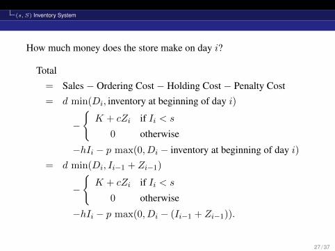
How much money does the store make on day i?

Total

= Sales − Ordering Cost − Holding Cost − Penalty Cost

= d min(Di, inventory at beginning of day i)

−

{K + cZi if Ii < s

0 otherwise

−hIi − p max(0, Di − inventory at beginning of day i)

= d min(Di, Ii−1 + Zi−1)

−

{K + cZi if Ii < s

0 otherwise

−hIi − p max(0, Di − (Ii−1 + Zi−1)).

27 / 37


Example: Suppose

d = 10, s = 3, S = 10, K = 2, c = 4, h = 1, p = 2.

Consider the following sequence of demands:

D1 = 5, D2 = 2, D3 = 8, D4 = 6, D5 = 2, D6 = 1.

Suppose that we start out with an initial stock of I0 + Z0 = 10.

Day begin sales order hold penalty TOTALi stock Di Ii Zi rev cost cost cost rev

1 10 5 5 0 50 0 −5 0 452 5 2 3 0 20 0 −3 0 173 3 8 0 10 30 −42 0 −10 −224 10 6 4 0 60 0 −4 0 565 4 2 2 8 20 −34 −2 0 −166 10 1 9 0 10 0 −9 0 1

28 / 37

Simulating Random Variables

Outline



3 Making Some π





29 / 37



Example (Discrete Uniform): Consider a D.U. on {1, 2, . . . , n},i.e., X = i with probability 1/n for i = 1, 2, . . . , n. (Think of this asan n-sided dice toss for you Dungeons and Dragons fans.)

If U ∼ Unif(0, 1), we can obtain a D.U. random variate simply bysetting X = dnUe, where d·e is the “ceiling” (or “round up”)function.

For example, if n = 10 and we sample a Unif(0,1) random variableU = 0.73, then X = d7.3e = 8. 2

30 / 37


Example (Another Discrete Random Variable):

P (X = x) =

0.25 if x = −2

0.10 if x = 3

0.65 if x = 4.2

0 otherwise

Can’t use a die toss to simulate this random variable. Instead, usewhat’s called the inverse transform method.

x P (X = x) P (X ≤ x) Unif(0,1)’s

−2 0.25 0.25 [0.00, 0.25]3 0.10 0.35 (0.25, 0.35]

4.2 0.65 1.00 (0.35, 1.00)

Sample U ∼ Unif(0, 1). Choose the corresponding x-value, i.e.,X = F−1(U). For example, U = 0.46 means that X = 4.2. 2

31 / 37


Now we’ll use the inverse transform method to generate a continuousrandom variable. Recall. . .

Theorem: If X is a continuous random variable with cdf F (x), thenthe random variable F (X) ∼ Unif(0, 1).

This suggests a way to generate realizations of the RV X . Simply setF (X) = U ∼ Unif(0, 1) and solve for X = F−1(U).

Old Example: Suppose X ∼ Exp(λ). Then F (x) = 1− e−λx forx > 0. Set F (X) = 1− e−λX = U . Solve for X ,

X =−1

λ`n(1− U) ∼ Exp(λ). 2

32 / 37


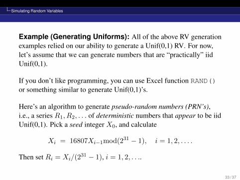
Example (Generating Uniforms): All of the above RV generationexamples relied on our ability to generate a Unif(0,1) RV. For now,let’s assume that we can generate numbers that are “practically” iidUnif(0,1).

If you don’t like programming, you can use Excel function RAND()or something similar to generate Unif(0,1)’s.

Here’s an algorithm to generate pseudo-random numbers (PRN’s),i.e., a series R1, R2, . . . of deterministic numbers that appear to be iidUnif(0,1). Pick a seed integer X0, and calculate

Xi = 16807Xi−1mod(231 − 1), i = 1, 2, . . . .

Then set Ri = Xi/(231 − 1), i = 1, 2, . . ..

33 / 37


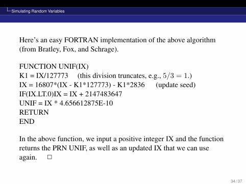
Here’s an easy FORTRAN implementation of the above algorithm(from Bratley, Fox, and Schrage).

FUNCTION UNIF(IX)K1 = IX/127773 (this division truncates, e.g., 5/3 = 1.)IX = 16807*(IX - K1*127773) - K1*2836 (update seed)IF(IX.LT.0)IX = IX + 2147483647UNIF = IX * 4.656612875E-10RETURNEND

In the above function, we input a positive integer IX and the functionreturns the PRN UNIF, as well as an updated IX that we can useagain. 2

34 / 37

Spreadsheet Simulation

Outline



3 Making Some π





35 / 37


Spreadsheet SimulationLet’s simulate a fake stock portfolio consisting of 6 stocks fromdifferent sectors, as laid out in my Excel file Spreadsheet StockPortfolio. We start out with $5000 worth of each stock, and eachincreases or decreases in value each year according to

Previous Value * max[

0, Nor(µi, σ

2i

)* Nor

(1, (0.2)2

) ],

where the first normal term denotes the natural stock fluctuation forstock i, and the second normal denotes natural market conditions (thataffect all stocks).

To generate a normal in Excel, you can use

NORM.INV(RAND(),µ,σ ) ,

where RAND() is Unif(0,1), so that NORM.INV uses the inversetransform method.

36 / 37


37 / 37

hand and spreadsheet simulations - isyesman/courses/6644/module03-handsimulationslides... ·...

Documents