hydrodynamics continuity equation - aia · hydrodynamics continuity equation ... diffusor...
TRANSCRIPT
Hydrodynamics
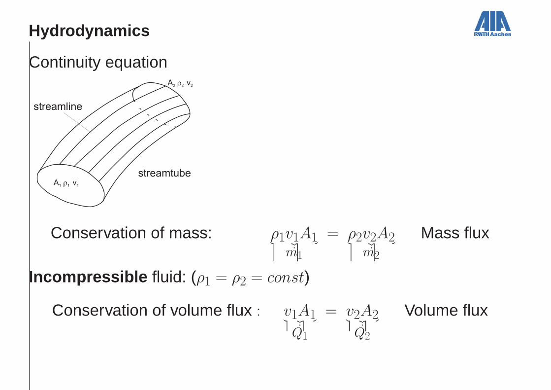
Continuity equation
streamline
streamtubeA
1r
1v
1
A2
r2
v2
Conservation of mass: ρ1v1A1︸ ︷︷ ︸
m1
= ρ2v2A2︸ ︷︷ ︸
m2
Mass flux
Incompressible fluid: (ρ1 = ρ2 = const)
Conservation of volume flux : v1A1︸ ︷︷ ︸
Q1
= v2A2︸ ︷︷ ︸
Q2
Volume flux
Hydrodynamics
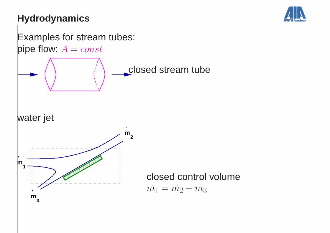
Examples for stream tubes:pipe flow: A = const
closed stream tube
water jet
m
������������������������������������������������������������������������������������������������������������������������
������������������������������������������������������������������������������������������������������������������������
3
m1
m2
closed control volumem1 = m2 + m3
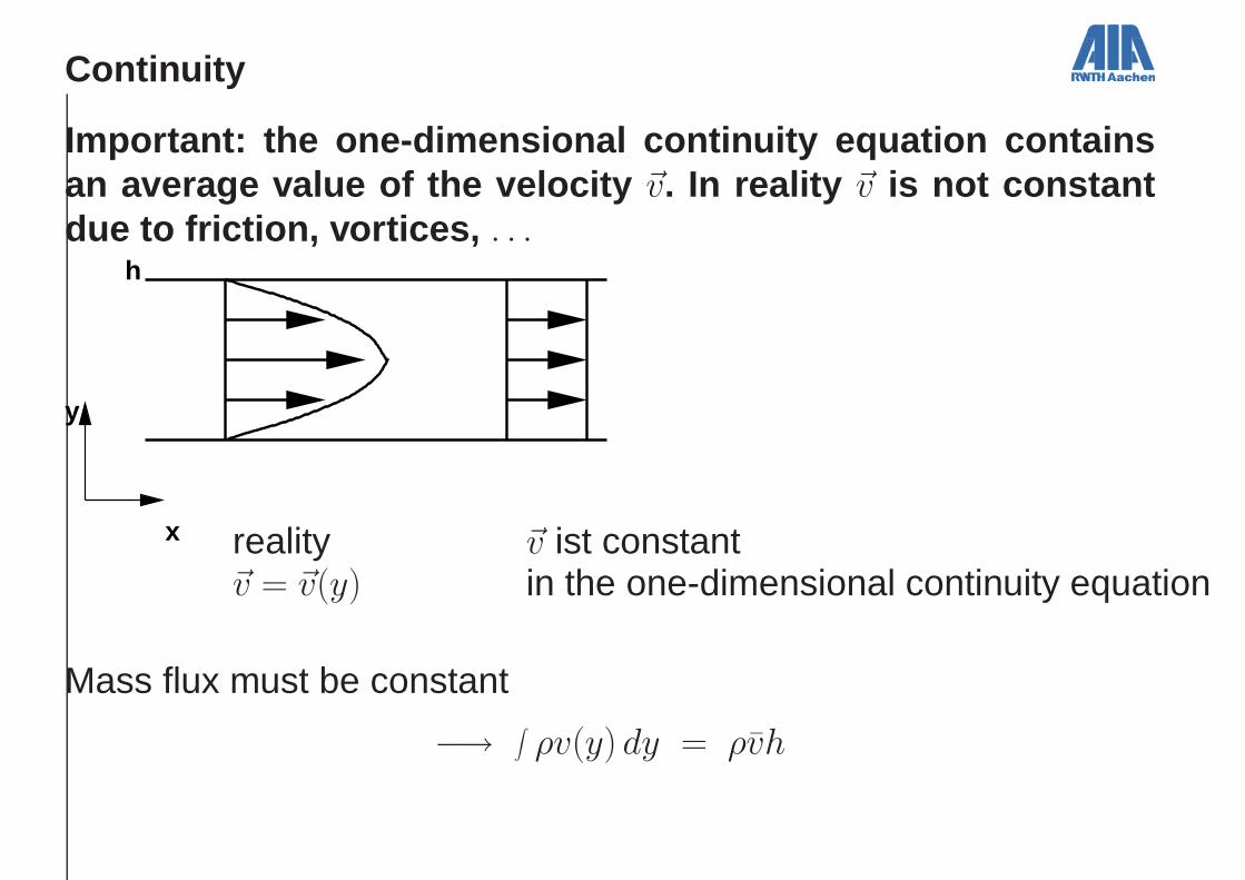
Continuity
Important: the one-dimensional continuity equation conta insan average value of the velocity ~v. In reality ~v is not constantdue to friction, vortices, . . .
x
y
h
reality~v = ~v(y)
~v ist constantin the one-dimensional continuity equation
Mass flux must be constant
−→∫
ρv(y) dy = ρvh
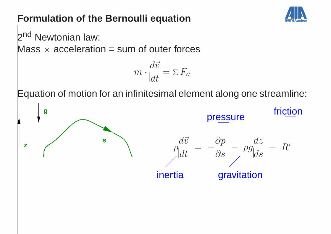
Formulation of the Bernoulli equation
2nd Newtonian law:Mass × acceleration = sum of outer forces
m ·d~v
dt=
∑
Fa
Equation of motion for an infinitesimal element along one streamline:
sz
g
ρd~v
dt= −
∂p
∂s− ρg
dz
ds− R‘
��
�
inertia
pressure
��
�
gravitation
friction
Formulation of the Bernoulli equation
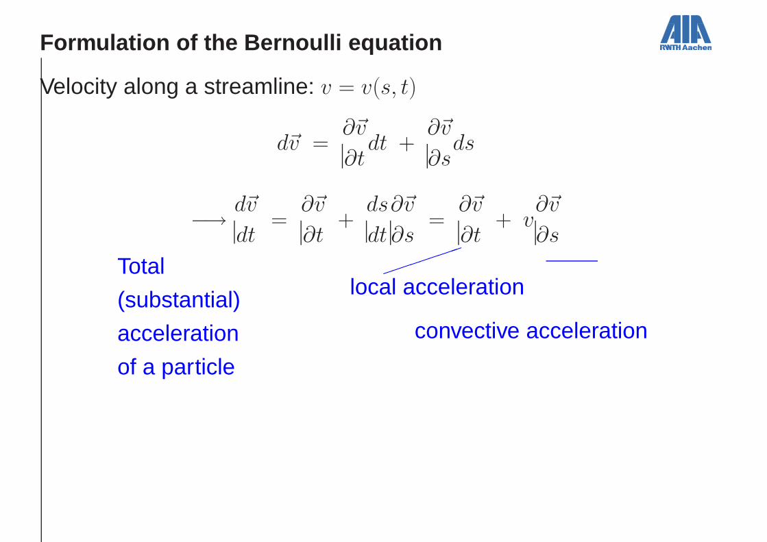
Velocity along a streamline: v = v(s, t)
d~v =∂~v
∂tdt +
∂~v
∂sds
−→d~v
dt=
∂~v
∂t+
ds
dt
∂~v
∂s=
∂~v
∂t+ v
∂~v
∂s
Total
(substantial)
acceleration
of a particle
���������
local acceleration
convective acceleration
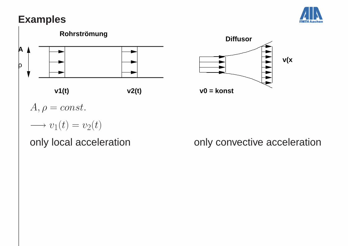
Examples
v(x)
A
v1(t) v2(t)
ρ
DiffusorRohrströmung
v0 = konst
A, ρ = const.
−→ v1(t) = v2(t)
only local acceleration only convective acceleration
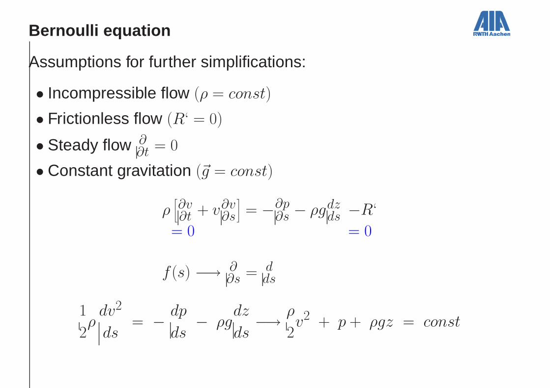
Bernoulli equation
Assumptions for further simplifications:
• Incompressible flow (ρ = const)
• Frictionless flow (R‘ = 0)
• Steady flow ∂∂t = 0
• Constant gravitation (~g = const)
ρ
∂v∂t + v∂v
∂s
= −∂p∂s − ρgdz
ds −R‘
= 0 = 0
f (s) −→ ∂∂s = d
ds
1
2ρ
dv2
ds= −
dp
ds− ρg
dz
ds−→
ρ
2v2 + p + ρgz = const
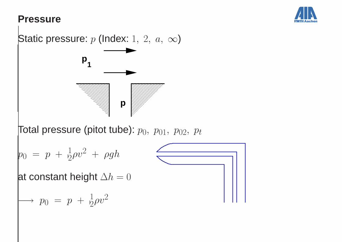
Pressure
Static pressure: p (Index: 1, 2, a, ∞)
�������������������������������������������������������������������������������������������
�������������������������������������������������������������������������������������������
������������������������������������������������������������������������������
������������������������������������������������������������������������������
��������������
p
p1
Total pressure (pitot tube): p0, p01, p02, pt
p0 = p + 12ρv2 + ρgh
at constant height ∆h = 0
−→ p0 = p + 12ρv2

Pressures
Potential pressure: ppot = ρgh
���������������������������������������������������������
���������������������������������������������������������
h
Dynamic pressure: pdyn = 12ρv2
kinetic energy is converted, when the flow is decelerated to ~v = 0
Example 7
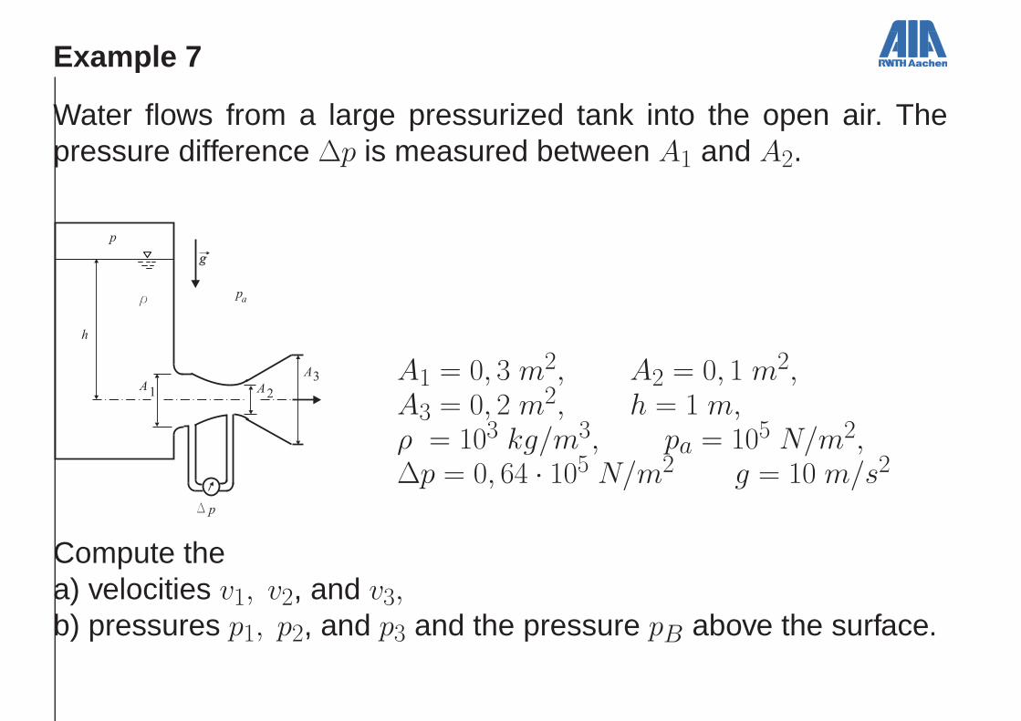
Water flows from a large pressurized tank into the open air. Thepressure difference ∆p is measured between A1 and A2.
A1 = 0, 3 m2, A2 = 0, 1 m2,A3 = 0, 2 m2, h = 1 m,ρ = 103 kg/m3, pa = 105 N/m2,∆p = 0, 64 · 105 N/m2 g = 10 m/s2
Compute thea) velocities v1, v2, and v3,b) pressures p1, p2, and p3 and the pressure pB above the surface.
Example 7
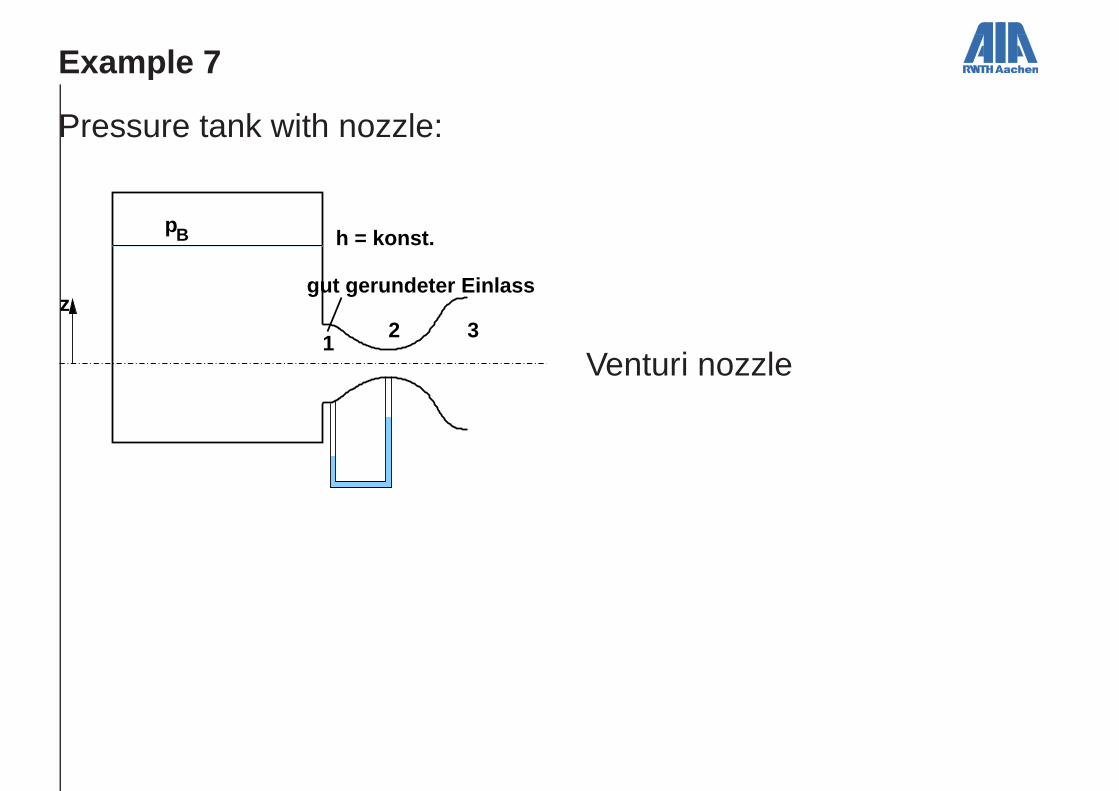
Pressure tank with nozzle:
z
12 3
pB h = konst.
gut gerundeter Einlass
Venturi nozzle
Example 7
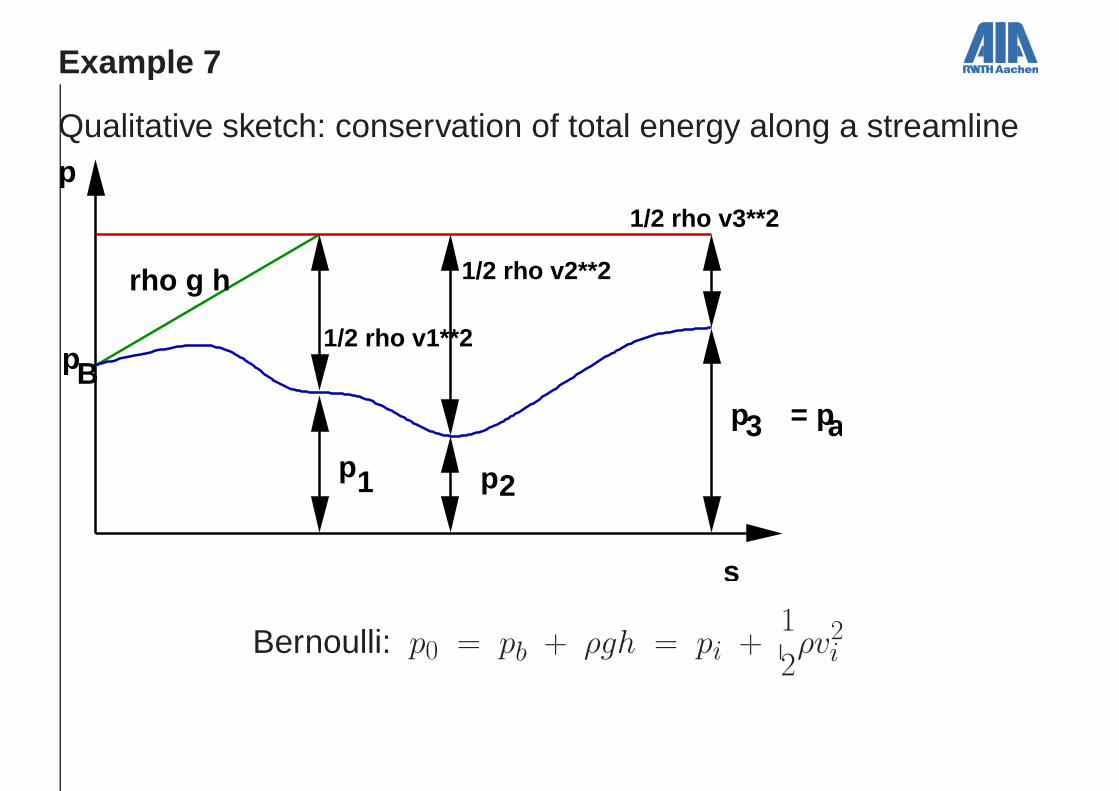
Qualitative sketch: conservation of total energy along a streamlinep
p
s
pp
B
1 2
p3 = pa
rho g h
1/2 rho v1**2
1/2 rho v2**2
1/2 rho v3**2
Bernoulli: p0 = pb + ρgh = pi +1
2ρv2
i

Example 7
Continuity (mass balance): → = m = ρQ = const.
ρ = const → v1A1 = v2A2 = v3A3 → A ↓ → v ↑ → p ↓
a) Measured ∆p = p1 − p2 Bernoulli: p1 + ρ2v
21 = p2 + ρ
2v22
→ ∆p = p1 − p2 =ρ
2(v2
2 − v21) > 0
v1 = v2A2
A1→ ∆p =
ρ
2
1 −A2
2
A21
v22 → v2 =
√√√√√√√√√√√√
2
ρ
∆p
1 −
A2A1
2
= 12m
s
v1 = v2A2
A1= 4
m
sv3 = v2
A2
A3= 6
m
s
Example 7
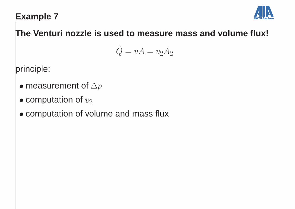
The Venturi nozzle is used to measure mass and volume flux!
Q = vA = v2A2
principle:
• measurement of ∆p
• computation of v2
• computation of volume and mass flux
Example 7
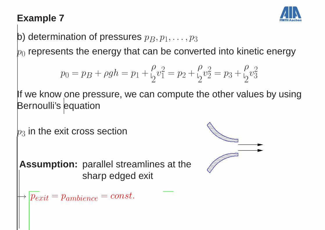
b) determination of pressures pB, p1, . . . , p3
p0 represents the energy that can be converted into kinetic energy
p0 = pB + ρgh = p1 +ρ
2v21 = p2 +
ρ
2v22 = p3 +
ρ
2v23
If we know one pressure, we can compute the other values by usingBernoulli’s equation
p3 in the exit cross section
Assumption: parallel streamlines at thesharp edged exit
������������������������������������������������������������������������������������������������������������������������������������������������������������������������������������
������������������������������������������������������������������������������������������������������������������������������������������������������������������������������������
������������������������������������������������������������������������������������������������������������������������������������������������������������������������������������
������������������������������������������������������������������������������������������������������������������������������������������������������������������������������������
→ pexit = pambience = const.
Example 7
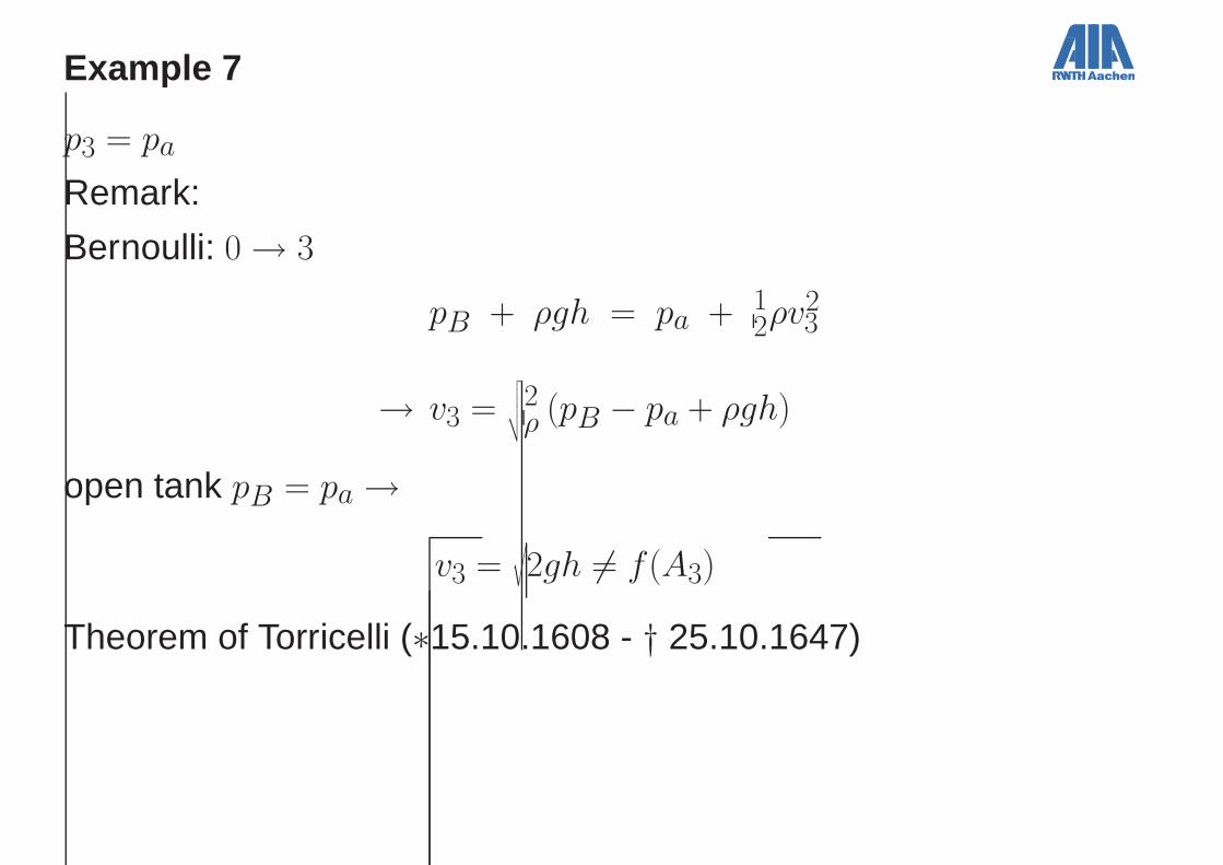
p3 = pa
Remark:
Bernoulli: 0 → 3
pB + ρgh = pa + 12ρv2
3
→ v3 =√√√√√2ρ (pB − pa + ρgh)
open tank pB = pa →
v3 =√
2gh 6= f (A3)
Theorem of Torricelli (∗15.10.1608 - † 25.10.1647)

Example 8
Two large basins located one upon the other are connected with aduct.
A = 1 m2 Ad = 0.1 m2 h = 5 m H = 80 m
pa = 105 N/m2 ρ = 103 kg/m3 g = 10 m/s2
a) Determine the volume rate.b) Outline the distribution of the static pressure in the duct.c) Which exit cross section is necessary to produce bubbles, if thevapour pressure equals pD = 0.025 · 105 N/m2?
Example 8
gh
HA
Ad
par
5
4
32
1
v
s
z
0
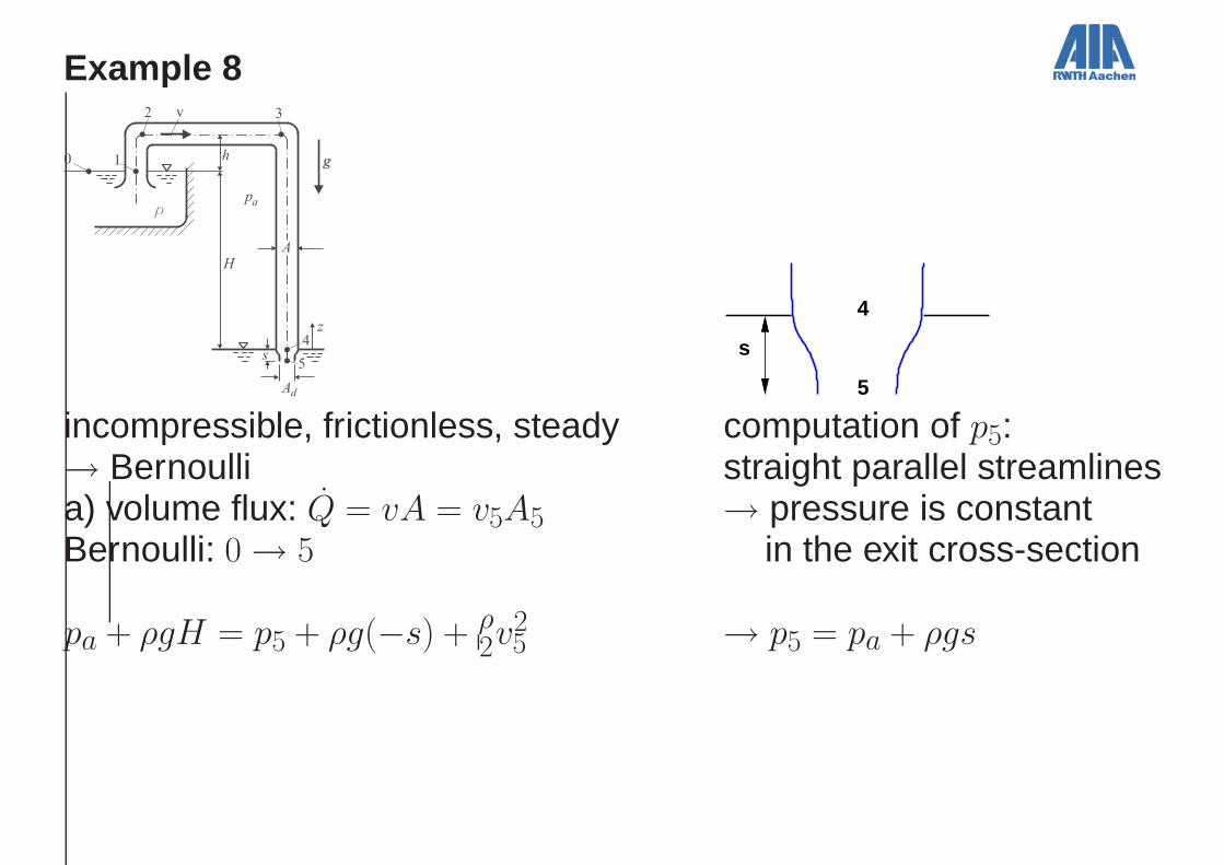
incompressible, frictionless, steady→ Bernoullia) volume flux: Q = vA = v5A5Bernoulli: 0 → 5
pa + ρgH = p5 + ρg(−s) + ρ2v
25
s
4
5
computation of p5:straight parallel streamlines→ pressure is constant
in the exit cross-section
→ p5 = pa + ρgs
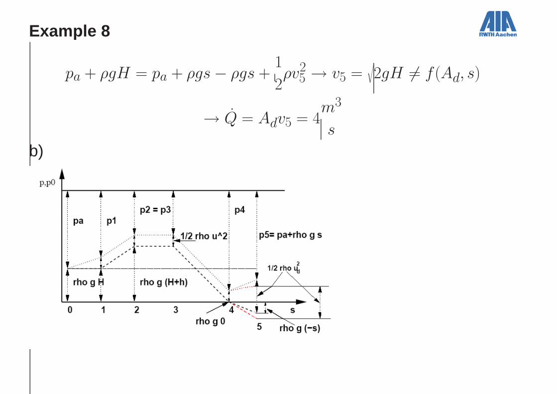
Example 8
pa + ρgH = pa + ρgs − ρgs +1
2ρv2
5 → v5 =√
2gH 6= f (Ad, s)
→ Q = Adv5 = 4m3
s
b)
Example 8
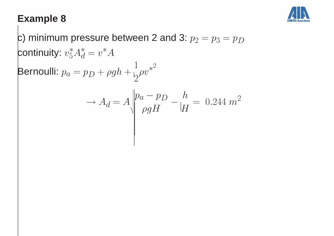
c) minimum pressure between 2 and 3: p2 = p3 = pD
continuity: v∗5A∗d = v∗A
Bernoulli: pa = pD + ρgh +1
2ρv∗
2
→ Ad = A
√√√√√√√√
pa − pD
ρgH−
h
H= 0.244 m2
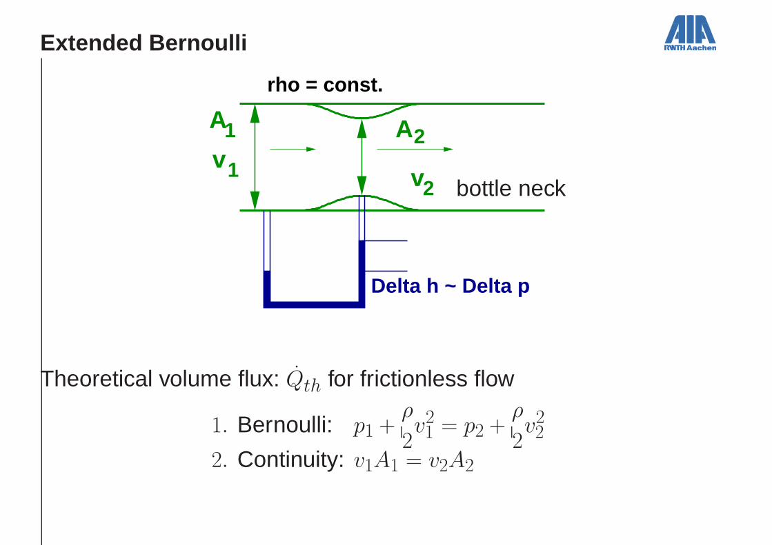
Extended Bernoulli
A Av1
2
rho = const.
Delta h ~ Delta p
2v
1
bottle neck
Theoretical volume flux: Qth for frictionless flow
1. Bernoulli: p1 +ρ
2v21 = p2 +
ρ
2v22
2. Continuity: v1A1 = v2A2
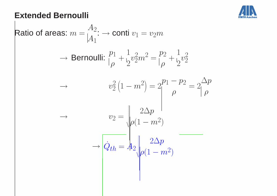
Extended Bernoulli
Ratio of areas: m =A2
A1: → conti v1 = v2m
→ Bernoulli:p1
ρ+
1
2v22m
2 =p2
ρ+
1
2v22
→ v22
1 − m2
= 2p1 − p2
ρ= 2
∆p
ρ
→ v2 =
√√√√√√√√√
2∆p
ρ(1 − m2)
→ Qth = A2
√√√√√√√√√
2∆p
ρ(1 − m2)

Extended Bernoulli
In reality losses from friction, vortices, bottle necks, . . . occur.→ the flow is no longer frictionless
The losses and the ratio of areas are put together in thedischarge coefficient α⋆
vortex, dissipation
Qreal = αA2
√√√√√√√√√
2∆p
ρ(1 − m2)
α⋆ = α
√√√√√√√√
1
1 − m2
α⋆ from experiments
Losses in pipe flows can be predicted similar.
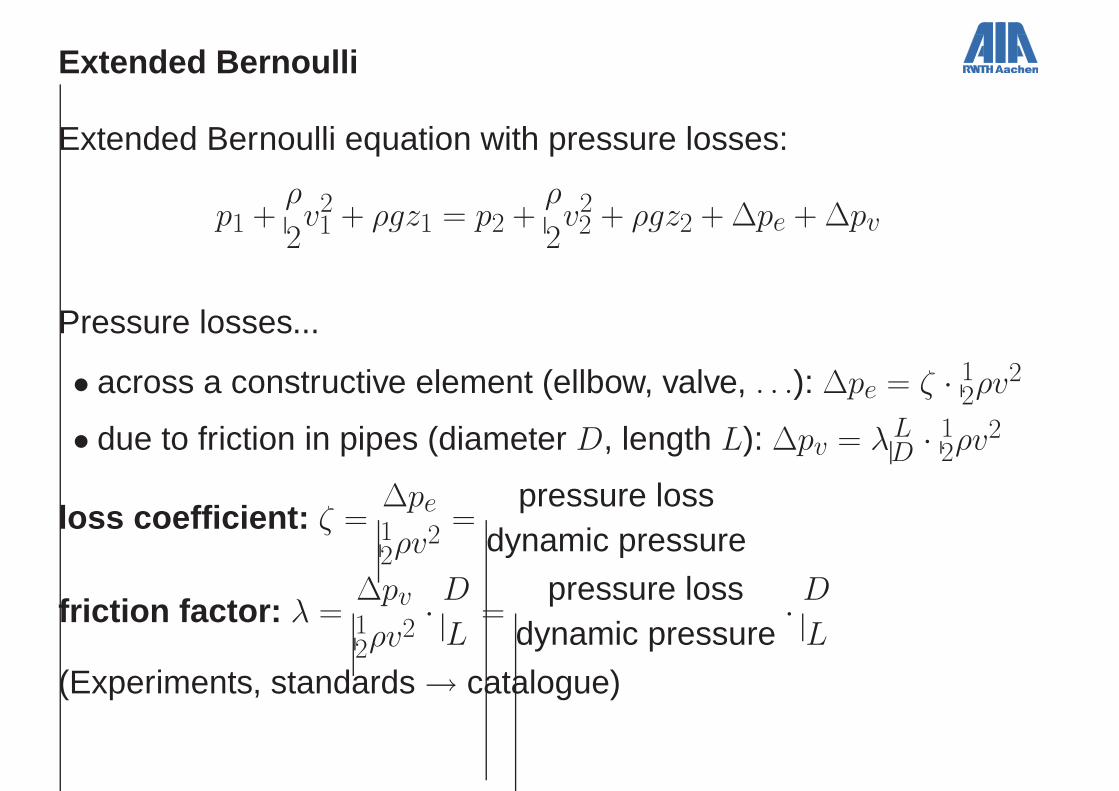
Extended Bernoulli
Extended Bernoulli equation with pressure losses:
p1 +ρ
2v21 + ρgz1 = p2 +
ρ
2v22 + ρgz2 + ∆pe + ∆pv
Pressure losses...
• across a constructive element (ellbow, valve, . . .): ∆pe = ζ · 12ρv2
• due to friction in pipes (diameter D, length L): ∆pv = λLD · 1
2ρv2
loss coefficient: ζ =∆pe12ρv2
=pressure loss
dynamic pressure
friction factor: λ =∆pv12ρv2
·D
L=
pressure lossdynamic pressure
·D
L
(Experiments, standards → catalogue)
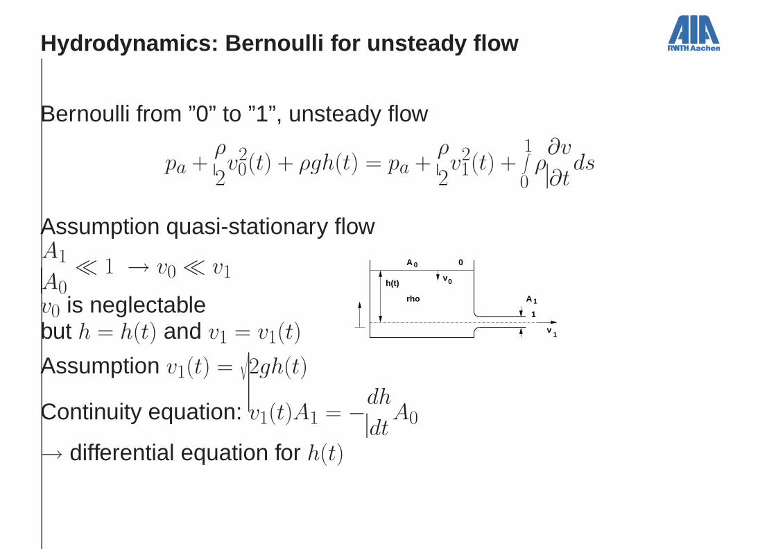
Hydrodynamics: Bernoulli for unsteady flow
Bernoulli from ”0” to ”1”, unsteady flow
pa +ρ
2v20(t) + ρgh(t) = pa +
ρ
2v21(t) +
1∫
0ρ∂v
∂tds
rho
h(t)v
A
A
v
0
1
0
1
1
0
Assumption quasi-stationary flowA1
A0≪ 1 → v0 ≪ v1
v0 is neglectablebut h = h(t) and v1 = v1(t)
Assumption v1(t) =√
2gh(t)
Continuity equation: v1(t)A1 = −dh
dtA0
→ differential equation for h(t)