Importance of Road

Freight Transport to the

Organization and Economy

Amal S. Kumarage

July 2014

Freight Transport

• FT is the process of conveying different types of goods

from one point to another using a variety

of transport modes.

• Hence FT is NOT site specific as other logistic activities.

• Transportation create the place and time value (utility)

• High Transport Costs can off set manufacturing gains

and reduce market size.

Po

Po

d

Pd = Po + rd

•Where Pd is the cost at distance d where Po is the cost at point of pick up

and r is the trucking rate per unit distance

•If production costs are similar and trucking costs are similar each producer and

each trucker will have the same volumes

•The market area is ˄ d2

Po

Po

1.1xd

Pd = Po + rd

•If one trucker is able to offer a 10% lower rate,

•Then the product is competitive at 1.1x d distance from the point of production

•The market area then increase to is ˄ (1.1xd)2

•This means that the market size has increase by 23%

•This shows that when transport cost reduces by 10% then market size increases by

21% and when transport cost reduces by 20% then market size will increase by 36%

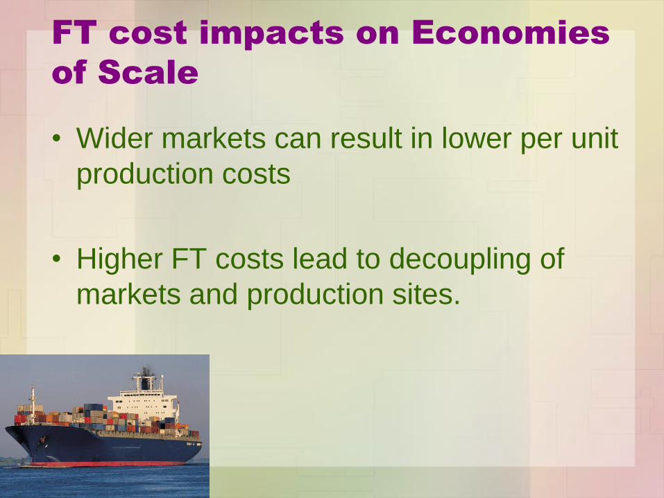
FT cost impacts on Economies

of Scale

• Wider markets can result in lower per unit

production costs

• Higher FT costs lead to decoupling of

markets and production sites.

Global Transport Costs as % of Logistics

Costs is Increasing

6

1980

GDP $2.88 trillion

Logistics Cost $451 billion

15.7% of GDP

Trans. Cost $214 billion

47.5 % of Logistics Cost

1999

GDP $9.26 trillion

Logistics Cost $921 billion

9.9% of GDP

Trans. Cost $554 billion

60.2 % of Logistics Cost

2013

GDP $74.5 trillion

Logistics Cost $ 7,012 billion

9.3% of GDP

Trans. Cost $3,500 billion

60 % of Logistics Cost

Source: IMF, World Economic Outlook

2013 (Sri Lanka)

GDP $70 million

Logistics Cost $ 9 million

13% of GDP

Trans. Cost $ 5 million

60 % of Logistics Cost

USA

Instances of Transport Cost

addition

9

Transport as % of

Logistics Costs

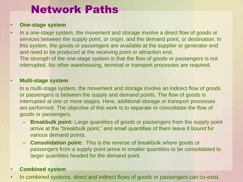
Network Paths

• One-stage system

• In a one-stage system, the movement and storage involve a direct flow of goods or

services between the supply point, or origin, and the demand point, or destination. In

this system, the goods or passengers are available at the supplier or generator end

and need to be produced at the receiving point or attraction end.

The strength of the one-stage system is that the flow of goods or passengers is not

interrupted. No other warehousing, terminal or transport processes are required.

• Multi-stage system

In a multi-stage system, the movement and storage involve an indirect flow of goods

or passengers is between the supply and demand points. The flow of goods is

interrupted at one or more stages. Here, additional storage or transport processes

are performed. The objective of this work is to separate or consolidate the flow of

goods or passengers.

– Breakbulk point: Large quantities of goods or passengers from the supply point

arrive at the “breakbulk point,” and small quantities of them leave it bound for

various demand points.

– Consolidation point: This is the reverse of breakbulk where goods or

passengers from a supply point arrive in smaller quantities to be consolidated to

larger quantities headed for the demand point.

• Combined system

• In combined systems, direct and indirect flows of goods or passengers can co-exist.

How do firms react to improvements

in freight Transportation

Firms reduce stocking points, increase JIT processes and increasing shipping distance.

Firms react to reduced late-shipping-delays, values highly by shippers by investing more in logistics.

Inter-industry trading partners are affected

Improvements in Network

Connectivity and Density

Industry Investment in

Advanced Logistics

Industrial Reorganization and Enhanced

Productivity

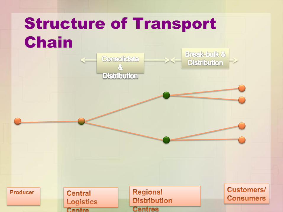
Structure of Transport

Chain

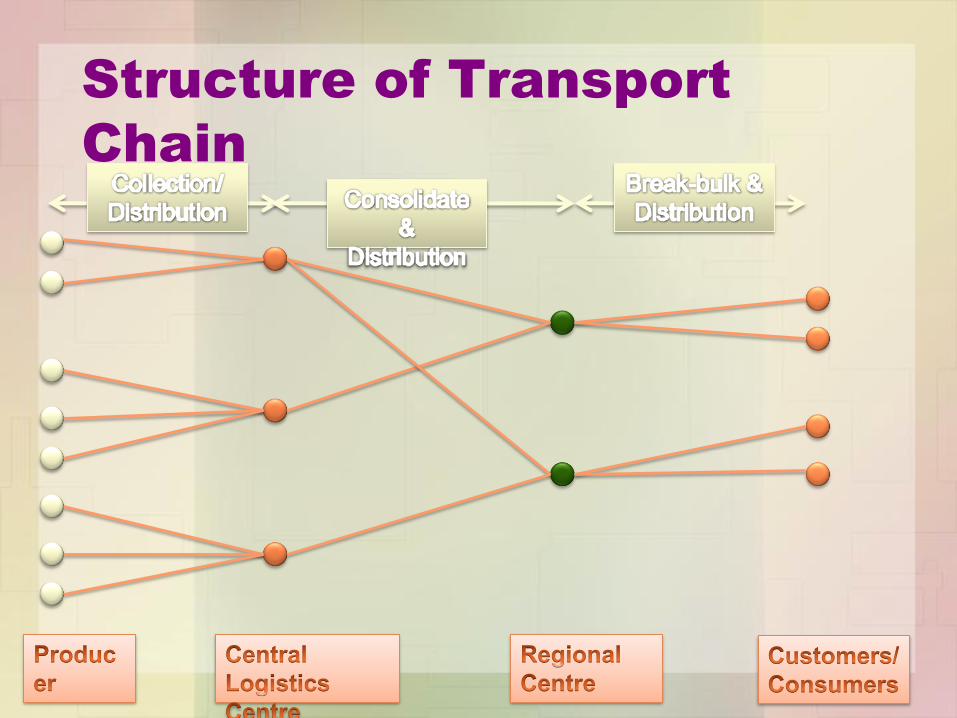
Structure of Transport

Chain

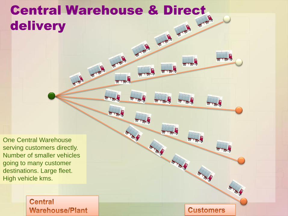
Central Warehouse & Direct

delivery

One Central Warehouse

serving customers directly.

Number of smaller vehicles

going to many customer

destinations. Large fleet.

High vehicle kms.

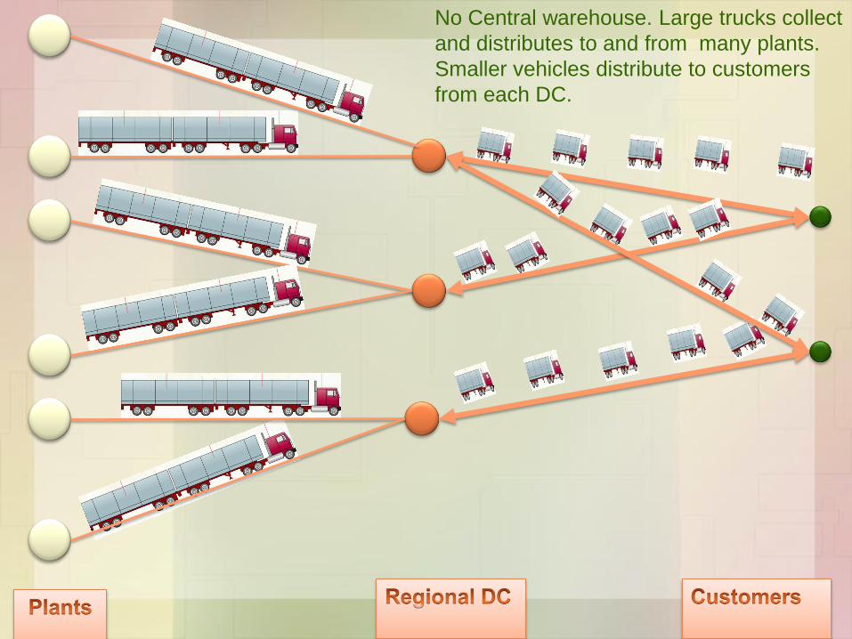
No Central warehouse. Large trucks collect

and distributes to and from many plants.

Smaller vehicles distribute to customers

from each DC.

No warehouses or DCs. Each

location is a cross docking where

trucks bring and distribute after

sorting out. (Lunch carrier operation

or vegetable distribution).

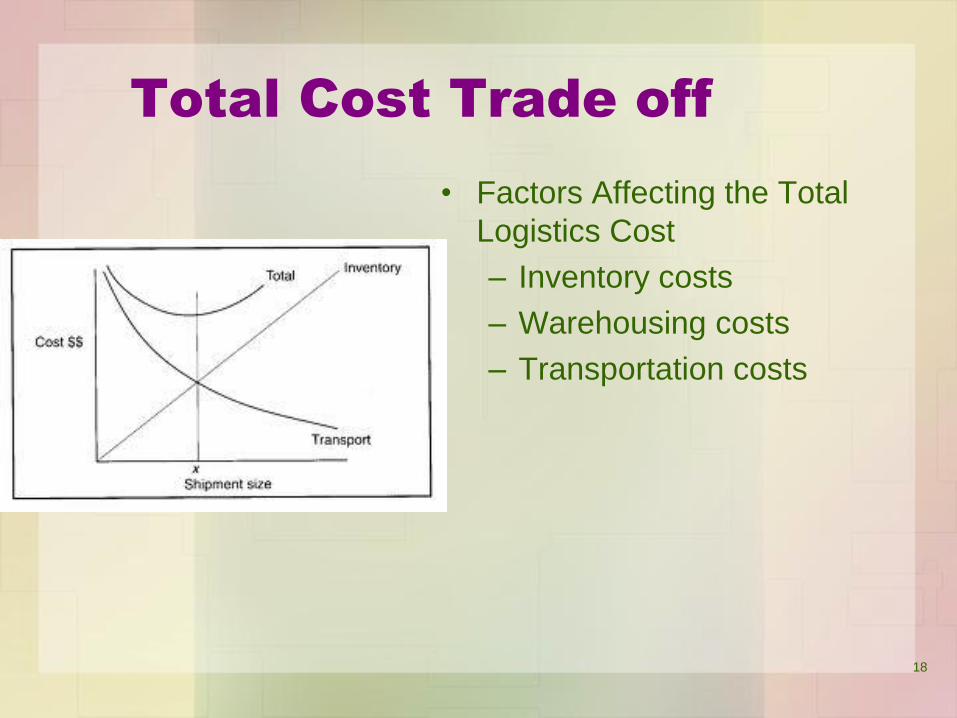
Total Cost Trade off

• Factors Affecting the Total

Logistics Cost

– Inventory costs

– Warehousing costs

– Transportation costs

18

Network Planning

Techniques for

Managing Transport

Operations Effectively

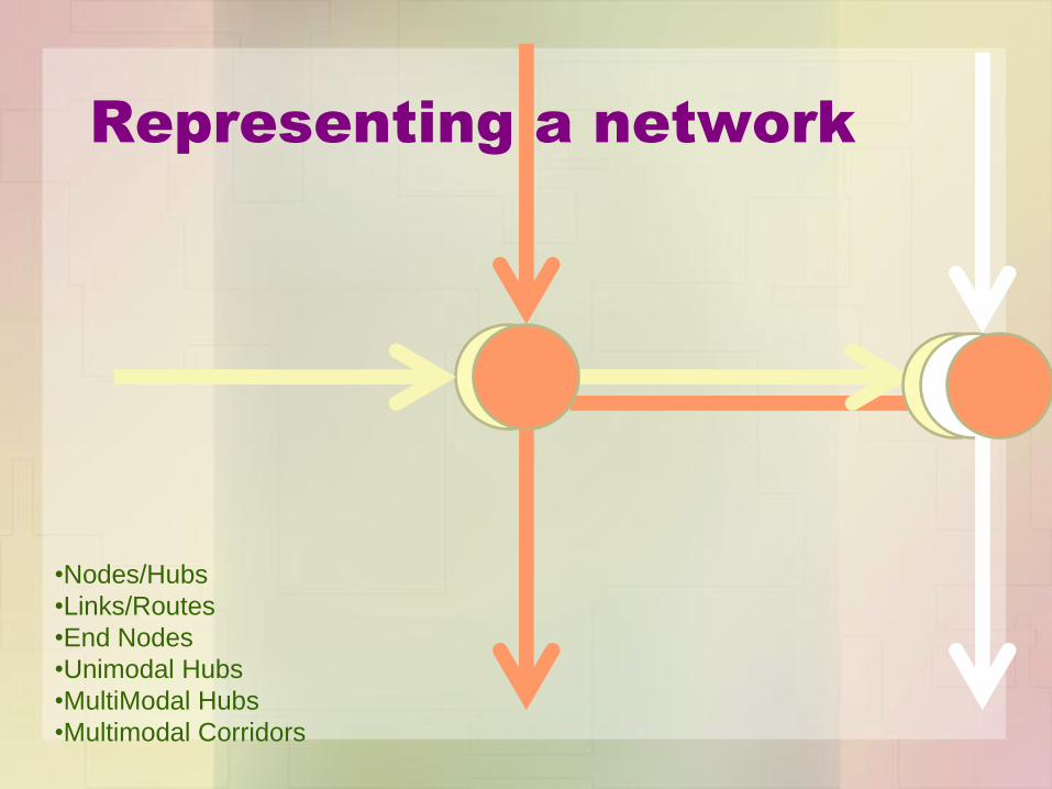
Representing a network

•Nodes/Hubs

•Links/Routes

•End Nodes

•Unimodal Hubs

•MultiModal Hubs

•Multimodal Corridors

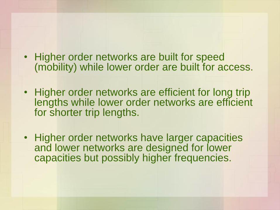
• Higher order networks are built for speed (mobility) while lower order are built for access.

• Higher order networks are efficient for long trip lengths while lower order networks are efficient for shorter trip lengths.

• Higher order networks have larger capacities and lower networks are designed for lower capacities but possibly higher frequencies.

Network Integration

Types of Networks

• Collection Networks (Many collect pointsone distribution point)

Examples

– Tea/Milk Collection

• Distribution Networks (One collect pointmany distribution points)

Examples

– Cement/Coca Cola

– Choon Paan/Newspaper

• Collector-Distributor Networks (many collect pointsmany distribution points)

Examples

– Courier

– School Vans/Office Vans

– Local route bus

• Point to Point Networks (one collect pointone distribution point

– Non-stop airline

– Dedicated Home delivery (Pizza)

– Chartered Services

Routing

• Fixed Route and Stops – Airlines

– Trains

– Milk Runs

• Fixed Route with Variable Stop – Buses

– Vegetable/Tea Leaf Pick up

• Route and Stops varied on demand – Courier service

– Office/School Van Service

• Point to Point

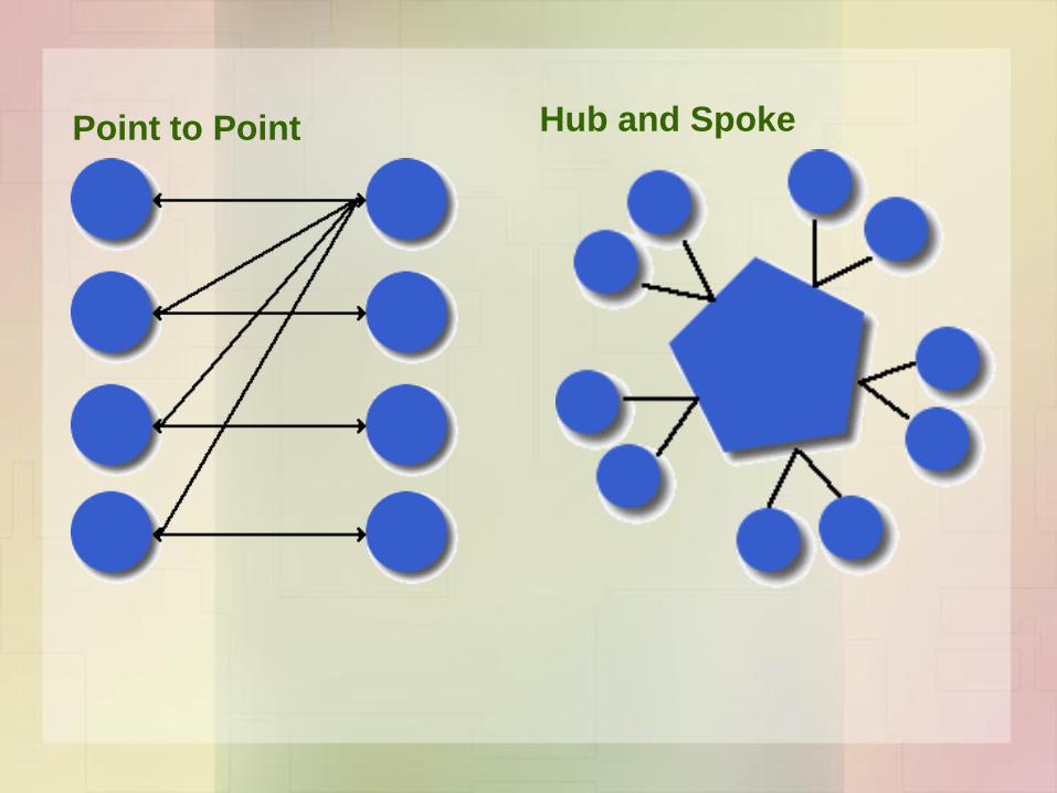
Point to Point Hub and Spoke

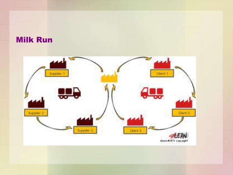
Milk Run

Vasiliauskas A.V., Modelling of National Multimodal Transport Networks,

Transport and Telecommunication,, Vol 4, N4, 2003

Strategic Network Planning

• At strategic level or long term level we

consider the planning of the underlying

physical network or infrastructure.

• The questions at Strategic Level are:

– Where the facilities should be located? (e.g.

where depots, warehouses should be built?)

– What resources should be acquired (e.g. what

type of truck to operate)?

– What type of services should be offered?

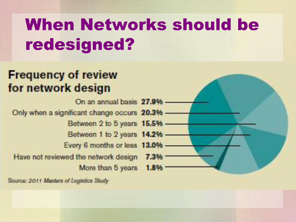
When Networks should be

redesigned?

Network Planning at Tactical Level

• At tactical level (medium term) we do not consider

the day-to-day operation of the network or facility,

but aggregate information to determine an efficient

and rational allocation of existing resources.

• Network planning and design problems at this level

are:

– Which customers to service?

– The capacity and frequency for each customer

– The positioning of empty vehicles? (what do I do with off

peak or off season capacity)

Operational Level

• Network planning and design problems at operational level are mostly involved in service delivery.

• For example a courier company needs to each day plan its routing, vehicles, personnel to use the underlying transportation network as cost efficiently as possible, at the same time ensuring that all deliveries are made on time.

Issues in Network Operational

Planning

• Scheduling fleet, staff to meet

anticipated demand.

• Planning to meet demand variations

• Recovering from events and incidents

• Determining service-cut off levels vs

minimum service levels

Network Operational Planning

• A network can be understood by its key operational features.

Some of the important features are:

• Time – from the user perspective door to door time is

important. For passenger travel, waiting time, transfer time

are more important. Overall journey speed determines the

journey time which includes stops, delays, transfers etc.

• Distance – determining minimum distance is important since

cost and speed are often associated with distance. It can also

mean higher costs.

• Capacity – the capacity determines the volume that can be

transported. Less volumes mean lower frequencies and lower

speeds. Capacity can be measured in terms of passengers,

vehicles or by weight or size.

Network Operational Planning

• Costs- The above translates to cost of carriage both in

terms of out of pocket cost and perceived cost. It also includes external social costs for which the user may or may not pay.

• Reliability - the ability to deliver on time repeatedly, measure as on time arrival.

• Transferability – the ability to transfer to other modes that are faster or cheaper at key points defined also as inter-modality.

• Quality – this refers to the quality that the user may require. Different services are provided with different qualitative aspects such as comfort, convenience, reliability, customer service, choice of service class etc.

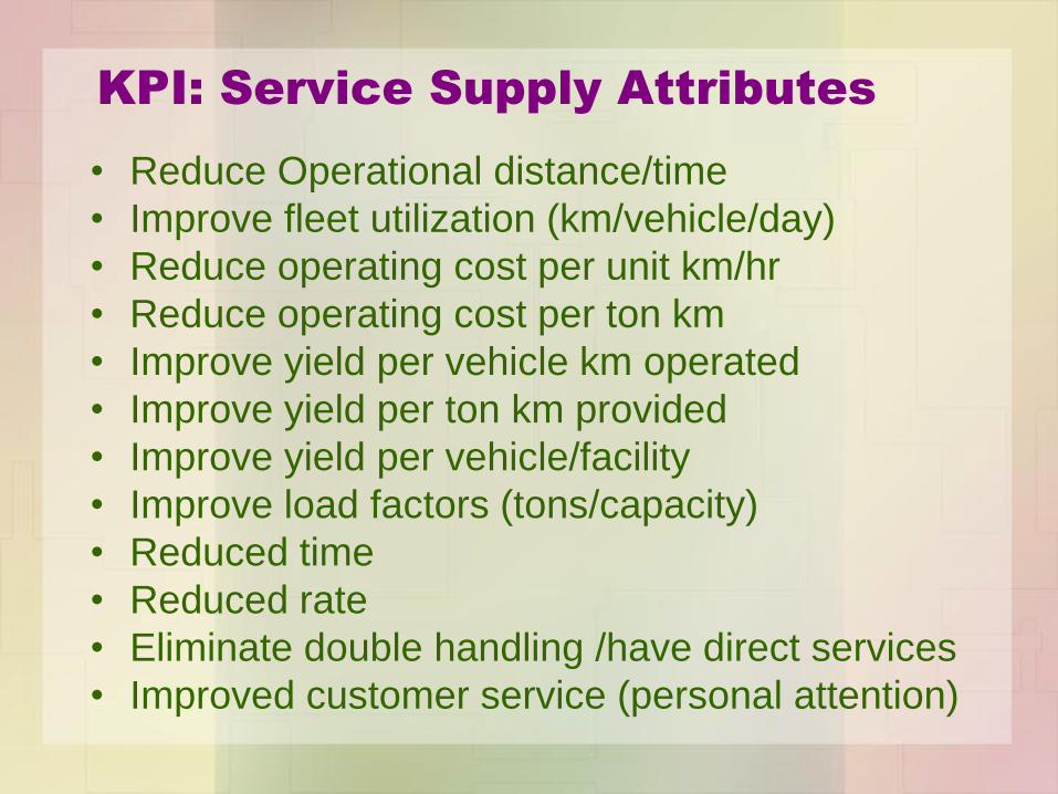
KPI: Service Supply Attributes

• Reduce Operational distance/time

• Improve fleet utilization (km/vehicle/day)

• Reduce operating cost per unit km/hr

• Reduce operating cost per ton km

• Improve yield per vehicle km operated

• Improve yield per ton km provided

• Improve yield per vehicle/facility

• Improve load factors (tons/capacity)

• Reduced time

• Reduced rate

• Eliminate double handling /have direct services

• Improved customer service (personal attention)

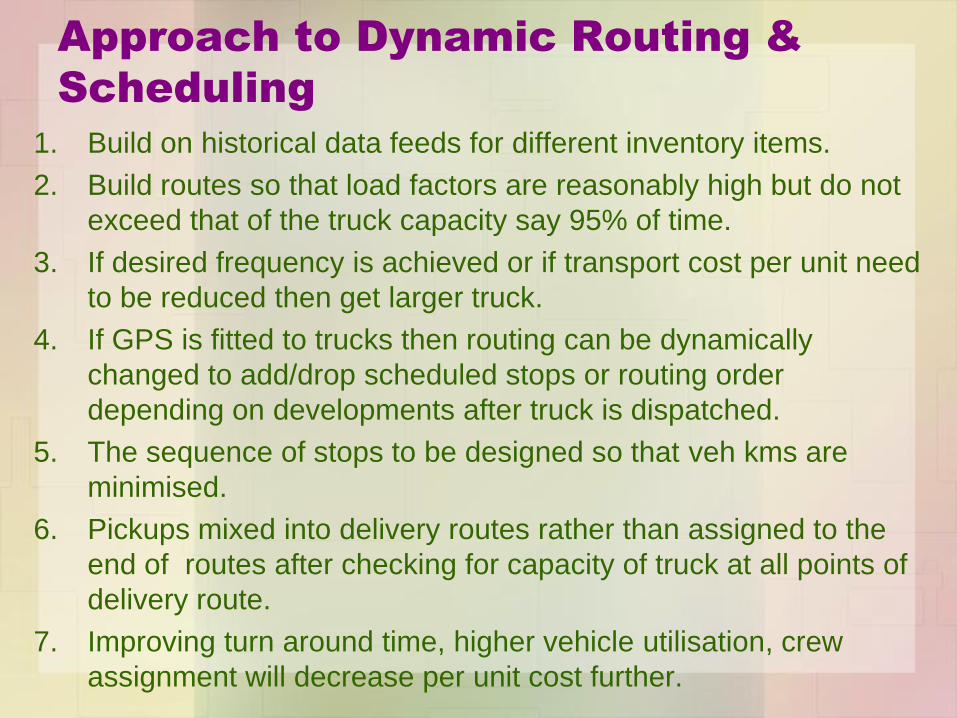
Approach to Dynamic Routing &

Scheduling

1. Build on historical data feeds for different inventory items.

2. Build routes so that load factors are reasonably high but do not

exceed that of the truck capacity say 95% of time.

3. If desired frequency is achieved or if transport cost per unit need

to be reduced then get larger truck.

4. If GPS is fitted to trucks then routing can be dynamically

changed to add/drop scheduled stops or routing order

depending on developments after truck is dispatched.

5. The sequence of stops to be designed so that veh kms are

minimised.

6. Pickups mixed into delivery routes rather than assigned to the

end of routes after checking for capacity of truck at all points of

delivery route.

7. Improving turn around time, higher vehicle utilisation, crew

assignment will decrease per unit cost further.

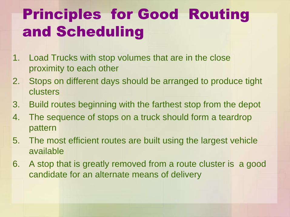
Principles for Good Routing

and Scheduling

1. Load Trucks with stop volumes that are in the close

proximity to each other

2. Stops on different days should be arranged to produce tight

clusters

3. Build routes beginning with the farthest stop from the depot

4. The sequence of stops on a truck should form a teardrop

pattern

5. The most efficient routes are built using the largest vehicle

available

6. A stop that is greatly removed from a route cluster is a good

candidate for an alternate means of delivery

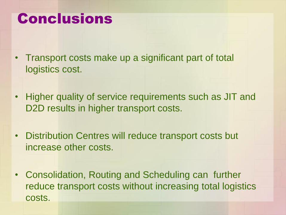
Conclusions

• Transport costs make up a significant part of total

logistics cost.

• Higher quality of service requirements such as JIT and

D2D results in higher transport costs.

• Distribution Centres will reduce transport costs but

increase other costs.

• Consolidation, Routing and Scheduling can further

reduce transport costs without increasing total logistics

costs.

Understanding the Cost

Profiles of Road Freight

Transport Services

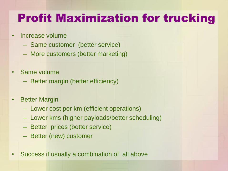
Profit Maximization for trucking

• Increase volume

– Same customer (better service)

– More customers (better marketing)

• Same volume

– Better margin (better efficiency)

• Better Margin

– Lower cost per km (efficient operations)

– Lower kms (higher payloads/better scheduling)

– Better prices (better service)

– Better (new) customer

• Success if usually a combination of all above

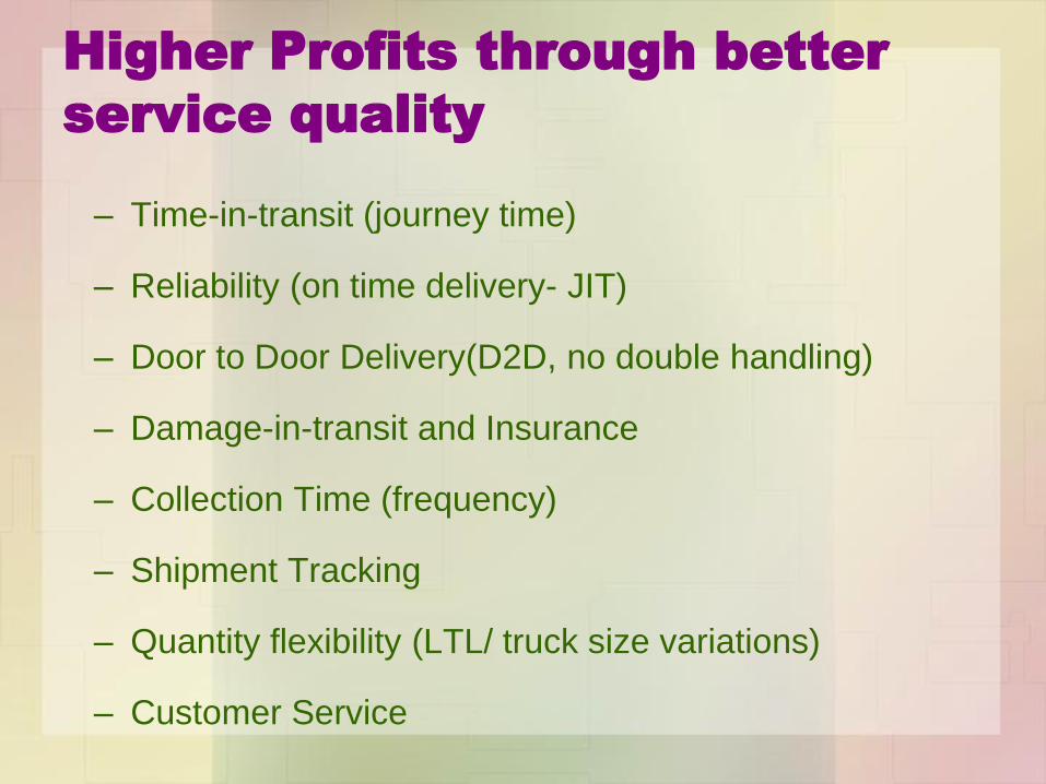
Higher Profits through better

service quality

– Time-in-transit (journey time)

– Reliability (on time delivery- JIT)

– Door to Door Delivery(D2D, no double handling)

– Damage-in-transit and Insurance

– Collection Time (frequency)

– Shipment Tracking

– Quantity flexibility (LTL/ truck size variations)

– Customer Service

Higher profits through

Lower Cost per km

The process

• Identify cost inputs

• Identify how input costs vary

• Reduce input volumes

• Reduce input unit costs

Variants of Truck

Operation Costs

• Type of Route (urban, low

country, up country)

• Type of Service (general cargo,

flat bed, bowser)

• Tare (maximum carrying

capacity, tonnes, litres)

• Age of Truck

• Country of Origin (Technology)

– Indian, Chinese, Japanese,

European

• Trip Type (short haul, long haul)

• Working Hours (regular, single

shift with OT, double shift)

• Truck availability for operation

(days/month)

• Average kms operated/month

• Percentage empty running

• Percentage dead running

• Average Load Occupancy

• ICT applications

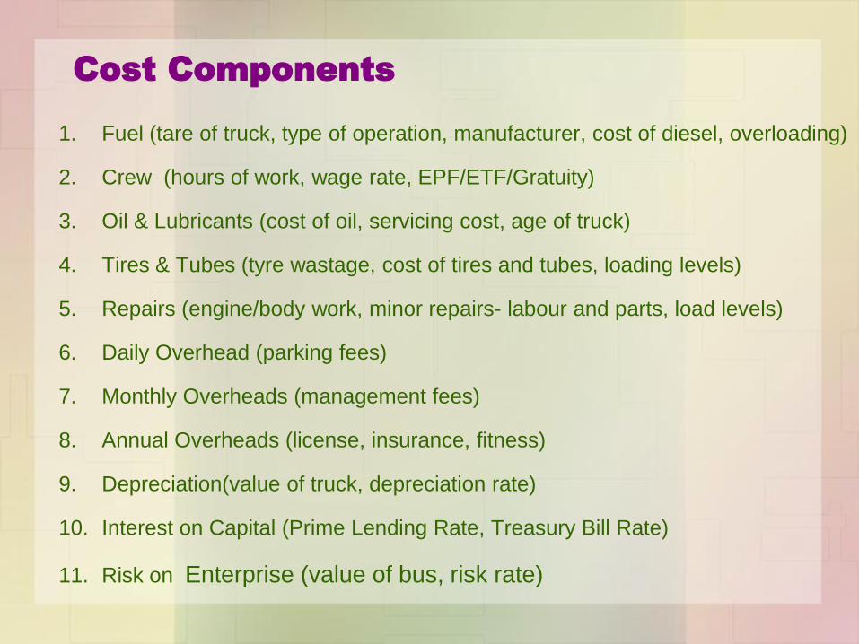
Cost Components

1. Fuel (tare of truck, type of operation, manufacturer, cost of diesel, overloading)

2. Crew (hours of work, wage rate, EPF/ETF/Gratuity)

3. Oil & Lubricants (cost of oil, servicing cost, age of truck)

4. Tires & Tubes (tyre wastage, cost of tires and tubes, loading levels)

5. Repairs (engine/body work, minor repairs- labour and parts, load levels)

6. Daily Overhead (parking fees)

7. Monthly Overheads (management fees)

8. Annual Overheads (license, insurance, fitness)

9. Depreciation(value of truck, depreciation rate)

10. Interest on Capital (Prime Lending Rate, Treasury Bill Rate)

11. Risk on Enterprise (value of bus, risk rate)

Factors for Fuel Efficiency of Trucks

Source: Kenworthy- Trucking

Fuel Consumption Euro III 17

tonne truck

Source: Transport Research Laboratory,- www.trl.co.uk

y = -4E-05x3 + 0.009x

2 - 0.6665x + 20.652

R2 = 0.8574

0

5

10

15

20

25

0 20 40 60 80 100 120 140

Average speed (km/h)

Fu

el

Co

ns (

l/100km

)

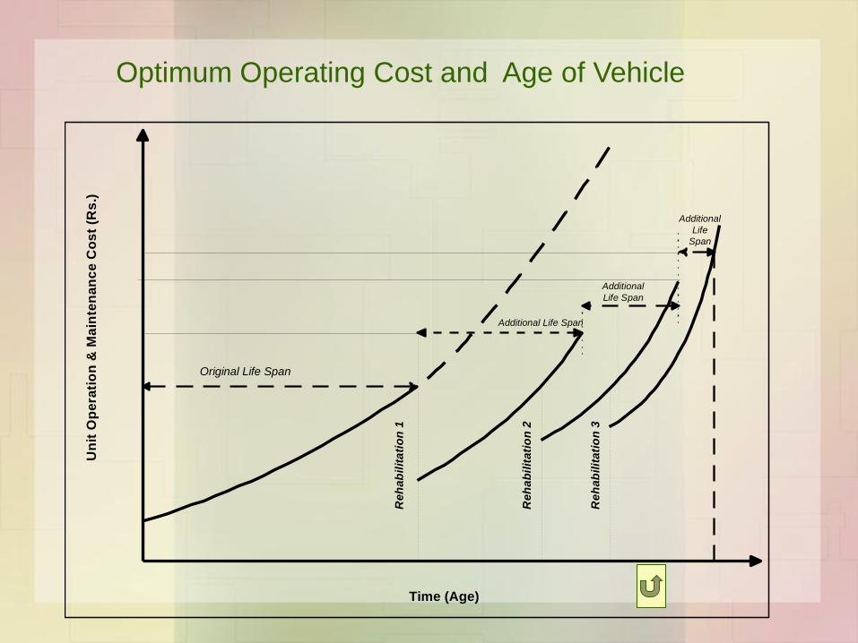
Re

ha

bil

ita

tio

n 1

Re

ha

bil

ita

tio

n 2

Re

ha

bil

ita

tio

n 3

Additional Life Span

Additional

Life Span

Additional

Life

Span

Time (Age)

Original Life Span

Un

it O

pe

rati

on

& M

ain

ten

an

ce

Co

st

(Rs

.)Optimum Operating Cost and Age of Vehicle

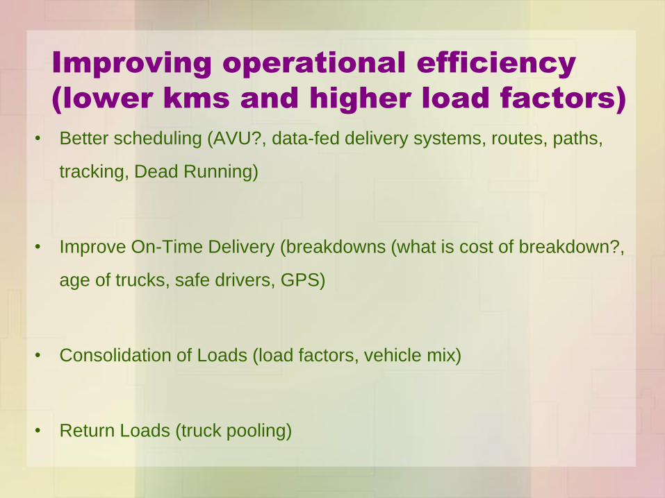
Improving operational efficiency

(lower kms and higher load factors)

• Better scheduling (AVU?, data-fed delivery systems, routes, paths,

tracking, Dead Running)

• Improve On-Time Delivery (breakdowns (what is cost of breakdown?,

age of trucks, safe drivers, GPS)

• Consolidation of Loads (load factors, vehicle mix)

• Return Loads (truck pooling)

Some key solutions- and take home lessons

• Reducing cost and improving output quality the

most important factors for profitability

• To reduce costs you should identify cost factors

and know what causes them to vary

.

• The mix at which the lowest cost is achieved with

the best output of quality will provide the best

profitability in the long run.