1  

Information Asymmetry and Bank Regulation:

Can the Spread of Debt Contracts be explained by Recovery Rate?1

Wenchien Liu

Department of Finance

National Chengchi University

Peter Miu

DeGroote School of Business

McMaster University

Yuanchen Chang

Department of Finance

National Chengchi University

Bogie Ozdemir

BMO Financial Group

Abstract

We investigate whether the spread of corporate debt contacts can be explained by

their ultimate recovery rates. Using the actual realized recovery rates of defaulted

debt instruments issued in the U.S. from 1962 to 2007, we find that recovery rate is

reflected in the spread at issuance, and their relationship has become more significant

since commercial banks were allowed to underwrite corporate securities. Using

various market microstructure and firm-level opaqueness measures, our further

investigation indicates that the enhanced informativeness of recovery rate can be

attributed to the lowering of information asymmetry. Besides, the relation between

the spread at issuance and the recovery rate is stronger for weak corporate governance

and non-investment grade issuers. Our conclusions are found to be robust to

endogeneity issues, potentially omitted variables and alternative model specifications.

JEL classification: G10; G11; G12; G13; C5

Keywords: Recovery risk; Information asymmetry; Bank regulation; Corporate

governance; Credit rating; Glass-Steagall Act; Financial Modernization Act

                                                       1  The  former  title  is  “Is  Recovery  Risk  Priced  in  Debt  Contracts?  The  Roles  of  Bank  Regulation, Corporate Governance and Credit Rating”. 

2  

The old proverb says that “Half a loaf is better than none”, which maybe the best

description for all creditors as firms go bankruptcy.

1. Introduction

Debtholders encounter both default and recovery risk. The former could be

measured by the probability of default of the issuer; whereas the latter refers to the

chance of recovering less than the full amount of principal plus interests given the

occurrence of the default event. Those debt instruments which are perceived having

a higher (lower) probability of default and lower (higher) recovery rate should

command a higher (lower) spread.2 This paper examines whether the spreads of the

debt contracts at the time of issuance can be explained by the realized recovery rates

at the time of default. We find that both information asymmetry and bank regulation

have important effects on how much recovery rate information are reflected in the

spread at issuance.

Information asymmetry exists between the lender and the borrower of a

corporate debt contract. By restricting the financial activities of the borrower, debt

covenants could mitigate some of the effects of information asymmetry. Theoretically,

the degree of information asymmetry of a debt contract is reflected in its issuance

price (i.e. its spread). The lower the information asymmetry, the lower is the spread

charged by the lender. Besides, a lower information asymmetry can also ensure the

inherent risks of the contract are more accurately reflected in its spread. Spread can

thus be more effectively explained by the realized recovery rate.

Given the characteristics of the corporate loan contracts, commercial banks

command an information advantage over non-bank investors on the financial health of

                                                       2 Recovery rate is the proportion of the amount of principal plus accrued interests being recovered

during the workout process of a default event.

3  

their corporate clients.3 Such information could be effectively revealed to non-bank

investors in underwriting the corporate bonds and equities issued by their clients.

This “certification effect” (as formally modeled by Puri, 1999) could therefore lower

the information asymmetry of the capital markets. However, allowing commercial

banks to underwrite bonds and equities issued by their clients may result in a potential

conflict of interest. Banks have financial incentive to promote securities issued by

their clients of doubtful credit quality while using the proceeds from the issuance to

retire the outstanding bank loans. To avoid this potential conflict of interest, the

1933 Glass-Steagall Act forbade U.S. commercial banks from underwriting corporate

securities. The results of empirical studies (e.g. Puri, 1994, 1996), based on data of

debt instruments from the pre-Glass-Steagall Act era, are however more consistent

with the certification effect than suggesting the conflict of interest being exploited by

commercial banks.

Studies conducted after the relaxation of Section 20 of the 1933 Glass-Steagall

Act, allowing (on a case-by-case basis) commercial banking subsidiaries to participate

in the underwriting of corporate bonds and equities, also support the certification

effect of commercial banks.4 For example, Gande et al. (1999) show that those debt

instruments which were underwritten by commercial banks tend to be issued at a

higher price (i.e. a lower yield). By comparing the long-run returns of IPO equity

issues underwritten by “relationship banks” and “independent banks”, Benzoni and

Schenone (2010) also find support of the certification role of commercial banks.

                                                       3 Through continuous monitoring and dialogue with senior management in a corporate loan relation,

commercial banks could extract timely information on the debt issuer at relatively low costs. 4 In 1987, the Federal Reserve gave the first permission to a bank to underwrite commercial paper and

municipal bonds. Subsequently, the first corporate bond and equity underwritings were permitted in

1989 and 1990 respectively. Eventually, the passing of the Financial Modernization Act in 1999

removes all the barriers for commercial banks to participate in the underwriting business.

4  

To contribute to the literature, this paper examines the regulatory impact by

investigating whether credit spreads at the time of issuance can be explained by

ultimate recovery rates at the time of default. Specifically, we want to find out if the

explanatory power of recovery rate has been strengthened after commercial banks are

allowed to underwrite corporate securities. Our approach in addressing the issue is

therefore different from those in the previous studies, in which the costs and benefits

of allowing commercial banks to underwrite debt contracts are investigated by

considering either the ex-ante bond prices at issuance (e.g. in Puri, 1996) or the

ex-post performances based on realized default rates (e.g. in Kroszner and Rajan,

1994; and Puri, 1994). We examine the certification effect (or the lack thereof) by

measuring how much recovery rate information are reflected in the spread at issuance.

We therefore focus our attention on the defaulted debt contracts. It is the subsample

of the universe of debt instruments that ever results in realized losses to the lenders.

We believe, by conducting our analysis with this subsample, it will yield the most

fruitful results to our research questions.

The gradual relaxation of the Glass-Steagall Act (i.e. the partial relaxation of

Section 20 and the complete removal of the barrier by the Financial Modernization

Act in 1999) provides a perfect historical setting for us to gauge the impact of bank

regulation on information asymmetry in the debt markets. It will be consistent with

the certification effect if realized recovery rate becomes more accurately reflected in

the spread at issuance after commercial banks were gradually allowed to participate in

the underwriting business.

Finally, we also examine the role of the economics of collecting and process

information on the credit worthiness of the debt issuers. A lender will only collect

such information if the related costs can be covered by the expected marginal benefit

brought about by such information. We consider characteristics of the issuer which

5  

might dictate the perceived benefit of acquiring information on its inherent recovery

risks. Specifically, issuers of good corporate governance and of investment grade

are perceived to be of low probability of default, and thus the benefit of finding out

how much could be recovered from a defaulted event tends to be small. Without the

incentive of possessing information on recovery risks, it would not be surprising that

recovery rate information cannot be accurately reflected in the spread of the debt

contracts issued by these types of borrowers.

The rest of this paper is organized as follow. In Section 2, we review the

literatures and illustrate the four hypotheses. In Section 3, we describe the data used

in our empirical study and present a number of summary statistics. The main

empirical results are reported in Section 4. In Section 5, we conduct a number of

analyses to gauge the robustness of our conclusions. We finally conclude with a few

remarks in Section 6.

2. Literature Review and Hypotheses

The pricing of default risks has been well studied.5 In this study, we examine

whether recovery risk is reflected in spreads after controlling for the cross-sectional

difference in default risks. Previous empirical studies on the pricing of recovery

risks are mixed. The findings of Bakshi et al. (2006) suggest that recovery rates are

considered in the pricing of corporate bonds. Elton et al. (2001) investigate the

significance of expected default loss, tax premium and risk premium in explaining the

variation of corporate bonds spread. Their results however suggest that expected

default loss, as a proxy for recovery risk, has very limited explanatory power. Using

                                                       5 See for example Collin-Dufresne et al. (2001), Elton et al. (2001), Eom et al. (2004), and Driessen

(2005).

6  

the return on S&P’s 500 to control for the variation of recovery rates, Collin-Dufresne

et al. (2001) study the determinants of credit spread changes. They conclude that it

is the local supply/demand shocks, rather than credit risk or liquidity risk factors, that

have the highest explanatory power.

The reason for these mixed results could be due to the fact that it is difficult to

find a good proxy for recovery risk. The findings of Altman et al. (2004, 2005) and

the literature survey of Altman et al. (2005) indicate that recovery rate is governed by

not only systematic factors, but also industry-specific and firm-specific factors. The

explanatory power could therefore be limited if only a systematic factor (e.g. the

return on S&P’s 500 in Collin-Dufresne et al., 2001) is used to proxy for recovery rate.

The difficulty in obtaining an ex-ante measure of recovery rate could be the second

reason for the mixed results. With the growth of the credit derivatives markets,

recovery rates implicit in the market prices of credit derivatives can be used as ex-ante

measures of recovery rates (Berd, 2005, Das and Hanouna, 2009). Historical pricing

information of credit derivatives in the 80s and 90s are however quite limited, which

presents a challenge in using it for empirical research involving historical period that

extends to earlier than the last decade.

In this study, rather than using recovery rate proxies or ex-ante estimates of

recovery rates, we consider the ex-post realized recovery rates of the debt instruments.

We focus on those debt instruments which have already defaulted and examine if the

actual realized recovery rates were indeed reflected in the spreads when they were

initially issued. If recovery risk is indeed a determinant of the price of the debt

contract, the ex-post value of recovery rate should be positively (negatively) related to

the issuance price (spread). This gives us our first hypothesis.

H1: “Credit spread at the time of issuance is negatively related to

the realized recovery rate at the time of default.”

7  

One of the focuses of this study is to examine the impact of bank regulations on

information asymmetry and how it might affect the processing of recovery rate

information in the pricing of corporate debts at issuance. Specifically, we consider

changes across the three legislative regimes of gradual relaxation of the restriction of

commercial banks in underwriting corporate bonds and equities. Given the

information advantages and economies of scope of commercial banks, the opening of

the underwriting market can reduce the information asymmetry between issuers and

non-bank investors.6 This is essentially the certification effect demonstrated by Puri,

(1994, 1996), and Gande et al. (1997). The reduction of information asymmetry

should therefore lead to a stronger relation between spread and recovery rate when

commercial banks are gradually allowed to participate in underwriting corporate

bonds. Based on the above, we have our second hypothesis.

H2: “There is no significant relation between spread and recovery

rate before 1989 when the Glass-Steagall Act was in full

force. The relation between spread and recovery rate starts

to become significant between 1989 and 1999 when

commercial banks were gradually allowed to set up Section

20 subsidiaries to underwrite corporate instruments. The

relation is the strongest after 1999 when the underwriting

market is fully opened with the passing of the Financial

Modernization Act”

With the benefit of having observations after the passing of the Financial

Modernization Act in 1999, we have the complete picture of the effect of the complete

liberalization of the underwriting business which was not previously available to

                                                       6 See literature survey by Gande (2008).

8  

Gande et al. (1999).

In formulating our second hypothesis, we attribute the impact brought about by

the changes in the bank regulation to the lowering of information asymmetry. We

can therefore further verify this hypothesis by directly assessing the impact of

information asymmetry on the relation between spread and recovery rate. We would

expect any direct proxies for information asymmetry characterizing the issuer will

play an important role in affecting this relation. Specifically, the lower the

information asymmetry, the stronger is this relation. We consider three different

direct proxies for information asymmetry: (a) the information asymmetry index of

Bharath et al. (2009) based on market-microstructure information; (b) public verse

private firms (Sufi, 2007); and (c) the degree of asset specificity (Acharya et al.,

2007).7

In addition to examine the impact of bank regulation on the pricing recovery risk,

we also consider the role played by the quality of corporate governance of the

borrower in the relation between spread and recovery rate. The better the corporate

governance of the borrower, the lower is the marginal benefit for creditors to process

information on recovery rate at the issuance of the debt contract given the lower

perceived probability of default.8 It is therefore not cost effective for creditors to

accurately assess the recovery rate of these instruments, and thus recovery rate

information is less reflected in the spread at issuance. The same argument can be

made for debt contracts issued by investment grade (as opposed to non-investment

                                                       7 The more specific the asset of a firm, the less transparent it is, and thus the more information

asymmetry exists between the firm and its outside investors (and financial intermediaries). 8 In this study, the quality of corporate governance is measured by examining the anti-takeover

provisions of the debt issuers. We consider the Governance Index (G-Index) of Gompers et al. (2003),

which counts the number of anti-takeover provisions (a maximum of 24). The more anti-takeover

provisions (higher G-Index), the worse is the corporate governance of the company, and thus the higher

is the chance of having any agency problems.

9  

grade) borrowers. Again, given that the probability of default is perceived to be low

for investment grade firms, creditors pay less attention in assessing recovery rate

information which is only relevant subsequent to an (unlikely) default event. We

therefore have our third and fourth hypotheses.

H3: “The relation between spread and recovery rate is weaker

(stronger) for those debt instruments issued by borrowers

with better (worse) corporate governance.”

H4: “The relation between spread and recovery rate is weaker

(stronger) for those debt instruments issued by investment

grade (non-investment grade) borrowers.”

Moreover, allowing commercial banks to participate in the underwriting business

should be able to lower the cost of information, thus providing incentives for creditors

to process information on recovery rate even for borrowers with good corporate

governance or of investment grade. It could therefore result in a stronger relation

between spread and recovery rate for these borrowers after the legislative barrier is

removed. However, the increase in competition for underwriting business

subsequent to the liberalization could give us the opposite result (e.g., Shivdasani and

Song, 2010). Underwriters might sacrifice a thorough assessment of the inherent

risk of the borrower for the sake of winning the mandate of placing the debt. We

would expect such negative effect of competition being more pronounced when the

issuers are perceived to be of relatively better corporate governance or the issuers are

of investment grade. Underwriters think that the chance of running into a “bad deal”

is quite small for these borrowers and thus willing to assume the reputation risk. The

heightening of competitions subsequent to the opening of the underwriting business

might therefore result in recovery rate information being less effectively reflected in

the spreads for borrowers of better corporate governance or for investment-grade

10  

borrowers.

Finally, the effect of the relaxation of Glass-Steagall Act is expected to be

stronger for those debt contracts issued by borrowers which are deemed to be more

prone to information asymmetry, thus having a “higher demand of certification”.

Given that public information on non-investment grade borrowers are in general less

readily available than that of investment-grade ones, the former have a higher demand

of certification.9 We therefore expect the effect of the relaxation of the Act on the

relation between spread and recovery rate for non-investment grade debts to be

stronger than that on investment grade debts.

3. Data Description, Variables Definition and Summary Statistics

We obtain the recovery rates of defaulted debt instruments from Standard &

Poor’s (S&P's) LossStats Database. Recovery rate is expressed as dollar amount

recovered per $1,000 notional value of the defaulted debt instrument. It is computed

by discounting the ultimate recovery values back to the time of default. Ultimate

recovery value is the value pre-petition creditors would have received had they held

onto their position from the point of default through the emergence date of the

restructuring event. 10 , 11 This database represents a comprehensive set of

                                                       9 For example, Puri (1996) documents a significant difference in yields between bank-underwritten

and investment-house-underwritten issues for non-investment grade but not for investment-grade

instruments.

10 Pre-petition creditors are creditors that were in place prior to filing a petition for bankruptcy. 11 Ultimate recovery values of the defaulted debts are calculated in the LossStats Database by one of

three methods: (1) emergence pricing - trading price of the defaulted instrument at the point of

emergence from default; (2) settlement pricing - trading price at emergence of those instruments

received in the workout process in exchange for the defaulted instrument; and/or (3) liquidity event

pricing - values of those instruments received in settlement at their respective liquidity events (e.g.

11  

commercially assembled credit loss information on defaulted loans and bonds.

Public and private companies, both rated and non-rated, that have bank loans and/or

bonds of more than fifty million dollars are analyzed and included in the database.12

The companies must have fully completed their restructuring, and all recovery

information must be available in order to be included.13 We examine the recovery

information on defaulted debt instruments issued from February 1962 to March 2007.

Out of these 3,682 debt instruments, there are 1,412 bank debts, 341 senior secured

bonds, 957 senior unsecured bonds, 506 senior subordinated bonds, 413 subordinated

bonds, and 53 junior subordinated bonds. These instruments are from 790 separate

company default events occurring from March 1985 to October 2007, and from a

variety of industries.

The summary statistics of the discounted recovery rates (Recovery Rate) of the

full sample of defaulted debt instruments are reported in Panel A of Table 1. We

express Recovery Rate as a proportion of the notional value (i.e., recovery value per

$1 notional value). The full sample average of recovery rate is 0.555. Judging

from the standard deviation of 0.380, the variability of recovery rate is quite

substantial. Panels B, C, and D of Table 1 present the summary statistics of three

subsamples based on the date of issuance of the debt contract. They correspond to

the three subperiods of the legislative regimes, namely: (i) Before 1989: when

commercial banks were forbidden to participate in the underwriting of corporate

                                                                                                                                                           

suppose creditors receive newly issued bonds during the settlement process; liquidation event prices are

the liquidation values of these bonds at their respective maturity dates). When possible, all three

methods are considered in the calculation of the recovery value of each instrument. Then, based on

additional information, the method that is expected to be most representative of the recovery

experience of the prepetition creditors was used to arrive at the recovery value. 12 Financial, real estate, and insurance companies are excluded. 13 Recovery information on bankruptcies, distressed exchanges, and other reorganization events, are

included.

12  

bonds and equities, (ii) After 1989 but before 1999: when commercial banks were

gradually allowed to set up Section 20 subsidiaries to underwrite bonds and equities,

and (iii) After 1999: when the underwriting market is fully opened to commercial

banks with the passing of the Financial Modernization Act. Recovery rate is, on

average, increasing throughout these three time periods.

Besides the information on recovery rate, we also collect the following

information on the defaulted instruments and their issuers from the LossStats

Database, S&P's Compustat, the Center for Research in Security Prices (CRSP), and

the Investor Responsibility Research Center (IRRC).

o Spread: the spread (in percent) of the instrument at issuance over LIBOR,

prime rate, or Treasury rate. It is obtained from LossStats.

o Rating: S&P's long-term issuer credit rating (from Compustat) in the year of

issuance of the debt instrument. We construct this variable by converting the

S&P's letter grade of AA+, AA, AA-, etc., into numerical values of 1, 2, 3, etc.,

respectively.

o Maturity Days: the maturity of the debt contract, which is defined as the

difference (measured in number of days) between the maturity date of the

contract and its issuance date. The data source is also from LossStats.

o Ln(Amount): the natural log of the original issue amount (in dollars) from

LossStats.

o Default Probability: is the default probability measure of Bharath and

Shumway (2008). In calculating this variable, we obtain the required

financial statement information from S&P's Compustat and stock market

information from CRSP.

o Volatility: equity return volatility is defined as the standard deviation (in

percent) of daily excess return of the borrower’s equity value over the 180

13  

days prior to the issuance of the debt contract.14 Equity return information

are obtained from CRSP.

o Default Days: the number of days between the issuance and default date of the

debt contract obtained from LossStats.

o G-Index: is the corporate governance index of Gompers et al. (2003). We

obtain the corporate provision information from IRRC. More details are

provided in Section 4.4.

The summary statistics of the above variables are again reported in Table 1. Spread,

on average, is decreasing throughout the three time periods of legislative regimes.

<<Insert Table 1 about here>>

4. Empirical Results

In this section, we conduct a number of regression analyses to find out if there

are any empirical supports for the four hypotheses introduced in Section 1.

4.1 The relation between spread at issuance and realized recovery rate

We test our first hypothesis of whether the spread at the time of issuance is

negatively related to the realized recovery rate at the time of default by running a

number of ordinary least square (OLS) regressions using the spread of the debt

contract as dependent variable; whereas its corresponding (discounted) recovery rate

as independent variable. We start with the univariate regression of Equations (1).

Theoretically, the higher the expected recovery rate of the contract, the lower the

spread demanded by the creditors. A negative and statistically significant value of β1

will therefore support hypothesis H1.

                                                       14 We follow Campbell and Taksler (2003) in constructing this volatility measure.

14  

0 1 .Spread RecoveryRate (1)

The results are reported in Panel A of Table 2. Besides presenting the point

estimates of the coefficients, we also report the corresponding t-statistics after

correcting for heteroskedasticity using White’s (1980) variance-covariance matrix.

In Panel A, besides presenting the results for the full sample (labeled as “All Sample

Period” in Table 2), we also report the subsample results corresponding to the three

legislative regimes of the Glass-Steagall Act based on the dates of issuance of the

respective debt contracts.

<<Insert Table 2 about here>>

Let us first focus on the full sample results of Table 2 Panel A. The coefficient

of recovery rate is negative and statistically significant at the 1% confidence level in

explaining the spread at issuance, thus supporting our first hypothesis. In this

univariate setting and based on the point estimate of -4.673, an absolute increase in

recovery rate by ten percent is related to a reduction in the spread of about 47 basis

points (bps). Next, we conduct the multivariate regression of Equation (2), in which

we control for other contract-specific factors which might affect the spread at

issuance.

.8765

43210

sDefaultDayVolatilitybabilityDefaultProAmountLn

SICcodeysMaturityDaRatingteRecoveryRaSpread (2)

We consider the credit rating of the borrower (Rating) at the issuance of the debt,

which is defined as its Standard and Poor’s (S&P’s) long-term issuer credit rating.

15  

We construct this variable by converting the letter grade of AA+, AA, AA-, etc., into

numerical values of 1, 2, 3, etc., respectively.15 The summary statistics of this

variable are presented in Table 1. The higher the value of this variable, the lower is

the credit quality of the borrower. We therefore expect the spread is positively

related to this variable. We also control for the maturity of the debt contract

(Maturity Days), which is defined as the difference (measured in the number of days)

between the maturity date of the contract and its issuance date. A positive term

structure will result in a positive relation between the spread of the contract and its

time-to-maturity. Any industry-specific effects are catered for by considering the

4-digit SIC code (SIC Code) of the borrower. We also control for the size of the

issue amount by constructing the variable Ln(Amount), which is the natural log of the

original issue amount. Since debt contracts of larger issue amounts are likely to be

more liquid and convey more public information than those of smaller issue amounts,

spread is expected to be negatively related to Ln(Amount). We construct two other

borrow-specific variables to control for the variation of probability of default among

different borrowers. We compute the default probability measure (Default

Probability) of Bharath and Shumway (2008), which is evaluated based on the

“distance-to-default” of the borrower at issuance date. Another governing variable

according to the Merton’s model of default risk is the volatility of the borrower’s asset

value. We follow Campbell and Taksler (2003) and construct variable Volatility by

computing the standard deviation of daily excess return of the borrower’s equity value

over the 180 days prior to the issuance of the debt contract. It thus serves as the

proxy of the volatility of the borrower’s asset value. Finally, we also control for the

time-to-default (Default Days), which is the number of days between issuance and

                                                       15 The highest credit rating of the borrowers in our sample is AA+.

16  

default date of the debt contract. The results of this multivariate regression are

reported in Panel B of Table 2. Again, the t-statistics are corrected for

heteroskedasticity using White’s (1980) variance-covariance matrix.

Let us first consider the full sample results of Panel B of Table 2. After

controlling for the other explanatory variables of credit spread, recovery rate is still

statistically significant at 1% confidence level. Based on the point estimate of its

coefficient of -3.233, an absolute increase in recovery rate by ten percent is related to

a decrease of the spread by about 32 bps, which is slightly more than the decrease in

spread corresponding to a one-notch improvement in credit quality.16 Based on the

point estimate of 0.292 of the coefficient of Rating, a one-notch improvement in

credit quality according to S&P’s long-term issuer credit rating is related to a decrease

in the spread of about 29 bps. It is also statistically significant at 1% level. The

positive and statistically significant coefficient of Maturity Days is consistent with an

upward sloping term structure of credit spread. An increase in the maturity by one

year is related to an increase in the spread of about 11 bps (= 365 days × 0.000288 ×

100bps). Variables SIC Code and Ln(Amount) are found to be insignificant in

explaining the variation in spread. As expected, the dependent variable is positively

related to the default probability measure (Default Probability) of Bharath and

Shumway (2008) and it is statistically significant at 1%. The variable Volatility has

the expected sign, though it is not statistically significant. Finally, the coefficient of

Default Days is found to be positive and statistically significant, even though

instruments with larger spreads are expected to default sooner than those with smaller

spreads. Further investigations (not reported) suggest that we are likely capturing

the time effect of credit spread with the use of the variable Default Days. Both the

                                                       16 From Panel A of Table 1, the unconditional cross-sectional standard deviation of recovery rates of

our sample is about 38%.

17  

spread at issuance and the time to default (Default Days) tend to be decreasing over

time throughout our sample (see Table 1), thus resulting in a positive relation between

the dependent variable and Default Days.17

In summary, the full sample results of Table 2 support our first hypothesis.

Specifically, the lower the realized recovery rate, the higher the spread at issuance.

The relation is both statistically and economically significant, even after controlling

for other potentially confounding factors.

4.2 The relation between spread at issuance and realized recovery rate subsequent to

the gradual liberalization of the underwriting markets

To examine the validity of our second hypothesis, we repeat the OLS regressions

of Section 3.1, but on three different subsamples according to the dates of issuance of

the debt contracts, namely before 1989, from 1989 to 1999, and after 1999, which

respectively correspond to the legislative regimes of full enforcement of the

Glass-Steagall Act, the gradual relaxation of the Act, and the fully liberalized

underwriting markets.

The regression results of the three subsamples can be found in Table 2. Let us

start with the earliest subsample of “before 1989”. Although the coefficient of

recovery rate is significantly negative in explaining the spread in the univariate

regression (Panel A of Table 2), its explanatory power dissipates when we control for

the other explanatory variables of spread (see Panel B of Table 2). The results are

markedly different for the second subsample of “from 1989 to 1999”. Recovery rate

is still negative and statistically significant (at 1% level) in explaining the spread at

                                                       17 Not including Default Days as one of our explanatory variables in the multivariate regression does

not alter the conclusions drawn above. The use of a time dummy variable to capture the time effect is

further investigated in the subsequent robustness checks in Section 5.

18  

issuance even after we control for other explanatory variables. It lends support to

our second hypothesis and is consistent with our expectation of a stronger (and

negative) relation between the spread at issuance and the realized recovery rate once

information asymmetry could be reduced when commercial banks were gradually

allowed to participate in the underwriting of corporate bonds.

The findings from our most recent subsample of “after 1999” (see last column of

Table 2) are very similar to those of the intermediate subsample of “from 1989 to

1999”, confirming the importance of recovery rate information in the spread at

issuance. Comparing the corresponding point estimates and t-statistics of the

coefficients of recovery rate in the OLS regressions, one could further argue that the

sensitivity of the spread on recovery rate is the strongest during this most recent

subsample.18 It exemplifies the full effects of a completely opened underwriting

market after 1999. Based on the point estimate of -3.933 of the coefficient of

recovery rate of this most recent subsample and after controlling for all the potential

confounding factors (see Panel B of Table 2), an absolute increase in the recovery rate

by ten percent is related to a decrease of the spread by about 39 bps. In addition, the

point estimates and t-statistics of the coefficients of Default Probability in Panel B of

Table 2 also indicate that the effect of default probability on the spread of debt

contacts is the strongest during this most recent subsample. It thus provides another

piece of evidence on the certification effect of banks through the assessment of default

risk. Kroszner and Rajan (1994) and Puri (1994) document that the default rates of

the debts issued by banks are lower than those issued by non-banks. Complementing

these previous studies, our results here further suggest that more (ex-ante) information

                                                       18 For example, in the multivariate regression results of Panel B of Table 2, the point estimates

(t-statistics) of the coefficient of recovery rate in the subsamples of "from 1989 to 1999" and "after

1999" are -3.081(-5.566) and -3.933 (-7.869) respectively.

19  

on default risk is incorporated in the price of debt when the participation of banks in

underwriting corporate securities increases.

In summary, our subsample results are consistent with our second hypothesis.

Specifically, the relation between the spread of a debt contract at its issuance date and

its realized recovery rate becomes stronger when the underwriting market becomes

more open to commercial banks. Given the possession of superior information about

their clients, their participation lowers the information asymmetry between the

borrowers and non-bank investors and thus enhances the informativeness of the

recovery rate on spreads at issuance.19

4.3 The role of information asymmetry in the relation between spread at issuance

and realized recovery rate

In formulating our second hypothesis, we attribute the strengthening of the

relation between spread and recovery rate to the lowering of information asymmetry

brought about by the relaxation of the Glass-Steagall Act. To confirm it is in fact

information asymmetry which plays a pivotal role in dictating the relation, we

compare the informativeness of recovery rates on the spreads of debt contracts which

are subject to different degree of information asymmetry based on measures

commonly used in the literature.

The first information asymmetry measure we consider is based on the market

microstructure literature. We follow Bharath et al. (2009) and construct a composite

                                                       19 The increased informativeness of the recovery rate could also be due to the fact that market

information on the credit quality of individual firms have become more readily available as a result of

the growth of the credit default swap (CDS) markets in the most recent decade. To control for this

potential confounding factor, we repeat the regression analyses but only using the subset of our

defaulted debts on which no CDS is traded. The results (not reported) are similar to those reported in

Table 2, thus confirming the role played by the relaxation of the Act on the informativeness of recovery

rate.

20  

information asymmetry index according to seven market microstructure variables

based on trading information of the issuing firm's equity in the stock markets: (i) the

fraction of proportional quoted bid-ask spread of stock price due to adverse selection

(see George et al., 1991); (ii) the fraction of effective bid-ask spread of Roll (1984)

due to adverse selection; (iii) the dynamic volume-return relation of Llorente et al.

(2002); (iv) the probability of informed trading (PIN) of Easley et al. (1996);20 (v) the

illiquidity ratio of Amihud (2002); (vi) the Amivest liquidity ratio of Cooper et al.

(1985) and Amihud et al. (1997); and (vii) the stock return reversal coefficient of

Pastor and Stambaugh (2003).

Same as Bharath et al. (2009), we form an index as the first principal component

of the level of these seven measures. We consider two alternative ways in extracting

the principal component and computing the index. In the "by year method", we

follow Bharath et al. and estimate the weights of the seven information asymmetry

measures on an annual basis using only information obtained from that particular year.

For each calendar year of our sample period, we compute the seven measures for all

the firms in our sample which have issued debt contracts in that particular year and

conduct a principal component analysis only using the information from this subset of

firms. Each of the issuing firms is then assigned the index value corresponding to

the calibrated weights and the values of its seven information asymmetry measures.

After performing the above computation for each calendar year, we rank all the firms

in our sample based on the assigned index value from the highest to the lowest

information asymmetry. The last two columns of Panel A of Table 3 presents the

multivariate regression results of Equation (2) of the two subsamples of defaulted

instruments which were issued by firms being classified as of low information

                                                       20 We obtain the PINs from Easley et al. (2004).

21  

asymmetry (bottom 30% based on the index value) and of high information

asymmetry (top 30% based on the index value) respectively.21

<<Insert Table 3 about here>>

As expected, the ability of recovery rate to explain spread is statistically

significant (at 10% confidence level) only for those debt contracts issued by firms of

low information asymmetry. For those issued by firms subject to high information

asymmetry, we cannot find any empirical support for the informativeness of recovery

rate on spread. Due to limited data points, the weights estimated in the principal

component analysis in the "by year method" during the earlier years of our sample

period might not be very accurate. To confirm the robustness of our conclusion, we

consider an alternative way in extracting the principal component and computing the

index. In this "whole sample method", we pool all issuing firms with valid values of

all seven information asymmetry measures across all calendar years of our sample and

estimate one set of weights in a single principal component analysis. We then again

rank all the issuing firms based on the assigned index value from the highest to the

lowest information asymmetry. Multivariate regressions of Equation (2) are then

conducted independently for those defaulted instruments issued by firms in the

bottom 30% and top 30% respectively in terms of their degree of information

asymmetry. The results are reported under regressions (i) and (ii) in Panel A of

Table 3. Confirming the previous "by year method" results, recovery rate is

statistically significant in explaining spread at issuance only for those debts issued by

firms of relatively low information asymmetry.

The second information asymmetry measure we consider is based on private vs.

                                                       21 We have relatively small sample sizes for both subsamples. It is due to the fact that we only

consider those issuing firms which we have all seven information asymmetry measures.

22  

public firm classification, which is also commonly used in the literature (e.g., in Sufi,

2007). Accounting information of private firms are not in general publicly available

and they are considered to be less "transparent" than public firms. Information

asymmetry between lenders and borrowers of the former is thus considered to be

more severe than those of the latter. We segment our sample of debt instruments into

those issued by public and private firms respectively. We consider two ways in

identifying whether a firm is a public or private firm. The first way is by examining

the firm's stock exchange code (item EXCHG) in Compustat. The second is by

checking if the firm is included in CRSP (public firm) or not (private firm). We then

conduct the multivariate regressions of Equation (2) for the public firm debts and

private firm debts respectively according to the above two definitions. The results

are reported in Panel B of Table 3.22

For the segmentation based on Compustat's stock exchange code, the

informativeness of recovery rate on spread is statistically significant for those debts

issued by public firms but not by private firms. For the segmentation based on

whether the firm is included in CRSP or not, recovery rate is statistically significant in

explaining spread at issuance for both public and private firm debts. Comparing the

size of the point estimates of the coefficients (-3.167 vs. -2.534) and the degree of

statistical significance (1% vs. 5% confidence level), one may argue that recovery rate

is more strongly reflected in the spreads of public firm debts than private firm debts.

Finally, we consider a third measure of information asymmetry based on the

degree of asset-specificity of the issuing firms. A firm with a higher proportion of

“specific assets”, defined as the book value of its machinery and equipment divided

by the book value of total assets, is considered to be more opaque and thus subjected

                                                       22 Due to the unavailability of daily stock trading information for computing variables Default

Probability and Volatility for private firms, we do not control for these two variables in the regressions.

23  

to a higher degree of information asymmetry. Asset specificity is also found to be a

controlling factor in dictating the level of recovery rate under stress conditions. The

results of Acharya et al. (2007) suggest that industry’s asset-specificity lowers creditor

recoveries more when the industry is in distress. We compute the proportions of

specific assets of the firms in our sample using their balance sheet information closest

to the respective dates of issuance.23 We then rank all the firms with valid values of

this measure from the lowest to the highest information asymmetry. Univariate

regressions of Equation (1) are then conducted independently for those defaulted

instruments issued by firms in the bottom 30% and top 30% respectively in terms of

their degree of asset-specificity.24 We report the results in Panel C of Table 3.

Consistent with the results of the previous two measures of information asymmetry,

recovery rate is reflected in the spread only for those debts which are issued by firms

subjected to relatively low information asymmetry.

To summarize, the empirical results in this subsection confirm information

asymmetry plays a crucial role in dictating how much information of the recovery rate

is reflected in the spread at issuance. The lower the information asymmetry, the

more the spread is related to recovery rate. It lends support to our second hypothesis

in which we postulate that it is through the lowering of information asymmetry that

the relaxation of the Glass-Steagall Act results in an enhanced ability of capturing

recovery rate information at issuance.

4.4 The effect of corporate governance on the relation between spread and recovery

rate

                                                       23 We have valid value of this variable for only a subset of the firms in our sample. 24 Due to the limited number of firms with valid asset-specificity information, multivariate regressions

of Equation (2) are not conducted.

24  

To examine the effect of corporate governance of the borrower on the relation

between spread and recovery rate, we use the “G-index” of Gompers et al. (2003) to

proxy for the quality of corporate governance of the issuers of the debt instruments in

our sample. It measures the number of antitakeover provisions (a maximum of 24)

which exist in the corporate by-laws and charters. The more antitakeover provisions

(i.e., higher G-Index), the worse is the corporate governance of the company, and thus

the higher the chance of having any agency problems. Our data source is the

Investor Responsibility Research Center (IRRC), which publishes detailed listings of

the provisions of Standard & Poor's 500 firms and other large corporations since 1990.

Given that there are a substantial proportion of smaller-size companies in our data set

of which provision information are unavailable, we only have the G-indices for the

issuers of 356 debt contracts in our sample. Although the G-index of a company is

quite stable over time, it does change from time to time. We compute the G-indices

of the issuers by using the provision information which are observed closest to the

respective dates of issuance.25 The summary statistics of this variable is presented in

Table 1.26

We first conduct the multivariate regression of Equation (2) for our sample of

defaulted debt contracts of which the G-indices of their issuers are available. The

results are reported under regression (i) (i.e., "All Sample") in Panel A of Table 4.

Confirming the results of Section 4.1, recovery rate is statistically significant (at 1%

confidence level) in explaining the spreads of this subsample of debt contracts after

controlling for other explanatory variables. Specifically, higher the recovery rate,

lower is the spread at issuance.

                                                       25 IRRC conducts their survey on corporate provisions every two to three years. 26 Since the IRRC database only started in 1990, we do not have any G-index observations in the era of

full enforcement of the Glass-Steagall Act (i.e., before 1989).

25  

<<Insert Table 4 about here>>

To test our third hypothesis, we further subdivide this subsample into three

subgroups of different qualities of corporate governance according to the values of

their G-indices. They are classified as issuers of "better", "average", and "worse"

corporate governance if their G-indices lie respectively in the bottom 30%, middle

40%, and top 30% of the range of values of the G-index among all the issuers in the

subsample. We then conduct the same regression (i.e., Equation (2)) but now on the

two subgroups of debt contracts corresponding to "better" and "worse" corporate

governance respectively. The results for the former (latter) are presented under

regression (ii) (regression (iii)) in Panel A of Table 4. Supporting our third

hypothesis, the explanatory power of recovery rate becomes insignificant for those

debts issued by companies of better corporate governance; whereas it remains

significant (at 5% level) for those with worse corporate governance. Given the

smaller (larger) marginal benefit of producing information on recovery rate for issuers

of better (worse) corporate governance which are perceived to have a lower (higher)

chance of default, the relation between spread and recovery rate is weaker (stronger).

Besides, the explanatory power of credit rating (Rating) also weakens (though still

significant at 5% level) for issuers of better corporate governance; whereas still

remains strongly significant (at 1% level) for those issuers of worse corporate

governance. Thus, not only discounting the importance of recovery rate in the

pricing of debts, good corporate governance also lessens the role played by

information on the issuer’s credit worthiness.

In order to assess the impact of the relaxation of the Glass-Steagall Act, we

report in Panel B of Table 4 the regression results on only those debt contracts in our

26  

subsample which were issued after the Financial Modernization Act of 1999.27

Confirming the results reported previously in Section 4.1, recovery rate is statistically

significant when we do not distinguish borrowers based on the quality of their

corporate governance (see regression (i) in Panel B of Table 4). Similar to the

results in Panel A, recovery rate is statistically significant in explaining the spread of

debt contracts issued by worse corporate governance companies (see regression (iii)

in Panel B) but not of those issued by better corporate governance companies (see

regression (ii) in Panel B), even after the complete opening of the underwriting

markets to commercial banks. This finding is consistent with the idea that the

increase in competition subsequent to the Financial Modernization Act of 1999 could

result in underwriters sacrificing a thorough assessment of the inherent risk of the

borrower for the sake of winning the underwriting business. This negative effect of

liberalization is likely to be more pronounced in the pricing of those debts issued by

companies which are perceived to be of better corporate governance. From the

perspective of the underwriter, the value-added of a thorough risk assessment could be

much discounted given the fact that a good corporate governance structure is already

in place.

4.5 The effect of credit rating on the relation between spread and recovery rate

Here, we want to find out whether the explanatory power of recovery rate in

contingent on the fact that the issuer belongs to investment grade verse

non-investment grade at the issuance of the debt contract. Out of our sample of

defaulted debts with valid information in all the control variables of our multivariate

regression, we can identify the S&P’s long-term ratings of the issuers of 629 debt

                                                       27 Due to the lack of corporate provision information in the earlier periods, we do not conduct the

regressions for the legislative regimes of "before 1989" and "from 1989 to 1999".

27  

instruments when they were first issued. We then divide this subsample into two

subgroups: investment grade (denoted as Invest. Grade) and non-investment grade

(denoted as Non-Invest. Grade). The S&P’s ratings of the former group are BBB-

or higher; whereas BB+ or lower for the latter.

We first conduct the multivariate regression of Equation (2) on these two

subgroups and report the results under regressions (i) and (ii) (i.e., "All Sample

Period") in Table 5. Consistent with our fourth hypothesis, the negative relation

between spread and recovery rate is strongly statistically significant (at 1% level) for

non-investment grade issuers; whereas only moderately significant (at 5% level) in

explaining that of investment grade. Furthermore, judging from the point estimates

of the coefficients (-3.728 for non-investment grade vs. -1.659 for investment grade),

the sensitivity of spread on recovery rate among non-investment grade debts are more

than twice of that among investment grade ones. Given the lower perceived

probability of default of the latter, creditors are less likely to find it cost effective to

conduct a thorough post-default risk assessment, namely recovery rate assessment,

and thus it is not surprising that any such information are less reflected in the spreads

at issuance.

We further subdivide the previous two subgroups based on whether the date of

issuance falls within the three time periods of different stages of the relaxation of the

Glass-Steagall Act. We conduct the same regression analyses for our two subgroups

of investment and non-investment grade debts separately over each of these three time

periods. The results are reported under regressions (iii) to (viii) in Table 5. We

witness an increase in the explanatory power of recovery rate for both investment and

non-investment grade debts when commercial banks are allowed to participate in

underwriting. The impact however is found to be stronger for non-investment grade

debts. The relation between spread and recovery rate is already strongly statistically

28  

significant for those non-investment grade debts issued during the transition stage of

gradual relaxation of the Act (i.e., from 1989 to 1999). During the same time period,

the informativeness of recovery rate in the spread of investment grade debt is however

only weakly significant. This finding is consistent with the higher demand of

certification of the non-investment grade borrowers, which could be better fulfilled as

more information are produced when commercial banks start participating in

underwriting.

<<Insert Table 5 about here>>

5. Robustness Checks

In this section, we conduct a number of additional analyses to gauge the

robustness of our empirical findings. We first consider the robustness of our

conclusions under a non-linear specification of the relation between spread and

recovery rate. We then examine the potential endogeneity between spread and

recovery rate and the impact of omitted variables. We also repeat our analysis

separately on defaulted bank loans and bonds, and examine the robustness of the

relationship between recovery rate and spread in each of these two subsamples.

Finally, we consider the impact of other model specification issues.

5.1 Non-linear relation between spread and recovery rate

The regressions of Equations (1) and (2) admit negative values of credit spread,

which are difficult to be interpreted. To check if our results are robust to the

existence of this non-negative constraint on the dependent variable, we rerun the

multivariate regression of Equation (2) using the natural logarithm of spread as our

dependent variable. Besides ensuring negative values of spread will not be admitted,

this transformation can also cater for the possible size and scaling effect of the value

29  

of spread. We repeat the regression analyses of Sections 4.1 and 4.2 for our full

sample and the subsamples over the three time periods. The results are reported in

Table 6. In the regression analyses, we control for the same set of explanatory

variables, namely Rating, Maturity Days, SIC Code, Ln(Amount), Default

Probability, Volatility, and Default Days, as in Table 2. To conserve space, we do

not report the estimated coefficients and t-statistics of these variables in Table 6 and

all subsequent tables.

<<Insert Table 6 about here>>

Our previous conclusions are found to be robust to this alternative specification.

Specifically, the full sample results of Table 6 suggest recovery rate is statistically

significant (at 1% level) in explaining the spread at issuance. Same as the results in

Table 2, the relation is statistically significant only after commercial banks are

gradually allowed to participate in underwriting corporate securities (i.e., after 1989).

Moreover, judging from the relative values of the point estimates of the coefficients

and their t-statistics, the relation becomes strongest (both economically and

statistically) after the passing of the Financial Modernization Act.

5.2 Endogeneity

In Sections 4.1 and 4.2, the results of our statistical analyses suggest that the

ultimate recovery rate at default can explain the spread of the debt contract at issuance,

and this relation becomes stronger as commercial banks are allowed to underwrite

corporate securities. However, recovery rate may also be endogenously determined,

to some extent, by the spread of the debt contract. It may therefore lead to

inconsistent estimation results if we only use ordinary least square regression to

estimate. We address this potential endogeneity issue with instrumental variables to

30  

conduct a two-stage regression. In doing so, we also need to satisfy the exclusion

restriction in both economical and statistical terms.

There are in general two criteria in selecting instrumental variables: (1)

instrument relevance; and (2) instrument exogeneity.28 In our framework, we should

select those instrumental variables which are highly correlated with the endogenous

variable (i.e., recovery rate), but at the same time uncorrelated with the error term or

the dependent variable (i.e., debt contract spread). The first instrumental variable we

consider is the bankruptcy court district dummy (Bankruptcy Court) studied by Wang

(2007).29 Wang finds that the choice of bankruptcy filing venue has a significant

impact on defaulted debt recovery (our endogenous variable). In addition, the

ex-post choice of bankruptcy filing venue should not affect the ex-ante spread at

issuance (our dependent variable). We can therefore justify economically the

appropriateness of selecting this bankruptcy court district dummy as one of our

instrumental variables. The second instrumental variable we consider is the

preceding 12-month moving average U.S. GDP growth rate (GDP Growth Rate)

studied by Zhang (2010).30 Zhang finds that macroeconomic conditions have strong

impacts on recovery rate. It is also expected that the ex-post macroeconomic

conditions should not affect the ex-ante debt contract spread. We thus consider this

variable to satisfy both the "relevance" and "exogeneity" criteria of a valid

instrumental variable and adopt GDP Growth Rate as our second instrumental

variable.

In addition to making our case based on economical terms, we also implement a

number of statistical tests to assess the validity of our selected instrumental variables.

                                                       28 Detailed illustrations of the selection and estimation of instrumental variables can be found in

Chapter 12 of Stock and Waston (2007). 29 We transform the bankruptcy district variable into a numerical variable. 30 We obtain U.S. GDP growth rate from the Bureau of Economic Analysis.

31  

We verify the satisfaction of the "instrument relevance condition" in the first group of

tests. Here, we assess the degree of relevance between our instrumental variables

and the endogenous variable (i.e., recovery rate) by checking the statistical

significance of the coefficients of the instrumental variables in the "first-stage"

regression and by conducting the tests of Bound et al. (1995), Staiger and Stock

(1997), and Shea (1997). A second group of tests are conducted to justify the

"instrument exogeneity condition". To confirm our instrumental variables are in fact

uncorrelated with the error term or our dependent variable (i.e., spread at issuance),

we conduct the over-identifying restrictions tests of Sargan (1958), Basmann (1960),

and Hansen (1982), and the endogeneity tests of Durbin (1954), Wu (1974) and

Hausman (1978). The results are shown in Table 7.

<<Insert Table 7 about here>>

Let us start with the first stage regression results of our full sample (i.e.,

regression (i) of Panel A of Table 7). Confirming our expectation that the

instrumental variables are highly related to the recovery rate, their coefficients are

statistically significant at 1% level. The same conclusion can also be drawn for GDP

Growth Rate in the first stage regressions (i.e., regressions (v) and (vii) of Panel A of

Table 7) for the time periods of "from 1989 to 1999" and "after 1999".31 Besides,

most of the test results reported in Panel B of Table 7 also confirm the relevance of

the two instrumental variables in explaining recovery rate.32 In Panel C of Table 7,

                                                       31 In the most recent time period of "after 1999", the t-statistic of Bankruptcy Court in the first stage

regression is 1.629, which is also very close to weakly statistically significant. 32 For example, let us consider the results of “all sample period” and the time period of “after 1999” in

Panel B of Table 7. The F-statistics for the joint significance test of Staiger and Stock (1997) of our

two instruments equal to 18.745 and 8.564 respectively and both are statistically significant at 1%

confidence level. It thus confirms our two instruments are indeed related to recovery rate. The same

conclusion can be drawn by examining the partial R2 of Bound, et al. (1995) and Shea (1997), which

32  

we report the results of the five different tests of "instrument exogeneity". For all

the cases that we test, we cannot reject the null hypothesis that the instruments are

exogenous. To summarize, these results suggest that our two instrumental variables

are indeed valid instruments.

Finally, we examine the results of the second stage regressions in order to

verify the relation between the spread at issuance and recovery rate based on our two

instrumental variables (see regressions (ii), (iv), (vi), and (viii) of Panel A of Table 7).

Here, we regress spread against fitted value of recovery rate while controlling for

other explanatory variables previously considered in Sections 4.1 and 4.2. In general,

the findings are similar to those reported in Table 2.33 Specifically, the explanatory

power of recovery rate is statistically significant (at 1% level) in both the full sample

and after the passing of the Financial Modernization Act; whereas it is insignificant

during the time period of the full enforcement of the Glass-Steagall Act. The results

of this subsection therefore suggest that endogeneity is not driving the results reported

previously.

5.3 Potentially omitted variables

In addition to the characteristics of the debt contracts already controlled for in

our analysis (i.e., credit rating, maturity, issue amount, default probability, equity

volatility, and time to default), other forms of issuing firm’s heteroskedasticity may

also affect the debt contract spread. To check the robustness of our conclusions to

the potential omission of other firm-level variables, we execute a firm fixed-effect

specification in analyzing the significance of recovery rate in explaining debt spread.

                                                                                                                                                           

represents the difference in R2 between the cases of with and without the instruments in the first-stage

regression. The high values of partial R2 confirm the validity of our two instruments. 33 The only exception is the result for the second time period of "from 1989 to 1999". Unlike in

Table 2, the relation between spread and recovery rate is now insignificant.

33  

The results are shown in Table 8. In comparing with the results in Panel B of Table

2, the magnitudes of the point estimates of the coefficients of recovery rate are

slightly larger than those obtained when we do not control for the firm fixed effect.

The relative degrees of statistical significance are similar to those reported in Table 2,

suggesting our empirical results are robust to unobservable firm-level

heteroskedasticity.

<<Insert Table 8 about here>>

Furthermore, one might also argue that our previous finding of improving

informativeness of recovery rate over time could simply be due to the fact that market

becomes more mature and market participants more knowledgeable over time. It

could have nothing to do with the changes in legislation. To control for these

potentially omitted time effect, we include the year of issuance of the defaulted debt

(Issue Year) as an additional explanatory variable in our regression analysis. It

captures the issuing year effect of each instrument and proxy for the extent of market

maturity. The multivariate regression results are reported in Table 9. The

magnitudes of the estimated coefficients of Recovery Rate and their statistical

significances are very similar to those of Panel B of Table 2, indicating the robustness

of our previous conclusions.

<<Insert Table 9 about here>>

5.4 Bank loans vs. corporate bonds

To check if the informativeness of recovery rate is different between defaulted

bank loans and corporate bonds, we repeat our analysis separately on these two

subsamples. Under our second hypothesis, given the information advantages and

economies of scope of commercial banks, information on recovery rate should be

34  

more reflected in the spread when commercial banks are gradually allowed to engage

in underwriting corporate bonds. We attribute this positive effect on the debt

markets to the lowering of the information asymmetry among participants in the bond

markets. One might therefore argue that, subsequent to the opening of the

underwriting markets, any enhancement in the ability to capture recovery rate

information should occur only for corporate bonds rather than also for bank loans.

The subsample regression results of loans and bonds are presented in Table 10.

For corporate bonds (regressions (v) to (viii) in Table 10), the relation between spread

and recovery rate are insignificant before 1989 and from 1989 to 1999. We only

observe a statistically significant (and negative) relation between the spread of

corporate bond and its recovery rate after the passing of the Financial Modernization

Act in 1999. Not surprisingly, the effect of the change in the bank regulation on the

informativeness of recovery rate on the spread of bank loans tends to be weaker. For

example, with a t-statistic of -1.683 (corresponding to a p-value of 0.103), the

recovery rate of bank loan is close to weakly statistically significant in explaining its

spread (see regression (iii) of Table 10) even before the full liberalization of the

market in 1999.34 These results are therefore consistent with the argument that the

effect of the change in the bank regulation mainly pertains to the corporate bond

market.

<<Insert Table 10 about here>>

                                                       34 Although the sign of its coefficient is negative, recovery rate is not statistically significant in

explaining the spread at issuance in any of the regressions (regressions (i), (iii), and (iv) of Table 10) of

the bank loan subsample. The relation between spread and recovery rate for loans is in general

weaker than that for bonds. It may be attributed to the availability of in general richer secondary

market information in the pricing of bonds. Besides, the fact that most of the bank loans in our

sample are secured might also play a role in weakening the relation. Finally, it might be difficult to

detect statistically significant results given the relatively small sample of bank loans within our sample

of defaulted debts.

35  

5.5 Other model specification issues

In this subsection, we consider the impact of a few other model specification

issues. In Section 4, we check for any difference in the relation between spread and

recovery rate among different legislative environments and across different types of

issuers by subdividing our sample and then running independent regressions using

data within each subsample. Here, we consider alternative model specifications by

using interactive variables which allow us to conduct the regression analysis using the

full sample. To test for the bank regulation effect, we first construct dummy

variables to represent the three subsample periods ("Before 1989": Period Dummy 1,

"From 1989 to 1999": Period Dummy 2, and "After 1999": Period Dummy 3).

Multiplying each of these three dummy variables with Recovery Rate results in three

interactive variables, which we use in conducting the multivariate regression together

with other explanatory variables considered in Section 4. This method allows us to

re-examine our hypotheses and avoid the impact of reduction in sample size due to

subdivision of our sample. The regression results are reported in Table 11 (see

regression (i): "Bank Regulation"). Consistent with our findings in Section 4.2 and

in support of our second hypothesis, only the interactive variables of the second and

third time periods are statistically significant. Judging from the magnitudes of the

estimated coefficients and their t-statistics, one might argue the relation is strongest

during the third time period.

<<Insert Table 11 about here>>

To serve as robustness checks for the corporate governance and credit rating

effects documented in Sections 4.4 and 4.5, we conduct similar regression analyses

using interactive variables. We construct a dummy variable to indicate the quality of

36  

corporate governance of the issuer according to the G-index of Gompers et al. (2003).

The dummy variable Poor Corporate Governance Dummy is set to 1 for those issuers

having G-indices in the top 30% among our sample of defaulted firms. All other

firms are assigned the value of zero for this dummy variable. The interactive

variable is then the product of Poor Corporate Governance Dummy and Recovery

Rate. Independently, we construct another dummy variable Non-Investment Grade

to denote if the issuer is investment grade or not. It equals to 0 (1) if the issuer is

investment (non-investment) grade. We then obtain another interactive variable for

testing credit rating effect by multiplying this dummy variable with Recovery Rate.

The regression results for corporate governance and credit rating effects are reported

in regressions (ii) and (iii) of Table 11 respectively. For the corporate governance

effect, although it is not statistically significant, the sign of the coefficient of the

interactive variable of regression (ii) is negative and thus still conforms to our

expectation. Judging from the strongly statistically significant coefficient of our

interactive variable in regression (iii) of Table 11, the credit rating effect is robust to

alternative model specification.

Benmelech et al. (2005) point out that debt levels increase in asset liquidation

value. Furthermore, as higher liquidation value can lower the cost of liquidation,

lenders hence charge lower interest rates on loans made on assets with higher

liquidation value. Hence, in equilibrium, after controlling for the debt level of the

issuing firms, higher liquidation values should also be associated with lower promised

yields. We thus check if our conclusions are robust to controlling for the debt levels

of issuing firms in the regression analysis.35 The results reported in Table 12

indicate that controlling for debt level does not alter the statistical significance of

                                                       35 We use long-term debt ratio to represent the debt levels of issue firms, which is defined as the

long-term debt divided by total assets.

37  

recovery rate and we still find support for our first and second hypotheses. Finally,

we also check if our results are sensitive to the definition of default. We rerun the

regressions but removing all the observations of which the default types are other than

the traditional bankruptcy case. The results are similar to those of Section 4, thus

indicating that our results are also robust to the exclusion for the cases of distressed

exchange.36

<<Insert Table 12 about here>>

6. Conclusions

This paper examines whether the spreads of U.S. debt contracts at the dates of

issuance reflect any information of the ultimate recovery rates. Using the actual

realized recovery rates, we find that recovery rate is indeed an important determinant

of the spread at issuance. This relationship is stronger for issuers of non-investment

grade and of weaker corporate governance. It also becomes more significant after

commercial banks were allowed to participate in the underwriting business.

Our paper contributes to the literature in several ways. First, we provide

empirical evidence to clarify mixed results regarding whether recovery risk is

reflected in debt contract prices. We use ex-post realized recovery rates of default

debt contracts to proxy for recovery risk and find that (a) the spread at issuance is

negatively related to the recovery rate, and (b) the relation is both economically and

statistically significant.

Second, we examine the effects of bank regulation on the relation between the

issuance spread and the recovery rate. We examine this relation under three

legislative regimes of gradual opening up of the corporate securities underwriting

                                                       36 To conserve space, the results for this last robustness check are not reported but available from the

authors upon request.

38  

markets to commercial banks. They correspond to the full enforcement of the

Glass-Steagall before 1989, the relaxation of Section 20 of the Act from 1989 to 1999,

and the passing of the Financial Modernization Act in 1999 respectively. We find

that the recovery risk is more reflected in the spread as the underwriting market

becomes more open to commercial banks.

Third, we examine the impact of the quality of corporate governance of the

borrowing firm on the informativeness of recovery rate. Using the G-index of

Gompers et al. (2003), there are indications that the relation between issuance spread

and recovery rate is weaker (stronger) for debt instruments issued by borrowers with

better (worse) corporate governance. This corporate governance effect is however

found to be weaker in an alternative specification of our statistical test.

Finally, we also investigate whether the informativeness of recovery rate differs

for investment and non-investment grade debt instruments. Our results show that the

relation between spread and recovery rate is weaker for debt instruments issued by

investment grade than non-investment grade firms. Overall, we find that

information asymmetry and bank regulation dictate the amount of recovery risk

information being incorporated in the spreads of debt contracts in the U.S. market.

39  

References

Acharya, V.V., Bharath, S.T., Srinivasan, A., 2007. Does industry-wide distress affect

defaulted firms? Evidence from creditor recoveries. Journal of Financial Economics

85, 787-821.

Altman, E., Resti, A., Sironi, A., 2005. Default recovery rates in credit risk modeling:

a review of the literature and empirical evidence. Economic Notes 33, 183-208.

Altman, E., Resti, A., Sironi, A., 2005. Recovery risk: The next challenge in credit

risk management, Risk Books.

Altman, E., Brady, B., Resti, A., Sironi, A., 2005. The link between default and

recovery rates: Theory, empirical evidence and implications. Journal of Business 78,

2203-2227.

Amihud, Y., 2002. Illiquidity and stock returns: Cross section and time-series effects.

Journal of Financial Markets 5, 31–56.

Amihud, Y., Mendelson, H., Lauterbach, B., 1997. Market microstructure and

securities value: Evidence from the Tel Aviv Exchange. Journal of Financial

Economics 45, 365–90.

Bakshi, G., Madan, D., Zhang, F., 2006. Understanding the role of recovery in default

risk models: Empirical comparisons and implied recovery rates. Working Paper,

University of Maryland.

Basmann, R. L., 1960. On finite sample distributions of generalized classical linear

identifiability test statistics. Journal of the American Statistical Association 55,

650-659.

Benmelech, E., Garmaise, M.J., Moskowitz, T.J., 2005. Do liquidation values affect

financial contracts? Evidence from commercial loan contracts and zoning regulation.

Quarterly Journal of Economics 120, 1121-1154.

Benzoni, L., Schenone, C., 2010. Conflict of interest and certification in the U.S. IPO

market. Journal of Financial Intermediation 19, 235-254.

40  

Berd, A.M., 2005. Recovery swaps. Journal of Credit Risk 1(3), 1–10.

Bharath, S.T., Pasquariello, P., Wu, G., 2009. Does asymmetric information drive

capital structure decisions? The Review of Financial Studies 22, 3211-3243.

Bharath, S.T., Shumway, T., 2008. Forecasting default with the Merton distance to

default model. The Review of Financial Studies 21, 1339-1369.

Bound, J., Jaeger, D.A., Baker, R.M., 1995. Problems with instrumental variables

estimation when the correlation between the instruments and the endogenous

explanatory variable is weak. Journal of the American Statistical Association 90,

443-450.

Campbell, J.Y., Taksler, G.B, 2003. Equity volatility and corporate bond yields.

Journal of Finance 58, 2321–2349.

Collin-Dufresne, P., Goldstein, R.S., Martin, J.S., 2001. The determinants of credit

spread changes. Journal of Finance 56, 2177-2207.

Cooper, S., Groth, J., Avera, W., 1985. Liquidity, exchange listing, and stock return

performance. Journal of Economics and Business 37, 19–33.

Das, S.R., Hanouna, P., 2009. Implied recovery. Journal of Economic Dynamics and

Control 33, 1837-1857.

Driessen, J., 2005. Is default event risk priced in corporate bonds? Review of

Financial Studies 18, 165-195.

Durbin, J., 1954. Errors in variables. Review of the International Statistical Institute

22, 23-32.

Easley, D., S. Hvidkjaer, O’Hara, M., 2004. Factoring information into returns.

Working Paper, University of Maryland.

Easley, D., Kiefer, N., O’Hara, M., Paperman, J., 1996. Liquidity, information, and

infrequently traded stocks. Journal of Finance 51, 1405-1436.

Elton, E.J., Gruber, M.J., Agrawal, D., Mann, C., 2001. Explaining the rate spread on

41  

corporate bonds. Journal of Finance 56, 247–277.

Eom, Y. H., Helwege, J., Huang, J.Z., 2004. Structural models of corporate bond

pricing: An empirical analysis. Review of Financial Studies 17, 499-544.

Gande, A., 2008. Commercial banks in investment banking, in: Thakor, A.V., Boot,

A.W.A. (Eds.), Handbook of Financial Intermediation and Banking. North-Holland.

Gande, A., Puri, M., Saunders, A., 1999. Bank entry, competition, and the market for

corporate securities underwriting. Journal of Financial Economics 54, 165-195.

Gande, A., Puri, M., Saunders, A., Walter, I., 1997. Bank underwriting of debt

securities: Modern evidence. Review of Financial Studies 10, 1175-1202.

George, T., Kaul, G., Nimalendran, M., 1991. Estimation of the bid-ask spread and its

components: A new approach. Review of Financial Studies 4, 623–56.

Gompers, P., Ishii, J., Metrick, A., 2003. Corporate governance and equity prices.

Quarterly Journal of Economics 118, 107-155.

Hansen, L.P., 1982. Large sample properties of generalized method of moments

estimators. Econometrica 50, 1029-1054.

Hausman, J.A., 1978. Specification tests in econometrics. Econometrica 46,

1251-1271.

Kroszner, R.S., Rajan, R.G., 1994. Is the Glass-Steagall Act Justified? A study of the

U.S. experience with universal banking before 1933. American Economic Review 84

(4), 810-832.

Llorente, G., Michaely, R., Saar, G., Wang, J., 2002. Dynamic volume-return relation

of individual stocks. Review of Financial Studies 15, 1005–47.

Pastor, L., Stambaugh, R., 2003. Liquidity risk and expected stock returns. Journal of

Political Economy 111, 642–85.

Puri, M., 1994. The long-term default performance of bank underwritten security

issues. Journal of Banking and Finance 18, 397-418.

42  

Puri, M., 1996. Commercial banks in investment banking: Conflict of interest or

certification role? Journal of Financial Economics 40, 373-401.

Puri, M. 1999. Commercial banks as underwriters: Implications for the going-public

process. Journal of Financial Economics 54, 133–163.

Roll, R., 1984. A simple implicit measure of the effective bid-ask spread in an

efficient market. Journal of Finance 39, 1127–39.

Sargan, J.D., 1958. The estimation of economic relationships using instrumental

variables. Econometrica 26, 393-415.

Shea, J., 1997. Instrument relevance in multivariate linear models: A simple measure.

Review of Economics and Statistics 79, 348-352.

Shivdasani, A., Song, W.L., 2010. Breaking down the barriers: Competition, syndicate

structure, and underwriting incentives. forthcoming in Journal of Financial

Economics.

Staiger, D., Stock, J.H., 1997. Instrumental variables regression with weak

instruments. Econometrica 65, 557-586.

Stock, J.H., Waston, M.W., 2007. Introduction to Econometrics. Pearson International

Edition.

Sufi, A., 2007. Information asymmetry and financing arrangements: Evidence from

syndicated loans. Journal of Finance 62, 629-668.

Wang, W., 2007. Bankruptcy filing and the expected recovery of corporate debt,

Working paper.

Wu, D.M., 1974. Alternative tests of independence between stochastic regressors and

disturbances: Finite sample results. Econometrica 42, 529-546.

Zhang, Z., 2010, Recovery rates and macroeconomic conditions: The role of loan

covenants. AFA 2010 Atlanta Meetings Paper.

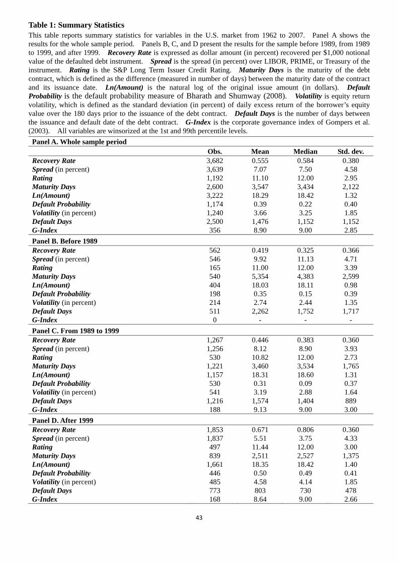
43  

Table 1: Summary Statistics This table reports summary statistics for variables in the U.S. market from 1962 to 2007. Panel A shows the results for the whole sample period. Panels B, C, and D present the results for the sample before 1989, from 1989 to 1999, and after 1999. Recovery Rate is expressed as dollar amount (in percent) recovered per $1,000 notional value of the defaulted debt instrument. Spread is the spread (in percent) over LIBOR, PRIME, or Treasury of the instrument. Rating is the S&P Long Term Issuer Credit Rating. Maturity Days is the maturity of the debt contract, which is defined as the difference (measured in number of days) between the maturity date of the contract and its issuance date. Ln(Amount) is the natural log of the original issue amount (in dollars). Default Probability is the default probability measure of Bharath and Shumway (2008). Volatility is equity return volatility, which is defined as the standard deviation (in percent) of daily excess return of the borrower’s equity value over the 180 days prior to the issuance of the debt contract. Default Days is the number of days between the issuance and default date of the debt contract. G-Index is the corporate governance index of Gompers et al. (2003). All variables are winsorized at the 1st and 99th percentile levels. Panel A. Whole sample period Obs. Mean Median Std. dev. Recovery Rate 3,682 0.555 0.584 0.380 Spread (in percent) 3,639 7.07 7.50 4.58 Rating 1,192 11.10 12.00 2.95 Maturity Days 2,600 3,547 3,434 2,122 Ln(Amount) 3,222 18.29 18.42 1.32 Default Probability 1,174 0.39 0.22 0.40 Volatility (in percent) 1,240 3.66 3.25 1.85 Default Days 2,500 1,476 1,152 1,152 G-Index 356 8.90 9.00 2.85 Panel B. Before 1989 Recovery Rate 562 0.419 0.325 0.366 Spread (in percent) 546 9.92 11.13 4.71 Rating 165 11.00 12.00 3.39 Maturity Days 540 5,354 4,383 2,599 Ln(Amount) 404 18.03 18.11 0.98 Default Probability 198 0.35 0.15 0.39 Volatility (in percent) 214 2.74 2.44 1.35 Default Days 511 2,262 1,752 1,717 G-Index 0 - - - Panel C. From 1989 to 1999 Recovery Rate 1,267 0.446 0.383 0.360 Spread (in percent) 1,256 8.12 8.90 3.93 Rating 530 10.82 12.00 2.73 Maturity Days 1,221 3,460 3,534 1,765 Ln(Amount) 1,157 18.31 18.60 1.31 Default Probability 530 0.31 0.09 0.37 Volatility (in percent) 541 3.19 2.88 1.64 Default Days 1,216 1,574 1,404 889 G-Index 188 9.13 9.00 3.00 Panel D. After 1999 Recovery Rate 1,853 0.671 0.806 0.360 Spread (in percent) 1,837 5.51 3.75 4.33 Rating 497 11.44 12.00 3.00 Maturity Days 839 2,511 2,527 1,375 Ln(Amount) 1,661 18.35 18.42 1.40 Default Probability 446 0.50 0.49 0.41 Volatility (in percent) 485 4.58 4.14 1.85 Default Days 773 803 730 478 G-Index 168 8.64 9.00 2.66

44  

Table 2: Univariate and multivariate regressions of spread and recovery rate

0 1 .Spread RecoveryRate 0 1 2 3 4 5 6 7 8( ) .Spread RecoveryRate Rating MaturityDays SICcode Ln Amount DefaultProbability Volatility DefaultDays

This table presents results of the OLS regressions. Results are shown separately for univariate and multivariate regressions in Panels A and B. The SIC code variable is the control variable for industry effect and it is the 4-digit SIC code. Robust standard errors are in parentheses. Significant levels are indicated by ***, **, and * for 1%, 5%, and 10%, respectively. Panel A. Univariate regression (i) (ii) (iii) (iv) Whole sample period Before 1989 From 1989 to 1999 After 1999 Recovery Rate -4.673*** -1.391** -3.602*** -4.463*** (-26.002) (-2.459) (-12.222) (-16.416) Constant 9.660*** 10.498*** 9.725*** 8.497*** (77.799) (34.576) (59.458) (38.771) Observations 3639 546 1256 1837 R-squared 0.150 0.012 0.108 0.139

Panel B. Multivariate regression (i) (ii) (iii) (iv) Whole sample period Before 1989 From 1989 to 1999 After 1999 Recovery Rate -3.233*** -1.461 -3.081*** -3.933*** (-8.815) (-0.597) (-5.566) (-7.869) Rating 0.292*** 0.455** 0.302*** 0.238*** (5.668) (2.434) (3.704) (3.174) Maturity Days * 10-3 0.288*** -0.373 0.286*** 0.336** (4.716) (-1.140) (4.540) (2.501) SIC code * 10-4 0.633 -0.441 -1.583* 4.243*** (0.886) (-0.098) (-1.725) (3.483) Ln(Amount) 0.076 1.699 -0.151 -0.021 (0.633) (1.423) (-0.813) (-0.117) Default Probability 1.310*** 0.903 1.062* 1.581*** (3.602) (0.695) (1.713) (3.369) Volatility 0.074 -0.321 0.260 0.067 (0.740) (-0.791) (1.400) (0.499) Default Days * 10-3 0.627*** -0.197 0.751*** 1.606*** (4.085) (-0.546) (4.074) (4.305) Constant 2.216 -21.986 6.438* 2.442 (0.924) (-0.927) (1.934) (0.650) Observations 629 44 285 300 R-squared 0.230 0.310 0.240 0.315

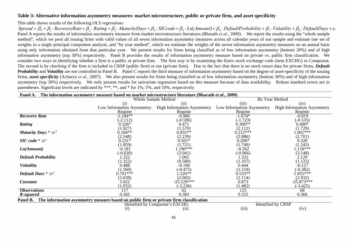
45  

Table 3: Alternative information asymmetry measures: market microstructure, public or private firm, and asset specificity

This table shows results of the following OLS regressions:

0 1 2 3 4 5 6 7 8( ) .Spread RecoveryRate Rating MaturityDays SICcode Ln Amount DefaultProbability Volatility DefaultDays Panel A reports the results of information asymmetry measure from market microstructure literatures (Bharath et al., 2009). We report the results using the “whole sample method”, which we pool all issuing firms with valid values of all seven information asymmetry measures across all calendar years of our sample and estimate one set of weights in a single principal component analysis, and “by year method”, which we estimate the weights of the seven information asymmetry measures on an annual basis using only information obtained from that particular year. We present results for firms being classified as of low information asymmetry (bottom 30%) and of high information asymmetry (top 30%) respectively. Panel B provides the results of information asymmetry measure based on private vs. public firm classification. We consider two ways in identifying whether a firm is a public or private firm. The first way is by examining the firm's stock exchange code (item EXCHG) in Compustat. The second is by checking if the firm is included in CRSP (public firm) or not (private firm). Due to the fact that there is no stock return data for private firms, Default Probability and Volatility are not controlled in Panel B. Panel C reports the third measure of information asymmetry based on the degree of asset-specificity of the issuing firms, asset specificity (Acharya et al., 2007). We also present results for firms being classified as of low information asymmetry (bottom 30%) and of high information asymmetry (top 30%) respectively. We only present results for univariate regression based on this measure because of data availability. Robust standard errors are in parentheses. Significant levels are indicated by ***, **, and * for 1%, 5%, and 10%, respectively. Panel A. The information asymmetry measure based on market microstructure literature (Bharath et al., 2009) Whole Sample Method By Year Method (i) (ii) (iii) (iv) Low Information Asymmetry

RegimeHigh Information Asymmetry

Regime Low Information Asymmetry

RegimeHigh Information Asymmetry

Regime Recovery Rate -2.184** -0.966 -1.674* -0.819 (-2.112) (-0.596) (-1.723) (-0.535) Rating 0.326* 0.471 0.306** 0.490* (1.927) (1.570) (2.112) (1.729) Maturity Days * 10-3 0.184** 0.855** 0.212*** 1.001*** (2.548) (2.239) (2.886) (2.701) SIC code * 10-3 0.231* 0.501* 0.200* 0.328 (1.859) (1.721) (1.749) (1.243) Ln(Amount) -0.181 1.190*** -0.262 1.118*** (-0.630) (3.041) (-0.966) (3.148) Default Probability 1.322 1.065 1.333 2.129 (1.322) (0.580) (1.357) (1.125) Volatility 0.488 -0.196 0.444 -0.127 (1.560) (-0.475) (1.519) (-0.382) Default Days * 10-3 0.701*** 1.526** 0.533** 1.955*** (3.038) (2.065) (2.114) (2.932) Constant 5.022 -25.529*** 6.873 -25.873*** (1.052) (-3.236) (1.482) (-3.425) Observations 117 62 125 68 R-squared 0.365 0.383 0.325 0.366

Panel B. The information asymmetry measure based on public firm or private firm classification Identified by Compustat’s EXCHG Identified by CRSP (i) (ii) (iii) (iv)

46  

Public Firm Private Firm Public Firm Private Firm Recovery Rate -3.337*** -0.462 -3.167*** -2.534** (-10.464) (-0.241) (-10.073) (-2.520) Rating 0.274*** 0.058 0.291*** 0.272*** (7.276) (0.252) (7.313) (2.628) Maturity Days * 10-3 0.253*** 1.281** 0.317*** 1.151*** (4.673) (2.600) (5.597) (3.989) SIC code * 10-3 -0.022 -0.649** -0.019 -0.008 (-0.347) (-2.298) (-0.301) (-0.037) Ln(Amount) -0.096 0.083 -0.082 -0.447 (-0.982) (0.136) (-0.850) (-1.234) Default Days * 10-3 0.296** -0.626 0.328*** 0.178 (2.423) (-0.911) (2.736) (0.402) Constant 7.732*** 5.942 6.830*** 11.983* (3.922) (0.447) (3.448) (1.680) Observations 903 77 1007 188 R-squared 0.185 0.180 0.178 0.252

Panel C. The information asymmetry measure based on asset specificity (Acharya et al., 2007) (i) (ii) Low Information Asymmetry Regime High Information Asymmetry Regime Recovery Rate -3.812*** -0.103 (-3.029) (-0.065)Constant 11.802*** 9.489*** (21.855) (12.285)Observations 91 93R-squared 0.117 0.000

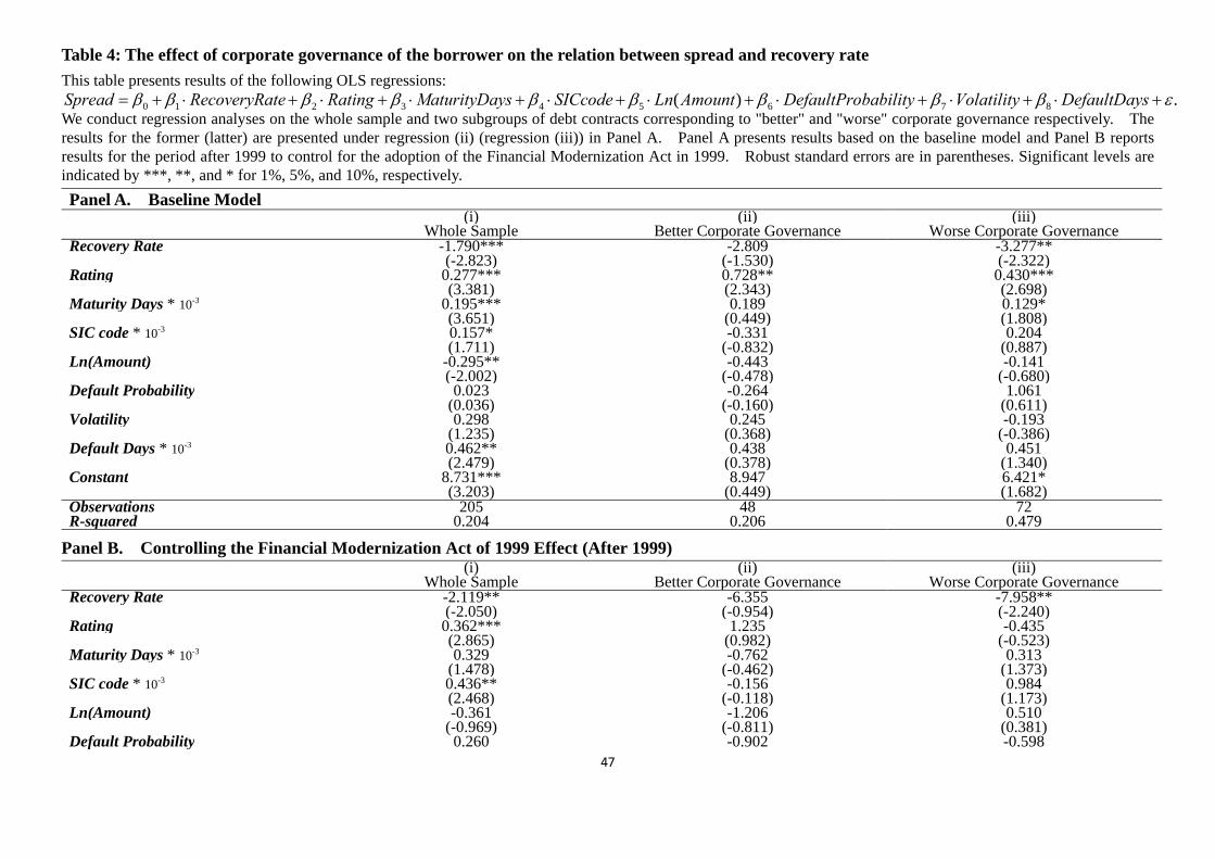
47  

Table 4: The effect of corporate governance of the borrower on the relation between spread and recovery rate

This table presents results of the following OLS regressions:

0 1 2 3 4 5 6 7 8( ) .Spread RecoveryRate Rating MaturityDays SICcode Ln Amount DefaultProbability Volatility DefaultDays We conduct regression analyses on the whole sample and two subgroups of debt contracts corresponding to "better" and "worse" corporate governance respectively. The results for the former (latter) are presented under regression (ii) (regression (iii)) in Panel A. Panel A presents results based on the baseline model and Panel B reports results for the period after 1999 to control for the adoption of the Financial Modernization Act in 1999. Robust standard errors are in parentheses. Significant levels are indicated by ***, **, and * for 1%, 5%, and 10%, respectively. Panel A. Baseline Model (i) (ii) (iii) Whole Sample Better Corporate Governance Worse Corporate Governance Recovery Rate -1.790*** -2.809 -3.277** (-2.823) (-1.530) (-2.322)Rating 0.277*** 0.728** 0.430*** (3.381) (2.343) (2.698)Maturity Days * 10-3 0.195*** 0.189 0.129* (3.651) (0.449) (1.808)SIC code * 10-3 0.157* -0.331 0.204 (1.711) (-0.832) (0.887)Ln(Amount) -0.295** -0.443 -0.141 (-2.002) (-0.478) (-0.680)Default Probability 0.023 -0.264 1.061 (0.036) (-0.160) (0.611)Volatility 0.298 0.245 -0.193 (1.235) (0.368) (-0.386)Default Days * 10-3 0.462** 0.438 0.451 (2.479) (0.378) (1.340)Constant 8.731*** 8.947 6.421* (3.203) (0.449) (1.682)Observations 205 48 72R-squared 0.204 0.206 0.479

Panel B. Controlling the Financial Modernization Act of 1999 Effect (After 1999) (i) (ii) (iii) Whole Sample Better Corporate Governance Worse Corporate Governance Recovery Rate -2.119** -6.355 -7.958** (-2.050) (-0.954) (-2.240)Rating 0.362*** 1.235 -0.435 (2.865) (0.982) (-0.523)Maturity Days * 10-3 0.329 -0.762 0.313 (1.478) (-0.462) (1.373)SIC code * 10-3 0.436** -0.156 0.984 (2.468) (-0.118) (1.173)Ln(Amount) -0.361 -1.206 0.510 (-0.969) (-0.811) (0.381)Default Probability 0.260 -0.902 -0.598

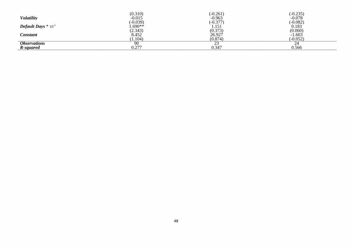
48  

(0.310) (-0.261) (-0.235)Volatility -0.015 -0.963 -0.078 (-0.039) (-0.377) (-0.082)Default Days * 10-3 1.690** 1.151 0.183 (2.343) (0.373) (0.060)Constant 8.452 26.927 -1.603 (1.104) (0.874) (-0.052)Observations 90 23 24R-squared 0.277 0.347 0.566

49  

Table 5: The effect of credit rating of the borrower on the relation between spread and recovery rate

0 1 2 3 4 5 6 7 8( ) .Spread RecoveryRate Rating MaturityDays SICcode Ln Amount DefaultProbability Volatility DefaultDays This table examines the explanatory power of recovery rate in contingent on the fact that the issuer belongs to investment grade verse non-investment grade at the issuance of the debt contract. We conduct regression analyses for the whole sample and three subsample periods corresponding to "Before 1989", "From 1989 to 1999" and "After 1999" period, respectively. The whole sample and three subsamples are divided into two subgroups: investment grade (denoted as Invest. Grade) and non-investment grade (denoted as Non-Invest. Grade). The S&P’s ratings of the former group are BBB- or higher; whereas BB+ or lower for the latter. Robust standard errors are in parentheses. Significant levels are indicated by ***, **, and * for 1%, 5%, and 10%, respectively. Whole Sample Period Before 1989 From 1989 to 1999 After 1999 (i) (ii) (iii) (iv) (v) (vi) (vii) (viii) Invest. Grade Non-Invest.

Grade Invest. Grade Non-Invest.

Grade Invest. Grade Non-Invest.

Grade Invest. Grade Non-Invest.

Grade Recovery Rate -1.659** -3.728*** 0.515 -3.065 -1.705* -3.471*** -4.063*** -4.396*** (-2.065) (-8.672) (0.019) (-0.700) (-1.909) (-4.788) (-2.683) (-7.429) Rating 0.419*** 0.421*** -0.605 0.782 0.464*** 0.491** -0.002 0.364** (3.233) (3.685) (-0.036) (1.170) (4.086) (2.022) (-0.006) (2.577) Maturity Days * 10-3 0.232*** 0.444*** -0.270 -0.331 0.190*** 0.763** 0.349** 0.240 (4.653) (2.954) (-0.050) (-0.677) (3.687) (2.100) (2.210) (0.936) SIC code * 10-3 0.388*** -0.158 -0.501 -0.110 0.171 -0.291** 0.869*** 0.143 (3.725) (-1.614) (-0.039) (-0.160) (1.554) (-2.265) (4.836) (0.806) Ln(Amount) -0.302** 0.273 -6.382 1.943* -0.333** 0.205 0.142 0.023 (-2.550) (1.499) (-0.107) (1.787) (-2.569) (0.550) (0.433) (0.104) Default Probability 2.605*** 1.238*** 5.658 0.656 5.141 0.918 0.680 1.398** (2.898) (3.074) (0.156) (0.326) (1.406) (1.412) (0.677) (2.526) Volatility -0.464 0.117 2.640 -0.315 -0.740 0.325* 0.337 -0.017 (-1.483) (1.104) (0.031) (-0.593) (-1.066) (1.671) (0.695) (-0.126) Default Days * 10-3 0.302 0.875*** -0.661 0.770 0.740*** 0.758** 4.069*** 1.490*** (1.635) (4.075) (-0.072) (0.472) (3.096) (2.483) (4.414) (3.148) Constant 8.236*** -2.680 129.393 -31.087 8.957*** -3.437 -2.995 2.447 (3.271) (-0.652) (0.118) (-1.331) (3.547) (-0.405) (-0.427) (0.514) Observations 163 466 11 33 91 194 61 239 R-squared 0.388 0.233 0.858 0.289 0.509 0.289 0.561 0.256

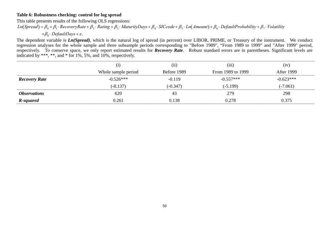
50  

Table 6: Robustness checking: control for log spread This table presents results of the following OLS regressions:

0 1 2 3 4 5 6 7

8

( ) ( )

.

Ln Spread RecoveryRate Rating MaturityDays SICcode Ln Amount DefaultProbability Volatility

DefaultDays

The dependent variable is Ln(Spread), which is the natural log of spread (in percent) over LIBOR, PRIME, or Treasury of the instrument. We conduct regression analyses for the whole sample and three subsample periods corresponding to "Before 1989", “From 1989 to 1999” and "After 1999" period, respectively. To conserve space, we only report estimated results for Recovery Rate. Robust standard errors are in parentheses. Significant levels are indicated by ***, **, and * for 1%, 5%, and 10%, respectively. (i) (ii) (iii) (iv)

Whole sample period Before 1989 From 1989 to 1999 After 1999

Recovery Rate -0.526*** -0.119 -0.557*** -0.623***

(-8.137) (-0.347) (-5.199) (-7.061)

Observations 620 43 279 298

R-squared 0.261 0.138 0.278 0.375

51  

Table 7: Robustness checking: endogeneity

This table reports results of the two-stage least square regression:

0 1 2 3 4 5 6 7

8 9

( )

.

RecoveryRate Rating MaturityDays SICcode Ln Amount DefaultProbability Volatility DefaultDays

BankruptcyCourt GDPGrowthRate

0 1 2 3 4 5 6 7

8

( ) ( )

.

Spread Fitted RecoveryRate Rating MaturityDays SICcode Ln Amount DefaultProbability Volatility

DefaultDays

The endogenous variable is Recovery Rate. Two instruments are used in the analysis: bankruptcy court district dummy (Bankruptcy Court), and the preceding 12-monthes moving average U.S. GDP growth rate (GDP Growth Rate). To conserve space, we only report results of the two instrumental variables in the first stage regression and the Fitted Recovery Rate in the second stage regression. Robust standard errors are in parentheses. Significant levels are indicated by ***, **, and * for 1%, 5%, and 10%, respectively. Panel A: Two-stage least square regression results Whole sample period Before 1989 From 1989 to 1999 After 1999 (i) (ii) (iii) (iv) (v) (vi) (vii) (viii) First/Second Stage: First Second First Second First Second First Second Fitted Recovery Rate -3.516** 0.768 1.363 -5.630*** (-1.979) (0.122) (0.369) (-2.858) Bankruptcy Court * 10-3 2.263*** -0.032 1.291 1.763 (3.359) (-0.015) (1.276) (1.629) GDP Growth Rate 3.607*** -4.454 2.711*** 5.059*** (5.178) (-1.298) (2.919) (3.579) Observations 588 588 38 38 272 272 278 278 R-squared 0.121 0.267 0.150 0.227 0.081 0.053 0.178 0.329 Panel B: Testing for Instrument Relevance:

- Staiger and Stock (1997) F-Statistic: 18.7454 F-Statistic: 0.8445 F-Statistic: 4.8178 F-Statistic: 8.5644 P-value: < 0.0001 P-value: 0.4404 P-value: 0.0088 P-value: 0.0002

- Bound, Jaeger, and Baker (1995) Partial R2: 0.0414 Partial R2: 0.0560 Partial R2: 0.0205 Partial R2: 0.0534

- Shea (1997) Partial R2: 0.0449 Partial R2: 0.0618 Partial R2: 0.0218 Partial R2: 0.0610 Panel C: Testing for Instrument Exogeneity (Exclusion Restriction):

- Tests of over-identifying restrictions (Ho: instruments are exogenous): Sargan (1958) Chi-Squared: < 0.0001 Chi-Squared: 0.0939 Chi-Squared: 0.9271 Chi-Squared: 0.4730 P-value: 0.9950 P-value: 0.7592 P-value: 0.3356 P-value: 0.4916

- Tests of over-identifying restrictions (Ho: instruments are exogenous): Basmann (1960) Chi-Squared: < 0.0001 Chi-Squared: 0.0694 Chi-Squared: 0.8961 Chi-Squared: 0.4568 P-value: 0.9950 P-value: 0.7922 P-value: 0.3438 P-value: 0.4991

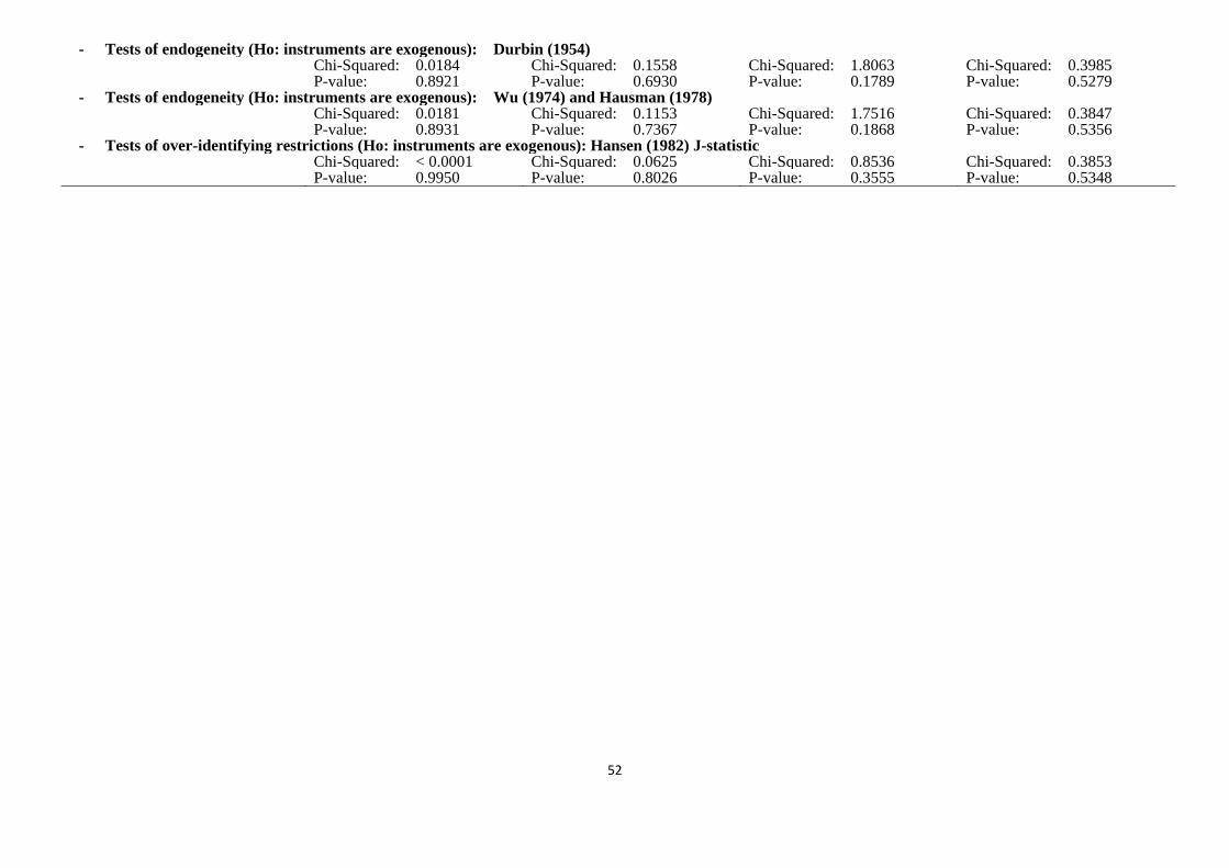
52  

- Tests of endogeneity (Ho: instruments are exogenous): Durbin (1954) Chi-Squared: 0.0184 Chi-Squared: 0.1558 Chi-Squared: 1.8063 Chi-Squared: 0.3985 P-value: 0.8921 P-value: 0.6930 P-value: 0.1789 P-value: 0.5279

- Tests of endogeneity (Ho: instruments are exogenous): Wu (1974) and Hausman (1978) Chi-Squared: 0.0181 Chi-Squared: 0.1153 Chi-Squared: 1.7516 Chi-Squared: 0.3847 P-value: 0.8931 P-value: 0.7367 P-value: 0.1868 P-value: 0.5356

- Tests of over-identifying restrictions (Ho: instruments are exogenous): Hansen (1982) J-statistic Chi-Squared: < 0.0001 Chi-Squared: 0.0625 Chi-Squared: 0.8536 Chi-Squared: 0.3853 P-value: 0.9950 P-value: 0.8026 P-value: 0.3555 P-value: 0.5348

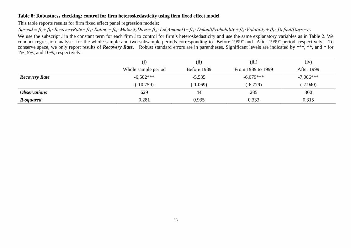
53  

Table 8: Robustness checking: control for firm heteroskedasticity using firm fixed effect model

This table reports results for firm fixed effect panel regression models:

1 2 3 4 5 6 7( ) .iSpread RecoveryRate Rating MaturityDays Ln Amount DefaultProbability Volatility DefaultDays We use the subscript i in the constant term for each firm i to control for firm’s heteroskedasticity and use the same explanatory variables as in Table 2. We conduct regression analyses for the whole sample and two subsample periods corresponding to "Before 1999" and "After 1999" period, respectively. To conserve space, we only report results of Recovery Rate. Robust standard errors are in parentheses. Significant levels are indicated by ***, **, and * for 1%, 5%, and 10%, respectively. (i) (ii) (iii) (iv)

Whole sample period Before 1989 From 1989 to 1999 After 1999

Recovery Rate -6.502*** -5.535 -6.079*** -7.006***

(-10.759) (-1.069) (-6.779) (-7.940)

Observations 629 44 285 300

R-squared 0.281 0.935 0.333 0.315

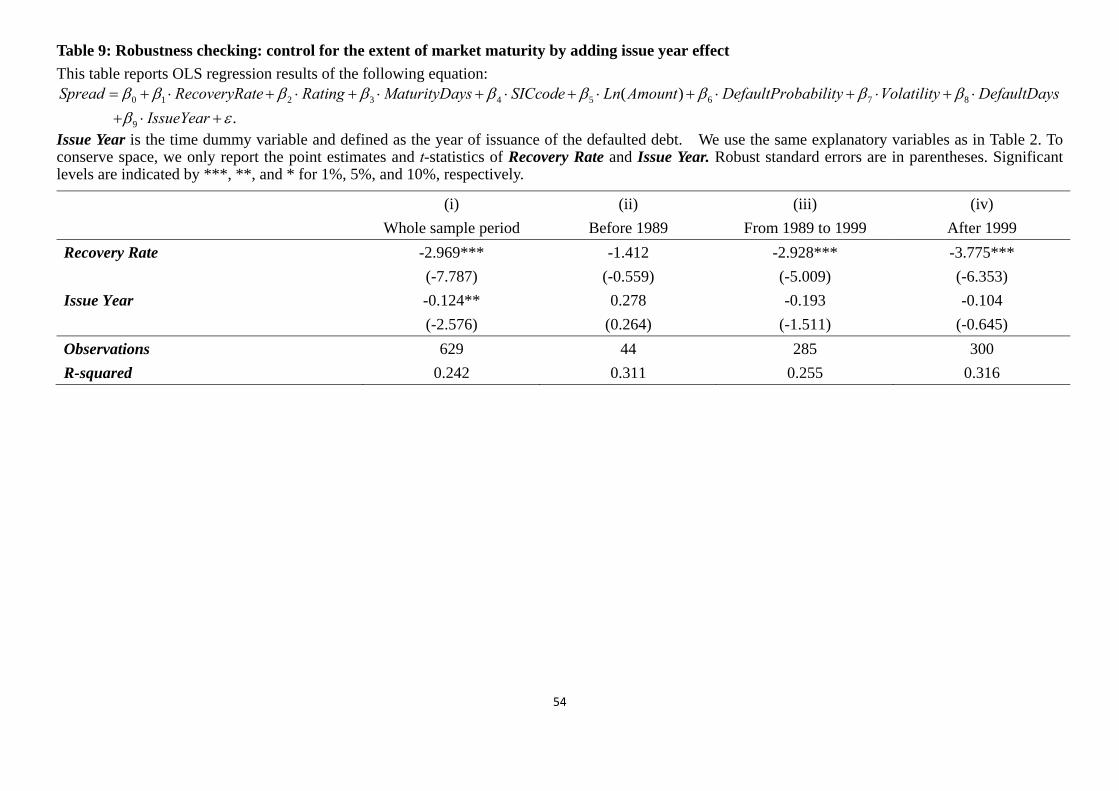
54  

Table 9: Robustness checking: control for the extent of market maturity by adding issue year effect

This table reports OLS regression results of the following equation:

0 1 2 3 4 5 6 7 8

9

( )

.

Spread RecoveryRate Rating MaturityDays SICcode Ln Amount DefaultProbability Volatility DefaultDays

IssueYear

Issue Year is the time dummy variable and defined as the year of issuance of the defaulted debt. We use the same explanatory variables as in Table 2. To conserve space, we only report the point estimates and t-statistics of Recovery Rate and Issue Year. Robust standard errors are in parentheses. Significant levels are indicated by ***, **, and * for 1%, 5%, and 10%, respectively. (i) (ii) (iii) (iv)

Whole sample period Before 1989 From 1989 to 1999 After 1999

Recovery Rate -2.969*** -1.412 -2.928*** -3.775***

(-7.787) (-0.559) (-5.009) (-6.353)

Issue Year -0.124** 0.278 -0.193 -0.104

(-2.576) (0.264) (-1.511) (-0.645)

Observations 629 44 285 300

R-squared 0.242 0.311 0.255 0.316

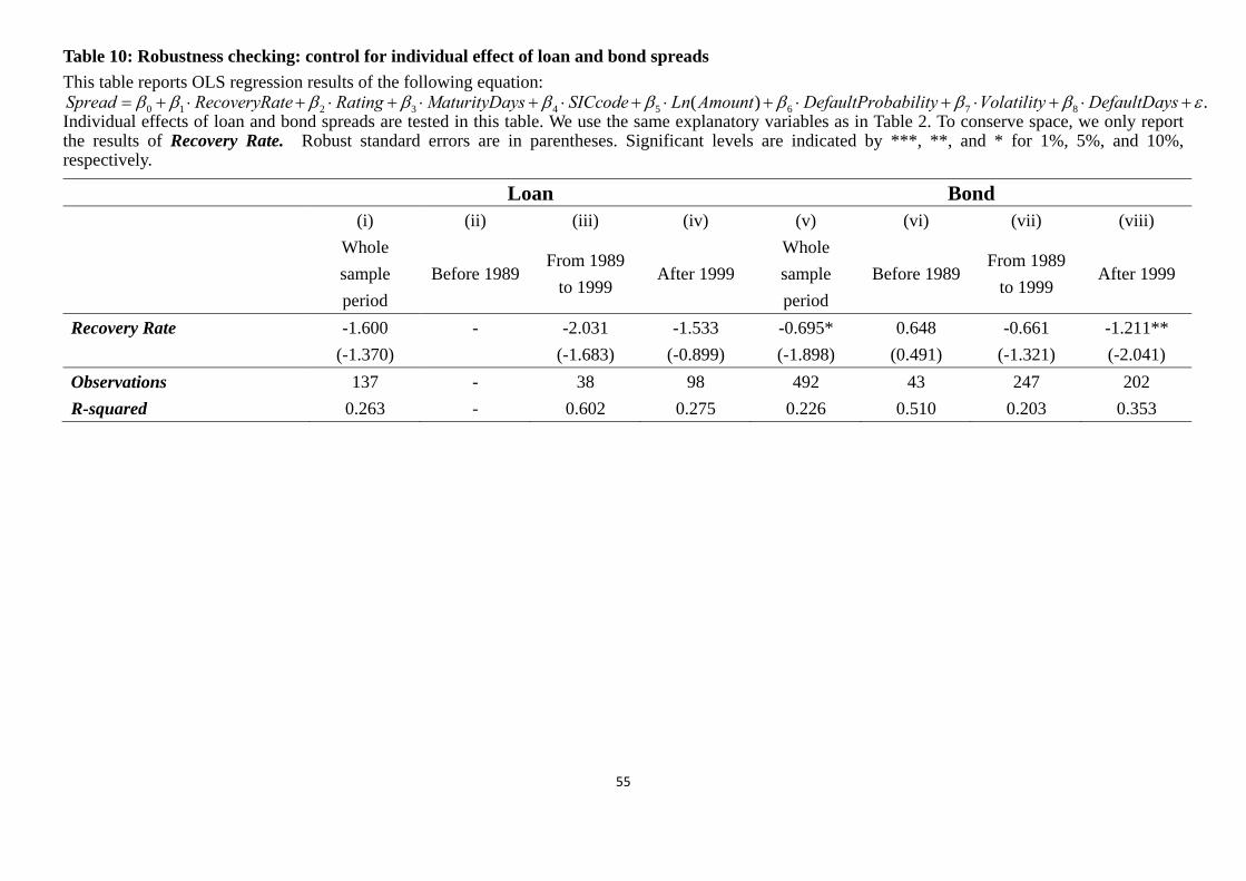
55  

Table 10: Robustness checking: control for individual effect of loan and bond spreads

This table reports OLS regression results of the following equation:

0 1 2 3 4 5 6 7 8( ) .Spread RecoveryRate Rating MaturityDays SICcode Ln Amount DefaultProbability Volatility DefaultDays Individual effects of loan and bond spreads are tested in this table. We use the same explanatory variables as in Table 2. To conserve space, we only report the results of Recovery Rate. Robust standard errors are in parentheses. Significant levels are indicated by ***, **, and * for 1%, 5%, and 10%, respectively. Loan Bond (i) (ii) (iii) (iv) (v) (vi) (vii) (viii)

Whole

sample

period

Before 1989From 1989

to 1999 After 1999

Whole

sample

period

Before 1989From 1989

to 1999 After 1999

Recovery Rate -1.600 - -2.031 -1.533 -0.695* 0.648 -0.661 -1.211**

(-1.370) (-1.683) (-0.899) (-1.898) (0.491) (-1.321) (-2.041)

Observations 137 - 38 98 492 43 247 202

R-squared 0.263 - 0.602 0.275 0.226 0.510 0.203 0.353

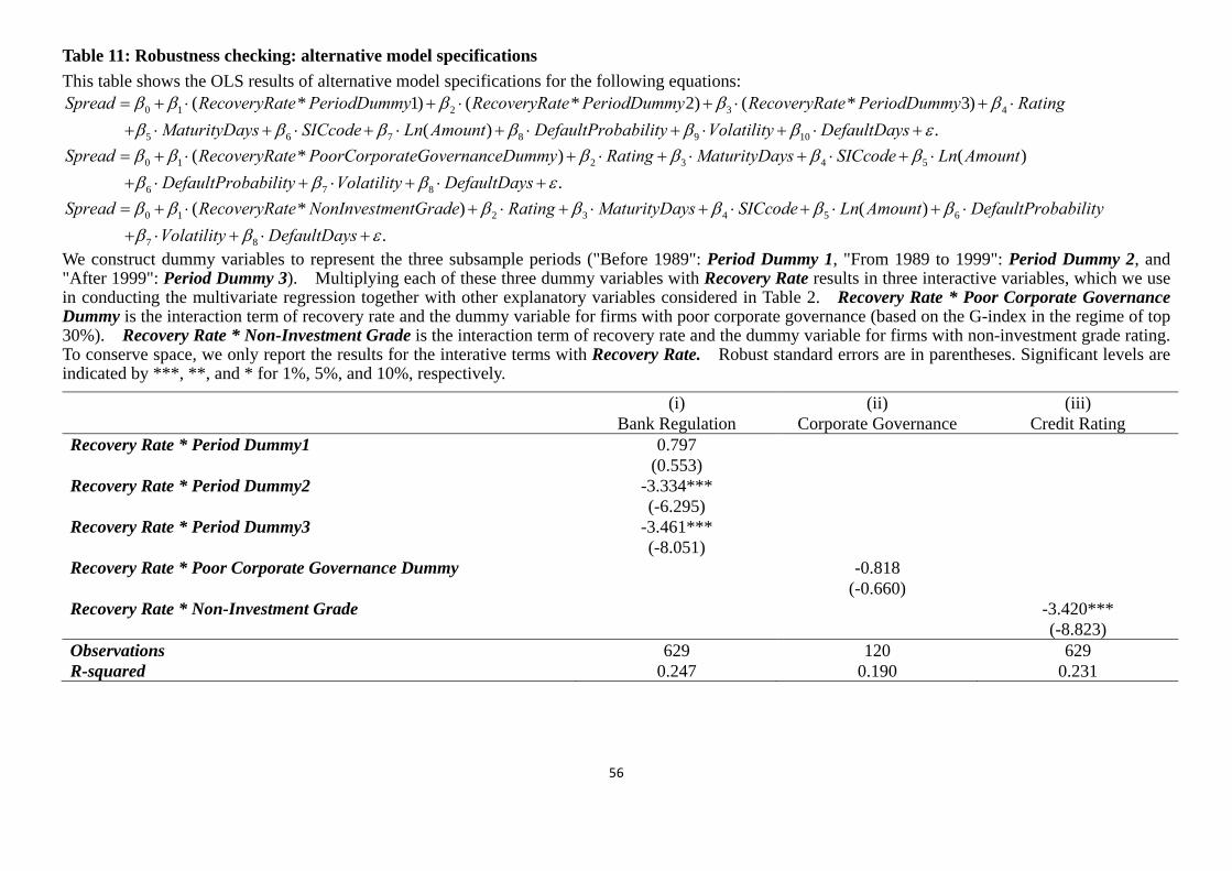
56  

Table 11: Robustness checking: alternative model specifications

This table shows the OLS results of alternative model specifications for the following equations:

0 1 2 3 4

5 6 7 8 9 10

( * 1) ( * 2) ( * 3)

( )

Spread RecoveryRate PeriodDummy RecoveryRate PeriodDummy RecoveryRate PeriodDummy Rating

MaturityDays SICcode Ln Amount DefaultProbability Volatility Defaul

.tDays

0 1 2 3 4 5

6 7 8

( * ) ( )

.

Spread RecoveryRate PoorCorporateGovernanceDummy Rating MaturityDays SICcode Ln Amount

DefaultProbability Volatility DefaultDays

0 1 2 3 4 5 6

7 8

( * ) ( )

.

Spread RecoveryRate NonInvestmentGrade Rating MaturityDays SICcode Ln Amount DefaultProbability

Volatility DefaultDays

We construct dummy variables to represent the three subsample periods ("Before 1989": Period Dummy 1, "From 1989 to 1999": Period Dummy 2, and "After 1999": Period Dummy 3). Multiplying each of these three dummy variables with Recovery Rate results in three interactive variables, which we use in conducting the multivariate regression together with other explanatory variables considered in Table 2. Recovery Rate * Poor Corporate Governance Dummy is the interaction term of recovery rate and the dummy variable for firms with poor corporate governance (based on the G-index in the regime of top 30%). Recovery Rate * Non-Investment Grade is the interaction term of recovery rate and the dummy variable for firms with non-investment grade rating. To conserve space, we only report the results for the interative terms with Recovery Rate. Robust standard errors are in parentheses. Significant levels are indicated by ***, **, and * for 1%, 5%, and 10%, respectively. (i) (ii) (iii) Bank Regulation Corporate Governance Credit Rating Recovery Rate * Period Dummy1 0.797 (0.553) Recovery Rate * Period Dummy2 -3.334*** (-6.295) Recovery Rate * Period Dummy3 -3.461*** (-8.051) Recovery Rate * Poor Corporate Governance Dummy -0.818 (-0.660) Recovery Rate * Non-Investment Grade -3.420*** (-8.823) Observations 629 120 629 R-squared 0.247 0.190 0.231

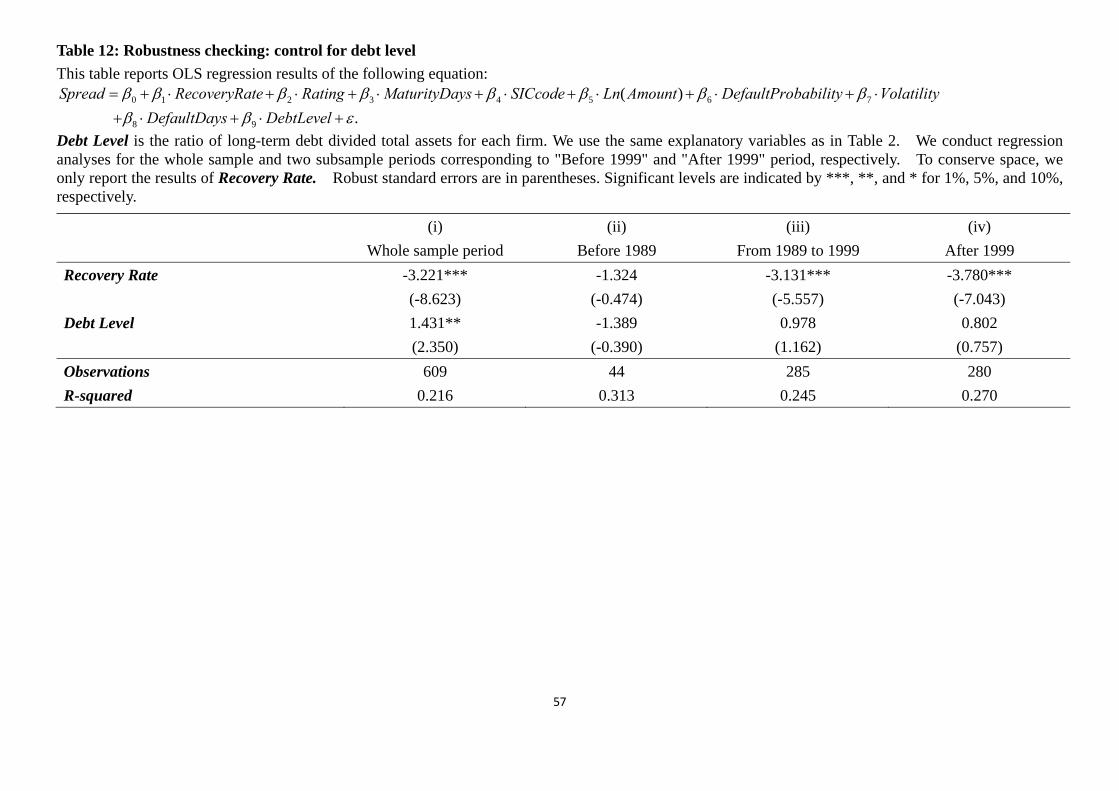
57  

Table 12: Robustness checking: control for debt level

This table reports OLS regression results of the following equation:

0 1 2 3 4 5 6 7

8 9

( )

.

Spread RecoveryRate Rating MaturityDays SICcode Ln Amount DefaultProbability Volatility

DefaultDays DebtLevel

Debt Level is the ratio of long-term debt divided total assets for each firm. We use the same explanatory variables as in Table 2. We conduct regression analyses for the whole sample and two subsample periods corresponding to "Before 1999" and "After 1999" period, respectively. To conserve space, we only report the results of Recovery Rate. Robust standard errors are in parentheses. Significant levels are indicated by ***, **, and * for 1%, 5%, and 10%, respectively. (i) (ii) (iii) (iv)

Whole sample period Before 1989 From 1989 to 1999 After 1999

Recovery Rate -3.221*** -1.324 -3.131*** -3.780***

(-8.623) (-0.474) (-5.557) (-7.043)

Debt Level 1.431** -1.389 0.978 0.802

(2.350) (-0.390) (1.162) (0.757)

Observations 609 44 285 280

R-squared 0.216 0.313 0.245 0.270