institute for economic studies, keio university keio-ies discussion paper · pdf...

Institute for Economic Studies, Keio University

Keio-IES Discussion Paper Series

誰と比較するか？参照グループの決定要因に関する研究

周梦媛

2018年 1 月 10 日

DP2018-001

https://ies.keio.ac.jp/publications/8840/

Institute for Economic Studies, Keio University

2-15-45 Mita, Minato-ku, Tokyo 108-8345, Japan

[email protected]

10 January, 2018

誰と比較するか？参照グループの決定要因に関する研究

周梦媛

IES Keio DP2018-001

2018 年 1月 10日

JEL Classification: C25; D00; J31

キーワード: 参照グループ; 相対的な生活水準; routine standards

【要旨】

本研究の目的は、日米において、生活水準の参照グループが誰なのか、またそれがどのように

して決定されるのかを明らかにすることである。分析の結果、マクロや金融の文献でしばしば

仮定されている国の平均的な人や、収入の比較対象である同僚や友人と異なり、大部分の日本

人とアメリカ人は隣人を比較対象としていることが示された。この分析結果は、相対的な生活

水準の参照グループを選択する際に、「Routine Standards」を使用する可能性を示唆している。

また、本研究では、参照グループ自体が生活水準に与える影響を検証した。その結果、隣人と

比較する人は、ほかの参照グループを選択する人よりも、相対的な生活水準を高く知覚するこ

とを確認した。

周梦媛

慶應義塾大学大学院経済学研究科

〒108-8345

東京都港区三田2-14-45

[email protected]

謝辞：本論文の発行に際して、大垣昌夫先生よりご推薦頂いた。ここに感謝の意を記した

い。

1

Who are the Joneses that You are Keeping up with?

A Study about how Reference Groups are Determined1

Mengyuan Zhou2

Graduate School of Economics, Keio University

Abstract

This study empirically investigates who is chosen as the reference group in the standard of

living comparison and how it is chosen in Japan and the United States. The results show that

majority people will compare to their neighbor instead of the average people in the nation (which

is often assumed in the macro and finance literature), colleagues or friends (reference groups in

income comparison) in both countries. This paper suggests that people may use the routine

standards when facing the selection of reference groups in relative standard of living. In addition,

this paper tests the influence of reference group itself on the standard of living. The result unveils

that those who compare to their neighbor will rate the relative standard of living higher than the

others.

Keywords: reference groups, relative standard of living, routine standards

JEL classification: C25, D00, J31

1 I am grateful to Masao Ogaki, Colin R Mckenzie, Fumio Ohtake, and participants of the 10th Annual Conference

of the Association of Behavioral Economics and Finance. This research uses micro data from the Preference Parameters

Study of Osaka University’s 21st Century COE Program ‘Behavioral Macrodynamics Based on Surveys and

Experiments’ and its Global COE project ‘Human Behavior and Socioeconomic Dynamics’. I acknowledge the

program/project’s contributors: Yoshiro Tsutsui, Fumio Ohtake, and Shinsuke Ikeda. This work was supported by

Doctorate Student Grant-in-Aid Program from Keio University. 2 Corresponding author.

E-mail address: [email protected]

mailto:[email protected]

2

1. Introduction

People are inevitable to compare with others for the purpose of measuring their opinions and

abilities (Festinger, 1954). Especially when objective measurement doesn’t work, reference

groups will be used for self-evaluation, self-enhancement, and self-improvement (Guimond,

2006).

Fehr and Schmidt’s theoretical model (1999) presumes that people’s behavior and subjective

well-being are affected by relative payoffs. And the importance of relative payoffs associated

with subjective well-being has been observed in many empirical researches (Clark and Oswald,

1996; Clark et al., 2009; Clark and Senik, 2010; Clark et al., 2013; Ferrer-i-Carbonell, 2005;

Knight et al., 2009; Mayraz et al., 2009; McBride, 2001; Yamada and Sato, 2013).

What kind of relative indicators has been used in Economics? In general, there are three ways

to define the relative indicators in previous literature which are macroeconomic indicators (Abel,

1990; Campbell and Cochrane, 1999; Duesenberry, 1949; Di Tella et al., 2003; Easterlin, 1974;

Easterlin, 1995; Easterlin et al., 2010; Gali, 1994), the indicators generated from those who are in

the similar socio-economic groups (Clark et al., 1996; Clark et al., 2009; Ferrer-i-Carbonell, 2005;

McBride, 2001; Pérez-Asenjo, 2011), and the indicators generated from self-reported reference

groups (Clark and Senik, 2010; Clark et al., 2013; Knight et al., 2009; Mayraz et al., 2009;

Mangyo and Park 2011; Neumark and Postlewaite, 1998; Yamada and Sato, 2013).

What kind of reference groups has been used in Economics? And which one is more crucial?

Here the author defines two types of reference groups: objective reference groups and subjective

reference groups.3 Objective reference groups are the groups which people compare to with given

socio-economic characteristics, such as similar age, similar educational attainment, same

occupation, in the same organization, etc. Using macroeconomic indicators implicitly assumes

that people are taking the whole nation as the reference group. As a result, the nationwide

comparison is a kind of objective reference groups as well. Subjective reference groups are the

ones which individuals socially interact with indeed.4 The subjective ones mainly refer to self-

reported reference groups in an interview or a survey, such as neighbors, friends, relatives,

classmates, etc. Mangyo and Park (2011) mentioned that the reference groups people social

contact with frequently are more salient, which suggested that subjective reference groups may

be much more essential because these kinds of reference groups are the ones people associate

with.

3 The names of objective and subjective reference groups stemmed from objective and subjective status in

psychology introduced by Hyman (1942). 4 Clark et al. (2009) categorized the reference groups into the one that individuals interact with, and the other which

is similar to them.

3

Why is the study of the reference groups prominent? Firstly, whom do individuals compare to

and how do they compare to such peer group in Economics are still shrouded in mystery. Without

knowing the peer group, how could we define any variables related to the word ‘relative’?

Secondly, what Hyman (1942) found suggested that under disparate dimensions, people would

compare to diverse peer groups, which implies that the reference groups in income comparison

(Clark and Senik, 2010; Clark et al., 2013; Yamada and Sato, 2013) might not be held in standard

of living (SOL) comparison. Additionally, SOL is a much more general and overall evaluation of

living circumstance. Also, the comparison direction, which refers to the reference group itself,

has an impact on happiness (Clark and Senik, 2010).

This is the first study, which will reveal the self-reported reference groups in SOL comparison

in Japan and the United States, and test how people will choose such specific reference groups.

The results show that the most cited reference group is the neighbor. There are 13.9% Japanese

and 16.3% Americans compare to the average people in Japan and the United States. Contrary to

what the previous literature found in income comparison, employees are the second and the fourth

largest reference groups in Japan and the United States, respectively. Therefore, it is inappropriate

and incongruous to use macroeconomics indicators and income’s reference groups as the

reference groups of SOL. Japanese and females are less likely to do nationwide comparison than

Americans and males. The Blinder-Oaxaca decomposition reveals that the significant gap in

country and gender of the mean of those who compare nationwide is mainly explained by the

coefficients instead of the endowments. Then I apply the routine standards to verify the

explanation for the determination of the reference groups. Even from the information accessibility

prospect, the SOL of neighbor is much more effortless to observe than that of other work

colleagues, the evidence indicates that those who are working for a company and full-time

workers are more likely to compare to other workers to neighbors. The routine standards activate

because that full-time employees compare to or be compared to other colleagues more often than

part-time ones. In addition, the result demonstrates that those who compare to neighbor evaluate

their relative standard of living (RSOL) higher than those who compare to classmates, relatives,

mama friends, friends, etc.

This study is organized as follows. Section 2 describes the data I used to present empirical

result. Section 3 describes the direction (compares to whom) and determination (who will or will

not compare to whom) of the reference groups, and interpretation about why people choose their

reference groups. Section 4 shows the impact of reference groups on the relative standard of living.

Section 5 concludes and discusses.

4

2. Data

Preference Parameters Study of Osaka University is used in this research. This panel survey

has been conducted in Japan since 2004, and in the United States since 2005 by the Institution of

Social and Economic Research of Osaka University. They use a random sample drawn from 20-

69 years old in the wave of 2004 in Japan and 18-99 years old in the wave of 2005 in the United

States. The latest fresh samples were selected in 2009 in both two countries.

The 2011 wave data sets of Japan and the US are used in this paper. There are two main

questions in the questionnaire that will be used in the analyses. Taking the Japan 2011 Preference

Parameters Study as an example, question 15 asked ‘How does your standard of living compare

with that of the people around you’, followed by the question ‘In Q.15, with whom did you

compare your standard of living’. The respondents could select one and only one among the

following 13 reference groups listed in the questionnaire. (see Appendix 1)

3. Direction and Determination of Reference Groups

3.1 Who are the Joneses in the standard of living comparison?

Table 1 shows the distribution of the reference groups. Over 35% respondents compare SOL

to neighbors in Japan and the United States. The average person in the nation is the second major

comparison subject in the United States, and the third in Japan. For both males and females in

Japan and the United States, majority compare to their neighbor instead of the average person in

the nation. There are some obvious distinctions in gender for reference groups. More American

and Japanese men compare to classmates and other workers than women, and more American and

Japanese women compare to relatives and friends than men. The extraordinary high percentage

of ‘Mama friend’5 in Japanese female subsample is mainly due to the Mama Caste (Mama Kasuto

in Japanese)6 experienced by mothers whose children are friends or classmates. Statistically,

there is a significant difference in reference groups over gender in Japan and the United States.7

Insert Table 1 Here

5 Here I refer to ‘Families of your children’s classmates’ as ‘Mama friend’ (‘Mama-tomo’ in Japanese). Because

there is an exceptionally high percentage of Japanese females compare to ‘Mama friend’, and there exists a Japanese

word ‘Mama-tomo’ to describe such unique and special type of relationship in Japan. For the most family in Japan,

mothers are responsible for picking up children, and they become ‘mama-tomo’ just because their children are friends

or in the same class. However, Mama friend is not friends. 6 ‘Mama Caste’ refers to a kind of ranking system, which is ranked by household income, children’s learning ability,

husband’s occupation, etc. 7 The surveys for China urban areas, conducted in 6 cities, were not available until 2009. 2012 China survey provides

that only 5.8% Chinese compare with the whole country, and it is insignificant in the distribution of reference groups

over gender.

5

Appendix 1A shows that the most cited reference group is always ‘neighbor’ from 2008 to

2012. Even if individual’s choice varies over years, the distribution’s ranking of reference groups

of the whole sample doesn’t change a lot.

3.2 Who will / will not compare to the whole nation or neighbor

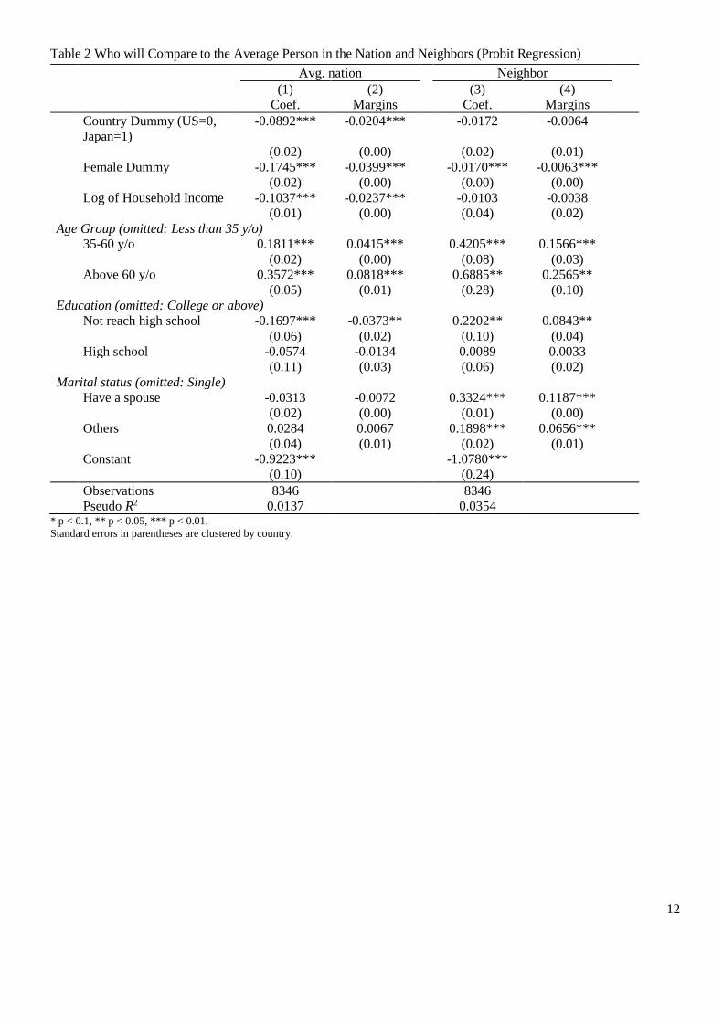
Table 2 presents coefficients and marginal effects of Probit regression by taking those who

choose to compare nationwide or neighbor as ‘1’, and those who choose the other 12 reference

groups as ‘0’.

Insert Table 2 Here

The columns (1) and (2) of Table 2 show that Japanese, females, individuals from rich families

and those who haven’t finish high school are less likely to compare to average person in the nation

than the Americans, males, the poor and those who have graduated from college or above,

respectively. While elderly people are more likely to compare nationwide than those who are less

than 35 years old. The columns (3) and (4) of Table 2 show that those who are younger than 35

years old and the single are less likely to compare to neighbors; on the contrary, males, less

educated people are more likely to compare to neighbors than females and well-educated people.

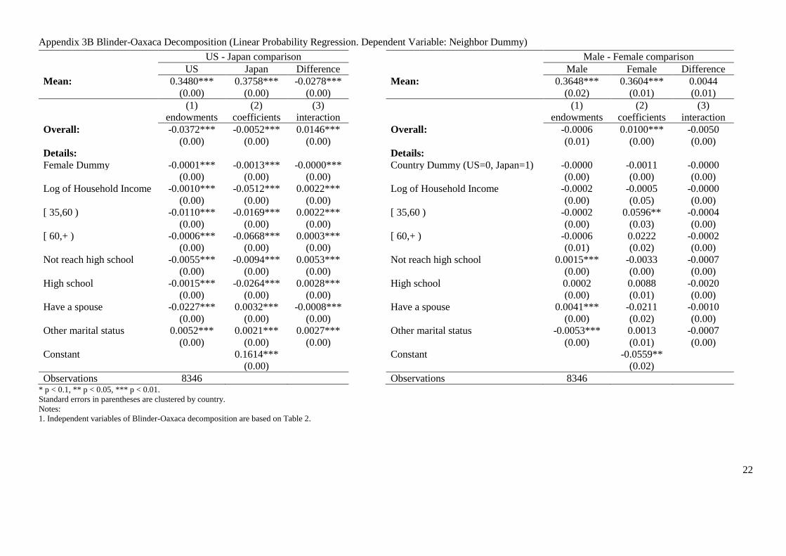
To explore the differences for those who will compare to average people in the nation in detail,

Table 3 provides the T-test result and Blinder-Oaxaca decomposition based on Probit regression

(Appendix 3A and Appendix 3B provide Blinder-Oaxaca decomposition based on linear

probability regression in detail). The mean of those who compare to the average people in the

nation is 0.1616 for the United States and 0.1377 for Japan with a significant gap of 0.0239. The

differences in coefficients account for 104.23% of the gap. Also, the mean of those who compare

to the average people in the nation is 0.1694 for males and 0.1314 for females with a significant

gap of 0.0381. The differences in coefficients account for 100.18% of the gap. Concurrently, the

mean of those who compare to neighbors is 0.3480 and 0.3758 for the United States and Japan,

respectively, with a significant difference of 0.0278 and over 100% of the difference is explained

by the endowments. While there is no significant gap between males and females.

Insert Table 3 Here

Table 4A shows the results of Multinomial Logit regression with all the same independent

variables in Table 2 controlled and the ‘Neighbor’ category omitted. Japanese relative to the

Americans, are more likely to compare to workers to neighbors, but less likely to compare to the

average person in the nation and others to neighbors. Females are less likely than males to

compare to the average person in the nation to neighbors. While Japanese females are less likely

6

to compare to workers than Japanese males, but American females are more likely than American

males. With the age grows, people are more likely to compare to their neighbors. Less educated

people are more likely to compare to neighbors to the average person in Japan and the United

States, which demonstrate the results in Table 2. In general, singles are less likely to compare to

neighbors than married individuals or the ones in any other marital status.

Insert Table 4A Here

Insert Table 4B Here

3.3 How do we choose to whom we compare?

In income comparison, the most cited reference groups are work colleagues in European

countries and friends in Japan (Clark and Senik, 2010; Clark et al., 2013; Yamada and Sato,

2013).8 In previous sections, the results demonstrated that majority Japanese and Americans

choose neighbors as reference groups in SOL comparison instead of colleagues or friends. Why

is the direction of comparison different? As I have mentioned before, one possible explanation is

that the questionnaire is asking about SOL, which is not only focused on income but also implies

about the comparison in consumption, leisure, daily life, etc. Under this different comparison

dimension, people will choose different reference groups which are consistent with Hyman’s

finding. Also from the information accessibility prospect, everyday life has provided much

opportunity to observe neighbor’s SOL than their colleagues or friends.

Then here brings us another question that since it is easier to compare to neighbors than work

colleagues towards SOL, why there is more than 10% of Japanese and Americans choose work

colleagues as the reference groups for SOL comparison? One explanation is the concept of

routines. Betsch et al. (2002) define the routine as:

‘option that comes to mind as a solution when the decision maker recognized a particular

decision problem’

Instead of considering all the possible alternatives, people will pick up the solution which

matches the problem, in terms of the application of the routines as a more efficient way (Betsch

et al. 2002; Guimond, 2006). Mussweiler and Rüter (2003) define the routine standard as a

checkpoint that has been used frequently spontaneously for social comparison and they show the

evidence of the implementation of the routine standard in self-evaluation.

As a result, we compare to or be compared to our work colleagues unintentionally and

frequently in the workplace all the time, then people follow this routine in selecting the reference

8 European Social Survey includes ‘Work colleagues/ Family members/ Friends/ Others/ Don’t compare/ Not

applicable/ Don’t know’. Internet-based survey conducted in Japan by Nikkei includes ‘family/ neighbors/ friends/

colleagues/ do not care/ others’

7

group of SOL. Consequently, I assume that those who are working for a company or full-time

workers are more likely to compare to the workers than neighbors. Table 4B provides the results

based on Multinomial Logit regression (omitted ‘neighbor’). With all the independent variables

controlled in Table 4A, Panel A of Table 4B verifies the assumption that for those who are

working for a company and full-time workers are more likely to compare to workers to those who

are not. The self-employed are less likely to compare to the workers, which is consistent with the

result in income comparison (Clark and Senik, 2010). Panel B of Table 4B demonstrates that

housewives/househusbands and the retired are less likely to compare to workers to neighbors in

both Japan and the United States, as well as unemployed Americans. The result is compatible

with the routine standards explanation.

4. Reference Groups and Relative Standard of Living

How does your standard of living compare with that of the people around you? More than half

of Japanese and Americans will say that “Theirs is about the same as mine” (See Appendix 2).

On average, individuals think their own RSOL is lower than their reference groups’ (See Table

1).9

Have you ever thought that the RSOL will be affected by the reference group you chose? Table

5 shows the result of RSOL based on Ordered Probit regression. The dependent variable, RSOL,

equals to 1 when the respondent’s RSOL is lower than their reference groups’, and equals to 5

when the respondent’s RSOL is higher. For individuals from the rich family and those who have

finished college or above, they rate their RSOL higher than those who are needy or less educated.

Housewives or househusbands and the retired rate higher than those who are not in Japan, while

American housewives or househusbands rate lower than those who are not. Both in Japan and the

United States, the RSOL of the unemployed will be lower than the others. With social-economics

variables controlled, the RSOL of those who compare to their neighbor will be higher than those

who compare to the other reference groups (‘Others’ includes ‘Classmate’, ‘Relative’, ‘Mama

friend’, ‘Avg. world’, ‘Friend’, ‘Others’ and ‘I don’t know’). Therefore, the RSOL will be

affected by the reference groups you chose. Even the respondents’ RSOL is lower than their

reference groups’ RSOL on average, those who compare to their neighbor will have slightly

higher RSOL in general.

9 Please note that the RSOL is Ordinal variables.

8

5. Conclusion and Discussion

This study aimed at revealing the direction of reference groups in the standard of living

comparison.

In the data, majority people were comparing with their neighbor, just like the idiom “keeping

up with the Joneses”. Unlike what previous literature in macroeconomics and finance implicitly

assumed that the Joneses are the ordinary people across the country or work colleagues and friends

in income comparison, this paper provided the evidence that subjective reference group, the

neighbor is what majority people literally compare with. Also, there were the country difference,

gender difference and other socio-economic characteristics difference in selecting reference

groups. This paper also suggested the application of routine standards in the selection of reference

groups in relative standard of living. Finally, this paper showed that the reference group itself has

an influence on the relative standard of living.

Just as what the temporal comparison (Albert, 1977) in psychology mentioned, internal habit

formation model suggested that individuals would compare to the old themselves as well.

Therefore, the reference groups could be widely explored as present objective reference groups,

present subjective reference groups, past objective reference groups, past subjective reference

groups and the past ‘myself’, which leaves us a new perspective to solve the economic puzzles.

Chen and Ludvigson (2009) examined two hypotheses about the linear or nonlinear, internal

or external habit formation model by analyzing the real per-capita consumption and real asset

returns where the habit is from the ‘myself’ if it’s ‘internal’ or from objective reference groups if

‘external’.10 However, in section 3 of this paper, the empirical results had shown that majority

Japanese and Americans compare to their neighbors, hence great interest in applying the

consumption from subjective reference groups as the ‘external’.

For further research, one possible question to investigate is whether or not the reference group

itself affect one’s consumption or saving behaviors, just as its influence on happiness and relative

standard of living.

10 Here, the ‘internal’ refers to the past ‘myself’, and the ‘external’ depends on present or past objective reference

groups and subjective reference groups.

9

Reference

Abel, A. B. (1990). Asset Prices Under Habit Formation And Catching Up With The. The

American Economic Review, 80(2), 38.

Albert, S. (1977). Temporal comparison theory. Psychological review, 84(6), 485.

Betsch, T., Haberstroh, S., & Hohle, C. (2002). Explaining routinized decision making: A review

of theories and models. Theory & Psychology, 12(4), 453-488.

Campbell, J. Y., & Cochrane, J. H. (1999). By force of habit: A consumption-based explanation

of aggregate stock market behavior. Journal of political Economy, 107(2), 205-251.

Chen, X., & Ludvigson, S. C. (2009). Land of addicts? an empirical investigation of habit‐based

asset pricing models. Journal of Applied Econometrics, 24(7), 1057-1093.

Clark, A. E., & Oswald, A. J. (1996). Satisfaction and comparison income. Journal of public

economics, 61(3), 359-381.

Clark, A. E., & Senik, C. (2010). Who compares to whom? The anatomy of income comparisons

in Europe. The Economic Journal, 120(544), 573-594.

Clark, A. E., Senik, C., & Yamada, K. (2013). The Joneses in Japan: Income Comparisons and

Financial Satisfaction. ISER Discussion Paper, Institute of Social and Economic Research,

Osaka University, No. 866

Clark, A. E., Westergård‐Nielsen, N., & Kristensen, N. (2009). Economic satisfaction and income

rank in small neighbourhoods. Journal of the European Economic Association, 7(2-3), 519-

527.

Di Tella, R., MacCulloch, R. J., & Oswald, A. J. (2003). The macroeconomics of

happiness. Review of Economics and Statistics, 85(4), 809-827.

Duesenberry, J. S. (1949). Income, saving, and the theory of consumer behavior. Oxford

University Press.

Easterlin, R. A. (1974). Does economic growth improve the human lot? Some empirical

evidence. Nations and households in economic growth, 89, 89-125.

Easterlin, R. A. (1995). Will raising the incomes of all increase the happiness of all?. Journal of

Economic Behavior & Organization, 27(1), 35-47.

Easterlin, R. A., McVey, L. A., Switek, M., Sawangfa, O., & Zweig, J. S. (2010). The happiness-

income paradox revisited. Proceedings of the National Academy of Sciences, 107(52), 22463-

22468.

Fehr, E., & Schmidt, K. M. (1999). A theory of fairness, competition, and cooperation. The

quarterly journal of economics, 114(3), 817-868.

Ferrer-i-Carbonell, A. (2005). Income and well-being: an empirical analysis of the comparison

income effect. Journal of Public Economics, 89(5), 997-1019.

10

Festinger, L. (1954). A theory of social comparison processes. Human relations, 7(2), 117-140.

Gali, J. (1994). Keeping up with the Joneses: Consumption externalities, portfolio choice, and

asset prices. Journal of Money, Credit and Banking, 26(1), 1-8..

Guimond, S. (Ed.). (2006). Social comparison and social psychology: Understanding cognition,

intergroup relations, and culture. Cambridge University Press.

Hyman, H. H. (1942). The psychology of status. Archives of Psychology (Columbia University).

Knight, J., Song, L., & Gunatilaka, R. (2009). Subjective well-being and its determinants in rural

China. China Economic Review, 20(4), 635-649.

Mangyo, E., & Park, A. (2011). Relative deprivation and health which reference groups

matter?. Journal of Human Resources, 46(3), 459-481.

Mayraz, G., Wagner, G. G., & Schupp, J. (2009). Life Satisfaction and Relative Income:

Perceptions and Evidence, SOEPpapers on Multidisciplinary Panel Data Research, No. 214.

McBride, M. (2001). Relative-income effects on subjective well-being in the cross-

section. Journal of Economic Behavior & Organization, 45(3), 251-278.

Mussweiler, T., & Rüter, K. (2003). What friends are for! The use of routine standards in social

comparison. Journal of Personality and Social Psychology, 85(3), 467.

Neumark, D., & Postlewaite, A. (1998). Relative income concerns and the rise in married

women's employment. Journal of public Economics, 70(1), 157-183.

Pérez-Asenjo, E. (2011). If happiness is relative, against whom do we compare ourselves?

Implications for labour supply. Journal of Population Economics, 24(4), 1411-1442.

Yamada, K., & Sato, M. (2013). Another avenue for anatomy of income comparisons: Evidence

from hypothetical choice experiments. Journal of Economic Behavior & Organization, 89, 35-

57.

11

Tables

Table 1 The Distribution of Reference Groups and the Mean of Relative Standard of Living

Japan

All Female Male

Obs. Percent RSOL Obs. Percent RSOL Obs. Percent RSOL

Neighbor 1,828 37.53 2.72 963 37.05 2.71 865 38.07 2.74

Classmate 528 10.84 2.66 251 9.66 2.65 277 12.19 2.66

Relative 281 5.77 2.58 195 7.50 2.58 86 3.79 2.58

Mama Friend 392 8.05 2.56 325 12.50 2.55 67 2.95 2.61

Worker 836 17.16 2.72 340 13.08 2.64 496 21.83 2.77

Avg. nation 677 13.90 2.72 312 12.00 2.66 365 16.07 2.76

Friend 232 4.76 2.63 159 6.12 2.62 73 3.21 2.67

Others 97 1.99 2.63 54 2.08 2.69 43 1.89 2.56

Total 4,871 100.00 2.69 2,599 100.00 2.65 2,272 100.00 2.73

The Unites States

All Female Male

Obs. Percent RSOL Obs. Percent RSOL Obs. Percent RSOL

Neighbor 1,662 35.10 2.84 907 34.88 2.80 755 35.36 2.90

Classmate 219 4.63 2.69 100 3.85 2.77 119 5.57 2.62

Relative 611 12.90 2.72 380 14.62 2.69 231 10.82 2.76

Mama Friend 94 1.99 2.85 64 2.46 2.86 30 1.41 2.83

Worker 519 10.96 2.92 278 10.69 2.87 241 11.29 2.98

Avg. nation 771 16.28 2.80 377 14.50 2.71 394 18.45 2.89

Friend 514 10.86 2.75 308 11.85 2.73 206 9.65 2.78

Others 345 7.29 2.80 186 7.15 2.81 159 7.45 2.79

Total 4,735 100.00 2.81 2,600 100.00 2.77 2,135 100.00 2.86 Notes:

1. ‘Mama Friend’ represents ‘Families of your children’s classmates’. ‘Worker’ includes ‘Worker in your company who is in your age group,

has similar academic background, or who started working in the same year’, ‘Worker in your company who is assigned to a similar job as yours,

regardless of their age, academic background, year in which he or she joined the company’, ‘Worker in another company in the same industry

who belongs to the same age group, has similar academic background, or who started working in the same year’, and ‘Worker in another

company in the same industry who is assigned to a similar job as yours, regardless of his or her age, academic background, and year in which

he or she joined a company’. ‘Others’ includes ‘Average person in the world’, ‘Others’ and ‘I don’t know’.

2. ‘Avg. nation’ represents ‘Average person in Japan’ of the Japan survey and ‘Average person in the US’ of the US survey.

3. ‘RSOL’ represents relative standard of living, by taking the mean of the question ‘how does your standard of living compare with that of the

people around you’ (Here the value has been recoded as 1 represents ‘Theirs is much higher than mine’ and 5 represents ‘Theirs is much lower

than mine’) for each reference groups.

4. Excluding those who have no children but chose ‘Families of your children’s classmates’, and those who didn’t answer the previous question

about ‘how does your standard of living compare with that of the people around you’.

12

Table 2 Who will Compare to the Average Person in the Nation and Neighbors (Probit Regression)

Avg. nation Neighbor

(1) (2) (3) (4)

Coef. Margins Coef. Margins

Country Dummy (US=0,

Japan=1)

-0.0892*** -0.0204*** -0.0172 -0.0064

(0.02) (0.00) (0.02) (0.01)

Female Dummy -0.1745*** -0.0399*** -0.0170*** -0.0063***

(0.02) (0.00) (0.00) (0.00)

Log of Household Income -0.1037*** -0.0237*** -0.0103 -0.0038

(0.01) (0.00) (0.04) (0.02)

Age Group (omitted: Less than 35 y/o)

35-60 y/o 0.1811*** 0.0415*** 0.4205*** 0.1566***

(0.02) (0.00) (0.08) (0.03)

Above 60 y/o 0.3572*** 0.0818*** 0.6885** 0.2565**

(0.05) (0.01) (0.28) (0.10)

Education (omitted: College or above)

Not reach high school -0.1697*** -0.0373** 0.2202** 0.0843**

(0.06) (0.02) (0.10) (0.04)

High school -0.0574 -0.0134 0.0089 0.0033

(0.11) (0.03) (0.06) (0.02)

Marital status (omitted: Single)

Have a spouse -0.0313 -0.0072 0.3324*** 0.1187***

(0.02) (0.00) (0.01) (0.00)

Others 0.0284 0.0067 0.1898*** 0.0656***

(0.04) (0.01) (0.02) (0.01)

Constant -0.9223*** -1.0780***

(0.10) (0.24)

Observations 8346 8346

Pseudo R2 0.0137 0.0354 * p < 0.1, ** p < 0.05, *** p < 0.01.

Standard errors in parentheses are clustered by country.

13

Table 3 T-test and Blinder-Oaxaca Decomposition (Probit Regression)

Avg. Nation

US - Japan comparison Male - Female comparison

US Japan Difference Male Female Difference

Mean: 0.1616 0.1377 0.0239*** 0.1694 0.1314 0.0381***

(0.00) (0.00) (0.00) (0.01) (0.01) (0.00)

Observations: 4017 4329 3901 4445

Blinder-Oaxaca: endowments coefficients interaction endowments coefficients interaction

37.44% 104.23% -41.67% -12.98% 100.18% 12.80%

Neighbor

US - Japan comparison Male - Female comparison

US Japan Difference Male Female Difference

Mean: 0.3480 0.3758 -0.0278*** 0.3648 0.3604 0.0044

(0.00) (0.00) (0.00) (0.02) (0.01) (0.01)

Observations: 4017 4329 3901 4445

Blinder-Oaxaca: endowments coefficients interaction endowments coefficients interaction

136.57% 16.81% -53.38% -14.25% 236.65% -122.40% * p < 0.1, ** p < 0.05, *** p < 0.01.

Notes:

1. T-test for the mean.

2. Independent variables of Blinder-Oaxaca decomposition are based on Table 2.

14

Table 4A With Whom Did You Compare Your Standard of Living? (Multinomial Logit Regression. Omitted Category: ‘Neighbor’)

(1) (2) (3)

All Japan US

Worker Avg. nation Others Worker Avg. nation Others Worker Avg. nation Others

Coef. Coef. Coef. Coef. Coef. Coef. Coef. Coef. Coef.

Country Dummy (US=0,

Japan=1)

0.4876*** -0.1217** -0.1016***

(0.00) (0.06) (0.03)

Female Dummy -0.2958 -0.2498*** 0.3034** -0.5360*** -0.2051*** 0.4654*** 0.0720*** -0.2624*** 0.1616***

(0.29) (0.03) (0.15) (0.03) (0.04) (0.02) (0.01) (0.00) (0.01)

Log of Household

Income

0.4152*** -0.1414** -0.0419 0.2771*** -0.1985 -0.1667*** 0.5663*** -0.0746* 0.0459

(0.13) (0.06) (0.10) (0.08) (0.21) (0.03) (0.01) (0.04) (0.08)


35-60 y/o -0.4364*** -0.2544 -0.9678*** -0.6059 -0.5262 -1.2855 -0.4489* -0.1534 -0.8504***

(0.05) (0.16) (0.19) (0.49) (0.60) (0.96) (0.24) (0.12) (0.25)

Above 60 y/o -1.5023*** -0.2413 -1.3894*** -1.8817*** -0.7115 -2.0424** -1.2575*** 0.1143*** -0.8981***

(0.28) (0.39) (0.54) (0.20) (0.44) (0.82) (0.21) (0.04) (0.12)


Not reach high school -0.2285** -0.4605*** -0.3135 -0.1281 -0.6162*** -0.5204* -0.4853 -0.2024** 0.1640

(0.11) (0.17) (0.29) (0.14) (0.15) (0.28) (1.00) (0.09) (0.27)

High school -0.0744** -0.0953 0.0691 -0.0256 -0.3493*** -0.0130** -0.0582** 0.1302 0.1319

(0.03) (0.24) (0.07) (0.08) (0.04) (0.01) (0.03) (0.13) (0.12)


Have a spouse -0.7867*** -0.4318*** -0.5023*** -0.7928 -0.5355* -0.5461*** -0.8523*** -0.3952*** -0.5066***

(0.03) (0.06) (0.01) (0.53) (0.29) (0.07) (0.25) (0.11) (0.05)

Others -0.5378*** -0.2021*** -0.3012*** -0.4516** -0.1771** -0.3984** -0.6923*** -0.2843*** -0.3419**

(0.13) (0.06) (0.00) (0.23) (0.07) (0.16) (0.10) (0.01) (0.17)

Constant -0.2471 0.1640 1.2673*** 0.7640*** 0.7106*** 1.7802*** -0.6909*** -0.2682 0.9451***

(0.42) (0.48) (0.39) (0.10) (0.01) (0.67) (0.02) (0.29) (0.25)

Observations 8346 4329 4017

Pseudo R2 0.041 0.054 0.031 * p < 0.1, ** p < 0.05, *** p < 0.01.

Standard errors in parentheses are clustered by country for specification (1), clustered by the female dummy for specifications (2) and (3).

Note:

1. ‘Others’ category of reference groups including ‘Classmate’, ‘Relative’, ‘Mama Friend’, ‘Friend’ and ‘Others’ of Table 1.

15

Table 4B With Whom Did You Compare Your Standard of Living? (Multinomial Logit Regression. Omitted Category: ‘Neighbor’)

(1) (2) (3)

All Japan US

Worker Avg. nation Others Worker Avg. nation Others Worker Avg. nation Others

Coef. Coef. Coef. Coef. Coef. Coef. Coef. Coef. Coef.

Panel A:

Working for a Company

Dummy

1.0266*** 0.8459** 0.9759* 1.1130** 1.2362*** 1.4451*** 0.8122 0.3137 0.3419***

(0.13) (0.42) (0.50) (0.48) (0.18) (0.50) (1.00) (0.84) (0.03)

Self-employed Dummy -1.0297*** -0.1206 0.0897*** -1.0716* -0.2883** 0.0759 -0.9013*** 0.2198 0.1818***

(0.06) (0.22) (0.03) (0.57) (0.12) (0.28) (0.06) (0.21) (0.01)

Employment Status (omitted: Part-time)

Full-time 0.4493*** -0.0920*** -0.1963*** 0.4659*** -0.0065 -0.1929*** 0.4391*** -0.0836 -0.1217***

(0.01) (0.03) (0.04) (0.00) (0.01) (0.05) (0.02) (0.19) (0.04)

Others 0.3530 -0.0809 -0.1195*** 0.6072*** 0.1116 -0.0748 -0.9193*** -0.2337*** -0.0542

(0.37) (0.17) (0.01) (0.02) (0.07) (0.10) (0.21) (0.02) (0.27)


Pseudo R2 0.042 0.054 0.033

Panel B:

Working for a Company

Dummy

1.1766*** 0.4752*** 0.0952 1.1486*** 0.5263*** 0.1848*** 1.1263*** 0.2864*** -0.1648

(0.01) (0.09) (0.14) (0.17) (0.03) (0.05) (0.17) (0.07) (0.10)

Housewives/

Househusbands Dummy

-1.5086*** 0.1819*** 0.2804 -1.3124*** 0.1216*** 0.4160*** -14.6979*** 0.3465** -0.1715

(0.31) (0.06) (0.20) (0.08) (0.04) (0.07) (1.21) (0.16) (0.25)

Retired Dummy -0.4150 0.4351*** 0.2816* -0.1020*** 0.4175*** 0.2401 -1.0305*** 0.2147 -0.0855

(0.42) (0.06) (0.14) (0.00) (0.13) (0.51) (0.29) (0.26) (0.36)

Unemployed Dummy -0.4732** 0.5389*** 0.2778*** -0.3619 0.3787*** 0.0822 -0.8061*** 0.5121 0.1940

(0.18) (0.10) (0.09) (0.41) (0.09) (0.51) (0.01) (0.31) (0.44)


Pseudo R2 0.058 0.071 0.047 * p < 0.1, ** p < 0.05, *** p < 0.01.


Note:


16

Table 5 How Does Your Standard of Living Compare with That of the People Around You (Ordered Probit

Regression)

(1) (2) (3)

All Japan US

Coef. Coef. Coef.

Country Dummy (US=0, Japan=1) -0.2198***

(0.02)

Female Dummy -0.0500** -0.0645*** -0.0227***

(0.02) (0.01) (0.00)

Log of Household Income 0.6908*** 0.9156*** 0.5479***

(0.17) (0.04) (0.01)

Working for a Company Dummy -0.0087 0.0573 -0.0780

(0.06) (0.13) (0.08)

Housewives/Househusbands Dummy 0.1073 0.1907* -0.1443***

(0.11) (0.11) (0.05)

Retired Dummy 0.0982* 0.1721*** 0.0520

(0.05) (0.06) (0.13)

Unemployed Dummy -0.3225*** -0.3093*** -0.3684***

(0.03) (0.07) (0.02)


35-60 y/o -0.0814*** -0.0546*** -0.0719***

(0.01) (0.02) (0.01)

Above 60 y/o 0.0609 0.2230*** -0.0676***

(0.14) (0.04) (0.02)


Not reach high school -0.1278 -0.2232** 0.0059

(0.10) (0.11) (0.13)

High school -0.1505*** -0.2027*** -0.1247***

(0.03) (0.02) (0.01)


Have a spouse -0.0062 0.0668 -0.0286

(0.04) (0.05) (0.05)

Others -0.1343** -0.0256 -0.1595***

(0.06) (0.27) (0.06)

Reference Groups (omitted: Neighbor)

Worker -0.0155*** -0.0116 0.0034

(0.00) (0.02) (0.04)

Avg. nation 0.0030 0.0243 -0.0068

(0.02) (0.02) (0.03)

Others -0.1647*** -0.1300*** -0.1766***

(0.02) (0.02) (0.03)

Constant - Cut 1 -1.0294*** -0.4999*** -1.1238***

(0.17) (0.09) (0.08)

Constant - Cut 2 0.2078 0.9181*** -0.0857*

(0.35) (0.01) (0.05)

Constant - Cut 3 1.8393*** 2.6174*** 1.4898***

(0.41) (0.03) (0.09)

Constant - Cut 4 3.1170*** 4.2273*** 2.6301***

(0.61) (0.06) (0.03)


Pseudo R2 0.058 0.068 0.050 * p < 0.1, ** p < 0.05, *** p < 0.01.


Note:


17

Appendixes

Appendix 1 Main Questions in the Survey

Q15. How does your standard of living compare with that of the people around you? (X ONE Box)

1 Theirs is much lower than mine

2 Theirs is somewhat lower than mine

3 Theirs is about the same as mine

4 Theirs is somewhat higher than mine

5 Theirs is much higher than mine

In Q.15, with whom did you compare your standard of living? (X ONE

Box)

Abbreviation Categories in

Table 1

1 Neighbor Neighbor Neighbor

2 Your own classmates when you were in school Classmate Classmate

3 Relatives Relative Relative

4 Families of your children’s classmates Mama Friend Mama Friend

5 Worker in your company who is in your age group, has similar

academic background, or who started working in the same year

Worker-SA Worker

6 Worker in your company who is assigned to a similar job as yours,

regardless of their age, academic background, year in which he or

she joined the company.

Worker-SJ Worker

7 Worker in another company in the same industry who belongs to

the same age group, has similar academic background, or who

started working in the same year

Worker-AA Worker

8 Worker in another company in the same industry who is assigned

to a similar job as yours, regardless of his or her age, academic

background, and year in which he or she joined a company

Worker-AJ Worker

9 Average person in Japan / in the US Avg. nation Avg. nation

10 Average person in the world Avg. world Others

11 Friend of acquaintance excluding above choices Friend Friend

12 Others(Specify): Others Others

13 I don’t know I don't know Others

18

Appendix 1A The Distribution of Reference Groups from 2008 to 2012

Japan

2008 2009 2010 2011 2012

Obs. Percent Obs. Percent Obs. Percent Obs. Percent Obs. Percent

Neighbor 1,313 48.72 2,672 43.79 2,151 40.50 1,828 37.53 1,851 40.61

Classmate 189 7.01 546 8.95 520 9.79 528 10.84 460 10.09

Relative 130 4.82 269 4.41 262 4.93 281 5.77 232 5.09

Mama Friend 186 6.90 426 6.98 415 7.81 392 8.05 362 7.94

Worker-SA 123 4.56 303 4.97 319 6.01 258 5.30 266 5.84

Worker-SJ 209 7.76 477 7.82 421 7.93 446 9.16 376 8.25

Worker-AA 29 1.08 70 1.15 59 1.11 54 1.11 40 0.88

Worker-AJ 45 1.67 101 1.66 97 1.83 78 1.60 66 1.45

Avg. nation 285 10.58 749 12.27 702 13.22 677 13.90 589 12.92

Avg. world 1 0.04 5 0.08 12 0.23 9 0.18 15 0.33

Friend 116 4.30 278 4.56 251 4.73 232 4.76 213 4.67

Others 17 0.63 43 0.70 27 0.51 25 0.51 25 0.55

I don't know 52 1.93 163 2.67 75 1.41 63 1.29 63 1.38

Total 2,695 100.00 6,102 100.00 5,311 100.00 4,871 100.00 4,558 100.00

The Unites States

2008 2009 2010 2011 2012

Obs. Percent Obs. Percent Obs. Percent Obs. Percent Obs. Percent

Neighbor 1,383 47.46 3,994 43.09 2,750 42.26 1,662 35.10 1,138 36.63

Classmate 99 3.40 334 3.60 219 3.37 219 4.63 102 3.28

Relative 219 7.52 758 8.18 637 9.79 611 12.90 394 12.68

Mama Friend 64 2.20 177 1.91 84 1.29 94 1.99 53 1.71

Worker-SA 146 5.01 518 5.59 362 5.56 269 5.68 185 5.95

Worker-SJ 97 3.33 368 3.97 239 3.67 189 3.99 123 3.96

Worker-AA 26 0.89 142 1.53 54 0.83 35 0.74 30 0.97

Worker-AJ 27 0.93 67 0.72 33 0.51 26 0.55 15 0.48

Avg. nation 513 17.60 1847 19.93 1206 18.53 771 16.28 517 16.64

Avg. world 56 1.92 135 1.46 98 1.51 82 1.73 44 1.42

Friend 261 8.96 776 8.37 489 7.51 514 10.86 299 9.62

Others 23 0.79 152 1.64 110 1.69 67 1.41 35 1.13

I don't know 0 0.00 0 0.00 226 3.47 196 4.14 172 5.54

Total 2,914 100.00 9,268 100.00 6,507 100.00 4,735 100.00 3,107 100.00 Note:

1. Excluding those who have no children but chose ‘Families of your children’s classmates’, and those who didn’t answer the previous question

about ‘how does your standard of living compare with that of the people around you’.

19

Appendix 2 Descriptive Statistics

Japan US

Obs. Percent Obs. Percent

Avg. Nation Dummy

0 4,194 86.10 3,964 83.72

1 677 13.90 771 16.28

Total 4,871 100.00 4,735 100.00

Neighbor Dummy

0 3,043 62.47 3,073 64.90

1 1,828 37.53 1,662 35.10

Total 4,871 100.00 4,735 100.00

Reference Groups in Table 4 and Table 5

Neighbor 1,828 37.53 1,662 35.10

Worker 836 17.16 519 10.96

Avg. nation 677 13.90 771 16.28

Others 1,530 31.41 1,783 37.66

Total 4,871 100.00 4,735 100.00

How does your standard of living compare with that of the people around you? (Recoded)

1. Theirs is much higher than mine 255 5.21 388 7.56

2. Theirs is somewhat higher than mine 1,563 31.94 1,175 22.89

3. Theirs is about the same as mine 2,552 52.15 2,725 53.08

4. Theirs is somewhat lower than mine 507 10.36 727 14.16

5. Theirs is much lower than mine 17 0.35 119 2.32

Total 4,894 100.00 5,134 100.00

Female Dummy

0. Male 2,300 46.62 2,373 44.85

1. Female 2,634 53.38 2,918 55.15

Total 4,934 100.00 5,291 100.00

Age Group

( 0,35 ) 482 9.77 861 16.33

[ 35,60 ) 2,738 55.49 2,463 46.72

[ 60,+ ) 1,714 34.74 1,948 36.95

Total 4,934 100.00 5,272 100.00

Educational Attainment

Not reach high school 489 10.04 249 4.76

High school 3,155 64.76 3,054 58.39

College or above 1,228 25.21 1,927 36.85

Total 4,872 100.00 5,230 100.00

Marital Status

Have a spouse 3,941 80.10 3,131 60.11

Single (never married) 576 11.71 1,106 21.23

Others (currently unattached, having divorced or

separated, or an unattached widow or widower)

403 8.19 972 18.66

Total 4,920 100.00 5,209 100.00

Employment Status

Full-time 1,781 56.15 1,714 53.61

Part-time (Part-time or Student part-time) 778 24.53 1,027 32.12

Others (Temporary work, Contract worker or others) 613 19.33 456 14.26

Total 3,172 100.00 3,197 100.00

Working for a Company Dummy1

0 1,297 28.82 1,145 28.04

1 3,203 71.18 2,938 71.96

Total 4,500 100.00 4,083 100.00

20

Appendix 2 (Continued)

Japan US

Obs. Percent Obs. Percent

Self-employed Dummy

0. (Employee of private company or nonprofit,

Government employee, or Manager or private

company or nonprofit)

2,463 79.94 2,758 86.73

1. (Self-employed or Employee of family business) 618 20.06 422 13.27

Total 3,081 100.00 3,180 100.00

Housewives/ Househusbands Dummy

0 3,876 86.13 3,958 96.94

1 624 13.87 125 3.06

Total 4,500 100.00 4,083 100.00

Retired Dummy

0 4,208 93.51 3,423 83.84

1 292 6.49 660 16.16

Total 4,500 100.00 4,083 100.00

Unemployed Dummy

0 4,402 97.82 3,904 95.62

1 98 2.18 179 4.38

Total 4,500 100.00 4,083 100.00

Approximately how much was the annual earned income before taxes

and with bonuses included of your entire household for 20112

Less than ¥1,000,000 97 2.19

¥1,000,000 to less than ¥2,000,000 227 5.13

¥2,000,000 to less than ¥4,000,000 1,114 25.20

¥4,000,000 to less than ¥6,000,000 1,024 23.16

¥6,000,000 to less than ¥8,000,000 872 19.72

¥8,000,000 to less than ¥10,000,000 469 10.61

¥10,000,000 to less than ¥12,000,000 271 6.13

¥12,000,000 to less than ¥14,000,000 139 3.14

¥14,000,000 to less than ¥16,000,000 93 2.10

¥16,000,000 to less than ¥18,000,000 34 0.77

¥18,000,000 to less than ¥20,000,000 29 0.66

¥20,000,000 or more 52 1.18

Total 4,421 100.00

Less than $10,000 386 8.47

$10,000 to less than $20,000 472 10.35

$20,000 to less than $40,000 902 19.79

$40,000 to less than $60,000 734 16.10

$60,000 to less than $80,000 615 13.49

$80,000 to less than $100,000 515 11.30

$100,000 to less than $120,000 354 7.76

$120,000 to less than $140,000 207 4.54

$140,000 to less than $160,000 129 2.83

$160,000 to less than $180,000 83 1.82

$180,000 to less than $200,000 44 0.97

$200,000 or more 118 2.59

Total 4,559 100.00 Notes:

1. ‘Working for a Company Dummy’ equals 1 if the respondent’s occupation is ‘Office and administrative support’, ‘Sales and related

occupations’, ‘Managerial occupations’, ‘Specialist/Technical Experts’, ‘Service occupations’, or ‘Industrial occupations’; equals 0 if the

occupation is ‘Farming, fishing, and forestry’, ‘Housewife/Househusband’, ‘Student’, ‘Retired’, ‘Unemployed’ or ‘Others’.

2. Household income is taken as log in the analysis.

21

Appendix 3A Blinder-Oaxaca Decomposition (Linear Probability Regression. Dependent Variable: Avg. Nation Dummy)

US - Japan comparison

US Japan Difference

Mean: 0.1616*** 0.1377*** 0.0239***

(0.00) (0.00) (0.00)

(1) (2) (3)

endowments coefficients interaction

Overall: 0.0087*** 0.0248*** -0.0096***

(0.00) (0.00) (0.00)

Details:

Female Dummy -0.0005*** -0.0077*** -0.0002***

(0.00) (0.00) (0.00)

Log of Household Income 0.0015*** 0.0019*** -0.0001***

(0.00) (0.00) (0.00)

[ 35,60 ) -0.0023*** 0.0059*** -0.0008***

(0.00) (0.00) (0.00)

[ 60,+ ) -0.0001*** 0.0101*** -0.0000***

(0.00) (0.00) (0.00)

Not reach high school 0.0031*** 0.0022*** -0.0012***

(0.00) (0.00) (0.00)

High school 0.0029*** 0.0335*** -0.0036***

(0.00) (0.00) (0.00)

Have a spouse 0.0023*** 0.0059*** -0.0015***

(0.00) (0.00) (0.00)

Other marital status 0.0019*** -0.0017*** -0.0021***

(0.00) (0.00) (0.00)

Constant -0.0253***

(0.00)

Observations 8346 * p < 0.1, ** p < 0.05, *** p < 0.01.


Notes:


Male - Female comparison

Male Female Difference

Mean: 0.1694*** 0.1314*** 0.0381***

(0.01) (0.01) (0.00)

(1) (2) (3)


Overall: -0.0047 0.0381*** 0.0047

(0.00) (0.01) (0.00)

Details:

Country Dummy (US=0, Japan=1) -0.0004** -0.0005 -0.0000

(0.00) (0.01) (0.00)

Log of Household Income -0.0020 0.0066 0.0004

(0.00) (0.03) (0.00)

[ 35,60 ) -0.0001 0.0091** -0.0001

(0.00) (0.00) (0.00)

[ 60,+ ) -0.0002 0.0140*** -0.0001

(0.00) (0.00) (0.00)

Not reach high school 0.0001 -0.0054** -0.0011***

(0.00) (0.00) (0.00)

High school -0.0013 -0.0260*** 0.0059

(0.00) (0.01) (0.00)

Have a spouse -0.0001 -0.0066 -0.0003

(0.00) (0.02) (0.00)

Other marital status -0.0008 -0.0002 0.0001

(0.00) (0.00) (0.00)

Constant 0.0470

(0.05)

Observations 8346

22

Appendix 3B Blinder-Oaxaca Decomposition (Linear Probability Regression. Dependent Variable: Neighbor Dummy)

US - Japan comparison

US Japan Difference

Mean: 0.3480*** 0.3758*** -0.0278***

(0.00) (0.00) (0.00)

(1) (2) (3)


Overall: -0.0372*** -0.0052*** 0.0146***

(0.00) (0.00) (0.00)

Details:

Female Dummy -0.0001*** -0.0013*** -0.0000***

(0.00) (0.00) (0.00)

Log of Household Income -0.0010*** -0.0512*** 0.0022***

(0.00) (0.00) (0.00)

[ 35,60 ) -0.0110*** -0.0169*** 0.0022***

(0.00) (0.00) (0.00)

[ 60,+ ) -0.0006*** -0.0668*** 0.0003***

(0.00) (0.00) (0.00)

Not reach high school -0.0055*** -0.0094*** 0.0053***

(0.00) (0.00) (0.00)

High school -0.0015*** -0.0264*** 0.0028***

(0.00) (0.00) (0.00)

Have a spouse -0.0227*** 0.0032*** -0.0008***

(0.00) (0.00) (0.00)

Other marital status 0.0052*** 0.0021*** 0.0027***

(0.00) (0.00) (0.00)

Constant 0.1614***

(0.00)

Observations 8346 * p < 0.1, ** p < 0.05, *** p < 0.01.


Notes:


Male - Female comparison

Male Female Difference

Mean: 0.3648*** 0.3604*** 0.0044

(0.02) (0.01) (0.01)

(1) (2) (3)


Overall: -0.0006 0.0100*** -0.0050

(0.01) (0.00) (0.00)

Details:

Country Dummy (US=0, Japan=1) -0.0000 -0.0011 -0.0000

(0.00) (0.00) (0.00)

Log of Household Income -0.0002 -0.0005 -0.0000

(0.00) (0.05) (0.00)

[ 35,60 ) -0.0002 0.0596** -0.0004

(0.00) (0.03) (0.00)

[ 60,+ ) -0.0006 0.0222 -0.0002

(0.01) (0.02) (0.00)

Not reach high school 0.0015*** -0.0033 -0.0007

(0.00) (0.00) (0.00)

High school 0.0002 0.0088 -0.0020

(0.00) (0.01) (0.00)

Have a spouse 0.0041*** -0.0211 -0.0010

(0.00) (0.02) (0.00)

Other marital status -0.0053*** 0.0013 -0.0007

(0.00) (0.01) (0.00)

Constant -0.0559**

(0.02)

Observations 8346

institute for economic studies, keio university keio-ies discussion paper · pdf...

Documents