Unclassified   1  

Intuitive description and experimental proof tests of

Optical Ranging

Patrick Younk (P-23), Erik Moro (WX-4), Matthew Briggs (WX-4), Los Alamos

National Laboratory, Dan Knierim, Tektronix corp.

LA-UR 14-24546

Unclassified   2  

Outline

1. Attributes of optical velocimetry & enhancement from optical ranging.

2. Optical ranging implementations and proof-of-principle work.

3. Summary

Unclassified   3  

Optical heterodyne velocimetry

3  

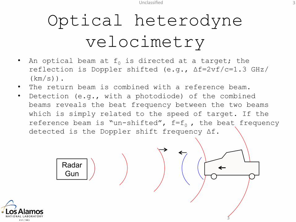
•  An optical beam at f0 is directed at a target; the reflection is Doppler shifted (e.g., Δf=2vf/c=1.3 GHz/(km/s)).

•  The return beam is combined with a reference beam. •  Detection (e.g., with a photodiode) of the combined

beams reveals the beat frequency between the two beams which is simply related to the speed of target. If the reference beam is “un-shifted”, f=f0 , the beat frequency detected is the Doppler shift frequency Δf.

Radar Gun

Unclassified   4  

Attributes of optical heterodyne velocimetry

1. Unambiguous interpretation: measures the component of scatterer velocity along the beam, vscatterer* cos(θ).

2. Capable of high bandwidth. 3. Robust extraction of signal from

noise with sliding power spectrum. 4. Can measure multiple velocities

simultaneously. 5. Can measure the bulk velocity of a

cloud of particles – in principle, no solid surface required.

4

Unclassified   5  

5

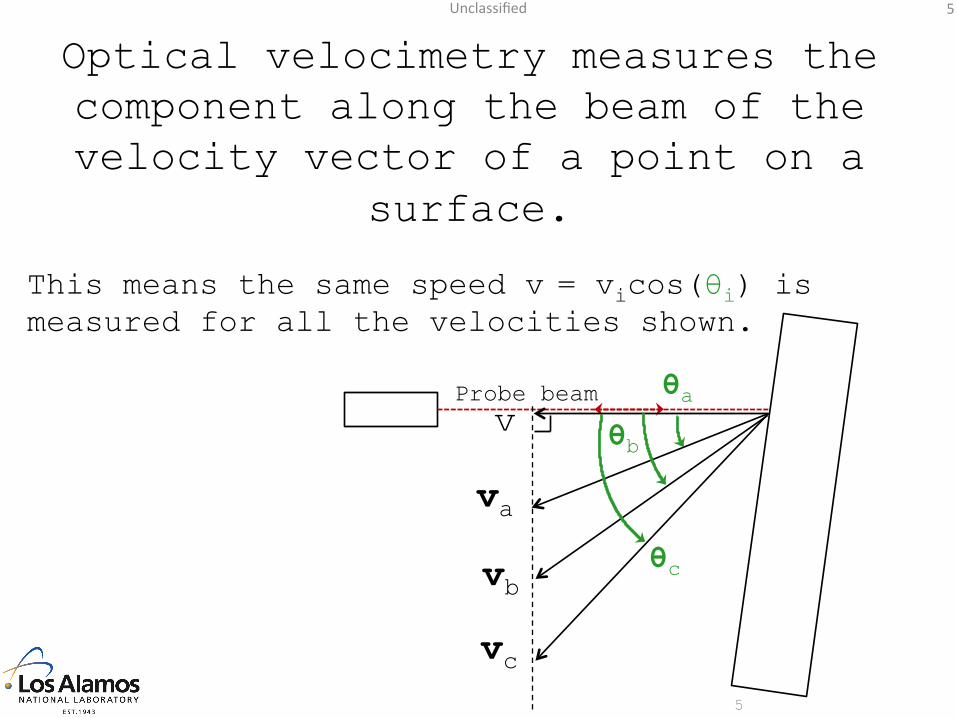
Optical velocimetry measures the component along the beam of the velocity vector of a point on a

surface.

vb

θa

va

v

vc

θb

θc

This means the same speed v = vicos(θi) is measured for all the velocities shown.

Probe beam

Unclassified   6  

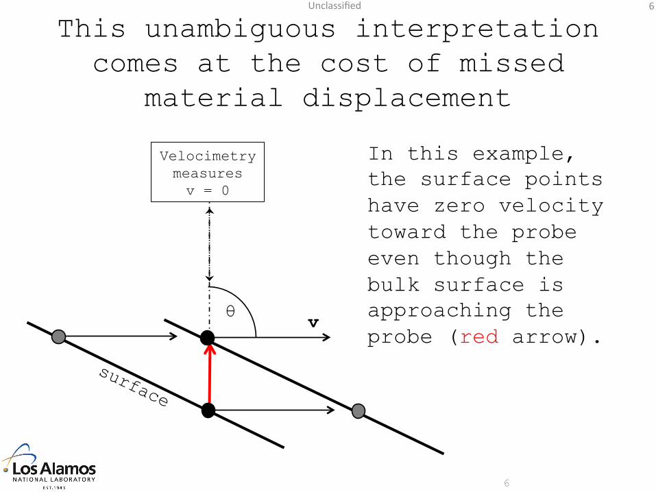
In this example, the surface points have zero velocity toward the probe even though the bulk surface is approaching the probe (red arrow).

6

θ v

This unambiguous interpretation comes at the cost of missed

material displacement

Velocimetry measures v = 0

Unclassified   7  

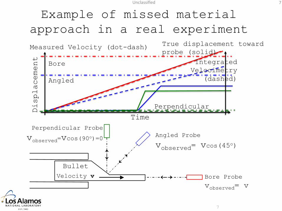
Example of missed material approach in a real experiment

7

Perpendicular Probe

vobserved=vcos(90o)=0 Angled Probe

vobserved= vcos(45o)

Bore Probe

vobserved= v

Bullet Velocity v

True displacement toward probe (solid)

Displacement

Measured Velocity (dot-dash)

Bore

Angled

Perpendicular

Time

Integrated Velocimetry

(dashed)

Unclassified   8  

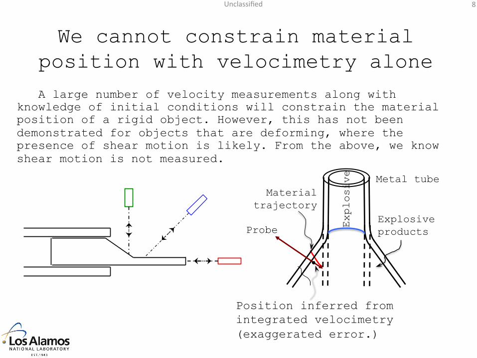
We cannot constrain material position with velocimetry alone

A large number of velocity measurements along with knowledge of initial conditions will constrain the material position of a rigid object. However, this has not been demonstrated for objects that are deforming, where the presence of shear motion is likely. From the above, we know shear motion is not measured.

Probe Explosive

Explosive products

Metal tube

Position inferred from integrated velocimetry (exaggerated error.)

Material trajectory

Unclassified   9  

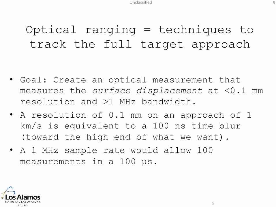
Optical ranging = techniques to track the full target approach

•  Goal: Create an optical measurement that measures the surface displacement at <0.1 mm resolution and >1 MHz bandwidth.

•  A resolution of 0.1 mm on an approach of 1 km/s is equivalent to a 100 ns time blur (toward the high end of what we want).

•  A 1 MHz sample rate would allow 100 measurements in a 100 µs.

9

Unclassified   10  

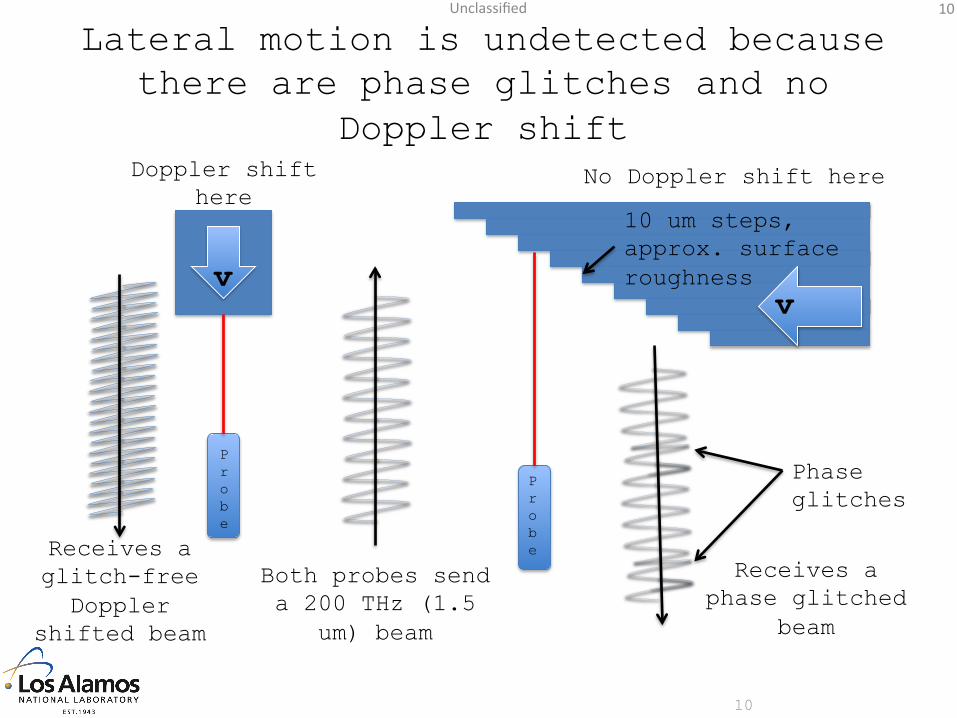
Lateral motion is undetected because there are phase glitches and no

Doppler shift

10

Both probes send a 200 THz (1.5

um) beam

Receives a glitch-free

Doppler shifted beam

Receives a phase glitched

beam

Phase glitches

Probe

Probe

10 um steps, approx. surface roughness

Doppler shift here

No Doppler shift here

v  v  

Unclassified   11  

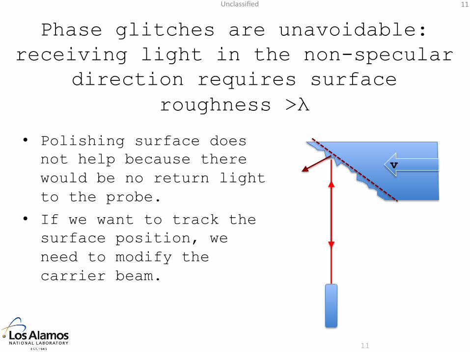
Phase glitches are unavoidable: receiving light in the non-specular

direction requires surface roughness >λ

•  Polishing surface does not help because there would be no return light to the probe.

•  If we want to track the surface position, we need to modify the carrier beam.

11

v  

Unclassified   12  

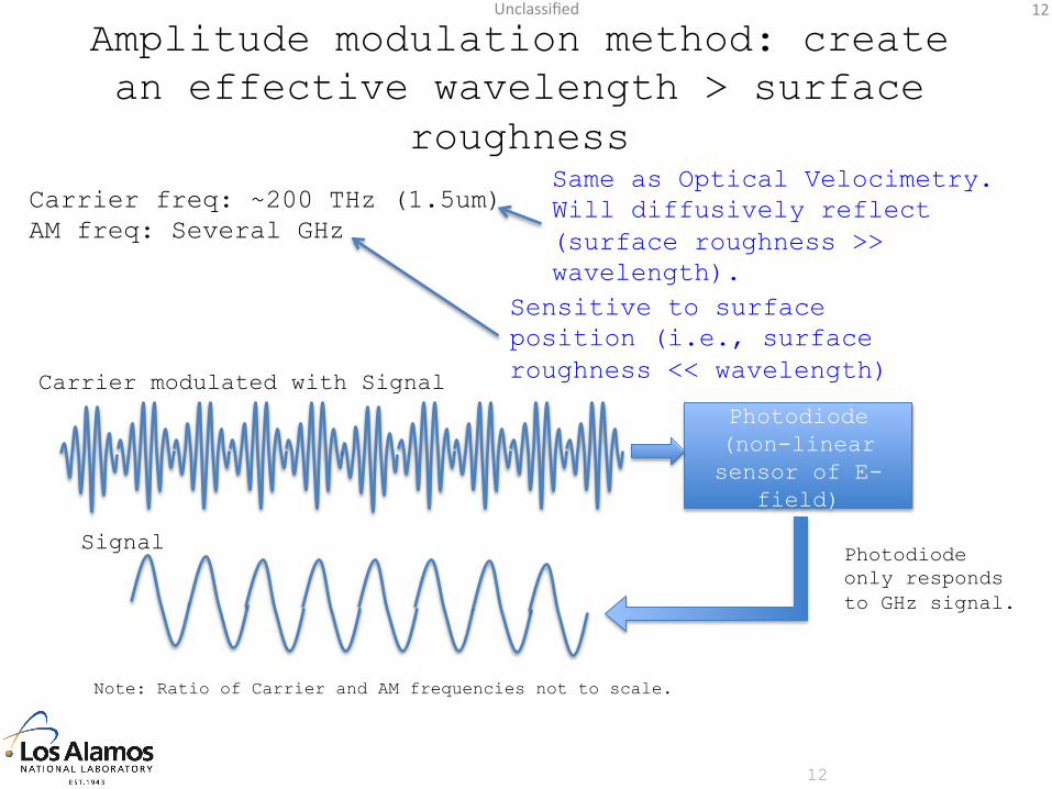
Amplitude modulation method: create an effective wavelength > surface

roughness

12

Carrier freq: ~200 THz (1.5um) AM freq: Several GHz

Photodiode (non-linear sensor of E-

field)

Photodiode only responds to GHz signal.

Same as Optical Velocimetry. Will diffusively reflect (surface roughness >> wavelength).

Sensitive to surface position (i.e., surface roughness << wavelength) Carrier modulated with Signal

Signal

Note: Ratio of Carrier and AM frequencies not to scale.

Unclassified   13  

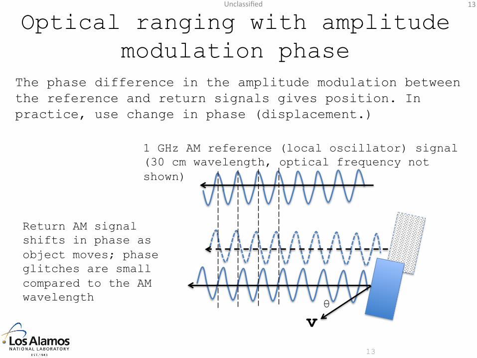
Optical ranging with amplitude modulation phase

The phase difference in the amplitude modulation between the reference and return signals gives position. In practice, use change in phase (displacement.)

13

1 GHz AM reference (local oscillator) signal (30 cm wavelength, optical frequency not shown)

Return AM signal shifts in phase as object moves; phase glitches are small compared to the AM wavelength

v  θ

Unclassified   14  

Optical Ranging Rules

•  Measurement Bandwidth: –  Upper limit is the AM frequency –  In practice, will average over many cycles (i.e., a GHz AM signal will give a MHz measurement bandwidth)

•  Resolution: –  Depends on Bandwidth of phase comparator, the AM freq., & signal/noise ratio at the AM freq.

–  Should be insensitive to noise at other frequencies.

Unclassified   15  

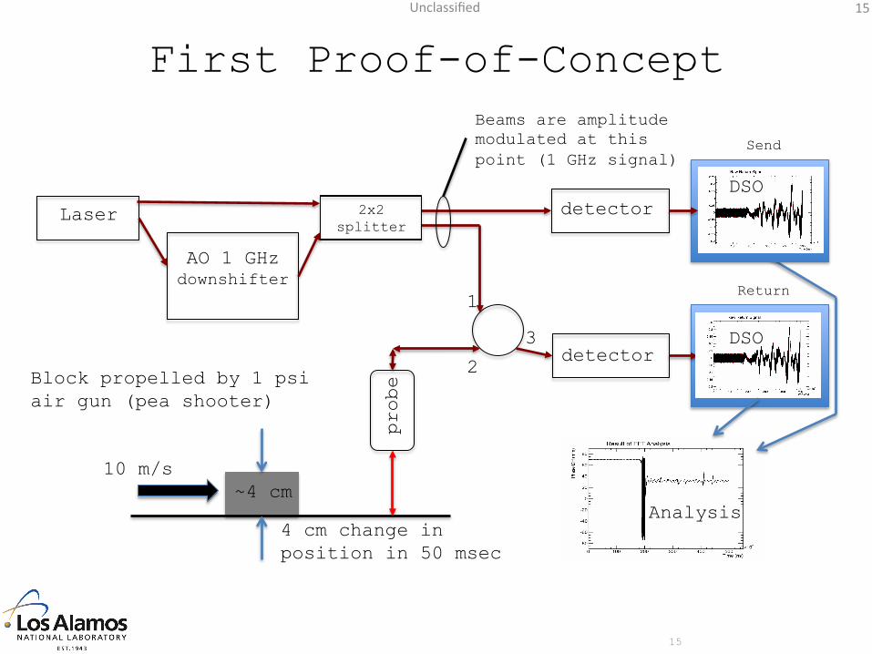
First Proof-of-Concept

15

probe

detector

detector Laser

AO 1 GHz downshifter

DSO 2x2

splitter

Beams are amplitude modulated at this point (1 GHz signal)

1

2

3

~4 cm 10 m/s

DSO

Analysis

Send

Return

Block propelled by 1 psi air gun (pea shooter)

4 cm change in position in 50 msec

Unclassified   16  

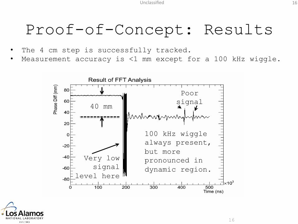
Proof-of-Concept: Results •  The 4 cm step is successfully tracked. •  Measurement accuracy is <1 mm except for a 100 kHz wiggle.

16

Very low signal

level here

Poor signal

100 kHz wiggle always present, but more pronounced in dynamic region.

40 mm

Unclassified   17  

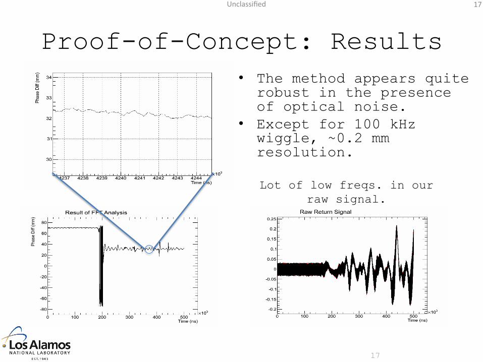
Proof-of-Concept: Results •  The method appears quite

robust in the presence of optical noise.

•  Except for 100 kHz wiggle, ~0.2 mm resolution.

17

Lot of low freqs. in our raw signal.

Unclassified   18  

Summary of amplitude modulation approach

•  The Optical Ranging method presented here complements Velocimetry and can coexist on the same probe with PDV.

•  Our initial proof-of-concept was successful, and we expect our resolution to improve.

18

Unclassified   19  

Slide 19

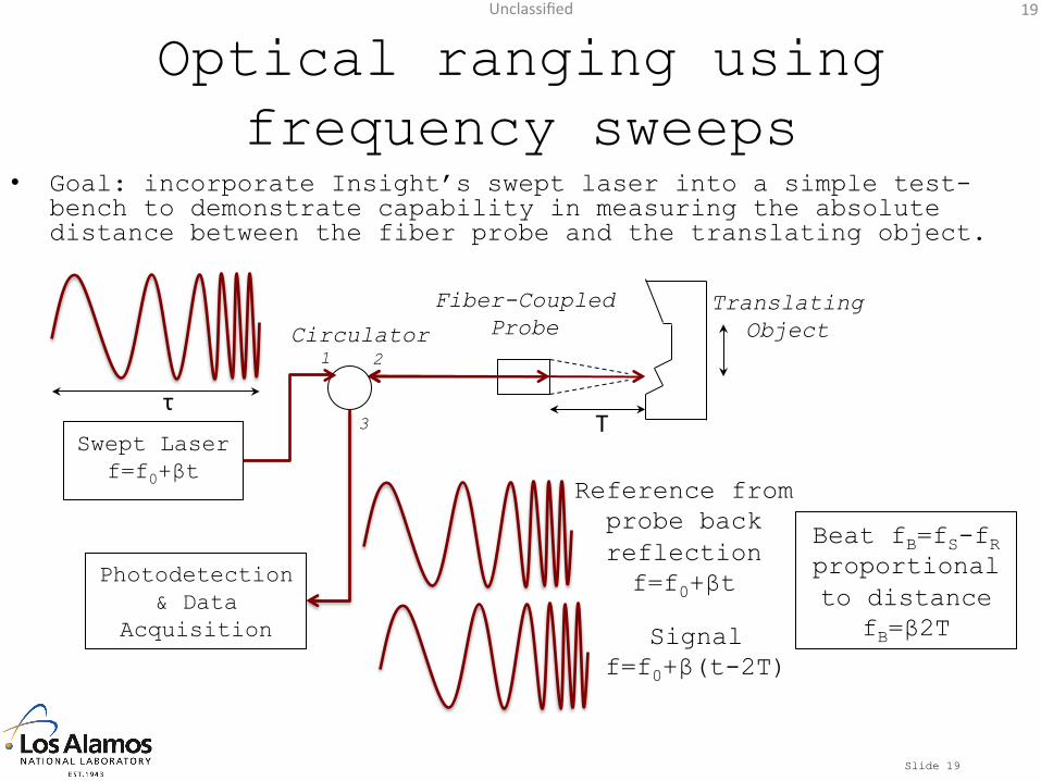
Optical ranging using frequency sweeps

•  Goal: incorporate Insight’s swept laser into a simple test-bench to demonstrate capability in measuring the absolute distance between the fiber probe and the translating object.

Fiber-Coupled Probe

Translating Object

Swept Laser f=f0+βt

Photodetection & Data

Acquisition

1 2

3

Circulator

Τ  τ  

Reference from probe back reflection f=f0+βt

Signal f=f0+β(t-2Τ)

Beat fB=fS-fR proportional to distance

fB=β2Τ

Unclassified   20  

Slide 20

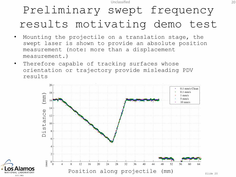
Preliminary swept frequency results motivating demo test

•  Mounting the projectile on a translation stage, the swept laser is shown to provide an absolute position measurement (note: more than a displacement measurement.)

•  Therefore capable of tracking surfaces whose orientation or trajectory provide misleading PDV results

0 4 8 12 16 20 24 28 32 36 40 44 48 52 56 60 640

2

4

6

8

10

12

14

16

18

20

0.1 mm/s Clean0.1 mm/s1 mm/s5 mm/s10 mm/s

0 4 8 12 16 20 24 28 32 36 40 44 48 52 56 60 640

2

4

6

8

10

12

14

16

18

20

0.1 mm/s1 mm/s5 mm/s10 mm/s

Horizontal Position (mm)

Hei

ght (

mm

)

Normal Probe, Forward Direction: Profile as a Function of Position, Determinedusing TimeïDomain Position Measurements & Known Velocity

Distance (mm)  

Position along projectile (mm)  

Unclassified   21  

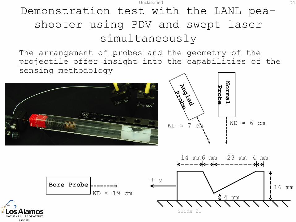
Demonstration test with the LANL pea-shooter using PDV and swept laser

simultaneously The arrangement of probes and the geometry of the projectile offer insight into the capabilities of the sensing methodology

Slide 21

14 mm 6 mm

16 mm

23 mm 4 mm

4 mm

+ v

Normal

Probe

Bore Probe

WD ≈ 6 cm WD ≈ 7 cm

WD ≈ 19 cm

Unclassified   22  

Slide 22

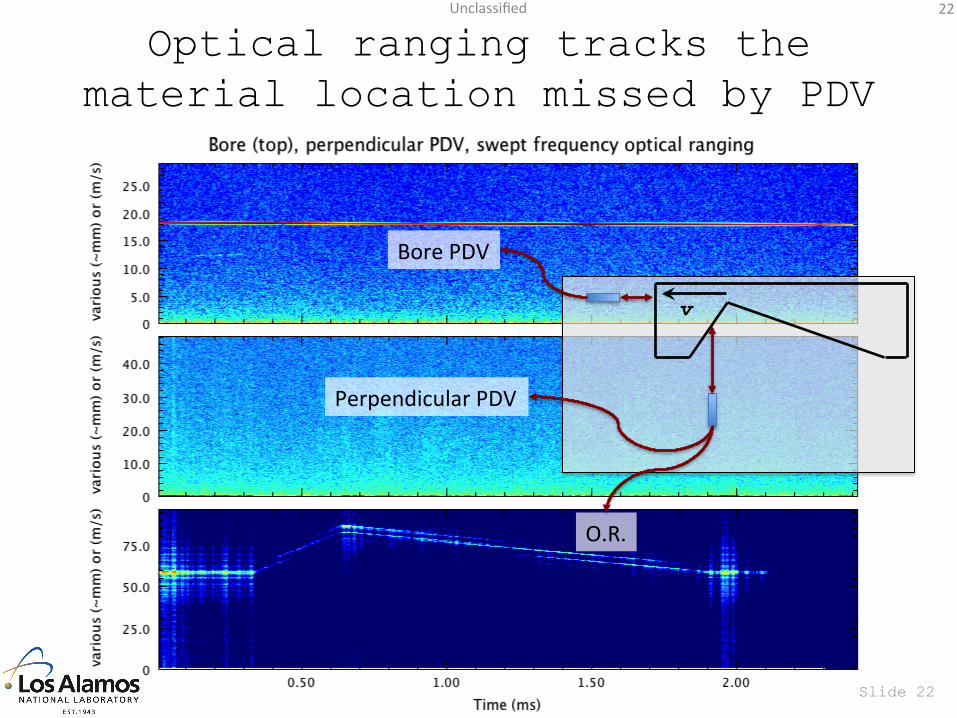
Optical ranging tracks the material location missed by PDV

Perpendicular  PDV  

O.R.  

Bore  PDV  

v

Unclassified   23  

Slide 23

Hardware Details – Insight Swept Laser

•  For our tests, the 10 mW laser’s wavelength swept over 1530-1550 nm (capable of larger sweeps, on the order of 100-200 nm) –  There is a tradeoff between wavelength range, sweep rate,

and the density at which the wavelength range is sampled •  Each complete sweep corresponds to a single position

measurement –  These wavelength sweeps took place at a rep rate of

138.50 kHz, generating a position measurement every 7.2 µs

–  2888 sample points per wavelength sweep (6.9 pm per point, over 20 nm), used to compare the laser’s wavelength to a NIST traceable gas reference cell

•  We sampled the optical signal at 50 Gigasamples/sec, compared to the laser’s 400 MHZ internal clock, so we measured the interferometer response between these traceable points

Unclassified   24  

Slide 24

Summary: 2 techniques have passed proof tests, 3rd promising simulations

•  The amplitude modulation approach of Younk will coexist with PDV and appears to have the required resolution. The difficulties inherent in phase measurements may be offset by averaging ~100 cycles per measurement.

•  Moro’s frequency swept approach coexists with PDV and is a frequency measurement rather than phase. The sweep takes 5 µs, which probably needs to be shortened substantially to avoid blur. Our colleagues at NSTec are working on this approach.

•  The amplitude-modulation beat-frequency approach proposed by Knierim promises continuous measurement that is frequency based. Tests on this are still needed.

•  All of these techniques appear compatible with integration into PDV or MPDV systems with minimal perturbation.

Unclassified   25  

Backups  

Unclassified   26  

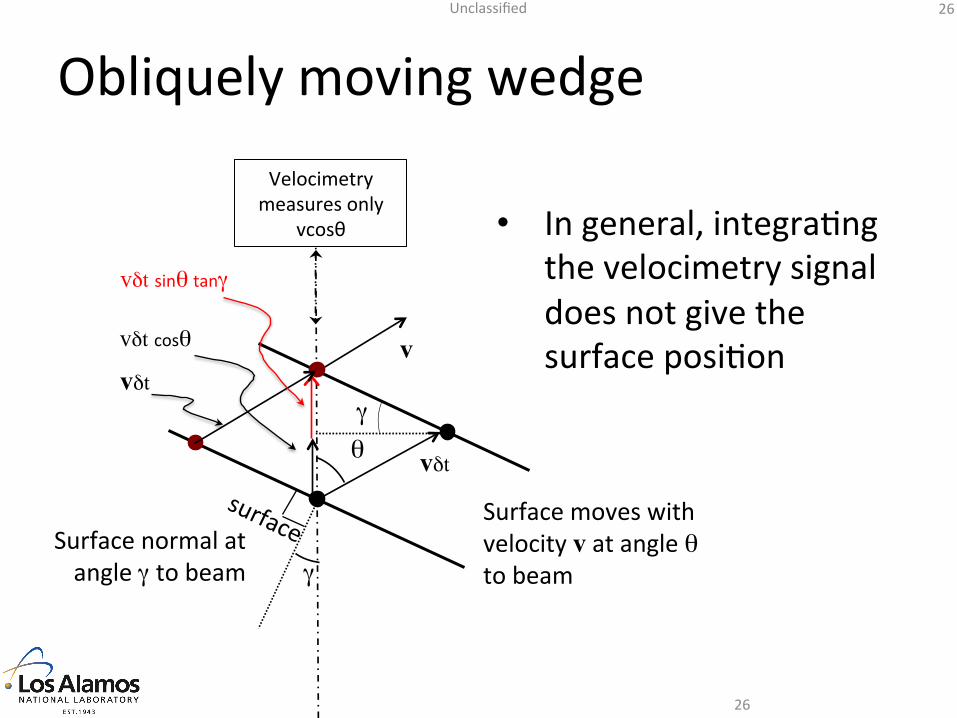
•  In  general,  integraHng  the  velocimetry  signal  does  not  give  the  surface  posiHon  

26  

θ

v

Surface  normal  at  angle  γ to  beam    

vδt

γ

Surface  moves  with  velocity  v  at  angle  θ to  beam    

Velocimetry  measures  only  

vcosθ  

vδt sinθ  tanγ

vδt cosθ

γ vδt

Obliquely  moving  wedge  

Unclassified   27  

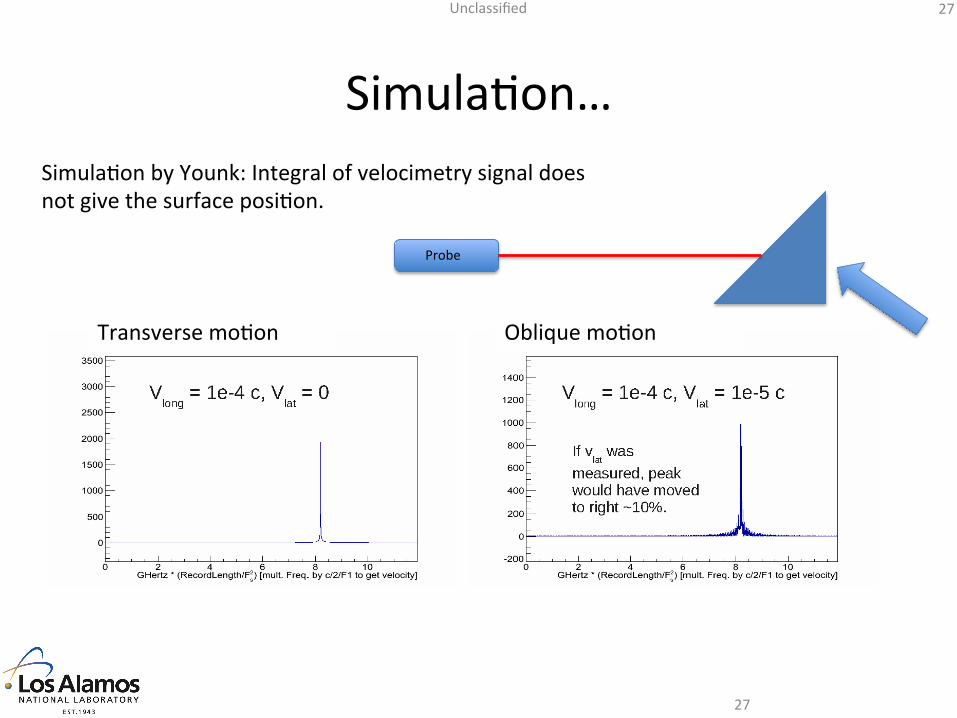
SimulaHon…  

27  

SimulaHon  by  Younk:  Integral  of  velocimetry  signal  does  not  give  the  surface  posiHon.  

Probe  

Oblique  moHon  Transverse  moHon  

Unclassified   28  

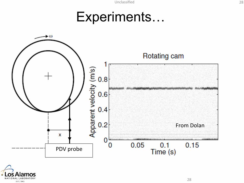
Experiments…

28  

PDV  probe  

From  Dolan  

Unclassified   29  

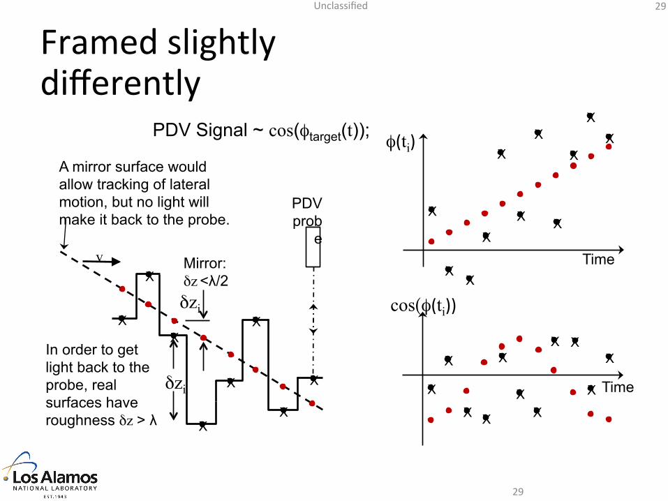
PDV Signal ~ cos(φtarget(t));

29  

X

X

X

X

X

X

X

X δzi

δzi

Mirror: δz <λ/2

v

A mirror surface would allow tracking of lateral motion, but no light will make it back to the probe.

PDV prob

e

In order to get light back to the probe, real surfaces have roughness δz > λ

X

X X

X

X X

X

X

X

X X φ(ti)  

Time

X

X

X

X

X

X X

X X

X

X

cos(φ(ti))  

Time

Framed  slightly    differently  

Unclassified   30  

We  need  to  know  the  locaHon  of  the  material  to  model  a  system  

30  

•  IntegraHng  the  velocity  measured  by  the  velocimetry  method  will  predict  a  smaller  radius  than  is  in  fact  present,  because  some  of  the  radial  moHon  arises  from  the  Hlted  surface  moving  axially.  

Probe  

Explosive  

Explosive  products  

Metal  tube  

Posi&on  inferred  from  integrated  velocimetry  (exaggerated  error.)  

Material  trajectory  

Unclassified   31  

The  OpHcal  Ranging  Principle  

•  The  phase  difference  between  the  send  and  return  THz  carriers  is  scrambled  by  the  surface  roughness.  

•  But  the  phase  difference  between  the  send  and  return  GHz  signals  tracks  surface  posiHon.  

 

31  

Unclassified   32  

Measuring  a  phase  difference…  

•  …is  different  from  measuring  a  frequency  difference.  

•  In  the  current  example,  if  we  let  the  send  and  return  signals  heterodyne,  the  beat  freq.  would  be  ~7  kHz  for  a  1  km/s  approach.  

 

32  

FYI:  Combining  these  raw  signals  and  measuring  the  beat  freq.  is  a  poor  measurement  of  velocity.  

Unclassified   33  

OpHcal  Ranging  Rules  

33  

180°  out  of  phase  

send  

send  

return  

return  

x  =  ¼  λ

0°  out  of  phase  

Scale  Rule:  Δφ  =  4π  x/λ

Unclassified   34  

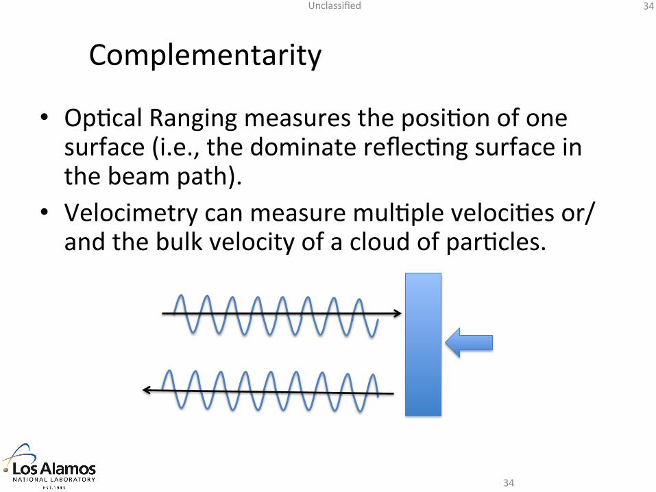
Complementarity  

•  OpHcal  Ranging  measures  the  posiHon  of  one  surface  (i.e.,  the  dominate  reflecHng  surface  in  the  beam  path).  

•  Velocimetry  can  measure  mulHple  velociHes  or/and  the  bulk  velocity  of  a  cloud  of  parHcles.  

34  

Unclassified   35  

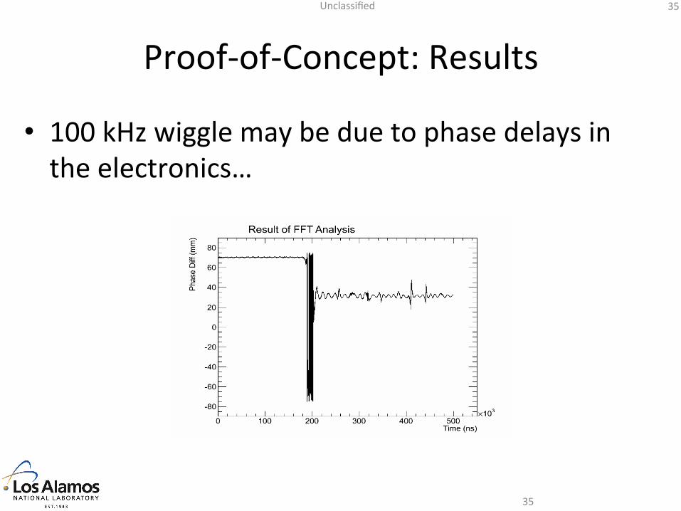
Proof-­‐of-­‐Concept:  Results  

•  100  kHz  wiggle  may  be  due  to  phase  delays  in  the  electronics…  

35  

Unclassified   36  

Points

•  Proof-of-Concept successful. •  We believe we understand the 100 kHz wiggle. It is straightforward to remove.

•  Currently we are at ~0.2 mm resolution and ~10 MHz bandwidth when the signal is reasonably strong.

•  This early success is promising.

36

Unclassified   37  

Variants: Creating the AM modulation

•  The AM signal can be made in different ways…

–  Combining two highly stable lasers. Their freq. difference is the AM freq.

–  FM modulating a laser beam and then recombining it with an un-modulated beam.

–  The recombining could be done before or after the beam is sent to the target.

•  Each method may have certain advantages…. we are investigating.

37

Unclassified   38  

Other Variants •  The phase comparison can be made digitally or with analog circuitry.

•  Doppler-shifted Velocimetry and Optical Ranging can co-exist on the same probe. –  This is of particular interest because of their aforementioned complementarity.

–  But there may be a cost to pay…. –  We may have to double the laser power to maintain the fidelity in PDV.

38