languagesandcomputation(g52lac) lecturenotes...
TRANSCRIPT
Languages and Computation (G52LAC)
Lecture notes
Spring 2018
Thorsten Altenkirch, Venanzio Capretta, and Henrik Nilsson
February 21, 2018
Contents
1 Introduction 41.1 Example: Valid Java programs . . . . . . . . . . . . . . . . . . . 41.2 Example: The halting problem . . . . . . . . . . . . . . . . . . . 51.3 Example: The λ-calculus . . . . . . . . . . . . . . . . . . . . . . . 61.4 P versus NP . . . . . . . . . . . . . . . . . . . . . . . . . . . . . . 7
2 Formal Languages 92.1 Exercises . . . . . . . . . . . . . . . . . . . . . . . . . . . . . . . 11
3 Finite Automata 133.1 Deterministic finite automata . . . . . . . . . . . . . . . . . . . . 13
3.1.1 What is a DFA? . . . . . . . . . . . . . . . . . . . . . . . 133.1.2 The language of a DFA . . . . . . . . . . . . . . . . . . . 15
3.2 Nondeterministic finite automata . . . . . . . . . . . . . . . . . . 163.2.1 What is an NFA? . . . . . . . . . . . . . . . . . . . . . . . 163.2.2 The language accepted by an NFA . . . . . . . . . . . . . 183.2.3 The subset construction . . . . . . . . . . . . . . . . . . . 213.2.4 Correctness of the subset construction . . . . . . . . . . . 25
3.3 Exercises . . . . . . . . . . . . . . . . . . . . . . . . . . . . . . . 26
4 Regular Expressions 294.1 What are regular expressions? . . . . . . . . . . . . . . . . . . . . 294.2 The meaning of regular expressions . . . . . . . . . . . . . . . . . 304.3 Algebraic laws . . . . . . . . . . . . . . . . . . . . . . . . . . . . 334.4 Translating regular expressions into NFAs . . . . . . . . . . . . . 344.5 Summing up . . . . . . . . . . . . . . . . . . . . . . . . . . . . . 444.6 Exercises . . . . . . . . . . . . . . . . . . . . . . . . . . . . . . . 45
5 Minimization of Finite Automata 465.1 The table-filling algorithm . . . . . . . . . . . . . . . . . . . . . . 465.2 Example of DFA minimization using the table-filling algorithm . 47
1
6 Disproving Regularity 506.1 The pumping lemma . . . . . . . . . . . . . . . . . . . . . . . . . 506.2 Applying the pumping lemma . . . . . . . . . . . . . . . . . . . . 516.3 Exercises . . . . . . . . . . . . . . . . . . . . . . . . . . . . . . . 52
7 Context-Free Grammars 537.1 What are context-free grammars? . . . . . . . . . . . . . . . . . . 537.2 The meaning of context-free grammars . . . . . . . . . . . . . . . 557.3 The relation between regular and context-free languages . . . . . 567.4 Derivation trees . . . . . . . . . . . . . . . . . . . . . . . . . . . . 577.5 Ambiguity . . . . . . . . . . . . . . . . . . . . . . . . . . . . . . . 597.6 Applications of context-free grammars . . . . . . . . . . . . . . . 627.7 Exercises . . . . . . . . . . . . . . . . . . . . . . . . . . . . . . . 64
8 Transformations of context-free grammars 668.1 Equivalence of context-free grammars . . . . . . . . . . . . . . . 668.2 Elimination of uselsss productions . . . . . . . . . . . . . . . . . 668.3 Substitution . . . . . . . . . . . . . . . . . . . . . . . . . . . . . . 678.4 Left factoring . . . . . . . . . . . . . . . . . . . . . . . . . . . . . 688.5 Disambiguating context-free grammars . . . . . . . . . . . . . . . 688.6 Elimination of left recursion . . . . . . . . . . . . . . . . . . . . . 708.7 Exercises . . . . . . . . . . . . . . . . . . . . . . . . . . . . . . . 74
9 Pushdown Automata 759.1 What is a pushdown automaton? . . . . . . . . . . . . . . . . . . 759.2 How does a PDA work? . . . . . . . . . . . . . . . . . . . . . . . 769.3 The language of a PDA . . . . . . . . . . . . . . . . . . . . . . . 779.4 Deterministic PDAs . . . . . . . . . . . . . . . . . . . . . . . . . 789.5 Context-free grammars and push-down automata . . . . . . . . . 79
10 Recursive-Descent Parsing 8110.1 What is parsing? . . . . . . . . . . . . . . . . . . . . . . . . . . . 8110.2 Parsing strategies . . . . . . . . . . . . . . . . . . . . . . . . . . . 8110.3 Basics of recursive-descent parsing . . . . . . . . . . . . . . . . . 8210.4 Handling choice . . . . . . . . . . . . . . . . . . . . . . . . . . . . 8510.5 Recursive-descent parsing and left-recursion . . . . . . . . . . . . 8810.6 Predictive parsing . . . . . . . . . . . . . . . . . . . . . . . . . . 88
10.6.1 First and follow sets . . . . . . . . . . . . . . . . . . . . . 9010.6.2 LL(1) grammars . . . . . . . . . . . . . . . . . . . . . . . 9010.6.3 Nullable nonterminals . . . . . . . . . . . . . . . . . . . . 9110.6.4 Computing first sets . . . . . . . . . . . . . . . . . . . . . 9210.6.5 Computing follow sets . . . . . . . . . . . . . . . . . . . . 9310.6.6 Implementing a predictive parser . . . . . . . . . . . . . . 9410.6.7 LL(1), left-recursion, and ambiguity . . . . . . . . . . . . 9610.6.8 Satisfying the LL(1) conditions . . . . . . . . . . . . . . . 98
10.7 Beyond hand-written parsers: use parser generators . . . . . . . . 9810.8 Exercises . . . . . . . . . . . . . . . . . . . . . . . . . . . . . . . 100
2
11 Turing Machines 10111.1 What is a Turing machine? . . . . . . . . . . . . . . . . . . . . . 10111.2 Grammars and context-sensitivity . . . . . . . . . . . . . . . . . 10411.3 The halting problem . . . . . . . . . . . . . . . . . . . . . . . . . 10511.4 Recursive and recursively enumerable sets . . . . . . . . . . . . . 10611.5 Back to Chomsky . . . . . . . . . . . . . . . . . . . . . . . . . . . 10911.6 Exercises . . . . . . . . . . . . . . . . . . . . . . . . . . . . . . . 110
12 λ-Calculus 11212.1 Syntax of λ-calculus . . . . . . . . . . . . . . . . . . . . . . . . . 11212.2 Church numerals . . . . . . . . . . . . . . . . . . . . . . . . . . . 11512.3 Other data structures . . . . . . . . . . . . . . . . . . . . . . . . 11612.4 Confluence . . . . . . . . . . . . . . . . . . . . . . . . . . . . . . 11712.5 Recursion . . . . . . . . . . . . . . . . . . . . . . . . . . . . . . . 11812.6 The universality of λ-calculus . . . . . . . . . . . . . . . . . . . . 11912.7 Exercises . . . . . . . . . . . . . . . . . . . . . . . . . . . . . . . 120
13 Algorithmic Complexity 12113.1 The Satisfiability Problem . . . . . . . . . . . . . . . . . . . . . . 12213.2 Time Complexity . . . . . . . . . . . . . . . . . . . . . . . . . . . 12213.3 NP-completeness . . . . . . . . . . . . . . . . . . . . . . . . . . . 12413.4 Exercises . . . . . . . . . . . . . . . . . . . . . . . . . . . . . . . 125
A Model Answers to Exercises 127
List of exercises
Exercise 2.1 . . . . . . . . . . . . . . . . . . . . . . . . . . . . . . . . 11Exercise 2.2 . . . . . . . . . . . . . . . . . . . . . . . . . . . . . . . . 12Exercise 3.1 . . . . . . . . . . . . . . . . . . . . . . . . . . . . . . . . 26Exercise 3.2 . . . . . . . . . . . . . . . . . . . . . . . . . . . . . . . . 26Exercise 3.3 . . . . . . . . . . . . . . . . . . . . . . . . . . . . . . . . 26Exercise 3.4 . . . . . . . . . . . . . . . . . . . . . . . . . . . . . . . . 27Exercise 3.5 . . . . . . . . . . . . . . . . . . . . . . . . . . . . . . . . 27Exercise 4.1 . . . . . . . . . . . . . . . . . . . . . . . . . . . . . . . . 45Exercise 4.2 . . . . . . . . . . . . . . . . . . . . . . . . . . . . . . . . 45Exercise 4.3 . . . . . . . . . . . . . . . . . . . . . . . . . . . . . . . . 45Exercise 6.1 . . . . . . . . . . . . . . . . . . . . . . . . . . . . . . . . 52Exercise 7.1 . . . . . . . . . . . . . . . . . . . . . . . . . . . . . . . . 64Exercise 7.2 . . . . . . . . . . . . . . . . . . . . . . . . . . . . . . . . 64Exercise 7.3 . . . . . . . . . . . . . . . . . . . . . . . . . . . . . . . . 64Exercise 7.4 . . . . . . . . . . . . . . . . . . . . . . . . . . . . . . . . 65Exercise 8.1 . . . . . . . . . . . . . . . . . . . . . . . . . . . . . . . . 74Exercise 8.2 . . . . . . . . . . . . . . . . . . . . . . . . . . . . . . . . 74Exercise 10.1 . . . . . . . . . . . . . . . . . . . . . . . . . . . . . . . 100Exercise 11.1 . . . . . . . . . . . . . . . . . . . . . . . . . . . . . . . 110Exercise 11.2 . . . . . . . . . . . . . . . . . . . . . . . . . . . . . . . 110Exercise 11.3 . . . . . . . . . . . . . . . . . . . . . . . . . . . . . . . 111Exercise 12.1 . . . . . . . . . . . . . . . . . . . . . . . . . . . . . . . 120
3

Exercise 12.2 . . . . . . . . . . . . . . . . . . . . . . . . . . . . . . . 120Exercise 13.1 . . . . . . . . . . . . . . . . . . . . . . . . . . . . . . . 125Exercise 13.2 . . . . . . . . . . . . . . . . . . . . . . . . . . . . . . . 125Exercise 13.3 . . . . . . . . . . . . . . . . . . . . . . . . . . . . . . . 126
1 Introduction
This module is about two fundamental notions in computer science, languagesand computation, and how they are related. Specific topics include:
• Automata Theory
• Formal Languages
• Models of Computation
• Complexity Theory
The module starts with an investigation of classes of formal languages andrelated abstract machines, considers practical uses of this theory such as parsing,and finishes with a discussion on what computation is, what can and cannot becomputed at all, and what can be computed efficiently, including famous resultssuch as the Halting Problem and open problems such as P versus NP.
G52LAC builds on G51MSC Mathematics for Computer Scientists and partsof G52ACE Algorithms Correctness and Efficiency. It feeds into modules suchas G53CMP Compilers, G53COM Computability, and G54FOP MathematicalFoundations of Programming. To give you a more concrete idea about what youwill encounter in this module, as well as the broader significance of the moduleand a bit of historical context, we will illustrate with some examples.
1.1 Example: Valid Java programs
Consider the following Java fragment:
class Foo {int n;
void printNSqrd() {System.out.println(n * n);
}}
As written using a text editor or as stored in a file, it is just a string of characters.But not any string is a valid Java program. For example, Java uses specifickeywords, have rules for what identifiers must look like, and requires propernesting, such as a definition of a method inside a definition of a class.
This raises a number of questions:
• How to describe the set of strings that are valid Java programs?
• Given a string, how to determine if it is a valid Java program or not?
• How to recover the structure of a Java program from a “flat” string?
4
To answer such questions, we will study regular expressions and grammars togive precise descriptions of languages, and various kinds of automata to decide ifa string belongs to a language or not. We will also consider how to systematicallyderive programs that efficiently answer this type of questions, drawing directlyfrom the theory. Such programs are key parts of compilers, web browsers andweb servers, and in fact of any program that uses structured text in one way oranother.
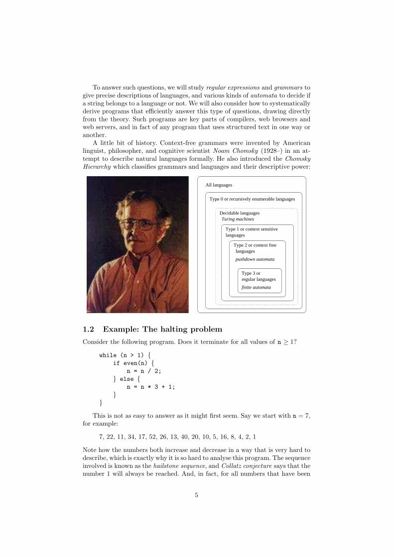
A little bit of history. Context-free grammars were invented by Americanlinguist, philosopher, and cognitive scientist Noam Chomsky (1928–) in an at-tempt to describe natural languages formally. He also introduced the ChomskyHierarchy which classifies grammars and languages and their descriptive power:
languages
finite automata
pushdown automata
Type 2 or context free
Type 3 orregular languages
Type 1 or context sensitive languages
Decidable languagesTuring machines
Type 0 or recursively enumerable languages
All languages
1.2 Example: The halting problem
Consider the following program. Does it terminate for all values of n ≥ 1?
while (n > 1) {if even(n) {
n = n / 2;
} else {n = n * 3 + 1;
}}
This is not as easy to answer as it might first seem. Say we start with n = 7,for example:
7, 22, 11, 34, 17, 52, 26, 13, 40, 20, 10, 5, 16, 8, 4, 2, 1
Note how the numbers both increase and decrease in a way that is very hard todescribe, which is exactly why it is so hard to analyse this program. The sequenceinvolved is known as the hailstone sequence, and Collatz conjecture says that thenumber 1 will always be reached. And, in fact, for all numbers that have been
5

tried (all numbers up to 260!), the sequence does indeed terminate. But so far,no one has been able to prove that it always will! The famous mathematicianPaul Erdos even said: “Mathematics may not be ready for such problems.” (SeeCollatz conjecture, Wikipedia.)
The following important decidability result should then perhaps not comeas a total surprise:
It is impossible to write a program that decides if another, arbitrary,program terminates (halts) or not.
This is known as the Halting Problem and it is thus one example of an undecid-able problem: the answer cannot be determined mechanically in general1.
The undecidability of the Halting Problem was first proved by British math-ematician, logician, and computer scientist Alan Turing (1912–1954):
Turing proved this result using Turing Machines, an abstract model of compu-tation that he introduced in 1936 to give a precise definition of what problemsare “effectively calculable” (can be solved mechanically). Turing was further in-strumental in the success of British code breaking efforts during World War IIand is also famous for the Turing test to decide if a machine exhibits intelligentbehaviour equivalent to, or indistinguishable from, that of a human. AndrewHodges has written a very good biography of Turing: Alan Turing: the Enigma(http://www.turing.org.uk/turing/).
1.3 Example: The λ-calculus
The λ-calculus is a theory of pure functions. It is very simple, having only twoconstructs: definition and application of functions. The folloing is an exampleof a λ-calculus term:
(λx.x)(λy.y)
1 This does not mean that it is impossible to compute the answer for every instance ofsuch a problem. On the contrary, in specific cases, the answer can often be computed veryeasily, and programs that attempt to solve undecidable problems can be very useful. But ifwe do write such a program, we must necessarily be prepared to give up one way or anotherwith a “don’t know” answer.
6

Like Turing machines, the λ-calculus is a universal model of computation. Itwas introduced by American mathematician and logician Alonzo Church (1903–1995), also in 1936, a little earlier than Turing’s machine:
Alan Turing subsequently became a PhD student of Alonzo Church. They provedthat Turing machines and the λ-calculus are equivalent in terms of computa-tional expressiveness. In fact, all proposed universal models of computation todate have proved to be equivalent in that sense. This is captured by the Church-Turing thesis :
What is effectively calculable is exactly what can be computed by aTuring machine.
Functional programming languages, like Haskell, and many proof assistantsimplement (variations of) the λ-calculus. This is thus an example of a theorywith very direct and practical applications.
1.4 P versus NP
Here is a seemingly innocuous question:
Can every problem whose solution can be checked quickly by a com-puter also be solved quickly by a computer?”
“Quickly” here means in time proportional to a polynomial in the size of theproblem. Whether or not this is ths case is known as the P versus NP problemand it is likely the most famous open problem in computer science, dating backto the 1950s. Here, “P” refers to the class of problems that can be solved inpolynomial time, while “NP” refers to problems that can be solved in nonde-terministic polynomial time, and the question is thus whether these two classesof problems actually are the same, or P = NP.
7

There is an abundance of important problems where solutions can be checkedquickly, but where the best known algorithm for finding a solution is exponentialin the size of the problem.
As an example, here is one, the Subset Sum Problem: Does some nonemptysubset of given set of integers sum to zero? For example, given {3,−2, 8,−5, 4, 9},the nonempty subset {−5,−2, 3, 4} sums to 0.
It is easy to check a proposed solution: just add all the numbers. If the initialset contains n integers, any proposed solution (being a subset) contains at mostn integers, so we can sum all the elements with at most n additions meaningthe total time taken is proportional to n (assuming addition is a constant timeoperation).
However, for finding a solution, no better way is known than essentiallychecking each possible subset one after another. As there are 2n subsets of a setwith n elements, this means finding a solution takes exponential time.
Whether or not there is a better way to solve the Subset Sum Problemmight not seem particularly important, but if it were the case that P = NP,then this would have monumental practical implications. For example, publickey cryptography, on which pretty much all secure Internet communication, suchas HTTPS, hinges, would no longer provide adequate security, and the entireInternet security infrastructure would have to be redesigned and reimplemented.The question here is if it is possible to quickly find the prime factors of (very)large numbers. As long as that is not the case, public key cryptography isconsidered secure.
8
2 Formal Languages
In this course we will use the terms language and word in a different way thanin everyday language:
• A language is a set of words.
• A word is a sequence, or string, of symbols.
We will write ǫ for the empty word; i.e., a sequence of length 0.This leaves us with the question: what is a symbol? The answer is: anything,
but it has to come from an alphabet Σ that is a finite set. A common (andimportant) instance is Σ = {0, 1}. Note that ǫ will never be a symbol to avoidconfusion.
Mathematically we say: Given an alphabet Σ we define the set Σ∗ as set ofwords (or sequences) over Σ: the empty word ǫ ∈ Σ∗ and given a symbol x ∈ Σand a word w ∈ Σ∗ we can form a new word xw ∈ Σ∗. These are all the wayselements on Σ∗ can be constructed (this is called an inductive definition). Thisunary ∗-operator is known as the Kleene star (or Kleene operator or Kleeneclosure).
With Σ = {0, 1}, typical elements of Σ∗ are 0010, 00000000,ǫ. Note, that weonly write ǫ if it appears on its own, instead of 00ǫ we just write 00.
Note further that Σ∗ by definition is always nonempty as the empty word ǫbelongs to Σ∗ for any alphabet Σ, including Σ = ∅. Moreover, for any nonemptyalphabet Σ, Σ∗ is an infinite set.
It is important to realise that although there are infinitely many words overa nonempty alphabet Σ, each word has a finite length. At first this may seemstrange: how can it be that all elements of a set with infinitely many elementscan be finite? A good way to think of an infinite set is as a process that cangenerate a new element whenever we need one, as many times as we like2. Buteach such element can obviously be of finite size as we at any point in timewill only have asked for finitely many elements. Conversely, if we make a setcontaining a single (notionally) “infinite” element, such as a number ∞ largerthan any number except itself, or an infinitely long string, that does not makethe set itself infinite: it would still contain exactly one element.
We can now define the notion of a language L over an alphabet Σ precisely:L ⊆ Σ∗ or equivalently L ∈ P(Σ∗)3.
Here are some informal examples of languages:
• The set {0010, 00000000, ǫ} is a language over Σ = {0, 1}. This is anexample of a finite language.
• The set of words with odd length over Σ = {1}.
• The set of words that contain the same number of 0s and 1s is a languageover Σ = {0, 1}.
2 Indeed, this is exactly how infinite data structures, such as infinite lists, are realised inlazy languages like Haskell.
3 Given a set A, P(A) is the powerset of A; that is, the set of all possible subsets of A. Forexample, if A = {a, b}, then P(A) = { ∅, {a}, {b}, {a, b} }. The number of elements |A| of aset A, its cardinality, and the number of elements in its power set are related by |P(A)| = 2|A|.Hence powerset.
9
• The set of words that contain the same number of 0s and 1s modulo 2(i.e., both are even or odd) is a language over Σ = {0, 1}.
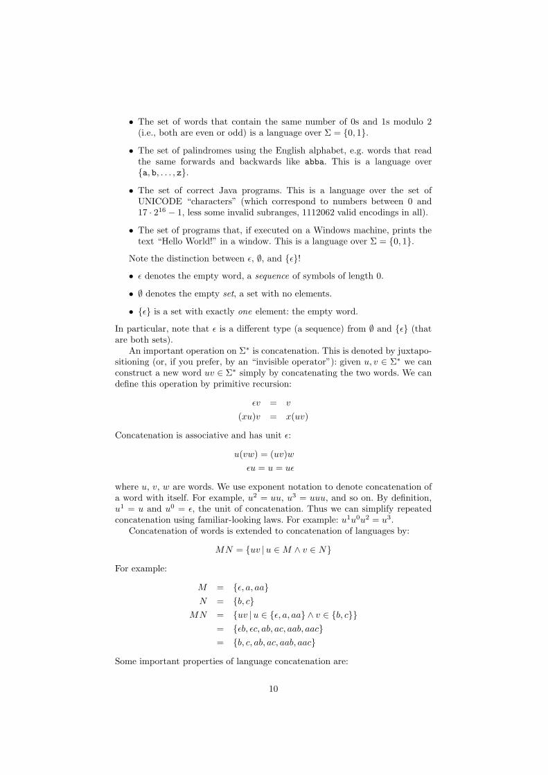
• The set of palindromes using the English alphabet, e.g. words that readthe same forwards and backwards like abba. This is a language over{a, b, . . . , z}.
• The set of correct Java programs. This is a language over the set ofUNICODE “characters” (which correspond to numbers between 0 and17 · 216 − 1, less some invalid subranges, 1112062 valid encodings in all).
• The set of programs that, if executed on a Windows machine, prints thetext “Hello World!” in a window. This is a language over Σ = {0, 1}.
Note the distinction between ǫ, ∅, and {ǫ}!
• ǫ denotes the empty word, a sequence of symbols of length 0.
• ∅ denotes the empty set, a set with no elements.
• {ǫ} is a set with exactly one element: the empty word.
In particular, note that ǫ is a different type (a sequence) from ∅ and {ǫ} (thatare both sets).
An important operation on Σ∗ is concatenation. This is denoted by juxtapo-sitioning (or, if you prefer, by an “invisible operator”): given u, v ∈ Σ∗ we canconstruct a new word uv ∈ Σ∗ simply by concatenating the two words. We candefine this operation by primitive recursion:
ǫv = v
(xu)v = x(uv)
Concatenation is associative and has unit ǫ:
u(vw) = (uv)w
ǫu = u = uǫ
where u, v, w are words. We use exponent notation to denote concatenation ofa word with itself. For example, u2 = uu, u3 = uuu, and so on. By definition,u1 = u and u0 = ǫ, the unit of concatenation. Thus we can simplify repeatedconcatenation using familiar-looking laws. For example: u1u0u2 = u3.
Concatenation of words is extended to concatenation of languages by:
MN = {uv |u ∈ M ∧ v ∈ N}
For example:
M = {ǫ, a, aa}
N = {b, c}
MN = {uv |u ∈ {ǫ, a, aa} ∧ v ∈ {b, c}}
= {ǫb, ǫc, ab, ac, aab, aac}
= {b, c, ab, ac, aab, aac}
Some important properties of language concatenation are:
10

• Concatenation of languages is associative:
L(MN) = (LM)N
• Concatenation of languages has zero ∅:
L∅ = ∅ = ∅L
• Concatenation of languages has unit {ǫ}:
L{ǫ} = L = {ǫ}L
• Concatenation distributes through set union:
L(M ∪N) = LM ∪ LN
(L ∪M)N = LN ∪MN
Note that concatenation does not distribute through intersection! Coun-terexample. Let L = {ǫ, a}, M = {ǫ}, N = {a}. Then:
L(M ∩N) = L∅ = ∅LM ∩ LN = {ǫ, a} ∩ {a, aa} = {a}
Exponent notation is used to denote iterated language concatenation: L1 = L,L2 = LL, L3 = LLL, and so on. By definition, L0 = {ǫ} (for any language,including ∅), which is the unit for language concatenation (just as u0 = ǫ is theunit for concatenation of words).
The Kleene star can also be applied to languages. This intuitively meanslanguage concatenation iterated 0 or more times:
L∗ =∞⋃
n=0
Ln
Note that ǫ ∈ L∗ for any language L, including L = ∅, the empty language. Asan example, if L = {a, ab}, then L∗ = {ǫ, a, ab, aab, aba, aaab, aaba, . . . }.
Alternatively (and more abstractly), L∗ can be described as the least lan-guage (with respect to ⊆) that contains L and the empty word, ǫ, and is closedunder concatenation:
u ∈ L∗ ∧ v ∈ L∗ =⇒ uv ∈ L∗
Note the subtle difference between using the Kleene star on an alphabet Σ,a set of symbols, as in Σ∗, and on using the Kleene star on a language L ⊆ Σ∗,a set of words. While the result in both cases is a set of words, the types of thearguments to the two variants of the Kleene star operation differ.
2.1 Exercises
Exercise 2.1
Let the alphabet Σ = {3, 5, 7, 9}, and let the language L = {w |w ∈ Σ∗, 1 ≤|w| ≤ 2}. (If w is a word, |w| denotes the length of that word. If X is a finiteset, like an alphabet or finite language, |X | denotes the number of elements inthat set, its cardinality.) Answer the following questions:
11

1. Describe L in plain English.
2. Enumerate all the words in L.
3. In general, for an arbitrary alphabet Σ1 and 0 ≤ m ≤ n, how many wordsare there in the language L1 = {w |w ∈ Σ∗
1,m ≤ |w| ≤ n}? That is, writedown an expression for |L1|.
4. How many words would there be in L1 if Σ1 = Σ, m = 3, and n = 7?
Exercise 2.2
Let the alphabet Σ = {a, b, c} and let L1 = {ǫ, b, ac} and L2 = {a, b, ca} betwo languages over Σ. Enumerate the words in the following languages, showingyour calculations in some detail:
1. L3 = L1 ∪ L2
2. L4 = L1{ǫ}(L2 ∩ L1)
3. L5 = L3∅L4
12

3 Finite Automata
Finite automata correspond to a computer with a fixed finite amount of mem-ory4. We will introduce deterministic finite automata (DFA) first and then moveto nondeterministic finite automata (NFA). An automaton will accept certainwords (sequences of symbols of a given alphabet Σ) and reject others. The setof accepted words is called the language of the automaton. We will show thatthe class of languages that are accepted by DFAs and NFAs is the same.
3.1 Deterministic finite automata
3.1.1 What is a DFA?
A deterministic finite automaton (DFA) A = (Q,Σ, δ, q0, F ) is given by:
1. A finite set of states Q
2. A finite set of input symbols, the alphabet, Σ
3. A transition function δ ∈ Q× Σ → Q
4. An initial state q0 ∈ Q
5. A set of final states F ⊆ Q
The initial states are sometimes called start states, and the final states aresometimes called accepting states.
As an example consider the following automaton
D = ({q0, q1, q2}, {0, 1}, δD, q0, {q2})
where
δD = {((q0, 0), q1), ((q0, 1), q0), ((q1, 0), q1), ((q1, 1), q2), ((q2, 0), q2), ((q2, 1), q2)}
if we view a function as a set of argument-result pairs. Alternatively, we candefine it case by case:
δD(q0, 0) = q1
δD(q0, 1) = q0
δD(q1, 0) = q1
δD(q1, 1) = q2
δD(q2, 0) = q2
δD(q2, 1) = q2
A DFA may be more conveniently represented by a transition table. Thetransition table for the DFA D is:
δD 0 1
→ q0 q1 q0q1 q1 q2
∗ q2 q2 q2
4 However, that does not mean that finite automata are a good model of general purposecomputers. A computer with n bits of memory has 2n possible states. That is an absolutelyenormous number even for very modest memory sizes, say 1024 bits or more, meaning thatdescribing a computer using finite automata quickly becomes infeasible. We will encounter abetter model of computers later, the Turing Machines.
13

A transition table represents the transition function δ of a DFA; i.e., the valueof δ(q, x) is given by the row labelled q in the column labelled x. In addition,the initial state is identified by putting an arrow → to the left of it, and allfinal states are similarly identified by a star ∗. The inclusion of this additionalinformation makes a transition table a self-contained representation of a DFA.
Note that the initial state also can be final (accepting). For example, for avariation D′ of the DFA D where q0 also is final:
δD′ 0 1
→ ∗ q0 q1 q0q1 q1 q2
∗ q2 q2 q2
Another way to represent a DFA is through a transition diagram. The tran-sition diagram for the DFA D is:
q0 q1 q2
1
0
0
1
0, 1
The initial state is identified by an incoming arrow. Final states are drawn witha double outline. If δ(q, x) = q′ then there is an arrow from state q to q′ that islabelled x. For another example, here is the transition diagram for the DFA D′:
q0 q1 q2
1
0
0
1
0, 1
An alternative to the double outline for a final state is to use an outgoingarrow. Using that convention, the transition diagram for the DFA D is:
q0 q1 q2
1
0
0
1
0, 1
Here is an example of a larger DFA over the alphabet Σ = {a, b, c} repre-sented by a transition diagram:
A
B
C
D
E
F G
a
c
b
c
c
a
b
a
b
abb
ca
c
a
b
c
c
a
b
14

The states are named by capital letters this time for a bit of variation: Q ={A,B,C,D,E, F,G}. While it is common to use symbols qi, i ∈ N to namestates, we can pick any names we like. Another common choice is to use naturalnumbers; i.e., Q ⊂ N ∧Q is finite.
The representation of the above DFA as a transition table is:
δ a b c
→ A B C AB B D AC E C A
∗ D E C F∗ E B D F
F B C G∗ G B C F
3.1.2 The language of a DFA
We will now discuss how a DFA accepts or rejects words over its alphabet ofinput symbols. The set of words accepted by a DFA A is called the languageL(A) of the DFA. Thus, for a DFA A with alphabet Σ, L(A) ⊆ Σ∗.
To determine whether a word w ∈ L(A), the machine starts in its initialstate. Taking the DFA D above as an example, it would start in state q0. Weindicate the state of a DFA by underlining the state name:
q0 q1 q2
1
0
0
1
0, 1
Then, whenever an input symbol is read from w, the machine transitions toa new state by following the edge labelled with this symbol. Once all symbolsin the input word w have been read, the word is accepted if the state is final,meaning w ∈ L(A), otherwise the word is rejected, meaning w /∈ L(A).
To continue with the example, suppose w = 101. The machine D wouldthus first read 1 and transition to a new state by following the edge labelled 1.As that edge in this case forms a loop back to state q0, the machine D wouldtransition back into state q0:
q0 q1 q2
1
0
0
1
0, 1
The machine would then read 0 and transition to state q1 by following the edgelabelled 0. We indicate this by moving the mark along that edge to q1:
q0 q1 q2
1
0
0
1
0, 1
15

Finally, the machine would read the last 1 in the input word, moving to q2:
q0 q1 q2
1
0
0
1
0, 1
As q2 is a final state, the DFAD accepts the wordw = 101, meaning 101 ∈ L(D).In the same way, we can determine that 0 /∈ L(D), 110 /∈ L(D), but 011 ∈ L(D).Verify this. Indeed, a little bit of thought reveals that
L(D) = {w | w contains the substring 01}
To make the notion of the language of a DFA precise, we now give a formaldefinition of L(A). First we define the extended transition function δ ∈ Q×Σ∗ →
Q. Intuitively, δ(q, w) = q′ if the machine starting from state q ends up in state
q′ when reading the word w. Formally, δ is defined by primitive recursion:
δ(q, ǫ) = q (1)
δ(q, xw) = δ(δ(q, x), w) (2)
where x ∈ Σ and w ∈ Σ∗. Thus, xw stands for a nonempty word the first symbolof which is x and the rest of which is w. For example, if xw = 010, then x = 0and w = 10. Note that w may be empty; e.g., if xw = 0, then x = 0 and w = ǫ.
As an example, we calculate δD(q0, 101) = q1:
δD(q0, 101) = δD(δD(q0, 1), 01) by (2)
= δD(q0, 01) because δD(q0, 1) = q0= δD(δD(q0, 0), 1) by (2)
= δD(q1, 1) because δD(q0, 0) = q1= δD(δD(q1, 1), ǫ) by (2)
= δD(q2, ǫ) because δD(q1, 1) = q2= q2 by (1)
Using the extended transition function δ, we define the language L(A) of aDFA A formally:
L(A) = {w | δ(q0, w) ∈ F}
Returning to our example, we thus have that 101 ∈ L(D) because δD(q0, 101) =q2 and q2 ∈ FD.
3.2 Nondeterministic finite automata
3.2.1 What is an NFA?
Nondeterministic finite automata (NFA) have transition functions that map agiven state and an input symbol to zero or more successor states. We can thinkof this as the machine having a “choice” whenever there are two or more possibletransitions from a state on an input symbol. In this presentation, we will further
16

allow an NFA to have more than one initial state5. Again, we can think of thisas the machine having a “choice” of where to start. An NFA accepts a word wif there is at least one possible way to get from one of the initial states to oneof the final states along edges labelled with the symbols of w in order.
It is important to note that although an NFA has a nondetermistic transitionfunction, it can always be determined whether or not a word belongs to itslanguage. Indeed, we shall see that every NFA can be translated into an DFAthat accepts the same language.
Here is an example of an NFA C that accepts all words over Σ = {0, 1} suchthat the symbol before the last is 1:
q0 q1 q2
0, 1
1 0, 1
A nondeterministic finite automaton (NFA) A = (Q,Σ, δ, S, F ) is given by:
1. A finite set of states Q,
2. A finite set of input symbols, the alphabet, Σ,
3. A transition function δ ∈ Q× Σ → P(Q),
4. A set of initial states S ⊆ Q,
5. A set of final (or accepting) states F ⊆ Q.
Thus, in contrast to a DFA, an NFA may have many initial states, not just one,and its transition function maps a state and an input symbol to a set of possiblesuccessor states, not just a single state. As an example we have that
C = ({q0, q1, q2}, {0, 1}, δC, {q0}, {q2})
where δC is given byδC 0 1
→ q0 {q0} {q0, q1}q1 {q2} {q2}
∗ q2 ∅ ∅
Note that the entries in the table are sets of states, and that these sets maybe empty (∅), here exemplified by the entries for state q2. Again, the (in thiscase only) initial state has been marked with → and the (in this case only) finalstate marked with ∗ to make this a self-contained representation of the NFA.
Here is another example of an NFA, this time over the alphabet Σ = {a, b, c}and with states Q = {0, 1, 2, 3, 4, 5} ⊂ N:
5 Note that we diverge slightly from the definition in the book [HMU01], which uses asingle initial state instead of a set of initial states. Permitting more than one initial stateallows us to avoid introducing ǫ-NFAs (see [HMU01], section 2.5).
17

0
1
2
3 4 5
a
b
b
a
a
b
c
a, b
a, b
c
c
The transition table for this NFA is:
δ a b c
→ 0 {1} {2} ∅∗ 1 {4} {3, 4} ∅∗ 2 {3, 4} {4} ∅
3 {1} {2} {3}→ ∗ 4 ∅ ∅ {5}
5 ∅ ∅ {4}
Note that this NFA has multiple initial states, multiple final states, one initialstate that also is final, and that there in some cases are no possible successorstates and in other cases more than one.
3.2.2 The language accepted by an NFA
To see whether a word w ∈ Σ∗ is accepted by an NFA A, we have to considerall possible states the machine could be in after having read a sequence of inputsymbols. Initially, an NFA can be in any of its initial states. Each time an inputsymbol is read, all successor states on the read symbol for each current possiblestate become the new possible states. After having read a complete word w, if atleast one of the possible states is final (accepting), then that word is accepted,meaning w ∈ L(A), otherwise it is rejected, meaning w /∈ L(A).
We will illustrate by showing how the NFA C rejects the word 100. We willagain mark the current states of the NFA by underlining the state names, butthis time there may be more than one marked state at once. Initially, as q0 isthe only initial state, we would have:
q0 q1 q2
0, 1
1 0, 1
Each time when we read a symbol we look at all the marked states. Weremove the old markers and put markers at all the states that are reachable viaan arrow marked with the current input symbol. This may include one or morestates that were marked previously. It may also be the case that no states arereachable, in which case all marks are removed and the word rejected (as it nolonger is possible to reach any final states). In our example, after reading 1,there would be two marked states as there are two arrows from q0 labelled 1:
q0 q1 q2
0, 1
1 0, 1
18
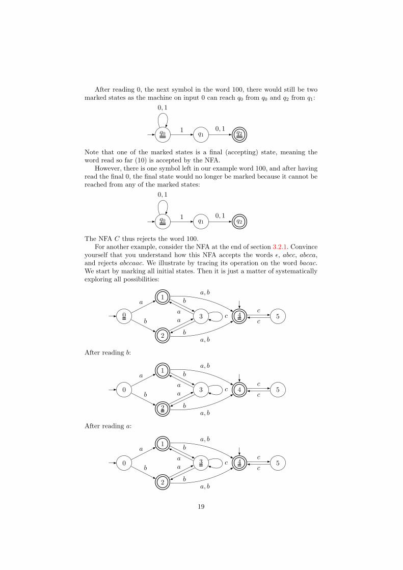
After reading 0, the next symbol in the word 100, there would still be twomarked states as the machine on input 0 can reach q0 from q0 and q2 from q1:
q0 q1 q2
0, 1
1 0, 1
Note that one of the marked states is a final (accepting) state, meaning theword read so far (10) is accepted by the NFA.
However, there is one symbol left in our example word 100, and after havingread the final 0, the final state would no longer be marked because it cannot bereached from any of the marked states:
q0 q1 q2
0, 1
1 0, 1
The NFA C thus rejects the word 100.For another example, consider the NFA at the end of section 3.2.1. Convince
yourself that you understand how this NFA accepts the words ǫ, abcc, abcca,and rejects abccaac. We illustrate by tracing its operation on the word bacac.We start by marking all initial states. Then it is just a matter of systematicallyexploring all possibilities:
0
1
2
3 4 5
a
b
b
a
a
b
c
a, b
a, b
c
c
After reading b:
0
1
2
3 4 5
a
b
b
a
a
b
c
a, b
a, b
c
c
After reading a:
0
1
2
3 4 5
a
b
b
a
a
b
c
a, b
a, b
c
c
19

After reading c:
0
1
2
3 4 5
a
b
b
a
a
b
c
a, b
a, b
c
c
After reading a:
0
1
2
3 4 5
a
b
b
a
a
b
c
a, b
a, b
c
c
After reading c:
0
1
2
3 4 5
a
b
b
a
a
b
c
a, b
a, b
c
c
The machine thus rejects bacac as no final state is marked. In fact, as there areno marked states left at all, this shows that this NFA will reject all words thatstart bacac. Can you find other such prefixes?
To define the extended transition function δ for NFAs we use a generalisationof the union operation ∪ on sets over a (finite) set of sets:
⋃
{A1, A2, . . . An} = A1 ∪A2 ∪ · · · ∪ An
In the special cases of the empty set of sets and a one element set of sets:
⋃
∅ = ∅⋃
{A} = A
As an example
⋃
{{1}, {2, 3}, {1, 3}}= {1} ∪ {2, 3} ∪ {1, 3} = {1, 2, 3}
Alternatively, we can define⋃
by comprehension, which also extends theoperation to infinite sets of sets (although we don’t need this here):
⋃
B = {x | ∃A ∈ B.x ∈ A}
20
We define δ ∈ P(Q)×Σ∗ → P(Q) such that δ(P,w) is the set of states thatare reachable from one of the states in P on the word w:
δ(P, ǫ) = P (3)
δ(P, xw) = δ(⋃
{δ(q, x) | q ∈ P}, w) (4)
where x ∈ Σ and w ∈ Σ∗. Intuitively, if P are the possible states, then δ(P,w)are the possible states after having read a word w.
To illustrate, we calculate δC(q0, 100):
δC({q0}, 100) = δC(⋃
{δC(q, 1) | q ∈ {q0}}, 00) by (4)
= δC(δC(q0, 1), 00)
= δC({q0, q1}, 00)
= δC(⋃
{δC(q, 0) | q ∈ {q0, q1}}, 0) by (4)
= δC(δC(q0, 0) ∪ δC(q1, 0), 0)
= δC({q0} ∪ {q2}, 0)
= δC({q0, q2}, 0)
= δC(⋃
{δC(q, 0) | q ∈ {q0, q2}}, ǫ) by (4)
= δC(δC(q0, 0) ∪ δC(q2, 0), 0)
= δC({q0} ∪ ∅, ǫ)= {q0} by (3)
Of course, we already knew this from the worked example above illustratinghow the NFA C rejects 100. Make sure you see how the marked states aftereach step coincides with the set of possible states in the calculation.
The language of an NFA can now be defined using δ:
L(A) = {w | δ(S,w) ∩ F 6= ∅}
Thus, 100 /∈ L(C) because
δC(SC , 100) ∩ FC = δC({q0}, 100) ∩ {q2} = {q0} ∩ {q2} = ∅
3.2.3 The subset construction
DFAs can be viewed as a special case of NFAs; i.e., those for which the there isprecisely one start state (S = {q0}) and for which the transition function alwaysreturns singleton (one-element) sets (δ(q, x) = {q′} for all q ∈ Q and x ∈ Σ).
The opposite is also true, however: NFAs are really just DFAs “in disguise”.We show this by for a given NFA systematically constructing an equivalentDFA; i.e., a DFA that accepts the same language as the given NFA. NFAs arethus no more powerful than DFAs; i.e., NFAs cannot describe more languagesthan DFAs. However, in some cases, NFAs need a lot fewer states than thecorresponding DFA, and they may be easier to construct in the first place.
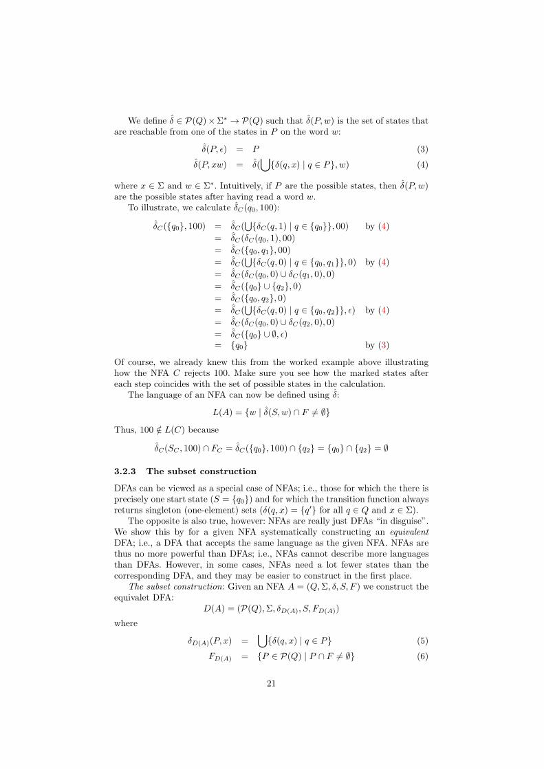
The subset construction: Given an NFA A = (Q,Σ, δ, S, F ) we construct theequivalet DFA:
D(A) = (P(Q),Σ, δD(A), S, FD(A))
where
δD(A)(P, x) =⋃
{δ(q, x) | q ∈ P} (5)
FD(A) = {P ∈ P(Q) | P ∩ F 6= ∅} (6)
21
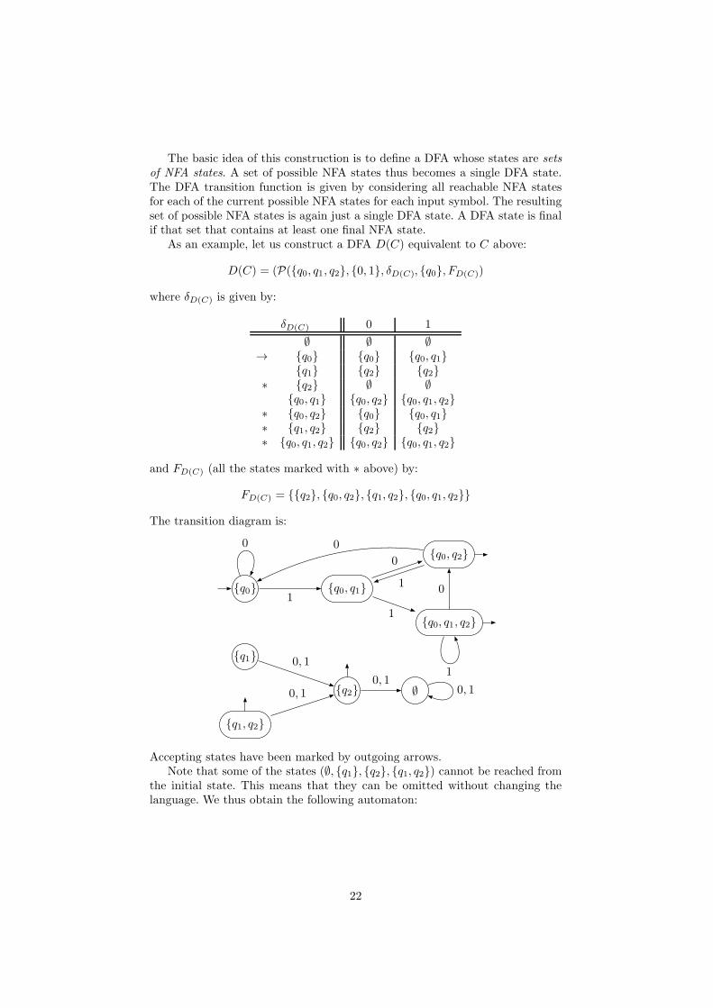
The basic idea of this construction is to define a DFA whose states are setsof NFA states. A set of possible NFA states thus becomes a single DFA state.The DFA transition function is given by considering all reachable NFA statesfor each of the current possible NFA states for each input symbol. The resultingset of possible NFA states is again just a single DFA state. A DFA state is finalif that set that contains at least one final NFA state.
As an example, let us construct a DFA D(C) equivalent to C above:
D(C) = (P({q0, q1, q2}, {0, 1}, δD(C), {q0}, FD(C))
where δD(C) is given by:
δD(C) 0 1
∅ ∅ ∅→ {q0} {q0} {q0, q1}
{q1} {q2} {q2}∗ {q2} ∅ ∅
{q0, q1} {q0, q2} {q0, q1, q2}∗ {q0, q2} {q0} {q0, q1}∗ {q1, q2} {q2} {q2}∗ {q0, q1, q2} {q0, q2} {q0, q1, q2}
and FD(C) (all the states marked with ∗ above) by:
FD(C) = {{q2}, {q0, q2}, {q1, q2}, {q0, q1, q2}}
The transition diagram is:
{q0} {q0, q1}
{q0, q2}
{q0, q1, q2}
{q1}
{q1, q2}
{q2} ∅
0
1
0
1
1
0
0
10, 1
0, 10, 1
0, 1
Accepting states have been marked by outgoing arrows.Note that some of the states (∅, {q1}, {q2}, {q1, q2}) cannot be reached from
the initial state. This means that they can be omitted without changing thelanguage. We thus obtain the following automaton:
22
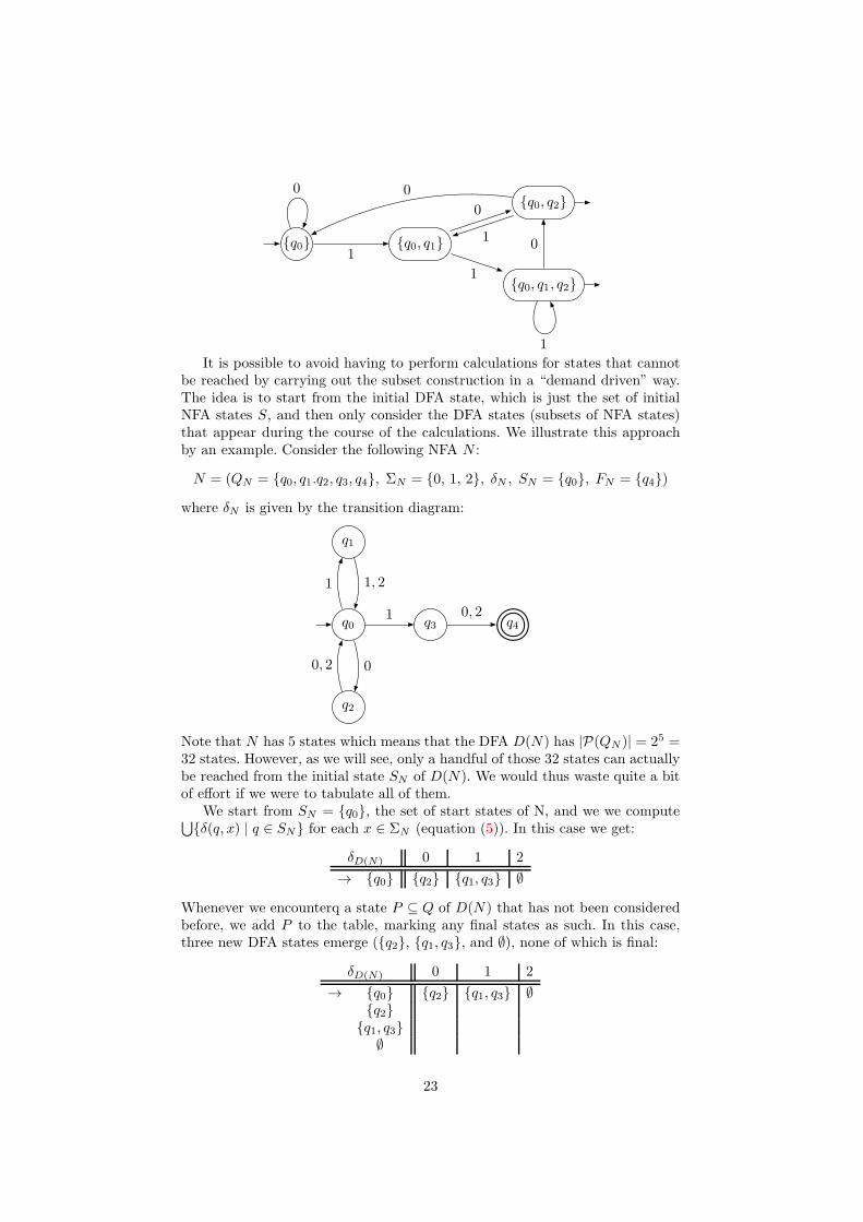
{q0} {q0, q1}
{q0, q2}
{q0, q1, q2}
0
1
0
1
1
0
0
1
It is possible to avoid having to perform calculations for states that cannotbe reached by carrying out the subset construction in a “demand driven” way.The idea is to start from the initial DFA state, which is just the set of initialNFA states S, and then only consider the DFA states (subsets of NFA states)that appear during the course of the calculations. We illustrate this approachby an example. Consider the following NFA N :
N = (QN = {q0, q1.q2, q3, q4}, ΣN = {0, 1, 2}, δN , SN = {q0}, FN = {q4})
where δN is given by the transition diagram:
q0
q1
q2
q3 q4
1 1, 2
00, 2
1 0, 2
Note that N has 5 states which means that the DFA D(N) has |P(QN )| = 25 =32 states. However, as we will see, only a handful of those 32 states can actuallybe reached from the initial state SN of D(N). We would thus waste quite a bitof effort if we were to tabulate all of them.
We start from SN = {q0}, the set of start states of N, and we we compute⋃
{δ(q, x) | q ∈ SN} for each x ∈ ΣN (equation (5)). In this case we get:
δD(N) 0 1 2
→ {q0} {q2} {q1, q3} ∅
Whenever we encounterq a state P ⊆ Q of D(N) that has not been consideredbefore, we add P to the table, marking any final states as such. In this case,three new DFA states emerge ({q2}, {q1, q3}, and ∅), none of which is final:
δD(N) 0 1 2
→ {q0} {q2} {q1, q3} ∅{q2}
{q1, q3}∅
23

We then proceed to tabulate δD(N) for each of the new states for each x ∈ Σ,adding any further new states to the table:
δD(N) 0 1 2
→ {q0} {q2} {q1, q3} ∅{q2} {q0} ∅ {q0}
{q1, q3} ∅ ∪ {q4} = {q4} {q0} ∪ ∅ = {q0} {q0} ∪ {q4} = {q0, q4}∅ ∅ ∅ ∅
Here, two new states emerge ({q4} and {q0, q4}), both final (because {q4}∩FN 6=∅ and {q0, q4} ∩ FN 6= ∅):
δD(N) 0 1 2
→ {q0} {q2} {q1, q3} ∅{q2} {q0} ∅ {q0}
{q1, q3} ∅ ∪ {q4} = {q4} {q0} ∪ ∅ = {q0} {q0} ∪ {q4} = {q0, q4}∅ ∅ ∅ ∅
∗ {q4}∗ {q0, q4}
This process is repeated until no new states emerges. Tabulating for the lasttwo new states reveals that no further states emerge in this case and we are thusdone, having only had to tabulate for 6 reachable out of the 32 DFA states:
δD(N) 0 1 2
→ {q0} {q2} {q1, q3} ∅{q2} {q0} ∅ {q0}
{q1, q3} ∅ ∪ {q4} = {q4} {q0} ∪ ∅ = {q0} {q0} ∪ {q4} = {q0, q4}∅ ∅ ∅ ∅
∗ {q4} ∅ ∅ ∅∗ {q0, q4} {q2} ∪ ∅ = {q2} {q1, q3} ∪ ∅ = {q1, q3} ∅ ∪ ∅ = ∅
After double checking that we have not forgotten to mark any final states,we can draw the transition diagram for D(N):
{q0}
{q2}
{q1, q3}
{q0, q4}
∅
{q4}
0
0, 2
1
1
2
1
0
0
2
2
1
0, 1, 2
0, 1, 2
Accepting states have been marked by outgoing arrows.
24
3.2.4 Correctness of the subset construction
We still have to convince ourselves that the subset construction actually works;i.e., that for a given NFA A it really is the case that L(A) = L(D(A)). Westart by proving the following lemma, which says that the extended transitionfunctions coincide:
Lemma 3.1δD(A)(P,w) = δA(P,w)
The result of both functions is a set of states of the NFA A: for the left-handside because the extended transition function on NFAs returns a set of states,and for the right-hand side because the states of D(A) are sets of states of A.
Proof. We show this by induction over the length of the word w, |w|.
|w| = 0 Then w = ǫ and we have
δD(A)(P, ǫ) = P by (1)
= δA(P, ǫ) by (3)
|w| = n+ 1 Then w = xv with |v| = n.
δD(A)(P, xv) = δD(A)(δD(A)(P, x), v) by (2)
= δA(δD(A)(P, x), v) ind.hyp.
= δA(⋃
{δA(q, x) | q ∈ P}, v) by (5)
= δA(P, xv) by (4)
�
We can now use the lemma to show
Theorem 3.2L(A) = L(D(A))
Proof.w ∈ L(A)
⇐⇒ Definition of L(A) for NFAs
δA(S,w) ∩ F 6= ∅⇐⇒ Lemma 3.1
δD(A)(S,w) ∩ F 6= ∅⇐⇒ Definition of FD(A)
δD(A)(S,w) ∈ FD(A)
⇐⇒ Definition of L(A) for DFAsw ∈ LD(A)
�
Corollary 3.3 NFAs and DFAs recognise the same class of languages.
Proof. We have noticed that DFAs are just a special case of NFAs. On theother hand the subset construction introduced above shows that for every NFAwe can find a DFA that recognises the same language. �
25

3.3 Exercises
Exercise 3.1
Let the alphabet Σ = {a, b} and consider the following DFA A:
A = (QA = {0, 1, 2, 3}, Σ, δA, q0 = 0, FA = {1, 2})
δA = {((0, a), 1), ((0, b), 2), ((1, a), 0), ((1, b), 3), ((2, a), 3), ((2, b), 0),
((3, a), 2), ((3, b), 1)}
(Here tuple notation is used to define the mapping of the transition functionδA; thus δA(0, a) = 1, δA(0, b) = 2, etc.) For the DFA A:
1. Draw its transition diagram.
2. Determine which of the following words belong to L(A):
1. ǫ
2. b
3. abaab
4. bababbba
3. Explicitly calculate δA(0, abba).
4. Describe the language that the automaton recognises in English.
Exercise 3.2
Construct a DFA B over Σ = {a, b, c, d} accepting all words where thenumber of a’s is a multiple of 3. E.g. abdaca ∈ L(B) (3 a’s), but ddaabaa /∈ L(B)(4 a’s, 4 is not a multiple of 3). Explain your construction. In particular, explainwhy you chose to have the number of states you did, and explain the purpose(or “meaning”) of each state.
Exercise 3.3
For the alphabet Σ = {0, 1, 2, 3}, construct a DFA C that precisely recognizesthe words for which the arithmetic sum of the constituent symbols is divisible by5. For example, ǫ ∈ L(C) (there are no symbols in the empty string, the sum isthus 0 which is divisible by 5), 0 ∈ L(C) (the sum is again 0), and 23131 ∈ L(C)(2 + 3 + 1 + 3 + 1 = 10 which is divisible by 5), but 133 /∈ L(C) (1 + 3 + 3 = 7which is not divisible by 5). Explain your construction.
26

Exercise 3.4
Consider the following NFA A over ΣA = {a, b, c}:
q0
q1 q2
q3 q4
a, b, c
a
b
c
a
c
b
1. Which of the following words are accepted by A and which are not?(a) ǫ(b) aaa(c) bbc(d) cbc(e) abcacb
2. Construct a DFA D(A) equivalent to A using the “subset construction”.Clearly show each step of your calculations in a transition table.Hint: Some of the 32 states (i.e., the 2|QA| = 25 = 32 possible subsets ofQA) that would arise by applying the subset construction blindly to Amay be unreachable. You can therefore adopt a strategy where you onlyconsider states reachable from the initial states, SA.
3. Draw the transition diagram for D(A), ignoring unreachable states.
Exercise 3.5
Consider the following NFA B over ΣB = {0, 1}:
q0
q1
q2
q3 q4
1 1
00
1 0
27

1. Construct a DFA D(B) equivalent to B using the “subset construction”and draw the transition diagram for D(B), ignoring unreachable states.Clearly show each step of your calculations, e.g. in a transition table.
2. Carry out a sanity check on your resulting DFA D(B) as follows.(a) Give two words over ΣB that are accepted by the NFA B and two
that are not. At least two of those should be four symbols long orlonger.
(b) Check that the DFAD(B) accepts the first two words and rejects theother two, exactly like the NFA B. Justify your answer by listing thesequence of states the DFA D(B) goes through for each word, andstating whether or not the last state of that sequence is accepting.
28

4 Regular Expressions
To recapitulate, given an alphabet Σ, a language is a set of words L ⊆ Σ∗. Sofar, we have described languages either using set theory (explicit enumerationor set comprehensions) or through finite automata. The key benefits of usingautomata is that they can describe infinite languages (unlike enumeration) andthat they directly give a mechanical way to determine language membership(unlike comprehensions). However, from an automaton, it is not usually imme-diately obvious what the language of that automaton is, and conversely, givena high-level description of a language, it is often not obvious if it is possible todescribe the language using a finite automaton.
This section introduces regular expressions : a concise and much more directway to describe languages. Moreover, a regular expression can mechanically betranslated into a finite automaton that accept precisely the language described.This opens up for many practical applications as languages can both be de-scribed and recognised with ease. In fact, the opposite is also true: given a finiteautomaton, it is possible to translate that into an equivalent regular expression.Finite automata and regular expressions are thus interconvertible, meaning thatthey describe the exact same class of languages: the regular languages or, ac-cording to the Chomsky hierarchy, type 3 languages (section 1.1).
One application of regular expressions is to define patterns in programssuch as grep. Given a regular expression and a sequence of text lines as input,grep returns those lines that match the regular expression, where matchingmeans that the line contains a substring that is in the language denoted by theregular expression. The syntax used by grep for regular expressions is slightlydifferent from the one used here, and grep further supports some convenientabbreviations. However, the underlying theory is exactly the same.
Other applications for regular expressions include defining the lexical syntaxof programming languages; i.e., what basic symbols, or tokens, such as identi-fiers, keywords, numeric literals look like, as well other lexical aspects such aswhite space and comments. The context-free syntax (see section 7) of a program-ming language is then defined in terms of the tokens; i.e., the tokens effectivelyconstitute the alphabet of the language.
In fact, regular expression matching has so many applications that manyprogramming languages provide support for this capability, either built-in orvia libraries. Examples include Perl, PHP, Python, and Java. In the past, someof those implementations were a bit naive as the regular expressions were notcompiled into finite automata. As a result, matching could be very slow, asexplained in the paper Regular Expression Matching Can Be Simple And Fast(but is slow in Java, Perl, PHP, Python, Ruby, ...) [Cox07]. This paper is avery good read, and once you have read these lecture notes up to and includingthe present section, you will be able to appreciate it fully.
4.1 What are regular expressions?
Given an alphabet Σ (e.g., Σ = {a, b, c, . . . , z}), the syntax (i.e., form) of regularexpressions over Σ is defined inductively as follows:
1. ∅ is a regular expression.
2. ǫ is a regular expression.
29
3. For each x ∈ Σ, x is a regular expression6.
4. If E and F are regular expressions then E + F is a regular expression.
5. If E and F are regular expressions then EF (juxtapositioning; just oneafter the other) is a regular expression.
6. If E is a regular expression then E∗ is a regular expression.
7. If E is a regular expression then (E) is a regular expression7.
These are all regular expressions.To illustrate, here are some examples of regular expressions:
• ǫ
• hallo
• hallo+ hello
• h(a+ e)llo
• a∗b∗
• (ǫ+ b)(ab)∗(ǫ+ a)
As in arithmetic, there are conventions for reading regular expressions:
• ∗ binds stronger than juxtapositioning and +. For example, ab∗ is readas a(b∗). Parentheses must be used to enforce the reading (ab)∗.
• Juxtapositioning binds stronger than +. For example, ab+ cd is read as(ab) + (cd). Parentheses must be used to enforce the reading a(b+ c)d.
4.2 The meaning of regular expressions
In the previous section, we defined the syntax of regular expressions, their form.We now proceed to define the semantics of regular expressions; i.e., what theymean, what language a regular expression denotes.
To answer this question, first recall the definition of concatenation of con-catenation of languages from section 2:
L1L2 = {uv |u ∈ L1 ∧ v ∈ L2}
We further recall the the Kleene star operation from the same section (2):
L∗ =
∞⋃
n=0
Ln
To each regular expression E over Σ we assign a language L(E) ⊆ Σ∗ as itsmeaning or semantics. We do this by induction over the definition of the syntax :
6 Note that the regular expression here is typeset in boldface, like a, to distinguish is fromthe corresponding symbol, like a, typeset in a type-writer font in this and the next section (andon occasion later on as well). Underlining is sometimes used as an alternative to boldface.
7 The parentheses have been typeset in boldface to emphasise that they are part of thesyntax of the regular expression.
30

1. L(∅) = ∅
2. L(ǫ) = {ǫ}
3. L(x) = {x} where x ∈ Σ.
4. L(E + F ) = L(E) ∪ L(F )
5. L(EF ) = L(E)L(F )
6. L(E∗) = L(E)∗
7. L((E)) = L(E)
Subtle points: In (1), the symbol ∅ is used both as a regular expression andas the empty set (empty language). Similarly, ǫ in (2) is used in two ways: asa regular expression and as the empty word. In (3), the regular expression istypeset in boldface to distinguish it from the corresponding symbol. In (6), the∗-operator is used both to construct a regular expression (part of the syntax)and as an operation on languages. In (7), the inner parentheses on the left-handside, typeset in boldface, are part of the syntax of regular expressions.
Let us now calculate the meaning of each of the regular expression examplesfrom the previous section; i.e., the language denoted in each case:
• ǫ:
By (2):
L(ǫ) = {ǫ}
• hallo:
Consider L(ha). By (3):
L(h) = {h}
L(a) = {a}
Hence, by (5) and language concatenation (section 2):
L(ha) = L(h)L(a)
= {uv | u ∈ L(h) ∧ vL(a)
= {uv | u ∈ {h} ∧ v ∈ {a}}
= {ha}
Continuing the same reasoning we obtain:
L(hallo) = {hallo}
• hallo+ hello:
From above we know L(hallo) = {hallo} and L(hello) = {hello}. By(4) we then get:
L(hallo+ hello) = {hallo} ∪ {hello}}
= {hallo, hello}
31
• h(a+ e)llo:
By (3) and (4) we know L(a+ e) = {a, e}. Thus, using (5) and languageconcatenation, we obtain:
L(h(a+ e)llo) = L(h)L(a+ e)L(llo)
= {uvw | u ∈ L(h) ∧ v ∈ L(a+ e) ∧ w ∈ L(llo)}
= {uvw | u ∈ {h} ∧ v ∈ {a, e} ∧w ∈ {llo}}
= {hallo, hello}
• a∗b∗:
By (6):
L(a∗) = L(a)∗
= {a}∗
=
∞⋃
n=0
{a}n
=
∞⋃
n=0
{w1w1 . . . wn | 1 ≤ i ≤ n, wi ∈ {a}}
=
∞⋃
n=0
{an}
= {an | n ∈ N}
Using (5) and language concatenation, this allows us to conclude:
L(a∗b∗) = L(a∗)L(b∗)
= {uv | u ∈ L(a∗) ∧ v ∈ L(b∗)}
= {uv | u ∈ {am | m ∈ N} ∧ v ∈ {bn | n ∈ N}}
= {ambn | m,n ∈ N}
That is, L(a∗b∗) is the set of all words that start with a (possibly empty)sequence of a’s, followed by a (possibly empty) sequence of b’s.
• (ǫ+ b)(ab)∗(ǫ+ a):
Let us analyse the parts:
L(ǫ+ b) = {ǫ, b}
L((ab)∗) = {(ab)n | n ∈ N}
L(ǫ+ a) = {ǫ, a}
Thus, we have:
L((ǫ+ b)(ab)∗(ǫ + a)) = {u(ab)nv | u ∈ {ǫ, b} ∧ n ∈ N ∧ v ∈ {ǫ, a}}
In English: L((ǫ+b)(ab)∗(ǫ+a)) is the set of (possibly empty) sequencesof alternating a’s and b’s.
32
4.3 Algebraic laws
The semantics of regular expressions not only allows us to find out the meaningof specific regular expressions, but also allows us to prove useful laws about reg-ular expression in general. Let us illustrate by proving the following distributivelaw for regular expressions:
E(F +G) = EF + EG
Note that E, F , G are variables standing for some specific but arbitrary regularexpressions, and that = here is semantic (as opposed to syntactic) equality. Thatis, what we need to prove is that a regular expression of the form E(F +G) andone of the form EF +EG always have the same meaning, i.e., denote the samelanguage.
We thus start from L(E(F + G)) and show step by step that this is equalto L(EF +EG) without making any assumptions about the constituent regularexpressions E, F , and G, other than that their semantics is given by L(E) etc.
L(E(F +G))= { Semantics of r.e. (concat.) }
L(E)L(E + F )= { Semantics of r.e. (+) }
L(E)(L(F ) ∪ L(G))= { Def. concat. of languages }
{w1w2 | w1 ∈ L(E) ∧ w2 ∈ (L(F ) ∪ L(G))}= { Def. set union }
{w1w2 | w1 ∈ L(E) ∧ w2 ∈ {w | w ∈ L(F ) ∨ w ∈ L(G)}}= { Duality between sets and predicates }
{w1w2 | w1 ∈ L(E) ∧ (w2 ∈ L(F ) ∨w2 ∈ L(G))}= { Conjunction (∧) distributes over disjunction (∨) }
{w1w2 | (w1 ∈ L(E) ∧ w2 ∈ L(F )) ∨ (w1 ∈ L(E) ∧w2 ∈ L(G))}= { Def. set union }
{w1w2 | (w1 ∈ L(E) ∧ w2 ∈ L(F ))} ∪ {w1w2 | (w1 ∈ L(E) ∧ w2 ∈ L(G))}= { Def. concat. languages (twice) }
L(E)L(F ) ∪ L(E)L(G)= { Semantics of r.e. (conacat., twice) }
L(EF ) ∪ L(EG)= { Semantics of r.e. (+) }
L(EF + EG)
Other laws for regular expressions can be proved similarly, although induc-tion is sometimes needed. As an exercise, prove (some of) the following:
ǫE = E
Eǫ = E
∅E = ∅
E∅ = ∅
E + (F +G) = (E + F ) +G
E(FG) = (EF )G
(E∗)∗ = E∗
ǫ + EE∗ = E∗
33

4.4 Translating regular expressions into NFAs
Theorem 4.1 A regular expression E can be translated into an equivalent NFAN(E) such that L(N(E)) = L(E).
We refer to this translation as the “Graphical Construction”. It is a variationof the standard way of translating regular expressions into NFAs known asThompson’s construction8.
Proof. The proof is by induction on the syntax of regular expressions:
1. N(∅):
which will reject everything (there are no final states). Thus:
L(N(∅)) = ∅
= L(∅)
2. N(ǫ):
This automaton accepts the empty word but rejects everything else. Thus
L(N(ǫ)) = {ǫ}
= L(ǫ)
3. N(x):
This automaton only accepts the word x. Thus:
L(N(x)) = {x}
= L(x)
4. N(E + F ): We merge the diagrams for N(E) and N(F ) into one:
8https://en.wikipedia.org/wiki/Thompson%27s construction
34

Intuitively, the NFAs for the subexpressions E and F are placed side byside. Thus if either of the NFA accepts a word, the combined NFA acceptsthis word. However, we have to ensure that the states of the constituentNFAs do not get confused with each other. We therefore have to use thedisjoint union, defined as follows:
A ⊎B = {(0, a) | a ∈ A} ∪ {(1, b) | b ∈ B}
That is, each element of the disjoint union is “tagged” with an indexthat shows from which of the two sets it originated. Thus the elementsof the constituent sets will remain distinct. The transition function of thecombined NFA also has to be defined to work on tagged states.
Thus, given the NFAs for the subexpressions E and F :
N(E) = (QE ,Σ, δE , SE, FE)
N(F ) = (QF ,Σ, δF , SF , FF )
we construct the combined NFA for the regular expression E + F :
N(E + F ) = (QE+F ,Σ, δE+F , SE+F , FE+F )
where
QE+F = QE ⊎QF
δE+F ((0, q), x) = {(0, q′) | q′ ∈ δE(q, x)}
δE+F ((1, q), x) = {(1, q′) | q′ ∈ δF (q, x)}
SE+F = SE ⊎ SF
FE+F = FE ⊎ FF
It remains to prove L(N(E + F )) = L(E + F ). We first observe that
L(N(E + F )) = L(N(E)) ∪ L(N(F ))
because the initial states SE+F of the combined NFA is the (disjoint) unionof the initial states of the constituent NFAs, and because the combinedNFA accepts a word whenever one of the constituent NFAs does.
The proof then proceeds by induction; that is, we assume that the trans-lation is correct for the subexpressions:
L(N(E)) = L(E)
L(N(F )) = L(F )
Thus:
L(N(E + F )) = L(N(E)) ∪ L(N(F )) Above= L(E) ∪ L(F ) Induction hypothesis= L(E + F ) By (4)
This is what is meant by induction over the syntax of regular expressions.
35
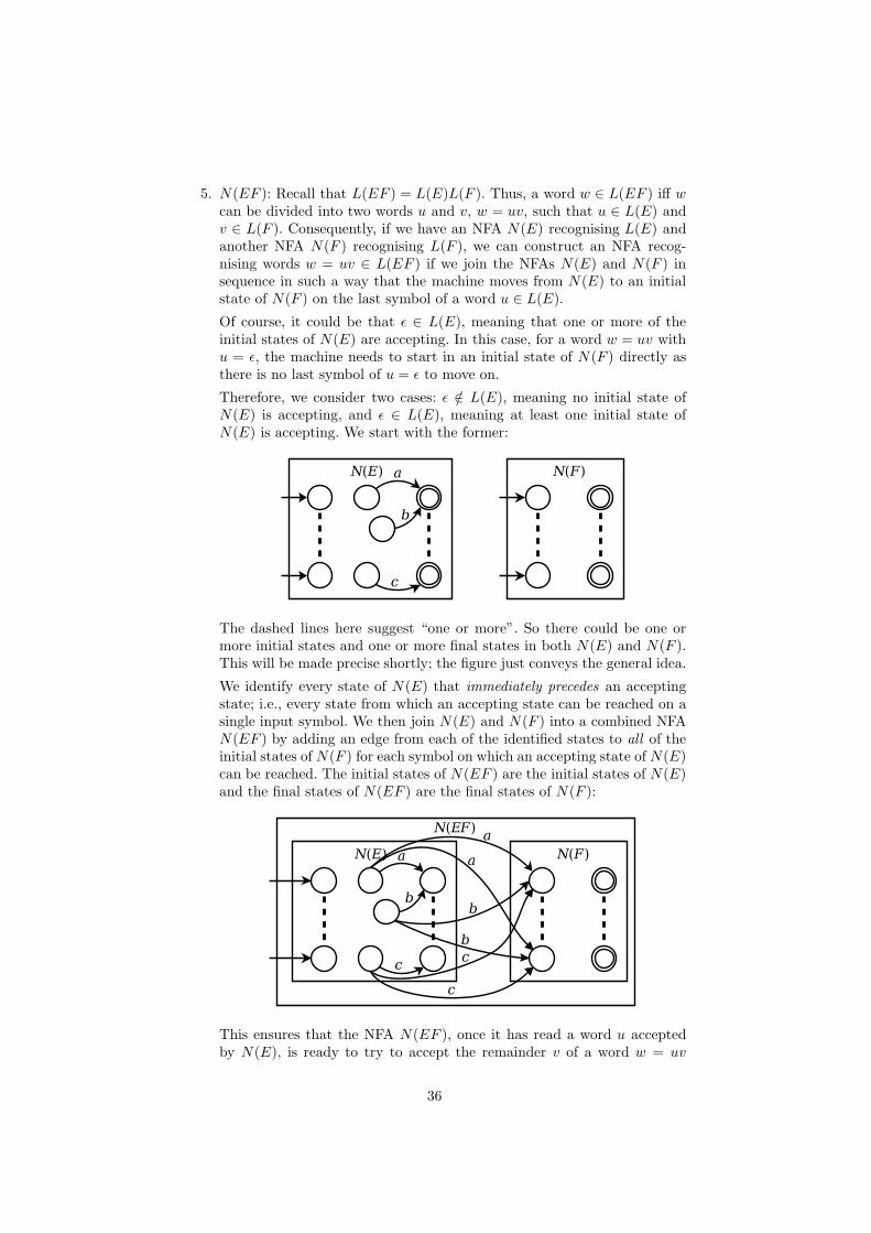
5. N(EF ): Recall that L(EF ) = L(E)L(F ). Thus, a word w ∈ L(EF ) iff wcan be divided into two words u and v, w = uv, such that u ∈ L(E) andv ∈ L(F ). Consequently, if we have an NFA N(E) recognising L(E) andanother NFA N(F ) recognising L(F ), we can construct an NFA recog-nising words w = uv ∈ L(EF ) if we join the NFAs N(E) and N(F ) insequence in such a way that the machine moves from N(E) to an initialstate of N(F ) on the last symbol of a word u ∈ L(E).
Of course, it could be that ǫ ∈ L(E), meaning that one or more of theinitial states of N(E) are accepting. In this case, for a word w = uv withu = ǫ, the machine needs to start in an initial state of N(F ) directly asthere is no last symbol of u = ǫ to move on.
Therefore, we consider two cases: ǫ /∈ L(E), meaning no initial state ofN(E) is accepting, and ǫ ∈ L(E), meaning at least one initial state ofN(E) is accepting. We start with the former:
The dashed lines here suggest “one or more”. So there could be one ormore initial states and one or more final states in both N(E) and N(F ).This will be made precise shortly; the figure just conveys the general idea.
We identify every state of N(E) that immediately precedes an acceptingstate; i.e., every state from which an accepting state can be reached on asingle input symbol. We then join N(E) and N(F ) into a combined NFAN(EF ) by adding an edge from each of the identified states to all of theinitial states of N(F ) for each symbol on which an accepting state of N(E)can be reached. The initial states of N(EF ) are the initial states of N(E)and the final states of N(EF ) are the final states of N(F ):
This ensures that the NFA N(EF ), once it has read a word u acceptedby N(E), is ready to try to accept the remainder v of a word w = uv
36
by effectively passing v to N(F ), allowing the latter to try to accept theremaining part v of w from any of its initial states.
We now formalise this construction. The set of states of the combinedNFA N(EF ) is again given by the disjoint union of the states of N(E)and N(F ) to avoid confusion, and the transition function δEF as well asthe initial states SEF and final states FEF are defined accordingly.
Thus, given the NFAs for the subexpressions E and F :
N(E) = (QE ,Σ, δE , SE, FE)
N(F ) = (QF ,Σ, δF , SF , FF )
we construct the combined NFA for the regular expression EF :
N(EF ) = (QEF ,Σ, δEF , SEF , FEF )
where
QEF = QE ⊎QF
δEF ((0, q), x) = {(0, q′) | q′ ∈ δE(q, x)}
∪ {(1, q′) | δE(q, x) ∩ FE 6= ∅ ∧ q′ ∈ SF }
δEF ((1, q), x) = {(1, q′) | q′ ∈ δF (q, x)}
SEF = {(0, q) | q ∈ SE}
FEF = {(1, q) | q ∈ FF }
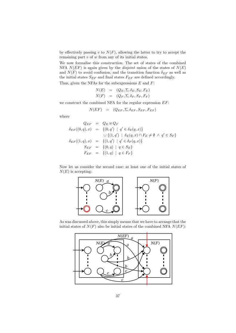
Now let us consider the second case: at least one of the initial states ofN(E) is accepting:
As was discussed above, this simply means that we have to arrange that theinitial states of N(F ) also be initial states of the combined NFA N(EF ):
37

We thus refine the formal definition of the initial states of N(EF ) toaccount for this, yielding a definition that covers both cases:
SEF = {(0, q) | q ∈ SE}
∪ {(1, q) | SE ∩ FE 6= ∅ ∧ q ∈ SF }
It remains to prove L(N(EF )) = L(EF ). From the construction above, itis clear that
L(N(EF )) = {uv | u ∈ L(N(E)) ∧ v ∈ L(N(F ))}
The proof again proceeds by induction; that is, we assume that the trans-lation is correct for the subexpressions:
L(N(E)) = L(E)
L(N(F )) = L(F )
Thus:
L(N(EF )) = {uv | u ∈ L(N(E)) ∧ v ∈ L(N(F ))} Above= {uv | u ∈ L(E) ∧ v ∈ L(F )} Ind. hyp.= L(E)L(F ) Lang. concat.= L(EF ) By (5)
6. N(E∗): Recall that L(E∗) = L(E)∗. Thus, a word w ∈ L(E∗) iff w canbe divided into a sequence of n ∈ N words ui, w = u1u2 . . . un, suchthat ∀i ∈ [1, n] . ui ∈ L(E). Consequently, if we have an NFA N(E)recognising L(E), we can construct an NFA recognising words w ∈ L(E∗)by connecting 0 or more NFAs N(E) in sequence in a similar way to whatwe did for the case N(EF ) above:
Here we use the * to informally suggest sequential composition of 0 ormore NFAs.
However, we need to construct a single NFA, and there is no upper boundon the number of NFAs N(E) that we need to connect in sequence. Weresolve this by taking a single NFA N(E) and construct and NFA forN(E∗) by making it loop back to all of its own initial states from eachstate that immediately precedes an accepting state. As we also need toallow for iteration 0 times, we further have to add one extra state that isboth initial and final thus accepting ǫ:
38
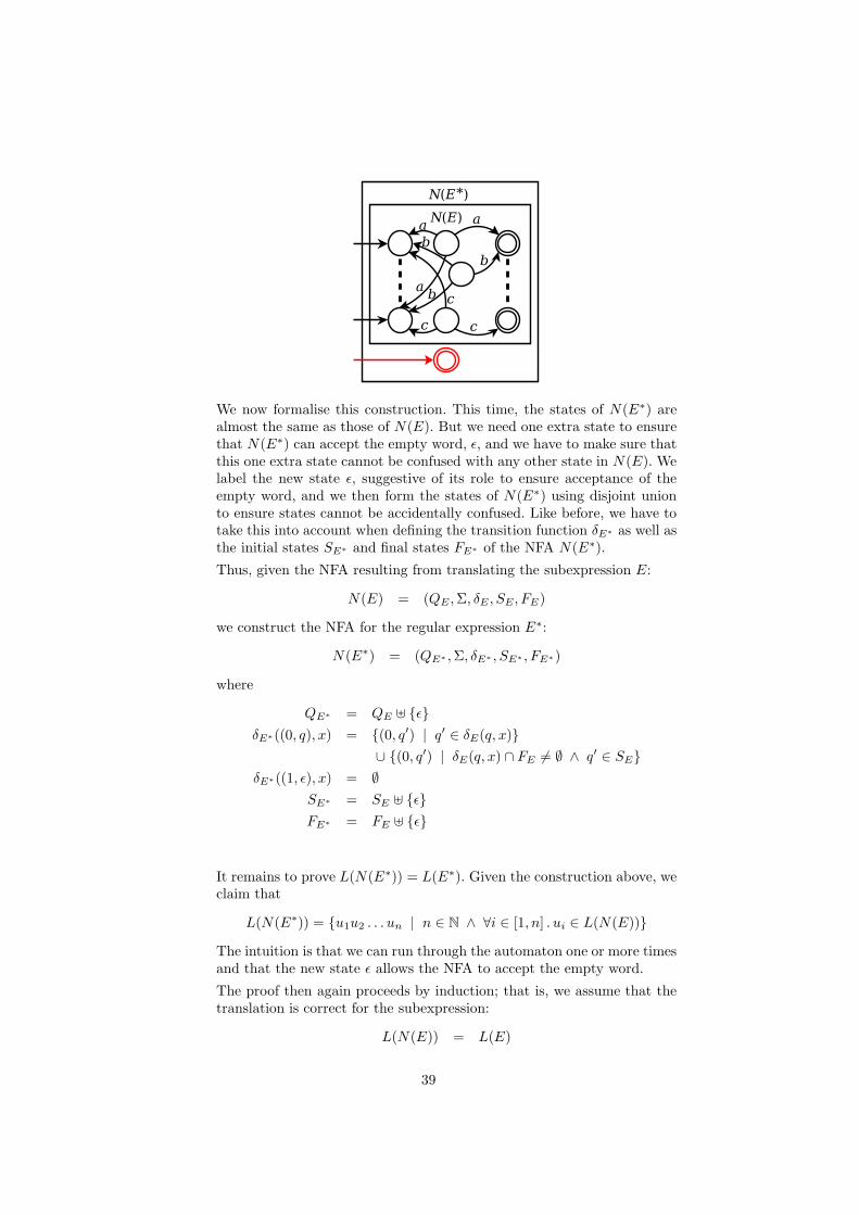
We now formalise this construction. This time, the states of N(E∗) arealmost the same as those of N(E). But we need one extra state to ensurethat N(E∗) can accept the empty word, ǫ, and we have to make sure thatthis one extra state cannot be confused with any other state in N(E). Welabel the new state ǫ, suggestive of its role to ensure acceptance of theempty word, and we then form the states of N(E∗) using disjoint unionto ensure states cannot be accidentally confused. Like before, we have totake this into account when defining the transition function δE∗ as well asthe initial states SE∗ and final states FE∗ of the NFA N(E∗).
Thus, given the NFA resulting from translating the subexpression E:
N(E) = (QE ,Σ, δE , SE, FE)
we construct the NFA for the regular expression E∗:
N(E∗) = (QE∗ ,Σ, δE∗ , SE∗ , FE∗)
where
QE∗ = QE ⊎ {ǫ}
δE∗((0, q), x) = {(0, q′) | q′ ∈ δE(q, x)}
∪ {(0, q′) | δE(q, x) ∩ FE 6= ∅ ∧ q′ ∈ SE}
δE∗((1, ǫ), x) = ∅
SE∗ = SE ⊎ {ǫ}
FE∗ = FE ⊎ {ǫ}
It remains to prove L(N(E∗)) = L(E∗). Given the construction above, weclaim that
L(N(E∗)) = {u1u2 . . . un | n ∈ N ∧ ∀i ∈ [1, n] . ui ∈ L(N(E))}
The intuition is that we can run through the automaton one or more timesand that the new state ǫ allows the NFA to accept the empty word.
The proof then again proceeds by induction; that is, we assume that thetranslation is correct for the subexpression:
L(N(E)) = L(E)
39

Thus:
L(N(E∗)) = { u1u2 . . . un Above| n ∈ N ∧ ∀i ∈ [1, n] . ui ∈ L(N(E)) }
= { u1u2 . . . un Ind. hyp.| n ∈ N ∧ ∀i ∈ [1, n] . ui ∈ L(E) }
=⋃∞
n=0 L(E)n Lang. concat.= L(E)∗ Def. Kleene star= L(E∗) By (6)
7. N((E)) = N(E): Parentheses are just used for grouping and does notchange anyting.
We need to prove L(N((E))) = L((E)). The proof is again by induction,so we assume L(N(E)) = L(E) and then we proceed as follows:
L(N((E))) = L(N(E)) By construction= L(E) Induction hypothesis= L((E)) By (7)
�
It is worth pausing briefly to reflect on what we just have accomplished.In effect, we have implemented a compiler that translates regular expressionsinto NFAs, and we have proved it correct; that is, the translation preserves themeaning (here, the described language), which after all is what we generallyexpect of an accurate translation. Of course, it is a very simple compiler. Yet,in essence, it reflects how real tools that handle regular expressions work; forexample, scanner (or lexer) generators such as Flex, Ragel, or Alex9. Moreover,while proving the correctness of compilers for typical programming languages isvastly more complicated than what we have seen here, there are methodologicalsimilarities, such as proof by induction over the structure of the language.
Let us illustrate how to apply the Graphical Construction. As a first example,we construct N(a∗b∗). We start with the innermost subexpressions and thenjoin the NFAs together step by step. The states are named according to howthey will be named in the final NFA to make it easier to follow the derivation.It is fine to leave states unnamed until the end, and that is what normally isdone. We begin with the NFA for a:
0 4a
The NFA for a∗ is obtained by adding a loop on a from state 0 to itself asthis state precedes a final state and is the only initial state, and by adding theextra state for accepting ǫ:
9 https://en.wikipedia.org/wiki/Lexical analysis
40

0 4
a
a
5
The NFA for b∗ is constructed in the same way:
1 2
b
b
3
Now we have to join these two NFAs in sequence:
0 4
a
a
5
1 2
b
b
3
We have to pay extra attention because the automaton for the subexpressiona∗ contains a state that is both initial and final, namely state 5, resulting in“extra” initial states when composing that automaton with the automaton forthe subexpression b∗:
0 4
a
a
5
1 2
b
b
3
a
a
The states 4 and 5 have manifestly become “dead ends”: there is no way toreach a final state from either. For NFAs, such dead ends can simply be removed
41

(along with associated edges) without changing the accepted language. If we dothat, we obtain:
0
a1 2
b
b
3
a
a
You may have noted that, though correct, this NFA is unnecessary com-plicated. For example, the following NFA also accepts N(a∗b∗), but has fewerstates:
0 1
a
b
b
This is typical: the translation of regular expressions into NFAs does generallynot yield the simplest possible automata.
If we are interested in obtaining the smallest possible machine, one approachis to first convert the resulting NFA into a DFA using the subset constructionof section 3.2.3 and then minimize this DFA as explained in section 5. If we dothis for the four-state NFA above, we obtain the following DFA:
0 1 2
a
b
b
a
a, b
As it happens, just applying the subset construction to the four-state NFA yieldsthis DFA directly10: it is already minimal. Try it! It is quick and a good exercise.
Let us do one more, somewhat larger, example: constructing an NFA for((a + ǫ)(b + c))∗. We again start with the innermost subexpressions and thenjoin the NFAs together step by step. We have to (again) pay extra attentionbecause the automaton for the subexpression (a + ǫ) contains a state that isboth initial and final, resulting in “extra” initial states when composing thatautomaton with the automaton for the subexpression (b + c). Also, it makessense to eliminate dead ends as soon as they occur, here before closing the loopdue to the top-level Kleene star. The states are named according to how theywill be named in the final NFA to make it easier to follow the derivation, butcould be left unnamed until the end if you prefer.
First, an NFA for a+ ǫ:
10 Or one isomorphic to it: the states will probably be named differently.
42

0 6a
7
NFA for b+ c
1 2
3 4
b
c
Join the above two NFAs to obtain an NFA for (a+ ǫ)(b+ c):
0 6
7
1 2
3 4
a
a
a
b
c
Note that both state 1 and 3 remain initial states states because the left au-tomaton has an initial state that is also accepting, meaning we need to be ableto get to the start states of the right automaton without consuming any input.
States 6 and 7 have now manifestly become dead ends because there is no wayto reach an accepting state from either. Let us remove them and all associatededges:
0
1 2
3 4
a
a
b
c
The last step is to carry out the construction corresponding to the ∗-operator.States 1 and 3 both immediately precede a final state, and we should thus addcorresponding transition edges from those back to all initial states. There arethree initial states, 0, 1, and 3. Thus we need an edge labelled b from 1 to eachof 0, 1, and 3 (i.e., a loop back to itself on b) and and an edge labelled c from 3to each of 0, 1, and 3 (i.e., a loop back to itself on c). Additionally, we must notforget to add an extra initial state which is also final (here state 5) to ensurethe NFA accepts ǫ.
43
0
1 2
3 4
5
a
ab
b
c
c
b
b
c
c
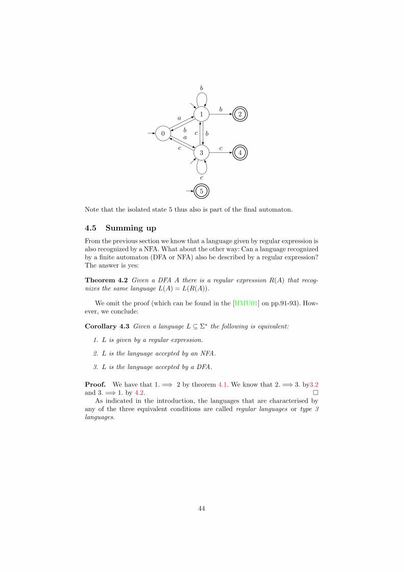
Note that the isolated state 5 thus also is part of the final automaton.
4.5 Summing up
From the previous section we know that a language given by regular expression isalso recognized by a NFA. What about the other way: Can a language recognizedby a finite automaton (DFA or NFA) also be described by a regular expression?The answer is yes:
Theorem 4.2 Given a DFA A there is a regular expression R(A) that recog-nizes the same language L(A) = L(R(A)).
We omit the proof (which can be found in the [HMU01] on pp.91-93). How-ever, we conclude:
Corollary 4.3 Given a language L ⊆ Σ∗ the following is equivalent:
1. L is given by a regular expression.
2. L is the language accepted by an NFA.
3. L is the language accepted by a DFA.
Proof. We have that 1. =⇒ 2 by theorem 4.1. We know that 2. =⇒ 3. by3.2and 3. =⇒ 1. by 4.2. �
As indicated in the introduction, the languages that are characterised byany of the three equivalent conditions are called regular languages or type 3languages.
44

4.6 Exercises
Exercise 4.1
Give regular expressions defining the following languages over the alphabet Σ ={a, b, c}:
1. All words that contain exactly one a.
2. All words that contain at least two bs.
3. All words that contain at most two cs.
4. All words such that all b’s appear before all c’s.
5. All words that contain exactly one b and one c (but any number of a’s).
6. All words such that the number of a’s plus the number of b’s is odd.
Exercise 4.2
Using the formal definition of the meaning of regular expressions, computethe set denoted by the regular expression
(aa+ ǫb∗∅)(b+ c)
simplifying as far as possible. Provide a step-by-step account.
Exercise 4.3
Systematically construct an NFA for the regular expression
(a(∅∗ + b))∗(c+ ǫ+ ∅)
by following the graphical construction from the lecture notes. Make sure it isclear how you undertake the construction by showing the major steps. Eliminate“dead ends” (states from which no final state can be reached) when they appear.The states in the final NFA should be named, but as long as it is clear whatyou are doing, you can leave the states of intermediate NFAs unnamed.
45

5 Minimization of Finite Automata
As we saw when translating regular expressions into NFAs, the resulting au-tomaton is not necessarily the smallest possible one. Similarly, when employingthe subset construction to translate an NFA into a DFA, the result is not alwaysthe smallest possible DFA. It is often desirable to make automatons as small aspossible. For example, if we wish to implement an automaton, the implementa-tion will be more efficient the smaller the automaton is.
Given an automaton, the question, then, is how to construct an equivalentbut smaller automaton. Recall that two automatons are equivalent of they ac-cept the same language. In the following we will study a method for minimizingDFAs: the table-filling algorithm.
Another interesting question is if there, in general, is one unique automatonthat is the smallest equivalent one, or if there can be many distinct equivalentautomatons, none of which can be made any smaller. It turns out the answer isthat the minimal equivalent DFA is unique up to naming of the states. This, inturn, means that we have obtained a mechanical decision procedure for deter-mining whether two regular languages are equal: simply convert their respectiverepresentation (be it a DFA, an NFA, or a regular expression) to DFAs andminimize them. Since the minimal DFAs are unique, the languages are equal ifand only if the minimal DFAs are equal.
5.1 The table-filling algorithm
For a DFA (Q,Σ, δ, q0, F ), p, q ∈ Q are equivalent states if and only if, for all
w ∈ Σ∗, δ(p, w) ∈ F ⇔ δ(q, w) ∈ F . If two states are not equivalent, then theyare distinguishable.
Consider the following DFA, where Σ = {a, b}, Q = {0, 1, 2, 3, 4, 5}, F ={2, 3}:
0 1 2
34
5
a
b
a
b
a, b
a
b
a
b
ab
The states 1 and 2 are distinguishable on ǫ since δ(1, ǫ) = 1 /∈ F while δ(2, ǫ) =
2 ∈ F . Similarly, 0 and 1 are distinguishable on e.g. b since δ(0, b) = 4 /∈ F
while δ(1, b) = 3 ∈ F . On the other hand, in this case, we can easily see that 4and 5 are not distinguishable on any word since it is not possible to reach anyaccepting (final) state from either 4 or 5.
The Table-Filling Algorithm recursively constructs the set of distinguish-able pairs of states for a DFA. When all distinguishable state pairs have been
46
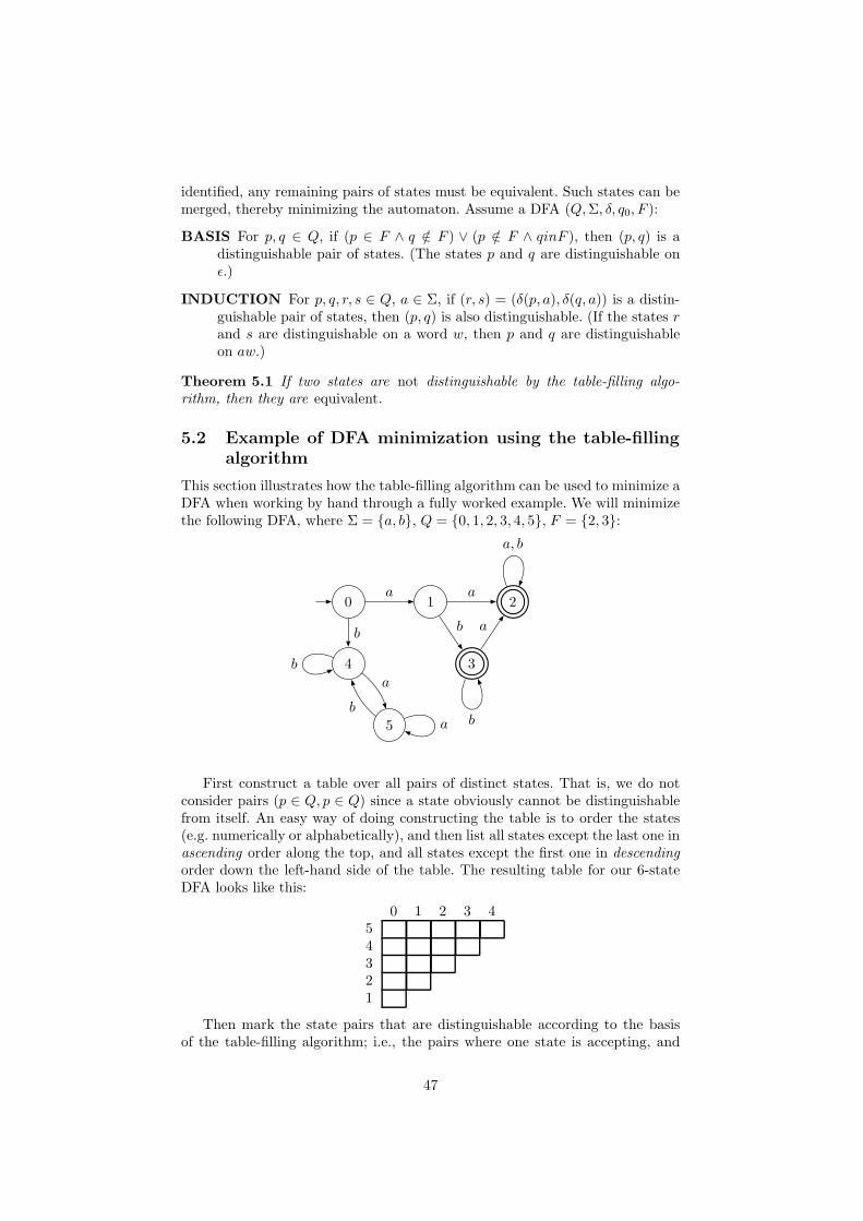
identified, any remaining pairs of states must be equivalent. Such states can bemerged, thereby minimizing the automaton. Assume a DFA (Q,Σ, δ, q0, F ):
BASIS For p, q ∈ Q, if (p ∈ F ∧ q /∈ F ) ∨ (p /∈ F ∧ qinF ), then (p, q) is adistinguishable pair of states. (The states p and q are distinguishable onǫ.)
INDUCTION For p, q, r, s ∈ Q, a ∈ Σ, if (r, s) = (δ(p, a), δ(q, a)) is a distin-guishable pair of states, then (p, q) is also distinguishable. (If the states rand s are distinguishable on a word w, then p and q are distinguishableon aw.)
Theorem 5.1 If two states are not distinguishable by the table-filling algo-rithm, then they are equivalent.
5.2 Example of DFA minimization using the table-filling
algorithm
This section illustrates how the table-filling algorithm can be used to minimize aDFA when working by hand through a fully worked example. We will minimizethe following DFA, where Σ = {a, b}, Q = {0, 1, 2, 3, 4, 5}, F = {2, 3}:
0 1 2
34
5
a
b
a
b
a, b
a
b
a
b
ab
First construct a table over all pairs of distinct states. That is, we do notconsider pairs (p ∈ Q, p ∈ Q) since a state obviously cannot be distinguishablefrom itself. An easy way of doing constructing the table is to order the states(e.g. numerically or alphabetically), and then list all states except the last one inascending order along the top, and all states except the first one in descendingorder down the left-hand side of the table. The resulting table for our 6-stateDFA looks like this:
0 1 2 3 454321
Then mark the state pairs that are distinguishable according to the basisof the table-filling algorithm; i.e., the pairs where one state is accepting, and
47
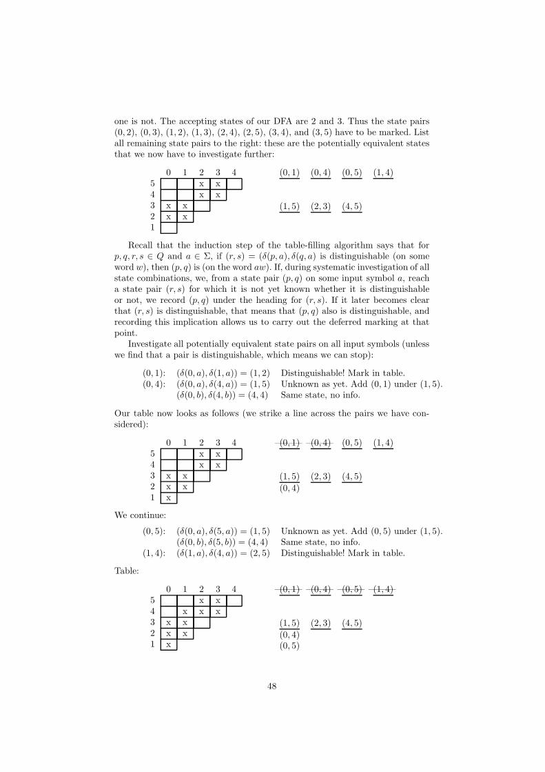
one is not. The accepting states of our DFA are 2 and 3. Thus the state pairs(0, 2), (0, 3), (1, 2), (1, 3), (2, 4), (2, 5), (3, 4), and (3, 5) have to be marked. Listall remaining state pairs to the right: these are the potentially equivalent statesthat we now have to investigate further:
0 1 2 3 45 x x4 x x3 x x2 x x1
(0, 1) (0, 4) (0, 5) (1, 4)
(1, 5) (2, 3) (4, 5)
Recall that the induction step of the table-filling algorithm says that forp, q, r, s ∈ Q and a ∈ Σ, if (r, s) = (δ(p, a), δ(q, a) is distinguishable (on someword w), then (p, q) is (on the word aw). If, during systematic investigation of allstate combinations, we, from a state pair (p, q) on some input symbol a, reacha state pair (r, s) for which it is not yet known whether it is distinguishableor not, we record (p, q) under the heading for (r, s). If it later becomes clearthat (r, s) is distinguishable, that means that (p, q) also is distinguishable, andrecording this implication allows us to carry out the deferred marking at thatpoint.
Investigate all potentially equivalent state pairs on all input symbols (unlesswe find that a pair is distinguishable, which means we can stop):
(0, 1): (δ(0, a), δ(1, a)) = (1, 2) Distinguishable! Mark in table.(0, 4): (δ(0, a), δ(4, a)) = (1, 5) Unknown as yet. Add (0, 1) under (1, 5).
(δ(0, b), δ(4, b)) = (4, 4) Same state, no info.
Our table now looks as follows (we strike a line across the pairs we have con-sidered):
0 1 2 3 45 x x4 x x3 x x2 x x1 x
———(0, 1) ———(0, 4) (0, 5) (1, 4)
(1, 5) (2, 3) (4, 5)
(0, 4)
We continue:
(0, 5): (δ(0, a), δ(5, a)) = (1, 5) Unknown as yet. Add (0, 5) under (1, 5).(δ(0, b), δ(5, b)) = (4, 4) Same state, no info.
(1, 4): (δ(1, a), δ(4, a)) = (2, 5) Distinguishable! Mark in table.
Table:
0 1 2 3 45 x x4 x x x3 x x2 x x1 x
———(0, 1) ———(0, 4) ———(0, 5) ———(1, 4)
(1, 5) (2, 3) (4, 5)
(0, 4)(0, 5)
48

Now we have come to the state pair (1, 5). If we can determine that (1, 5) isa distinguishable pair, then we also know that the pairs (0, 4) and (0, 5) aredistinguishable:
(1, 5): (δ(1, a), δ(5, a)) = (2, 5) Distinguishable!
Thus we should mark (1, 5) along with and (0, 4) and (0, 5):
0 1 2 3 45 x x x x4 x x x x3 x x2 x x1 x
———(0, 1) ———(0, 4) ———(0, 5) ———(1, 4)
———(1, 5) (2, 3) (4, 5)
———(0, 4)———(0, 5)
It remains to check the pairs (2, 3) and (4, 5):
(2, 3): (δ(2, a), δ(3, a)) = (2, 2) Same state, no info.(δ(2, b), δ(3, b)) = (2, 3) No point in adding (2, 3) below (2, 3).
(4, 5): (δ(4, a), δ(5, a)) = (5, 5) Same state, no info.(δ(4, b), δ(5, b)) = (4, 4) Same state, no info.
We have now systematically checked all potentially equivalent state pairs.Two pairs remain unmarked; i.e., we have not been able to show that they aredistinguishable: (2, 3) and (4, 5). We can therefore conclude that these statesare pairwise equivalent: 2 ≡ 3 and 4 ≡ 5. We thus proceed to merge these statesby, informally, placing them “on top” of each other and “dragging along” theedges. The result is the following minimal DFA (where the merged states havebeen given the names 2 and 4):
0 1 2
4
a
b
a, b
a, b
a, b
49
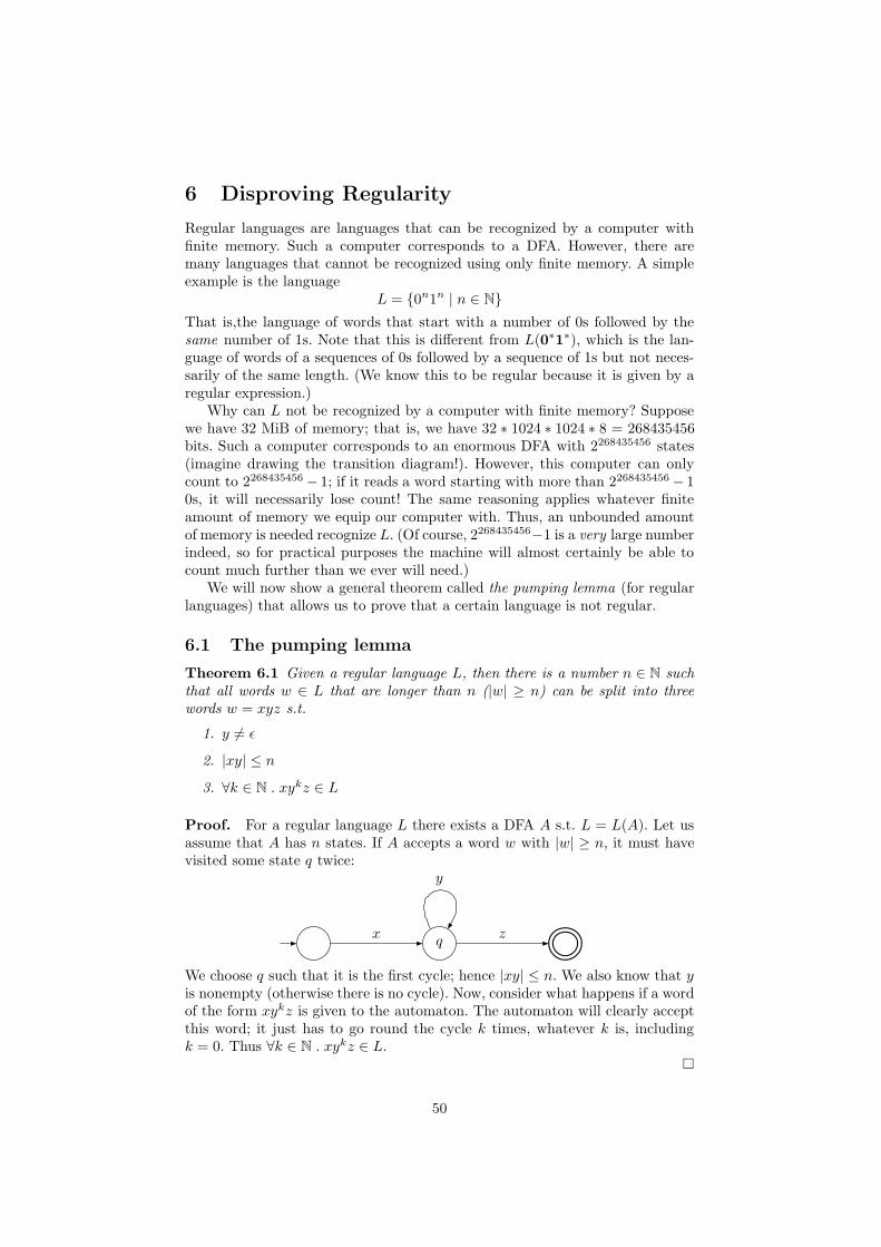
6 Disproving Regularity
Regular languages are languages that can be recognized by a computer withfinite memory. Such a computer corresponds to a DFA. However, there aremany languages that cannot be recognized using only finite memory. A simpleexample is the language
L = {0n1n | n ∈ N}
That is,the language of words that start with a number of 0s followed by thesame number of 1s. Note that this is different from L(0∗1∗), which is the lan-guage of words of a sequences of 0s followed by a sequence of 1s but not neces-sarily of the same length. (We know this to be regular because it is given by aregular expression.)
Why can L not be recognized by a computer with finite memory? Supposewe have 32 MiB of memory; that is, we have 32 ∗ 1024 ∗ 1024 ∗ 8 = 268435456bits. Such a computer corresponds to an enormous DFA with 2268435456 states(imagine drawing the transition diagram!). However, this computer can onlycount to 2268435456 − 1; if it reads a word starting with more than 2268435456 − 10s, it will necessarily lose count! The same reasoning applies whatever finiteamount of memory we equip our computer with. Thus, an unbounded amountof memory is needed recognize L. (Of course, 2268435456−1 is a very large numberindeed, so for practical purposes the machine will almost certainly be able tocount much further than we ever will need.)
We will now show a general theorem called the pumping lemma (for regularlanguages) that allows us to prove that a certain language is not regular.
6.1 The pumping lemma
Theorem 6.1 Given a regular language L, then there is a number n ∈ N suchthat all words w ∈ L that are longer than n (|w| ≥ n) can be split into threewords w = xyz s.t.
1. y 6= ǫ
2. |xy| ≤ n
3. ∀k ∈ N . xykz ∈ L
Proof. For a regular language L there exists a DFA A s.t. L = L(A). Let usassume that A has n states. If A accepts a word w with |w| ≥ n, it must havevisited some state q twice:
qx
y
z
We choose q such that it is the first cycle; hence |xy| ≤ n. We also know that yis nonempty (otherwise there is no cycle). Now, consider what happens if a wordof the form xykz is given to the automaton. The automaton will clearly acceptthis word; it just has to go round the cycle k times, whatever k is, includingk = 0. Thus ∀k ∈ N . xykz ∈ L.
�
50
6.2 Applying the pumping lemma
Theorem 6.2 The language L = {0n1n | n ∈ N} is not regular.
Proof. Assume L would be regular. We will show that this leads to contra-diction using the pumping lemma.
By the pumping lemma, there is an n such that we can split each word thatis longer than n such that the properties given by the pumping lemma hold.Consider 0n1n ∈ L. This is certainly longer than n. We have that xyz = 0n1n
and we know that |xy| ≤ n, hence y can only contain 0s. Further, because y 6= ǫ,it must contain at least one 0. Now, according to the pumping lemma, xy0z ∈ L.However, this cannot be the case because it contains at least one fewer 0s than1s. Our assumption that L is regular must thus have been wrong. �
It is easy to see that the language
{1n | n is even}
is regular (just construct the appropriate DFA or use a regular expression).However what about
{1n | n is a square}
where by saying n is a square we mean that is there is an k ∈ N s.t. n = k2. Wemay try as we like: there is no way to find out whether we have a got a squarenumber of 1s by only using finite memory. And indeed:
Theorem 6.3 The language L = {1n | n is a square} is not regular.
Proof. We apply the same strategy as above. Assume L is regular. Thenthere is a number n such we can split all longer words according to the pumpinglemma. Let us take w = 1n
2
; this is certainly long enough. By the pumpinglemma, we know that we can split w = xyz s.t. the conditions of the pumpinglemma hold. In particular we know that
1 ≤ |y| ≤ |xy| ≤ n
Using the 3rd condition we know that
xyyz ∈ L
that is |xyyz| is a square. However we know that
n2 = |w|
= |xyz|
< |xyyz| since 1 ≤ |y|
= |xyz|+ |y|
≤ n2 + n since |y| ≤ n
< n2 + 2n+ 1
= (n+ 1)2
To summarize, we haven2 < |xyyz| < (n+ 1)2
51

That is |xyyz| lies between two subsequent squares. But then it cannot be asquare itself, and hence we have a contradiction to xyyz ∈ L. We conclude L isnot regular. �
Given a word w ∈ Σ∗ we write wR for the word read backwards. E.g. abcR =bca. Formally this can be defined as
ǫR = ǫ
(xw)R = wRx
We use this to define the language of even length palindromes
Lpali = {wwR | w ∈ Σ∗}
E.g. for Σ = {a, b} we have abba ∈ Lpali. Using the intuition that finite au-tomata can only use finite memory, it should be clear that this language is notregular either: to check whether the 2nd half is the same as the 1st half readbackwards, we have to remember the first half, however long it is. Indeed, wecan show:
Theorem 6.4 Given Σ = {a, b} we have that Lpali is not regular.
Proof. We use the pumping lemma: We assume that Lpali is regular. Nowgiven a pumping number n we construct w = anbban ∈ Lpali, this word iscertainly longer than n. From the pumping lemma we know that there is asplitting of the word w = xyz s.t. |xy| ≤ n and hence y may only contain a’sand since y 6= ǫ at least one. We conclude that xz ∈ Lpali where xz = ambban
where m < n. However, this word is not a palindrome, since the sequence ofa’s at the beginning is shorter that the sequence of a’s at the end. Hence ourassumption Lpali is regular must be wrong. �
The proof works for any alphabet with at least 2 different symbols. However,if Σ contains only one symbol, as in Σ = {1}, then Lpali is the language of aneven number of 1s and this is regular: Lpali = (11)∗.
6.3 Exercises
Exercise 6.1
Apply the pumping lemma for regular languages to show that the followinglanguages are not regular:
1. L1 = {anbmcn+m | m,n ∈ N} over the alphabet Σ1 = {a, b, c}.(E.g., aabbbccccc ∈ L1, but aabbcc /∈ L1.)
2. L2 = {w ∈ Σ∗ | #a(w) = 2 × #b(w) ∧ #b(w) = 2 ×#c(w)} over thealphabet Σ = {a, b, c}, where #a(w) denotes the number of a’s in a wordw, #b(w) the number of b’s, etc.(E.g., abcaaba ∈ L2, but aaabbc /∈ L2, and aaaaabbc /∈ L2.)
52
7 Context-Free Grammars
This section introduces context-free grammars (CFGs) as a formalism to definelanguages that is more general than regular expressions; that is, there are morelanguages definable by CFGs than by regular expressions and finite automata.The class of languages definable by CFGs is known as the context-free languagesor type 2 languages (section 1.1). We will define the notion of automata corre-sponding to CFGs, the push down automata (PDA), later, in section 9.
Context-free grammars have an abundance of applications. A prominent ex-ample is the definition of (aspects of) the syntax programming languages, likeC, Java, or Haskell. Another application is the document type definition (DTD)for the SGML-family markup languages, like XML and HTML. Applications ofCFGs are discussed further in section 7.6.
7.1 What are context-free grammars?
We start be defining what context-free grammars are, their syntax, deferringwhat CFGs mean, the languages they describe or their semantics, to section7.2. A context-free grammar G = (N, T, P, S) is given by
• A finite set N of nonterminal symbols or nonterminals.
• A finite set T of terminal symbols or terminals.
• N ∩ T = ∅; i.e., the sets N and T are disjoint.
• A finite set P ⊆ N × (N ∪T )∗ of productions. A production (A,α), whereA ∈ N and α ∈ (N ∪ T )∗ is a sequence of nonterminal and terminalsymbols. It is written as A → α in the following.
• S ∈ N : the distinguished start symbol.
Nonterminals are also referred to as variables and consequently the set ofnonterminals is sometimes denoted by V . Yet another term for the the samething is syntactic categories. The terminals are the alphabet of the languagedefined by a CFG, and for that reason the set of terminals is sometimes denotedby Σ. Indeed, we will occasionally use that convention as well in the following.
Note that the right-hand side of a production may be empty. This is knownas an ǫ-production and written
A → ǫ
Also note that it is perfectly permissible for the same nonterminal to occurboth to the left and to the right of the arrow in a production. In fact, this isessential: if that were not allowed, CFGs would only amount to a (possibly)compact description of finite languages and be of little interest. A productionfor a nonterminal A where the same nonterminal is the first symbol of the right-hand side, in the leftmost position, is called immediately left-recursive; e.g.,
A → Aα
where α ∈ (N ∪ T )∗. A production for a nonterminal A where the same non-terminal is the last symbol of the right-hand side, in the rightmost position, iscalled immediately right-recursive; e.g.,
A → αA
53
Recursion can also be indirect : the left-hand side non-terminal of a productioncan be reached again from the right-hand side via one or more other productions.This is very common: see the following example for an illustration.
As an example we define a grammar for the language of arithmetic expres-sions over a using only + and ∗. As we will see in section 7.2 where the languagedescribed by a CFG is defined, the elements of this language are words likea + (a ∗ a) or (a + a) ∗ (a + a). On the other hand, words like a + +a or )(a,which manifestly do not correspond to well-formed arithmetic expressions, donot belong to the language:
Garith = ({E, T, F}, {(, ), a,+, ∗}, P, E)
where P is given by:
P = {E → T,
E → E + T,
T → F,
T → T ∗ F,
F → a,
F → (E)}
Here, the choice E, T , F for the nonterminal symbols is meant to suggest Ex-pression, Term, and Factor, respectively. Note that some of the productions forE and T are immediately left-recursive, and that one of the productions for Frecursively refer back to the start symbol S. The latter is an example of indirectrecursion.
Somewhat unfortunately, T is used here both as one of the nonterminals andto denote the set of terminals, as per the conventions outlined above. Do notlet this confuse you: the nonterminal symbol T and the set of terminal symbolsare quite distinct! Occasional name clashes are a fact of life.
To save space, we may combine all the rules with the same left-hand side,separating the alternatives with a vertical bar. Using this convention, our set ofproductions can be written
P = {E → T | E + T,
T → F | T ∗ F,
F → a | (E)}
In practice, the set of productions is often given by just listing the productions,without explicit braces indicating a set:
E → T | E + T
T → F | T ∗ F
F → a | (E)
Either way, these are just a more convenient ways to write down exactly thesame set of productions.
54

7.2 The meaning of context-free grammars
How can we check if a word w ∈ T ∗ is in the language of a grammar? We startwith the start symbol S. Note that this is a word in (N ∪ T )∗. If there is aproduction S → α, we can obtain a new word in (N ∪T )∗ by replacing the S bythe right-hand side α of the production. Should there be further nonterminalsin the resulting word, the process is repeated by looking for a production wherethe left-hand side is one of those nonterminals and replacing that nonterminalby the right-hand side of the production. This process is called a derivation.It is often is the case that there is a choice between derivation steps as therecan be more than one nonterminal in a word and more than one production fora nonterminal. Any word w ∈ T ∗ derived in this way belongs to the languagedefined by the grammar.
Let us consider our expression grammar Garith from section 7.1. In this case,the start symbol is E. The following is one possible derivation:
E ⇒Garith
E + T
⇒Garith
T + T
⇒Garith
F + T
⇒Garith
a+ T
⇒Garith
a+ F
⇒Garith
a+ (E)
⇒Garith
a+ (T )
⇒Garith
a+ (T ∗ F )
⇒Garith
a+ (F ∗ F )
⇒Garith
a+ (a ∗ F )
⇒Garith
a+ (a ∗ a)
Generally, given a grammar G, the symbol ⇒G
stands for the relation derives
in one step in grammar G or directly derives in grammar G. It has nothing todo with implication. When the grammar used is clear from the context, it isconventional to drop the subscript G and simply use ⇒, read directly derives.In the example above, we always replaced the leftmost nonterminal symbol.This is called a leftmost derivation. However, as was remarked before, this isnot necessary: in general, we are free to pick any nonterminal for replacement.An alternative would be to always pick the rightmost one, which results ina rightmost derivation. Or we could pick whichever nonterminal seems moreconvenient to expand. The symbols ⇒
lmand ⇒
rmare sometimes used to indicate
leftmost and rightmost derivation steps, respectively.Given any grammar G = (N, T, P, S) we define the relation directly derives
in grammar G as follows:
⇒G
⊆ (N ∪ T )∗ × (N ∪ T )∗
αAγ ⇒G
αβγ ⇐⇒ A → β ∈ P
55
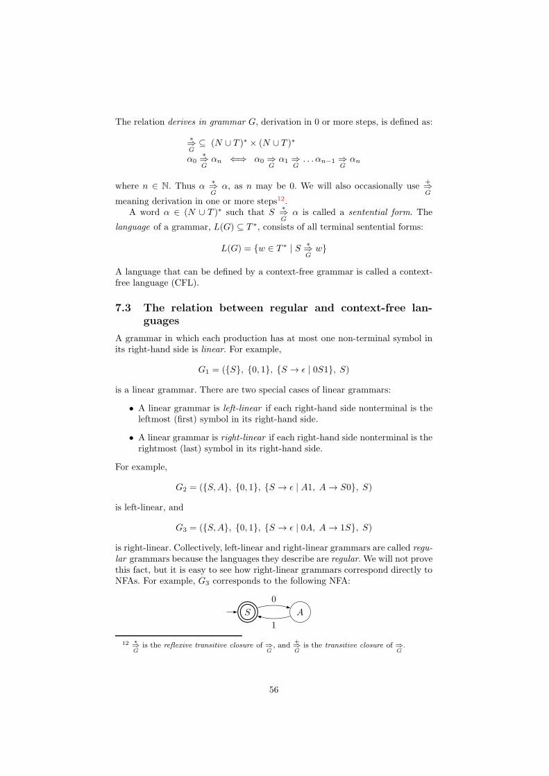
The relation derives in grammar G, derivation in 0 or more steps, is defined as:
∗⇒G
⊆ (N ∪ T )∗ × (N ∪ T )∗
α0∗⇒G
αn ⇐⇒ α0 ⇒G
α1 ⇒G
. . . αn−1 ⇒G
αn
where n ∈ N. Thus α∗⇒G
α, as n may be 0. We will also occasionally use+⇒G
meaning derivation in one or more steps12.A word α ∈ (N ∪ T )∗ such that S
∗⇒G
α is called a sentential form. The
language of a grammar, L(G) ⊆ T ∗, consists of all terminal sentential forms:
L(G) = {w ∈ T ∗ | S∗⇒G
w}
A language that can be defined by a context-free grammar is called a context-free language (CFL).
7.3 The relation between regular and context-free lan-
guages
A grammar in which each production has at most one non-terminal symbol inits right-hand side is linear. For example,
G1 = ({S}, {0, 1}, {S → ǫ | 0S1}, S)
is a linear grammar. There are two special cases of linear grammars:
• A linear grammar is left-linear if each right-hand side nonterminal is theleftmost (first) symbol in its right-hand side.
• A linear grammar is right-linear if each right-hand side nonterminal is therightmost (last) symbol in its right-hand side.
For example,
G2 = ({S,A}, {0, 1}, {S → ǫ | A1, A → S0}, S)
is left-linear, and
G3 = ({S,A}, {0, 1}, {S → ǫ | 0A, A → 1S}, S)
is right-linear. Collectively, left-linear and right-linear grammars are called regu-lar grammars because the languages they describe are regular. We will not provethis fact, but it is easy to see how right-linear grammars correspond directly toNFAs. For example, G3 corresponds to the following NFA:
S A
0
1
12 ∗⇒G
is the reflexive transitive closure of ⇒G, and
+⇒G
is the transitive closure of ⇒G.
56

Thus we see that context-free grammars can be used to describe at least someregular languages. On the other hand, some of the languages that we have shownnot to be regular are actually context-free. For example, the (linear) grammarG1 above describes the language {0n1n | n ∈ N} that we proved (theorem 6.2)not to be regular. It is worth noting that if we allow left-linear and right-linearproductions to be mixed, the resulting language is not necessarily regular. Forexample, the grammar
G′1 = ({S,A}, {0, 1}, {S → ǫ | 0A, A → S1}, S)
is equivalent to G1; i.e., describes the same, non-regular, language. Further, weproved (theorem 6.4) that the language of even-length palindromes
Lpali = {wwR | w ∈ {a, b}∗}
is not regular. The following context-free grammar is one way of defining thislanguage, demonstrating that Lpali is a context-free language:
Gpali = ({S}, {a, b}, {S → ǫ | aSa | bSb}, S)
So, what is the relation between the regular and context-free languages? Arethere languages that are regular but not context-free? The answer is no:
Theorem 7.1 All regular languages are context-free.
Again, we do not give a proof, but the idea is that regular expressions canbe translated into (regular) context-free grammars. For example, a∗b∗ can betranslated into:
({A,B}, {a, b}, {A → aA | B, B → bB | ǫ}, A)
As a consequence of theorem 7.1 and the fact that we have seen that there are atleast some languages that are context-free but not regular, we have establishedthat the regular languages form a proper subset of the context-free ones.
7.4 Derivation trees
A derivation in a context-free grammar induce a corresponding derivation treethat reflects the structure of the derivation: how each nonterminal was rewritten.As an example, consider the tree representation of the derivation of a+ (a ∗ a)in grammar Garith (section 7.2):
E
T
F
)E
T
F
a
∗T
F
a
(
+E
T
F
a
57

The central point is that the parent-child relationship reflects a derivationstep according to a production in the grammar. For example, the productionF → (E) was used once in the derivation of a+ (a ∗ a), and consequently thereis a node labelled F in the derivation tree with child nodes labelled (, E, ),ordered from left to right.
In more detail, a tree is a derivation tree for a CFG G = (N, T, P, S) iff:
1. Every node has a label from N ∪ T ∪ {ǫ}.
2. The label of the root node is S.
3. Labels of internal nodes belong to N .
4. If a node n has label A and nodes n1, n2, . . . , nk are children of n, from leftto right, with labels X1, X2, . . .Xk, respectively, then A → X1X2 . . . Xk
is a production in P .
5. If a node n has label ǫ, then n is a leaf and the only child of its parent.
Through the notion of the yield of a derivation tree, the relationship betweena derivation tree and corresponding derivations can be made precise:
• The string of leaf labels read from left to right, eliding any ǫ bar one if itis the only remaining symbol, constitute the yield of the tree.
• For a CFG G = (N, T, P, S), a string α ∈ (N ∪ T )∗ is the yield of some
derivation tree iff S∗⇒G
α.
Note that the leaf nodes may be labelled with either terminal or nonterminalsymbols. The yield is thus a sentential form (see section 7.2) in general, and notnecessarily a word in the language of the context-free grammar.
To illustrate the above point, along with elision of superfluous ǫs from theyield, consider the grammar
S → AB
A → aS | ǫ
B → Sb | ǫ
One derivation in this grammar is
S ⇒ AB ⇒ aSB ⇒ aABB
The corresponding derivation tree is
S
BA
S
BA
a
58
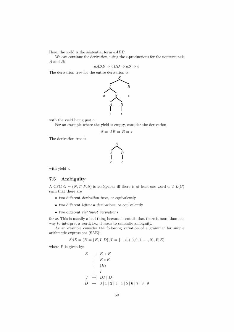
Here, the yield is the sentential form aABB.We can continue the derivation, using the ǫ-productions for the nonterminals
A and B:aABB ⇒ aBB ⇒ aB ⇒ a
The derivation tree for the entire derivation is
S
B
ǫ
A
S
B
ǫ
A
ǫ
a
with the yield being just a.For an example where the yield is empty, consider the derivation
S ⇒ AB ⇒ B ⇒ ǫ
The derivation tree is
S
B
ǫ
A
ǫ
with yield ǫ.
7.5 Ambiguity
A CFG G = (N, T, P, S) is ambiguous iff there is at least one word w ∈ L(G)such that there are
• two different derivation trees, or equivalently
• two different leftmost derivations, or equivalently
• two different rightmost derivations
for w. This is usually a bad thing because it entails that there is more than oneway to interpret a word; i.e., it leads to semantic ambiguity.
As an example consider the following variation of a grammar for simplearithmetic expressions (SAE):
SAE = (N = {E, I,D}, T = {+, ∗, (, ), 0, 1, . . . , 9}, P, E)
where P is given by:
E → E + E
| E ∗ E
| (E)
| I
I → DI | D
D → 0 | 1 | 2 | 3 | 4 | 5 | 6 | 7 | 8 | 9
59

The grammar SAE allows expressions involving numbers to be derived, unlikeGarith. Also note that this grammar is simpler in that there only is one nonter-minal (E) involved at the level of expressions proper, as opposed to three (E,T , F ) for Garith.
Consider the word 1 + 2 ∗ 3. The following derivation tree shows that thisword belongs to L(SAE):
E
E
E
I
D
3
∗E
I
D
2
+E
I
D
1
Note that the yield is the word above, 1 + 2 ∗ 3. But there is another tree withthe same yield:
E
E
I
D
3
∗E
E
I
D
2
+E
I
D
1
Thus, there is one word for which there are two derivation trees. This showsthat the grammar SAE is ambiguous.
As per the definition of ambiguity, another way to demonstrate ambiguity isto find two leftmost or two rightmost derivations for a word. It is easy to see thatthere is a one-to-one correspondence between a derivation tree and a leftmostand a rightmost derivation. To illustrate, here are the two leftmost derivationsfor 1 + 2 ∗ 3, corresponding to the first and to the second tree respectively:
E ⇒lm
E + E ⇒lm
I + E ⇒lm
D + E ⇒lm
1 + E ⇒lm
1 + E ∗ E
⇒lm
1 + I ∗ E ⇒lm
1 +D ∗ E ⇒lm
1 + 2 ∗ E
⇒lm
1 + 2 ∗ I ⇒lm
1 + 2 ∗D ⇒lm
1 + 2 ∗ 3
and
E ⇒lm
E ∗ E ⇒lm
E + E ∗ E ⇒lm
I + E ∗ E ⇒lm
D + E ∗ E
⇒lm
1 + E ∗ E ⇒lm
1 + I ∗ E ⇒lm
1 +D ∗ E ⇒lm
1 + 2 ∗ E
⇒lm
1 + 2 ∗ I ⇒lm
1 + 2 ∗D ⇒lm
1 + 2 ∗ 3
60

Note, one word, two different leftmost derivations. Thus the grammar is am-biguous. Exercise: Find the rightmost derivation corresponding to each tree.
There are two reasons for why ambiguity is problematic. The first we alreadyalluded to: semantic ambiguity. Suppose we wish to assign a meaning to a wordbeyond the word itself. In our case, the meaning might be the result of evaluatingthe expression, for instance. Then the first tree suggests that the expressionshould be read as 1+(2∗3), which evaluates to 7, while the second tree suggeststhe expression should be read as (1 + 2) ∗ 3, which evaluates to 913. Note howthe bracketing reflects the tree structure in each case. We have one word withtwo different interpretations and thus semantic ambiguity.
The other reason is that many methods for parsing, i.e. determining if agiven word belongs to the language defined by a CFG, do not work for ambiguousgrammars. In particular, this applies to efficient methods for parsing that usuallyare what we would like to use for that very reason. We return to parsing insection 10.
Fortunately, it is often possible to change an ambiguous grammar into anunambiguous one that is equivalent; i.e., the language is unchanged. Such gram-mar transformations are discussed 8. But for now, let us note that Garith wascarefully structured so as to be unambiguous. We can restructure SAE similarly:
E → E + T | T
T → T ∗ F | F
F → (E) | I
I → DI | D
D → 0 | 1 | 2 | 3 | 4 | 5 | 6 | 7 | 8 | 9
Now there is only one possible derivation tree for 1 + 2 ∗ 3:
E
T
F
I
D
3
∗T
F
I
D
2
+E
T
F
I
D
1
Convince yourself that this is the case. Note that this tree corresponds to thereading 1 + (2 ∗ 3) of the expression; i.e. a reading where multiplication hashigher precedence than addition. This is, of course, is the standard convention.
13 Strictly speaking, this is just a natural and often convenient convention, since it impliesthat the meaning of the whole can be understood in terms of the meaning of the parts in theobvious way implied by the structure of the tree. However, sometimes, in real compilers, itmight be necessary or convenient to parse things in a way that does not reflect the semanticsas directly. But then the parse tree is usually transformed later into a simplified, internalversion (an Abstract Syntax Tree), the structure of which reflects the intended semantics asdescribed here.
61

Now, if the interpretation (1 + 2) ∗ 3 is desired, explicit parentheses have tobe used. The (only!) derivation tree for this word is:
E
T
F
I
D
3
∗T
F
)E
T
F
I
D
2
+E
T
F
I
D
1
(
Note that the addition now is a subexpression (subtree) of the overall expression,which is what was desired.
7.6 Applications of context-free grammars
An important example for context-free languages is the syntax of programminglanguages. For example, the specification of the Java programming language14
[GJS+15] uses a context-free grammar to specify the syntax of Java. Anotherexample is the specification of the syntax of the language used in the G53CMPCompilers module [Nil16].
In practice, the exact details of how a grammar is presented often differs alittle bit from the conventions introduced here. The Java language specificationbeing a case in point. Further common variations include Backus-Naur form(BNF)15 and Extended Backus-Naur form (EBNF)16. But these differences areentirely superficial. For example, the symbol ::= is often used instead of →. Foranother example, EBNF introduces a shorthand notation for “zero or more of”,commonly denoted by enclosing a grammar symbol (or symbols) in curly bracesor using a Kleene-star like notation; e.g.:
A → . . . {B} . . .
or
A → . . . B∗ . . .
14 http://docs.oracle.com/javase/specs/15 https://en.wikipedia.org/wiki/Backus%E2%80%93Naur form16 https://en.wikipedia.org/wiki/Extended Backus%E2%80%93Naur form
62

It is easy to see that this iterative construct really just is a shorthand for basicproductions as it readily can be expressed by introducing an auxiliary nonter-minal and a couple of associated productions, either using left recursion or rightrecursion. The example above can be translated into the equivalent immediatelyleft-recursive (section 7.1) productions
A → . . . A1 . . .
A1 → ǫ | A1B
or into the equivalent immediately right-recursive productions
A → . . . A1 . . .
A1 → ǫ | BA1
where A1 is a the new, auxiliary, nonterminal.Note that not all syntactic aspects of common programming languages are
captured by the context-free grammar. For example, requirements regardingdeclaring variables before they are used and type correctness of expressionscannot be captured through context-free languages. However, at least in thearea of programming languages, it is common practice to use the notion of“syntactically correct” in the more limited sense of “conforming to the context-free grammar of the language”. Aspects such as type-correctness are consideredseparately.
Another application is the document type definition (DTD)17 for the SGML-family markup languages, like XML and HTML. A DTD defines the documentstructure including legal elements and attributes. It can be declared inline, asa header of the document to which the definition applies, or as an externalreference.
Extensions of context-free grammars are used in computer linguistics todescribe natural languages. In fact, as mentioned in section 1.1, context-freegrammars were originally invented by Noam Chomsky for describing naturallanguages. As an example, consider the following set of terminals, each an En-glish word:
T = {the, dog, cat, that, bites, barks, catches}
We can then define a grammar G = ({S,N,NP ,VI ,VT ,VP}, T, P, S) where Pis the following set of productions:
S → NP VPN → cat | dog
NP → the N | NP that V PVI → barks | bitesVT → bites | catchesVP → VI | VT NP
This grammar allows us to derive interesting sentences like:
the dog that catches the cat that bites barks
17 https://en.wikipedia.org/wiki/Document type definition
63

7.7 Exercises
Exercise 7.1
Consider the following Context-Free Grammar (CFG) G:
S → X | YX → aXb | ǫY → cY d | ǫ
S, X , Y are nonterminal symbols, S is the start symbol, and a, b, c, d areterminal symbols.
1. Derive the following words using the grammar G. Answer by giving theentire derivation sequence from the start symbol S:(a) ǫ(b) aabb(c) cccddd
2. Does the string aaaddd belong to the language L(G) generated by thegrammar G? Provide a brief justification.
3. Give a set expression (using set comprehensions and operations on setslike union) denoting the language L(G).
Exercise 7.2
Construct a context free grammar generating the language
L = {(ab)m(bc)n(cb)n(ba)m | m,n ≥ 1}{dn | n ≥ 0} ∪ {dn | n ≥ 2}
over the alphabet {a, b, c, d} (parentheses are only used for grouping). Note thatset concatenation has higher precedence than set union. Explain your construc-tion.
Exercise 7.3
Consider the Context-Free Grammar (CFG) G = (N, T, P, S) where N ={S,X, Y } are the nonterminal symbols, T = {a, b, c} are the terminal symbols,S is the start symbol, and the set of productions P is:
S → X | YX → aXb | abY → bY c | ǫ
Recall that the relation “derives directly in G” is a relation on strings ofterminals and non-terminals; i.e.
⇒G
⊆ (N ∪ T )∗ × (N ∪ T )∗
such that for all α, γ ∈ (N ∪ T )∗
αAγ ⇒G
αβγ ⇐⇒ A → β ∈ P
List all pairs (φ, θ) of the relation⇒G
for the cases where either φ ∈ {X,XY, aXbY c, cc}
or θ = a.
64

Exercise 7.4
Consider the following Context-Free Grammar (CFG) Exp:
T → T + T | FF → F ∗ F | PP → N(A) | (T ) | IN → f | g | hA → T | ǫI → DI | DD → 0 | 1 | 2 | 3 | 4 | 5 | 6 | 7 | 8 | 9
T , F , P , N , A, I, D are nonterminals; +, ∗, f , g, h, (, ), 0, 1, 2, 3, 4, 5, 6, 7, 8,9 are terminals; T is the start symbol.
1. Derive the following words in the grammar Exp where possible. If itis possible to derive the word, give the entire left-most derivation; i.e.always expand the left-most non-terminal of the sentential form18. If itis not possible to derive the word, give a brief explanation as to why not.(a) (789)(b) 7 + g(3 ∗ 5) ∗ (f())(c) 1 + 2 ∗ 3)(d) 1 + 7(9)
2. Draw a derivation tree for the word 7 + (8 ∗ h(1)) + 9 in the grammarExp.
3. Draw another derivation tree for the word 7+(8∗h(1))+9 from 2. Whatdoes the fact that there are two different derivation trees for one wordtell about the grammar Exp?
4. Modify the relevant productions of the grammar Exp so that a functionsymbol (one of f , g, h) can be applied to zero, one, or more arguments,separated by a single comma when there are more than one argument,instead of just zero or one argument. For example, it should be possibleto derive words like
f(2, g(), h(3 + 4))
Explain your construction.
18 Sentential form: word derivable from the start symbol.
65
8 Transformations of context-free grammars
In this section, we discuss how context free grammars can be restructured sys-tematically without changing the language that they describe. There are manyreasons for doing this, such as simplifying a grammar, putting it into somespecific form, or eliminating ambiguities.
8.1 Equivalence of context-free grammars
Two grammars G1 and G2 are equivalent iff
L(G1) = L(G2)
Whenever a grammar is being transformed, it is assumed that the resultinggrammar is equivalent to the original one.
For example, the following two grammars are equivalent:
G1:S → ǫ | A
A → a | aAG2:
S → A
A → ǫ | Aa
L(G1) = {a}∗ = L(G2). The equivalence of CFGs is in general undecidable(section 11).
8.2 Elimination of uselsss productions
In a context free grammar G = (N, T, P, S), a nonterminal X ∈ N is
• reachable iff S∗⇒ αXβ for some α, β ∈ {N ∪ T }∗
• productive iff X∗⇒ w for some w ∈ T ∗
Phrased differently, a nonterminal X is reachable if it occurs in some senten-tial form. Productions for nonterminals that are unreachable or unproductive,or where an unproductive nonterminal occurs on the right-hand side, are col-lectively knows as useless productions. Any useless production can be removedfrom a grammar without changing the language.
For example, consider the following grammar, where N = {S,A,B}, T ={a, b}, and S is the start symbol:
S → aAB | b
A → aA | a
B → bB
The nonterminal B is unproductive as there is no way to derive a word of onlyterminal symbols from it. This makes the productions S → aAB and B → bBuseless. Removing those productions leaves us with:
S → b
A → aA | a
66

But now A has clearly become an unreachable nonterminal, making the produc-tions A → aA and A → a useless too. If we remove those as well we obtain:
S → b
Of course, any terminal and nonterminals that no longer occur in any produc-tions can also be eliminated. Thus the set of nonterminals is now just {S} andthe set of terminals just {b}.
8.3 Substitution
As a direct consequence of how derivation in a grammar is defined, it followsthat an occurrence of a non-terminal in a right-hand side may be replaced by theright-hand sides of the productions for that non-terminal if done in all possibleways. This is a form of substitution.
For example, consider the following grammar fragment. We assume it in-cludes all productions for B, and we wish to eliminate the occurrence of B inthe right-hand side of the production for A:
A → XBY
B → C | D
B → ǫ
Note that there are three productions for B. By substitution, this grammarfragment can be transformed into:
A → XCY | XDY | XY
B → C | D
B → ǫ
Thus we get one new production for A for each alternative for B. Note thatwe cannot necessarily remove the productions for B: there may be other occur-rences of B in the grammar (as the above was only a fragment). However, ifsubstitution renders some symbols unreachable, then the productions for thosesymbols become useless and can consequently be removed (section 8.2).
Substitution can of course also be performed on recursive productions. Thatis often not very useful, though, as the productions just get bigger and more nu-merous without eliminating any nonterminals. For example, assume the follow-ing productions are all productions for A in some grammar. Note that A → Abis recursive (immediately left-recursive, as it happens):
A → ǫ | Ab
We can substitute the right-hand sides of all productions for A for the oneoccurrence of A in the right-hand side of A → Ab. That would leave us with:
A → ǫ | b | Abb
Thus we did not gain anything here, unless there was some specific reason forwanting a single production that shows that A can yield a single b.
67
8.4 Left factoring
Sometimes it is useful to factor out a common prefix of the right-hand sides ofa group of productions. This is called left factoring. Left factoring can make agrammar easier to read and understand as it captures a recurring pattern in oneplace. It is sometimes also necessary for putting a grammar into a form suitablefor use with certain parsing methods (section 10).
Consider the following two productions for A. Note the common prefix XY :
A → XYX | XY ZZY
After left factoring:
A → BX | BZZY
B → XY
8.5 Disambiguating context-free grammars
Given an ambiguous context-free grammar G, it is often possible to constructan equivalent but unambiguous grammar G′. Some context-free languages areinherently ambiguous, meaning that every CFG generating the language is neces-sarily ambiguous, but most languages of practical interest, such as programminglanguages, can be given unambiguous CFGs.
In this section, we focus on how expression languages (like arithmetic expres-sions or regular expressions) can be given unambiguous CFGs by structuringthe grammar to account for operator precedence and operator associativity.
The following is a CFG for simple arithmetic expressions. For simplicity, weonly consider the numbers 0, 1, and 2:
E → E + E | E ∗ E | E ↑ E | (E) | N
N → 0 | 1 | 2
E and N are nonterminals, E is the start symbol, +, ∗, ↑, (, ), 0, 1, 2 areterminals. The grammar is ambiguous. For example, the word 0+1+2 has twodifferent leftmost derivations:
E ⇒lm
E + E ⇒lm
N + E ⇒lm
0 + E ⇒lm
0 + E + E ⇒lm
0 +N + E ⇒lm
0 + 1 + E
⇒lm
0 + 1 +N ⇒lm
0 + 1 + 2
E ⇒lm
E + E ⇒lm
E + E + E ⇒lm
N + E + E ⇒lm
0 + E + E ⇒lm
0 +N + E
⇒lm
0 + 1 + E ⇒lm
0 + 1 +N ⇒lm
0 + 1 + 2
We now wish to construct an equivalent but unambiguous version of thethe above grammar by making it reflect the following conventions regardingoperator precedence and associativity:
Operators Precedence Associativity
↑ highest right∗ medium left+ lowest left
68

For example, the word1 + 2 ∗ 2 ↑ 2 ↑ 2 + 0
should be read as(1 + (2 ∗ (2 ↑ (2 ↑ 2)))) + 0
That is, the structure of the (one and only) derivation tree should reflect thisreading.
To impart operator precedence on the grammar, it has to be stratified : Firstthe expressions have to be partitioned into different categories of expressions,one category for each operator precedence level. We thus need to introduceone nonterminal (or syntactic category) for each precedence level. Then it mustbe arranged so that expressions belonging to the category for operators of oneprecedence level only occur as subexpressions of expressions belonging to thecategory for operators of the next lower precedence level. Bracketing (enclosingan expression in some form of parentheses) should have higher precedence thanany operator. Bracketed subexpressions should thus only be allowed as subex-pressions of expressions in the category for the highest operator precedence. Theexpression enclosed in the parentheses, however, should be of the category forthe lowest operator precedence.
In our example, there are three operator precedence levels, so we introducethree additional nonterminals (E1, E2, E3) to stratify the grammar into fourlevels: one level for each operator precedence category, and one more for theinnermost expression level, the subexpressions of expressions involving operatorsof the highest precedence. The resulting grammar is:
E → E1 + E1 | E1
E1 → E2 ∗ E2 | E2
E2 → E3 ↑ E3 | E3
E3 → (E) | N
N → 0 | 1 | 2
This grammar is fine in that it is unambiguous. But for practical purposes,it is inconvenient as expressions involving more than one operator at the samelevel has to be explicitly bracketed. For example, the word 0 + 1 + 2 cannot bederived in this grammar (try it!), but a user of this little expression languagewould have to write either (0 + 1) + 2 or 0 + (1 + 2).
This is where operator associativity comes into the picture: by adopting aconvention regarding associativity, expressions involving more than operator ofsome specific precedence level can be implicitly bracketed. In our example, + isleft-associative (as per standard mathematical conventions), which means theword 0+1+2 should be read as (0+1)+2; i.e. the derivation tree for 0+1+2should branch to the left, suggesting that 0+1 is a subexpression of the overallexpression.
Imparting of associativity is achieved by making productions for left -associ-ative operators left -recursive, and those for right -associative operators right -recursive, as this results in the desired left-branching or right-branching struc-ture, respectively, of the derivation tree. Note that the requirement that subex-pressions at one precedence level must all be expressions at next higher prece-dence level is relaxed a little, but only in a way that does not make the grammarunambiguous.
69

In our example, the operators + and ∗ are left-associative, and the operator↑ is right-associative. We thus make the corresponding productions left- andright-recursive, respectively, arriving at the final version of the grammar:
E → E + E1 | E1
E1 → E1 ∗ E2 | E2
E2 → E3 ↑ E2 | E3
E3 → (E) | N
N → 0 | 1 | 2
This grammar is (again) unambiguous, but now allows words like 0 + 1 + 2.Verify that there only is one derivation tree, and that this has the desired left-branching structure!
As an example, let us consider the word 1 + 2 ∗ 2 ↑ 2 ↑ 2 + 0 from above.Recall that we want the reading (1+ (2 ∗ (2 ↑ (2 ↑ 2)))) + 0. The derivation treefor the word in the final version of the grammar is:
E
E1
E2
E3
N
0
+E
E1
E2
E2
E2
E3
N
2
↑E3
N
2
↑E3
N
2
∗E1
E2
E3
N
2
+E
E1
E2
E3
N
1
Make sure you understand how the branching structure corresponds to the de-sired reading of the word; i.e., how precedence and associativity allowed forimplicit bracketing. As an exercise, draw the derivation tree for the explicitlybracketed word, and compare the structure of the two trees. The trees will notbe the same, of course, as the words are not the same (as words, symbol bysymbol), but the branching structure (what is a subexpression of what) willagree.
8.6 Elimination of left recursion
A CFG is left-recursive if there is some non-terminal A such that A+⇒ Aα19.
Certain parsing methods cannot handle left-recursive grammars. An exampleis recursive decent parsing as described in section 10. If we want to use sucha parsing method for parsing a language L = L(G) given by a left-recursive
19 Recall that+⇒ means derives in one or more steps; i.e., the transitive closure of ⇒.
70

grammar G, then it first has to be transformed into an equivalent grammar G′
that is not left-recursive.We first consider immediate left recursion (section 7.1); i.e., productions of
the form A → Aα. We assume that α cannot derive ǫ.The key idea of the transformation is simple. Let us first consider a simplified
scenario, with one immediately left-recursive production for a nonterminalA andone non-recursive production:
A → Aα
A → β
Then observe that all strings derivable from A using these two productions havethe form β(α)∗ once the last A has been replaced by β; i.e., β followed by zero ormore α. Now it is easy to see that the following alternative grammar generatesstrings of exactly the same form:
A → βA′
A′ → αA′ | ǫ
This is arguably a more direct way to generate strings of the form β(α)∗. Inessence, the productions say: “start with β, and then tag on zero or more α”.
We now generalise and formalise this idea. In order to transform an immedi-ately left-recursive grammar to an equivalent grammar that is not left recursive,proceed as follows. For each nonterminal A defined by some left-recursive pro-duction, group the productions for A
A → Aα1 | Aα2 | . . . | Aαm | β1 | β2 | . . . | βn
such that no βi begins with an A. Then replace the A productions by
A → β1A′ | β2A
′ | . . . | βnA′
A′ → α1A′ | α2A
′ | . . . | αmA′ | ǫ
Assumption: no αi derives ǫ.To illustrate, consider the immediately left-recursive grammar
S → A | B
A → ABc | AAdd | a | aa
B → Bee | b
Applying the transformation rules above yields the following equivalent right-recursive grammar:
S → A | B
A → aA′ | aaA′
A′ → BcA′ | AddA′ | ǫ
B → bB′
B′ → eeB′ | ǫ
Let us do a sanity check on the new grammar by picking a word in thelanguage of the original grammar and make sure it can also be derived in thenew grammar. The derivation of the word should ideally make use of all recursiveproductions in the grammar. Let us pick the word aabeeeecddbeec. The followingis the derivation tree for this word in the original grammar, demonstrating thatthe word indeed is in the language generated by the grammar:
71

S
A
cB
eeB
b
A
ddA
cB
eeB
eeB
b
A
a
A
a
The derivation tree for the same word in the transformed grammar:
S
A
A′
A′
A′
ǫ
cB
B′
B′
ǫ
ee
b
ddA
A′
A′
ǫ
cB
B′
B′
B′
ǫ
ee
ee
b
a
a
Note that, while the yield is the same in both cases, the structure of the treesare very different: the first tree is more left-branching, due to the left recursion,and the other more right-branching, due to the right-recursion.
To eliminate general left recursion, the grammar is first transformed into animmediately left-recursive grammar through systematic substitution (section8.3). After this the elimination scheme set out above can be applied.
Consider the following grammar. Note that no production is immediatelyleft-recursive:
A → BaB
B → Cb | ǫ
C → Ab | Ac
The grammar is, however, left recursive because, for example, A ⇒ BaB ⇒
CbaB ⇒ AbbaB. Thus we have A+⇒ Aα (for α = bbaB in this case), demon-
strating that the grammar is left recursive.
72

To eliminate the left recursion, let us first transform this grammar into anequivalent immediately left-recursive grammar. Let us start by eliminating Cby substituting all alternatives for C into the right-hand side of the productionB → Cb. Note that this makes C an unreachable nonterminal, making theproductions for C useless meaning they can be removed (section 8.2):
A → BaB
B → Abb |Acb | ǫ
Then we can eliminate B wherever it occurs in the leftmost position of a right-hand side in the productions for A. The grammar is now immediately left-recursive:
A → AbbaB | AcbaB | aB
B → Abb |Acb | ǫ
Alternatively, B can be eliminated completely from the productions for A, mak-ing B an unreachable terminal allowing the productions for B to be removed:
A → AbbaAbb | AcbaAbb | aAbb
| AbbaAcb | AcbaAcb | aAcb
| Abba | Acba | a
Let us go with the smaller version (fewer productions):
A → AbbaB | AcbaB | aB
B → Abb |Acb | ǫ
Only the productions for A are immediately left-recursive. Applying the trans-formation to eliminate left recursion gives us:
A → aBA′
A′ → bbaBA′ | cbaBA′ | ǫ
B → Abb |Acb | ǫ
Note that A appears to the left in B-productions; yet the grammar is no longerleft-recursive. Why?
73

8.7 Exercises
Exercise 8.1
The grammar Exp from exercise 7.4 is ambiguous. Fix this problem; i.e., modifythe grammar, without changing the language of the grammar, so that all wordsin the language have exactly one derivation tree. You do not need to prove thatthis holds for the resulting grammar, but you should explain what you did andwhy.
Exercise 8.2
The following context-free grammar is immediately left-recursive:
S → Sa | XbS | a
X → XXX | Y Y Y | XY Y | Y Y X
Y → cY | dY | e
S, X , and Y are nonterminals, S is the start symbol, and a, b, c, d, and e areterminals.
Transform it into an equivalent right-recursive grammar. Explicitly showthe result of the grouping step in addition to the final result after applying theactual transformation step to the productions that need transformation.
74

9 Pushdown Automata
We will now consider a new notion of automata Pushdown Automata (PDA).PDAs are finite automata with a stack; i.e., a data structure that can be usedto store an arbitrary number of symbols (hence PDAs have an infinite set ofstates) but which can be only accessed in a last-in-first-out (LIFO) fashion.The languages that can be recognized by PDA are precisely the context-freelanguages.
9.1 What is a pushdown automaton?
A Pushdown Automaton P = (Q,Σ,Γ, δ, q0, Z0, F ) is given by the followingdata
• A finite set Q of states,
• A finite set Σ of input symbols (the alphabet),
• A finite set Γ of stack symbols,
• A transition function
δ ∈ Q× (Σ ∪ {ǫ})× Γ → Pfin(Q × Γ∗)
Here Pfin(A) are the finite subsets of a set; i.e., this can be defined as
Pfin(A) = {X | X ⊆ A ∧X is finite.}
Thus, PDAs are in general nondeterministic, since they may have a choiceof transitions from any state. However, there are always only finitely manychoices.
• An initial state q0 ∈ Q,
• An initial stack symbol Z0 ∈ Γ,
• A set of final states F ⊆ Q.
As an example we consider a PDA P that recognizes the language of evenlength palindromes over Σ = {0, 1}: L = {wwR | w ∈ {0, 1}∗}. Intuitively, thisPDA pushes the input symbols on the stack until it guesses that it is in themiddle and then it compares the input with what is on the stack, popping ofsymbols from the stack as it goes. If it reaches the end of the input precisely atthe time when the stack is empty, it accepts.
P0 = ({q0, q1, q2}, {0, 1}, {0, 1,#}, δ, q0,#, {q2})
75

where δ is given by the following equations:
δ(q0, 0,#) = {(q0, 0#)}δ(q0, 1,#) = {(q0, 1#)}δ(q0, 0, 0) = {(q0, 00)}δ(q0, 1, 0) = {(q0, 10)}δ(q0, 0, 1) = {(q0, 01)}δ(q0, 1, 1) = {(q0, 11)}δ(q0, ǫ,#) = {(q1,#)}δ(q0, ǫ, 0) = {(q1, 0)}δ(q0, ǫ, 1) = {(q1, 1)}δ(q1, 0, 0) = {(q1, ǫ)}δ(q1, 1, 1) = {(q1, ǫ)}δ(q1, ǫ,#) = {(q2, ǫ)}δ(q, w, z) = ∅ everywhere else
To save space we may abbreviate this by writing:
δ(q0, x, z) = {(q0, xz)}δ(q0, ǫ, z) = {(q1, z)}δ(q1, x, x) = {(q1, ǫ)}δ(q1, ǫ,#) = {(q2, ǫ)}δ(q, x, z) = ∅ everywhere else
where q ∈ Q, x ∈ Σ, z ∈ Γ. We obtain the previous table by expanding all thepossibilities for q, x, z.
We draw the transition diagram of P by labelling each transition with atriple x, Z, γ with x ∈ Σ, Z ∈ Γ, γ ∈ Γ∗:
q0 q1 q2
x, z, xz
ǫ, z, z
x, x, ǫ
ǫ,#, ǫ
9.2 How does a PDA work?
At any time the state of the computation of a PDA P = (Q,Σ,Γ, δ, q0, Z0, F ) isgiven by:
• the state q ∈ Q the PDA is in,
• the input string w ∈ Σ∗ that still has to be processed,
• the contents of the stack γ ∈ Γ∗.
Such a triple (q, w, γ) ∈ Q×Σ∗×Γ∗ is called an Instantaneous Description (ID).We define a relation ⊢
P⊆ ID×ID between IDs that describes how the PDA can
change from one ID to the next one. Since PDAs in general are nondeterministicthis is a relation (not a function); i.e., there may be more than one possibility.
There are two possibilities for ⊢P:
1. (q, xw, zγ) ⊢P(q′, w, αγ) if (q′, α) ∈ δ(q, x, z)
76

2. (q, w, zγ) ⊢P(q′, w, αγ) if (q′, α) ∈ δ(q, ǫ, z)
In the first case the PDA reads an input symbol and consults the transitionfunction δ to calculate a possible new state q′ and a sequence of stack symbolsα that replaces the currend symbol on the top z.
In the second case the PDA ignores the input and silently moves into a newstate and modifies the stack as above. The input is unchanged.
Consider the word 0110. What are possible sequences of IDs for P0 startingwith (q0, 0110,#) ?
(q0, 0110,#) ⊢P0
(q0, 110, 0#) 1. with (q0, 0#) ∈ δ(q0, 0,#)
⊢P0
(q0, 10, 10#) 1. with (q0, 10) ∈ δ(q0, 1, 0)
⊢P0
(q1, 10, 10#) 2. with (q1, 1) ∈ δ(q0, ǫ, 1)
⊢P0
(q1, 0, 0#) 1. with (q1, ǫ) ∈ δ(q1, 1, 1)
⊢P0
(q1, ǫ,#) 1. with (q1, ǫ) ∈ δ(q1, 0, 0)
⊢P0
(q2, ǫ, ǫ) 2. with (q2, ǫ) ∈ δ(q1, ǫ,#)
We write (q, w, γ)∗
⊢P(q′, w′, γ) if the PDA can move from (q, w, γ) to (q′, w′, γ′)
in a (possibly empty) sequence of moves. Above we have shown that
(q0, 0110,#)∗
⊢P0
(q2, ǫ, ǫ).
However, this is not the only possible sequence of IDs for this input. E.g.the PDA may just guess the middle wrong:
(q0, 0110,#) ⊢P0
(q0, 110, 0#) 1. with (q0, 0#) ∈ δ(q0, 0,#)
⊢P0
(q1, 110, 0#) 2. with (q1, 0) ∈ δ(q0, ǫ, 0)
We have shown (q0, 0110,#)∗
⊢P0
(q1, 110, 0#). Here the PDA gets stuck as there
is no state after (q1, 110, 0#).If we start with a word that is not in the language L (like 0011) then the
automaton will always get stuck before reaching a final state.
9.3 The language of a PDA
There are two ways to define the language of a PDA P = (Q,Σ,Γ, δ, q0, Z0, F )(L(P ) ⊆ Σ∗) because there are two notions of acceptance:
Acceptance by final state
L(P ) = {w | (q0, w, Z0)∗
⊢P(q, ǫ, γ) ∧ q ∈ F}
That is the PDA accepts the word w if there is any sequence of IDs startingfrom (q0, w, Z0) and leading to (q, ǫ, γ), where q ∈ F is one of the finalstates. Here it doesn’t play a role what the contents of the stack are atthe end.
77

In our example the PDA P0 would accept 0110 because (q0, 0110,#)∗
⊢P0
(q2, ǫ, ǫ) and q2 ∈ F . Hence we conclude 0110 ∈ L(P0).
On the other hand since there is no successful sequence of IDs startingwith (q0, 0011,#) we know that 0011 /∈ L(P0).
Acceptance by empty stack
L(P ) = {w | (q0, w, Z0)∗
⊢P(q, ǫ, ǫ)}
That is the PDA accepts the word w if there is any sequence of IDs startingfrom (q0, w, Z0) and leading to (q, ǫ, ǫ), in this case the final state plays norole.
If we specify a PDA for acceptance by empty stack we will leave out theset of final states F and just use P = (Q,Σ,Γ, δ, q0, Z0).
Our example automaton P0 also works if we leave out F and use accep-tance by empty stack.
We can always turn a PDA that uses one acceptance method into one thatuses the other. Hence, both acceptance criteria specify the same class of lan-guages.
9.4 Deterministic PDAs
We have introduced PDAs as nondeterministic machines that may have severalalternatives how to continue. We now define Deterministic Pushdown Automata(DPDA) as those that never have a choice.
To be precise we say that a PDA P = (Q,Σ,Γ, δ, q0, Z0, F ) is deterministic(is a DPDA) iff
|δ(q, x, z)|+ |δ(q, ǫ, z)| ≤ 1
Remember, that |X | stands for the number of elements in a finite set X .That is: a DPDA may get stuck but it has never any choice.In our example the automaton P0 is not deterministic, e.g. we have δ(q0, 0,#) =
{(q0, 0#)} and δ(q0, ǫ,#) = {(q1,#)} and hence |δ(q0, 0,#)|+ |δ(q0, ǫ,#)| = 2.Unlike the situation for finite automata, there is in general no way to trans-
late a nondeterministic PDA into a deterministic one. Indeed, there is no DPDAthat recognizes the language L! Nondeterministic PDAs are more power-ful than deterministic PDAs.
However, we can define a similar language L′ over Σ = {0, 1, $} that can berecognized by a deterministic PDA:
L′ = {w$wR | w ∈ {0, 1}∗}
That is L′ contains palindroms with a marker $ in the middle, e.g. 01$10 ∈ L′.We define a DPDA P ′ for L′:
P ′ = ({q0, q1, q2}, {0, 1, $}, {0, 1,#}, δ′, q0,#, {q2})
78

where δ′ is given by:
δ′(q0, x, z) = {(q0, xz)} x ∈ {0, 1}, z ∈ {0, 1,#}δ′(q0, $, z) = {(q1, z)} z ∈ {0, 1,#}δ′(q1, x, x) = {(q1, ǫ)} x ∈ {0, 1}δ′(q1, ǫ,#) = {(q2, ǫ)}δ′(q, x, z) = ∅ everywhere else
The transition graph is:
q0 q1 q2
x, z, xz
$, z, z
x, x, ǫ
ǫ,#, ǫ
We can check that this automaton is deterministic. In particular the 3rd and4th line cannot overlap because # is not an input symbol.
In contrast to PDAs in general, the two acceptance methods are not equiv-alent for DPDAs: acceptance by final state makes it possible to define a biggerclass of langauges. We will consequently always use acceptance by final state forDPDAs in the following.
9.5 Context-free grammars and push-down automata
Theorem 9.1 For a language L ⊆ Σ∗ the following two statements are equiv-alent:
1. L is given by a CFG G, L = L(G).
2. L is the language of a PDA P , L = L(P ).
To summarize: Context-Free Languages (CFLs) can be described by a Context-Free Grammar (CFG) and can be processed by a pushdown automaton.
We will he only show how to construct a PDA from a grammar - the otherdirection is shown in [HMU01] (6.3.2, pp. 241).
Given a CFG G = (V,Σ, P, S), we define a PDA
P (G) = ({q0}, Σ, V ∪Σ, δ, q0, S)
where δ is defined as follows:
δ(q0, ǫ, A) = {(q0, α) | A → α ∈ P} for all A ∈ Vδ(q0, a, a) = {(q0, ǫ)} for all a ∈ Σ.
We haven’t given a set of final states because we use acceptance by empty stack.Yes, we use only one state!
Take as an example
G = ({E, T, F}, {(, ), a, +, *}, E, P )
where the set of productions P are given by
E → T | E +T
T → F | T *F
F → a | (E )
79

we define
P (G) = ({q0}, {(, ), a, +, *}, {E, T, F, (, ), a, +, *}, δ, q0, E)
where
δ(q0, ǫ, E) = {(q0, T ), (q0, E+T )}
δ(q0, ǫ, T ) = {(q0, F ), (q0, T*F )}
δ(q0, ǫ, F ) = {(q0, a), (q0, (E))}
δ(q0, (, () = {(q0, ǫ)}
δ(q0, ), )) = {(q0, ǫ)}
δ(q0, a, a) = {(q0, ǫ)}
δ(q0, +, +) = {(q0, ǫ)}
δ(q0, *, *) = {(q0, ǫ)}
δ(q, x, z) = ∅ everywhere else
How does the P (G) accept a+(a*a)?
(q0, a+(a*a), E) ⊢ (q0, a+(a*a), E+T )
⊢ (q0, a+(a*a), T+T )
⊢ (q0, a+(a*a), F+T )
⊢ (q0, a+(a*a), a+T )
⊢ (q0, +(a*a), +T )
⊢ (q0, (a*a), T )
⊢ (q0, (a*a), F )
⊢ (q0, (a*a), (E))
⊢ (q0, a*a), E))
⊢ (q0, a*a), T))
⊢ (q0, a*a), T*F ))
⊢ (q0, a*a), F*F ))
⊢ (q0, a*a), a*F ))
⊢ (q0, *a), *F))
⊢ (q0, a), F))
⊢ (q0, a), a))
⊢ (q0, ), ))
⊢ (q0, ǫ, ǫ)
Hence a+(a*a) ∈ L(P (G)).This above example illustrates the general idea:
w ∈ L(G) ⇐⇒ S∗⇒ w
⇐⇒ (q0, w, S)∗
⊢ (q0, ǫ, ǫ)
⇐⇒ w ∈ L(P (G))
The automaton we have constructed is very nondeterministic: Whenever wehave a choice between different rules the automaton may silently choose one ofthe alternatives.
80

10 Recursive-Descent Parsing
10.1 What is parsing?
According to Merriam-Webster OnLine20 parse means:
To resolve (as a sentence) into component parts of speech and de-scribe them grammatically.
In a computer science context, we take this to mean answering whether or not
w ∈ L(G)
for a CFG G by analysing the structure of w according to G; i.e. to recognisethe language generated by a grammar G.
A parser is a program that carries out parsing. For a CFG, this amounts toa realisation of a PDA. For most practical applications, a parser will also returna structured representation of a word w ∈ L(G). This could be the derivation(or parse) tree for the word, or, more commonly, a simplified version of this, a socalled Abstract Syntax Tree. Further, for a word not in the language, w /∈ L(G),a practical parser would normally provide an error message explaining why. Animportant application of parsers is in the front-end of compilers and interpreterswhere they turn a text-based representation of a program into a structuredrepresentation for further analysis and translation or execution.
In this section we study how to systematically construct a parser from agiven CFG using the recursive-decent parsing method. To make the discussionconcrete, we implement the parsers we develop in Haskell. Thus you can easilytry out the examples in this section yourself using a Haskell system such asGHCi, and it is recommended that you do so! That said, we are essentially justusing a small fragment of Haskell as a notation for writing simple functions,so it should not be difficult to follow the development even if you are not veryfamiliar with Haskell. There are plenty of Haskell resources on-line, both forlearning and for downloading and installing Haskell systems21.
10.2 Parsing strategies
There are two basic strategies for parsing: top-down and bottom up.
• A top-down parser attempts to carry out a derivation matching the inputstarting from the start symbol; i.e., it constructs the parse tree for theinput from the root downwards in preorder.
• A bottom-up parser tries to construct the parse tree from the leaves up-wards by using the productions “backwards”.
Top-down parsing is, in essence, what we have been doing so far wheneverwe have derived some specific word in a language from the start symbol of agrammar generating that language. For example, consider the grammar:
S → aSa | bSb | a | b
20 http://www.webster.com21 http://www.haskell.org, http://learnyouahaskell.com
81

If given a string ababa, a top-down parser for this grammar would try to derivethis string from the start symbol S and thus proceed as:
S ⇒ aSa ⇒ abSba ⇒ ababa
If we draw the derivation tree after each derivation step, we see how the treegets constructed from the root downwards:
S S
aSa
S
aS
bSb
a
S
aS
bS
a
b
a
In contrast, a bottom-up parser would start from the leaves, and step bystep group them together by applying productions in reverse:
ababa ⇐ abSba ⇐ aSa ⇐ S
This is a rightmost derivation in reverse. The derivation tree thus gets con-structed from the bottom upwards:
a
S
a
S
bS
a
b
S
aS
bS
a
b
a
The key difficulty of bottom-up parsing is to decide when to reduce. For example,in this case, how does the parser know not to reduce neither the first inputsymbol a nor the second input symbol b to S, but wait until it sees the middlea and only then do the first reduction step? Such questions are answered by LRparsing theory22 We will not consider LR parsing further here, except notingthat it is covered in more depth in the Compilers module [Nil16] that builds onmuch of the material in this module. Instead we turn our attention to recursive-decent parsing, which is a type of top-down parsing.
10.3 Basics of recursive-descent parsing
Recursive-descent parsing is a way to implement top-down parsing. We are justgoing to focus on the language recognition problem: w ∈ L(G)? This suggeststhe following type for the parser:
parser :: [Token] -> Bool
Token is “compiler speak” for (input) symbol; i.e., an element of the alphabet.Consider a typical production in some CFG G:
S → AB
22 https://en.wikipedia.org/wiki/LR parser
82

Let L(X) be the language {w ∈ T ∗ | X∗⇒G
w}, X ∈ N . Note that
w ∈ L(S) ⇐ ∃w1, w2 . w = w1w2
∧ w1 ∈ L(A)∧ w2 ∈ L(B)
That is, given a parser for L(A) and a parser for L(B), we can construct a parserfor L(S) by asking the first parser if a prefix w1 of w belongs to L(A), and thenasking the other parser if the remaining suffix w2 of w belongs to L(B). If theanswer two both questions is yes, then w belongs to L(S).
However, we need to find the right way to divide the input word w! Ingeneral, there are |w|+1 possibilities. We could, of course, blindly try them all.But as the prefix and suffix recursively also have to be split in all possible ways,and so on until we get down to individual akphabet symbols, it is clear thatthis approach would lead to a combinatorial explosion that would render sucha parser useless for all but very short words.
Instead we need to let the input guide the search. To that end, we initiallyadopt the following idea:
• Each parser tries to derive a prefix of the input according to the produc-tions for the nonterminal
• Each parser returns the remaining suffix if successful, allowing this to bepassed to the next parser for analysis.
This gives us the following refined type for parsers:
parseX :: [Token] -> Maybe [Token]
Recall that Maybe is Haskell’s option type:
data Maybe a = Nothing | Just a
Of course, we should be a little suspicious: There could be more than oneprefix derivable from a non-terminal, and if so, how can we then know whichone to pick? Picking the wrong prefix might make it impossible to derive thesuffix from the non-terminal that follows. We will return to these points later.
Now we can construct a parser for L(S)
S → AB
in terms of parsers for L(A) and L(B):
parseS :: [Token] -> Maybe [Token]
parseS ts =
case parseA ts of
Nothing -> Nothing
Just ts’ ->
case parseB ts’ of
Nothing -> Nothing
Just ts’’ -> Just ts’’
Note that the case analysis on the result of parseB ts’ simply passes on theresult unchanged. Thus we can simplify the code to:
83

parseS :: [Token] -> Maybe [Token]
parseS ts =
case parseA ts of
Nothing -> Nothing
Just ts’ -> parseB ts’
This approach is called recursive-descent parsing because the parse func-tions (usually) end up being (mutually) recursive. What does this have to dowith realising a PDA? Fundamental to the implementation of a recursive com-putation is a that keeps track of the state of the computation and allows forsubcomputations (to any depth). In a language that supports recursive functionsand procedures, the stack is usually not explicitly visible, but internally, it is acentral datastructure. Thus, a recursive-descent parser is a kind of PDA.
Let us develop this example a little further into code that can be executed.First, for simplicity, let us pick the type Char for token:
type Token = Char
Recall that (basic) strings are just lists of characters in Haskell; that is, String =[Char] = [Token]. Thus, a string literal like "abcd" is just a shorthand notationfor the list of characters [’a’,’b’,’c’,’d’].
Now, suppose the productions for A and B are the following
A → a
B → b
Thus, in this case, it is clear that if the parsing function parseA for the non-terminal A sees input starting with an a, then that a is the desired prefix, andwhatever remains of the input is the suffix that should be returned as part ifthe indication of having been able to successfully derive a prefix of the inputfrom the nonterminal in question. Otherwise, if the input does not start withan a, it is equally clear that it is not possible to derive any prefix of the inputfrom the nonterminal A, and the parsing function must thus indicate failure. Inessence, this is how the input is used to guide the search for the right prefix.
We can implement parseA in Haskell, using pattern matching, as follows:
parseA :: [Token] -> Maybe [Token]
parseA (’a’ : ts) = Just ts
parseA _ = Nothing
The case and code for the parsing function parseB for the nonterminal B is ofcourse analogous:
parseB :: [Token] -> Maybe [Token]
parseB (’b’ : ts) = Just ts
parseB _ = Nothing
Now we can evaluate parseA, parseB, and parseS on "abcd" with the fol-lowing results:
parseA "abcd" ⇒ Just "bcd"
parseB "abcd" ⇒ Nothing
parseS "abcd" ⇒ Just "cd"
84

This tells us that a prefix of abcd can be derived from A, leaving a remainingsuffix bcd, that no prefix of abcd can be derived from B, but that a prefix ofabcd also can be derived from S, leaving a suffix cd, as we would expect.
10.4 Handling choice
Of course, there are usually more than one one production for a nonterminal.Thus need a way to handle choice, as in
S → AB | CD
We are first going to consider the case when the choice is obvious, as in
S → aAB | cCD
That is, we assume it is manifest from the grammar that we can choose betweenproductions with a one-symbol lookahead.
As an example, let us construct a parser for the grammar:
S → aA | bBA
A → aA | ǫ
B → bB | ǫ
We are going to need one parsing function for each non-terminal:
• parseS :: [Token] -> Maybe [Token]
• parseA :: [Token] -> Maybe [Token]
• parseB :: [Token] -> Maybe [Token]
We again take type Token = Char for simplicity.Code for parseS. Note how the pattern matching makes use of a one-symbol
lookahead to chose between the two productions for S:
parseS :: [Token] -> Maybe [Token]
parseS (’a’ : ts) =
parseA ts
parseS (’b’ : ts) =
case parseB ts of
Nothing -> Nothing
Just ts’ -> parseA ts’
parseS = Nothing
The code for parseA and parseB similarly make use of the one-symbol looka-head to chose between productions, but this time, because A ⇒ ǫ and B ⇒ ǫ, itis not a syntax error if the next token is not, respectively, a and b. Thus bothfunctions can succeed without consuming any input:
parseA :: [Token] -> Maybe [Token]
parseA (’a’ : ts) = parseA ts
parseA ts = Just ts
parseB :: [Token] -> Maybe [Token]
parseB (’b’ : ts) = parseB ts
parseB ts = Just ts
85

Now consider a more challenging scenario:
S → aA | aBA
A → aA | ǫ
B → bB | ǫ
In the parsing function parseS for nonterminal S, should parseA or parseB becalled once a has been read?
We could try the alternatives in order; i.e., a limited form of backtracking:
parseS (’a’ : ts) =
case parseA ts of
Just ts’ -> Just ts’
Nothing ->
case parseB ts of
Nothing -> Nothing
Just ts’ -> parseA ts’
Of course, the choice to try parseA first is arbitrary, a point we will revisitshortly.
Similarly, there are two alternatives for the nonterminalA. In fact, we alreadyencountered this situation above, and as we did there, let us try to consume aninput prefix (here a) if possible, and only if that is not possible succeed withoutconsuming any input:
parseA :: [Token] -> Maybe [Token]
parseA (’a’ : ts) = parseA ts
parseA ts = Just ts
The code for B is of course similar. This may seem like an obvious ordering:after all, if we opted to “try” without consuming any input first, then that wouldalways succeed, and no other alternatives would ever be tried. Nevertheless,picking the order we did still amounts to an arbitrary choice, and in fact it isnot always the right one.
The problem here is that limited backtracking is not an exhaustive search.For many grammars, there simply is no one order that always will work, meaningthat a parser that nevertheless commits to one particular order is liable to getstuck in “blind alleys”.
Consider the following grammar
S → AB
A → aA | ǫ
B → ab
and corresponding parsing functions:
parseA (’a’ : ts) = parseA ts
parseA ts = Just ts
parseB (’a’ : ’b’ : ts) = Just ts
parseB ts = Nothing
86

parseS ts =
case parseA ts of
Nothing -> Nothing
Just ts’ -> parseB ts’
Will it work? Let us try it on ab. Clearly derivable from the grammar:
S ⇒ AB ⇒ B ⇒ ab
However, if we run our parser on "ab":
parseS "ab" ⇒ Nothing
Our parser thus says “no”. Why? Because
parseA "ab" ⇒ Just "b"
That is, the code for parseA committed to the choice A → a too early and willnever try A → ǫ. That was the wrong choice in this case and the parser gotstuck in a “blind alley”.
Would it have been better to try A → ǫ first? Then the parser would workfor the word ab, but it would still fail on other words that should be accepted,such as aab. To successfully parse that word, parseA must somehow consumethe first a but not the second, and neither ordering of the productions for A willachieve that.
One principled approach addressing this dilemma is to try all alternatives;i.e., full backtracking (aka list of successes):
• Each parsing function returns a list of all possible suffixes. Type:
parseX :: [Token] -> [[Token]]
• Translate A → α | β into
parseA ts = parseAlpha ts ++ parseBeta ts
• An empty list indicates no possible parsing.
However:
• Full backtracking is computationally expensive.
• In error reporting, it becomes difficult to pinpoint the exact location of asyntax error: where exactly lies the problem if it only after an exhaustivesearch becomes apparent that there is no possible way to parse a word?
In section 10.6, we are going to look at another principled approach thatavoids backtracking: predictive parsing. The price we have to pay is that thegrammar must satisfy certain conditions. But at least we will know statically,at construction time if the parser is going to work or not. And if not, we can tryto modify the grammar (without changing the language) until the prerequisiteconditions are met. First, however, we will consider the problem of left-recursionand context-free grammars.
87

10.5 Recursive-descent parsing and left-recursion
Consider the grammarA → Aa | ǫ
and the corresponding recursive-descent parsing function:
parseA :: [Token] -> Maybe [Token]
parseA ts =
case parseA ts of
Just (’a’ : ts’) -> Just ts’
_ -> Just ts
Any problem? Yes, because the function calls itself without consuming anyinput, it will loop forever.
The problem here is that the grammar is left-recursive. Recall that a this
means that there is a derivation A+⇒ Aα for some nonterminal A. As each
derivation step corresponds to one parsing function calling another, it is clearthat recursive-descent parsing functions derived from a left-recursive grammarwill end up looping forever as soon as one of the parsing functions for a left-recursive non-terminal is invoked because no input is consumed before the samefunction is entered again, directly or indirectly.
Recursive-descent parsers thus cannot23 deal with left-recursive grammars.The standard way of resolving this is to transform a left-recursive grammar intoan equivalent grammar that is not left recursive as described in section 8.6, andthen deriving the parser from the non-left-recursive version of the grammar.
10.6 Predictive parsing
In a recursive-decent parsing setting, we want a parsing function to be success-ful exactly when a prefix of the input can be derived from the correspondingnonterminal. This can be achieved by:
• Adopting a suitable parsing strategy, specifically regarding how to handlechoice between two or more productions for one nonterminal.
• Impose restrictions on the grammar to ensure success of the chosen parsingstrategy.
Predictive parsing is when all parsing decisions can be made based on alookahead of limited length, typically one symbol. We have already seen caseswhere predictive parsing clearly is possible; for example, this is manifestly thecase when the right-hand side of each possible production starts with a distinctterminal, as here:
S → aB | cD
But we also saw that the choice is not always this obvious, and that if wethen make arbitrary choices regarding which order in which to try productions,the resulting parser is likely to be flawed. In the following, we are going to
23 At least not when implemented in the standard way described here. It is possible, by keep-ing track of more contextual information, to detect when no progress is being made and limitthe recursion depth at that point. See https://en.wikipedia.org/wiki/Top-down parsing.
88

look into exactly when the next input symbol suffices to make all choices. As aconsequence, if we are faced with a grammar were a one-symbol lookahead isnot enough, we will know this, and we can take corrective action, such as tryingto transform the grammatr in a way that will reolve the problem.
Before we start, let us just give an example that illustrates that a one-symbollookahead can be enough even if the RHSs start with nonterminals:
S → AB | CD
A → a | b
C → c | d
Here, if the input starts with an a or b, we should clearly attempt to parse bythe production S → AB, and if it starts with a c or a d, we should attempt toparse by A → CD. This suggests that the key is going to be an analysis of thegrammar: for each nonterminal, we need to know what symbols that may startwords derived from that nonterminal.
More generally, consider productions for a nonterminal X
X → α | β
and the corresponding parsing code:
parseX (t : ts) =
| t ?? -> parse α| t ?? -> parse β| otherwise -> Nothing
The questions is, what should the conditions be on the lookahead symbol t,here indicated by ??, to decide whether or not to parse by the production cor-responding to each case?
The idea of predictive parsing is this:
• Compute the set of terminal symbols that can start strings derived fromeach alternative, the first set.
• If there is a choice between two or more alternatives, insist that the firstsets for those are disjoint (a grammar restriction).
• The right choice can now be made simply by determining to which alter-native’s first set the next input symbol belongs.
We can now refine the code to:
parseX (t : ts) =
| t ∈ first(α) -> parse α| t ∈ first(β) -> parse β| otherwise -> Nothing
But the situation could be a bit more involved as it sometimes is possibleto derive the empty word from a nonterminal, and the empty word does ofcourse not begin with any symbol at all. For a concrete example, consider againX → α | β, and suppose it can be the case that β
∗⇒ ǫ.
Clearly, the next input symbol could in this case be a terminal that canfollow a string derivable form X , meaning we need to refine the parsing codefurther:
89
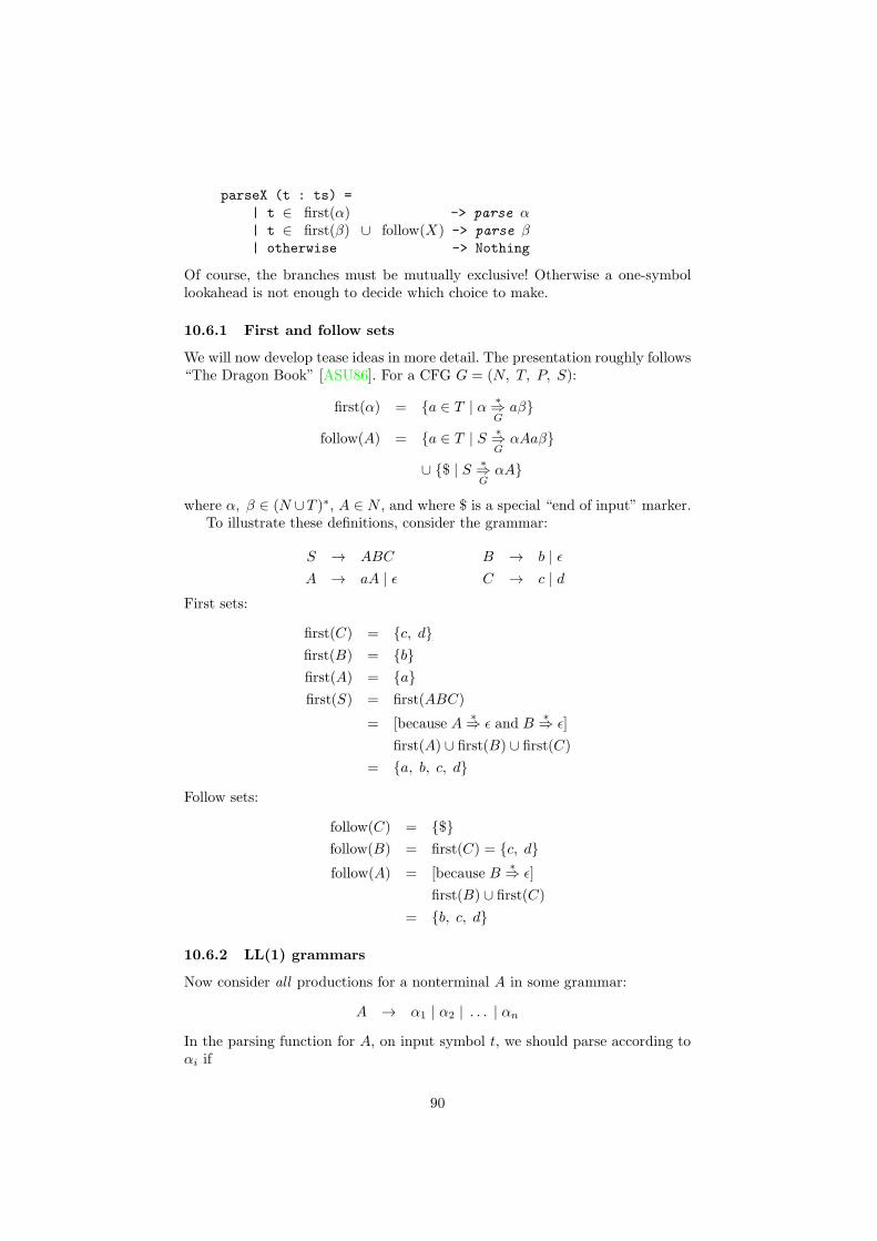
parseX (t : ts) =
| t ∈ first(α) -> parse α| t ∈ first(β) ∪ follow(X) -> parse β| otherwise -> Nothing
Of course, the branches must be mutually exclusive! Otherwise a one-symbollookahead is not enough to decide which choice to make.
10.6.1 First and follow sets
We will now develop tease ideas in more detail. The presentation roughly follows“The Dragon Book” [ASU86]. For a CFG G = (N, T, P, S):
first(α) = {a ∈ T | α∗⇒G
aβ}
follow(A) = {a ∈ T | S∗⇒G
αAaβ}
∪ {$ | S∗⇒G
αA}
where α, β ∈ (N ∪T )∗, A ∈ N , and where $ is a special “end of input” marker.To illustrate these definitions, consider the grammar:
S → ABC
A → aA | ǫ
B → b | ǫ
C → c | d
First sets:
first(C) = {c, d}
first(B) = {b}
first(A) = {a}
first(S) = first(ABC)
= [because A∗⇒ ǫ and B
∗⇒ ǫ]
first(A) ∪ first(B) ∪ first(C)
= {a, b, c, d}
Follow sets:
follow(C) = {$}
follow(B) = first(C) = {c, d}
follow(A) = [because B∗⇒ ǫ]
first(B) ∪ first(C)
= {b, c, d}
10.6.2 LL(1) grammars
Now consider all productions for a nonterminal A in some grammar:
A → α1 | α2 | . . . | αn
In the parsing function for A, on input symbol t, we should parse according toαi if
90

• t ∈ first(αi).
• t ∈ follow(A), if αi∗⇒ ǫ
Thus, if:
• first(αi) ∩ first(αj) = ∅ for 1 ≤ i < j ≤ n, and
• if αi∗⇒ ǫ for some i, then, for all 1 ≤ j ≤ n, j 6= i,
– αj 6∗⇒ ǫ, and
– follow(A) ∩ first(αj) = ∅
then it is always clear what do do! A grammar satisfying these conditions is saidto be an LL(1) grammar.
10.6.3 Nullable nonterminals
In order to compute the first and follow sets for a grammar G = (N, T, P, S),
we first need to know all nonterminals A ∈ N such that A∗⇒ ǫ; i.e. the set
Nǫ ⊆ N of nullable nonterminals.Let syms(α) denote the set of symbols in a string α:
syms ∈ (N ∪ T )∗ → P(N ∪ T )
syms(ǫ) = ∅
syms(Xα) = {X} ∪ syms(α)
The set Nǫ is the smallest solution to the equation
Nǫ = {A | A → α ∈ P ∧ ∀X ∈ syms(α) . X ∈ Nǫ}
(Note that A ∈ Nǫ if A → ǫ ∈ P because syms(ǫ) = ∅ and ∀X ∈ ∅ . . . . istrivially true.)
We can now define a predicate nullable on strings of grammar symbols:
nullable ∈ (N ∪ T )∗ → Bool
nullable(ǫ) = true
nullable(Xα) = X ∈ Nǫ ∧ nullable(α)
The equation for Nǫ can be solved iteratively as follows:
1. Initialize Nǫ to {A | A → ǫ ∈ P}.
2. If there is a production A → α such that ∀X ∈ syms(α) . X ∈ Nǫ, thenadd A to Nǫ.
3. Repeat step 2 until no further nullable nonterminals can be found.
Consider the following grammar:
S → ABC | AB
A → aA | BB
B → b | ǫ
C → c | d
91

• Because B → ǫ is a production, B ∈ Nǫ.
• Because A → BB is a production and B ∈ Nǫ, additionally A ∈ Nǫ.
• Because S → AB is a production, and A,B ∈ Nǫ, additionally S ∈ Nǫ.
• No more production with nullable RHSs. The set of nullable symbols Nǫ ={S,A,B}.
10.6.4 Computing first sets
For a CFG G = (N, T, P, S), the sets first(A) for A ∈ N are the smallest setssatisfying:
first(A) ⊆ T
first(A) =⋃
A→α ∈ P
first(α)
For strings, first is defined as (note the overloaded notation):
first ∈ (N ∪ T )∗ → P(T )
first(ǫ) = ∅
first(aα) = {a}
first(Aα) = first(A) ∪
{
first(α), if A ∈ Nǫ
∅, if A /∈ Nǫ
where a ∈ T , A ∈ N , and α ∈ (N ∪ T )∗.The solutions can often be obtained directly by expanding out all definitions.
If necessary, the equations can be solved by iteration in a similar way to howNǫ is computed. Note that the smallest solution to a set equation of the typeX = X ∪ Y when there are no other constraints on X is simply X = Y .
Consider (again):
S → ABC
A → aA | ǫ
B → b | ǫ
C → c | d
First compute the nullable nonterminals: Nǫ = {A,B}. Then the first sets:
first(A) = first(aA) ∪ first(ǫ)
= {a} ∪ ∅ = {a}
first(B) = first(b) ∪ first(ǫ)
= {b} ∪ ∅ = {b}
first(C) = first(c) ∪ first(d)
= {c} ∪ {d} = {c, d}
first(S) = first(ABC)
= [A ∈ Nǫ]
first(A) ∪ first(BC)
= [B ∈ Nǫ ∧ C /∈ Nǫ]
first(A) ∪ first(B) ∪ first(C) ∪ ∅
= {a} ∪ {b} ∪ {c, d} = {a, b, c, d}
92

10.6.5 Computing follow sets
For a CFG G = (N, T, P, S), the sets follow(A) are the smallest sets satisfying:
• {$} ⊆ follow(S)
• If A → αBβ ∈ P , then first(β) ⊆ follow(B)
• If A → αBβ ∈ P , and nullable(β) then follow(A) ⊆ follow(B)
A,B ∈ N , and α, β ∈ (N ∪ T )∗.(It is assumed that there are no useless symbols; i.e., all symbols can appear inthe derivation of some sentence.)
Here is our example grammar again:
S → ABC
A → aA | ǫ
B → b | ǫ
C → c | d
Constraints for follow(S):
{$} ⊆ follow(S)
Constraints for follow(A) (note: ¬nullable(BC)):
first(BC) ⊆ follow(A)
first(ǫ) ⊆ follow(A)
follow(A) ⊆ follow(A)
Constraints for follow(B) (note: ¬nullable(C)):
first(C) ⊆ follow(B)
Constraints for follow(C) (note: nullable(ǫ)):
first(ǫ) ⊆ follow(C)
follow(S) ⊆ follow(C)
In general:
X ⊆ Z ∧ Y ⊆ Z ⇐⇒ X ∪ Y ⊆ Z
Also, constraints like ∅ ⊆ X and X ⊆ X are trivially satisfied and can beomitted.
The constraints for our example can thus be written as:
{$} ⊆ follow(S)
first(BC) ∪ first(ǫ) ⊆ follow(A)
first(C) ⊆ follow(B)
first(ǫ) ∪ follow(S) ⊆ follow(C)
Using
first(ǫ) = ∅
first(C) = {c, d}
first(BC) = first(B) ∪ first(C) ∪ ∅
= {b} ∪ {c, d} = {b, c, d}
93

the constraints can be simplified further:
{$} ⊆ follow(S)
{b, c, d} ⊆ follow(A)
{c, d} ⊆ follow(B)
follow(S) ⊆ follow(C)
Finally, looking for the smallest sets satisfying these constraints, we get:
follow(S) = {$}
follow(A) = {b, c, d}
follow(B) = {c, d}
follow(C) = follow(S) = {$}
10.6.6 Implementing a predictive parser
Let us now implement a predictive parser for our sample grammar:
S → ABC
A → aA | ǫ
B → b | ǫ
C → c | d
For this grammar, as per the calculations above:
• Nullable symbols: Nǫ = {S,A,B}
• First sets:
first(S) = {a, b, c, d}
first(A) = {a}
first(B) = {b}
first(C) = {c, d}
• Follow sets:
follow(S) = {$}
follow(A) = {b, c, d}
follow(B) = {c, d}
follow(C) = {$}
Recall the “template code” for a parsing function for a pair of productionslike X → α | β. If no RHS is nullable:
parseX (t : ts) =
| t ∈ first(α) -> parse α| t ∈ first(β) -> parse β| otherwise -> Nothing
If one RHS is nullable, say nullable(β):
94
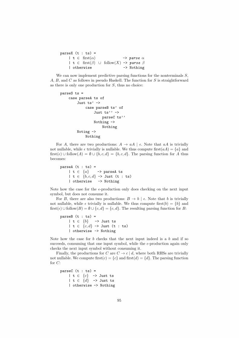
parseX (t : ts) =
| t ∈ first(α) -> parse α| t ∈ first(β) ∪ follow(X) -> parse β| otherwise -> Nothing
We can now implement predictive parsing functions for the nonterminals S,A, B, and C as follows in pseudo Haskell. The function for S is straightforwardas there is only one production for S, thus no choice:
parseS ts =
case parseA ts of
Just ts’ ->
case parseB ts’ of
Just ts’’ ->
parseC ts’’
Nothing ->
Nothing
Noting ->
Nothing
For A, there are two productions: A → aA | ǫ. Note that aA is triviallynot nullable, while ǫ trivially is nullable. We thus compute first(aA) = {a} andfirst(ǫ) ∪ follow(A) = ∅ ∪ {b, c, d} = {b, c, d}. The parsing function for A thusbecomes:
parseA (t : ts) =
| t ∈ {a} -> parseA ts
| t ∈ {b, c, d} -> Just (t : ts)
| otherwise -> Nothing
Note how the case for the ǫ-production only does checking on the next inputsymbol, but does not consume it.
For B, there are also two productions: B → b | ǫ. Note that b is triviallynot nullable, while ǫ trivially is nullable. We thus compute first(b) = {b} andfirst(ǫ) ∪ follow(B) = ∅ ∪ {c, d} = {c, d}. The resulting parsing function for B:
parseB (t : ts) =
| t ∈ {b} -> Just ts
| t ∈ {c, d} -> Just (t : ts)
| otherwise -> Nothing
Note how the case for b checks that the next input indeed is a b and if sosucceeds, consuming that one input symbol, while the ǫ-production again onlychecks the next input symbol without consuming it.
Finally, the productions for C are C → c | d, where both RHSs are triviallynot nullable. We compute first(c) = {c} and first(d) = {d}. The parsing functionfor C:
parseC (t : ts) =
| t ∈ {c} -> Just ts
| t ∈ {d} -> Just ts
| otherwise -> Nothing
95

This can of course be simplified a little, which is the case whenever there aremultiple productions with the RHSs being a single terminal:
parseC (t : ts) =
| t ∈ {c, d} -> Just ts
| otherwise -> Nothing
10.6.7 LL(1), left-recursion, and ambiguity
As we have seen, the LL(1) conditions impose a number of restrictions on agrammar. In particular, no left-recursive or ambiguous grammar can be LL(1)!
Let us prove that a left-recursive grammar cannot be LL(1). Recall that agrammar is left-recursive iff there exists A ∈ N and α ∈ (N ∪ T )∗ such that
A+⇒ Aα (section 8.6). We can assume without loss of generality that there are
no useless symbols and productions in the grammar as any useless productionscan be removed from a grammar without changing the language (section 8.2).
It thus follows that a derivation A+⇒ w, w ∈ T ∗, must also exist.
Let us assume that all derivations are leftmost. Clearly, Aα 6= w, and thusthere must have been a choice at some point differentiating these two derivations.That is, there must exist some B ∈ N for which there are at least two distinctproductions B → β1 | β2 such that
A∗⇒ Bγ ⇒ β1γ
∗⇒ Aα
andA
∗⇒ Bγ ⇒ β2γ
∗⇒ w
Let us now observe that if there is a derivation α∗⇒ β, then first(α) ⊇
first(β). Let us also observe that if ¬nullable(α), then first(αβ) = first(α), andif nullable(α), then first(αβ) = first(α)∪first(β). (These should really be provedas auxiliary lemmas, but they are fairly obvious.)
Now let us consider β1 and β2. If both nullable(β1) and nullable(β2), thenthat is an immediate violation of the LL(1) conditions, so we need not considerthat case further. Moreover, we can assume w 6= ǫ because if the only terminalstring derivable from A is ǫ, then, under the assumption of no useless produc-tions, it must be the case that both nullable(β1) and nullable(β2) which again
violates the LL(1) conditions. Thus, because A+⇒ w and w 6= ǫ, we have:
first(A) ⊇ first(w) 6= ∅
Suppose ¬nullable(β1) and ¬nullable(β2). Because ¬nullable(β1), β1γ∗⇒
Aα, and first(Aα) ⊇ first(A) by definition, we have:
first(β1) = first(β1γ) ⊇ first(Aα) ⊇ first(A) ⊇ first(w)
Because ¬nullable(β2) and β2γ∗⇒ w, we have:
first(β2) = first(β2γ) ⊇ first(w)
Thusfirst(β1) ∩ first(β2) ⊇ first(w) 6= ∅
96
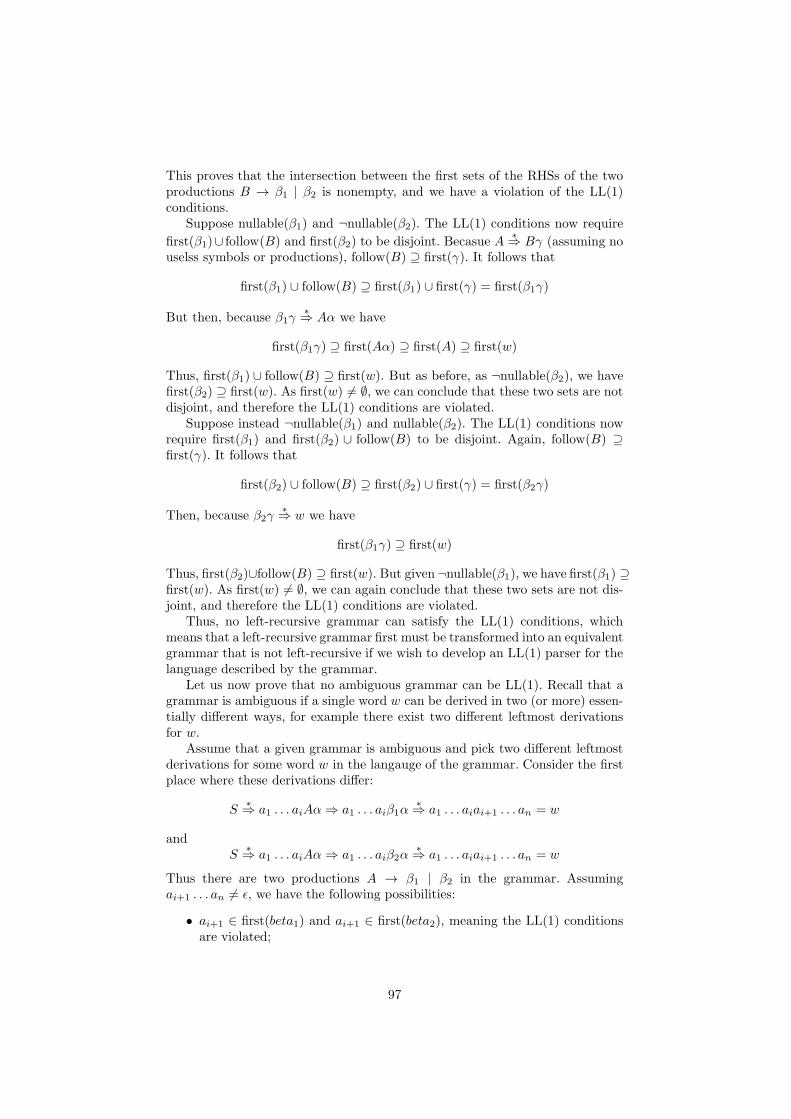
This proves that the intersection between the first sets of the RHSs of the twoproductions B → β1 | β2 is nonempty, and we have a violation of the LL(1)conditions.
Suppose nullable(β1) and ¬nullable(β2). The LL(1) conditions now require
first(β1)∪ follow(B) and first(β2) to be disjoint. Becasue A∗⇒ Bγ (assuming no
uselss symbols or productions), follow(B) ⊇ first(γ). It follows that
first(β1) ∪ follow(B) ⊇ first(β1) ∪ first(γ) = first(β1γ)
But then, because β1γ∗⇒ Aα we have
first(β1γ) ⊇ first(Aα) ⊇ first(A) ⊇ first(w)
Thus, first(β1) ∪ follow(B) ⊇ first(w). But as before, as ¬nullable(β2), we havefirst(β2) ⊇ first(w). As first(w) 6= ∅, we can conclude that these two sets are notdisjoint, and therefore the LL(1) conditions are violated.
Suppose instead ¬nullable(β1) and nullable(β2). The LL(1) conditions nowrequire first(β1) and first(β2) ∪ follow(B) to be disjoint. Again, follow(B) ⊇first(γ). It follows that
first(β2) ∪ follow(B) ⊇ first(β2) ∪ first(γ) = first(β2γ)
Then, because β2γ∗⇒ w we have
first(β1γ) ⊇ first(w)
Thus, first(β2)∪follow(B) ⊇ first(w). But given ¬nullable(β1), we have first(β1) ⊇first(w). As first(w) 6= ∅, we can again conclude that these two sets are not dis-joint, and therefore the LL(1) conditions are violated.
Thus, no left-recursive grammar can satisfy the LL(1) conditions, whichmeans that a left-recursive grammar first must be transformed into an equivalentgrammar that is not left-recursive if we wish to develop an LL(1) parser for thelanguage described by the grammar.
Let us now prove that no ambiguous grammar can be LL(1). Recall that agrammar is ambiguous if a single word w can be derived in two (or more) essen-tially different ways, for example there exist two different leftmost derivationsfor w.
Assume that a given grammar is ambiguous and pick two different leftmostderivations for some word w in the langauge of the grammar. Consider the firstplace where these derivations differ:
S∗⇒ a1 . . . aiAα ⇒ a1 . . . aiβ1α
∗⇒ a1 . . . aiai+1 . . . an = w
andS
∗⇒ a1 . . . aiAα ⇒ a1 . . . aiβ2α
∗⇒ a1 . . . aiai+1 . . . an = w
Thus there are two productions A → β1 | β2 in the grammar. Assumingai+1 . . . an 6= ǫ, we have the following possibilities:
• ai+1 ∈ first(beta1) and ai+1 ∈ first(beta2), meaning the LL(1) conditionsare violated;
97

• One of β1 or β2 derives ǫ, implying ai+1 ∈ follow(A) and ai+1 ∈ first(beta1)or ai+1 ∈ first(beta2), meaning the LL(1) conditions are violated eitherway;
• Both β1 or β2 derive ǫ, a direct violation of the LL(1) conditions.
Assuming ai+1 . . . an = ǫ, then it must be the case that both β1 and β2 arenullable, which violates the LL(1) conditions.
Thus, no ambiguous grammar can satisfy the LL(1) conditions, which meansthat an ambiguous grammar first must be transformed into an equivalent un-ambiguous grammar if we wish to develop an LL(1) parser for the describedlanguage.
10.6.8 Satisfying the LL(1) conditions
Not all grammars satisfy the LL(1) conditions. If we have such a grammar, andwe wish to develop an LL(1) parser, the grammar first has to be transformed. Inparticular, left-recursion and ambiguity must be eliminated because the LL(1)conditions are necessarily violated otherwise (see section 10.6.7). There is nopoint in computing first and follow sets (for the purpose of constructing a LL(1)parser) before this is done. Of course, transforming a grammar in this way isnot always possible: the grammar may be inherently ambiguous, for example(section 8.5). But often transformation into an equivalent grammar satisfyingthe LL(1) conditions is possible.
Section 8 covered a number of transformations, including ones for eliminatingleft recursion and disambiguating grammars. Sometimes other transformationsare needed. A common problem is the following. Note that the productions arenot left recursive, nor would these rules in isolation make a grammar ambiguousas one of the rules derive a word with the terminal c, and the other one withoutthe terminal c:
S → aXbY | aXbY cZ
This grammar is clearly not suitable for predictive parsing as the first sets forthe RHSs of both productions are the same, {a}. But it is also clear that theproblem in this case is relatively simple: there is a common prefix of the RHSsof the two productions. Thus, we can try to postpone the choice by factoringout the common prefix. That could be enough to satisfy the LL(1) conditions.
Thus, what we need here is left factoring (section 8.4). After left factoring:
S → aXbY S′
S′ → ǫ | cZ
As it turns out, this is now suitable for LL(1) parsing!
10.7 Beyond hand-written parsers: use parser generators
The restriction to LL(1) has a number of disadvantages: In many case a naturalgrammar like has to be changed to satisfy the LL(1) conditions. This may evenbe impossible: some context-free languages cannot be generated by any LL(1)grammar.
98

Luckily, there is a more powerful approach called LR(1). LR(1) is a bottom-up method and was briefly discussed in section 10.2. In particular, in contrastto LL(1), LR(1) can handle both left-recursive and right-recursive grammarswithout modification.
The disadvantage with LR(1) and the related approach LALR(1) (which isslightly less powerful but much more efficient) is that it is very hard to constructLR-parsers by hand. Hence there are automated tools that get the grammar asan input and produce a parser as the output. One of the first of those parsergenerators was YACC for C. Nowadays one can find parser generators for manylanguages such as JAVA CUP for Java [Hud99] and Happy for Haskell [Mar01].
However, there are also very serious tools based on LL(k) parsing technol-ogy, such as ANTLR (ANother Tool for Language Recognition) [Par05], thatovercome some of the problems of basic LL parsing and that provides as muchautomation as any other parser generator tool. It is true that a grammar stillmay have to be changed a little bit to parseable, but that is true for LR parsingtoo. In practice, once one become familiar with a tool, it is not that hard towrite a grammar in such a way so as to avoid the most common pitfalls from theoutset. Additionally, most tools provide mechanics such as declarative specifi-cation of disambiguation rules that allows grammars to be written in a naturalway without worrying too much about the details of the underlying parsingtechnology. Today, when it comes to choosing a tool, the underlying parsingtechnology is probably less important than other factors such as tool quality,supported development languages, feature set, etc.
99

10.8 Exercises
Exercise 10.1
Consider the following Context-Free Grammar (CFG):
S → ABB | BBC | CA
A → aA | ǫ
B → Bb | ǫ
C → cC | d
S, A, B, and C are nonterminals, a, b, c, and d are terminals, and S is the startsymbol.
1. What is the set Nǫ of nullable nonterminals? Provide a brief justification.
2. Systematically compute the first sets for all nonterminals, i.e. first(S),first(A), first(B), and first(C), by setting up and solving the equationsaccording to the definitions of first sets for nonterminals and strings ofgrammar symbols. Show your calculations.
3. Set up the subset constraint system that defines the follow sets for allnonterminals, i.e. follow(S), follow(A), follow(B), and follow(C). Simplifywhere possible using the law
X ⊆ Z ∧ Y ⊆ Z ⇐⇒ X ∪ Y ⊆ Z
and the fact that constraints like ∅ ⊆ X and X ⊆ X are trivially satisfiedand can be omitted.
4. Solve the subset constraint system for the follow sets from the previousquestion by finding the smallest sets satisfying the constraints.
100

11 Turing Machines
A Turing machine (TM) is a generalization of a PDA that uses a tape insteadof a stack. Turing machines are an abstract version of a computer: they havebeen used to define formally what is computable. There are a number of alter-native approaches to formalize the concept of computability (for example, theλ-calculus (section 12), µ-recursive functions, the von Neumann architecture,and so on) but they all turn out to be equivalent. That this is the case for anyreasonable notion of computation is called the Church-Turing Thesis.
On the other side there is a generalization of context-free grammars calledphrase structure grammars or just grammars. Here we allow several symbols onthe left hand side of a production, e.g. we may define the context in which arule is applicable. Languages definable by grammars correspond precisely to theones that may be accepted by a Turing machine and those are called Type-0-languages or the recursively enumerable languages (or semidecidable languages)
Turing machines behave differently from the previous machine classes wehave seen: they may run forever, without stopping. To say that a language isaccepted by a Turing machine means that the TM will stop in an acceptingstate for each word that is in the language. However, if the word is not in thelanguage the Turing machine may stop in a non-accepting state or loop forever.In this case we can never be sure whether the given word is in the language;i.e., the Turing machine doesn’t decide the word problem.
We say that a language is recursive (or decidable), if there is a TM thataccepts it and always stop on any word. There are type-0-languages that arenot recursive; the most famous one is the halting problem. This is the languageof encodings of Turing machines that will always stop.
There is no type of grammars that captures all recursive languages (and fortheoretical reasons there cannot be one). However there is a subset of recursivelanguages, called the context-sensitive languages, that can be characterized bycontext-sensitive grammars. These are grammars where the left-hand side of aproduction is always shorter than the right-hand side. Context-sensitive lan-guages on the other hand correspond to linear bounded TMs, that use only atape whose length can be given by a linear function over the length of the input.
11.1 What is a Turing machine?
A Turing machine M = (Q,Σ,Γ, δ, q0, B, F ) is:
• A finite set Q of states;
• A finite set Σ of symbols (the alphabet);
• A finite set Γ of tape symbols s.t. Σ ⊆ Γ. This is the case because we usethe tape also for the input;
• A transition function
δ ∈ Q× Γ → {stop} ∪Q× Γ× {L,R}
The transition function defines how the machine behaves if is in state qand the symbol on the tape is x. If δ(q, x) = stop then the machine stopsotherwise if δ(q, x) = (q′, y, d) the machines gets into state q′, writes y onthe tape (replacing x) and moves left if d = L or right, if d = R;
101

• An initial state q0 ∈ Q;
• The blank symbol B ∈ Γ but B /∈ Σ. Initially, only a finite section of thetape containing the input is non-blank;
• A set of final states F ⊆ Q.
In [HMU01] the transition function is defined without an explicit option tostop with type δ ∈ Q × Γ → Q × Γ × {L,R}. However, they allow δ to beundefined which corresponds to our function returning stop.
The above defines deterministic Turing machines; for nondeterministic TMsthe type of the transition function is changed to:
δ ∈ Q× Γ → P(Q× Γ× {L,R})
In this case, the transition function returning the empty set plays the role ofstop. As for finite automata (and unlike for PDAs) there is no difference in thestrength of deterministic or nondeterministic TMs.
As for PDAs, we define instantaneous descriptions for Turing machines: ID =Γ∗ ×Q×Γ∗. An element (γL, q, γR) ∈ ID describes a situation where the TM isin state Q, the non-blank portion of the tape on the left of the head is γL andthe non-blank portion of the tape on the right, including the square under thehead, is γR.
We define the next-state relation ⊢M
similarly to PDAs:
1. (γL, q, xγR) ⊢M
(γLy, q′, γR) if δ(q, x) = (q′, y,R)
2. (γLz, q, xγR) ⊢M
(γL, q′, zyγR) if δ(q, x) = (q′, y,L)
3. (ǫ, q, xγR) ⊢M
(ǫ, q′, ByγR) if δ(q, x) = (q′, y,L)
4. (γL, q, ǫ) ⊢M
(γLy, q′, ǫ) if δ(q, B) = (q′, y,R)
5. (γLz, q, ǫ) ⊢M
(γL, q′, zy) if δ(q, B) = (q′, y,L)
6. (ǫ, q, ǫ) ⊢M
(ǫ, q′, By) if δ(q, B) = (q′, y,L)
The cases 3 to 6 are only needed to deal with the situation of having reachedthe end of the non-blank part of the tape.
We say that a TM M accepts a word if it goes into an accepting state; i.e.,the language of a TM is defined as
L(M) = {w ∈ Σ∗ | (ǫ, q0, w)∗
⊢M
(γL, q′, γR) ∧ q′ ∈ F}
That is, the TM stops automatically if it goes into an accepting state. However,it may also stop in a non-accepting state if δ returns stop. In this case the wordis rejected. A TM M decides a language if it accepts it and it never loops (inthe negative case).
To illustrate, we define a TM M that accepts the language
L = {anbncn | n ∈ N}
This is a language that cannot be recognized by a PDA or be defined by a CFG.Let M = (Q,Σ,Γ, δ, q0, B, F ) where
102

Q = {q0, q1, q2, q3, q4, q5, q6}
Σ = {a, b, c}
Γ = Σ ∪ {X, Y, Z, }
q0 = q0
B =
F = {q6}
δ(q0, ) = (q6, ,R)
δ(q0, a) = (q1, X,R)
δ(q1, a) = (q1, a,R)
δ(q1, Y) = (q1, Y,R)
δ(q1, b) = (q2, Y,R)
δ(q2, b) = (q2, b,R)
δ(q2, Z) = (q2, Z,R)
δ(q2, c) = (q3, Z,R)
δ(q3, ) = (q5, ,L)
δ(q3, c) = (q4, c,L)
δ(q4, Z) = (q4, Z,L)
δ(q4, b) = (q4, b,L)
δ(q4, Y) = (q4, Y,L)
δ(q4, a) = (q4, a,L)
δ(q4, X) = (q0, X,R)
δ(q5, Z) = (q5, Z,L)
δ(q5, Y) = (q5, Y,L)
δ(q5, X) = (q6, X,R)
δ(q, x) = stop everywhere else
The machine replaces an a by X (q0) and then looks for the first b replacesit by Y (q1) and looks for the first c and replaces it by a Z (q2). If there aremore c’s left it moves left to the next a (q4) and repeats the cycle. Otherwise itchecks whether there are no a’s and b’s left (q5) and if so goes into an acceptingstate (q6).
Graphically the machine can be represented by the following transitiondiagram, where the edges are labelled by (read-symbol, write-symbol, move-direction):
q0 q1 q2
q3q4 q5 q6
a, X,R
a, a,RY, Y,R
b, Y,R
b, b,RZ, Z,R
c, Z,R
c, c,L , ,L
Z, Z,Lb, b,LY, Y,La, a,L
X, X,R
Z, Z,LY, Y,L
X, X,R
103
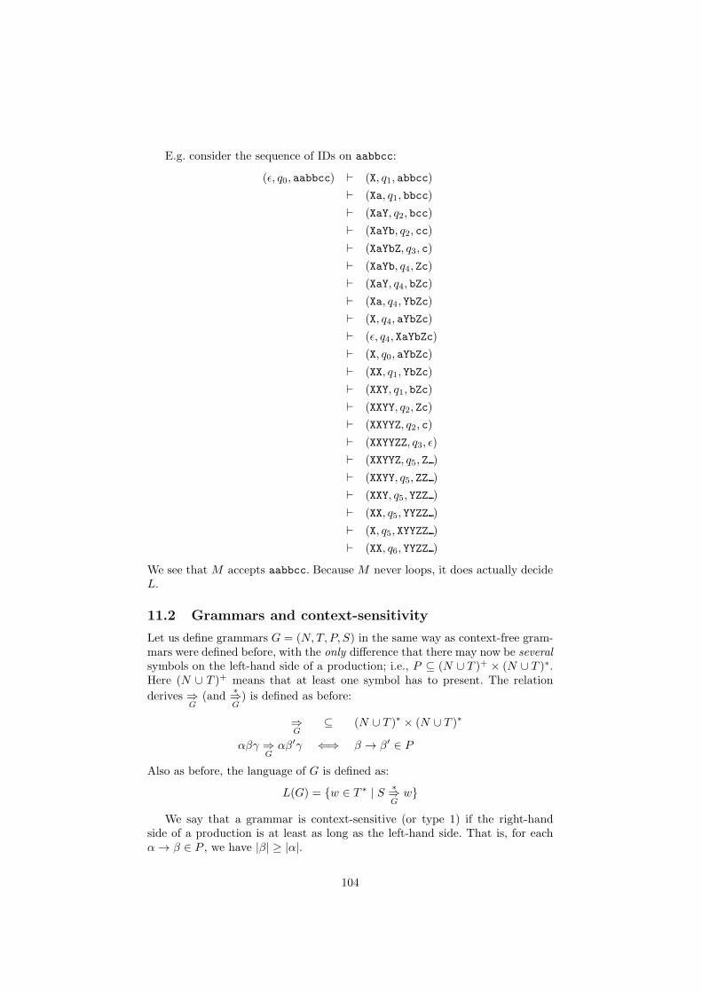
E.g. consider the sequence of IDs on aabbcc:
(ǫ, q0, aabbcc) ⊢ (X, q1, abbcc)
⊢ (Xa, q1, bbcc)
⊢ (XaY, q2, bcc)
⊢ (XaYb, q2, cc)
⊢ (XaYbZ, q3, c)
⊢ (XaYb, q4, Zc)
⊢ (XaY, q4, bZc)
⊢ (Xa, q4, YbZc)
⊢ (X, q4, aYbZc)
⊢ (ǫ, q4, XaYbZc)
⊢ (X, q0, aYbZc)
⊢ (XX, q1, YbZc)
⊢ (XXY, q1, bZc)
⊢ (XXYY, q2, Zc)
⊢ (XXYYZ, q2, c)
⊢ (XXYYZZ, q3, ǫ)
⊢ (XXYYZ, q5, Z )
⊢ (XXYY, q5, ZZ )
⊢ (XXY, q5, YZZ )
⊢ (XX, q5, YYZZ )
⊢ (X, q5, XYYZZ )
⊢ (XX, q6, YYZZ )
We see that M accepts aabbcc. Because M never loops, it does actually decideL.
11.2 Grammars and context-sensitivity
Let us define grammars G = (N, T, P, S) in the same way as context-free gram-mars were defined before, with the only difference that there may now be severalsymbols on the left-hand side of a production; i.e., P ⊆ (N ∪ T )+ × (N ∪ T )∗.Here (N ∪ T )+ means that at least one symbol has to present. The relation
derives ⇒G
(and∗⇒G) is defined as before:
⇒G
⊆ (N ∪ T )∗ × (N ∪ T )∗
αβγ ⇒G
αβ′γ ⇐⇒ β → β′ ∈ P
Also as before, the language of G is defined as:
L(G) = {w ∈ T ∗ | S∗⇒G
w}
We say that a grammar is context-sensitive (or type 1) if the right-handside of a production is at least as long as the left-hand side. That is, for eachα → β ∈ P , we have |β| ≥ |α|.
104
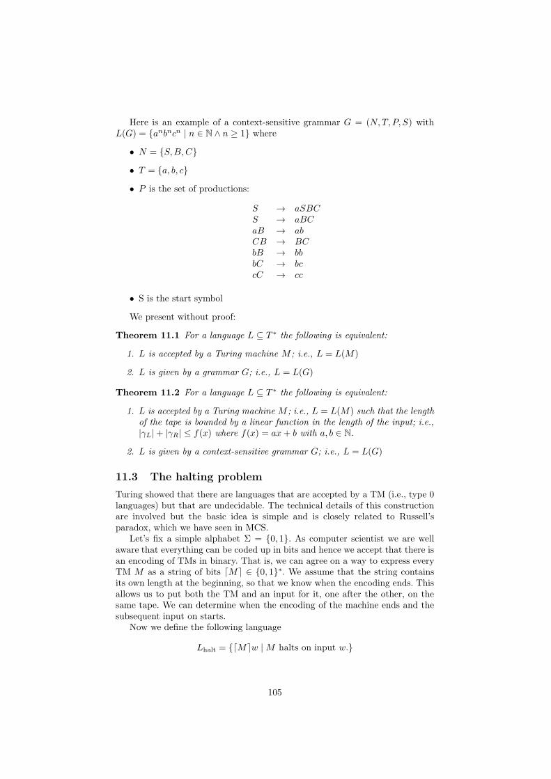
Here is an example of a context-sensitive grammar G = (N, T, P, S) withL(G) = {anbncn | n ∈ N ∧ n ≥ 1} where
• N = {S,B,C}
• T = {a, b, c}
• P is the set of productions:
S → aSBCS → aBCaB → abCB → BCbB → bbbC → bccC → cc
• S is the start symbol
We present without proof:
Theorem 11.1 For a language L ⊆ T ∗ the following is equivalent:
1. L is accepted by a Turing machine M ; i.e., L = L(M)
2. L is given by a grammar G; i.e., L = L(G)
Theorem 11.2 For a language L ⊆ T ∗ the following is equivalent:
1. L is accepted by a Turing machine M ; i.e., L = L(M) such that the lengthof the tape is bounded by a linear function in the length of the input; i.e.,|γL|+ |γR| ≤ f(x) where f(x) = ax+ b with a, b ∈ N.
2. L is given by a context-sensitive grammar G; i.e., L = L(G)
11.3 The halting problem
Turing showed that there are languages that are accepted by a TM (i.e., type 0languages) but that are undecidable. The technical details of this constructionare involved but the basic idea is simple and is closely related to Russell’sparadox, which we have seen in MCS.
Let’s fix a simple alphabet Σ = {0, 1}. As computer scientist we are wellaware that everything can be coded up in bits and hence we accept that there isan encoding of TMs in binary. That is, we can agree on a way to express everyTM M as a string of bits ⌈M⌉ ∈ {0, 1}∗. We assume that the string containsits own length at the beginning, so that we know when the encoding ends. Thisallows us to put both the TM and an input for it, one after the other, on thesame tape. We can determine when the encoding of the machine ends and thesubsequent input on starts.
Now we define the following language
Lhalt = {⌈M⌉w | M halts on input w.}
105

It is easy (although the details are quite daunting) to define a TM that acceptsthis language: we just simulate M and accept if M stops. However, Turingshowed that there is no TM that decides this language.
Let us prove this by assuming that the language is decidable and deriving acontradiction from it. Suppose there is a TM H that decides L. That is, whenrun on a word v, H always terminates and the final state is accepting if andonly if v has the form v = ⌈M⌉w for some machine M and input w and when Mis run on w it terminates. In all other cases, if v is in such form but M does notterminate on w or if v is not in that form at all, H will terminate in a rejectingstate.
Now using H we construct a new TM F that is a bit obnoxious. When werun F on input x, it computes H on the duplicated input xx. If H says yes (itaccepts xx), then F goes into an infinite loop; otherwise, if H says no (it rejectsxx), F stops.
What happens if we run F on its own code ⌈F ⌉? Will it terminate or loopforever? If we consider each of the two possibilities, we get the contradictoryconclusion that the opposite should be true: if we assume that it terminates, wecan prove that it must loop; if we assume that it loops, we can prove that itmust terminate!
Let us assume F on ⌈F ⌉ terminates. By definition of F , this happens onlyif H applied to ⌈F ⌉⌈F ⌉ says no. But by definition of H , this means that F on⌈F ⌉ loops, contradicting the assumption.
Let us then assume that F on input ⌈F ⌉ loops. This happens only if Happlied to ⌈F ⌉⌈F ⌉ says yes. But this means that F on ⌈F ⌉ terminates, againcontradicting the assumption.
We reach a contradiction on both possible behaviours of F : the machine Fcannot exist. We must conclude that our assumption that there is a TM H thatdecides Lhalt is false. We say Lhalt is undecidable.
We have shown that there is no Turing machine that can decide whetherother Turing machines halt. Is this a specific shortcoming of TMs or a univer-sal limitation of all computing models? Maybe we could find a more powerfulprogramming language that overcomes this problem? It turns out that all com-putational formalisms (i.e., programming languages) that have actually beenimplemented are equal in power and can be simulated by each other. BesideTMs, all modern programming languages, the λ-calculus, µ-recursive functionsand many others were proved to be equivalent.
The statement that all models of computability are equivalent is called theChurch-Turing thesis because it was first formulated by Alonzo Church andAlan Turing in the 1930s. This is discussed further in section 12.6.
11.4 Recursive and recursively enumerable sets
When we work with Turing Machines, there is a distinction between a languagebeing accepted or decided.
A machine M accepts a language L if, whenever we run M on an input w,the computation terminates in an accepting state if and only if w ∈ L. We saythat M decides L if it accepts it and always terminates.
The difference is that a machine that just accepts a language but doesn’tdecide it may run forever on some words that do not belong to the language.
106

If that happens, we have to wait forever to discover whether the word is in thelanguage or not.
Definition 11.3 A language L is recursively enumerable if it is accepted by aTuring Machine.
The terminology comes from a different characterization of such languages.We can define a recursively enumerable set as a collection of values that canbe produced by a total algorithm. Whenever we have a computable functionf : N → A from the natural numbers to some set A, we say that the range ofthe function, U = {a ∈ A | ∃n : N, f(n) = a} is recursively enumerable. We canalso write U = {f(n) | n ∈ N}. The idea is that we can enumerate all elementsof U by computing f(0), f(1), f(2), etc. In the case of languages, the set A isΣ∗. We can prove that being a recursively enumerable subset of Σ∗ is equivalentto be accepted by a Turing Machine.
Definition 11.4 A language L is recursive if there is a Turing machine thataccepts it and always terminate.
In general, a recursive set is a subset of some setA for which we can effectivelydetermine membership. Whenever we have a computable function g : A → Bool
from some set A to Booleans, we say that the preimage of true, {a ∈ A | g(a) =true} is recursive.
Theorem 11.5 A subset U ⊆ A is recursive if and only if both U and itscomplement U are recursively enumerable.
Proof. We won’t see a formal proof using Turing Machines, but I’ll outlinethe idea.
• In one direction, assume that U is recursive. So we have a function g :A → Bool that decides it.
We can construct f : N → A by using some enumeration of all of A (weassume it is computably countable, otherwise it won’t make sense to talkabout algorithms on it). When computing the values of f we keep an indexn; we go through all the elements of A one by one, whenever we find ana such that g(a) = true, we set f(n) = a and we increase n by one, nowlooking for the next element of A satisfying g. In this way we constructan f that generates all elements of U , so we proved that U is recursivelyenumerable.
In a similar way we can show that U is recursively enumerable by system-atically searching for the elements a ∈ A for which g(a) = false.
• In the other direction, assume that both U and U are recursively enumer-able. We must prove that U is recursive.
Saying that U is recursively enumerable means that there is a computablefunction f1 : N → A such that U = {f1(a) | n : N}. Saying that U isalso recursively enumerable means that there is a computable functionf2 : N → A such that U = {f2(a) | n : N}.
From f1 and f2 we can construct a function g : A → Bool that decidesU . For a given element a ∈ A, we can search whether it belongs to U byrunning the two functions f1 and f2 repeatedly in parallel:
107
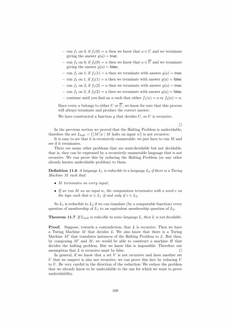
– run f1 on 0, if f1(0) = a then we know that a ∈ U and we terminategiving the answer g(a) = true;
– run f2 on 0, if f2(0) = a then we know that a ∈ U and we terminategiving the answer g(a) = false;
– run f1 on 1, if f1(1) = a then we terminate with answer g(a) = true;
– run f2 on 1, if f2(1) = a then we terminate with answer g(a) = false;
– run f1 on 2, if f1(2) = a then we terminate with answer g(a) = true;
– run f2 on 2, if f2(2) = a then we terminate with answer g(a) = false;
– continue until you find an n such that either f1(n) = a or f2(n) = a.
Since every a belongs to either U or U , we know for sure that this processwill always terminate and produce the correct answer.
We have constructed a function g that decides U , so U is recursive.
�
In the previous section we proved that the Halting Problem is undecidable,therefore the set Lhalt = {⌈M⌉w | M halts on input w} is not recursive.
It is easy to see that it is recursively enumerable: we just have to run M andsee if it terminates.
There are many other problems that are semi-decidable but not decidable,that is, they can be expressed by a recursively enumerable language that is notrecursive. We can prove this by reducing the Halting Problem (or any otheralready known undecidable problem) to them.
Definition 11.6 A language L1 is reducible to a language L2 if there is a TuringMachine M such that:
• M terminates on every input;
• If we run M on an input w, the computation terminates with a word v onthe tape such that w ∈ L1 if and only if v ∈ L2.
So L1 is reducible to L2 if we can translate (by a computable function) everyquestion of membership of L1 to an equivalent membership question of L2.
Theorem 11.7 If Lhalt is reducible to some language L, then L is not decidable.
Proof. Suppose, towards a contradiction, that L is recursive. Then we havea Turing Machine M that decides L. We also know that there is a TuringMachine M ′ that translates instances of the Halting Problem to L. But then,by composing M ′ and M , we would be able to construct a machine H thatdecides the halting problem. But we know this is impossible. Therefore ourassumption that L is recursive must be false. �
In general, if we know that a set V is not recursive and have another setU that we suspect is also not recursive, we can prove this fact by reducing Vto U . Be very careful in the direction of the reduction: We reduce the problemthat we already know to be undecidable to the one for which we want to proveundecidability.
108

11.5 Back to Chomsky
At the end of the course we should have another look at the Chomsky hierarchy,which classifies languages based on sublasses of grammars, or equivalently bydifferent types of automata that recognize them
languages
finite automata
pushdown automata
Type 2 or context free
Type 3 orregular languages
Type 1 or context sensitive languages
Decidable languagesTuring machines
Type 0 or recursively enumerable languages
All languages
We have worked our way from the bottom to the top of the hierarchy: start-ing with finite automata, computation with fixed amount of memory via push-down automata (finite automata with a stack), to Turing machines (finite au-tomata with a tape). Correspondigly we have introduced different grammaticalformalisms: regular expressions, context-free grammars and grammars.
Note that at each level there are languages that are on the next level but noton the previous: {anbn | n ∈ N} is Type 2 but not Type 3, {anbncn} is Type 1but not Type 2, and the Halting problem is Type 0 but not Type 1.
We could have gone the other way: starting with Turing machines and gram-mars and then introducing restrictions: Turing machines that only use theirtapes as a stack describe Type 2 languages; Turing machines that never use thetape apart for reading the input describe Type 3 languages. Similarly, we haveseen that context-free grammars restricted in specific ways describe preciselythe regular languages (section 7.3).
Chomsky introduced his herarchy as a classification of grammars; the rela-tion to automata was only observed a bit later. This may be the reason why heintroduced the Type-1 level, which is not so interesting from an automata pointof view (unless you are into computational complexity; i.e., resource use, herelinear use of memory). It is also the reason why on the other hand the decid-able languages do not constitute a level: there is no corresponding grammaticalformalism (we can even prove this).
109

11.6 Exercises
Exercise 11.1
Consider the Turing Machine defined formally by:
M = (Q,Σ,Γ, δ, q0, , F ) where Q = {q0, q1, q2, q3, q4, q5}F = {q5}Σ = {a, b}Γ = {a, b,X, Y, }
with the transition function defined by:
δ(q0, a) = (q3, X, L)δ(q0, x) = (q0, x, R) for x ∈ {b,X, Y }δ(q0, ) = (q2, , L)δ(q1, b) = (q4, Y, L)δ(q1, x) = (q1, x, R) for x ∈ {a,X, Y }δ(q2, ) = (q5, , R)δ(q2, x) = (q2, x, L) for x ∈ {X,Y }δ(q3, ) = (q1, , R)δ(q3, x) = (q3, x, L) for x ∈ {a, b,X, Y }δ(q4, ) = (q0, , R)δ(q4, x) = (q4, x, L) for x ∈ {a, b,X, Y }
1. Draw M graphically as a transition diagram.
2. Write down the sequence of instantaneous descriptions when starting themachine M with input baab. Is this word accepted or rejected?
3. Write down the sequence of instantaneous descriptions when starting themachine M with input aba. Is this word accepted or rejected?
4. What is the language accepted by M?
Exercise 11.2
Construct a Turing Machine that, when run on any word in {a, b}∗, rear-ranges the symbols so all the as come before all the bs. For example:
(ǫ, q0, aababba) ⊢∗ (aaaabbb, qf , ǫ) (ǫ, q0, babbbaa) ⊢
∗ (aaabbbb, qf , ǫ)
[Hint: Your machine could look for pairs of symbols in the order ‘ba’ and swapthem to ‘ab’; keep repeating this until there are no such pairs left.]
1. Draw the machine as a transition diagram.
2. Give a formal definition of the machine, defining the transition function.
110

Exercise 11.3
Suppose that you have the following information about ten formal problems(expressed as languages) P1, P2, . . . P10:
• The Halting Problem is reducible to P1;
• P2 is reducible to P1;
• P1 is reducible to P5;
• The complement of P3 is recursively enumerable;
• P4 is recursively enumerable;
• P4 is reducible to the normalization problem for λ-calculus;
• P4 is reducible to P5;
• P6 is not recursively enumerable;
• P7 is recursive;
• P7 is reducible to P6;
• P7 is reducible to P8;
• The complement of P8 is not recursively enumerable;
• The normalization problem for λ-calculus is reducible to P9;
• P10 is reducible to P3;
• P10 is reducible to P4.
Note that the normalization problem for λ-calculus (see section 12) is undecid-able Given this information, which of the languages P1 to P10 are:
1. Undecidable?
2. Recursively enumerable?
3. Recursive?
Note that the same language may be in more than one of these three classes.Some others may be in none. Justify your answers by explaining how yourconclusions follow from the given information.
111
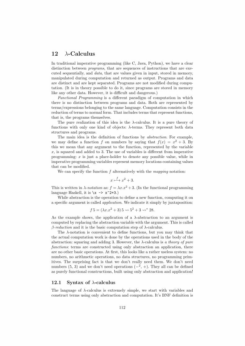
12 λ-Calculus
In traditional imperative programming (like C, Java, Python), we have a cleardistinction between programs, that are sequences of instructions that are exe-cuted sequentially, and data, that are values given in input, stored in memory,manipulated during computation and returned as output. Programs and dataare distinct and are kept separated. Programs are not modified during compu-tation. (It is in theory possible to do it, since programs are stored in memorylike any other data. However, it is difficult and dangerous.)
Functional Programming is a different paradigm of computation in whichthere is no distinction between programs and data. Both are represented byterms/expressions belonging to the same language. Computation consists in thereduction of terms to normal form. That includes terms that represent functions,that is, the programs themselves.
The pure realization of this idea is the λ-calculus. It is a pure theory offunctions with only one kind of objects: λ-terms. They represent both datastructures and programs.
The main idea is the definition of functions by abstraction. For example,we may define a function f on numbers by saying that f(x) = x2 + 3. Bythis we mean that any argument to the function, represented by the variablex, is squared and added to 3. The use of variables is different from imperativeprogramming: x is just a place-holder to denote any possible value, while inimperative programming variables represent memory locations containing valuesthat can be modified.
We can specify the function f alternatively with the mapping notation:
xf
7−→ x2 + 3.
This is written in λ-notation as: f = λx.x2 +3. (In the functional programminglanguage Haskell, it is \x -> x^2+3.)
While abstraction is the operation to define a new function, computing it ona specific argument is called application. We indicate it simply by juxtaposition:
f 5 = (λx.x2 + 3) 5 52 + 3 ∗ 28.
As the example shows, the application of a λ-abstraction to an argument iscomputed by replacing the abstraction variable with the argument. This is calledβ-reduction and it is the basic computation step of λ-calculus.
The λ-notation is convenient to define functions, but you may think thatthe actual computation work is done by the operations used in the body of theabstraction: squaring and adding 3. However, the λ-calculus is a theory of purefunctions: terms are constructed using only abstraction an application, thereare no other basic operations. At first, this looks like a rather useless system: nonumbers, no arithmetic operations, no data structures, no programming prim-itives. The surprising fact is that we don’t really need them. We don’t neednumbers (5, 3) and we don’t need operations (−2, +). They all can be definedas purely functional constructions, built using only abstraction and application!
12.1 Syntax of λ-calculus
The language of λ-calculus is extremely simple, we start with variables andconstruct terms using only abstraction and computation. It’s BNF definition is
112

as follows (assume x, y, z range over a given infinite set of variable names).
t := x | y | z | · · · variable names| λx.t abstraction| t t application.
The β-reduction relation on term is defined, for every pair of terms t1 and t2 as:
(λx.t1) t2 β t1[x := t2].
The left-hand side means: in t1 substitute all occurrences of variable x withthe term t2. Substitution is actually quite tricky and its precise definition is abit more complex that replacing every occurrences of x with t2. One has to becareful to manage variable occurrences properly.
We need some intermediate concept. The first is α-equivalence and it saysthat, since the variable in an abstraction is just a place holder for an argument,the names of abstracted variables does not matter. For example, the simplestfunction we can define is the identity id := λx.x which takes an argument x andreturns it unchanged. Clearly, if we use a different variable name, λy.y, we getexactly the same function. We say that the two terms (and any using differentvariables) are α-equivalent:
λx.x =α λy.y =α λz.z =α · · · .
We are free to change the name of the abstracted variable any way we like.However, we have to be careful to avoid variable capture. If the body of theabstraction contains other variables than the abstracted one, we can’t changethe name to those:
λx.y (x z) =α λw.y (w z) 6=α λy.y (y z) 6=α λz.y (z z).
The reason for this restriction is that changing the name of the abstractedvariable from x to either y or z in this example would capture the occurrence ofthat variable which was free in the original term (not bound by a λ-abstraction).
Formally, we define set FV(t) of the variables that occur free in the term t,by recursion on the structure of t:
FV(x) = {x}FV(λx.t) = FV(t) \ {x}FV(t1 t2) = FV(t1) ∪ FV(t2).
Another way in which a variable can be incorrectly captured is when weperform a substitution that puts a term under an abstraction that may bindsome of its variables:
(λx.λy.x y) (y z) β (λy.x y)[x := (y z)] 6= λy.(y z) y.
If we replace x with (y z) in this way, the occurrence of the variable y (whichwas free before performing the β-reduction) become bound. This is incorrect.We should rename the abstraction variable before performing the substitution:
(λy.x y)[x := (y z)] =α (λw.xw)[x := (y z)] = λw.(y z)w.
113

To avoid problems with variable capture, we adopt the Barendregt variableconvention: before performing substitution (or any other operation on terms),change the names of the abstracted variables so they are different from the freevariables and from each other.
With this convention, we can give a precise definition of substitution byrecursion on the structure of terms:
x[x := t2] = t2y[x := t2] = y if y 6= x
(λy.t1)[x := t2] = λy.t1[x := t2](t0 t1)[x := t2] = t0[x := t2] t1[x := t2].
In the third case, the variable convention ensures that the variable y and thebound variables in t2 have already been renamed so they avoid captures. Inmore traditional formulations, one would add the requirements: “provided thaty 6= x and y doesn’t occur free in t2”.
A part from some complication about substitution, the λ-calculus is ex-tremely simple. It seems at first surprising that we can actually do any seriouscomputation with it at all. But it turns out that all computable functions canbe represented by λ-terms. We see some simple function in this section and wewill discover how to represent data structures in the next.
For convenience, we use some conventions that allow us to save on paren-theses.
• λ-abstraction associates to the right, so we write λx.λy.x for λx.(λy.x);
• Application associates to the left, so we write (t1 t2 t3) for ((t1 t2) t3);
• We can use a single λ symbol followed by several variables to mean con-secutive abstractions, so we write λx y.x for λx.λy.x.
Here are three very simple functions implemented as λ-terms:
• The identity function id := λx.x. When applied to an argument it simplyreturns it unchanged:
id t = (λx.x) t x[x := t] = t.
• The first projection function λx.λy.x. When applied to two arguments, itreturns the first:
(λx.λy.x) t1 t2 (λy.x)[x := t1] t2 = (λy.t1) t2 t1[y := t2] = t1.
Remember, in reading this reduction sequence, that we are adopting thevariable convention, so the variable y doesn’t occur free in t1.
• The second projection function λx.λy.x. When applied to two arguments,it returns the second:
(λx.λy.y) t1 t2 (λy.y)[x := t1] t2 = (λy.y) t2 y[y := t2] = t2.
We can also say that the second projection is the function that, whenapplied to an argument t1, returns the identity function λy.y.
114

12.2 Church numerals
So far we have seen only some very basic functions that only return some oftheir arguments unchanged. How can we define more interesting computations?And first of all, how can we represent values and data structures? It is in factpossible to represent any kind of data buy some λ-term.
Let’s start by representing natural numbers. Their encodings in λ-calculusare called Church Numerals:
0 := λf.λx.x1 := λf.λx.f x2 := λf.λx.f (f x)3 := λf.λx.f (f (f x))· · · .
A numeral n is a function that takes two arguments, denoted by the variablesf and x, and applies f sequentially n times to x.
What is important is that we assign to every number a distinct λ-term in auniform way. We must choose our representation so it is easy to represent arith-metic operations. The idea of Church numerals is nicely conceptual: numbersare objects that we use to count things, so we can define them as the countersof repeated application of a function.
Let’s see if this representation is convenient from the programming point ofview: can we define basic operations on it?
Let’s start with the successor function, that increases a number by one:
succ := λn.λf.λx.f (n f x).
Let’s test if it works on an example: if we apply it to 2 we should get 3:
succ 2 = (λn.λf.λx.f (n f x)) 2 λf.λx.f (2 f x) = λf.λx.f ((λf.λx.f (f x)) f x) λf.λx.f ((λx.f (f x))[f := f ]x) = λf.λx.f ((λx.f (f x))x) λf.λx.f ((f (f x))[x := x]) = λf.λx.f (f (f x)) = 3.
We have explicitly marked the substitutions in this reduction sequence: they areboth trivial, substituting f with itself and x with itself. From now on, we’ll dothe substitutions on the fly, without marking them.
Other arithmetic operations can be defined by simple terms:
plus := λm.λn.λf.λx.m f (n f x)mult := λm.λn.λf.m (n f)exp := λm.λn.nm.
Verify by yourself that these terms correctly implement the addition, multipli-cation and exponentiation functions. For example:
plus 2 3 ∗ 5mult 2 3 ∗ 6exp 2 3 ∗ 8exp 2 3 ∗ 9.
115
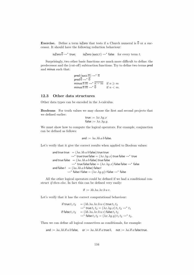
Exercise. Define a term isZero that tests if a Church numeral is 0 or a suc-cessor. It should have the following reduction behaviour:
isZero 0 ∗ true; isZero (succ t) ∗ false for every term t.
Surprisingly, two other basic functions are much more difficult to define: thepredecessor and the (cut-off) subtraction functions. Try to define two terms predand minus such that:
pred (succn) ∗ npred 0 ∗ 0minusnm ∗ n−m if n ≥ mminusnm ∗ 0 if n < m.
12.3 Other data structures
Other data types can be encoded in the λ-calculus.
Booleans For truth values we may choose the first and second projects thatwe defined earlier:
true := λx.λy.xfalse := λx.λy.y.
We must show how to compute the logical operators. For example, conjunctioncan be defined as follows:
and := λa.λb.a b false.
Let’s verify that it give the correct results when applied to Boolean values:
and true true = (λa.λb.a b false) true true
∗ true true false = (λx.λy.x) true false ∗ true
and true false = (λa.λb.a b false) true false
∗ true false false = (λx.λy.x) false false ∗ false
and false t = (λa.λb.a b false) false t
∗ false t false = (λx.λy.y) t false ∗ false
All the other logical operators could be defined if we had a conditional con-struct if-then-else. In fact this can be defined very easily:
if := λb.λu.λv.b u v.
Let’s verify that it has the correct computational behaviour:
if true t1 t2 = (λb.λu.λv.b u v) true t1 t2
∗ true t1 t2 = (λx.λy.x) t1 t2 ∗ t1
if false t1 t2 = (λb.λu.λv.b u v) false t1 t2
∗ false t1 t2 = (λx.λy.y) t1 t2 ∗ t2.
Then we can define all logical connectives as conditionals, for example:
and := λa.λb.if a b false, or := λa.λb.if a true b, not := λa.if a false true.
116

As a curiosity (just a feature of the encoding, don’t read anything deeplyphilosophical in it) notice that false is the true identity!
true id false
This is also a good example in the managing of variables: true = λx.λy.x andid = λx.x. If we follow the variable convention, we shouldn’t use x twice, so let’srename it in the identity: id = λz.z. Then
true id = (λx.λy.x) (λz.z) λy.λz.z = λx.λy.y = false
where at the end we’re free to rename the bound variables according to α-conversion.
Tuples Pairs of λ-terms can be encoded by a single term: If t1 and t2 areterms, we define the encoding of the pair as
〈t1, t2〉 := λx.x t1 t2.
First and second projections are obtained by applying a pair to the familiarprojections (or truth values) that we have already seen:
fst p = p (λx.λy.x)snd p = p (λx.λy.y)
We can verify that they have the correct reduction behaviour:
fst 〈t1, t2〉 = 〈t1, t2〉 (λx.λy.x) = (λx.x t1 t2) (λx.λy.x) (λx.λy.x) t1 t2 ∗ t1,
snd 〈t1, t2〉 = 〈t1, t2〉 (λx.λy.y) = (λx.x t1 t2) (λx.λy.y) (λx.λy.y) t1 t2 ∗ t2.
Triples and longer tuples may be encoded as repeated pairs, for exam-ple 〈t1, t2, t3〉 := 〈t1, 〈t2, t3〉〉, or directly using the same idea as for pairs:〈t1, t2, t3〉 := λx.x t1 t2 t3.
12.4 Confluence
A λ-term may contain several redexes. We have the choice of which one to reducefirst. When we make one step of β-reduction, some of the redexes that were therein the beginning may disappear, some may be duplicated into many copies, somenew ones may be created. Although we say that β-reduction is a “simplification”of the term, in the sense that we eliminate a pair of consecutive abstraction andapplication by immediately performing the associated substitution, the resultingreduced term is not always simpler. It may actually be much longer and morecomplicated.
Therefore it is not obvious that, if we choose different redexes to simplify,we will eventually get the same result. It is also not clear whether the reductionof a term will eventually terminate.
The first property is anyway true. But there are indeed terms whose reduc-tion does not terminate.
Theorem 12.1 (Confluence) Given any λ-term t, if t1 and t2 are two reductsof it, that is t ∗ t1 and t ∗ t2; then there exists a common reduct t3 suchthat t1
∗ t3 and t2 ∗ t3.
117
Proof. TO BE COMPLETED �
Definition 12.2 A normal form is a λ-term that doesn’t contain any redexes.A term weakly normalizes if there is a sequence of reduction steps that ends ina normal form. A term strongly normalizes if any sequence of reduction stepseventually ends in a normal form.
There exist terms that do not normalize. The most famous one is a veryshort expression that reduces to itself:
ω := (λx.x x) (λx.x x) (xx)[x := λx.x x] = (λx.x x) (λx.x x) = ω ω · · · .
There are also terms that grow without bound when we reduce them, for exam-ple:
(λx.x xx) (λx.x xx) (λx.x xx) (λx.x xx) (λx.x xx) (λx.x xx) (λx.x xx) (λx.x xx) (λx.x xx) · · · .
Here is an example of a term that weakly normalizes but doesn’t stronglynormalize:
(λx.λy.x) (λz.z)ω.
This terms applies the first projection function to to arguments. If we immedi-ately reduce the application of the projection, the argument ω disappear andwe are left with the identity function, which is a normal form:
(λx.λy.x) (λz.z)ω λz.z.
However, if we try to reduce the redex inside the second argument, we don’tmake any progress and we could continue reducing it forever.
12.5 Recursion
We have seen how to define some basic arithmetic functions as λ-terms: additionplus, multiplication mult, exponentiation exp. With a little effort you may be ableto define the predecessor function and subtraction. what about (whole) division,maybe using the Euclid algorithm?
If we want to use the λ-calculus as a complete programming language, thereshould be a way to define any computable function. This is indeed possible.In fact there is a single λ-term, called the Y combinator, that allows us to useunrestricted recursion:
Y := λf.(λx.f (xx)) (λx.f (xx)).
This definition is inspired by the non-normalizing term ω. In fact we have thatY id ∗ ω.
The most striking property of Y is that it computes a fixed point for everyterm F :
YF ∗ F (Y F ).
118

This is not exactly true: to be precise, YF (λx.F (xx)) (λx.F (xx)) =: fixFand fixF
∗ F (fixF ). If we keep reducing, we get an infinite sequence of appli-cations of F :
fixF ∗ F fixF
∗ F (F fixF ) ∗ F (F (F fixF ))
∗ · · ·
To define a recursive function, we just need to encode a single step of it asa term F and then use Y to iterate that step as many times as it is necessaryto get a result.
Here is, for example, the definition of the factorial:
factstep := λf.λn.if (isZeron) 1 (multn (f (predn)))fact := Y factstep.
12.6 The universality of λ-calculus
The λ-calculus was invented to answer the question: “What does it mean that aproblem is effectively solvable?” Up to that point the notion of a question beinganswerable by an precise method was left to intuition. Throughout the historyof mathematics many difficult problems were posed. When someone claimedto have a solution, expert mathematicians would analyze it and come to aninformed option about whether it was correct and precise.
But at the beginning of the 20th century, David Hilbert had formulatedthe challenge of defining exactly what we mean by a precise method: can wegive a mathematically rigorous definition of what an effective procedure is?Both Alonzo Church and Alan Turing worked towards a realization of Hilbert’schallenge and they both came up with a fully satisfying solution.
But their two theories looked completely different. Which one would be the“true” answer to Hilbert’s question? It turned out that, beyond their formaldifference, Turing machines and λ-terms are equally expressive. The same setof computable functions can be implemented in both. Turing himself provedthis when he discovered Church’s work and added a sketch of the proof as anAppendix to his article about computable numbers.
Around the same time, other models of computation were proposed. KurtGodel formulated the notion of µ-recursive function: any function on the naturalnumbers defined by certain forms of recursive definition. Stephen Kleene, astudent of Church, proved that these functions are exactly those definable inthe λ-calculus and went on the develop a rich theory of computation based onthem.
Another of Church’s students, J. Barkley Rosser, was the first to clearlyformulate the notion that these three definitions were equivalent realizations ofthe informal notion of an effective computation method: “All three definitionsare equivalent, so it does not matter which one is used.”
Later, when the first digital computers were constructed, the Hungarian-American mathematician John von Neumann proposed a model that is morerealistic and describes the actual architecture of real computers: the registermachine. This notion was also equivalent to the previous ones. Many otherdifferent characterizations have been proposed since and they all turned out tobe equivalent.
The statement that every effective definition of computable processes isequivalent to the λ-calculus (or to Turing machines or to µ-recursive functions
119

and so on) is known as the Church-Turing Thesis (Stephen Kleene was the onewho actually first formulated and named it).
The λ-calculus is not just a mathematical abstraction. All functional pro-gramming languages are based on (a typed version of) it. Lisp, ML, Haskell,OCaml are the most well-known. Functional programming has been so suc-cessful that traditional imperative languages are starting to introduce functionabstraction as a basic feature in their definition. For example JavaScript andPython contain first-class functions as part of their definition.
12.7 Exercises
Exercise 12.1
Consider the following λ-terms: nand-pair is a function on pairs of Booleans,nand-fun a function from Church Numerals to pairs of Booleans:
nand-pair = λp.〈not (and (p true) (p false)), p true〉nand-fun = λn.n nand-pair 〈false, false〉
1. What values do the following terms reduce to?
nand-pair 〈true, true〉 ∗ ?nand-pair 〈true, false〉 ∗ ?
nand-pair 〈false, true〉 ∗ ?nand-pair 〈false, false〉 ∗ ?
2. Show the steps of reduction in the computation of (nand-fun 4). [You canuse the previous reductions and those from the lecture notes as singlesteps.]
3. Give an informal definition of what nand-fun does: for which numbers ndoes (nand-funn) ∗ 〈true, true〉?
Exercise 12.2
Write a λ-term that implements the following function:
thrFib : N → N
thrFib 0 = 0thrFib 1 = 0thrFib 2 = 1thrFib (n+ 3) = thrFibn+ thrFib (n+ 1) + thrFib (n+ 2)
[Use the same idea that was used in the lecture to define the Fibonacci numbers:first write an auxiliary function that returns a triple of numbers and then extractthe first.]
120

13 Algorithmic Complexity
The undecidability of the Halting Problem shows that there are tasks that areimpossible to accomplish using any computing machine. This is an intrinsiclimitation of computation. But even for some problems for which algorithmicsolutions are known, it may be impossible to compute them effectively. In somecases, the search for a solution is so complex that it would take a time longerthan the age of the universe to get the answer. We can always hope for dramaticimprovements in the power and speed of computers, but some tasks seem to havean essentially intractable complexity.
In talking about the time complexity of algorithms, we want to abstract awayfrom implementation details. The exact number of steps needed to compute aresult may depend on the model of computation: the same algorithm, realizedas a Turing Machine or as a λ-term, will result in different number of headoperations of the machine and reduction steps of the λ-term. The exact timeof the computation will depend on the specific machine on which it runs: eventhe exact same program in the exact same language will take different times ondifferent computers.
But beyond these differing details, the complexity classes of algorithms arequite constant across different models of computation and different comput-ing devices. A complexity class characterizes algorithms that have a relationbetween size of the input and time of computation that can be expressed bycertain functions. Although they are traditionally formulated in terms of Tur-ing Machines, we can show that realizations in different paradigms have similarbehaviour.
The most important complexity classes are P and NP . P stands for Poly-nomial Complexity: A problem is in P if it can be solved by a Turing Machinewhose running time is at most a polynomial in the size of the input. NP standsfor Non-deterministic Polynomial Complexity: A problem is in NP if it can besolved by a Non-deterministic Turing Machine (NTM) whose running time is atmost a polynomial in the size of the input. Remember that an NTM may haveoverlapping transitions: in certain configurations, the machine may have severalallowed steps. In every run, it will randomly choose which transition to apply.A word is accepted if there exists one possible computation (among all allowedby the non-deterministic choices) that reaches an accepting state.
There are two alternative and equivalent ways of seeing the class NP . Aproblem is in NP if it is solvable in polynomial time by a parallel computerwhich is allowed to spawn several parallel computations. Each computation isindependent and must terminate in polynomial time; it is sufficient that thesolution is found by one of the computations. Although the running time ispolynomial, there may be an exponential blow-up of the number of parallelcomputations that need to run simultaneously.
The second alternative explanation of the class NP is that a problem is in itif we can verify solutions in polynomial time. There is an algorithm that, whengiven as input an instance of the problem and a potential solution, terminatesin polynomial time and gives a positive answer if and only if the solution iscorrect.
Intuitively, it seems obvious that a problem that belongs to NP doesn’tnecessarily belong to P : being able to find a solution in polynomial time by usingnon-deterministic or parallel computations, or being able to verify a solution in
121

polynomial time, doesn’t mean that we can generate a solution deterministicallyin polynomial time. There may be an exponential number of non-deterministicor parallel computations and an exponential number of potential solutions toverify.
However, until now nobody managed to prove that P 6= NP . It is themost famous open problem in theoretical computer science. There are strongreasons to believe that the two classes are distinct. There is a subclass of NP ,called NP-complete, that contains problems that are in a sense universal withrespect to this issue. A problem is in NP-complete if it is in NP and everyother problem inNP can be reduced to it in polynomial time. This means that ifsomebody finds a polynomial-time algorithm to solve one of these problems, thenautomatically all NP problems will be solvable in polynomial time. To date,thousands of different problems from disparate branches of computer science andmathematics have been proved to be NP-complete. It seems highly unlikely thatwe could solve them all at once with the same algorithm.
13.1 The Satisfiability Problem
The first problem to be provedNP-complete was Boolean Satisfiability (in shortSAT). An instance of the problem is a propositional formula, that is, an ex-pression that uses variables, the propositional connectives for conjunction (∧),disjunction (∨) and negation (¬), and parentheses. An example is the formula(x1 ∨ ¬x2) ∧ ¬x1.
Solving an instance of SAT means determining if there is an assignment oftruth values to the variables that makes the formula true. In the example abovethe assignment [x1 7→ false, x2 7→ false] is such a solution. Now consider thefollowing more complicated formula in three variables:
f = (¬x1 ∨ x2) ∧ (x3 ∨ ¬x2) ∧ ¬(x3 ∧ ¬x1) ∧ (x1 ∧ ¬x2 ∨ x2 ∧ ¬x3).
There is no assignment of truth values to x1, x2, x3 that makes f true. To checkthis, we must try all potential solutions:
[x1 7→ true, x2 7→ true, x3 7→ true] =⇒ f 7→ false
[x1 7→ true, x2 7→ true, x3 7→ false] =⇒ f 7→ false
[x1 7→ true, x2 7→ false, x3 7→ true] =⇒ f 7→ false
[x1 7→ true, x2 7→ false, x3 7→ false] =⇒ f 7→ false
[x1 7→ false, x2 7→ true, x3 7→ true] =⇒ f 7→ false
[x1 7→ false, x2 7→ true, x3 7→ false] =⇒ f 7→ false
[x1 7→ false, x2 7→ false, x3 7→ true] =⇒ f 7→ false
[x1 7→ false, x2 7→ false, x3 7→ false] =⇒ f 7→ false
In general, to look for a solution or to verify that there is no solution, we needto check all the possible assignments of truth values to the variables. If thereare n variables in the formulas, then we must check 2n assignments. Thereforechecking them all takes a time that is exponential in the number of variables,so exponential in the side of the input. On the other hand, it is straightforwardto verify whether an assignment gives a solution or not.
13.2 Time Complexity
Let’s define time complexity exactly using Turing Machines.
122

Definition 13.1 A Turing Machine M is said to have time complexity f , afunction N → N, if, whenever we run M on an input of size n, it will take atmost f(n) steps to terminate.
The number of steps is measured by counting the movement of the read-ing/writing head of M , as given by the next-state relation ⊢
M.
This is a worst case measure of the running time of the machine: It is possiblethat M will terminate in less than n steps on some (or all) inputs. So f providesjust an upper bound. We are interested in getting the answer within a certaintime constraint.
As we know, any “problem” can be expressed precisely as a language recog-nition task. Each instance of the problem is specified by giving a description inthe form of a word/list of symbols. So defining complexity classes for problemsis the same as defining them for languages.
Definition 13.2 A language L is in the class P if there is a Turing Machine Mthat decides L and has a time complexity expressible by a polynomial function.
In the previous two definitions, we were talking about deterministic Turingmachines. In any given instantaneous description of M , the transition functiondetermines uniquely the step to be performed.
We are also going to consider non-deterministic Turing machines. Thesemay have several possible transitions in the same instantaneous description.The transition function has the type:
δ ∈ Q× Γ → P(Q× Γ× {L,R})
So, if M is in state q and the head is reading a symbol x, the transition δ(q, x) isa set of triples, each one specifying a different action. For example, if δ(q, x) ={(q1, y,L), (q2, z,R)}, then the machine may either write a y, move left and gointo state q1 or write a z, move right and go into state q2. When we run themachine, in these situation it will randomly choose which of the several possiblesteps to perform. We say that such a machine accepts a word if there is one run(among the many possible) that leads to an accepting state.
Definition 13.3 A language L is in the class NP if there is a non-deterministicTuring Machine M that decides L and has a time complexity expressible by apolynomial function. In this case the polynomial bound must apply to all possibleruns of M on a given input word.
Equivalently, we can express membership in the classNP using deterministicTuring machines that take as input both a word and a certificate that provesthat the word belongs to L. A certificate can be any string of symbols that themachine may interpret as evidence.
Theorem 13.4 A language L is in the class NP if there is a deterministicTuring Machine M and a polynomial function f with the following properties:
• When we run M on a tape containing two inputs w and v (separated by ablank), it always terminates in a number of steps smaller than f(|w|);
• If w ∈ L, then there exists some v such that M gives a positive answerwhen run on w and v;
123

• If w /∈ L, then for every v, M always gives a negative answer when runon w and v.
A string v such that M gives a positive answer when run on w and v is acertificate or proof that w is in L. If you think of L as representing some problemand w as an instance of it, then v can be thought of as a solution for w.
For example, given an instance of SAT, a certificate is an assignment oftruth values to the variables that makes the formula true. We can define aTuring Machine with polynomial time complexity that, when run on a formulaand an assignment of values to the variables, determines whether the formulacomputes to true under that assignment.
Theorem 13.5 SAT is in NP.
13.3 NP-completeness
Among the NP problems there are some that are universal in the sense that allNP problems can be reduced to them in polynomial time.
Definition 13.6 A language L0 is in NP-complete if it is NP and, for everylanguage L1 in NP there exists a Turing Machine M that runs in polynomialtime, with the following property:
When we run M on a word w1, it will terminate with the tape containing aworld w0 such that w1 ∈ L1 if and only if w0 ∈ L0.
We say that L1 is reduced to L0 in polynomial time.
Seeing L0 and L1 as encodings of problems P0 and P1, the definition saysthat we can turn every problem of P1 into a problem of P0 with the samesolution.
The great turning point in the study of the time complexity of algorithmscame with the discovery that there exist some NP-complete problems.
Theorem 13.7 (Stephen Cook, 1971) SAT is NP-complete.
Since Cook’s Theorem, many other problems have been shown to be NP-complete. They now run in the thousands. Here’s a brief description of somefamous ones.
The Travelling Salesman A salesman must visit n different towns. He hasa table giving the distances between any pair of towns. He has a budgetthat he can use to buy petrol, which will allow him to travel a maximumlength. Is there a route around all the towns with length shorter or equalto that allowed by the budget?
Subset Sum Given a set of (positive and negative) integers, is there a non-empty subset of it that sums up to zero? This is a special case of theknapsack problem that consists in maximizing the value of a set of objectsthat can fit into a knapsack with a limited capacity.
Graph Colouring Given a graph and a fixed number of colours, is it possibleto colour all the nodes of the graph so that two nodes of the same colourare not linked by an edge?
124

To this day, it is still unknown whether there are NP problems that are notin P . All attempts to find a polynomial algorithm that solves any NP-complete
problem have failed. Also all attempts to prove that such an algorithm doesn’texist have failed.
If we were to discover such an algorithm, it would automatically give us away to solve all NP-complete problems in polynomial time: we can just reducethem all to the one we can solve. For this reason, most mathematicians andcomputer scientists think that it is impossible, but the question is still open andmay be the greatest mystery in computer science:
P = NP ?
13.4 Exercises
Exercise 13.1
This and the next exercise concerns programing a SAT solver in Haskell. Thefirst exercise is to write a program that checks whether a proposed solution toan instance of SAT is correct. Use the following type definitions:
data SAT = Var Int | Not SAT | And SAT SAT | Or SAT SAT
type Assignment = [Bool]
SAT represents Boolean formulas with variables Var 0, Var 1, Var 2, Var 3
and so on. An assignment is a list of Booleans, giving the values to someof the variables. For example [True,False,False,True] assigns the values:Var 0 = True, Var 1 = False, Var 2 = False, Var 3 = True. The other vari-ables are left without value.
Write an evaluation function:
evaluate :: SAT -> Assignment -> Bool
It uses an assignment of values to variables to evaluate a formula. (If the formulacontains variables with indices larger or equal to the length of the assignment,you can leave it undefined.)
Exercise 13.2
This exercise concerns writing a program that decides the solvability of aninstance of SAT. We will break the task down into several steps.
1. Write a function that gives the highest index of a variable occurring in aformula:
varNum :: SAT -> Int
2. Write a function that generates all the assignments for all variables upto a given index:
allAssign :: Int -> [Assignment]
For example allAssign 2 should give all the possible assignments forvariables Var 0, Var 1 and Var 2:
125
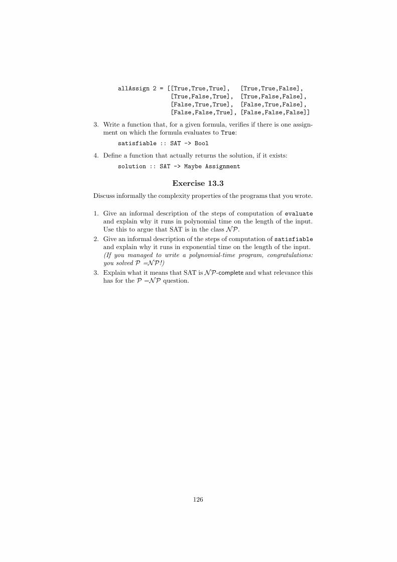
allAssign 2 = [[True,True,True], [True,True,False],
[True,False,True], [True,False,False],
[False,True,True], [False,True,False],
[False,False,True], [False,False,False]]
3. Write a function that, for a given formula, verifies if there is one assign-ment on which the formula evaluates to True:
satisfiable :: SAT -> Bool
4. Define a function that actually returns the solution, if it exists:
solution :: SAT -> Maybe Assignment
Exercise 13.3
Discuss informally the complexity properties of the programs that you wrote.
1. Give an informal description of the steps of computation of evaluateand explain why it runs in polynomial time on the length of the input.Use this to argue that SAT is in the class NP .
2. Give an informal description of the steps of computation of satisfiableand explain why it runs in exponential time on the length of the input.(If you managed to write a polynomial-time program, congratulations:you solved P =NP!)
3. Explain what it means that SAT is NP-complete and what relevance thishas for the P =NP question.
126
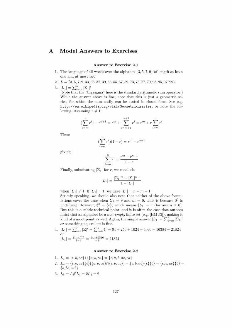
A Model Answers to Exercises
Answer to Exercise 2.1
1. The language of all words over the alphabet {3, 5, 7, 9} of length at leastone and at most two.
2. L = {3, 5, 7, 9, 33, 35, 37, 39, 53, 55, 57, 59, 73, 75, 77, 79, 93, 95, 97, 99}
3. |L1| =∑n
i=m |Σ1|i
(Note that the “big sigma” here is the standard arithmetic sum operator.)While the answer above is fine, note that this is just a geometric se-ries, for which the sum easily can be stated in closed form. See e.g.http://en.wikipedia.org/wiki/Geometric series, or note the fol-lowing. Assuming r 6= 1:
(
n∑
i=m
ri) + rn+1 = rm +
n+1∑
i=m+1
ri = rm + r
n∑
i=m
ri
Thus:
(
n∑
i=m
ri)(1 − r) = rm − rn+1
givingn∑
i=m
ri =rm − rn+1
1− r
Finally, substituting |Σ1| for r, we conclude
|L1| =|Σ1|m − |Σ1|n+1
1− |Σ1|
when |Σ1| 6= 1. If |Σ1| = 1, we have |L1| = n−m+ 1.Strictly speaking, we should also note that neither of the above formu-lations cover the case when Σ1 = ∅ and m = 0. This is because 00 isundefined. However, ∅0 = {ǫ}, which means |L1| = 1 (for any n ≥ 0).But this is a subtle technical point, and it is often the case that authorsinsist that an alphabet be a non-empty finite set (e.g. [HMU3]), making itkind of a moot point as well. Again, the simple answer |L1| =
∑n
i=m |Σ1|i
or something equivalent is fine.
4. |L1| =∑7
i=3 |Σ|i =
∑7i=3 4
i = 64 + 256 + 1024 + 4096 + 16384 = 21824or|L1| =
43−47+1
1−4 = 64−65536−3 = 21824
Answer to Exercise 2.2
1. L3 = {ǫ, b, ac} ∪ {a, b, ca} = {ǫ, a, b, ac, ca}
2. L4 = {ǫ, b, ac}{ǫ}({a, b, ca}∩{ǫ, b, ac}) = {ǫ, b, ac}{ǫ}{b}= {ǫ, b, ac}{b} ={b, bb, acb}
3. L5 = L3∅L4 = ∅L4 = ∅
127
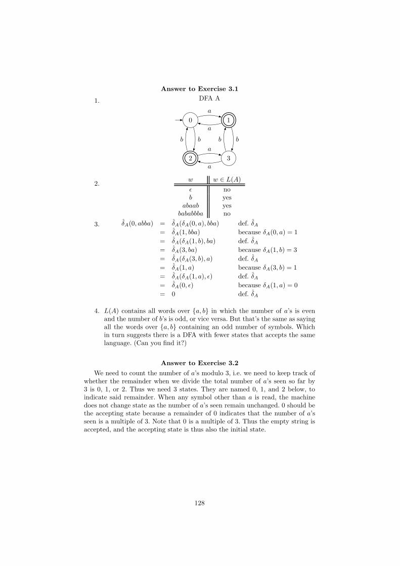
Answer to Exercise 3.1
1. DFA A
0 1
2 3
a
b
a
b
a
b
a
b
2.w w ∈ L(A)
ǫ nob yes
abaab yesbababbba no
3. δA(0, abba) = δA(δA(0, a), bba) def. δA= δA(1, bba) because δA(0, a) = 1
= δA(δA(1, b), ba) def. δA= δA(3, ba) because δA(1, b) = 3
= δA(δA(3, b), a) def. δA= δA(1, a) because δA(3, b) = 1
= δA(δA(1, a), ǫ) def. δA= δA(0, ǫ) because δA(1, a) = 0
= 0 def. δA
4. L(A) contains all words over {a, b} in which the number of a’s is evenand the number of b’s is odd, or vice versa. But that’s the same as sayingall the words over {a, b} containing an odd number of symbols. Whichin turn suggests there is a DFA with fewer states that accepts the samelanguage. (Can you find it?)
Answer to Exercise 3.2
We need to count the number of a’s modulo 3, i.e. we need to keep track ofwhether the remainder when we divide the total number of a’s seen so far by3 is 0, 1, or 2. Thus we need 3 states. They are named 0, 1, and 2 below, toindicate said remainder. When any symbol other than a is read, the machinedoes not change state as the number of a’s seen remain unchanged. 0 should bethe accepting state because a remainder of 0 indicates that the number of a’sseen is a multiple of 3. Note that 0 is a multiple of 3. Thus the empty string isaccepted, and the accepting state is thus also the initial state.
128

0
1
2
a
b, c, d
a
b, c, da
b, c, d
Answer to Exercise 3.3
We need one state for each possible remainder when dividing by 5, i.e. 5states. Let us label each state with the remainder in question. State 0 is thusboth the initial and the only final state. We then just note that if the remainderwhen dividing the sum n of the symbols seen so far by 5 is r, and the nextsymbol is i, then the remainder of n + i divided by 5 is just the remainder ofr + i divided by 5.
0
1
23
4
0
0
00
0
1
1
1
1
12
2
2
2
23
3
33
3
As the question does not specifically ask for a transition diagram, any com-plete representation of a DFA equivalent to the one above is OK:
129
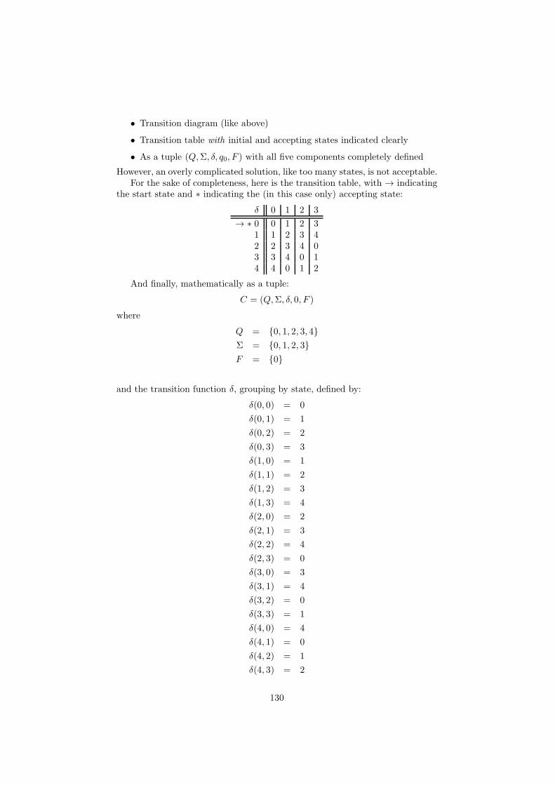
• Transition diagram (like above)
• Transition table with initial and accepting states indicated clearly
• As a tuple (Q,Σ, δ, q0, F ) with all five components completely defined
However, an overly complicated solution, like too many states, is not acceptable.For the sake of completeness, here is the transition table, with → indicating
the start state and ∗ indicating the (in this case only) accepting state:
δ 0 1 2 3
→ ∗ 0 0 1 2 31 1 2 3 42 2 3 4 03 3 4 0 14 4 0 1 2
And finally, mathematically as a tuple:
C = (Q,Σ, δ, 0, F )
where
Q = {0, 1, 2, 3, 4}
Σ = {0, 1, 2, 3}
F = {0}
and the transition function δ, grouping by state, defined by:
δ(0, 0) = 0
δ(0, 1) = 1
δ(0, 2) = 2
δ(0, 3) = 3
δ(1, 0) = 1
δ(1, 1) = 2
δ(1, 2) = 3
δ(1, 3) = 4
δ(2, 0) = 2
δ(2, 1) = 3
δ(2, 2) = 4
δ(2, 3) = 0
δ(3, 0) = 3
δ(3, 1) = 4
δ(3, 2) = 0
δ(3, 3) = 1
δ(4, 0) = 4
δ(4, 1) = 0
δ(4, 2) = 1
δ(4, 3) = 2
130

or, if you prefer to group by input symbols instead:
δ(0, 0) = 0
δ(1, 0) = 1
δ(2, 0) = 2
δ(3, 0) = 3
δ(4, 0) = 4
δ(0, 1) = 1
δ(1, 1) = 2
δ(2, 1) = 3
δ(3, 1) = 4
δ(4, 1) = 0
δ(0, 2) = 2
δ(1, 2) = 3
δ(2, 2) = 4
δ(3, 2) = 0
δ(4, 2) = 1
δ(0, 3) = 3
δ(1, 3) = 4
δ(2, 3) = 0
δ(3, 3) = 1
δ(4, 3) = 2
Answer to Exercise 3.4
1. (a) ǫ ∈ L(A)(b) aaa ∈ L(A)(c) bbc ∈ L(A)(d) cbc /∈ L(A)(e) abcacb ∈ L(A)
2. Starting from SA = {q0, q1, q3}, the start state of D(A), we compute
δA(SA, x) for each x ∈ ΣA. Whenever we encounter a state P ⊆ QA ofD(A) that has not been considered before, we add P to the table and
proceed to tabulate δA(P, x) for each x ∈ ΣA. We repeat the process untilno new states are encountered. Finally, we identify the initial state (→ tothe left of the state) and all accepting states (∗ to the left of the state).Note that a DFA state is accepting iff it contains at least one acceptingNFA state (as this means it is possible to reach at least one acceptingstate on a given word, which means that word is considered to be in thelanguage of the NFA).
131

δD(A) a b c
→ ∗ {q0, q1, q3} {q0, q1, q3} ∪ ∅ ∪ ∅= {q0, q1, q3}
{q0} ∪ {q1} ∪ {q4}= {q0, q1, q4}
{q0} ∪ {q2} ∪ {q3}= {q0, q2, q3}
∗ {q0, q1, q4} {q0, q1, q3} ∪ ∅ ∪ ∅= {q0, q1, q3}
{q0} ∪ {q1} ∪ ∅= {q0, q1}
{q0} ∪ {q2} ∪ ∅= {q0, q2}
∗ {q0, q2, q3} {q0, q1, q3} ∪ ∅ ∪ ∅= {q0, q1, q3}
{q0} ∪ ∅ ∪ {q4}= {q0, q4}
{q0} ∪ ∅ ∪ {q3}= {q0, q3}
∗ {q0, q1} {q0, q1, q3} ∪ ∅= {q0, q1, q3}
{q0} ∪ {q1}= {q0, q1}
{q0} ∪ {q2}= {q0, q2}
∗ {q0, q2} {q0, q1, q3} ∪ ∅= {q0, q1, q3}
{q0} ∪ ∅ = {q0} {q0} ∪ ∅ = {q0}
∗ {q0, q4} {q0, q1, q3} ∪ ∅= {q0, q1, q3}
{q0} ∪ ∅ = {q0} {q0} ∪ ∅ = {q0}
∗ {q0, q3} {q0, q1, q3} ∪ ∅= {q0, q1, q3}
{q0} ∪ {q4}= {q0, q4}
{q0} ∪ {q3}= {q0, q3}
{q0} {q0, q1, q3} {q0} {q0}
(Note that we only needed to consider 8 states, a lot fewer than the25 = 32 possible states in this case. 32 − 8 = 24 states are thus notreachable from the initial state.)Giving simple names to the states resulting from the subset constructioncan facilitate drawing the transition diagram:
δD(A) a b c
→ ∗ {q0, q1, q3} = A {q0, q1, q3} = A {q0, q1, q4} = B {q0, q2, q3} = C∗ {q0, q1, q4} = B {q0, q1, q3} = A {q0, q1} = D {q0, q2} = E∗ {q0, q2, q3} = C {q0, q1, q3} = A {q0, q4} = F {q0, q3} = G∗ {q0, q1} = D {q0, q1, q3} = A {q0, q1} = D {q0, q2} = E∗ {q0, q2} = E {q0, q1, q3} = A {q0} = H {q0} = H∗ {q0, q4} = F {q0, q1, q3} = A {q0} = H {q0} = H∗ {q0, q3} = G {q0, q1, q3} = A {q0, q4} = F {q0, q3} = G
{q0} = H {q0, q1, q3} = A {q0} = H {q0} = H
3. We can now draw the transition diagram for D(A):
132
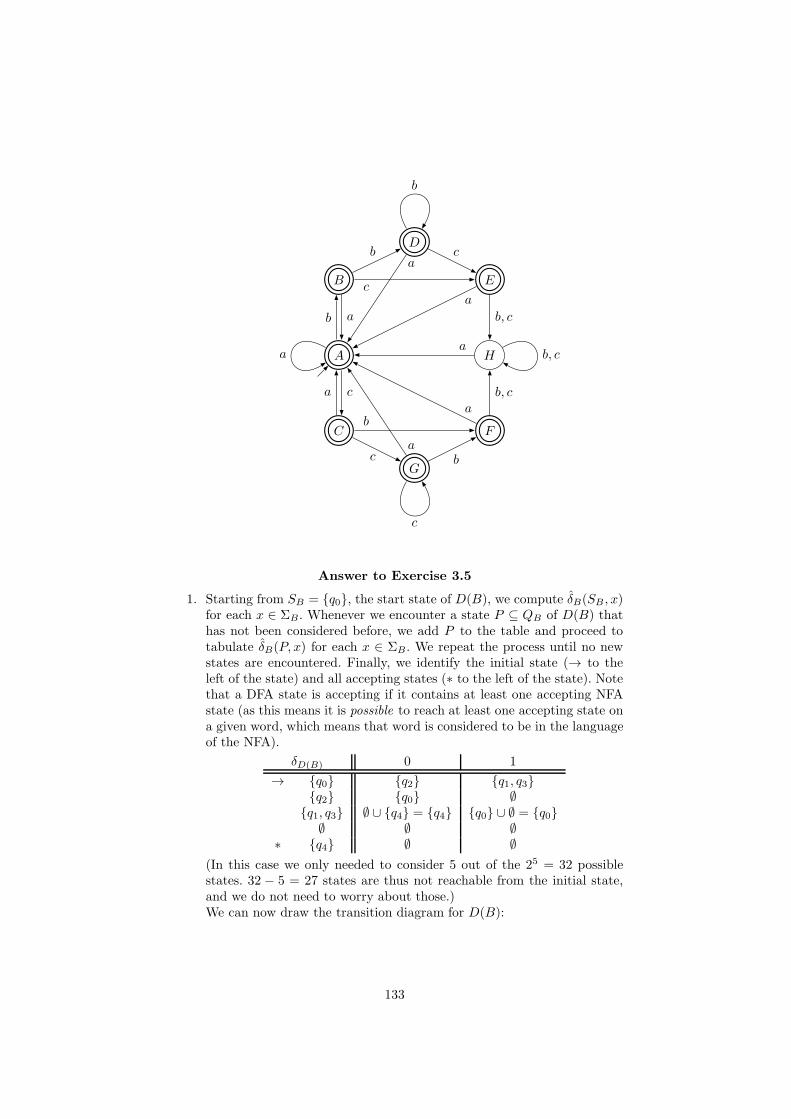
A
B
C
D
E
F
G
Ha
b a
ca
b
c
b
c
a
b
c
a
b, c
ab, c
ab
c
ab, c
Answer to Exercise 3.5
1. Starting from SB = {q0}, the start state of D(B), we compute δB(SB , x)for each x ∈ ΣB. Whenever we encounter a state P ⊆ QB of D(B) thathas not been considered before, we add P to the table and proceed totabulate δB(P, x) for each x ∈ ΣB. We repeat the process until no newstates are encountered. Finally, we identify the initial state (→ to theleft of the state) and all accepting states (∗ to the left of the state). Notethat a DFA state is accepting if it contains at least one accepting NFAstate (as this means it is possible to reach at least one accepting state ona given word, which means that word is considered to be in the languageof the NFA).
δD(B) 0 1
→ {q0} {q2} {q1, q3}{q2} {q0} ∅
{q1, q3} ∅ ∪ {q4} = {q4} {q0} ∪ ∅ = {q0}∅ ∅ ∅
∗ {q4} ∅ ∅
(In this case we only needed to consider 5 out of the 25 = 32 possiblestates. 32 − 5 = 27 states are thus not reachable from the initial state,and we do not need to worry about those.)We can now draw the transition diagram for D(B):
133
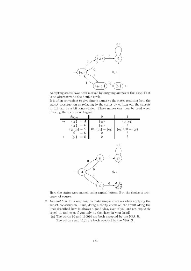
{q0}
{q2}
{q1, q3}
∅
{q4}
0
0
1
1
1
0, 1
0
0, 1
Accepting states have been marked by outgoing arrows in this case. Thatis an alternative to the double circle.It is often convenient to give simple names to the states resulting from thesubset construction as referring to the states by writing out the subsetsin full can be a bit long-winded. These names can then be used whendrawing the transition diagram:
δD(A) 0 1
→ {q0} = A {q2} {q1, q3}{q2} = B {q0} ∅
{q1, q3} = C ∅ ∪ {q4} = {q4} {q0} ∪ ∅ = {q0}∅ = D ∅ ∅
∗ {q4} = E ∅ ∅
A
B
C
D
E
0
0
1
1
1
0, 1
0
0, 1
Here the states were named using capital letters. But the choice is arbi-trary, of course.
2. General hint: It is very easy to make simple mistakes when applying thesubset construction. Thus, doing a sanity check on the result along thelines described here is always a good idea, even if you are not explicitlyasked to, and even if you only do the check in your head!(a) The words 10 and 110010 are both accepted by the NFA B.
The words ǫ and 1101 are both rejected by the NFA B.
134

(b)
word state sequence last state10 A, C, E accepting110010 A, C, A, B, A, C, E acceptingǫ A not accepting1101 A, C, A, B, D not accepting
Thus the DFA D(B) behaves like the NFA B at least for these fourwords, which should give us some reassurance as to the correctnessof the answer.
Answer to Exercise 4.1
Note: these are not necessarily the only possibilities, nor necessarily the“simplest”. But they are all fairly simple, and your answers should not be muchmore complicated.
1. (b+ c)∗a(b+ c)∗
2. (a+ c)∗b(a+ c)∗b(a+ b+ c)∗
3. (a+ b)∗(ǫ+ c)(a+ b)∗(ǫ+ c)(a + b)∗
4. (a+ b)∗(a+ c)∗
5. a∗(ba∗c+ ca∗b)a∗
6. (a(b+ c) + b+ c)∗(a+ ǫ)
7. c∗(a+ b)((a + b)c∗(a+ b) + c)∗
Answer to Exercise 4.2
L((aa+ ǫb∗∅)(b+ c))= {L(EF ) = L(E)L(F )}
L(aa+ ǫb∗∅)L(b+ c)= {L(E + F ) = L(E) ∪ L(F )} (twice)
(L(aa) ∪ L(ǫb∗∅))(L(b) ∪ L(c))= {L(EF ) = L(E)L(F )} (three times)
(L(a)L(a) ∪ L(ǫ)L(b∗)L(∅))(L(b) ∪ L(c))= {L(E∗) = (L(E))∗}
(L(a)L(a) ∪ L(ǫ)L(b)∗L(∅))(L(b) ∪ L(c))= {L(x) = {x}, L(∅) = ∅, L(ǫ) = {ǫ}}
({a}{a} ∪ {ǫ}{b}∗∅)({b} ∪ {c})= {L∅ = ∅ (twice)}
({a}{a} ∪ ∅)({b} ∪ {c})= {Set union}
{a}{a}{b, c}= {Concatenation of languages}
{aab, aac}
Answer to Exercise 4.3
States are named as they are introduced to make it easier to follow theconstruction, but it is OK to leave states unnamed to the end.
First construct an NFA for the subexpression ∅:
135

0
Then construct an NFA for the Kleene closure ∅∗. As there are no acceptingstates and thus no states immediately preceding any accepting state, there areno “loop edges” to add. But we do have to add an initial and accepting stateto account for the fact that the automaton must accept the empty word, ǫ:
0
1
It is now clear that state 0 is a dead end, so we can eliminate it already nowgiving us the NFA
1
for the subexpression ∅∗. (This is exactly what we should expect as the expres-sion is equivalent to ǫ.)
We can now consider the subexpression (a(∅∗+b))∗. In addition to the NFAfor ∅∗ constructed above, we first need NFAs for the atomic regular expressionsa (to the left) and b. We form an NFA for ∅∗ + b by placing the NFAs for ∅∗
and b in parallel (to the right):
2 3a
1
4 5b
Join the above two NFAs to obtain an NFA for a(∅∗ + b), keeping in mindthat the left DFA does not accept ǫ (“sub-case 1” in the lecture notes):
2 3a
1
4 5b
a
a
136

It is now clear state 3 is a dead end, so it can be removed prior to carryingout the construction for the Kleene closure (not forgetting one extra state foraccepting ǫ) leaving us with the following NFA A for (a(∅∗ + b))∗:
2
1
4 5
6
a
a
a
b
b
The NFA B for (c+ ǫ + ∅) is simply:
7 8
9
10
c
It’s clear that state 10 will become a dead end, so it can be removed.
Now, joining A with B (less state 10), while keeping in mind that A canaccept ǫ which means states 7 and 9 will remain initial states, gives:
2
1
4 5
6
a
a
a
b
b
7 8
9
ca
a
b
b
It’s now clear that states 1, 5, and 6 are all dead ends, so we can simplifyby removing them and obtain the final NFA for (a(∅∗ + b))∗(c+ ǫ+ ∅):
137

2
4
7 8
9
aa
a
a
b
b
b
c
Note that there are three initial states: 2, 7, and 9. Finally, it is worth spendingsome time to ensure the final NFA makes sense by comparing the words itaccepts with the words generated by the original regular expression.
Answer to Exercise 6.1
1. Straightforward, only the key steps are given. See below for an exampleof a complete proof. If n is the constant of the pumping lemma, considera specific word anbmcn+m, where m ≥ 0. This word clearly belongs to L1,and it is sufficiently long to satisfy the requirements of the lemma. Oncesplit into three parts according to the lemma, the middle part is goingto be non-empty and it is going to consist of a’s only. If the middle partis repeated, the resulting string is not going to have the right balance ofa’s, b’s, and c’s, and thus it is not going to belong to L1.
2. Assume that L2 is a regular language. Then, according to the pumpinglemma for regular languages, there exists a constant n such that anyword w ∈ L2 that has length at least n (|w| ≥ n) can be split into threeparts, w = xyz, as follows:
1. y 6= ǫ
2. |xy| ≤ n
3. ∀k ∈ N . xykz ∈ L2
Consider the word11w = a4nb2ncn. Clearly w ∈ L2. Moreover |w| = 7n ≥n. The prerequisites of the lemma are thus fulfilled, and we know it ispossible to split w into three parts x, y, and z satisfying the conditions ofthe lemma. Because our chosen word w starts with 4n a’s, and becausethe combined length of the two first parts, x and y, is at most n, weknow that x and y consists solely of a’s. Thus x = ai and y = aj forsome i, j ∈ N such that i + j ≤ n. Furthermore, because y is not emptyaccording to the lemma, we know that j > 0. z is whatever remains ofw; i.e., z = a(4n−i−j)b2ncn.
11 Note how w is chosen: it is one specific word that obviously is a word in L2, but thatdepends on the constant n in such a way that the length of w is at least n whatever n is. Itis completely wrong to assume that n is some particular value! All we know is that n exists.Also, note that the structure of w was chosen to facilitate the proof. For example, a word(aaaabbc)n is also a word in L2 with length at least n. But in this case, it is not going to bepossible to show that all ways to divide the word into three parts that satisfy the constraintsof the lemma are going to lead to a contradiction. By first establishing that n must be atleast 7 (which can be done), we will see that a division of v into x = ǫ, y = aaaabbc, andz = (aaaabbc)n−1 always is a possibility, which in turn means that all words of the form xykz
do belong to L, and we do not get any contradiction.
138

Now consider words of the form xykz. According to the pumping lemma,these words belong to L2 for any value of k. Let us consider a specificvalue for k, for example k = 0. The word xy0z should belong to L. Butxy0z = xz = aia(4n−i−j)b2ncn = a(4n−j)b2ncn. Because j > 0, it is nowclear that there are fewer than twice as many a’s as b’s in this word,which thus cannot belong to L2. We have reached a contradiction, andour assumption that L2 is a regular language must be wrong. Thus L2 isnot a regular language, QED.
Answer to Exercise 7.1
1. (a)S ⇒
GX by S → X
⇒G
ǫ by X → ǫ
orS ⇒
GY by S → Y
⇒G
ǫ by Y → ǫ
When giving derivation sequences in a context-free grammar, it isnormally not necessary to justify every single step as it is fairly obvi-ous which production is being used. The justified derivation sequenceabove were just given for explanatory purposes. Thus, an answer likethe following is perfectly OK too:
S ⇒G
X ⇒G
ǫ
or evenS ⇒ X ⇒ ǫ
as it is clear which grammar we are referring to from the context.However, to make it very clear how derivations work, we will giveexplicit justifications here.
(b)S ⇒
GX by S → X
⇒G
aXb by X → aXb
⇒G
aaXbb by X → aXb
⇒G
aabb by X → ǫ
(c)S ⇒
GY by S → Y
⇒G
cY d by Y → cY d
⇒G
ccY dd by Y → cY d
⇒G
cccY ddd by Y → cY d
⇒G
cccddd by Y → ǫ
2. No, aaaddd /∈ L(G). From the start symbol S, we can either derive X orY . However, from X it is only possible to derive strings anbn, while fromY it is only possible to derive strings cndn, neither of which are wordsstarting with a’s and ending with d’s.
139
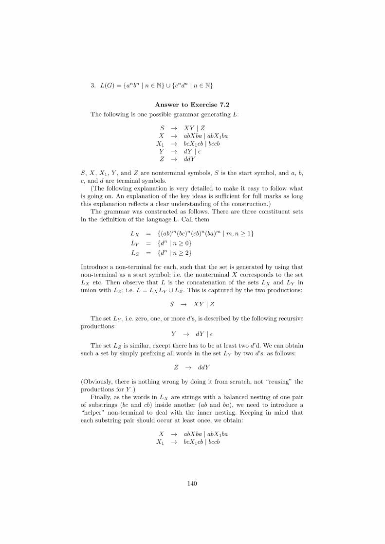
3. L(G) = {anbn | n ∈ N} ∪ {cndn | n ∈ N}
Answer to Exercise 7.2
The following is one possible grammar generating L:
S → XY | ZX → abXba | abX1baX1 → bcX1cb | bccbY → dY | ǫZ → ddY
S, X , X1, Y , and Z are nonterminal symbols, S is the start symbol, and a, b,c, and d are terminal symbols.
(The following explanation is very detailed to make it easy to follow whatis going on. An explanation of the key ideas is sufficient for full marks as longthis explanation reflects a clear understanding of the construction.)
The grammar was constructed as follows. There are three constituent setsin the definition of the language L. Call them
LX = {(ab)m(bc)n(cb)n(ba)m | m,n ≥ 1}
LY = {dn | n ≥ 0}
LZ = {dn | n ≥ 2}
Introduce a non-terminal for each, such that the set is generated by using thatnon-terminal as a start symbol; i.e. the nonterminal X corresponds to the setLX etc. Then observe that L is the concatenation of the sets LX and LY inunion with LZ ; i.e. L = LXLY ∪ LZ . This is captured by the two productions:
S → XY | Z
The set LY , i.e. zero, one, or more d’s, is described by the following recursiveproductions:
Y → dY | ǫ
The set LZ is similar, except there has to be at least two d’d. We can obtainsuch a set by simply prefixing all words in the set LY by two d’s. as follows:
Z → ddY
(Obviously, there is nothing wrong by doing it from scratch, not “reusing” theproductions for Y .)
Finally, as the words in LX are strings with a balanced nesting of one pairof substrings (bc and cb) inside another (ab and ba), we need to introduce a“helper” non-terminal to deal with the inner nesting. Keeping in mind thateach substring pair should occur at least once, we obtain:
X → abXba | abX1baX1 → bcX1cb | bccb
140
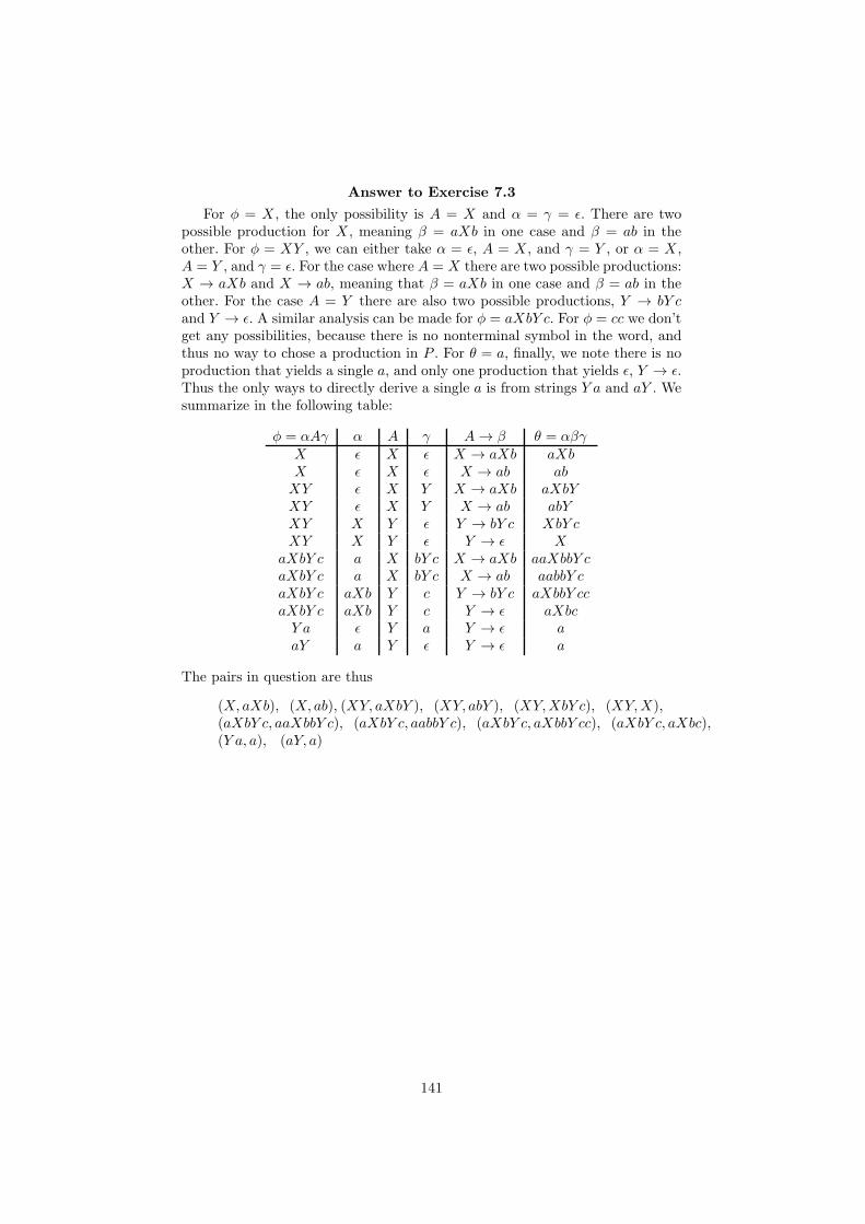
Answer to Exercise 7.3
For φ = X , the only possibility is A = X and α = γ = ǫ. There are twopossible production for X , meaning β = aXb in one case and β = ab in theother. For φ = XY , we can either take α = ǫ, A = X , and γ = Y , or α = X ,A = Y , and γ = ǫ. For the case where A = X there are two possible productions:X → aXb and X → ab, meaning that β = aXb in one case and β = ab in theother. For the case A = Y there are also two possible productions, Y → bY cand Y → ǫ. A similar analysis can be made for φ = aXbY c. For φ = cc we don’tget any possibilities, because there is no nonterminal symbol in the word, andthus no way to chose a production in P . For θ = a, finally, we note there is noproduction that yields a single a, and only one production that yields ǫ, Y → ǫ.Thus the only ways to directly derive a single a is from strings Y a and aY . Wesummarize in the following table:
φ = αAγ α A γ A → β θ = αβγX ǫ X ǫ X → aXb aXbX ǫ X ǫ X → ab abXY ǫ X Y X → aXb aXbYXY ǫ X Y X → ab abYXY X Y ǫ Y → bY c XbY cXY X Y ǫ Y → ǫ X
aXbY c a X bY c X → aXb aaXbbY caXbY c a X bY c X → ab aabbY caXbY c aXb Y c Y → bY c aXbbY ccaXbY c aXb Y c Y → ǫ aXbcY a ǫ Y a Y → ǫ aaY a Y ǫ Y → ǫ a
The pairs in question are thus
(X, aXb), (X, ab), (XY, aXbY ), (XY, abY ), (XY,XbY c), (XY,X),(aXbY c, aaXbbY c), (aXbY c, aabbY c), (aXbY c, aXbbY cc), (aXbY c, aXbc),(Y a, a), (aY, a)
141

Answer to Exercise 7.4
1. (a) Left-most derivation:
T ⇒ F ⇒ P ⇒ (T ) ⇒ (F ) ⇒ (P ) ⇒ (I) ⇒ (DI) ⇒ (7I) ⇒ (7DI)
⇒ (78I) ⇒ (78D) ⇒ (789)
Sometimes left-most derivation steps are explicitly indicated by anlm subscript as follows:
T ⇒lm
F ⇒lm
P ⇒lm
(T ) ⇒lm
. . . ⇒lm
(789)
Note that if the goal is just to derive a word, any derivation willdo, not just a left-most one (unless you’ve been explicitly asked toprovide a left-most derivation as here, of course). However, beingsystematic and sticking to e.g. left-most derivations where possiblecan help in avoiding mistakes. Anyway, to illustrate that there areother possibilities, here is a right-most derivation of the same word:
T ⇒rm
F ⇒rm
P ⇒rm
(T ) ⇒rm
(F ) ⇒rm
(P ) ⇒rm
(I) ⇒rm
(DI)
⇒rm
(DDI) ⇒rm
(DDD) ⇒rm
(DD9) ⇒rm
(D89) ⇒rm
(789)
(b) Left-most derivation:
T ⇒ T + T ⇒ F + T ⇒ P + T ⇒ I + T
⇒ D + T ⇒ 7 + T ⇒ 7 + F ⇒ 7 + F ∗ F
⇒ 7 + P ∗ F ⇒ 7 +N(A) ∗ F ⇒ 7 + g(A) ∗ F ⇒ 7 + g(T ) ∗ F
⇒ 7 + g(F ) ∗ F ⇒ 7 + g(F ∗ F ) ∗ F ⇒ 7 + g(P ∗ F ) ∗ F
⇒ 7 + g(I ∗ F ) ∗ F ⇒ 7 + g(D ∗ F ) ∗ F ⇒ 7 + g(3 ∗ F ) ∗ F
⇒ 7 + g(3 ∗ P ) ∗ F ⇒ 7 + g(3 ∗ I) ∗ F ⇒ 7 + g(3 ∗D) ∗ F
⇒ 7 + g(3 ∗ 5) ∗ F ⇒ 7 + g(3 ∗ 5) ∗ P
⇒ 7 + g(3 ∗ 5) ∗ (T ) ⇒ 7 + g(3 ∗ 5) ∗ (F ) ⇒ 7 + g(3 ∗ 5) ∗ (P )
⇒ 7 + g(3 ∗ 5) ∗ (N(A)) ⇒ 7 + g(3 ∗ 5) ∗ (f(A)) ⇒ 7 + g(3 ∗ 5) ∗ (f())
(c) It is not possible to derive 1+2 ∗ 3). There are only two productionsthat introduce parentheses, and they always introduce them as bal-anced pairs. Thus it is not possible to derive a string with a singleunmatched parenthesis as in this case.
(d) It is not possible to derive 1 + 7(9) because a number cannot befollowed directly by a left (opening) parenthesis. The substring 7(9)must have been derived from T . There are only two productions thatintroduce parentheses. The production P → N(A) cannot have beenused to derive 7(9) because, although P can be derived from T , 7cannot be derived from N . The other possibility is the productionP → (T ). But, as numbers are only derivable via I, this would onlybe possible if a word IP can be derived form T . This in turn isnot possible as the I ultimately has to be derived from a T , andinspection then shows that the only terminals that can follow an Iare +, ∗, and ).
142

2. Derivation tree:T
T
F
P
I
D
9
+T
T
F
P
)T
F
F
P
)A
T
F
P
I
D
1
(N
h
∗F
P
I
D
8
(
+T
F
P
I
D
7
3. Another derivation tree:T
T
T
F
P
I
D
9
+T
F
P
)T
F
F
P
)A
T
F
P
I
D
1
(N
h
∗F
P
I
D
8
(
+T
F
P
I
D
7
The fact that there are two different derivation trees for one word impliesthat the grammar is ambiguous.
143

4. Delete all old productions for A and add the following productions:
A → TL | ǫL → , TL | ǫ
Here, L is a new nonterminal symbol, and “,” is a new terminal symbol.The productions for L generate argument lists of zero, one or more ar-guments (any expression derivable from T ), each preceded by a comma.The production A → TL thus generates argument lists of one or morearguments separated by commas, while the production A → ǫ takes careof the case of zero arguments.
Answer to Exercise 8.1
The problem is that the grammar does not impart any associativity on theoperators + and ∗. Let us make them left-associative to address this. (Mak-ing them right-associative would also work, but we cannot make them non-associative as that would change the language; e.g. the example word 7 + (8 ∗h(1)) + 9 would no longer belong to the language as non-associativity meanswe have to use explicit bracketing.) We make those operators left-associative bymaking the corresponding productions left-recursive:
T → T + F | FF → F ∗ P | P
Answer to Exercise 8.2
First identify the nonterminals for which there are immediately left-recursiveproductions. Then group the productions for each such non-terminal into twogroups: one where each RHS starts with the nonterminal in question (the im-mediately left-recursive terminals), and one where they don’t:
A → Aα1 | . . . | Aαm
A → β1 | . . . | βn
In our case, there are immediately left-recursive productions for S and X inthe given grammar. Grouping the productions as required yields:
• Grouping of productions for S:
S → Sa
S → XbS | a
• Grouping of productions for X :
X → XXX | XY Y
X → Y Y Y | Y Y X
144

• Remaining productions:
Y → cY | dY | e
Then, continuing with the general example, the productions for a nonter-minal A for which there are immediately left-recursive productions need to bereplaced with new productions for A and productions for A′, where A′ is a newname, as follows:
A → β1A′ | . . . | βnA
′
A′ → α1A′ | . . . | αmA′|ǫ
In our case, this transformation needs to be applied to the productions forthe nonterminals S and X
S → XbSS′ | aS′
S′ → aS′ | ǫ
X → Y Y Y X ′ | Y Y XX ′
X ′ → XXX ′ | Y Y X ′ | ǫ
Y → cY | dY | e
Note in particular how the production X → XXX was transformed. Thetransformation rule specifies that the right-hand side should be split after thefirst X , meaning that the “α-part” is XX in this case. It might be confusingthat this still starts with an X , but that is what the transformation rule says,and it is fairly easy to see why with a bit of thought. Then the XX is used toconstruct one of the right-recursive productions for the new nonterminal X ′.
Answer to Exercise 10.1
1. Nǫ = {S,A,B}. A is nullable because A → ǫ is a production. B isnullable because B → ǫ is a production. S is nullable because S → ABBis a production and both A and B are nullable. C is not nullable becausethe RHSs of all productions for C include a terminal (c or d), meaningit is clear ǫ cannot be derived from C.
2. Keeping in mind which non-terminals are nullable, we obtain the follow-ing equations:
first(A) = first(aA) ∪ first(ǫ)
= {a} ∪ ∅
= {a}
first(B) = first(Bb) ∪ first(ǫ)
= (first(B) ∪ first(b)) ∪ ∅
= first(B) ∪ first(b)
first(C) = first(cA) ∪ first(d)
= first(c) ∪ first(d)
= {c} ∪ {d}
= {c, d}
145

The solutions of the equations for first(A) and first(C) are manifest. Asto the equation for first(B), we need only observe that it has the formX = X ∪ Y and that there are no further constraints on first(B). Thesmallest solution to such an equation is simply X = Y , so first(B) = {b}.Now we can turn to setting up and solving the equation for first(S), againkeeping in mind which non-termainals are nullable:
first(S) = first(ABB) ∪ first(BBC) ∪ first(CA)
= (first(A) ∪ first(B) ∪ first(B) ∪ first(ǫ))
∪ (first(B) ∪ first(B) ∪ first(C))
∪first(C)
= (first(A) ∪ first(B) ∪ ∅)
∪ (first(B) ∪ first(C))
∪first(C)
= ({a} ∪ {b}) ∪ ({b} ∪ {c, d}) ∪ ({c, d})
= {a, b, c, d}
Thus, we obtained a solution directly.
3. Note: very detailed account below for clarity. It is sufficient to just statethe constraints according to the definitions and then simplify.Constraints for follow(S):
{$} ⊆ follow(S)
Constraints for follow(A) from the productions where A occurs in theRHS, i.e.
S → ABB
S → CA
A → aA
(note: nullable(BB) and nullable(ǫ)):
first(BB) ⊆ follow(A)
follow(S) ⊆ follow(A)
first(ǫ) ⊆ follow(A)
follow(S) ⊆ follow(A)
first(ǫ) ⊆ follow(A)
follow(A) ⊆ follow(A)
Constraints for follow(B) from the productions where B occurs in theRHS, i.e.
S → ABB
S → BBC
B → Bb
146

(note: nullable(B) and nullable(ǫ)):
first(B) ⊆ follow(B)
follow(S) ⊆ follow(B)
first(ǫ) ⊆ follow(B)
follow(S) ⊆ follow(B)
first(BC) ⊆ follow(B)
first(C) ⊆ follow(B)
first(b) ⊆ follow(B)
Constraints for follow(C) from the productions where C occurs in theRHS, i.e.
S → BBC
S → CA
C → cC
(note: nullable(A) and nullable(ǫ)):
first(ǫ) ⊆ follow(C)
follow(S) ⊆ follow(C)
first(A) ⊆ follow(C)
follow(S) ⊆ follow(C)
first(ǫ) ⊆ follow(C)
follow(C) ⊆ follow(C)
Using
first(ǫ) = ∅
first(A) = {a}
first(B) = {b}
first(C) = {c, d}
first(BB) = first(B) ∪ first(B) ∪ first(ǫ)
= {b} ∪ {b} ∪ ∅ = {b}
first(BC) = first(B) ∪ first(C) ∪ ∅
= {b} ∪ {c, d} = {b, c, d}
and eliminating trivial constraints yields:
147
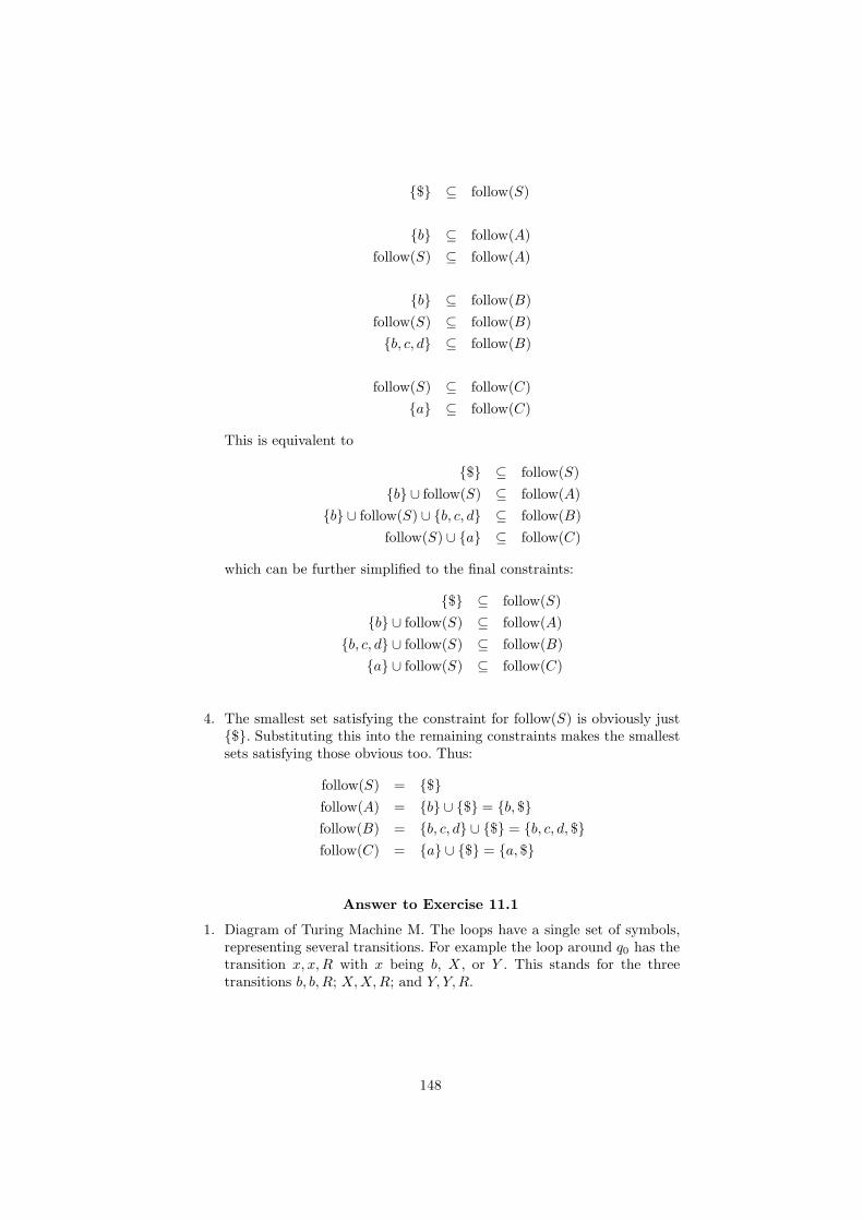
{$} ⊆ follow(S)
{b} ⊆ follow(A)
follow(S) ⊆ follow(A)
{b} ⊆ follow(B)
follow(S) ⊆ follow(B)
{b, c, d} ⊆ follow(B)
follow(S) ⊆ follow(C)
{a} ⊆ follow(C)
This is equivalent to
{$} ⊆ follow(S)
{b} ∪ follow(S) ⊆ follow(A)
{b} ∪ follow(S) ∪ {b, c, d} ⊆ follow(B)
follow(S) ∪ {a} ⊆ follow(C)
which can be further simplified to the final constraints:
{$} ⊆ follow(S)
{b} ∪ follow(S) ⊆ follow(A)
{b, c, d} ∪ follow(S) ⊆ follow(B)
{a} ∪ follow(S) ⊆ follow(C)
4. The smallest set satisfying the constraint for follow(S) is obviously just{$}. Substituting this into the remaining constraints makes the smallestsets satisfying those obvious too. Thus:
follow(S) = {$}
follow(A) = {b} ∪ {$} = {b, $}
follow(B) = {b, c, d} ∪ {$} = {b, c, d, $}
follow(C) = {a} ∪ {$} = {a, $}
Answer to Exercise 11.1
1. Diagram of Turing Machine M. The loops have a single set of symbols,representing several transitions. For example the loop around q0 has thetransition x, x,R with x being b, X , or Y . This stands for the threetransitions b, b, R; X,X,R; and Y, Y,R.
148
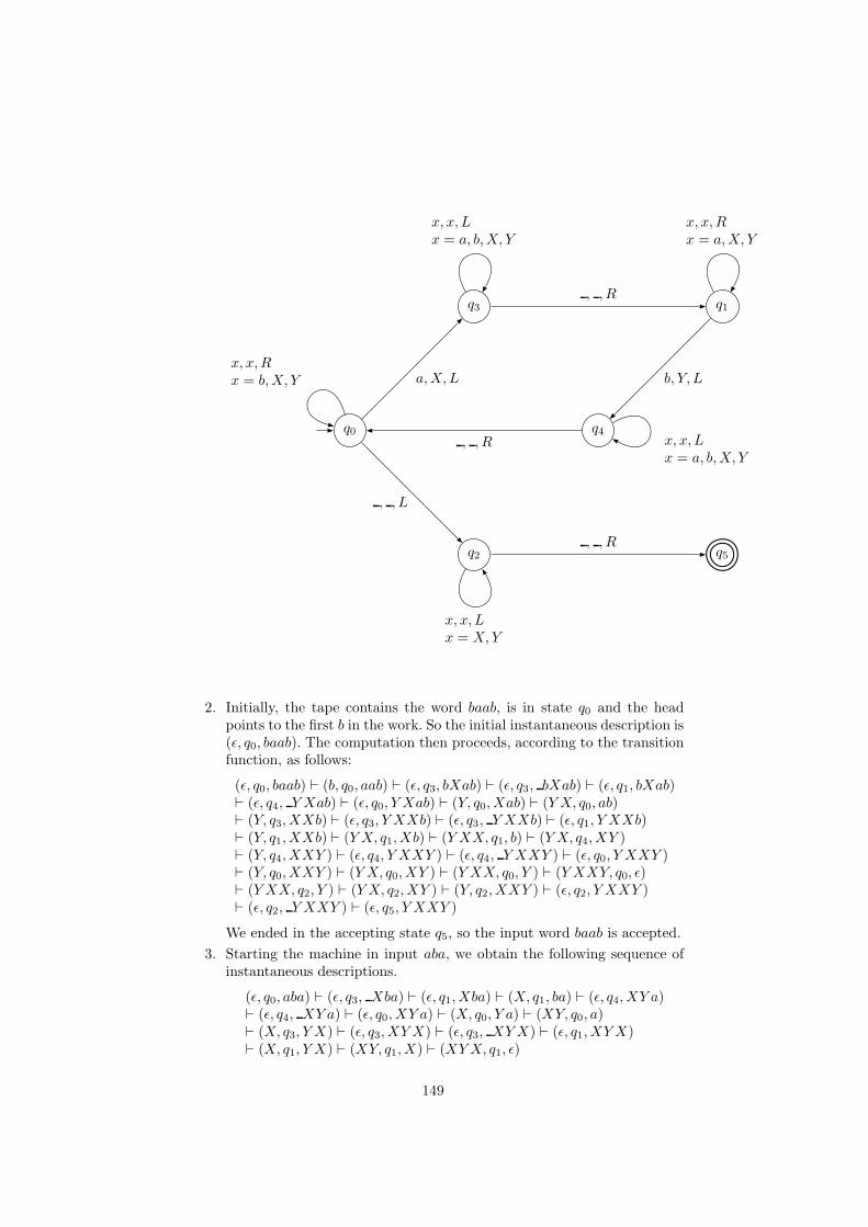
q0
q3 q1
q4
q2 q5
a,X,Lx, x,Rx = b,X, Y
, , L
b, Y, L
x, x,Rx = a,X, Y
, , R
x, x, Lx = X,Y
, , R
x, x, Lx = a, b,X, Y
, , R x, x, Lx = a, b,X, Y
2. Initially, the tape contains the word baab, is in state q0 and the headpoints to the first b in the work. So the initial instantaneous description is(ǫ, q0, baab). The computation then proceeds, according to the transitionfunction, as follows:
(ǫ, q0, baab) ⊢ (b, q0, aab) ⊢ (ǫ, q3, bXab) ⊢ (ǫ, q3, bXab) ⊢ (ǫ, q1, bXab)⊢ (ǫ, q4, Y Xab) ⊢ (ǫ, q0, Y Xab) ⊢ (Y, q0, Xab) ⊢ (Y X, q0, ab)⊢ (Y, q3, XXb) ⊢ (ǫ, q3, Y XXb) ⊢ (ǫ, q3, Y XXb) ⊢ (ǫ, q1, Y XXb)⊢ (Y, q1, XXb) ⊢ (Y X, q1, Xb) ⊢ (Y XX, q1, b) ⊢ (Y X, q4, XY )⊢ (Y, q4, XXY ) ⊢ (ǫ, q4, Y XXY ) ⊢ (ǫ, q4, Y XXY ) ⊢ (ǫ, q0, Y XXY )⊢ (Y, q0, XXY ) ⊢ (Y X, q0, XY ) ⊢ (Y XX, q0, Y ) ⊢ (Y XXY, q0, ǫ)⊢ (Y XX, q2, Y ) ⊢ (Y X, q2, XY ) ⊢ (Y, q2, XXY ) ⊢ (ǫ, q2, Y XXY )⊢ (ǫ, q2, Y XXY ) ⊢ (ǫ, q5, Y XXY )
We ended in the accepting state q5, so the input word baab is accepted.
3. Starting the machine in input aba, we obtain the following sequence ofinstantaneous descriptions.
(ǫ, q0, aba) ⊢ (ǫ, q3, Xba) ⊢ (ǫ, q1, Xba) ⊢ (X, q1, ba) ⊢ (ǫ, q4, XY a)⊢ (ǫ, q4, XY a) ⊢ (ǫ, q0, XY a) ⊢ (X, q0, Y a) ⊢ (XY, q0, a)⊢ (X, q3, Y X) ⊢ (ǫ, q3, XY X) ⊢ (ǫ, q3, XY X) ⊢ (ǫ, q1, XY X)⊢ (X, q1, Y X) ⊢ (XY, q1, X) ⊢ (XYX, q1, ǫ)
149
The machine is in state q1 and is reading a blank. There are no transitionsfor blank from q1, so the machine stops. Since q1 is not an accepting state,the input word aba is rejected.
4. This machine accepts the words in {a, b} that contain the same numberof as and bs. The language accepted by this Turing Machine is
L(M) = {w ∈ {a, b}∗ | #a(w) = #b(w)}
where I used the notation #x(w) for the number of occurrences of thesymbol x in the word w.To see this, think about what happens in each of the states. You cancharacterize each state by performing some action:
q0: Look for the next a, replace it with X and change to q3. If you don’tfind any more as, change to q2.
q3: Go back to the beginning of the word and change to q1.
q1: Look for the next b, replace it with Y and change to q4. If you don’tfind any more bs, stop and reject.
q4: Go back to the beginning of the word and change to q0 (start again).
q2: Go through the word from right to left, checking that it containsonly Xs and Y s (if it contains some a or b, stop and reject), thenmove to q5.
q5: Accept.
So the machine repeatedly searches for an a (state q0) and replaces itwith X , then searches for a b (state q1) and replaces it with Y . It pairsthem repeatedly; if it fails to pair an a with a b, it stops and reject.When it has finished all the as, it goes through the word again (state q2)checking that there are no bs left. In that case it knows that each a hasbeen paired with a b with nothing left over; only in that case it moves toq5 and accepts.
Answer to Exercise 11.2
There are several ways of implementing a Turing Machine that performs thecomputation required. The following is very simple, but does what is necessary.
1. This is the diagram illustrating the machine:
150

q0
q1
q2
a, a,Rb, b, R
b, b, R
a, b, L
b, a, L
The machine starts at the beginning of the tape, skipping over the as instate q0. As soon as it finds a b, it changes to q1 and starts skipping overthe bs. If it gets to the end of the word, it means that the symbols are inthe correct order and it stops. But if it finds an a while in q1, it knowsthat this a came after at least one b: we found a pair of symbols in thewrong order. We replace this a with a b and we replace the b that camebefore it with an a (state q2). We are now in the position before this pairand we can return to q0 and start looking for another wrong pair.
2. The machine is formally defined as follows:
M = (Q,Σ,Γ, δ, q0, , ∅) where Q = {q0, q1, q2, }Σ = {a, b}Γ = {a, b, }
(The set of accepting states is empty, because the problem does notrequire that we accept words in a certain language.)The transition function is defined by:
δ(q0, a) = (q0, a, R)δ(q0, b) = (q1, b, R)δ(q1, a) = (q2, b, L)δ(q1, b) = (q1, b, R)δ(q2, b) = (q0, a, L)
151
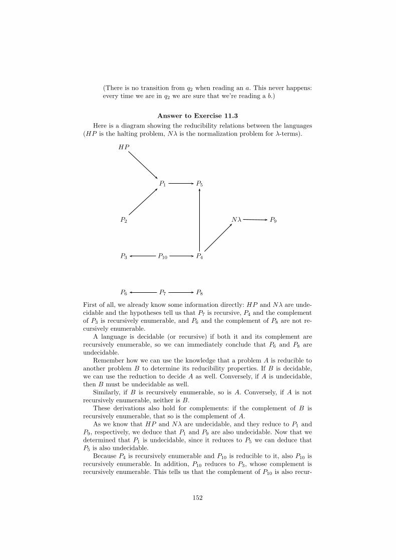
(There is no transition from q2 when reading an a. This never happens:every time we are in q2 we are sure that we’re reading a b.)
Answer to Exercise 11.3
Here is a diagram showing the reducibility relations between the languages(HP is the halting problem, Nλ is the normalization problem for λ-terms).
HP
P1 P5
P2 Nλ P9
P3 P10 P4
P6 P7 P8
First of all, we already know some information directly: HP and Nλ are unde-cidable and the hypotheses tell us that P7 is recursive, P4 and the complementof P3 is recursively enumerable, and P6 and the complement of P8 are not re-cursively enumerable.
A language is decidable (or recursive) if both it and its complement arerecursively enumerable, so we can immediately conclude that P6 and P8 areundecidable.
Remember how we can use the knowledge that a problem A is reducible toanother problem B to determine its reducibility properties. If B is decidable,we can use the reduction to decide A as well. Conversely, if A is undecidable,then B must be undecidable as well.
Similarly, if B is recursively enumerable, so is A. Conversely, if A is notrecursively enumerable, neither is B.
These derivations also hold for complements: if the complement of B isrecursively enumerable, that so is the complement of A.
As we know that HP and Nλ are undecidable, and they reduce to P1 andP9, respectively, we deduce that P1 and P9 are also undecidable. Now that wedetermined that P1 is undecidable, since it reduces to P5 we can deduce thatP5 is also undecidable.
Because P4 is recursively enumerable and P10 is reducible to it, also P10 isrecursively enumerable. In addition, P10 reduces to P3, whose complement isrecursively enumerable. This tells us that the complement of P10 is also recur-
152

sively enumerable. We derived that both P10 and its complement are recursivelyenumerable, therefore P10 is recursive.
The rest of the given information does not add anything to our knowledge.For example, knowing that P2 is reducible to the undecidable problem P1 doesn’treveal anything about P2.
1. Undecidable: P1, P5, P6, P8, P9
2. Recursively enumerable: P4, P7, P10
3. Recursive: P7, P10
Answer to Exercise 12.1
1. The function nand-pair takes a pair of Booleans p and returns a pairof Booleans whose first element is the negation of the conjunction ofthe elements of p, and whose second element is simply the first of p.(Remember that p true is the first projection of p and p false is the secondprojection.) So we have:
nand-pair 〈true, true〉 ∗ 〈false, true〉nand-pair 〈true, false〉 ∗ 〈true, true〉
nand-pair 〈false, true〉 ∗ 〈true, false〉nand-pair 〈false, false〉 ∗ 〈true, false〉
2. Remember that Church numerals are just iterators, so the definition ofnand-fun tells us to iterate n times the function nand-pair starting with theinitial value 〈false, false〉. Applied to the numeral 4 = λf.λx.f (f (f (f x)))it produces the following reduction steps:
nand-fun 4 = (λn.n nand-pair 〈false, false〉) 4 4 nand-pair 〈false, false〉 = (λf.λx.f (f (f (f x)))) nand-pair 〈false, false〉
∗ nand-pair (nand-pair (nand-pair (nand-pair 〈false, false〉)))
∗ nand-pair (nand-pair (nand-pair 〈true, false〉))
∗ nand-pair (nand-pair 〈true, true〉)
∗ nand-pair 〈false, true〉
∗ 〈true, false〉
3. As the previous calculation shows, nand-funn iterates n times nand-pair,starting with the initial value 〈false, false〉. So nand-fun 0 will do zeroiterations and just return this initial value. The sequence of values thatthe iteration goes through is obtained by repeating the steps of part (a).Here are the values obtained (with the iteration number written on topof the arrows):
〈false, false〉1
−→ 〈true, false〉2
−→ 〈true, true〉3
−→ 〈false, true〉4
−→ 〈true, false〉5
−→ 〈true, true〉6
−→ 〈false, true〉7
−→ 〈true, false〉8
−→ 〈true, true〉9
−→ · · ·
We obtain 〈true, true〉 for 2, 5 and 8. It is clear that there is a cycle thatrepeats every three steps, so we have nand-funn ∗ 〈true, true〉 for thosenumbers n of the form n = 2 + 3 ∗m for some m.
153

Answer to Exercise 12.2
To implement thrFib in the λ-calculus, we need to see it as the iteration ofa function a number of times starting with a given value. As in the case of theFibonacci function described in the lecture, we need to use an auxiliary functionthat returns three values at the same time (it was just two for Fibonacci). Thenat each step we shift two of the values and add the sum of the three:
〈n,m, k〉 7−→ 〈m, k, n+m+ k〉.
Informally, our auxiliary function is defined by
thrFibaux : N → N× N× N
thrFibaux 0 = 〈0, 0, 1〉thrFibaux (n+ 1) = 〈m, k, n+m+ k〉 where 〈n,m, k〉 = thrFibaux n
In the λ-calculus we use the encoding of triples as
〈a, b, c〉 = λx.x a b c
With the projections defined by
fst = λt.t (λx.λy.λz.x), snd = λt.t (λx.λy.λz.y), trd = λt.t (λx.λy.λz.z).
(You can also encode triples as repeated pairs. It is not important how you doit, as long as you can define projections.)
Using triples and their projections, we can define the auxiliary function inλ-calculus:
thrFibaux = λn.n step 〈0, 0, 1〉where step = λt.〈snd t, trd t, plus (fst t) (plus (snd t) (trd t))〉
Finally, the function we want will just take the first component of the result ofthe auxiliary function:
thrFib = λn.fst (thrFibaux n).
Answer to Exercise 13.1
The function evaluate can be defined by recursion on the structure of theSAT formula, using just the projection from the assignment to determine thevalue on the variables.
evaluate :: SAT -> Assignment -> Bool
evaluate (Var i) a = a!!i
evaluate (Not x) a = not (evaluate x a)
evaluate (And x y) a = (evaluate x a) && (evaluate y a)
evaluate (Or x y) a = (evaluate x a) || (evaluate y a)
Note that in the variable case, if the index i is larger or equal to the lengthof the assignment list, we would get an error. But we are assuming that weevaluate expressions with assignments that guarantee values for all variablesoccurring in the expression.
154

Answer to Exercise 13.2
1. The function varNum is also defined by recursion on the structure of theexpression, returning just the index for variables and the maximum ofthe recursive calls for conjunctions and disjunctions.
varNum :: SAT -> Int
varNum (Var n) = n
varNum (Not x) = varNum x
varNum (And x y) = max (varNum x) (varNum y)
varNum (Or x y) = max (varNum x) (varNum y)
2. Notice that the length of the assignment returned by allAssign n isn + 1 (it must contain all the possible values for variables Var 0, . . . ,Var n, that is the first n + 1 variables). So allAssign 0 should return[[True],[False]]. We may use this as a base case. For the recursivecase, we can just add either a True or a False in front of each of the listcomputed by the recursive call.
allAssign :: Int -> [Assignment]
allAssign 0 = [[True],[False]]
allAssign n = [b:bs | b <- [True,False],
bs <- allAssign (n-1)]
(An alternative solution for the base case is allAssign (-1) = [[]].)
3. Evaluate the formula using all the possible assignments for its variables.If at least one of them returns True, then the formula is satisfiable.
satisfiable :: SAT -> Bool
satisfiable x = or (map (evaluate x)
(allAssign (varNum x)))
4. From the list of all assignments, filter out those that return True. If thislist is empty, then the formula is not satisfiable. If it is not empty, anyof its elements (for example the head) is a solution.
solution :: SAT -> Maybe Assignment
solution x = if null bs then Nothing else Just (head bs)
where bs = filter (evaluate x)
(allAssign (varNum x))
Answer to Exercise 13.3
1. The program evaluate traverses the whole structure of the input for-mula. For the Not, And and Or operators it simply calls itself on thesubformulas and then does a simple operation. In the variable case itjust looks up the value in the assignment, which is linear in the length ofthe assignment.So the number of operations executed at each step is at most linear inthe length of the assignment. The number of steps is bound by the sizeof the formula. So the overall complexity is at most quadratic on the sizeof the input.
155
2. The function satisfiable applies evaluate to all the possible assign-ments of values to the variables. Each application of evaluate takes poly-nomial time, but there are exponentially many assignments that need tobe tested; to be precise, for n variables there are 2n assignments. Since weare performing the evaluation for each of these assignments, the overallcomplexity is also exponential.
3. The fact that SAT is NP-complete means that every NP problem canbe reduced to it in polynomial time. This means that if we ever find apolynomial time algorithm for SAT, we would automatically be able tosolve all NP problems in polynomial time. This would prove that NP= P .
156

References
[ASU86] Alfred V. Aho, Ravi Sethi, and Ullman Jeffrey D. Ullman. Compilers- Principles, Techniques, and Tools. Addison-Wesley, 1986. 90
[Cox07] Russ Cox. Regular expression matching can be simple andfast (but is slow in java, perl, php, python, ruby, ...).http://swtch.com/ rsc/regexp/regexp1.html, January 2007. 29
[GJS+15] James Gosling, Bill Joy, Guy Steele, Gilad Bracha, and Alex Buckley.The Java Language Specification. Oracle, Inc., Java SE 8 editionedition, 2015. 62
[HMU01] John E. Hopcroft, Rajeev Motwani, and Jeffrey D. Ullman. Intro-duction to Automata Theory, Languages, and Computation. AddisonWesley, 2nd edition edition, 2001. 17, 44, 79, 102
[Hud99] Scott E. Hudson. Cup parser generator for java.http://www.cs.princeton.edu/∼appel/modern/java/CUP/, 1999. 99
[Mar01] Simon Marlow. Happy: The parser generator for haskell.http://www.haskell.org/happy/, 2001. 99
[Nil16] Henrik Nilsson. Compilers (G53CMP) — lecture notes.http://www.cs.nott.ac.uk/∼nhn/G53CMP, 2016. 62, 82
[Par05] Terence Parr. ANTLR: Another tool for language recognition.http://www.antlr.org/, 2005. 99
157