MCS 7 Chia Laguna, Cagliari, Sardinia, Italy, September 11-15, 2011

LARGE EDDY SIMULATION OF A GAS TURBINE COMBUSTIONCHAMBER

G. Bulat∗, W. P. Jones∗∗, A. Marquis∗∗, V. Sanderson∗ and U. Stopper∗∗∗w.jones@imperial.ac.uk

∗ Siemens Industrial Turbomachinery Ltd, Waterside South, Lincoln LN5 7FD, UK∗∗ Imperial College London, Exhibition Road, London SW7 2AZ, UK

∗∗∗ German Aerospace Centre (DLR), Pfaffenwaldring, Stuttgart D-70569, Germany

AbstractAn industrial gas turbine burner operating at a pressure of 3 bar is simulated using the

sgs-pdf evolution equation approach in conjunction with the Eulerian stochastic field solutionmethod in the context of Large Eddy Simulation. A dynamic version of the Smagorinsky modelis adopted for the sub-grid stresses and eight stochastic fields were utilised to characterize theinfluence of the sub-grid fluctuations. The chemistry was represented by an ARM reducedGRI 3.0 mechanism with 15 reaction steps and 19 species. The results show good agreementwith the experimental data in the flame region at different axial locations. The results serveto demonstrate that simulations of complex combustion problems in industrial geometries areachievable.

IntroductionThe turbulent premixed flames to be found in industrial gas turbine combustors are difficult

to study due to high levels turbulence, fast chemistry and complex geometrical features. Mostof these devices operate at high pressure, which adds to the difficulty of obtaining experimen-tal data and accounting for pressure effects in computational models. Large Eddy Simulation(LES) is a powerful and promising modelling technique particularly for highly swirling and un-steady flows. In case of LES of turbulent combustion, account must be taken of the interactionsbetween turbulence and chemical reaction. The main difficulties encountered in achieving thisarise from the filtered chemical source terms, which represents the net rate of species formationand consumption through chemical reaction. Since these reactions are highly non-linear, thefiltered values of the fields of chemical species mass fraction and temperature are strongly in-fluenced by the sub-grid scale (sgs) fluctuations of the reactants and the temperature. A methodof accounting for these is from the joint scalar probability density function (pdf ) of all the rel-evant scalar quantities which provides all the necessary information required to evaluate thefiltered chemical source terms.

The modelled form of the equation governing the time evolution of the joint pdf of thecomplete set of scalars provides a means of determining all of the time and spatially varyingone-point statistics. The chemical source terms appear in closed form in this equation and nofurther modelling is required, beyond specification of a chemical reaction mechanism. Dueto the high dimensionality of the pdf evolution equation, a solution only becomes feasible ifstochastic methods are applied. Conventionally Lagrangian stochastic particle methods havebeen adopted for the pdf equation in conjunction with an Eulerian formulation for the velocityand pressure fields. Alternatively, Eulerian approaches have been formulated (see [1] and [2]).These methods introduce stochastic fields, which form a system of stochastic partial differentialequations having the same one-point moments as the modelled pdf evolution equation, e.g. [3].A main advantage of the latter method is that the solutions give rise to fields that are continuous

and differentiable in space and which are thus free of spatially varying stochastic errors.

Main ObjectivesThe LES-pdf formulation in conjunction with the Eulerian stochastic field solution method

has been successfully applied in a range of burning configurations: ignition [4, 5] and auto-ignition [6], [7], non-premixed [8] and premixed regimes [9]. The majority of cases were atatmospheric pressure and in relatively simple geometrical configurations. This paper aims tovalidate the LES-pdf method for an industrial gas turbine burner (Siemens SGT-100), 1 MWthermal power operating at a pressure of 3 bar. Although the geometrical features of the burnerwere retained, the operating conditions (pressure, temperature and mixture fractions) studiedand discussed in this paper differ from those of the burner in SGT-100 gas turbine. The burner,

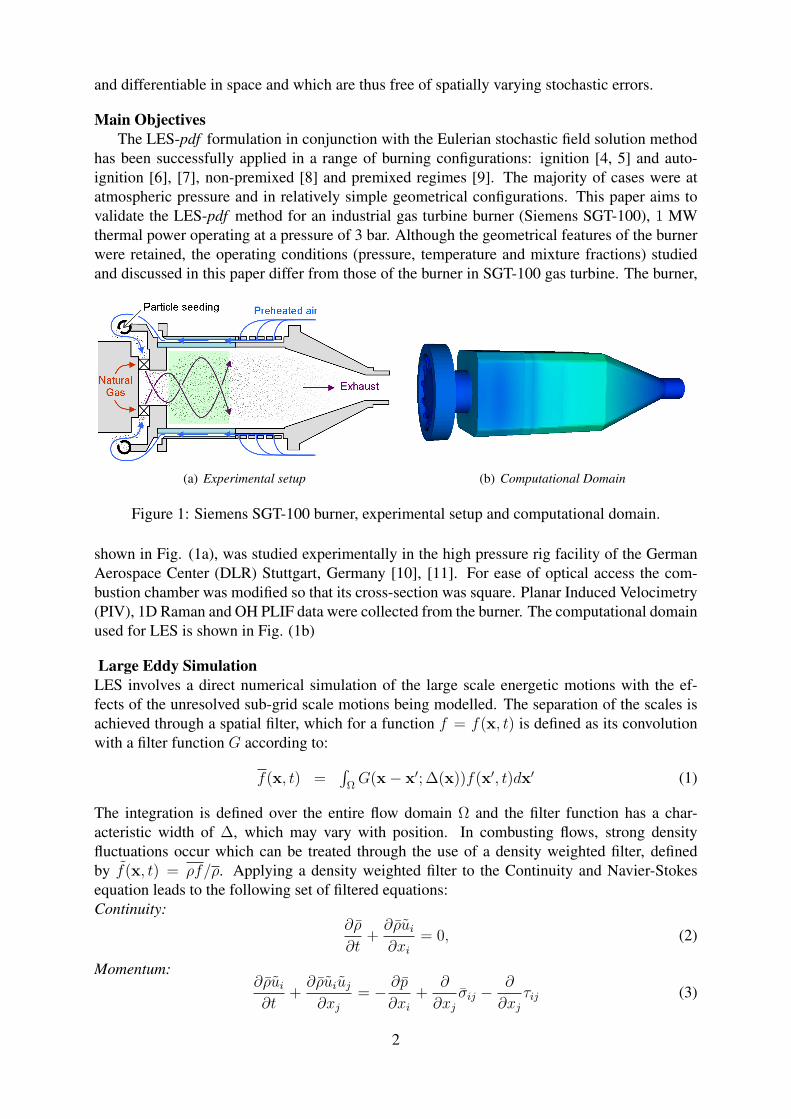
(a) Experimental setup (b) Computational Domain

Figure 1: Siemens SGT-100 burner, experimental setup and computational domain.

shown in Fig. (1a), was studied experimentally in the high pressure rig facility of the GermanAerospace Center (DLR) Stuttgart, Germany [10], [11]. For ease of optical access the com-bustion chamber was modified so that its cross-section was square. Planar Induced Velocimetry(PIV), 1D Raman and OH PLIF data were collected from the burner. The computational domainused for LES is shown in Fig. (1b)

Large Eddy SimulationLES involves a direct numerical simulation of the large scale energetic motions with the ef-fects of the unresolved sub-grid scale motions being modelled. The separation of the scales isachieved through a spatial filter, which for a function f = f(x, t) is defined as its convolutionwith a filter function G according to:

f(x, t) =∫ΩG(x− x′; ∆(x))f(x′, t)dx′ (1)

The integration is defined over the entire flow domain Ω and the filter function has a char-acteristic width of ∆, which may vary with position. In combusting flows, strong densityfluctuations occur which can be treated through the use of a density weighted filter, definedby f(x, t) = ρf/ρ. Applying a density weighted filter to the Continuity and Navier-Stokesequation leads to the following set of filtered equations:Continuity:

∂ρ

∂t+∂ρui∂xi

= 0, (2)

Momentum:∂ρui∂t

+∂ρuiuj∂xj

= − ∂p

∂xi+

∂

∂xjσij −

∂

∂xjτij (3)

2

where σij is the viscous stress tensor and D is the diffusivity, assumed equal for all speciesand enthalpy. The sub-grid scale stress tensor τij = ρ (uiuj − uiuj) is determined via thedynamically calibrated version of the Smagorinsky model proposed by Piomelli and Liu [12].The filter width ∆ is taken as the cubic root of the local grid cell volume.

The filtered forms of the conservation equations for specific molar mass of the chemicalspecies contain the filtered net formation rates of the chemical species through chemical re-action. The direct evaluation of these poses serious difficulties and to overcome these a jointsgs-pdf evolution equation formulation is adopted.

Sub-grid joint pdfAn exact equation describing the evolution of the joint sub-grid (or more strictly the filtered

fine grained) pdf Psgs can be derived by standard methods, e.g. [13]. This equation containsunknown terms, representing sgs-transport of pdf and sgs micro-mixing. In the present workthese are represented, respectively, by a Smagorinsky type gradient model and by the LinearMean Square Estimation (LMSE) closure, [14]. With these models incorporated the joint —pdfequation for the N scalar quantities needed to describe reaction can be written:

ρ∂Psgs(ψ)

∂t+ ρuj

∂Psgs(ψ)

∂xj−

N∑α=1

∂

∂ψα

[ρωα(ψ)Psgs(ψ)

]=

+∂

∂xi

[((µ

σ+µsgs

σsgs

)∂Psgs(ψ)

∂xi

)]− ρ

τsgs

N∑α=1

∂

∂ψα

[(ψα − ϕα(x, t))Psgs(ψ)

] (4)

where σsgs is assigned the value 0.7 where ωα(ψ) is, in the case of chemical species the netformation rate through chemical reaction. The number of scalar quantities, N is equal to thenumber of chemical species considered plus one (enthalpy). The micro-mixing time scale isobtained from τsgs

−1 = Cdµ+µsgs

ρ∆2 , where Cd = 2.

Eulerian stochastic field methodThe equation describing the evolution of the pdf, equation 4 is solved using the Eulerian

stochastic field method. Psgs(ψ) is represented by an ensemble of Ns stochastic fields for eachof the N scalars, namely ξnα(x, t) for 1 ≤ n ≤ Ns, 1 ≤ α ≤ N . In the present work the Itoformulation of the stochastic integral is adopted and the stochastic fields thus evolve accordingto:

dξnα = −ui∂ξnα∂xi

dt+∂

∂xi

[Γ′∂ξ

nα

∂xi

]dt+ (2Γ′)

1/2 ∂ξnα

∂xidW n

i − 1

2τsgs

(ξnα − ϕα

)dt+ ωn

α(ξn)dt ,

(5)

where Γ′ represents the total diffusion coefficient and dW ni represent increments of a (vector)

Wiener process, different for each field but independent of the spatial location x. This stochasticterm has no influence on the first moments (or mean values) of ξnα. The stochastic fields givenby (5) are not to be mistaken with any particular realization of the real field, but rather form anequivalent stochastic system (both sets have the same one-point pdf, [3]) smooth over the scaleof the filter width.

Computational DetailsThe SGT-100 Dry Low Emission (DLE) burner operating at 3 bar pressure conditions was

selected as a test case. The Siemens DLE technology has been proven in the field over the past22 years and more than 20 million hours of operational experience has been accumulated. The

3

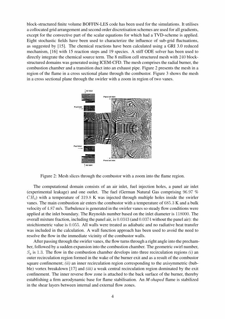
block-structured finite volume BOFFIN-LES code has been used for the simulations. It utilisesa collocated grid arrangement and second order discretisation schemes are used for all gradients,except for the convective part of the scalar equations for which had a TVD-scheme is applied.Eight stochastic fields have been used to characterize the influence of sub-grid fluctuations,as suggested by [15]. The chemical reactions have been calculated using a GRI 3.0 reducedmechanism, [16] with 15 reaction steps and 19 species. A stiff ODE solver has been used todirectly integrate the chemical source term. The 8 million cell structured mesh with 240 block-structured domains was generated using ICEM-CFD. The mesh comprises the radial burner, thecombustion chamber and a transition duct into an exhaust pipe. Figure 2 presents the mesh in aregion of the flame in a cross sectional plane through the combustor. Figure 3 shows the meshin a cross sectional plane through the swirler with a zoom in region of two vanes.

Figure 2: Mesh slices through the combustor with a zoom into the flame region.

The computational domain consists of an air inlet, fuel injection holes, a panel air inlet(experimental leakage) and one outlet. The fuel (German Natural Gas comprising 96.97 %CH4) with a temperature of 319.8 K was injected through multiple holes inside the swirlervanes. The main combustion air enters the combustor with a temperature of 685.3 K and a bulkvelocity of 4.87 m/s. Turbulence is generated in the swirler vanes so steady flow conditions wereapplied at the inlet boundary. The Reynolds number based on the inlet diameter is 118000. Theoverall mixture fraction, including the panel air, is 0.0343 (and 0.0374 without the panel air): thestoichiometric value is 0.055. All walls were treated as adiabatic and no radiative heat transferwas included in the calculation. A wall function approach has been used to avoid the need toresolve the flow in the immediate vicinity of the combustor walls.

After passing through the swirler vanes, the flow turns through a right angle into the precham-ber, followed by a sudden expansion into the combustion chamber. The geometric swirl number,Sg is 1.3. The flow in the combustion chamber develops into three recirculation regions (i) anouter recirculation region formed in the wake of the burner exit and as a result of the combustorsquare confinement; (ii) an inner recirculation region corresponding to the axisymmetric (bub-ble) vortex breakdown [17] and (iii) a weak central recirculation region dominated by the exitconfinement. The inner reverse flow zone is attached to the back surface of the burner, therebyestablishing a firm aerodynamic base for flame stabilisation. An M-shaped flame is stabilizedin the shear layers between internal and external flow zones.

4

(a) Swirler Mesh (b) Zoom-in of two swirler vanes

Figure 3: Mesh slices through the swirler with a zoom-in region of two vanes.

Results and DiscussionsThe main results obtained for the SGT-100 burner are presented and discussed in this sec-

tion. The simulation has been performed on the Imperial College computer cluster using be-tween 160 and 240 CPU’s. The flow field was allowed to settle prior to collection of statisti-cal data. The results of the LES are compared with experimental data at four axial locations(x/D = 1.21, 1.44, 1.66, 2.00) as are shown in Figure (4). The time evolution of temperatureand species concentrations are studied at selected points in the flame region. The averaged pro-file of the filtered temperature and filtered CO molar concentration, Figure (4) serves to illustratethe flame position in respect to measurement locations. Also shown are six points at which adetailed analysis of the inner shear region of the flame is provided and where the simulatedresults are compared with 1D Raman data.

Figure 4: Profiles of mean Temperature and mean CO molar concentration and location ofexperimental points

The flame index, [18] has been computed as the product of the gradients of methane andoxygen mass fractions and is presented in Figure 5 together with a contour of mixture fractionof 0.0343. The flame index provides a means of distinguishing between premixed and diffusionflame regimes. A positive flame index corresponds to the premixed regime as here the gradientsof fuel and oxygen have the same sign whilst negative values corresponds to the diffusion flame

5

regime. Figure 5 suggests that most of the combustion occurs in a premixed regime, howeverthere are small regions inside the flame where diffusion flame burning exists. It clearly showsthat an industrially premixed burner such as SGT-100 has reacting regions of a diffusion nature.This suggests that such a burner operates essentially in the partially premixed regime. Thezero (green) region of the flame index signify that there are no interaction between reactantsand oxidants, for example in the air inlet region or in the recirculation region where completecombustion has been achieved.

An instantaneous time snapshot of the gradient of the OH molar concentration, the flameindex, mixture fraction, temperature, CO and NO molar concentrations in the flame region inthe front of the combustor is presented in Figure (5). This shows the complex flame structurecaptured by the LES-pdf model. Regions of local extinction and high local temperature areobserved for very similar values of mixture fraction and vortex engulfment of the flame is alsocaptured. Pockets with high values of mixture fraction, corresponding to high temperature val-ues, are captured in fully burned regions (green flame index and small CO concentrations). Thefinite OH gradients suggest that reaction occurs around these regions, but from the flame indexis not clear in which regime combustion occurs. These regions correspond to high concentra-tions of NO. According to Figure (5), the maximum NO concentration occurs downstream ofthe flame front whilst the maximum CO concentration occurs in immediate vicinity of the flamefront.

Figure 5: Snapshot of OH Gradient, Flame Index, Mixture Fraction, Temperature CO and NOmole concentration with a contour of the overall burner mixture fraction f = 0.0343.

6

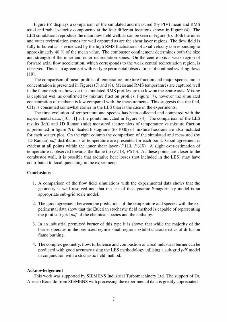
Figure (6) displays a comparison of the simulated and measured (by PIV) mean and RMSaxial and radial velocity components at the four different locations shown in Figure (4). TheLES simulations reproduce the main flow field well, as can be seen in Figure (6). Both the innerand outer recirculation zones are well captured as are the shear layer regions. The flow field isfully turbulent as is evidenced by the high RMS fluctuations of axial velocity corresponding toapproximately 40 % of the mean value. The combustor confinement determines both the sizeand strength of the inner and outer recirculation zones. On the centre axis a weak region offorward axial flow acceleration, which corresponds to the weak central recirculation region, isobserved. This is in agreement with early experimental observations of confined swirling flows[19].

The comparison of mean profiles of temperature, mixture fraction and major species molarconcentration is presented in Figures (7) and (8). Mean and RMS temperatures are captured wellin the flame regions, however the simulated RMS profiles are too low on the centre axis. Mixingis captured well as confirmed by mixture fraction profiles, Figure (7), however the simulatedconcentration of methane is low compared with the measurements. This suggests that the fuel,CH4 is consumed somewhat earlier in the LES than is the case in the experiments.

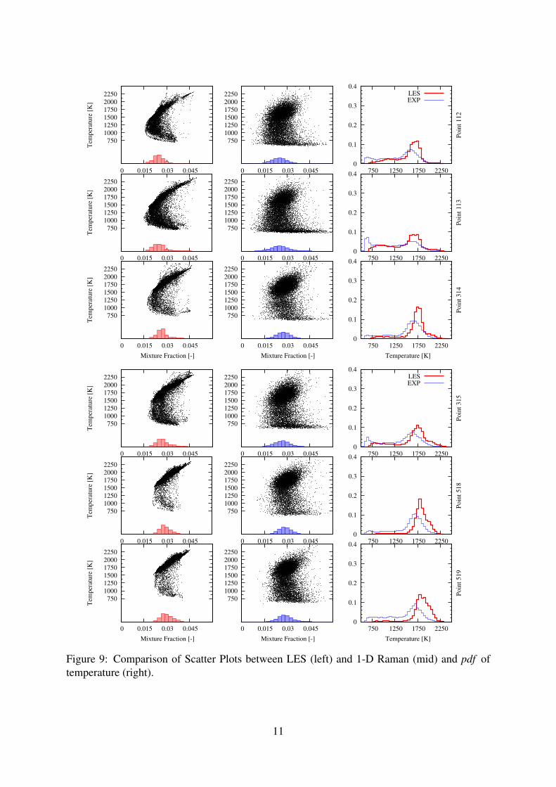
The time evolution of temperature and species has been collected and compared with theexperimental data, [10, 11] at the points indicated in Figure (4). The comparison of the LESresults (left) and 1D Raman (mid) measured scatter plots of temperature vs mixture fractionis presented in figure (9). Scaled histograms (to 1000) of mixture fractions are also includedfor each scatter plot. On the right column the comparison of the simulated and measured (by1D Raman) pdf distributions of temperature are presented for each point. Good agreement isevident at all points within the inner shear layer (P113, P315). A slight over-estimation oftemperature is observed towards the flame tip (P518, P519). As these points are closer to thecombustor wall, it is possible that radiative heat losses (not included in the LES) may havecontributed to local quenching in the experiments.

Conclusions

1. A comparison of the flow field simulations with the experimental data shows that thegeometry is well resolved and that the use of the dynamic Smagorinsky model is anappropriate sub-grid scale model.

2. The good agreement between the predictions of the temperature and species with the ex-perimental data show that the Eulerian stochastic field method is capable of representingthe joint sub-grid pdf of the chemical species and the enthalpy.

3. In an industrial premixed burner of this type it is shown that while the majority of theburner operates in the premixed regime small regions exhibit characteristics of diffusionflame burning.

4. The complex geometry, flow, turbulence and combustion of a real industrial burner can bepredicted with good accuracy using the LES methodology utilising a sub-grid pdf modelin conjunction with a stochastic field method.

AcknowledgementThis work was supported by SIEMENS Industrial Turbomachinery Ltd. The support of Dr.

Alessio Bonaldo from SIEMENS with processing the experimental data is greatly appreciated.

7

(a) Axial Velocity. Mean on top, RMS at the bottom.

(b) Radial Velocity. Mean on top, RMS at the bottom.

Figure 6: Comparison of Axial and Radial Velocity profiles.

8

(a) Mixture Fraction. Mean on top, RMS at the bottom.

(b) Temperature. Mean on top, RMS at the bottom.

Figure 7: Comparison of Temperature and Mixture Fraction profiles.

9

(a) Methane Mass Fraction. Mean on top, RMS at the bottom.

(b) CO2 Mass Fraction. Mean on top, RMS at the bottom.

Figure 8: Comparison of Methane and CO2 Mass Fraction profiles.

10

750

1000

1250

1500

1750

2000

2250

0 0.015 0.03 0.045

Tem

per

atu

re [

K]

750

1000

1250

1500

1750

2000

2250

0 0.015 0.03 0.045 0

0.1

0.2

0.3

0.4

750 1250 1750 2250

Po

int

11

2

LESEXP

750

1000

1250

1500

1750

2000

2250

0 0.015 0.03 0.045

Tem

per

atu

re [

K]

750

1000

1250

1500

1750

2000

2250

0 0.015 0.03 0.045 0

0.1

0.2

0.3

0.4

750 1250 1750 2250

Po

int

11

3

750

1000

1250

1500

1750

2000

2250

0 0.015 0.03 0.045

Tem

per

atu

re [

K]

Mixture Fraction [-]

750

1000

1250

1500

1750

2000

2250

0 0.015 0.03 0.045

Mixture Fraction [-]

0

0.1

0.2

0.3

0.4

750 1250 1750 2250

Po

int

31

4

Temperature [K]

750

1000

1250

1500

1750

2000

2250

0 0.015 0.03 0.045

Tem

per

atu

re [

K]

750

1000

1250

1500

1750

2000

2250

0 0.015 0.03 0.045 0

0.1

0.2

0.3

0.4

750 1250 1750 2250P

oin

t 3

15

LESEXP

750

1000

1250

1500

1750

2000

2250

0 0.015 0.03 0.045

Tem

per

atu

re [

K]

750

1000

1250

1500

1750

2000

2250

0 0.015 0.03 0.045 0

0.1

0.2

0.3

0.4

750 1250 1750 2250

Po

int

51

8

750

1000

1250

1500

1750

2000

2250

0 0.015 0.03 0.045

Tem

per

atu

re [

K]

Mixture Fraction [-]

750

1000

1250

1500

1750

2000

2250

0 0.015 0.03 0.045

Mixture Fraction [-]

0

0.1

0.2

0.3

0.4

750 1250 1750 2250

Po

int

51

9

Temperature [K]

Figure 9: Comparison of Scatter Plots between LES (left) and 1-D Raman (mid) and pdf oftemperature (right).

11

References[1] L. Valino. A field Monte Carlo formulation for calculating the probability density function

of a single scalar in a turbulent flow. Flow, Turbulence and Combustion, 60(2):157–172,1998.

[2] V. Sabel’nikov and O. Soulard. Rapidly decorrelating velocity-field model for as a tool forsolving one point Fokker-Planck equations for probability density functions of turbulentreactive scalars. Physial Review E, 72(1):016301, 2005.

[3] C. Gardiner. Handbook of Stochastic Methods. Springer Verlag, 1985.[4] W. P. Jones and A. Tyliszczak. Large eddy simulation of spark ignition in a gas turbine

combustor. Flow Turbulence Combust., 85:711–734, 2010.[5] W. P. Jones and V. N. Prasad. LES-pdf of a spark ignited turbulent methane jet. Proceed-

ings of The Combustion Institute, 2011. in press.[6] W. P. Jones and S. Navarro-Martinez. Large eddy simulations of autoignition with a sub-

grid probability density method. Combustion and Flame, 150(3):170–187, 2007.[7] W. P. Jones and S. Navarro-Martinez. Study of hydrogen auto-ignition in a turbulent air

co-flow using large eddy simulation approach. Computers & Fluids, 37:802–808, 2007.[8] W. P. Jones and V. N. Prasad. Large eddy simulation of the Sandia flame series (D-F)

using the Eulerian stochastic field method. Combustion and Flame, 157(9):1621–1636,2010.

[9] V.N. Prasad. Large Eddy Simulation of partially premixed turbulent combustion. PhDthesis, Imperial College, University of London, 2011.

[10] U.Stopper, M. Aigner, W. Meier, R. Sadanandan, M. Stor, and I.S. Kim. Flow field andcombustion characterisation of premixed gas turbine flames by planar laser techniques.Journal of Engineering for Gas Turbines and Power, 131(2), 2009.

[11] U.Stopper, M. Aigner, H. Ax, W. Meier, R. Sadanandan, M. Stor, and A. Bonaldo. PIV,2D-LIF, and 1-D raman measurements of flow field, composition and temperature in pre-mixed gas turbine flames. Experimental Thermal and Fluid Science, 34(3), 2010.

[12] U. Piomelli and J. Liu. Large eddy simulation of rotating channel flows using a localiseddynamic model. Physics of Fluids, 7(4):839–848, 1995.

[13] F. Gao and E. O’Brian. A large-eddy simulation scheme for turbulent reacting flows.Physics of Fluids A, 5:1282–1284, 1993.

[14] C. Dopazo. Relaxation of initial probability density functions in the turbulent convectionof scalar fields. Physics of Fluids, 22(1):20–30, 1979.

[15] Radu Mustata, Luis Valino, Carmen Jimenez, W. P. Jones, and S. Bondi. A probabilitydensity function Eularian Monte-Carlo field method for large eddy simulations: Applica-tion to a turbulent piloted methane/air diffusion flame (sandia d). Combustion and Flame,145:88–104, 2006.

[16] C. J. Sung, C. K. Law, and J. Y. Chen. Augmented reduced mechanisms for no emissionin methane oxidation. Combustion and Flame, 125(906-919), 2001.

[17] T. Sarpkaya. On stationary and travelling vortex breakdowns. Journal of Fluid Mechanics,45(3):545–559, 1971.

[18] Y. Mizobuchi, S. Tachibana, J. Shinio, S. Ogawa, and T. Takeno. A numerical analysisof the structure of a turbulent hydrogen jet lifted flame. Proceedings of The CombustionInstitute, 29(1):2009–2015, 2002.

[19] N. Syred and J. M. Beer. Combustion in swirling flows: a review. Combustion and Flame,23:143–201, 1974.

12