lax algebras — a scenic approach
TRANSCRIPT

Lax Algebras — A Scenic Approach
Christoph Schubert
Dissertation
zur Erlangung des Grades eines Doktors derNaturwissenschaften
– Dr. rer. nat. –
Vorgelegt im Fachbereich 3 (Mathematik & Informatik)der Universitat Bremen
im Oktober 2006
Datum des Promotionskolloquiums: 1. Dezember 2006
Erster Gutachter: Prof. Dr. H.-E. Porst, Universitat BremenZweiter Gutachter: Prof. Dr. W. Tholen, York University, Toronto
Contents
Introduction 7The setting . . . . . . . . . . . . . . . . . . . . . . . . . . . . . . . . . . . . 8Overview . . . . . . . . . . . . . . . . . . . . . . . . . . . . . . . . . . . . . 9Acknowledgments . . . . . . . . . . . . . . . . . . . . . . . . . . . . . . . . . 11Conventions . . . . . . . . . . . . . . . . . . . . . . . . . . . . . . . . . . . . 12
1 Ordered categories 131.1 Morphisms for ordered categories, free ordered categories . . . . . . . . 141.2 Maps and special ordered categories . . . . . . . . . . . . . . . . . . . . 161.3 Kock–Zoberlein monads . . . . . . . . . . . . . . . . . . . . . . . . . . 23
1.3.1 Downsets and upsets . . . . . . . . . . . . . . . . . . . . . . . . 241.3.2 Finitely generated downsets . . . . . . . . . . . . . . . . . . . . 251.3.3 Non-empty downsets . . . . . . . . . . . . . . . . . . . . . . . . 251.3.4 Ideals and filters . . . . . . . . . . . . . . . . . . . . . . . . . . 251.3.5 Kleisli categories . . . . . . . . . . . . . . . . . . . . . . . . . . 261.3.6 Distributive laws and composite monads . . . . . . . . . . . . . 27
1.4 Quantaloids . . . . . . . . . . . . . . . . . . . . . . . . . . . . . . . . . 311.4.1 Biproducts . . . . . . . . . . . . . . . . . . . . . . . . . . . . . . 31
1.5 Examples . . . . . . . . . . . . . . . . . . . . . . . . . . . . . . . . . . 331.5.1 Relations in regular categories . . . . . . . . . . . . . . . . . . . 331.5.2 V-Matrices . . . . . . . . . . . . . . . . . . . . . . . . . . . . . 38
1.6 Pre-scenes . . . . . . . . . . . . . . . . . . . . . . . . . . . . . . . . . . 431.6.1 (S,O)-categories . . . . . . . . . . . . . . . . . . . . . . . . . . 441.6.2 (S,O)-distributors . . . . . . . . . . . . . . . . . . . . . . . . . 461.6.3 Duality for O-categories and O-groupoids . . . . . . . . . . . . 481.6.4 Kleisli pre-scenes . . . . . . . . . . . . . . . . . . . . . . . . . . 49
2 Scenes and actors 552.1 Scenes . . . . . . . . . . . . . . . . . . . . . . . . . . . . . . . . . . . . 55
2.1.1 Examples . . . . . . . . . . . . . . . . . . . . . . . . . . . . . . 562.2 Morphisms for scenes and actors . . . . . . . . . . . . . . . . . . . . . . 58
2.2.1 Scenes vs. pre-scenes . . . . . . . . . . . . . . . . . . . . . . . . 622.3 Constructing actors . . . . . . . . . . . . . . . . . . . . . . . . . . . . . 62
2.3.1 Taut functors . . . . . . . . . . . . . . . . . . . . . . . . . . . . 632.3.2 Constructing actors on D . . . . . . . . . . . . . . . . . . . . . 68
3
4 Contents
2.3.3 Constructing actors on MatV . . . . . . . . . . . . . . . . . . . 712.3.4 From Dist to OrdMatV . . . . . . . . . . . . . . . . . . . . . . 782.3.5 Extending functors to Kleisli categories . . . . . . . . . . . . . . 79
2.4 Some conditions on scenes . . . . . . . . . . . . . . . . . . . . . . . . . 85
3 Lax algebras 873.1 Basics . . . . . . . . . . . . . . . . . . . . . . . . . . . . . . . . . . . . 87
3.1.1 First examples . . . . . . . . . . . . . . . . . . . . . . . . . . . 883.2 Faithful fibrations . . . . . . . . . . . . . . . . . . . . . . . . . . . . . . 893.3 Lax algebras are universal . . . . . . . . . . . . . . . . . . . . . . . . . 92
3.3.1 Change of base . . . . . . . . . . . . . . . . . . . . . . . . . . . 923.3.2 The construction . . . . . . . . . . . . . . . . . . . . . . . . . . 933.3.3 Conclusions . . . . . . . . . . . . . . . . . . . . . . . . . . . . . 95
3.4 Lax algebras for a monad . . . . . . . . . . . . . . . . . . . . . . . . . 953.4.1 Topological spaces and approach spaces: the motivating example 973.4.2 Further examples . . . . . . . . . . . . . . . . . . . . . . . . . . 993.4.3 The embeddings Alg∗T −→ Alg T . . . . . . . . . . . . . . . . 1013.4.4 Ordering morphisms . . . . . . . . . . . . . . . . . . . . . . . . 104
3.5 Strict and costrict morphisms . . . . . . . . . . . . . . . . . . . . . . . 1053.5.1 Examples . . . . . . . . . . . . . . . . . . . . . . . . . . . . . . 1053.5.2 Basic properties . . . . . . . . . . . . . . . . . . . . . . . . . . . 1083.5.3 Strict and costrict morphisms transfer transitivity . . . . . . . . 110
3.6 Quotients and descent . . . . . . . . . . . . . . . . . . . . . . . . . . . 1113.6.1 Quotients and regular epimorphisms of lax algebras . . . . . . . 1113.6.2 Descent morphisms . . . . . . . . . . . . . . . . . . . . . . . . . 1133.6.3 Descent for lax algebras . . . . . . . . . . . . . . . . . . . . . . 115
3.7 Change of theory . . . . . . . . . . . . . . . . . . . . . . . . . . . . . . 1163.7.1 Examples . . . . . . . . . . . . . . . . . . . . . . . . . . . . . . 1183.7.2 Change of base revisited . . . . . . . . . . . . . . . . . . . . . . 121
4 Further examples 1234.1 Comparing Kleisli-scenes and distributors . . . . . . . . . . . . . . . . . 1234.2 Level algebras and tower-extensions . . . . . . . . . . . . . . . . . . . . 1264.3 An example: topological spaces via filter convergence . . . . . . . . . . 131
4.3.1 Extending the filter-functor to Dist . . . . . . . . . . . . . . . . 1314.3.2 Other topological constructs via filter convergence . . . . . . . . 132
4.4 Back to Kleisli . . . . . . . . . . . . . . . . . . . . . . . . . . . . . . . . 1334.4.1 An example: closure spaces via neighborhoods . . . . . . . . . . 1344.4.2 Algebraic closure spaces . . . . . . . . . . . . . . . . . . . . . . 1354.4.3 Grounded closure spaces . . . . . . . . . . . . . . . . . . . . . . 136
4.5 The filter construction . . . . . . . . . . . . . . . . . . . . . . . . . . . 1364.5.1 Quasi-uniform spaces . . . . . . . . . . . . . . . . . . . . . . . . 139

Contents 5
5 Partial morphisms 1435.1 Generalities . . . . . . . . . . . . . . . . . . . . . . . . . . . . . . . . . 1435.2 Representing initial morphisms . . . . . . . . . . . . . . . . . . . . . . 1455.3 Representing strict and costrict morphisms . . . . . . . . . . . . . . . . 148
5.3.1 Costrict morphisms . . . . . . . . . . . . . . . . . . . . . . . . . 1495.3.2 Strict morphisms . . . . . . . . . . . . . . . . . . . . . . . . . . 150
5.4 Examples . . . . . . . . . . . . . . . . . . . . . . . . . . . . . . . . . . 1515.5 Some applications . . . . . . . . . . . . . . . . . . . . . . . . . . . . . . 152
5.5.1 Subobject classifier and T0-objects . . . . . . . . . . . . . . . . 1535.5.2 Exponentiability . . . . . . . . . . . . . . . . . . . . . . . . . . 153
6 More on limits and colimits 1556.1 Coproducts . . . . . . . . . . . . . . . . . . . . . . . . . . . . . . . . . 155
6.1.1 Coproducts in categories of lax algebras . . . . . . . . . . . . . 1556.1.2 The frame of a lax algebra . . . . . . . . . . . . . . . . . . . . . 1586.1.3 Extensivity . . . . . . . . . . . . . . . . . . . . . . . . . . . . . 159
6.2 Local cartesian closedness . . . . . . . . . . . . . . . . . . . . . . . . . 161
7 Compactness 1657.1 Topology in a (finitely) complete category . . . . . . . . . . . . . . . . 1657.2 A Tychonoff Theorem . . . . . . . . . . . . . . . . . . . . . . . . . . . 167
7.2.1 Stable topologies for lax algebras . . . . . . . . . . . . . . . . . 1687.2.2 Pullback-modular scenes . . . . . . . . . . . . . . . . . . . . . . 169
7.3 Factorization systems and closure operators . . . . . . . . . . . . . . . 171
6 Contents
Introduction
In this thesis we propose scenes as a setting for the study of lax algebras.Lax algebras are a 2-categorical generalization of Eilenberg–Moore algebras for a
monad. It is well-known that categories of Eilenberg–Moore algebras convenientlydescribe algebraic categories. Lax algebras provide a framework for studying differenttopological categories simultaneously.
The best way to illustrate this might be to recall the motivating example of [Bar70].In [Man69] Manes showed that the category SetU of Eilenberg–Moore algebras for
the ultrafilter monad U = (U, e,m) on the category Set of sets and functions is thecategory of compact Hausdorff topological spaces and continuous maps. Intuitively, onecan understand his result as follows. Recall that in a compact Hausdorff topologicalspace every ultrafilter has a unique convergence point. Thus each compact Hausdorfftopological space with underlying set X gives rise to a function c : UX −→ X, whichsends each ultrafilter to its convergence point. Remarkably, the functions c which arisein this way are precisely those which satisfy c · eX = 1X and c · Uc = c ·mX , that is,those which turn (X, c) into an Eilenberg–Moore algebra for U.
For an arbitrary topological space we loose existence and uniqueness of convergencepoints, but we still have a convergence relation k ⊂ UX×X. Barr [Bar70] characterizedthe relations k that arise as convergence relation of a topological space as those whichsatisfy
1X ⊂ k · eX and k · Uk ⊂ k ·mX . (I.1)
Here U is an extension of the functor U to the category Rel of sets and relations.Of course, the inclusion (I.1) are meaningful for any monad U on Set which has anextension to Rel. Hence, it is now possible to define relational algebras for any monadon Set with an extension to Rel.
For a while, Barr’s result sparked only modest interest. In [Bun74] the question ofhow to construct extensions of monads is addressed; [Kam74] and [Mob81] generalizeBarr’s definition to relations in regular categories and to relations with respect to asuitable factorization system in a category. But the development of the theory washindered by the fact that there was a certain lack of examples: essentially the onlyother category which was presented as a category of lax algebras was the category Ordof (pre-)ordered sets and monotone functions, which stems from the identity monad onSet.
But ultrafilter convergence was used profitably in [RT94] to describe effective descentmorphisms of topological spaces, and in [Pis99] to characterize exponentiable topolog-ical spaces. This led Clementino and Hofmann [CH03] to start a new line of research
7

8 Introduction
on relational algebras.
The setting of [CH03] is no longer a category together with a notion of relationderived from it by, for instance, a factorization system. Rather, it is a category whichsits inside a 2-category with thin hom-categories, that is, between any parallel pair of1-cells there is at most one 2-cell. This generalization opened the possibility to includeLawvere’s generalized metric spaces [Law73], Lowen’s approach spaces [Low97], as wellas quasi-uniform spaces among the examples of relational algebras in this generalizedsense; or lax algebras, as the objects of study were subsequently called.
In [CH03] some attention is payed to structures which only need to satisfy the lefthand inequality of (I.1), and to structures which do not satisfy any inequality of (I.1)at all. In general, the so-defined supercategories of the category of lax algebras havebetter convenience properties. It is thus possible to perform many constructions in thesupercategories, and then reflect them down to the category of lax algebras in question.
Incorporating metrics and approach structures was facilitated by using the matrixconstruction of [BCSW83], where the matrices take values in a quantale V. In subse-quent articles, as for example, [CHT03b], [CHT04], and [CH04a], the setting is special-ized to the category V-matrices.
The setting
The work that is presented here can be seen as a continuation of [CH03]. Indeed,the setting of [CH03] is essentially equivalent to what we choose to call pre-scenes.This setting has the advantage that it is general enough to capture all the topologicalexamples of lax algebras that were studied so far. At the same time our setting is sorestricted that we do not have to bother with coherence-questions, cf. [CT03]. But weloose the possibility to capture (non-thin) categories and multi-categories, as in [CT03]and [CHT03b].
A pre-scene can be seen as an ordered category with a class of maps with chosenright adjoints. That is, we will work in a category O enriched over the cartesian closedcategory Ord. In such a category, we can speak about (right) adjoints: f ∗ : Y −→ Xis right adjoint to f : X −→ Y in O if 1X ≤ f ∗ · f and f · f ∗ ≤ 1Y hold in O. We callf ∈ O a map if there exists some f ∗ right adjoint to f . The notion, due to Lawvere,is motivated by the following observation: in the ordered category Rel of sets andrelations, a morphisms has a right adjoint if and only if it is the graph of a function.
For studying lax algebras, we find it convenient to introduce some more structureon pre-scenes, leading to scenes. These scenes, together with an appropriate notion ofmorphism, are the basis for our notion of lax algebras.
We are now going to briefly describe the contents of this work:
Overview 9
Overview
Chapter 1 This chapter is an introduction to order-enriched category theory. Sinceany order-enriched category is in particular a 2-category, we can use the language andtools from higher-dimensional category theory. For the reader’s convenience and tosettle the notation, we include all the necessary details.
After introducing basic definitions concerning order-enriched (or ordered) categories,we define different types of morphisms of ordered categories and construct the freeordered category over a category with specified relations between parallel morphisms.
We define what we call a map in an ordered category and demonstrate some simpleproperties of maps. After that, we introduce the notion of a Beck–Chevalley squareand some modularity laws which are crucial to a more refined study of lax algebras.
Kock–Zoberlein monads are introduced and some examples are discussed. Then werecall distributive laws between monads and introduce quantaloids and biproducts.
We present two important classes of examples of ordered categories: categories ofrelations for a regular category and matrices with values in a quantale. Using theseexamples we illustrate the notions introduced so far.
We define pre-scenes and associate to any pre-scene O an ordered category CatO
of O-categories and O-functors. As a first example, we obtain the category Ord ofordered sets and monotone functions as CatO for a simple pre-scene O. Taking Ordas a guiding example, we develop some basic notions of O-categories.
Suitable monads on Ord give rise to pre-scenes by the Kleisli-construction. As anexample, we consider an extension of the familiar filter-monad on Set to Ord. Forthis monad, the categories of the corresponding pre-scene are precisely the topologicalspaces. Then we introduce a notion of fuzzy powerset with values in a quantale V andshow that the category of V-matrices considered before is the Kleisli-category for theV-valued fuzzy powerset monad.
Chapter 2 Here we introduce scenes as a natural environment to study lax algebras,and present some examples, like (C, RelC) for a regular category C and (Set, MatV)for a quantale V, as well as scenic functors or morphisms of scenes.
Lax algebras will be defined with respect to a scene S and an actor on it, that is, ascenic functor S −→ S. This actor takes the role of (the extension of) the ultrafilterfunctor in Barr’s example.
After a discussion of taut [Man02] functors and the filter-functor, we describe variousways of constructing actors by extending a base-functor.
One method of construction for extensions of functors, which has not been used sofar in the lax algebra-community, is the use of distributive laws to construct extensionsto Kleisli categories. We give an elementary proof — which we could not find in theliterature — of the correspondence between distributive laws and extensions.
In the last section of Chapter 2 we fix some useful notation concerning scenes.
10 Introduction
Chapter 3 The central topic of this thesis is introduced: the category Alg T of laxalgebras for an actor T on a scene. We discuss some examples and show that thecanonical forgetful functor of a category of lax algebras is both a fibration and anopfibration, thus is a fibering in the sense of [Man67]. We recall some basic facts aboutfiberings.
Using the free ordered category construction from Chapter 1, we prove a repre-sentation theorem for fiberings: Every fibering arises as a category of lax algebras.Unfortunately, this representation theorem is of little use. We are not aware of a singlefact about any fibering which can be proved with its help.
For this reason we now start to study subcategories of Alg T defined with the helpof a monad structure T = (T, e,m) on T . This leads us to a string
AlgtT ↪−→ AlguT ↪−→ AlgrT ↪−→ Alg T (I.2)
of concrete full inclusions. We present the paradigmatic example of Barr [Bar70] andits extension due to Clementino and Hofmann [CH03]: For T the suitably extendedultrafilter monad on Set, diagram (I.2) becomes
Top ↪−→ PrTop ↪−→ PsTop ↪−→ URS.
Here Top is the category of topological spaces, PrTop and PsTop are the categoriesof pre- and pseudo-topological spaces, respectively, and URS is the category of ultra-relational spaces.
After presenting some examples of lax algebras, we continue to study the embeddingsin (I.2) and give conditions under which they are reflective.
We introduce strict and costrict morphisms of lax algebras, which generalize properand open continuous functions between topological spaces.
We continue with a description of quotients in some of the categories of (I.2). Thisleads to some results on descent morphisms in the above categories, by methods whichare an adaption of the ones used in [CH04a]. As a corollary, we obtain that proper andopen surjections in Top are effective descent morphisms.
Then we describe how concrete functors between categories of lax algebras are in-duced by transformations between their actors.
Chapter 4 In this chapter we present more examples of categories of lax algebras.For a suitable monad T on Ord, we compare the categories of the Kleisli pre-scene ofT to the lax algebras for the extension of T to the scene of distributors.
We make explicit the connection between Zhang’s tower extensions and lax algebrasdefined over the scene (Set, MatV) for quantale V: we show that lax algebras over(Set, MatV) provide an intrinsic description of the tower extension “by V” of algebrasover (Set,Rel).
We finally present the first “non-generic” example of this chapter, namely topologicalspaces via filter convergence.
Acknowledgments 11
Using our results on tower extensions, we present (pre-)approach and probabilistictopological spaces as lax algebras via filter convergence. Following an idea of Seal[Sea05b], we show how closure spaces arise as categories for a pre-scene. Next, wediscuss how algebraic and grounded closure spaces arise as lax algebras. We close thischapter with some results on (quasi-)uniform spaces.
Chapter 5 We continue with a study of exactness properties of categories of laxalgebras. First, we study the representability of partial morphisms in categories of laxalgebras. This can indeed be seen as a (very weak) exactness property, cf. [AHS04].
Using the strict and costrict morphisms introduced in Chapter 3, we recover theresults of Brown on representability of closed- and open-embedding partial morphismsin Top. Finally, using results of Dyckhoff and Tholen, we use our results on partialmorphisms to deduce Niefield’s result on exponentiability of locally-closed embeddingsin Top.
Chapter 6 We extend the material from [MST06] on the structure of coproductsin categories of lax algebras; coproducts are characterized using costrict morphisms.Thus, again costrict morphisms play a crucial role. Under additional completenessconditions, we construct a functor from Alg T to the category Loc of locales. Here weassociate to every lax algebra its frame of costrict subalgebras. In case one works overSet, this yields a concrete, coproduct-preserving functor into Top.
Using the above-mentioned characterization of coproducts in categories of lax alge-bras, we give conditions for the extensivity of these categories.
We construct, under suitable conditions, partial products in Alg T , and thus estab-lish that Alg T is locally cartesian closed.
The chapter ends with some remarks on quasitopoi of lax algebras.
Chapter 7 We use the approach of Clementino, Giuli, and Tholen to “topology ina category” to study compactness of lax algebras. Under suitable conditions, everycategory of lax algebras comes with a canonical topology, given by the strict morphisms.Often this topology turns out to be what we choose to call stable, that is, closedunder wide pullbacks. This allows us to prove (infinitary) Tychonoff and Frolık-typetheorems for these lax algebras. As a corollary we obtain the well-known results aboutcompactness of topological spaces and about 0-compactness of approach spaces. Thematerial in this chapter is an extension of [Sch05].
We use closedness of strict embeddings under intersection to define a categoricalclosure operator on Alg T .
Acknowledgments
First of all, I would like to thank my supervisor Hans-Eberhard Porst for his support.
12 Introduction
A three-year scholarship from the Ernst A.-C. Lange Stiftung in Bremen and thesupport of the Zentrale Forschungsforderung of the Universitat Bremen on variousoccasions are gratefully acknowledged.
I owe special thanks to Walter Tholen for his continued interest in my work. Hiscriticism and suggestions had a profound impact on my direction of research and on thepresentation of the results. I also have to thank him for his invitations to York Univer-sity and for financial support (through NSERC). Without my stay at York University,this work and my life would look quite different.
The hospitality of the mathematics departments of Stellenbosch University, Stellen-bosch, South Africa, and of York University, Toronto, Canada, is gratefully acknowl-edged. I especially thank Barry Green and David Holgate from Stellenbosch University.
During the past years I have profited greatly from remarks and questions fromMaria Manuel Clementino, Bjorn Gohla, Horst Herrlich, Dirk Hofmann, David Hol-gate, George Janelidze, Lutz Schroder, and, in particular, Gavin Seal.
Special thanks go to my parents for all their love and support.Last but not least, I would like to thank my wife Ana Paola Sanchez Lezama for
being precisely how she is.
Conventions
The end of a proof will be marked by . In case we do not see any need for a detailedproof, either because it would consist out of straightforward calculations or it is includedin the preceding discussion, will directly follow the statement of the result.
For categorical terminology we refer to [AHS04].

1 Ordered categories
Convention An ordered set will always be a set equipped with a reflexive and tran-sitive relation. Hence ordered set and thin small category are synonymous terms. Thecategory of ordered sets and monotone functions will be denoted by Ord. We willfreely use the notions and notation introduced in [Woo04], which gives a beautifulintroduction to ordered sets.
Given x, y in an ordered set (X,≤) we write
x ≈ y if and only if x ≤ y and y ≤ x.
An ordered set is called separated (or antisymmetric, skeletal) if x ≈ y implies x = y.An ordered category O is a locally thin 2-category. That is, the “hom-categories”
O(A,B) are just ordered sets. Alternatively, we may view an ordered category as acategory enriched over the cartesian closed category Ord.
Put into elementary terms, this means that an ordered category O is given by an“ordinary” category O such that for each pair (A,B) of O-objects we have an order onthe collection O(A,B), and these orders are compatible in the sense that g ≤ g impliesh · g · f ≤ h · g · f for all
Af
�� Bg
��
g��C
h �� D
in O. We will refer to instances g ≤ g of the orders as 2-cells. Any ordered category hasan underlying category, obtained by forgetting the 2-cells (order-relations), and also anunderlying 2-graph (see [Str96]), obtained by forgetting composition and identities.
The primordial example of an ordered category is Rel, the 2-category which has setsas objects and relations as morphisms. If r : A −→ B and s : B −→ C are morphismsin Rel, that is, if r ⊂ A×B and s ⊂ B × C, then
s · r := { (a, c) ∈ A× C | ∃b ∈ B : (a, b) ∈ r, (b, c) ∈ s }.
2-cells are given by inclusion.Another important example is the category Ord itself, where a 2-cell f ≤ g exists
for f, g : (X,≤) −→ (Y,≤) iff f(x) ≤ g(x) holds for all x ∈ X. Any topologicalspace X has an underlying ordered set, given by the generalization order : x ≤ y iffthe principal ultrafilter x converges to y, equivalently, y ∈ cl{x}. This order is thedual of the well-known specialization order [GHK+03, O-5.2.]. They are antisymmetricprecisely when the space is T0. Obviously, any continuous mapping is monotone with
13

14 1 Ordered categories
respect to the generalization orders, and we can consider Top as an ordered categoryby pointwise generalization order.
We call a morphism f : X −→ Y in an ordered category O order-monic if m·x ≤ m·yimplies x ≤ y for each parallel pair x, y in O. In Ord, a monotone function f : (X,≤) −→ (Y,≤) is order-monic iff f is fully-faithful , that is, f(x) ≤ f(x′) ⇐⇒ x ≤ x′
holds for all x, x′ ∈ X (cf. [Woo04])If P is any property of ordered sets, we say an ordered category O locally has P pro-
vided O(A,B) has P for all O-objects A, B. So, for instance, Rel is locally separatedwhile Ord is not locally separated.
For an ordered category O, we can not only form the dual ordered category Oop by“turning around the 1-cells”, but also the conjugate ordered category Oco by “turningaround the 2-cells”: g ≤ f in Oco iff f ≤ g in O. Of course, these can be combined,and Ocoop = Oopco holds for any O.
1.1 Morphisms for ordered categories, free ordered categories
When it comes to morphisms of ordered categories, there a several notions we canconsider. The following 2-categorical concepts are well-known; see for instance [Str96]or [Bor94]. Nonetheless, we repeat them here for the reader’s convenience and tosettle notation. We will frequently use the notion of 2-graph morphism between (theunderlying 2-graphs) of ordered categories: Given ordered categories O and P, a 2-
graph morphism OG−→ P assigns to every O-object A a P-object GA, to every O-
morphism Af−→ B a P-morphism GA
Gf−→ GB, and to every 2-cell f ≤ f in O a 2-cell
Gf ≤ Gf in P. Observe that, due to the scarcity of 2-cells in O and P, G alreadypreserves all the structure on the level of 2-cells. In particular, for any pair (A,B) ofO-objects we get a restriction
GAB : O(A,B) −→ P(GA,GB),
which is monotone. Thus whenever P is a property of monotone functions, we will saythat G has locally P provided GAB has P for all O-objects A, B. For example, G iscalled locally fully-faithful (or 2-full) if Gf ≤ Gf implies f ≤ f .
Definition 1.1.1 Let O and P be ordered categories and OG−→ P be a 2-graph
morphism. We say that G is
(1) a 2-functor if G is a functor between the underlying categories of O and P;
(2) a pseudo-functor if F preserves composition and identities up to ≈; that is, Gg ·Gf ≈ G(g · f) and 1GA ≈ G1A hold,
(3) a lax functor if Gg ·Gf ≤ G(g · f) and 1GA ≤ G1A hold,

1.1 Morphisms for ordered categories, free ordered categories 15
(4) an oplax functor if G(g · f) ≤ Gg ·Gf and G1A ≤ 1GA hold,
whenever the compositions are defined in O. Moreover, we call G normal if G1A ≈ 1GA
holds for all A.
Next we generalize natural transformations to our “relaxed” setting:
Definition 1.1.2 Let O and P be ordered categories and F,G : O −→ P 2-graph
morphisms. A transformation Fλ−→ G is given by a family (FO
λO−→ FO)O∈objO ofP-morphisms. We call such a λ a
(1) pseudo-natural transformation provided
FAλA ��
≈Ff
��
GA
Gf
��
FBλB
�� GB
that is, Gf · λA ≈ λB · Ff , holds for any Af−→ B in O;
(2) lax transformation provided Gf · λA ≤ λB · Ff holds for any Af−→ B in O;
(3) oplax transformation provided λB · Ff ≤ Gf · λA holds for any Af−→ B in O.
We write OrdCat for the category of ordered categories and pseudo-functors andOrdCats for the (non-full) subcategory of OrdCat given by the 2-functors.
Free ordered categories The construction of free ordered categories is extremelyeasy. This is due to the fact that the existence of a 2-cell f ≤ g is a mere property ofthe pair (f, g).
Definition 1.1.3 A locally related category is a pair (C, τ), consisting of a categoryC together with family of relations (τAB)(A,B)∈(objC)2 with τAB ⊂ C(A,B)2 for allA,B. A morphism of locally related categories F : (C, τ) −→ (C′, τ ′) is given bya functor F : C −→ C′ which locally preserves τ in the sense that fτABg impliesF (f)τ ′
F (A)F (B)F (g). We write lrCat for the category of (small) locally related categoriesand their morphisms.
We have the obvious forgetful functors
OrdCatsU ��
�������
�����
lrCat
V�����������
Cat.
Clearly V has a left adjoint, which equips any category C with τAB = ∅.
16 1 Ordered categories
Proposition 1.1.4 U : OrdCats −→ lrCat has a concrete left adjoint O.
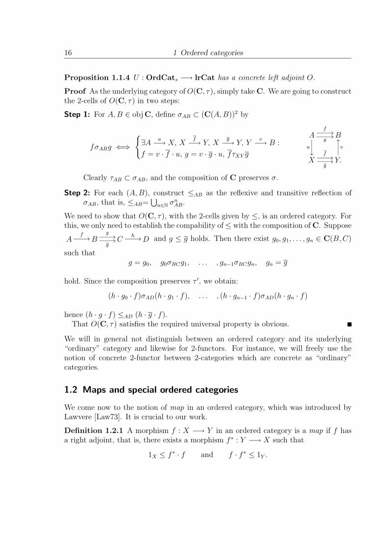
Proof As the underlying category of O(C, τ), simply take C. We are going to constructthe 2-cells of O(C, τ) in two steps:
Step 1: For A,B ∈ objC, define σAB ⊂ (C(A,B))2 by
fσABg ⇐⇒
{∃A
u−→ X, X
f−→ Y, X
g−→ Y, Y
v−→ B :
f = v · f · u, g = v · g · u, fτXY g
Af
��
g��
u
��
B
Xf
��
g�� Y.
v
��
Clearly τAB ⊂ σAB, and the composition of C preserves σ.
Step 2: For each (A,B), construct ≤AB as the reflexive and transitive reflection ofσAB, that is, ≤AB=
⋃n∈N σn
AB.
We need to show that O(C, τ), with the 2-cells given by ≤, is an ordered category. Forthis, we only need to establish the compability of ≤ with the composition of C. Suppose
Af
�� Bg
��
g�� C
h �� D and g ≤ g holds. Then there exist g0, g1, . . . , gn ∈ C(B,C)
such thatg = g0, g0σBCg1, . . . , gn−1σBCgn, gn = g
hold. Since the composition preserves τ ′, we obtain:
(h · g0 · f)σAD(h · g1 · f), . . . , (h · gn−1 · f)σAD(h · gn · f)
hence (h · g · f) ≤AD (h · g · f).That O(C, τ) satisfies the required universal property is obvious.
We will in general not distinguish between an ordered category and its underlying“ordinary” category and likewise for 2-functors. For instance, we will freely use thenotion of concrete 2-functor between 2-categories which are concrete as “ordinary”categories.
1.2 Maps and special ordered categories
We come now to the notion of map in an ordered category, which was introduced byLawvere [Law73]. It is crucial to our work.
Definition 1.2.1 A morphism f : X −→ Y in an ordered category is a map if f hasa right adjoint, that is, there exists a morphism f ∗ : Y −→ X such that
1X ≤ f ∗ · f and f · f ∗ ≤ 1Y .

1.2 Maps and special ordered categories 17
As usual, we write f − � f ∗ in case f is a map with right adjoint f ∗. If O is an orderedcategory, we will write MapO for the class of all maps in O.
In Rel a morphism X −→ Y is a map iff it is the graph of a function X −→ Y . InOrd, a morphism is a map iff it has a right adjoint in the usual sense.
Clearly every pseudo-functor preserves maps, and the duality principle for mapsholds for all ordered categories O:
Remark 1.2.2 (Duality principle for maps) The following statements are equiv-
alent for morphisms Xf−→ Y and Y
g−→ X in an ordered category O:
(1) f −� g in O;
(2) g −� f in Oop;
(3) g −� f in Oco;
(4) f −� g in Ocoop.
Proposition 1.2.3 The following statements are equivalent for Xl−→ Y , Y
r−→ X
in an ordered category O:
(1) l −� r;
(2) for all O-objects A, O(A, l) −� O(A, r) holds in Ord;
(3) for all O-objects B, O(r, B) −� O(l, B) holds in Ord.
By abuse of notation we will write, given any O-morphism x, x · ( ) for any O(A, x)and ( ) · x for any O(x,B). This abuse makes the triviality of the proof apparent:
Proof [(1) ⇒ (2)]: l · ( ) and r · ( ) are clearly monotone. So we only need to establishthat f ≤ r · l · f and l · r · g ≤ g holds whenever the composite is defined. But thisfollows trivially from (1).
[(2) ⇒ (1)]: We obtain the desired inequalities by applying r · l · ( ) and l · r · ( ) to 1X
and 1Y respectively.
The equivalence of (1) and (3) follows by duality.
Corollary 1.2.4 If f ∈ MapO, then f · ( ) and ( ) · f ∗ preserve suprema, ( ) · f andf ∗ · ( ) preserve infima.
18 1 Ordered categories
By contrast, in the natural examples f · ( ) almost never preserves infima. Later on wewill study a variety of modularity laws, which serve as a remedy to this inconvenience.
The adjunctions
f · ( ) −� f ∗ · ( ), ( ) · f ∗ −� ( ) · f,
for a map f in any ordered category give rise to what we choose to call Lawvere calculus .It is the key to our purely categorical approach to lax algebras.
Remarks 1.2.5 The usual remarks in adjunctions in a 2-category apply to maps:
(1) If f −� g and f −� g′, then g ≈ g′. This justifies the notation f ∗ for a right adjointof a map.
(2) Every isomorphism is a map, with f −� f−1, especially 1∗X ≈ 1X .
(3) The class of maps is closed under composition: f ∗ · g∗ ≈ (g · f)∗.
(4) If f and g are maps and f ≤ g holds, then g∗ ≤ f ∗ · f · g∗ ≤ f ∗ · g · g∗ ≤ f ∗.However, we are not able to prove f ∗ ≤ g∗. Consider for example adjunctions inOrd.
(5) On the other hand, if “( )∗ is monotone”, then the order on the maps is in a waytrivial. Consider:
(i) f ≤ g implies f ∗ ≤ g∗ for all maps f , g;
(ii) if f and g are maps, then f ≤ g implies f ≈ g.
Then (i) and (ii) are equivalent in any ordered category: Suppose (i) holds. Iff ≤ g, then g ≤ g · f ∗ · f ≤ g · g∗ · f ≤ f , hence f ≈ g. On the other hand, (ii)implies that if f ≤ g, then g ≤ f and, by (4), f ∗ ≤ g∗.
Definition 1.2.6 We say an ordered category has discrete maps provided f ≤ g im-plies f ≈ g for all maps f , g.
Covers and injections
Definition 1.2.7 A map f : X −→ Y is called an injection provided 1X ≈ f ∗ · f , anda cover provided f · f ∗ ≈ 1Y . We call f an equivalence if it is both a cover and aninjection. We write InjO for the class of injections and Cov O for the class of covers
of O. A source (Xfi−→ Xi)i∈I of maps is (jointly) injecting provided 1X ≈
∧I f ∗
i · fi
holds; a sink (Yigi−→ Y )i∈I of maps is (jointly) covering provided 1Y ≈
∨I gi · g
∗i holds.
1.2 Maps and special ordered categories 19
A map f in O is order-monic iff f is an injection, and f is a cover iff f ∗ is order-monic.
In particular, in Ord, a map Xf−→ Y is an injection iff f is fully-faithful; and f is
cover iff f ∗ is fully-faithful. See also Lemma 1.6.3.In Rel, a source is jointly injection iff it separates points in MapRel ∼= Set, and
a sink jointly covering iff it is jointly surjective in Set. In particular, a function e issurjective iff its graph is a cover. Observe that no Choice is needed for this equivalence.
The following duality principle holds:
Remark 1.2.8 (Duality principle for covering sinks and injecting sources)
A source (Xfi−→ Yi)I in an ordered category O is jointly injecting in O iff it is a jointly
covering sink in Ocoop.
In particular InjO = Cov Ocoop and Cov O = InjOcoop.
Lemma 1.2.9 If f ∈ MapO, then
(1) f · ( ) is fully-faithful iff f is an injection iff ( ) · f ∗ is fully-faithful.
(2) f ∗ · ( ) is fully-faithful iff f is a cover iff ( ) · f is fully-faithful.
Remarks 1.2.10 The following statements are true in any ordered category O.
(1) Every isomorphism is an injection.
(2) Injections are closed under composition. More generally, jointly injecting sourcesare closed under composition in the following sense: Given a jointly injecting source
(Xmi−→ Yi)I and for each i ∈ I a jointly injecting source (Yi
nij−→ Zij)Ji
, the
composite source (Xnij ·mi−→ Zij)i∈I,j∈Ji
is jointly injecting.
(3) If m and f are maps and f ·m is an injection, then m is an injection.
The dual properties hold for covers and jointly covering sinks.
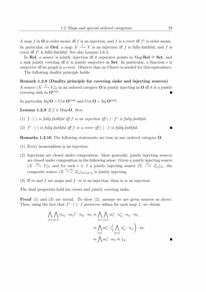
Proof (1) and (3) are trivial. To show (2), assume we are given sources as above.Then, using the fact that f ∗ · ( ) · f preserves infima for each map f , we obtain∧
i∈I
∧j∈Ji
(nij ·mi)∗ · nij ·mi ≈
∧i∈I
∧j∈Ji
m∗i · n
∗ij · nij ·mi
≈∧i∈I
m∗i ·( ∧
j∈Ji
n∗ij · nij
)·mi
≈∧
m∗i ·mi ≈ 1X
20 1 Ordered categories
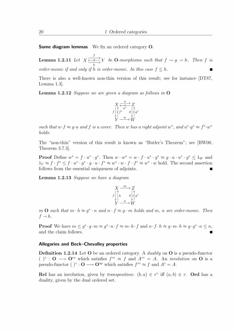
Some diagram lemmas We fix an ordered category O.
Lemma 1.2.11 Let Xf
��
h�� Yg be O-morphisms such that f −� g −� h. Then f is
order-monic if and only if h is order-monic. In this case f ≤ h.
There is also a well-known non-thin version of this result; see for instance [DT87,Lemma 1.3].
Lemma 1.2.12 Suppose we are given a diagram as follows in O
X
�f
��
⊥
u ��Z
�
u∗
g
��
Y
f∗
��
w �� W
g∗
��
such that w·f ≈ g·u and f is a cover. Then w has a right adjoint w∗, and u∗·g∗ ≈ f ∗·w∗
holds.
The “non-thin” version of this result is known as “Butler’s Theorem”; see [BW00,Theorem 3.7.3].
Proof Define w∗ = f · u∗ · g∗. Then w · w∗ = w · f · u∗ · g∗ ≈ g · u · u∗ · g∗ ≤ 1W and1Y ≈ f · f ∗ ≤ f · u∗ · g∗ · g · u · f ∗ ≈ w∗ · w · f · f ∗ ≈ w∗ · w hold. The second assertionfollows from the essential uniqueness of adjoints.
Lemma 1.2.13 Suppose we have a diagram
X
f
��
m �� Z
�g
��
Y
h
��
n �� W
g∗
��
in O such that m · h ≈ g∗ · n and n · f ≈ g ·m holds and m, n are order-monic. Thenf −� h.
Proof We have m ≤ g∗ ·g ·m ≈ g∗ ·n ·f ≈ m ·h ·f and n ·f ·h ≈ g ·m ·h ≈ g ·g∗ ·n ≤ n,and the claim follows.
Allegories and Beck–Chevalley properties
Definition 1.2.14 Let O be an ordered category. A duality on O is a pseudo-functor( )◦ : O −→ Oco which satisfies f ◦◦ ≈ f and A◦◦ = A. An involution on O is apseudo-functor ( )◦ : O −→ Oop which satisfies f ◦◦ ≈ f and A◦ = A.
Rel has an involution, given by transposition: (b, a) ∈ r◦ iff (a, b) ∈ r. Ord has aduality, given by the dual ordered set.
1.2 Maps and special ordered categories 21
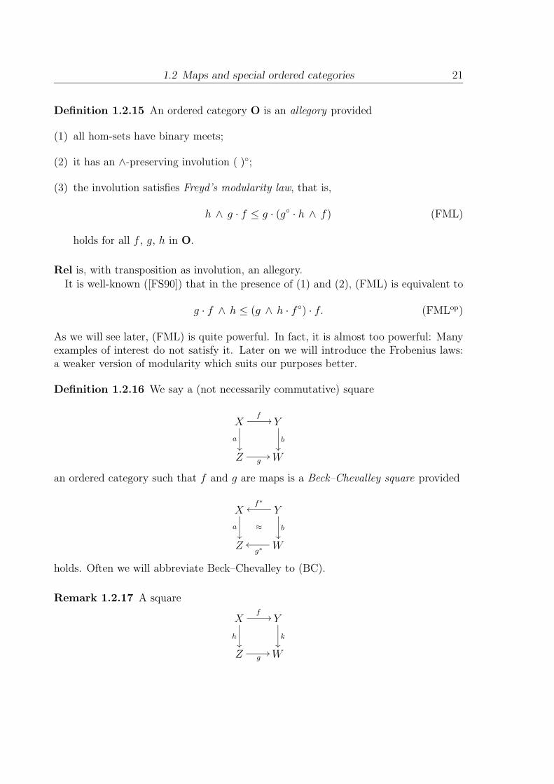
Definition 1.2.15 An ordered category O is an allegory provided
(1) all hom-sets have binary meets;
(2) it has an ∧-preserving involution ( )◦;
(3) the involution satisfies Freyd’s modularity law, that is,
h ∧ g · f ≤ g · (g◦ · h ∧ f) (FML)
holds for all f , g, h in O.
Rel is, with transposition as involution, an allegory.
It is well-known ([FS90]) that in the presence of (1) and (2), (FML) is equivalent to
g · f ∧ h ≤ (g ∧ h · f ◦) · f. (FMLop)
As we will see later, (FML) is quite powerful. In fact, it is almost too powerful: Manyexamples of interest do not satisfy it. Later on we will introduce the Frobenius laws:a weaker version of modularity which suits our purposes better.
Definition 1.2.16 We say a (not necessarily commutative) square
Xf
��
a
��
Y
b��
Z g�� W
an ordered category such that f and g are maps is a Beck–Chevalley square provided
X
a
��
≈
Yf∗
b��
Z Wg∗
holds. Often we will abbreviate Beck–Chevalley to (BC).
Remark 1.2.17 A square
Xf
��
h��
Y
k��
Z g�� W
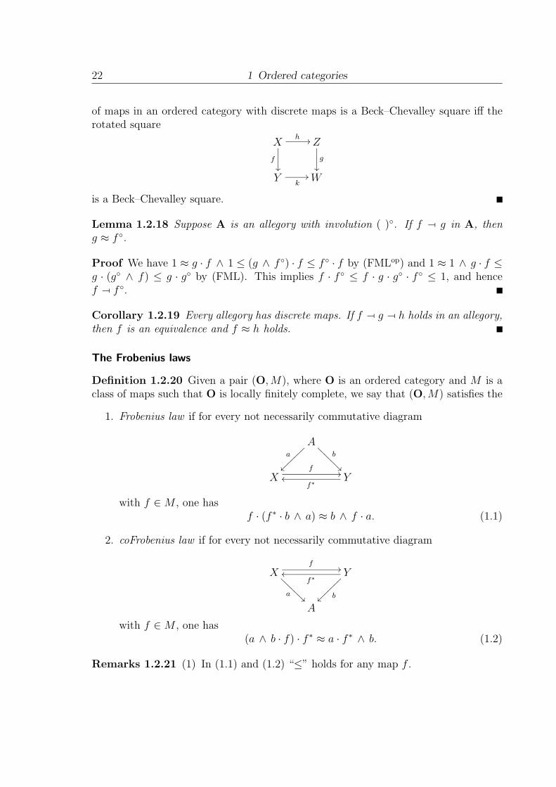
22 1 Ordered categories
of maps in an ordered category with discrete maps is a Beck–Chevalley square iff therotated square
Xh ��
f
��
Z
g
��
Yk
�� W
is a Beck–Chevalley square.
Lemma 1.2.18 Suppose A is an allegory with involution ( )◦. If f − � g in A, theng ≈ f ◦.
Proof We have 1 ≈ g · f ∧ 1 ≤ (g ∧ f ◦) · f ≤ f ◦ · f by (FMLop) and 1 ≈ 1 ∧ g · f ≤g · (g◦ ∧ f) ≤ g · g◦ by (FML). This implies f · f ◦ ≤ f · g · g◦ · f ◦ ≤ 1, and hencef −� f ◦.
Corollary 1.2.19 Every allegory has discrete maps. If f −� g −� h holds in an allegory,then f is an equivalence and f ≈ h holds.
The Frobenius laws
Definition 1.2.20 Given a pair (O,M), where O is an ordered category and M is aclass of maps such that O is locally finitely complete, we say that (O,M) satisfies the
1. Frobenius law if for every not necessarily commutative diagram
Aa
�������
b
����
����
�
Xf
��Y
f∗
with f ∈ M , one hasf · (f ∗ · b ∧ a) ≈ b ∧ f · a. (1.1)
2. coFrobenius law if for every not necessarily commutative diagram
Xf
��
a����
����
� Yf∗
b �������
A
with f ∈ M , one has(a ∧ b · f) · f ∗ ≈ a · f ∗ ∧ b. (1.2)
Remarks 1.2.21 (1) In (1.1) and (1.2) “≤” holds for any map f .

1.3 Kock–Zoberlein monads 23
(2) If O has an ∧-preserving involution ( )◦ such that f ∗ ≈ f ◦ holds for all f ∈ M ,then the Frobenius law and the coFrobenius law are equivalent.
(3) For any allegory A the Frobenius law holds in (A, MapA). In this instance, itis just (FML) (here we use Lemma 1.2.18). By (2), (A, MapA) also satisfies thecoFrobenius law.
Later on we will see examples which satisfy the Frobenius law but not (FML).
1.3 Kock–Zoberlein monads
Let O be an ordered category, T : O −→ O a pseudo-functor, and e : 1O −→ T apseudo-natural transformation. We say that (T, e) is a Kock–Zoberlein monad (KZ-monad) on O if for each X ∈ O there exists mX with
TeX −� mX −� eTX (1.3)
and mX · TeX ≈ 1TX , or equivalently, mX · eTX ≈ 1TX holds. We say that (T, e) is co-Kock–Zoberlein (coKZ) if (T, e) is Kock–Zoberlein in Oco. That is, for each O-objectX there exists mX such that
eTX − � mX −� TeX (1.4)
and mX · eTX ≈ 1TX , or equivalently, mX · TeX ≈ 1TX holds.
Proposition 1.3.1 If (T, e) is a KZ-monad on O and we are given a family (mX)such that (1.3) holds, then (T, e,m) is a pseudo-monad on O.
The distinctive feature of KZ-monads (which accounts for the title of [Koc95]) is:
Proposition 1.3.2 Let (T, e) be a KZ-monad on O. Then a pair (X,TXa−→ X) is
a (T, e,m)-pseudo-algebra iff a −� eX with a · eX ≈ 1X holds.
For a proof of the preceding results we refer to [Koc95]. Of course, dual results holdfor coKZ-monads.
Thus the existence of an (T, e)-algebra structure on an O-object O is essentially aproperty of O, and O(T,e) is essentially a (non-full) subcategory of O. Hence, KZ-monads generalize idempotent monads which correspond to reflective full and repletesubcategories.
Submonads of KZ-monads The following Proposition, which is implicit in [RW01](see also [MRW02]), is helpful in recognizing sub-KZ-monads.
24 1 Ordered categories
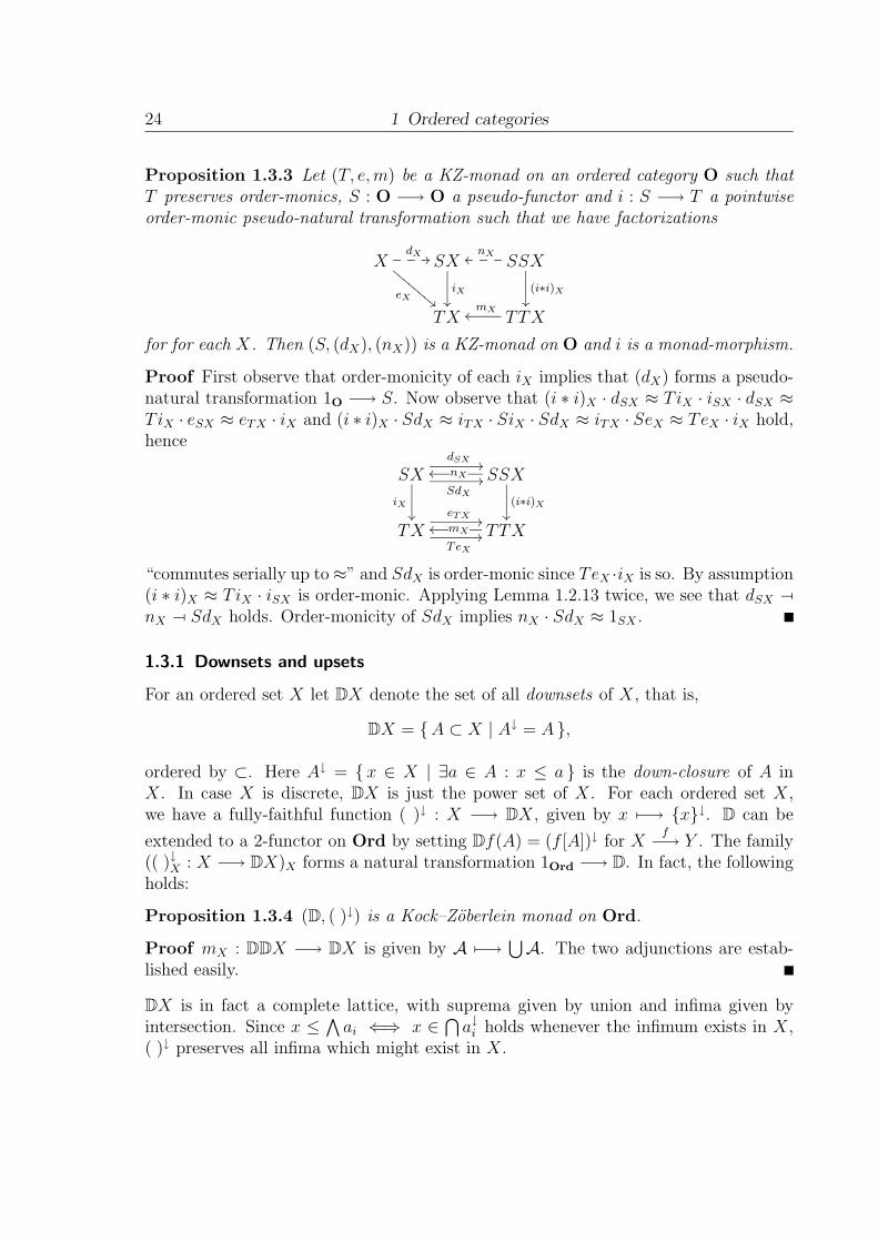
Proposition 1.3.3 Let (T, e,m) be a KZ-monad on an ordered category O such thatT preserves order-monics, S : O −→ O a pseudo-functor and i : S −→ T a pointwiseorder-monic pseudo-natural transformation such that we have factorizations
XdX �����
eX���
����
��� SX
iX��
SSXnX� � �
(i∗i)X
��
TX TTXmX
for for each X. Then (S, (dX), (nX)) is a KZ-monad on O and i is a monad-morphism.
Proof First observe that order-monicity of each iX implies that (dX) forms a pseudo-natural transformation 1O −→ S. Now observe that (i ∗ i)X · dSX ≈ TiX · iSX · dSX ≈TiX · eSX ≈ eTX · iX and (i ∗ i)X · SdX ≈ iTX · SiX · SdX ≈ iTX · SeX ≈ TeX · iX hold,hence
SX
iX��
dSX ��
SdX
�� SSXnX
(i∗i)X
��
TXeTX ��
TeX
�� TTXmX
“commutes serially up to≈” and SdX is order-monic since TeX ·iX is so. By assumption(i ∗ i)X ≈ TiX · iSX is order-monic. Applying Lemma 1.2.13 twice, we see that dSX −�
nX −� SdX holds. Order-monicity of SdX implies nX · SdX ≈ 1SX .
1.3.1 Downsets and upsets
For an ordered set X let DX denote the set of all downsets of X, that is,
DX = {A ⊂ X | A↓ = A },
ordered by ⊂. Here A↓ = {x ∈ X | ∃a ∈ A : x ≤ a } is the down-closure of A inX. In case X is discrete, DX is just the power set of X. For each ordered set X,we have a fully-faithful function ( )↓ : X −→ DX, given by x �−→ {x}↓. D can be
extended to a 2-functor on Ord by setting Df(A) = (f [A])↓ for Xf−→ Y . The family
(( )↓X : X −→ DX)X forms a natural transformation 1Ord −→ D. In fact, the followingholds:
Proposition 1.3.4 (D, ( )↓) is a Kock–Zoberlein monad on Ord.
Proof mX : DDX −→ DX is given by A �−→⋃A. The two adjunctions are estab-
lished easily.
DX is in fact a complete lattice, with suprema given by union and infima given byintersection. Since x ≤
∧ai ⇐⇒ x ∈
⋂a↓
i holds whenever the infimum exists in X,( )↓ preserves all infima which might exist in X.

1.3 Kock–Zoberlein monads 25
Remarks 1.3.5 Let f be a monotone function. The following statements hold:
(1) Df has a right adjoint D∗f , given by inverse image: D
∗f(B) = f−1[B].
(2) If f is fully-faithful, then so is Df .
An ordered set X “is” a D-algebra iff X( )↓
−→ DX has a left adjoint, that is, iff Xis complete. Moreover, a monotone function f is a D-algebra homomorphism iff fpreserves suprema. Thus OrdD is the category Sup of complete ordered sets andsuprema-preserving functions.
Dually, we define the set of upsets of an ordered set X by UX = (D(Xop))op. Thatis, UX = {A ⊂ X | A↑ = A }, with A↑ = {x ∈ X | ∃a ∈ A : a ≤ x}, ordered by ⊃.For f : X −→ Y , we have Uf(A) = (f [A])↑. Each Uf has a left adjoint U
∗f , givenby inverse image. Clearly U is a coKZ-monad on Ord. The category OrdU is just thecategory of complete ordered sets and infima-preserving functions.
1.3.2 Finitely generated downsets
We write DωX for the subset of DX given by the finitely generated downsets, that is,
DωX = {A ∈ DX | ∃B ⊂ X, B finite, A = B↓ }.
Dω is a subfunctor of D, and since finitely generated unions of finitely generateddownsets are finitely generated, Proposition 1.3.3 applies. Hence Dω is a KZ-monad onOrd, and the natural inclusion Dω −→ D forms a monad morphism.
OrdDω is the category of (finite join-) semilattices and finite join preserving mor-phisms. Dually, we obtain the finite-generated upset-monad Uω on Ord.
1.3.3 Non-empty downsets
Almost the same reasoning applies to the non-empty (or inhabited downsets) D0X ofan ordered set X, giving us a subKZ-monad D0 of D, and the corresponding subcoKZ-monad U0 of U.
1.3.4 Ideals and filters
For an ordered set X let IX = {A ∈ DX | A is directed } ⊂ DX be the set of ideals inX. Since A ⊂ X directed implies f [A] directed for all monotone functions f : X −→ Y ,and B directed implies B↓ directed, I is a subfunctor of D0. Moreover, each principaldownset x↓ is an ideal. Thus we obtain a factorization
X( )↓
��
( )↓ �����
����
� IX� �
iX��
DX

26 1 Ordered categories
where iX is fully-faithful. ( )↓ : X −→ DX preserves all infima and all finite supremawhich may exist in X. The union of any ideal of ideals is an ideal, and thus, usingProposition 1.3.3, I is a KZ-monad on Ord and i : I −→ D is a monad morphism.
Since an ordered set X is an I-algebra precisely when X( )↓
−→ IX has a left adjoint,we see that OrdI ∼= Dcpo, the category of directed complete (pre-)ordered sets anddirected suprema preserving functions; see [GHK+03].
Dually, we obtain the coKZ-monad F of filters on Ord. Here FX is given by {A ∈UX | A is filtered }. F is a sub-coKZ-monad of U.
1.3.5 Kleisli categories
Let T = (T, e,m) be a monad on C. We write CT for the Kleisli category of T, whosecomposition is, as usual, denoted by “∗”. If f : X −→ Y is any C-morphism we writef � : X −⇀ Y for the corresponding CT-morphism. We define a functor FT : C −→ CT
by X �−→ X, g �−→ (eY · g)� for g : X −→ Y .
In case T is a 2-monad on an ordered category O, OT becomes an ordered categoryin a natural way: 2-cells are inherited from O, that is, f � ≤ g� : X −⇀ Y iff f ≤ g inO. Clearly this turns FT into a 2-functor.
Distributors We define the ordered category Dist of distributors as follows: objectsare ordered sets, and morphisms X −→� Y are given by relations r ⊂ X × Y such that
x′ ≤ x, x r y, y ≤ y′ implies x′ r y′.
Composition and 2-cells are inherited from Rel. The identity on an ordered set (X,≤)is given by ≤. In contrast to Rel, Dist is not self-dual.
Remark 1.3.6 OrdopD∼= Dist ∼= Ordco
U .
Proof The isomorphisms map objects identically and transform morphisms accordingto the following scheme:
Yr−→ DX X
r−→� Y X
r−→ UY
x ∈ r(y) x r y y ∈ r(x)
For a monotone function f : X −→ Y we have xFUf y in Dist iff f(x) ≤ y in Ordand xFDf y in Dist iff y ≤ f(x) in Ord. In particular, if Y is discretely ordered thenFUf is just the graph of f and FDf is the transpose of the graph of f . But even inthe more general situation of arbitrary ordered sets, we have FUf −� FDf in Dist; seeSection 1.6.2.

1.3 Kock–Zoberlein monads 27
1.3.6 Distributive laws and composite monads
We recall that for monads T = (T, e,m) and S = (S, d, n) on a category C a distributivelaw of T over S is a natural transformation TS
r−→ ST such that
TTd
���������� dT
��
TSS
Tn��
rS �� STSSr �� SST
nT��
TSr �� ST TS
r �� ST
SeS
�� Se
����������TTS
mS
��
Tr �� TSTrT �� STT
Sm
��
(1.5)
commutes. We will use the following convention from [MRW02]: since each face of(1.5) uses precisely one of the transformations e,m, d, n, we write r[x] to indicate thata mere natural transformation TS
r−→ ST satisfies the equation from (1.5) involving
x ∈ { e,m, d, n }.For a functor G : C −→ C a distributive law of G over T is a natural transformation
GTr−→ TG which satisfies r[e] and r[m].
It is well-known that any distributive law r of T over S can be used to define a monadstructure on the composite functor ST . Indeed, the unit of the composite monad (ST)r
is given by dT · e, while the multiplication is defined by (n ∗m) · SrT .
A basic distributive law In [MRW02], the following distributive laws were described.Define natural transformations r : UD −→ DU and l : DU −→ UD as follows:
rX(A) = {U ∈ UX | ∀A ∈ A∃u ∈ U : u ∈ A },
lX(B) = {D ∈ DX | ∀B ∈ B ∃d ∈ D : d ∈ B }.
In [MRW02] it was shown that r is a distributive law of U over D and l is a distributivelaw of D over U.
Remark 1.3.7 In [MRW02] it is shown that any distributive law of T over S is unique(if it exists) provided T (or S) is either a KZ- or a coKZ-monad. Thus in this case theexistence of a distributive law is a property of the pair (S,T). In particular, l and rare the unique distributive laws of D over U and vice versa.
We are going to describe algebras for the composite monad DU = (DU)r arising fromr as above. The following discussion is due to Marmolejo, Rosebrugh, and Wood[MRW02].
Constructive complete distributivity A DU-algebra is a U-algebra which carries thestructure of a D-algebra such that the D-algebra structure-morphism is a U-morphism
28 1 Ordered categories
(this description is due to Beck [Bec69]). Thus, an ordered set X “is” a UD-algebra iffit is complete and
∨: DX −→ X is a U-morphism, that is, preserves arbitrary infima.
So we see that an ordered set X is a UD-algebra iff there exists B −�∨−� ( )↓X :
X −→ DX. These ordered sets were called constructive completely distributive (ccd)in [FW90] (see also [Woo04] and the references therein). We will contrast constructivecomplete distributivity with (classical) complete distributivity in Section 7.2.
Observe that the adjunctions D( )↓X −�⋃−� ( )↓DX for each ordered set X which verify
that (D, ( )↓) is a KZ-monad on Ord show that DX is ccd.For any ccd ordered set X, the left adjoint B : X −→ DX of
∨can be described as
follows:B(x) =
{v ∈ X
∣∣ ∀D ∈ DX : x ≤∨
D =⇒ v ∈ D}; (1.6)
see [FW90]. That is, B assigns to x all v ∈ X which are totally below x. Thus wesee the similarity between ccd ordered sets and continuous dcpos [GHK+03], which aredefined using the ideal KZ-monad I instead of D, see below.
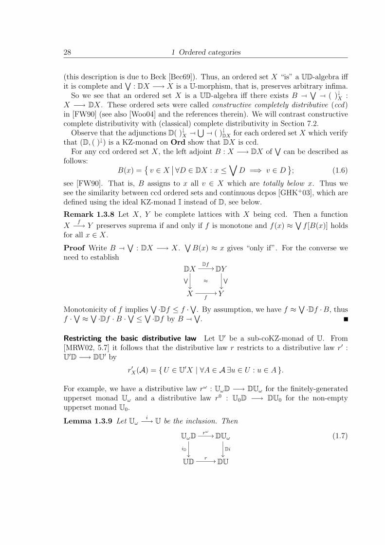
Remark 1.3.8 Let X, Y be complete lattices with X being ccd. Then a function
Xf−→ Y preserves suprema if and only if f is monotone and f(x) ≈
∨f [B(x)] holds
for all x ∈ X.
Proof Write B −�∨
: DX −→ X.∨
B(x) ≈ x gives “only if”. For the converse weneed to establish
DXDf
��
≈W
��
DYW
��
Xf
�� Y
Monotonicity of f implies∨·Df ≤ f ·
∨. By assumption, we have f ≈
∨·Df ·B, thus
f ·∨≈∨·Df ·B ·
∨≤∨·Df by B −�
∨.
Restricting the basic distributive law Let U′ be a sub-coKZ-monad of U. From
[MRW02, 5.7] it follows that the distributive law r restricts to a distributive law r′ :U
′D −→ DU
′ by
r′X(A) = {U ∈ U′X | ∀A ∈ A∃u ∈ U : u ∈ A }.
For example, we have a distributive law rω : UωD −→ DUω for the finitely-generatedupperset monad Uω and a distributive law r0 : U0D −→ DU0 for the non-emptyupperset monad U0.
Lemma 1.3.9 Let Uωi−→ U be the inclusion. Then
UωD
iD��
rω�� DUω
Di
��
UDr �� DU
(1.7)
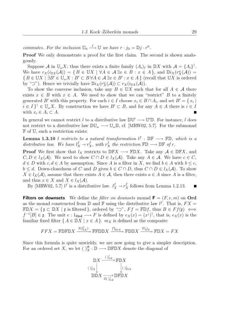
1.3 Kock–Zoberlein monads 29
commutes. For the inclusion U0j−→ U we have r · jD = Dj · r0.
Proof We only demonstrate a proof for the first claim. The second is shown analo-gously.
Suppose A in UωX; thus there exists a finite family (Ai)I in DX with A = {Ai}↑.
We have rX(iDX(A)) = {B ∈ UX | ∀A ∈ A∃x ∈ B : x ∈ A }, and DiX(rωX(A)) =
{B ∈ UX | ∃B′ ∈ UωX : B′ ⊂ B ∀A ∈ A∃x ∈ B′ : x ∈ A } (recall that UX is orderedby “⊃”). Hence we trivially have DiX(rω
X(A)) ⊂ rX(iDX(A)).To show the converse inclusion, take any B ∈ UX such that for all A ∈ A there
exists x ∈ B with x ∈ A. We need to show that we can “restrict” B to a finitelygenerated B′ with this property. For each i ∈ I choose xi ∈ B ∩Ai, and set B′ = {xi |i ∈ I }↑ ∈ UωX. By construction we have B′ ⊂ B, and for any A ∈ A there is i ∈ Iwith xi ∈ Ai ⊂ A.
In general we cannot restrict l to a distributive law DU′ −→ U
′D. For instance, l does
not restrict to a distributive law DUω −→ UωD, cf. [MRW02, 5.7]. For the submonadF of U, such a restriction exists:
Lemma 1.3.10 l restricts to a natural transformation lf : DF −→ FD, which is adistributive law. We have lfX −� rf
X , with rfX the restriction FD −→ DF of r.
Proof We first show that lX restricts to DFX −→ FDX. Take any A ∈ DFX, andC,D ∈ lX(A). We need to show C ∩ D ∈ lX(A). Take any A ∈ A. We have c ∈ C,d ∈ D with c, d ∈ A by assumption. Since A is a filter in X, we find b ∈ A with b ≤ c,b ≤ d. Down-closedness of C and D gives b ∈ C ∩D, thus C ∩D ∈ lX(A). To showX ∈ lX(A), assume that there exists A ∈ A, then there exists a ∈ A since A is a filter,and thus x ∈ X and X ∈ lX(A).
By [MRW02, 5.7] lf is a distributive law. lfX −� rfX follows from Lemma 1.2.13.
Filters on downsets We define the filter on downsets monad F = (F, e,m) on Ordas the monad constructed from D and F using the distributive law lf . That is, FX =FDX = { x ⊂ DX | x is filtered }, ordered by “⊃”, Ff = FDf , thus B ∈ Ff(x) ⇐⇒f−1[B] ∈ x. The unit e : 1Ord −→ F is defined by eX(x) = (x↓)↑, that is, eX(x) is thefamiliar fixed filter {A ∈ DX | x ∈ A }. mX is defined as the composite
FFX = FDFDXF(lf
DX)
−−−−→ FFDDXT
DDX−−−−→ FDDXF
S
X−−−→ FDX = FX
Since this formula is quite unwieldy, we are now going to give a simpler description.For an ordered set X, we let ( )#
X : D −→ DFDX denote the diagonal of
DX( )↑
DX ��
( )↓DX
��
FDX
( )↓FDX
��
DDXD( )↑
DX
�� DFDX

30 1 Ordered categories
which commutes by naturality of ( )↓. We have A# = { x ∈ FX | A ∈ x }. Observe that( )# preserves finite intersections since both ( )↑DX : DX −→ FDX and ( )↓FDX preservethem.
Lemma 1.3.11 For each ordered set X we have mX −� F( )#X .
Proof Note that we have F(lfDX) −� F(rfDX),
⋂DDX −� F( )↑DDX , and F
⋃X −� F( )↓DX
since F is a 2-functor. By uniqueness of adjoints we just have to show F( )#X =
F(rfDX) · F( )↑DDX · F( )↓DX . But we have, using the fact that rf is a distributive law,
rfDX · ( )↑DDX · ( )↓DX = D( )↑DX · ( )↓DX = ( )#
X .
Using U∗( )#
X −� U( )#X = F( )#
X and uniqueness of adjoints, we arrive at the followingdescription of mX :
A ∈ mX(X) ⇐⇒ A# ∈ X.
For a discretely ordered set X, FX is just the usual set of (possibly improper) filterson the set X. Thus we can define F : Set −→ Set as the composite
Set
F��
discrete �� Ord
F��
Set Ordforget
(1.8)
Remarks 1.3.12 (1) We have F : Ord −→ Ord as a submonad of UD, hence as asubmonad of a composite of covariant functors. For the usual filter functor on Set(as on the left side of (1.8)) no analogous result holds; it is a subfunctor of P−P−,where P− is the contravariant powerset-functor, but not of PP , cf. [MRW02, 6.4]and [Man02].
(2) For each f : X −→ Y in Ord, Ff has a right adjoint. Indeed, one has Df −� D∗f ,
and thus Ff = FDf −� F(D∗f) since F is a 2-functor. The right adjoint F ∗f of Ffsends a filter y to the filter generated by { f−1[B] | B ∈ y }.
Algebras for F Describing the (Eilenberg–Moore) algebras for F is easy: recall that,by the already used result of Beck [Bec69], specifying a F-algebra structure on anordered set X amounts to specifying a F- and a D-structure such that the F-algebrastructure-morphism is a D-homomorphism. Since an ordered set “is” a D-algebra iff ithas arbitrary suprema and a F-algebra iff it has filtered infima, we can thus characterizeFD-algebras as those complete ordered sets X that
∧: FX −→ X preserves suprema.
Equivalently,∨
: (FX)op −→ Xop preserves infima. But since (FX)op = I(Xop) bydefinition, this is equivalent to the fact that
∨: I(Xop) −→ Xop preserves infima,
that is, that Xop is a continuous lattice [GHK+03, Theorem I-1.10]. Given F-algebras
1.4 Quantaloids 31
X and Y , a monotone function f : X −→ Y is a OrdF morphism iff it preservesarbitrary suprema and filtered infima, that is, iff f : Xop −→ Y op is a homomorphismof continuous lattices.
Thus, we have exhibited OrdF as the category of “cocontinuous lattices”. Con-trast this with the well-known result of Day [Day75], who described the categories ofcontinuous lattices as SetF, where F denotes the filter-monad on Set, cf. Section 2.3.1.
1.4 Quantaloids
Definition 1.4.1 A quantaloid is an (locally small) ordered category Q such that
1. Q is locally complete;
2. composition preserves suprema in each variable.
Rel is a quantaloid. While Ord fails to be a quantaloid, its non-full subcategorySup ∼= OrdD is a quantaloid.
Since any suprema-preserving function between complete ordered sets has a rightadjoint, we obtain:
Proposition 1.4.2 Let Q be a quantaloid and Af−→ B a Q-morphism. For any
X ∈ Q both Q(f,X) and Q(X, f) have right adjoints.
We turn the last proposition into a definition:
Definition 1.4.3 We say that an ordered category O has division if for any f : A −→B in O both O(f,X) and O(X, f) have right adjoints for all X ∈ O.
1.4.1 Biproducts
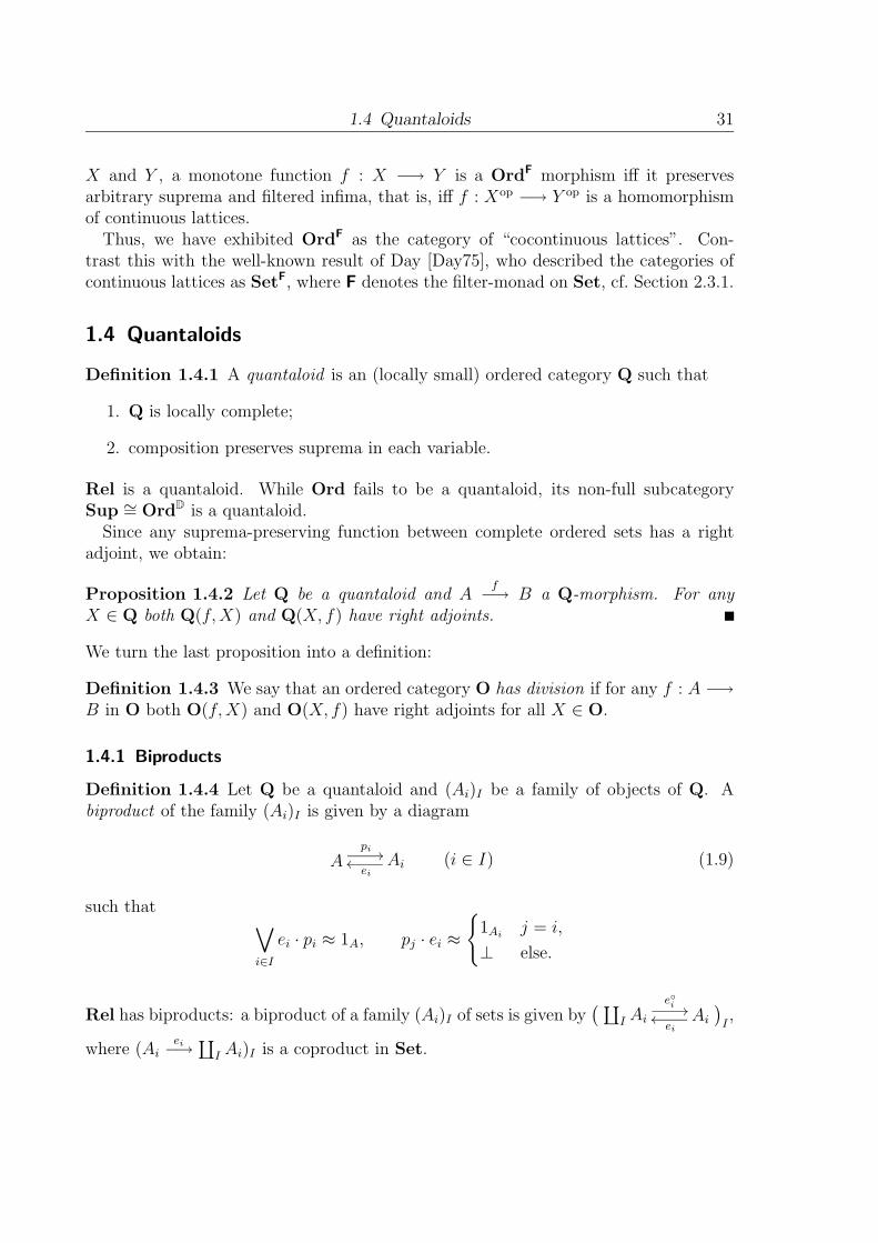
Definition 1.4.4 Let Q be a quantaloid and (Ai)I be a family of objects of Q. Abiproduct of the family (Ai)I is given by a diagram
Api ��
Aiei
(i ∈ I) (1.9)
such that ∨i∈I
ei · pi ≈ 1A, pj · ei ≈
{1Ai
j = i,
⊥ else.
Rel has biproducts: a biproduct of a family (Ai)I of sets is given by( ∐
I Ai
e◦i ��Ai
ei
)I,
where (Aiei−→∐
I Ai)I is a coproduct in Set.

32 1 Ordered categories
Of course the notion of finite biproduct can be defined in any ordered category whichis locally finitely cocomplete and in which composition preserves finite suprema; andthe following remarks are, mutatis mutandis, applicable.
The following is immediate from the definitions:
Remark 1.4.5 If (1.9) is a biproduct of the family (Ai)I , then each ei is an injectionwith right adjoint pi, and the sink (ei)I is jointly covering.
Proposition 1.4.6 If (1.9) is a biproduct of the family (Ai)I in a quantaloid, then(A, pi) is a (pseudo-)product and (A, ei) is a (pseudo-)coproduct of the family (Ai).
Proof In case of products define the morphism induced by a family (Xfi−→ Ai) by
〈fi〉 =∨
ei · fi. In case of coproducts, define the morphism induced by a family
(Aigi−→ Y ) by [gi] =
∨gi · pi.
To check that these morphisms are the unique (up the ≈) ones which make therequired diagrams commute is routine.
Proposition 1.4.7 The following statements are equivalent for a family (Ai)I of ob-jects in a quantaloid:
(1) (Ai)I has a biproduct;
(2) (Ai)I has a (pseudo-)coproduct;
(3) (Ai)I has a (pseudo-)product.
Proof By Proposition 1.4.6, (1) implies (2) and (3). To show that (2) implies (1),
suppose that (Aiei−→ A)I is a coproduct diagram. Define, for j ∈ I, pj : A −→ Aj by
pj · ei =
{1Aj
j = i,
⊥ else.
Then (A, ei, pi)i∈I is a biproduct of (Ai)I . (3) implies (1) is shown analogously.
Proposition 1.4.8 Let Q be a quantaloid and let ( Api ��
Aiei
)I be a biproduct in Q.
For a family (Aifi−→ B)I of Q-morphisms the induced morphism [fi] : A −→ B is a
map if and only if each fi is a map. Moreover, [fi] is a cover if and only if (fi) isjointly covering.
Corollary 1.4.9 If Q is a quantaloid with biproducts, then MapQ has coproducts.

1.5 Examples 33
Proof Since maps compose, each fi is a map provided f := [fi] is one.Now suppose that for each i ∈ I there exists f ∗
i with fi −� f ∗i . We claim that
∨ei ·f
∗i
is a right adjoint of f . Indeed, we have
f ·∨
ei · f∗i ≈∨
f · ei · f∗i ≈∨
fi · f∗i ≤ 1. (†)
On the other hand, f ≈∨
fi · e∗i implies
1 ≈∨
ei · e∗i ≤∨
ei · f∗i · fi · e
∗i ≤ (
∨ei · f
∗i ) · (∨
fi · e∗i ) = (
∨ei · f
∗i ) · f.
and the first claim follows. Regarding the second claim, observe that (†) is an equiva-lence provided (fi) is jointly covering. Thus f is a cover provided (fi)I covers jointly.The converse implication follows from (the dual of) Remarks 1.2.10(2).
Lemma 1.4.10 Let (Xidi−→ X)I and (Yi
ei−→ Y )I be coproducts in a quantaloid Q,
and let (Xiai−→ Yi)I be a family of Q-morphisms with induced morphism X
a−→ Y .
Then
Xidi ��
ai
��
X
a
��
Yi ei
�� Y
is a Beck–Chevalley square for each i ∈ I.
Proof Since a is the morphism induced by (ei · ai)I , we have a ≈∨
I ej · aj · d∗j , thus
e∗i · a ≈∨
e∗i · ej · aj · d∗j ≈ ai · d
∗i .
1.5 Examples
We will now discuss the notions introduced so far for two (classes of) examples.
1.5.1 Relations in regular categories
The construction of the category of relations of a given regular category is well-known.We will only list the corresponding facts here, without giving any proofs. These maybe found in the book by Freyd and Scedrov [FS90]. A category C is regular provided:
• C has finite limits;
• every kernel pair in C has a coequalizer;
• regular epimorphisms are stable under pullback in C.

34 1 Ordered categories
Every morphism f in a regular category factors as f = m · e, where m is a monomor-phism and e is a regular epimorphism. Every topos is regular, hence Set is regular.Moreover, every monadic category over Set is regular.
We will not notationally distinguish between a monomorphism and the subobject itrepresents. Given an arrow f in a regular category we write Im f for the image of f .
Let C be a well-powered regular category. The ordered category RelC of relationsin C is defined as follows:
• objects are the objects of C.
• morphisms Xr−→� Y are relations, that is, subobjects of X × Y . We write r =
〈r0, r1〉.
• 2-cells are defined according to the inclusion of subobjects.
• The identity on X is given by 〈1X , 1X〉.
• Composition is defined as follows: Given Xr−→� Y and Y
s−→� Z, we first form the
following pullback
Pq
��
p
��
S
s0
��
R r1
�� Y
and then define s · r by Im〈r0 · p, s1 · q〉.
Clearly, we have Rel (Set) ∼= Rel. RelC has an involution ( )◦, defined by transpo-sition: 〈r0, r1〉
◦ = 〈r1, r0〉. Moreover, RelC is locally finitely complete, ( )◦ commuteswith ∧, and Freyd’s modularity law holds. Hence RelC is an allegory.
We have an embedding C ↪−→ RelC which sends f : X −→ Y to its graph 〈1X , f〉,which we will also denote by f . Every graph of a C-morphism is a map, with f − � f ◦.Every map in RelC arises as the graph of a unique C-morphism, hence Map RelC ∼= C.Moreover, the graph of f is
• a cover if and only if f is a regular epimorphism, and
• an injection if and only if f is a monomorphism.
For us the most fundamental fact on RelC is:
Lemma 1.5.1 Every relation r can be written as r1 · r◦0.
Hence every morphism in RelC can be factored as the transpose of a graph of a C-morphisms followed by the graph of a C-morphism.
It is well-known that every pullback in C is a (BC)-square in RelC; see [FS90].Using this fact, we can give the following characterization of (BC)-squares in RelC:
1.5 Examples 35
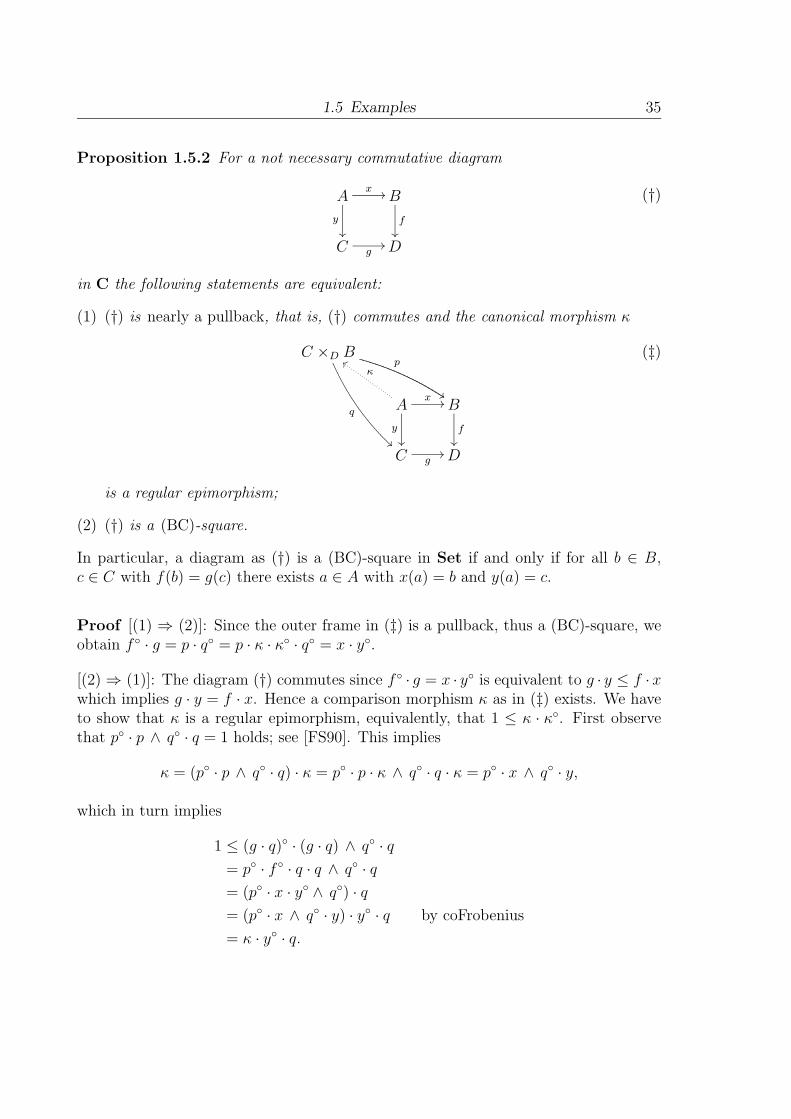
Proposition 1.5.2 For a not necessary commutative diagram
Ax ��
y
��
B
f
��
C g�� D
(†)
in C the following statements are equivalent:
(1) (†) is nearly a pullback, that is, (†) commutes and the canonical morphism κ
C ×D Bp
��
q
��
A
�
x ��
y
��
B
f
��
C g�� D
(‡)
is a regular epimorphism;
(2) (†) is a (BC)-square.
In particular, a diagram as (†) is a (BC)-square in Set if and only if for all b ∈ B,c ∈ C with f(b) = g(c) there exists a ∈ A with x(a) = b and y(a) = c.
Proof [(1) ⇒ (2)]: Since the outer frame in (‡) is a pullback, thus a (BC)-square, weobtain f◦ · g = p · q◦ = p · κ · κ◦ · q◦ = x · y◦.
[(2) ⇒ (1)]: The diagram (†) commutes since f ◦ · g = x · y◦ is equivalent to g · y ≤ f ·xwhich implies g · y = f · x. Hence a comparison morphism κ as in (‡) exists. We haveto show that κ is a regular epimorphism, equivalently, that 1 ≤ κ · κ◦. First observethat p◦ · p ∧ q◦ · q = 1 holds; see [FS90]. This implies
κ = (p◦ · p ∧ q◦ · q) · κ = p◦ · p · κ ∧ q◦ · q · κ = p◦ · x ∧ q◦ · y,
which in turn implies
1 ≤ (g · q)◦ · (g · q) ∧ q◦ · q
= p◦ · f ◦ · q · q ∧ q◦ · q
= (p◦ · x · y◦ ∧ q◦) · q
= (p◦ · x ∧ q◦ · y) · y◦ · q by coFrobenius
= κ · y◦ · q.

36 1 Ordered categories
By another application of the Frobenius law we obtain
1 ≤ p◦ · p ∧ κ · y◦ · q = κ · (κ◦ · p◦ · p ∧ y◦ · q) = κ · (x◦ · p ∧ y◦ · q) = κ · κ◦,
and the claim is proved.
More refined 2-categorical properties of RelC are summarized as follows:
(1) RelC is locally a distributive lattice, and composition distributes over finite joinsif and only if C is a prelogos (in the sense of [FS90], [Joh02] calls such a category“coherent”);
(2) RelC has division if C is a logos (in the sense of [FS90], [Joh02] calls such acategory a “Heyting category”);
(3) RelC is a quantaloid provided C has coproducts and is (infinitely) extensive.
Extending functors Suppose C and C′ are regular categories and F : C −→ C′ is anyfunctor. We are interested in the following questions: can F be extended to a 2-graphmorphism RelC −→ RelC′, and which properties does such an extension have? Thesequestions have already been considered by Carboni, Kelly, and Wood [CKW91]; seealso [Bar70], [Kam74], and [Mob81]. We state their results without proof:
Proposition 1.5.3 ([CKW91]) Define a 2-graph morphism F = Rel F : RelC −→RelC′ by
FA = FA, F (〈r0, r1〉) = Fr1 · (Fr0)◦.
Then F commutes with ( )◦ and renders
CF ��
��
C′
��
RelCF
�� RelC′
commutative. In particular, F1X = 1FX holds. Moreover,
F g · F r ≤ F (g · r) and F (r · f) ≤ F r · F f
hold for all r ∈ RelC, f, g ∈ C such that the composites are defined.F is an oplax functor if and only if F preserves regular epimorphisms, and a lax
functor if and only if F nearly preserves pullbacks, that is, for every pullback X ×Z Ythe comparison morphism F (X ×Z Y ) −→ FX ×FZ FY is a regular epimorphism.
Nearly pullback preserving functors were introduced in [JPT+01]. Occasionally, we willneed some more refined results on F defined as above; see [Kam74] and [Mob81]:

1.5 Examples 37
Proposition 1.5.4 If m ∈ MonoC, then F (m · r) = Fm · F r holds for all r ∈ RelC.If f is a C-morphism such that F preserves pullbacks along f , then F (r · f) = F r · F fholds for all r ∈ RelC.
The second condition is particularly useful when f is a monomorphism and F preservesinverse images.
Remark 1.5.5 ([CKW91]) The Rel -construction is normally oplax-functorial: given
functors CF−→ C′ G
−→ C′′ with C, C′, C′′ regular, we have Rel (1C) = 1RelC andRel (G · F ) ≤ Rel G · Rel F . Equality holds if G preserves regular epimorphisms.
Proof We write F = Rel F and G = Rel G. For a relation r = 〈r0, r1〉 in C, we have
GFr = GFr1 · (GFr0)◦ = G(Fr1) · G(Fr0)
◦ ≤ G(Fr1 · (Fr0)
◦) = GF (r)
and the inequality is an equality if G preserves regular epimorphisms.
Extending natural transformations Given functors F,G : C −→ C′ with C, C′
regular, and a natural transformation λ : F −→ G, we can consider the family Rel λ =(λX : Rel F (X) −→ Rel G(X))X of the graphs of λ. We obtain:
Proposition 1.5.6 Rel λ : Rel F −→ Rel G is an oplax transformation, that is,
FXλX ��
Rel F r
��
≤
GX
Rel G r
��
FYλY
�� GY
holds for all r = 〈r0, r1〉 ∈ RelC. Moreover, equality holds in the above diagram if theλ-naturality square of r0 is nearly a pullback.
Proof We simply calculate: λY · Rel F (r) = λY · Fr1 · (Fr0)◦ = Gr1 · λX · (Fr0)
◦ ≤Gr1 · (Gr0)
◦ ·λY = Rel G(r) ·λY . If the λ-naturality square of r0 is nearly a pullback inC, then it is a (BC)-square in RelC and equality holds.
Recall that a natural transformation λ : F −→ G is called cartesian provided
FXλX ��
Ff
��
GX
Gf
��
FYλY
�� GY
(∗)
is a pullback for all f . We call λ nearly cartesian if (∗) is nearly a pullback for all f .
Corollary 1.5.7 Rel λ is a natural transformation if and only if λ is nearly cartesian.
38 1 Ordered categories
Proof Suppose Rel λ is natural. By considering the naturality square of f ◦ = 〈f, 1Y 〉we obtain λX · Ff ◦ = Gf ◦ · λY , hence (∗) is a (BC)-square (in RelC), and thus nearlya pullback.
Instead of working with relations in a regular category, we could have studied rela-tions relative to a stable factorization system (E,M) on a finitely complete categoryX, with M ⊂ MonoX (see for instance [JW00]). Most of the results in this sectionhold in this more general setting.
1.5.2 V-Matrices
By a quantale is meant a complete lattice V equipped with a commutative, associativebinary operation ⊗, which has a unit element k and preserves suprema in each variable,that is,
u⊗∨
vi ≈∨
u⊗ vi
holds for all u, vi ∈ V (i ∈ I). Observe that our terminology differs from [Ros90] in asmuch as we always assume quantales to be commutative and unital. Hence a quantaleis a commutative monoid in the monoidal closed category Sup. Alternatively, we mayview a quantale either as
• a one-object quantaloid, or as
• a thin symmetric monoidal closed category.
In general, we write V = (V,⊗, k) to denote a quantale as above. For convenience,we will always assume V to be skeletal and non-trivial, that is, k �= ⊥.
Examples 1.5.8 (1) The most important example is the two-element chain 2 =({⊥,�},∧,�).
(2) Every frame V , in particular every complete chain and every complete Booleanalgebra, is a quantale, with ⊗ = ∧. In this case we say that V is a frame.
(3) R+ = ([0,∞]op, +, 0) where we extend + by setting a +∞ = ∞ = ∞ + a for alla ∈ [0,∞].
(4) ([0, 1],�, 1), where � is the �Lukasiewicz-conjunction, defined by
a � b = max{ 0, a + b− 1 }.
(5) Let 3 denote the 3-element chain. We equip it with the following multiplication

1.5 Examples 39
⊗ 0 1 2
0 0 0 01 0 1 22 0 2 2
This quantale is useful to construct counterexamples.
Definition 1.5.9 A quantale (V,⊗, k) is called integral if k = � holds.
Clearly the quantales in (1)–(4) above are all integral, but the one of (5) is not integral.
Remark 1.5.10 (V,⊗, k) is integral if and only if u⊗ v ≤ u∧ v holds for all u, v ∈ V .
Proof k = � implies u⊗ v ≤ u⊗ k = u and hence u⊗ v ≤ u ∧ v. On the other handwe obtain u = u⊗ k ≤ u ∧ k ≤ k for all u ∈ V , that is, k = �.
Matrices Given a quantale V = (V,⊗, k) we define the quantaloid MatV of V-matrices as follows:
• objects are sets;
• a morphism A−→� B is a function A×B −→ V ;
• the composite of Ar−→� B and B
s−→� C is given by “matrix-multiplication”
s · r(a, c) =∨b∈B
r(a, b)⊗ s(b, c) (1.10)
• the identity on A is given by the diagonal-matrix
1A(a, a′) =
{k a = a′,
⊥ else,(1.11)
where ⊥ is the bottom element of V .
The Mat-construction was introduced in [BCSW83]. The calculations to check thatMatV is indeed a quantaloid are routine. MatV has an involution ( )◦ defined byr◦(a, b) := r(b, a). In case 2 := ({0 → 1},∧, 1) we have Mat2 ∼= Rel.
Remark 1.5.11 We can recover V from MatV as V ∼= (MatV(E,E), ·, 1E), whereE is any one-element set.

40 1 Ordered categories
A universal property
Lemma 1.5.12 MatV has biproducts. In fact, it is a free biproduct-completion of V,considered as a one-object quantaloid.
Proof See [Ros01].
Denote by |V| and |MatV| the underlying category of V and MatV, respectively.Then, since Set is the coproduct-completion of the one-morphism category �, weobtain a functor
� ��
∼=��
Set ∼= Fam �
( )◦��
|V| �� |MatV|
(1.12)
where the horizontal functors are the inclusions into the respective completions and( )◦ is the unique (up to equivalence) coproduct-preserving functor such that (1.12)commutes.
We are now going to describe ( )◦: Clearly A◦ = A and
f◦(a, b) =
{k f(a) = b,
⊥ else,for f : A −→ B in Set. (1.13)
Lemma 1.5.13 Each f◦ has a right adjoint in MatV, given by (f◦)◦.
In the following we will identify a function f with its V-graph f◦. For the reader’sconvenience we note the following formulas which we will use without further reference.
For functions Xf−→ Y , Z
g−→W and V-matrices Y
a−→� Z, Z
b−→� Y we have
a · f(x, z) = a(f(x), z), f ◦ · b(z, x) = b(z, f(x)),
g · a(y, w) =∨
z∈g−1{w}
a(y, z), b · g◦(w, y) =∨
z∈g−1{w}
b(z, y).
Modularity laws We will now turn our attention to the question whether MatV isan allegory:
Lemma 1.5.14 The following statements are equivalent for an integral quantale V:
(1) ⊗ is idempotent: u⊗ u = u holds for all u ∈ V ;
(2) V is a frame: u⊗ v = u ∧ v holds for all u, v ∈ V ;
(3) MatV satisfies (FML), hence is an allegory.
Example 1.5.8(5) shows that integrality is necessary to obtain the above equivalence.

1.5 Examples 41
Proof [(1) ⇒ (2)]: By Remark 1.5.10, u⊗ v is a lower bound for {u, v}. Suppose thatz is another lower bound of {u, v}. Then z = z ⊗ z ≤ u⊗ v, and the claim follows.
[(2) ⇒ (3)]: This fact is well-known, see for example [FS90, 2.111].
[(3) ⇒ (1)]: Remark 1.5.10 gives u ⊗ u ≤ u. Specializing (FML) to matrices betweenone-element sets, with values k = � and u, we obtain u = �∧u⊗� ≤ u⊗(u⊗�∧�) =u⊗ u.
Lemma 1.5.15 The following statements are equivalent for a quantale V:
(1) V satisfies the frame law, that is, u∧∨
vi =∨
u∧ vi holds for all u, vi ∈ V , i ∈ I;
(2) (MatV,Set) satisfies the Frobenius law;
(3) (MatV,Set) satisfies the coFrobenius law.
For any V, (MatV, Mono(Set)) satisfies the Frobenius law and the coFrobenius law.
Proof ([Sch05]) Assume that V satisfies the frame law. For V-matrices Za−→� X,
Zb−→� Y , a function X
f−→ Y , and y ∈ Y , z ∈ Z, we have
f · (f ∗ · b ∧ a)(z, y) =∨
x∈f−1{y}
b(z, f(x)) ∧ a(z, x) =∨
x∈f−1{y}
b(z, y) ∧ a(z, x),
and(b ∧ f · a)(z, y) = b(z, y) ∧ (f · a(z, y)) = b(z, y) ∧
∨x∈f−1{y}
a(z, x)
which are equal by the frame law. To prove the frame law from the Frobenius law,given u ∈ V , (vi)I ⊂ V set Z = Y = {∗}, b(∗, ∗) = u, A = I, a(∗, i) = vi for all i ∈ I,and let f : I −→ {∗} be the unique function. The frame law is not needed in case f isinjective.
The equivalence of (2) and (3) follows from 1.2.21(2).
By Lemma 1.5.15, Mat R+ satisfies the Frobenius law, but by Lemma 1.5.14 it doesnot satisfy Freyd’s modular law, as was first observed in [CH03].
Maps in MatV As we have seen, every (V-graph of) a function is a map in MatV.In general, the converse implication does not hold. For example, let V be the freeBoolean algebra on one generator, so V ∼= {⊥, a,¬a,�}, with ⊗ = ∧ and k = �, andconsider the V-matrix r : 2−→� 2 given by
r =
(� a⊥ ¬a
)r is a map in MatV, but clearly r is not the V-graph of any function. In fact we havethe following result [FS90, 2.14]:

42 1 Ordered categories
Lemma 1.5.16 Suppose V is a frame. Then Map MatV ∼= Set if and only if V isconnected, that is, if v ∈ V is complemented (in the sense that there exists v′ ∈ Vsatisfying v ∧ v′ = ⊥, v ∨ v′ = �) then v = ⊥ or v = �.
Changing V Let V = (V,⊗, k) and W = (W,⊕, l) be quantales. Every functorν : V −→W induces a 2-graph morphism Mat ν : MatV −→ MatW by:
X �−→ X, r �−→ ν · r.
Proposition 1.5.17 Mat is 2-functorial: Mat 1V = 1MatV, Mat ξ ·Mat ν = Mat(ξ ·ν),and Mat ν ≤ Mat ν ′ if ν ≤ ν ′. Every Mat ν commutes with ( )◦. Moreover,
Set � �
�����
����
����
�����������
MatVMat ν �� MatW
(1.14)
commutes if and onlt if ν(⊥V ) = ⊥W and ν(k) = l hold. Any 2-graph morphism
MatVF−→ MatW which commutes with the Set-embeddings arises in this way.
Proof Functoriality of Mat is obvious; and clearly (1.14) commutes if ν(⊥V ) = ⊥W
and ν(k) = l holds. To show the converse, consider the action of Mat ν on the identityof a two-element set.
Now if F : MatV −→ MatW commutes with the embeddings of Set, then F canbe restricted to the endomorphism monoids of one-element sets in MatV and MatW,and thus gives, by Remark 1.5.11, a functor f : V −→W such that F = Mat f .
Proposition 1.5.18 Let ν : V −→W be a functor such that (1.14) commutes. Then:
(1) Mat ν(a · f) = Mat ν(a) ·Mat ν(f) holds for all V-matrices a and functions f .
(2) Mat ν(g) ·Mat ν(a) ≤ Mat ν(g · a) holds for all V-matrices a and functions g, and“=” holds if g is injective. Mat ν(g) ·Mat ν(a) = Mat ν(g · a) holds for arbitraryfunctions g and V-matrices a if and only if ν preserves suprema.
(3) Mat ν is a lax functor if and only if Vν−→W preserves ⊗ laxly, that is, νu⊗ νv ≤
ν(u⊕ v) holds.
(4) Mat ν is a 2-functor if and only if ν preserves ⊗ and suprema.
(5) Mat ν locally preserves suprema if and only if ν : V −→ W preserves suprema.

1.6 Pre-scenes 43
Embedding Rel into MatV For every quantale V we have a functor ιV : 2 −→ V,defined by ⊥ �−→ ⊥V , � �−→ kV. Clearly ιV preserves the tensor product.
Lemma 1.5.19 For any quantale V there exists a right adjoint of ιV, given by the“pessimistic” functor pV : V −→ 2, with
v �−→
{� kV ≤ v,
⊥ else.
A left adjoint of ιV exists if and only if V is integral. In this case it is given by the“optimistic” functor oV : V −→ 2, with
v �−→
{⊥ v = ⊥V ,
� else.
Both pV and oV are retractions of ιV. Moreover, the following statements hold:
• pV preserves ⊗ laxly. pV preserves ⊗ strictly if and only if kV ≤ u ⊗ v implieskV ≤ u and kV ≤ v for all u, v ∈ V .
• oV preserves ⊗ oplaxly, provided it exists. oV preserves ⊗ if and only if ⊥V is⊗-prime; that is, u⊗ v = ⊥V implies u = ⊥V or v = ⊥V for all u, v ∈ V .
Observe that the bottom element ∞ in R+ is +-prime. Thus we obtain 2-functors
Relι−→ Mat R+, Mat R+
o−→ Rel (1.15)
as well as a lax functor Relp−→ Mat R+.
1.6 Pre-scenes
A pre-scene is a diagram
S( )◦
��
( )◦�� O (1.16)
where O is an ordered category, S is a mere category, ( )◦ is a functor which is bijectiveon objects and ( )◦ : Sop −→ O is a (pseudo-)functor which satisfies f◦ −� f ◦ andS◦ = S◦ for all S-morphisms f and all S-objects S. Hence ( )◦ is determined by ( )◦ upto equivalence, its sole purpose is to provide us with a choice of right adjoints for themorphisms of S. We will just write S for S◦ or S◦. We reserve the symbol “−→” forO-morphisms of the form f◦ and denote arbitrary O-morphisms by “−→� ”. We willwrite O = (S,O) to denote a pre-scene, ( )◦ and ( )◦ will assumed to be understood.
Examples for pre-scenes are (Set, MatV), where we identify a function with its V-graph, (C, Rel C) for a regular category C, and of course (MapO,O) for any orderedcategory O.
The author may be forgiven for not studying morphisms of pre-scenes. In Chapter2, we will study morphisms of scenes, of which pre-scenes are just a special case.
44 1 Ordered categories
1.6.1 (S,O)-categories
Now we introduce O-categories for a pre-scene O = (S,O). This construction is relatedto the monad construction of Carboni, Kasangian, and Walters (restricted to a thinbicategory; see [CKW87], also [Ros96]). In case O = (Set, MatV), it amounts to theV-category construction of Lawvere (for V thin); see [Law73].
On the other hand, O-categories are a special kind of lax algebras, namely thereflexive and transitive lax algebras for the identity-monad on O. Nonetheless, we willstudy them separately in this section, concentrating on the facts which are special forthem and are not easily stated for more general lax algebras.
Definition 1.6.1 Given a pre-scene O = (S,O) we define the ordered category CatO
of O-categories and O-functors as follows:
• objects are pairs (X, a), with X an S-object and a an O-morphism X −→� Xwhich is reflexive and transitive, that is, which satisfies 1X ≤ a and a · a ≤ a;
• morphism (X, a) −→ (Y, b) are O-functors, that is, S-morphisms f : X −→ Ywhich satisfy
Xf◦
��
≤a
��
Yb��
Xf◦
�� Y
(1.17)
• for O-functors f, g : (X, a) −→ (Y, b), a 2-cell from f to g exists if and only ifg◦ ≤ b · f◦. In this case we write f ⇒ g. If f ⇒ g and g ⇒ f , we write f
∼⇒ g.
Examples
• In case O = (Set,Rel), we have Cat O ∼= Ord, as is seen easily.
• In case O = (E, Rel E) for an (elementary) topos E, we obtain the categoryOrd(E) of ordered sets in E; see [Woo04].
• Let Mon denote the regular category of monoids and monoid homomorphisms.Then C = Cat(Mon, Rel (Mon)) is the category of ordered monoids and mono-tone monoid-homomorphisms. Indeed, a C-object is given by a monoid M to-gether with a submonoid ≤ of M × M satisfying the required reflexivity andtransitivity conditions in Rel (Mon). Since pullbacks and image-factorizations inMon are concrete, we see that these are equivalent to the reflexivity and transi-tivity of the underlying relation of ≤ (on the underlying set of M). The inclusion≤↪−→M ×M is a morphism in Mon if and only if
x ≤ y, x′ ≤ y′ =⇒ xx′ ≤ yy′
1.6 Pre-scenes 45
holds. A C-morphism is a morphism of the underlying monoids which preservesthe order-relations, again by concreteness of limits and image-factorizations inMon.
• In case O = (Set, MatV), we obtain the V-categories as defined by Lawvere[Law73] (here we think of V as a thin monoidal closed category). In particular, forV = R+, we obtain the category Met of generalized metric spaces. That is, an O-category is given by a set X equipped with a distance function X×X
a−→ [0,∞].
Reflexivity of a is equivalent to a(x, x) = 0 for all x ∈ X, while transitivity of ais equivalent to the triangle inequality
a(x, z) ≤ a(x, y) + a(y, z)
for all x, y, z ∈ X. Here we use the natural order on [0,∞]. In this context (1.17)is equivalent to
∀x, x′ ∈ X : b(f(x), f(x′)) ≤ a(x, x′),
thus to f being a contraction. f ⇒ g holds if and only if we have b(f(x), g(x)) = 0for all x. Since a does not have to be symmetric, instead of thinking of a(x, x′) asthe distance of x and x′ it seems more appropriate to think of it as the amountof energy needed to transform the “system” (X, a) from state x to state x′.
If we replace R+ by any frame V, we obtain the category of V -valued ultrametricspaces.
We call a O-category (X, a) discrete if a ≈ 1X . A morphism (X, a)f−→ (Y, b) is called
fully-faithful (or initial , cartesian) if a ≈ f ◦ · b · f◦ holds. In Ord and more generallyin Ord(E), this notion of fully-faithfulness coincides with the one already used before,namely f : X −→ Y is fully-faithful if and only if
x ≤ x′ ⇐⇒ f(x) ≤ f(x′)
holds for all x, x′ ∈ X.
A characterization of adjoints in Cat O
Proposition 1.6.2 Let (X, a), (Y, b) be O-categories, and f : X −→ Y , g : Y −→ Xbe S-morphisms. The following statements are equivalent:
(1) b · f◦ ≈ g◦ · a;
(2) (X, a)f−→ (Y, b) and (Y, b)
g−→ (X, a) are O-functors and f −� g in Cat O, that is,
1X ⇒ g · f and f · g ⇒ 1Y hold.

46 1 Ordered categories
In case Cat(Set, Mat2) ∼= Ord, condition (1) translates to f(x) ≤ y ⇐⇒ x ≤ g(y)for all x ∈ X, y ∈ Y , that is, to the well-known adjointness condition for ordered sets.
Proof [(1) ⇒ (2)]: The fact that (X, a), (Y, b) are O-categories and (1) imply
1Y ≤ g◦ · g◦ ≤ g◦ · a · g◦ ≈ b · f◦ · g◦ (†)
andg◦ · f◦ ≤ g◦ · b · f◦ ≈ g◦ · g
◦ · a ≤ a. (‡)
Using (†), we obtain g◦ · b ≤ g◦ · b · b · f◦ · g◦ ≤ g◦ · b · f◦ · g◦ ≈ g◦ · g◦ · a · g◦ ≤ a · g◦ hence
(Y, b)g−→ (X, a) is a O-functor. Using (‡), we obtain f◦ · a ≤ g◦ · g◦ · f◦ · a ≤ g◦ · a · a ≤
g◦ · a ≈ b · f◦ hence also (X, a)f−→ (Y, b) is a O-functor.
Finally, (†) is equivalent to f · g ⇒ 1Y , and (‡) is equivalent to 1X ⇒ g · f .
[(2) ⇒ (1)]: We obtain, using the conditions arising from (2):
b · f◦ ≤ g◦ · g◦ · b · f◦ ≤ g◦ · a · g◦ · f◦ ≤ g◦ · a · a
≤ g◦ · a
≤ b · f◦ · g◦ · g◦ · a ≤ b · f◦ · a ≤ b · b · f◦
≤ b · f◦.
Lemma 1.6.3 Let (X, a)f
��⊥
g (Y, b) be O-functors. Then:
(1) f is fully-faithful if and only if g · f ⇒ 1X ;
(2) g is fully-faithful if and only if 1Y ⇒ f · g.
Proof Straightforward using Proposition 1.6.2.
1.6.2 (S,O)-distributors
Given O-categories (X, a) and (Y, b), a O-distributor r : (X, a)−→� (Y, b) is given byan O-morphism r : X −→� Y which satisfies
b · r ≤ r and r · a ≤ r.
We order the set of all O-distributors (X, a)−→� (Y, b) by the order induced by the oneon O(X,Y ).
Example 1.6.4 In case O = (Set,Rel), O-distributors are the same as distributorsin the sense of Section 1.3.5.

1.6 Pre-scenes 47
Lemma 1.6.5 O-distributors are closed under composition and infima in O. For everyO-category (X, a), a : (X, a)−→� (X, a) is a O-distributor which is the identity on(X, a). In case O is a quantaloid, the class of O-distributors is closed under supremain O.
Hence we have the ordered category DistO of O-categories and O-distributors. Dist O
is a quantaloid provided O is one. We remark that the construction of (S,O)-distribu-tors depends only on O. Distributors are well-known under the names ideals [CS86],monad morphisms [Ros96], compatible or ordered relations (for O = Rel, [Pis99],[HT06]), or bimodules [Law73].
We have chosen the somewhat misleading name (S,O)-distributor in view of theconnection with (S,O)-functors which we now want to make explicit:
Every O-functor f : (X, a) −→ (Y, b) gives rise to two O-distributors: we write
f∗ := b · f◦ and f ∗ := f ◦ · b. (1.18)
Lemma 1.6.6 If f : (X, a) −→ (Y, b) is a O-functor, then
(1) f∗ : (X, a)−→� (Y, b) and f ∗ : (Y, b)−→� (X, a) are O-distributors;
(2) f∗ −� f ∗ in Dist O;
(3) 1∗(X,a) = a = (1(X,a))∗ holds; and (g · f)∗ ≈ g∗ · f∗ and (g · f)∗ ≈ f ∗ · g∗ hold for anyO-functor g such that g · f is defined.
If e : (X, a) −→ (Y, b) is another O-functor, then f ⇒ e iff e∗ ≤ f∗ iff f ∗ ≤ e∗.
Corollary 1.6.7 We have pseudo-functors
Cat Oco −→ Dist O Cat Oop −→ Dist O
f �−→ f∗ f �−→ f ∗.
Both ( )∗ and ( )∗ are fully-faithful on 2-cells.
We may summarize the above results as:
Proposition 1.6.8 For every pre-scene O we obtain a pre-scene (Cat O, Dist O). Herewe consider Cat O as a mere category.
For S = Set, O = MatV, (1.18) specializes to: f∗(x, y) = b(f(x), y) and f ∗(y, x) =b(y, f(x)). For V = 2 we obtain:
x f∗ y ⇐⇒ f(x) ≤ y, y f ∗ x ⇐⇒ y ≤ f(x).
Observe that, by Proposition 1.6.2, f −� g in Cat O if and only if f∗ ≈ g∗. Therefore,every adjoint situation f −� g in Cat O gives rise to an adjoint string
g∗ − � g∗ ≈ f∗ −� f ∗ (1.19)
in Dist O.
48 1 Ordered categories
On maps in Dist O. As we have seen before, every O-functor induces an adjointsituation in Dist O. The question whether all adjoint situations are of this kind leadsto a notion of completeness for O-categories; see [Law73] and [CS86].
Lemma 1.6.9 Let f : (X, a) −→ (Y, b) be a O-functor. f∗ is an injection in Dist O ifand only if f is fully-faithful. f∗ is a cover provided f is a cover in S.
Proof f ∗ ·f∗ ≈ f ◦ ·b·b·f◦ ≈ f ◦ ·b·f◦ holds, so f ∗ ·f∗ ≈ a if and only if f is fully-faithful.In case f is a cover in S, we have f∗ · f
∗ = b · f · f ◦ · b ≈ b · b ≈ b.
A monotone function f : (X,≤) −→ (Y,≤) is a cover in Dist if and only if f “essentiallysurjective”, that is, if for every y ∈ Y there exists x ∈ X with f(x) ≈ y. To see this,observe that ≤Y⊂ f∗ · f
∗ is equivalent to ∀y, y′(y ≤ y′ =⇒ ∃x : y ≤ f(x) ≤ y′) whichis clearly equivalent to ∀y ∃x f(x) ≈ y.
Biproducts Recall that DistO is a quantaloid provided O is one.
Proposition 1.6.10 Let O be a quantaloid. If O has biproducts, so does Dist O.
Proof Given a set-indexed family (Xi, ai)I of O-categories, let(
Xpi ��
Xiei
)I
be a
biproduct in O and set a =∨
ei · ai · pi. Routine calculations show that((X, a)
ai·pi �� (Xi, ai)ei·ai
)I
is a biproduct in Dist O.
1.6.3 Duality for O-categories and O-groupoids
Definition 1.6.11 Let O = (S,O) be a pre-scene. An involution ( )t on O is said tobe compatible with O if
O( )t
��
≈
Oop
S( )◦
���������� ( )◦
��
(1.20)
holds. An involutive pre-scene is a pre-scene equipped with a compatible involution.
In this section O will be an involutive pre-scene with involution denoted by ( )◦. Thisis unambiguous by (1.20).
Definition 1.6.12 Let (X, a) be a O-category. The dual O-category (X, a)op is definedto be (X, a◦). A O-groupoid is a O-category (X, a) such that a ≈ a◦.
Proposition 1.6.13 ( )op : (X, a) �−→ (X, a)op, f �−→ f is a duality on Cat O.
We denote the full subcategory of CatO spanned by the O-groupoids by GrpdO.
1.6 Pre-scenes 49
Examples
• For O = (Set,Rel), Grpd O is the category of sets equipped with an equivalencerelation and relation-preserving functions.
• In case O = (Set, Mat R+), Grpd O is the category of symmetric generalizedmetric spaces.
More generally, if V is any quantale, Grpd(Set, MatV) is the category of globalV-valued sets and extensional functions ; see [S01, 1.2].
Proposition 1.6.14 If O locally has binary infima, then the inclusion Grpd O ↪−→Cat O has a concrete right adjoint.
Proof Given a O-category (X, a), we claim that (X, a∧a◦)1X−→ (X, a) is a couniversal
arrow. We first observe that 1X ≤ a ∧ a◦ holds, and moreover
(a ∧ a◦) · (a ∧ a◦) ≤ a · a ∧ a◦ · a ∧ a · a◦ ∧ a◦ · a◦
≤ a · a ∧ (a · a)◦
≤ a ∧ a◦,
that is, (X, a ∧ a◦) is a O-category, clearly it is also a O-groupoid. Now given any
morphism (Y, b)f−→ (X, a) in Cat O such that (Y, b) is a groupoid, we have f ·b·f ◦ ≤ a,
and thus f · b · f ◦ ≈ (f · b · f ◦)◦ ≤ a◦. Hence (Y, b)f−→ (X, a ∧ a◦) is a morphism.
1.6.4 Kleisli pre-scenes
Let T = (T, e,m) be a 2-monad on Ord such that for each f there exists Tf −� T ∗f .We define the Kleisli pre-scene KleiT
Set( )◦
��
( )◦�� OrdT
as follows: let FT, F ∗T : Ord −→ OrdT be given by FTX = F ∗
TX = X and FTf =Tf · eX = eY · f , F ∗
Tf = T ∗f · eY for f : X −→ Y in Ord. One easily checks thatFTf −� F ∗
Tf holds in OrdT. Indeed, we have FTf ∗F ∗Tf = mY ·TeY ·Tf ·T ∗f · eY ≤ eY
and eX = mX · TeX · eX ≤ mX · T (T ∗f · Tf · eX) · eX = F ∗Tf ∗ FTf . We define ( )◦ and
( )◦ as the restrictions of FT and F ∗T, respectively, to discrete ordered sets.
Given (KleiT)-categories (X, a), (Y, b) a function f : X −→ Y is a (KleiT)-functorif and only if Tf · a ≤ b · f holds in Ord.
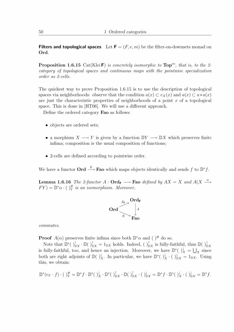
50 1 Ordered categories
Filters and topological spaces Let F = (F, e,m) be the filter-on-downsets monad onOrd.
Proposition 1.6.15 Cat(KleiF) is concretely isomorphic to Topco, that is, to the 2-category of topological spaces and continuous maps with the pointwise specializationorder as 2-cells.
The quickest way to prove Proposition 1.6.15 is to use the description of topologicalspaces via neighborhoods: observe that the condition a(x) ⊂ eX(x) and a(x) ⊂ a∗a(x)are just the characteristic properties of neighborhoods of a point x of a topologicalspace. This is done in [HT06]. We will use a different approach.
Define the ordered category Fao as follows:
• objects are ordered sets;
• a morphism X −→ Y is given by a function DY −→ DX which preserves finiteinfima; composition is the usual composition of functions;
• 2-cells are defined according to pointwise order.
We have a functor OrdE−→ Fao which maps objects identically and sends f to D
∗f .
Lemma 1.6.16 The 2-functor A : OrdF −→ Fao defined by AX = X and A(Xα−→
FY ) = D∗α · ( )#
Y is an isomorphism. Moreover,
OrdF
A
��
Ord
FF ��������
E ���������
Fao
commutes.
Proof A(α) preserves finite infima since both D∗α and ( )# do so.
Note that D∗( )↑DX · D( )↑DX = 1DX holds. Indeed, ( )↑DX is fully-faithful, thus D( )↑DX
is fully-faithful, too, and hence an injection. Moreover, we have D∗( )↓X =
⋃X since
both are right adjoints of D( )↓X . In particular, we have D∗( )↓X · ( )↓DX = 1DX . Using
this, we obtain:
D∗(eY · f) · ( )#
Y = D∗f · D∗( )↓X · D
∗( )↑DX · D( )↑DX · ( )↓DX = D∗f · D∗( )↓X · ( )↓DX = D
∗f.

1.6 Pre-scenes 51
Thus the diagram commutes and A preserves identities. To show that A preserves
composition take Xα−→ FY , Y
β−→ FZ in Ord. For C ∈ DZ and y ∈ FY , we have
y ∈ (mZ · Fβ)−1[C#] ⇐⇒ (mZ · Fβ)(y) ∈ C#
⇐⇒ C ∈ mZ(Fβ(y))
⇐⇒ C# ∈ Fβ(y)
⇐⇒ β−1[C#] ∈ y
⇐⇒ y ∈ (β−1[C#])#.
Thus, A(β ∗ α)(C) = (β ∗ α)−1[C#] = α−1[(mZ · Fβ)−1[C#]] = α−1[(β−1[C#])#] =A(β) · A(β)(C) in Fao.
Finally, define A−1 by A−1(i)(x) = {D ∈ DY | x ∈ i(D) }. The proof that A−1 is a2-functor and is inverse to A is routine.
Proof (of 1.6.15) Under the isomorphism A, a lax KleiF-category (X, a) correspondsto a set X equipped with a function i = A(a) : PX −→ PX which preserves finiteinfima. As easily seen, 1X ≤ a in OrdF is equivalent to iB ⊂ B for all B ⊂ X, whereastransitivity of a is equivalent to iB ⊂ iiB. Thus a lax algebra is equivalent to a setequipped with a topological interior operator, thus to a topological space. The proofthat a function is a KleiF-functor if and only if it is continuous is routine.
Fuzzy upsets
For an ordered set X, we can identify UX with the set of all monotone functionsX −→ 2. We will generalize this to fuzzy upsets by considering monotone functionsX −→ V, where V is an arbitrary quantale. To ease the calculations we will use thepresentation of monads as Kleisli-triples.
Kleisli-triples A Kleisli-triple on a category C is given by the following data
• a function objCT−→ objC;
• for each X ∈ objC, a morphism XeX−→ TX;
• for each X,Y ∈ objC, a function C(X,TY )( )#
−→ C(TX, TY );
subject to the following conditions
(K1) (eX)# = 1TX ;
(K2) f# · eX = f for f : X −→ TY ;
(K3) g# · f# = (g# · f)# for f : X −→ TY , g : Y −→ TZ.

52 1 Ordered categories
Every monad (T, e,m) gives rise to a Kleisli-triple (T, e, ( )#) by f# = mY ·Tf ; from aKleisli-triple we obtain a monad by Tf = (eY ·f)#, mX = 1#
TX , and these constructionsare inverse to each other; see [MS04].
In case C is an ordered category a Kleisli-triple (T, e, ( )#) on C defines a 2-monadprecisely when ( )# is monotone.
Fuzzy upsets Fix a quantale V = (V,⊗, k). We define the V-valued fuzzy upsetKleisli-triple (UV, e, ( )#) on Ord as follows:
• UVX = {Xϕ−→ V | ϕ monotone }, ordered by ϕ ≤ ψ iff ψ(x) ≤ ϕ(x) holds for
all x;
• eX : X −→ UVX by eX(x)(x′) =
{k x ≤ x′,
⊥ else;
• for f : X −→ UVY , we define f#(ϕ)(y) =∨
x∈X ϕ(x)⊗ f(x)(y).
Clearly the required monotonicity conditions are fulfilled. Ad (K1):
e#X(ϕ)(x) =
∨x′∈X
ϕ(x′)⊗ eX(x′)(x) =∨
x′≤x
ϕ(x′) = ϕ(x)
where the last equation holds since ϕ is monotone. Thus e#X = 1UVX holds. To show
(K2), observe(f# · eX(x)
)(y) = f#(eX(x))(y) =
∨x′∈X
eX(x)(x′)⊗ f(x′)(y) =∨
x≤x′
f(x′)(y) = f(x)(y);
here the last equation holds since f( )(y) is contravariantly functorial for each y ∈ Y .Finally, to show that (K3) is fulfilled, observe that(
g# · f#)(ϕ)(z) = g#(f#(ϕ))(z)
=∨y∈Y
f#(ϕ)(y)⊗ g(y)(z)
=∨y∈Y
( ∨x∈X
ϕ(x)⊗ f(x)(y)
)⊗ g(y)(z);
(†)
and (g# · f
)(ϕ)(z) =
∨x∈X
ϕ(x)⊗ (g# · f)(x)(z)
=∨x∈X
ϕ(x)⊗
( ∨y∈Y
f(x)(y)⊗ g(y)(z)
).
(‡)

1.6 Pre-scenes 53
Since ⊗ distributes over∨
, (†) and (‡) are equal. Thus, for f : X −→ Y in Ord, UVfis
UVf(ϕ)(y) = (eY · f)#(ϕ)(y) =∨x∈X
ϕ(x)⊗ eY (f(x))(y) =∨x∈X
f(x)≤y
ϕ(x).
Observe that for each f in Ord, UVf has a left adjoint U∗Vf , defined by U∗
Vf(ψ) = ψ ·f .The multiplication m is defined by mX(Φ)(x) = (1UVX)#(Φ)(x) =
∨ϕ∈UVX Φ(ϕ)⊗ϕ(x).
We remark that we did not use the commutativity of ⊗ for describing UV. In caseV = 2, UV is the upperset monad U on Ord.
Fuzzy downsets The fuzzy downsets monad DV on Ord is defined by DV(X) =(UV(Xop))op. Thus DV(X) is the set of all monotone function Xop −→ V , orderedby the pointwise order, eX : X −→ DVX is given by eX(x)(x′) = k iff x′ ≤ x and ⊥otherwise, and the extension operator ( )# for DV is defined as the one for UV. Forany f in Ord, DV(f) has a right adjoint D∗
Vf .
Fuzzy powersets We define the fuzzy-powerset monad PV for a quantale V to be the“trace” of DV to Set, that is, PV is defined as the composite
Set
PV
��
discrete�� Ord
DV
��
Set Ord,forget
where we define units and extension operators accordingly. Thus, PVX is the set V X
of all functions X −→ V .The following result can be seen as a straightforward generalization of the well-known
fact that Rel ∼= SetP = SetP2.
Remark 1.6.17 SetPVis isomorphic to the underlying category of MatV and the
isomorphism commutes with the embeddings of Set.
Proof A SetPV-morphism X
a−⇀ Y corresponds to a function X × Y
a−→ V via
a(x, y) = a(x)(y). Clearly we have eY · f = f◦. For Xa−⇀ Y
b−⇀ Z, we obtain
b ∗ a(x, z) = b#(a(x))(z) =∨y∈Y
a(x, y)⊗ b(y, z) =∨y∈Y
a(x, y)⊗ b(y, z) = b · a(x, z).

54 1 Ordered categories
2 Scenes and actors
In Section 1.6 we have defined, for any pre-scene (S,O), a notion of (S,O)-category :the objects are pairs (X, a), X a S-object and a : X −→� X an O-morphisms.
Lax algebras generalize this concept: instead of considering structures given by O-morphisms X −→� X, we consider structure-morphisms TX −→� X, where T is a specialkind of 2-graph morphism. Morphisms of lax algebras are appropriately generalized(S,O)-functors.
In fact it is convenient for the study of lax algebras to generalize from pre-scenes toscenes ; this will be done in this chapter: we introduce scenes and their morphisms.
2.1 Scenes
Definition 2.1.1 A scene S = (S,C,D) is given by the following data: a diagram
SE �� C
( )∗��
( )∗
�� D (2.1)
where
• S is a category;
• C and D are ordered categories;
• E is an embedding;
• ( )∗ is a pseudo-functor Cco −→ D, that is, ( )∗ acts covariantly on 1-cells andcontravariantly on 2-cells;
• ( )∗ is a pseudo-functor Cop −→ D, that is, ( )∗ acts contravariantly on 1-cellsand covariantly on 2-cells;
such that the following compatibility-conditions are satisfied
(1) f∗ −� f ∗ for all C-morphisms f ; in particular, C∗ = C∗ for all C-objects C;
(2) ( )∗ · E and ( )∗ · E are faithful;
(3) ( )∗ (and hence ( )∗) are bijective on objects;
(4) ( )∗ · E is locally fully-faithful, that is, f∗ ≤ g∗ implies f ≤ g (thus f = g) in S.
55

56 2 Scenes and actors
While the compatibility condition (1) is essential for all results concerning scenes, thesole purpose of (2), (3), and (4) is to ease the exposition. They are not essential.
A diagram
X
f
��
≤g
��
Y
in C is transformed into
X∗
≤
Y ∗
f∗
��
g∗
��X∗
g∗
��
≤f∗��
Y∗
We will usually not distinguish between EX and X or Ef and f . Furthermore, wewill not distinguish between C, C∗, and C∗, and often simply write f instead of f∗.As before, we will denote arbitrary D-morphisms by “−→� ”, and reserve “−→” for(( )∗-images of) S- and C-morphisms.
2.1.1 Examples
The role-model of all scenes is the distributor scene D, given by the following diagram
Setdiscrete �� Ord
( )∗��
( )∗�� Dist
where Dist = Dist(Set,Rel); and ( )∗, ( )∗ are as in (1.18); see Corollary 1.6.7.
V-matrices The scene of V-matrices for a quantale V is given by the following dia-gram
Set Set( )◦
��
( )◦�� Mat V.
Scenes whose embedding E is an isomorphism will be called discrete.
Relations For any regular category C we have a discrete scene RelC, defined by
C C( )◦
��
( )◦�� Rel C.
Distributors We write DistS for the distributor-scene of a scene S = (S,C,D), givenby
Sdiscrete �� Cat(S,D)
( )∗��
( )∗�� Dist(S,D). (2.2)

2.1 Scenes 57
Here (S,D) is the underlying pre-scene of S; see 2.2.1. If V is a quantale, we writeCatV for Cat(Set, MatV) and DistV for Dist(Set, Mat V) and obtain the scene ofV-distributors
Setdiscrete �� CatV
( )∗��
( )∗�� DistV
which is not discrete; see Corollary 1.6.7.
Ordered V-matrices For a quantale V we denote by OrdMat(V) the 1-full and 2-fullsubcategory of Dist(V) spanned by the V-categories (X, a) such that a takes values in{⊥, k}. We may identify the objects of OrdMat(V) with those of Ord. A morphism(X,≤)
r−→� (Y,≤) in OrdMat(V) is given by a V-matrix X
r−→� Y such that
x ≤ x′, y′ ≤ y implies r(x′, y′) ≤ r(x, y),
for all x, x′ ∈ X, y, y′ ∈ Y . Equivalently, r is a monotone function Xop × Y −→ V .This leads us to the following generalization of Remark 1.3.6:
Remark 2.1.2 OrdopDV
∼= OrdMat(V) ∼= OrdcoUV
.
Proof Since Ord is cartesian closed, Xop × Yr−→ V corresponds to Y
r−→ V Xop
=
DVX, thus to a morphism Xr−⇀ Y in Ordop
DV. On the other hand, r corresponds to
Xop r−→ V Y , which corresponds to X
r−→ (V Y )op = UVY .
Functoriality of these transformations is shown as in Remark 1.6.17.
For the restrictions of ( )∗ and ( )∗ to OrdMat(V) we have, in view of Remark 2.1.2,FUV
= ( )∗ : Ord −→ OrdUV
∼= OrdMat(V)co and ( )∗ = FDV: Ord −→ OrdDV
∼=OrdMat(V)op.
The scene O(V) of ordered V-matrices is defined as the following diagram
Setdiscrete �� Ord
( )∗��
( )∗�� OrdMat(V)
Clearly OrdMat(V) is, as a 1-full and 2-full subcategory of a quantaloid, a quantaloid.Moreover, it is closed under biproducts in Dist(V), hence has biproducts. For thetwo-element chain 2, O(2) = D holds.
Kleisli scenes Let T = (T, e,m) be a 2-monad on Ord such that Tf has a rightadjoint T ∗f for each f ∈ Ord. We define the Kleisli scene K(T) by
Setdiscrete �� Ord
( )∗��
( )∗�� Ordop
T
The pseudo-functor ( )∗ : Ord −→ OrdT is defined by X∗ = X and f ∗ = eY · f for anyf : X −→ Y in Ord, that is, ( )∗ is just FT. The pseudo-functor ( )∗ : Ord −→ Ordcoop
T
is defined by X∗ = X and f∗ = T ∗f · eY .

58 2 Scenes and actors
2.2 Morphisms for scenes and actors
We fix scenes S = (S,C,D) and S ′ = (S′,C′,D′).
Definition 2.2.1 A morphism of scenes (or scenic functor) S −→ S ′ is a pair (T, U)where T is a pseudo-functor C −→ C′ and U is a 2-graph morphism D −→ D′ suchthat
(M1)
C( )∗
��
T��
≈
D
U��
C′( )∗
�� D′
(2.3)
holds, that is, U(C∗) = (TC)∗ and U(f∗) ≈ (Tf)∗ hold for all C-objects C andall C-morphisms f ; so we can think of U as an “extension” of T along ( )∗.
(M2a) Uf∗ · Ua ≤ U(f∗ · a), and
(M2b) U(a · g∗) ≤ Ua · Ug∗ hold for all a ∈ D and f, g ∈ C.
An actor on S is a scenic functor S −→ S.
Examples
(1) (1C, 1D) defines a scenic functor S −→ S.
(2) Let C, C′ be regular categories and let F : C −→ C′ be an arbitrary functor. We
obtain, by Proposition 1.5.3, a scenic functor (C, Rel C)(F,Rel F )−−−−−−→ (C′, Rel C′).
(3) Suppose V = (V, k,⊗) and W = (W, l,⊕) are quantales. By Proposition 1.5.18any functor V
ν−→W which satisfies ν(k) = l and ν(⊥V ) = ν(⊥W ) defines a scenic
functor (1Set, Mat ν) : (Set, MatV) −→ (Set, MatW).
Lemma 2.2.2 Every scenic functor (T, U) as above preserves the adjointness relation:
U(f∗) − � U(f ∗)
holds for all f ∈ C.
Proof Observe first that (M1) implies U((1A)∗) ≈ (1TA)∗. Hence (M2a) implies U(f∗) ·U(f ∗) ≤ U(f∗ · f
∗) ≤ U(1∗) ≈ 1, analogously 1 ≤ U(f ∗) · U(f∗).
Preservation of the adjointness relation is in a way characteristic to scenic functorsamong certain classes of 2-graph morphisms:

2.2 Morphisms for scenes and actors 59
Lemma 2.2.3 Let T : C −→ C′ be a pseudo-functor. Given a lax or oplax functorU : D −→ D′ which extends T in the sense that (2.3) holds, (T, U) is a scenic functorif and only if U(f∗) −� U(f ∗) holds for all f ∈ C.
Proof Assume that U is lax and preserves the adjointness relation. We only need toshow (M2b): U(a · g∗) ≤ U(a · g∗) · U(g∗) · U(g∗) ≤ U(a · g∗ · g
∗) · U(g∗) ≤ Ua · U(g∗).The other assertions follow by an analogous argument.
The canonical lax extensions of [Sea05b] are lax functors which are not actors.
Lemma 2.2.4 The following statements hold for any pseudo-functor CT−→ C′ and
any 2-graph morphism DU−→ D′:
(1) If T and U fulfill (M2a) and (M2b), then (M1) is equivalent to U(C∗) = (TC)∗ andU(f ∗) ≈ (Tf)∗ for all C-objects C and all C-morphism f .
(2) The following statements are equivalent:
(i) (T, U) is a scenic functor S −→ S ′;
(ii) (M1), Ua · U(f ∗) ≤ U(a · f ∗), and U(g∗ · a) ≤ U(g∗) · Ua hold;
(iii) (M1), Uf∗ · Ua · U(g∗) ≤ U(f∗ · a · g∗), and U(f ∗ · a · g∗) ≤ U(f ∗) · Ua · Ug∗
hold.
Thus, the concept of scenic functor could be formulated in terms of ( )∗ instead of ( )∗.For a class F ⊂ morC, we write F∗ = { f∗ | f ∈ F } and F∗ = { f ∗ | f ∈ F }.
Definition 2.2.5 Given G ⊂ morD we say that (T, U) : S −→ S ′
1. is left G-strict if U(g · a) ≈ Ug · Ua holds for all g ∈ G, a ∈ D;
2. is right G-strict if U(b · g) ≈ Ub · Ug holds for all g ∈ G, b ∈ D;
3. preserves initiality if (T, U) is left (morC)∗-strict and right (morC)∗-strict, thatis, U(g∗ · a · f) ≈ U(g∗) · Ua · Uf holds for all f, g ∈ C, a ∈ D;
4. preserves finality if (T, U) is left (morC)∗-strict and right (morC)∗-strict, thatis, U(g · a · f ∗) ≈ Ug · Ua · U(f ∗) holds for all f, g ∈ C, a ∈ D.
Let F be a class of C-morphisms. We say that an actor (T, U) on S
5. preserves F-whiskers if (T, U) is left F∗-strict and right (T [F ])∗-strict;
6. preserves F∗-whiskers if (T, U) is left F∗-strict and right (T [F ])∗-strict.
Remark 2.2.6 Let (T, U) be an actor. If U is a lax functor, then (T, U) preservesinitiality. If U is an oplax functor, then (T, U) preserves finality.
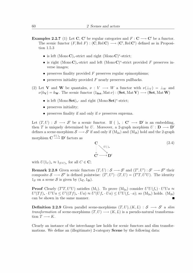
60 2 Scenes and actors
Examples 2.2.7 (1) Let C, C′ be regular categories and F : C −→ C′ be a functor.The scenic functor (F, Rel F ) : (C, RelC) −→ (C′, RelC′) defined as in Proposi-tion 1.5.3
• is left (MonoC)∗-strict and right (MonoC)∗-strict;
• is right (MonoC)∗-strict and left (MonoC)∗-strict provided F preserves in-verse images;
• preserves finality provided F preserves regular epimorphisms;
• preserves initiality provided F nearly preserves pullbacks.
(2) Let V and W be quantales, ν : V −→ W a functor with ν(⊥V ) = ⊥W andν(kV) = kW. The scenic functor (1Set, Mat ν) : (Set, MatV) −→ (Set, MatW)
• is left (MonoSet)∗- and right (MonoSet)∗-strict;
• preserves initiality;
• preserves finality if and only if ν preserves suprema.
Let (T, U) : S −→ S ′ be a scenic functor. If ( )∗ : C′ −→ D′ is an embedding,then T is uniquely determined by U . Moreover, a 2-graph morphism U : D −→ D′
defines a scene-morphism S −→ S ′ if and only if (M2a) and (M2b) hold and the 2-graph
morphism CU( )∗−→ D′ factors as
CU( )∗
��
��
C′ �� D′
(2.4)
with U(1C)∗ ≈ 1(UC)∗ for all C ∈ C;
Remark 2.2.8 Given scenic functors (T, U) : S −→ S ′ and (T ′, U ′) : S ′ −→ S ′′ theircomposite S −→ S ′′ is defined pointwise: (T ′, U ′) · (T, U) = (T ′T, U ′U). The identity1S on a scene S is given by (1C, 1D).
Proof Clearly (T ′T, U ′U) satisfies (M1). To prove (M2a) consider U ′U(f∗) · U′Ua ≈
U ′(Tf)∗ · U′Ua ≤ U ′((Tf)∗ · Ua) ≈ U ′(Uf∗ · Ua) ≤ U ′U(f∗ · a); so (M2a) holds. (M2b)
can be shown in the same manner.
Definition 2.2.9 Given parallel scene-morphisms (T, U), (K,L) : S −→ S ′ a slimtransformation of scene-morphisms (T, U) −→ (K,L) is a pseudo-natural transforma-tion T −→ K.
Clearly an instance of the interchange law holds for scenic functors and slim transfor-mations. We define an (illegitimate) 2-category Scene by the following data:

2.2 Morphisms for scenes and actors 61
• 0-cells: scenes;
• 1-cells: scenic functors;
• 2-cells: slim transformations;
with the obvious compositions.
Definition 2.2.10 We call a slim transformation (T, U)λ−→ (K,L) lax if the family(
(λC)∗)
C∈Cis a lax transformation U −→ L. Analogously for oplax and pseudo-natural
transformations.
Observe that, since the definition of scenic functor can be formulated in terms of ( )∗
instead of ( )∗, the above definition is somewhat arbitrary. In fact, we will encounterslim transformations λ : (T, U) −→ (K,L) which extend along ( )∗ (that is, the (λ∗
C :KC −→ TC) form a pseudo-natural transformation L −→ U), while λ does not extendto a pseudo-natural transformation U −→ L.
Remark 2.2.11 Let (T, T ), (S, S) : S −→ S ′ be scenic functors, λ : T −→ S a pseudo-natural transformation. (λX)∗ defines an oplax transformation T −→ S if and only ifλ∗
X defines a lax transformation S −→ T .
Definition 2.2.12 Let S = (S,C,D) and S ′ = (S′,C′,D′) be scenes. A scenic functor(F1, F2) : S −→ S ′ is based provided we have a (necessary unique) factorization
SE ��
F0
��
C
F1
��
S′E′
�� C′
Based scenic functors form a subcategory bScene ↪−→ Scene.
Actor monads In what follows we will in general not distinguish between the C andthe D part of a scene-morphism. So we will simply write U instead of (T, U), sometimeswriting UC for T .
Definition 2.2.13 An actor-monad or monadic actor is a monad structure in the2-category Scene.
To spell the above definition out, an actor-monad T = (T, e,m) on S consists of anactor T : S −→ S such that (TC, e,m) is a pseudo-monad on C.
62 2 Scenes and actors
2.2.1 Scenes vs. pre-scenes
For any pre-scene O =
(S
( )◦��
( )◦�� O
)we obtain a discrete scene SO, defined by
S S( )◦
��
( )◦�� O.
We define a morphism of pre-scenes O −→ O′ to be any scenic functor SO −→ SO′,and a transformation between such morphisms T, T ′ : O −→ O′ to be any slim trans-formation between the corresponding scenic functors SO −→ SO′. The (illegitimate)2-category PreScene of pre-scenes defined by this data is thus the 1-full and 2-fullsubcategory of Scene spanned by the SO.
Given any scene S as in (2.1), we can form its underlying pre-scene US by forgettingthe “discrete part” of S, that is, US is defined to be
C( )∗
��
( )∗�� D,
and U defines a functor U : Scene −→ PreScene.Clearly every scenic functors between pre-scenes is based. Moreover, given a scene
S as in (2.1), we can define its discretezation DS to be the pre-scene
S( )∗·E
��
( )∗·E�� D′,
where D′ is the 1-full and 2-full subcategory of D spanned by the image of ( )∗ · E.
This clearly defines a functor bSceneD−→ PreScene.
2.3 Constructing actors
We will now demonstrate various ways of constructing an actor (T, T ) from a givenfunctor T . In a way the most basic of these “extensions” is the Rel-construction,see Proposition 1.5.3, which produces an actor on (C, RelC) out of every functorT : C −→ C. A simple modification of the Rel-construction will allow us to extendfunctors from Ord to Dist. These two constructions will be the starting point for theconstruction of actors on (Set, MatV) and on O(V).
We will also present a different method using distributive laws. This has, despite itsobvious categorical appeal, “been largely overlooked” [MRW02, p. 215]. One reasonfor this omission might be that this construction gives rise to strict functors, while thefocus so far has been on lax functors. It should be worthwhile to develop — either in anorder-enriched context or for full-fledged 2-categories — a notion of “lax distributivelaw” which corresponds to lax extensions .

2.3 Constructing actors 63
Since, as we have seen in Examples 2.2.7(1), refined properties of (T, Rel T ) dependon the behavior of T with respect to pullbacks we discuss now inverse image preservingor taut1 functors; see [Mob81], [Man02].
2.3.1 Taut functors
Definition 2.3.1 ([Man02]) A functor T : C −→ C′ is taut if T sends every pullback
f−1[n]i ��
��
X
f
��
B n�� Y
(2.5)
in C with n a monomorphism to a pullback-diagram in C′. A natural transformationλ : T −→ S is taut provided the λ-naturality square
A
m
��
TA
Tm��
λA �� SA
Sm��
X TXλX
�� SX
is a pullback for all monomorphisms m. A monad (T, e,m) is taut if T , e, and m aretaut.
Every taut functor preserves monomorphisms. Weakening the concept of taut functorto “nearly taut” has no effect:
Lemma 2.3.2 Let C, C′ be categories with pullbacks. Every functor F : C −→ C′
which nearly preserves inverse images (in the sense that for any f : X −→ Y and anymonomorphism n : B −→ Y in C the canonical morphism F (f−1[n])
κ−→ FX×FY FB
is a regular epimorphism) is already taut.
Proof Let F : C −→ C′ be nearly inverse image preserving. We first show that Fpreserves monomorphisms. For any monomorphism m : A −→ X in C, we obtain acommutative diagram
FA×FX FAq
��
p
��
FA
�� � � � � �
F1A ��
F1A
��
FA
Fm��
FAFm �� FX
1This usage of the term “taut” differs from the one in, e.g., Wyler’s taut lift theorem; see [AHS04].
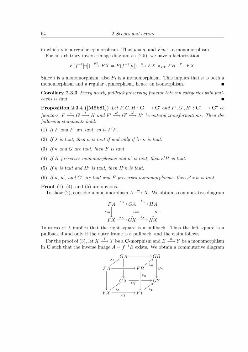
64 2 Scenes and actors
in which κ is a regular epimorphism. Thus p = q, and Fm is a monomorphism.For an arbitrary inverse image diagram as (2.5), we have a factorization
F (f−1[n])Fi−→ FX = F (f−1[n])
κ−→ FX ×FY FB
p−→ FX.
Since i is a monomorphism, also Fi is a monomorphism. This implies that κ is both amonomorphism and a regular epimorphism, hence an isomorphism.
Corollary 2.3.3 Every nearly pullback preserving functor between categories with pull-backs is taut.
Proposition 2.3.4 ([Mob81]) Let F,G,H : C −→ C′ and F ′, G′, H ′ : C′ −→ C′′ be
functors, Fκ−→ G
λ−→ H and F ′ κ′
−→ G′ λ′
−→ H ′ be natural transformations. Then thefollowing statements hold:
(1) If F and F ′ are taut, so is F ′F .
(2) If λ is taut, then κ is taut if and only if λ · κ is taut.
(3) If κ and G are taut, then F is taut.
(4) If H preserves monomorphisms and κ′ is taut, then κ′H is taut.
(5) If κ is taut and H ′ is taut, then H ′κ is taut.
(6) If κ, κ′, and G′ are taut and F preserves monomorphisms, then κ′ ∗ κ is taut.
Proof (1), (4), and (5) are obvious.To show (2), consider a monomorphism A
m−→ X. We obtain a commutative diagram
FA
Fm��
κA �� GA
Gm��
λA �� HA
Hm��
FXκX �� GX
λX �� HX
Tautness of λ implies that the right square is a pullback. Thus the left square is apullback if and only if the outer frame is a pullback, and the claim follows.
For the proof of (3), let Xf−→ Y be a C-morphism and B
n−→ Y be a monomorphism
in C such that the inverse image A = f−1B exists. We obtain a commutative diagram
GA
��
�� GB
Gn
��
FA ��
��
λA��������
FB
Fn
��
λB
������
GXGf
�� GY
FXFf
��λX
��������FY
λY
������
2.3 Constructing actors 65
In the above cube the back- and both side-faces are pullbacks. Thus also the front-faceis a pullback.
(6) follows immediately from (4), (5), and (2).
Taut functors on Set
The two trivial monads on Set are (T1, e1,m1) and (T2, e2,m2) with T1X = {∗} for allsets X and T2∅ = ∅, T2X = {∗} for X �= ∅. For justification in calling these monadstrivial see [MS04]. As is easily seen, T2 is not a taut functor, and e1 is not a tautnatural transformation: consider the naturality square of the inclusion ∅ ↪−→ X for Xnon-empty. Hence neither of the trivial monads on Set is taut, and our definition of ataut monad is coextensive with the one of [Man02].
The filter functor We write F for the filter-functor Set −→ Set; cf. (1.8). Thepowerset PX is called the nullfilter on X, every other filter is proper. We recall thatFf is defined by
Ff(x) = {B ⊂ Y | f−1B ∈ x } for Xf−→ Y.
Lemma 2.3.5 F is a taut functor.
Proof We first remark that given a subset-inclusion i : A ↪−→ X and x ∈ FX, we have
x ∈ Im Fi ⇐⇒ A ∈ x.
Hence F preserves monomorphisms, and we can consider FA as a subset of FX. To
show tautness of F , suppose we are given Wf−→ X. Assuming that all monomorphisms
are subset-inclusions, we need to show that (Ff)−1[FA] = F (f−1[A]) holds. For w ∈FW we have w ∈ (Ff)−1[FA] iff Ff(w) ∈ FA iff A ∈ Ff(w) iff f−1[A] ∈ w iffw ∈ F (f−1[A]).
Lemma 2.3.6 Every functor T : Set −→ Set which preserves binary coproducts istaut. Every natural transformation between binary coproduct preserving Set-functorsis taut.
Proof The proof shows that the lemma is valid in any extensive Boolean category; see[CLW93]:
Let Xf−→ Y be a function and B
m−→ Y be a monomorphisms. By Booleanness, we
find B′ n−→ Y such that B
m−→ Y
n←− B′ is a coproduct diagram. Forming pullbacks,
we obtainf−1[B] ��
��
X
f
��
f−1[B′]
��
Bm �� Y B′n
(†)
66 2 Scenes and actors
By extensitivity also the top row is a coproduct. Applying T to (†) we get a commu-tative diagram with top and bottom rows coproduct diagrams. By extensitivity, bothsquares in the T -image of (†) are pullbacks, and the first claim is proved.
Now given binary coproduct preserving functors T , S and a natural transformation
Tλ−→ S we obtain for B
m−→ Y as above a commutative diagram
TBTm ��
λB
��
TY
λY
��
TB′Tn
λB′
��
SBSm �� SY SB′Sn
with top and bottom rows coproducts. Thus both squares are pullbacks, and λ istaut.
Subfunctors of F We write F0X for the subset of FX consisting of the proper filters,equivalently, the x ∈ FX with ∅ /∈ x; and UX for the subset consisting of the ultrafilters,that is, maximal (with respect to ⊂) proper filters. It is well-known that a filter x onX is an ultrafilter if and only if for all A ⊂ X, either A ∈ x or X \ A ∈ x.
Lemma 2.3.7 The assignments X �−→ F0X and X �−→ UX determine subfunctorsF0 and U of F . The inclusion F0 ↪−→ F is cartesian and the inclusion U ↪−→ F istaut. In particular, both F0 and U are taut. Moreover, F0∅ = ∅ and U preserves finitecoproducts.
Proposition 2.3.8 The following statements are equivalent for a functor SetT−→ Set:
(1) T is taut;
(2) there exists a (unique) taut transformation α : T −→ F .
Moreover, α factors through the inclusion F0 ↪−→ F if and only if T preserves theinitial object, and α factors through the inclusion U ↪−→ F if and only if T preservesfinite coproducts.
The equivalence of (1) and (2) in Proposition 2.3.8 was first observed in [Mob81]; seealso [Man02].
Proof [(2) ⇒ (1)]: Tautness of α and F implies tautness of T by Proposition 2.3.4(3).
[(1) ⇒ (2)]: Let Am−→ X be a monomorphism. We wish to define α so that
TA
Tm��
αA �� FA
Fm��
TXαX �� FX
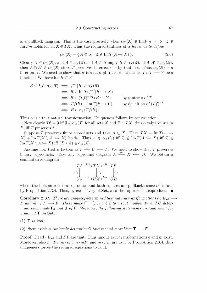
2.3 Constructing actors 67
is a pullback-diagram. This is the case precisely when αX(X) ∈ Im Fm ⇐⇒ X ∈Im Tm holds for all X ∈ TX. Thus the required tautness of α forces us to define
αX(X) = {A ⊂ X | X ∈ Im T (A ↪→ X) }. (2.6)
Clearly X ∈ αX(X); and A ∈ αX(X) and A ⊂ B imply B ∈ αX(X). If A,A′ ∈ αX(X),then A ∩ A′ ∈ αX(X) since T preserves intersections by tautness. Thus αX(X) is afilter on X. We need to show that α is a natural transformation: let f : X −→ Y be afunction. We have for B ⊂ Y :
B ∈ Ff · αX(X) ⇐⇒ f−1[B] ∈ αX(X)
⇐⇒ X ∈ Im T (f−1[B] ↪→ X)
⇐⇒ X ∈ (Tf)−1T (B ↪→ Y ) by tautness of T
⇐⇒ Tf(X) ∈ Im T (B ↪→ Y ) by definition of (Tf)−1
⇐⇒ B ∈ αY (Tf(X)).
Thus α is a taut natural transformation. Uniqueness follows by construction.Now clearly T∅ = ∅ iff ∅ /∈ αX(X) for all sets X and X ∈ TX, thus α takes values in
F0 iff T preserves ∅.Suppose T preserves finite coproducts and take A ⊂ X. Then TX = Im T (A ↪→
X) + Im T (X \ A ↪→ X) holds. Thus A /∈ αX(X) iff X /∈ Im T (A ↪→ X) iff X ∈Im T (X \ A ↪→ X) iff (X \ A) ∈ αX(X).
Assume now that α factors as Tα′
−→ U ↪−→ F . We need to show that T preservesbinary coproducts. Take any coproduct diagram A
m−→ X
n←− B. We obtain a
commutative diagram
TATm ��
α′A
��
TX
α′X
��
TB
α′B
��
Tn
UAUm �� UX UB
Un
where the bottom row is a coproduct and both squares are pullbacks since α′ is tautby Proposition 2.3.4. Thus, by extensivity of Set, also the top row is a coproduct.
Corollary 2.3.9 There are uniquely determined taut natural transformations e : 1Set −→F and m : FF −→ F . These make F = (F, e,m) into a taut monad. F0 and U deter-mine submonads F0 and U of F. Moreover, the following statements are equivalent fora monad T on Set:
(1) T is taut;
(2) there exists a (uniquely determined) taut monad-morphism T −→ F.
Proof Clearly 1Set and FF are taut. Thus unique taut transformations e and m exist.Moreover, also m ·Fe, m · eF , m ·mF , and m ·Fm are taut by Proposition 2.3.4, thusuniqueness forces the required equations to hold.

68 2 Scenes and actors
Let i : F0 ↪−→ F denote the inclusion. Since 1Set and F0F0 preserve ∅ and e as wellas m · (i ∗ i) are taut, we have factorizations
1Sete0 ��
e���
����
��� F0� �
i
��
F0F0
i∗i��
m0
F FFm
By Proposition 2.3.4, e0 and m0 are taut.
Analogously one shows that U determines a taut submonad of F.
Now if T is taut we obtain a unique transformation Tα−→ F , which is a monad-
morphism by uniqueness of taut transformations 1Set −→ F and TT −→ F . Onthe other hand, if there is a taut monad morphism T −→ F, then T is taut by thecancellation properties exhibited in Proposition 2.3.4.
The natural transformations e : 1Set −→ F and m : FF −→ F can be described easilywithout any recourse to Section 1.3.6. Using (2.6), we obtain eX(x) = {A ⊂ X | x ∈A }, thus eX(x) is just the principal filter of x. Now for X ∈ FFX we have, using (2.6)and the fact that A ∈ x if and only if x ∈ FA,
A ∈ mX(X) ⇐⇒ { x ∈ FX | A ∈ x } ∈ X.
Borger’s Lemma Proposition 2.3.8 immediately implies Borger’s Lemma [Bor87]:
Corollary 2.3.10 (Borger’s Lemma) If T : Set −→ Set preserves finite coproductsthen there is a unique natural transformation α : T −→ U .
Proof Existence follows from Proposition 2.3.8 and Lemma 2.3.6. Uniqueness followsfrom the fact that any natural transformation T −→ U is taut by Lemma 2.3.6.
Borger’s Lemma implies in particular that the monad structure on U exhibited aboveis the unique monad structure on U .
2.3.2 Constructing actors on D
Recall the distributor scene D, given by the diagram
Setdiscrete �� Ord
( )∗��
( )∗�� Dist.
We will show that every pseudo-functor Ord −→ Ord determines an actor on D.

2.3 Constructing actors 69
Factoring distributors For a distributor Xr−→� Y , we write R = { (x, y) | x r y },
ordered as a subset of X × Y . The distributor r is determined by the diagram
Xr0←− R
r1−→ Y
in Ord, here r0 and r1 are the evident projections.
Lemma 2.3.11 Every distributor Xr−→� Y factors as X
(r0)∗
−→� R(r1)∗−→� Y .
Proof Let us denote the order relation of an ordered set X by oX . Recall that r factorsin Rel as r = r1 · r
◦0. Thus, in Rel we have (r1)∗ · (r0)
∗ = oY · r1 · r◦0 · oX = oY · r · oX = r
since r is a distributor. Hence, (r1)∗ · (r0)∗ = r holds in Dist.
Extending pseudo-functors Given a pseudo-functor T : Ord −→ Ord, we can, inanalogy to the case of functors between regular categories, define an extension T :Dist −→ Dist by
TX = TX, T r = (Tr1)∗ · (Tr0)∗. (2.7)
Proposition 2.3.12 (T, T ) is an actor on D.
Proof We will first show that
Ord
T��
( )∗�� Dist
T��
Ord( )∗
�� Dist
commutes. Take any Xf−→ Y in Ord; f∗ factors as f∗ = (f1)∗ · (f0)
∗ where Xf0←−
Ff1−→ Y are the projections from F = { (x, y) | f(x) ≤ y }. Writing i : X −→ F for
the function x �−→ (x, f(x)), we obtain a diagram
Ff0
�������� f1
����
����
�
X Y
X
1X
!!��������
i
��
f
""��������
in Ord in which both triangles commute. Moreover, f ·f0 ≤ f1 holds. Thus Tf ·Tf0 ≤Tf1, which implies (Tf1)∗ ⊂ (Tf)∗ · (Tf0)∗. This gives T (f∗) = (Tf1)∗ · (Tf0)
∗ ⊂(Tf)∗ · (Tf0)∗ · (Tf0)
∗ ⊂ (Tf)∗. On the other hand, we have (Tf)∗ = (Tf1)∗ · (Ti)∗ ⊂(Tf1)∗ ·(Tf0)
∗ ·(Tf0)∗ ·(Ti)∗ = (Tf1)∗ ·(Tf0)∗ ·(T1X)∗ = T (f∗), and thus (Tf)∗ = T (f∗).
Now take any distributor Xr−→� Y and monotone functions Y
f−→ Z, W
g−→ X.
First we will show that T (f∗) · T r ⊂ T (f∗ · r) holds.

70 2 Scenes and actors
Observe that T s is actually defined for any relation s and is still locally monotoneon this larger domain. Since f ⊂ f∗ holds in Rel, it suffices to show (Tf)∗ · T r =T f∗ · T r ⊂ T (f · r).
The two “legs” of f · r are formed as follows:
C
(f ·r)0
��
(f ·r)1
��
R
d
��
�����
����� r1
����
���
Y
�����
����� f
����
���
Z
Rr1
����
���
r0
�����
YX
Hence, we have:
(Tf)∗ · T r = (Tf)∗ · (Tr1)∗ · (Tr0)∗
= (T (f · r1))∗ · (Tr0)∗
= (T (f · r)1)∗ · (Td)∗ · (Td)∗ · (T (f · r)0)∗
⊂ (T (f · r)1)∗ · (T (f · r)0)∗
= T (f · r).
To show T (r ·g∗) ⊂ T r · T (g∗), first observe that r ·g∗ = r ·g holds. Moreover, for everypullback diagram
Pq
��
p
��
R
r0
��
W g�� X
(r0, r1) being a monosource implies that also (p, r1 ·q) is a monosource. We may assumeP ⊂ W × Y , and obtain (r · g)0 = p, (r · g)1 = r1 · q. Thus
T (r · g∗) = (T (r · g)1)∗ · (T (r · g)0)∗
= (T (r1 · q))∗ · (Tp)∗
= (Tr1)∗ · (Tq)∗ · (Tp)∗
⊂ (Tr1)∗ · (Tr0)∗ · (Tg)∗
= T r · T (g∗).
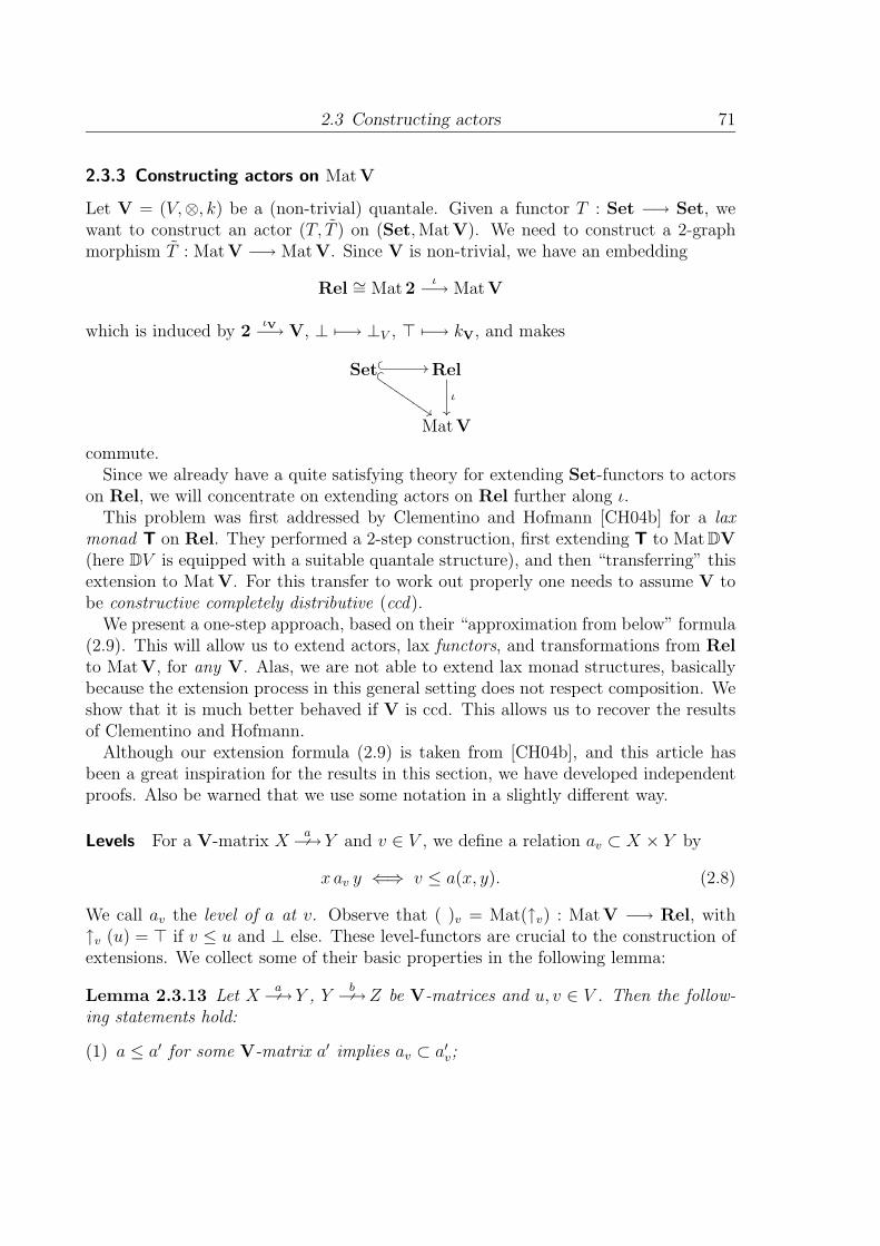
2.3 Constructing actors 71
2.3.3 Constructing actors on MatV
Let V = (V,⊗, k) be a (non-trivial) quantale. Given a functor T : Set −→ Set, wewant to construct an actor (T, T ) on (Set, MatV). We need to construct a 2-graphmorphism T : MatV −→ MatV. Since V is non-trivial, we have an embedding
Rel ∼= Mat2ι−→ MatV
which is induced by 2ιV−→ V, ⊥ �−→ ⊥V , � �−→ kV, and makes
Set� � ��� �
�����
����
��Rel
ι
��
MatV
commute.Since we already have a quite satisfying theory for extending Set-functors to actors
on Rel, we will concentrate on extending actors on Rel further along ι.This problem was first addressed by Clementino and Hofmann [CH04b] for a lax
monad T on Rel. They performed a 2-step construction, first extending T to Mat DV(here DV is equipped with a suitable quantale structure), and then “transferring” thisextension to MatV. For this transfer to work out properly one needs to assume V tobe constructive completely distributive (ccd).
We present a one-step approach, based on their “approximation from below” formula(2.9). This will allow us to extend actors, lax functors, and transformations from Relto MatV, for any V. Alas, we are not able to extend lax monad structures, basicallybecause the extension process in this general setting does not respect composition. Weshow that it is much better behaved if V is ccd. This allows us to recover the resultsof Clementino and Hofmann.
Although our extension formula (2.9) is taken from [CH04b], and this article hasbeen a great inspiration for the results in this section, we have developed independentproofs. Also be warned that we use some notation in a slightly different way.
Levels For a V-matrix Xa−→� Y and v ∈ V , we define a relation av ⊂ X × Y by
x av y ⇐⇒ v ≤ a(x, y). (2.8)
We call av the level of a at v. Observe that ( )v = Mat(↑v) : MatV −→ Rel, with↑v (u) = � if v ≤ u and ⊥ else. These level-functors are crucial to the construction ofextensions. We collect some of their basic properties in the following lemma:
Lemma 2.3.13 Let Xa−→� Y , Y
b−→� Z be V-matrices and u, v ∈ V . Then the follow-
ing statements hold:
(1) a ≤ a′ for some V-matrix a′ implies av ⊂ a′v;
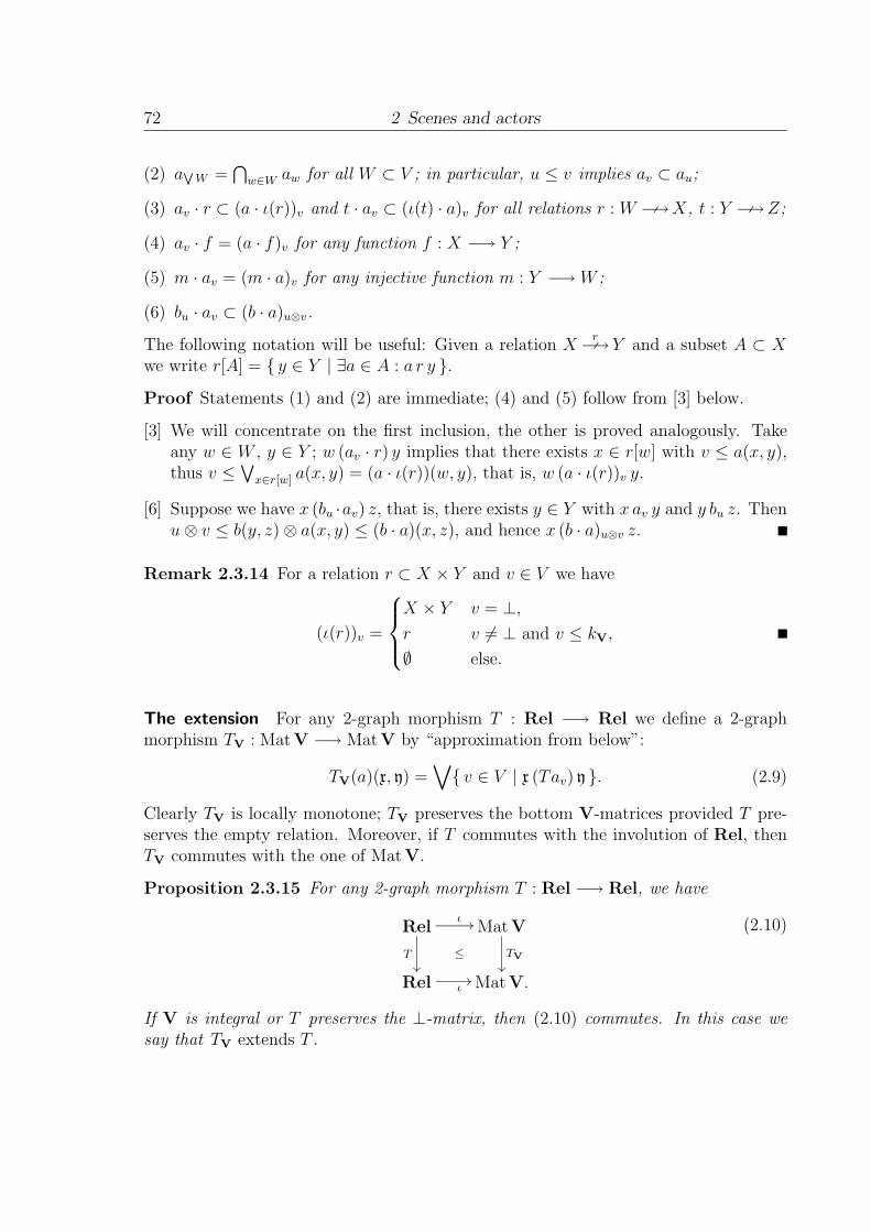
72 2 Scenes and actors
(2) aW
W =⋂
w∈W aw for all W ⊂ V ; in particular, u ≤ v implies av ⊂ au;
(3) av · r ⊂ (a · ι(r))v and t · av ⊂ (ι(t) · a)v for all relations r : W −→� X, t : Y −→� Z;
(4) av · f = (a · f)v for any function f : X −→ Y ;
(5) m · av = (m · a)v for any injective function m : Y −→W ;
(6) bu · av ⊂ (b · a)u⊗v.
The following notation will be useful: Given a relation Xr−→� Y and a subset A ⊂ X
we write r[A] = { y ∈ Y | ∃a ∈ A : a r y }.
Proof Statements (1) and (2) are immediate; (4) and (5) follow from [3] below.
[3] We will concentrate on the first inclusion, the other is proved analogously. Takeany w ∈ W , y ∈ Y ; w (av · r) y implies that there exists x ∈ r[w] with v ≤ a(x, y),thus v ≤
∨x∈r[w] a(x, y) = (a · ι(r))(w, y), that is, w (a · ι(r))v y.
[6] Suppose we have x (bu ·av) z, that is, there exists y ∈ Y with x av y and y bu z. Thenu⊗ v ≤ b(y, z)⊗ a(x, y) ≤ (b · a)(x, z), and hence x (b · a)u⊗v z.
Remark 2.3.14 For a relation r ⊂ X × Y and v ∈ V we have
(ι(r))v =
⎧⎪⎨⎪⎩X × Y v = ⊥,
r v �= ⊥ and v ≤ kV,
∅ else.
The extension For any 2-graph morphism T : Rel −→ Rel we define a 2-graphmorphism TV : MatV −→ MatV by “approximation from below”:
TV(a)(x, y) =∨{ v ∈ V | x (Tav) y }. (2.9)
Clearly TV is locally monotone; TV preserves the bottom V-matrices provided T pre-serves the empty relation. Moreover, if T commutes with the involution of Rel, thenTV commutes with the one of MatV.
Proposition 2.3.15 For any 2-graph morphism T : Rel −→ Rel, we have
Rel
T��
ι ��
≤
MatV
TV
��
Rel � MatV.
(2.10)
If V is integral or T preserves the ⊥-matrix, then (2.10) commutes. In this case wesay that TV extends T .
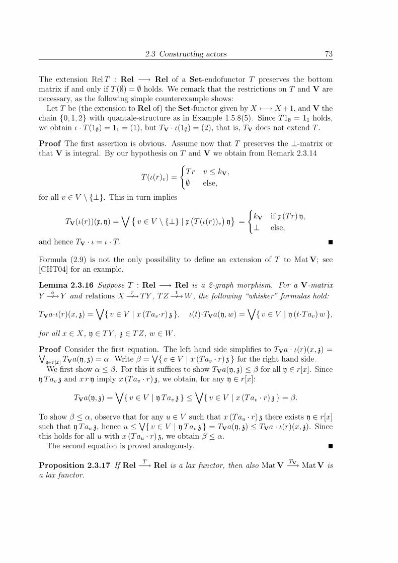
2.3 Constructing actors 73
The extension Rel T : Rel −→ Rel of a Set-endofunctor T preserves the bottommatrix if and only if T (∅) = ∅ holds. We remark that the restrictions on T and V arenecessary, as the following simple counterexample shows:
Let T be (the extension to Rel of) the Set-functor given by X �−→ X +1, and V thechain {0, 1, 2} with quantale-structure as in Example 1.5.8(5). Since T1∅ = 11 holds,we obtain ι · T (1∅) = 11 = (1), but TV · ι(1∅) = (2), that is, TV does not extend T .
Proof The first assertion is obvious. Assume now that T preserves the ⊥-matrix orthat V is integral. By our hypothesis on T and V we obtain from Remark 2.3.14
T (ι(r)v) =
{Tr v ≤ kV,
∅ else,
for all v ∈ V \ {⊥}. This in turn implies
TV(ι(r))(x, y) =∨{
v ∈ V \ {⊥} | x(T (ι(r))v
)y}
=
{kV if x (Tr) y,
⊥ else,
and hence TV · ι = ι · T .
Formula (2.9) is not the only possibility to define an extension of T to MatV; see[CHT04] for an example.
Lemma 2.3.16 Suppose T : Rel −→ Rel is a 2-graph morphism. For a V-matrix
Ya−→� Y and relations X
r−→� TY , TZ
t−→� W , the following “whisker” formulas hold:
TVa·ι(r)(x, z) =∨{ v ∈ V | x (Tav ·r) z }, ι(t)·TVa(y, w) =
∨{ v ∈ V | y (t·Tav) w },
for all x ∈ X, y ∈ TY , z ∈ TZ, w ∈ W .
Proof Consider the first equation. The left hand side simplifies to TVa · ι(r)(x, z) =∨y∈r[x] TVa(y, z) = α. Write β =
∨{ v ∈ V | x (Tav · r) z } for the right hand side.
We first show α ≤ β. For this it suffices to show TVa(y, z) ≤ β for all y ∈ r[x]. SinceyTav z and x r y imply x (Tav · r) z, we obtain, for any y ∈ r[x]:
TVa(y, z) =∨{ v ∈ V | yTav z } ≤
∨{ v ∈ V | x (Tav · r) z } = β.
To show β ≤ α, observe that for any u ∈ V such that x (Tau · r) z there exists y ∈ r[x]such that yTau z, hence u ≤
∨{ v ∈ V | y Tav z } = TVa(y, z) ≤ TVa · ι(r)(x, z). Since
this holds for all u with x (Tau · r) z, we obtain β ≤ α.The second equation is proved analogously.
Proposition 2.3.17 If RelT−→ Rel is a lax functor, then also MatV
TV−→ MatV isa lax functor.

74 2 Scenes and actors
Observe that it does not matter whether TV extends T .
Proof We have 1TVX = ι(1TX) ≤ ι(T (1X)) ≤ TVι1X = T1X for each set X.
Let Xa−→� Y
b−→� Z be V-matrices, and x ∈ TX, z ∈ TZ. We write α = TV(b ·a)(x, z).
Since TVb · TVa(x, z) =∨
y∈TY TVa(x, y)⊗ TVb(y, z), it suffices to show that
TVa(x, y)⊗ TVb(y, z) ≤ α
holds for any y ∈ TY . For each y ∈ TY we have
TVa(x, y)⊗ TVb(y, z) =
( ∨v∈V : xTav y
v
)⊗
( ∨u∈V : yTbu z
u
)=∨v∈V
xTav y
∨u∈V
yTbu z
v ⊗ u.
Thus it suffices to show u ⊗ v ≤ α whenever xTav y, y Tbu z. For each such v, u, weobtain
x (Tbu · Tav) z =⇒ x(T (bu · av)
)z since T is a lax functor
=⇒ xT (b · a)u⊗v z by Lemma 2.3.13(6).
Thus u⊗ v ≤∨{w ∈ V | xT (b · a)w z } = α.
Extending actors Let us write M for the class of V-graphs of injective functions.
Proposition 2.3.18 Let SetT−→ Set be a functor. If TV extends Rel T , then (T, TV)
is an actor on (Set, MatV). Moreover, we have the following results:
(1) (T, TV) is left M-strict and right M∗-strict;
(2) (T, TV) is right M-strict and left M∗-strict provided T is taut;
(3) TV is a lax functor provided T nearly preserves pullbacks.
Proof Let Xf−→ Y , Z
g−→ W be functions, and Y
a−→� Z be a V-matrix. (M1) holds
by assumption. To show (M2a), take any y ∈ TY , w ∈ TW ; we obtain:
TVg · TVa(y,w) = Tg · TVa(y,w)
=∨{ v ∈ V | y (Tg · Tav) w } by Lemma 2.3.16
≤∨{ v ∈ V | y T (g · av) w } since T is an actor
≤∨{ v ∈ V | y T (g · a)v w } by Lemma 2.3.13(3)
= TV(g · a)(y,w).
(2.11)

2.3 Constructing actors 75
To verify (M2b), take x ∈ TX and z ∈ TZ, then
TV(a · f)(x, z) =∨{ v ∈ V | xT (a · f)v z }
=∨{ v ∈ V | xT (av · f) z } by Lemma 2.3.13(4)
≤∨{ v ∈ V | x (Tav · Tf) z } since T is an actor
= TVa · Tf(x, z) by Lemma 2.3.16
= TVa · TVf(x, z).
(2.12)
Hence T is an actor.To show (1), assume that g is a monomorphism. Then the first inequality in (2.11) is
in fact an equality by Proposition 1.5.4 and the second inequality in (2.11) is an equalityby Lemma 2.3.13(5). The other assertion follows using the involution of MatV.
To show (2), observe that the inequality in (2.12) is, by Proposition 1.5.4, an equalityprovided T : Set −→ Set preserves pullbacks along f .
Finally, if T nearly preserves pullbacks, then Rel T is a lax functor by Proposition1.5.3, and thus TV is a lax functor by Proposition 2.3.17.
Extending natural transformations
Proposition 2.3.19 Let S, T : Rel −→ Rel be 2-graph morphisms. Every oplax (lax,natural, respectively) transformation λ : S −→ T extends to an oplax (lax, naturalrespectively) transformation SV −→ TV.
Proof We will proof the claim for oplax transformations. Suppose λ : S −→ T isoplax and let X
a−→� Y be a V-matrix. Thus we have for X ∈ SX and y ∈ TY :
λY · SV(a)(X, y) =∨{ v ∈ V | X (λY · Sav) y } by Lemma 2.3.16
≤∨{ v ∈ V | X (Tav · λX) y } since S
λ−→ T is oplax
= TVa · λX(X, y) by Lemma 2.3.16.
The proof for the case of a lax or natural transformation is now obvious.
Corollary 2.3.20 Let S, T : Set −→ Set be functors and Sλ−→ T a natural transfor-
mation. Then the V-graphs of the λX form an oplax transformation SV −→ TV, whichis a natural transformation if λ is nearly cartesian.
Proof Propositions 1.5.6 and 2.3.19.
Proposition 2.3.21 We have that (1Rel)V = 1MatV and (TS)V ≤ TVSV hold for all2-graph morphisms S, T : Rel −→ Rel; that is, the ( )V-construction is normallyoplax-functorial.

76 2 Scenes and actors
Proof Clearly (1Rel)V = 1MatV holds. To prove the second claim, observe that S(av) ⊂(SVa)v holds for all V-matrices a and all v ∈ V . Thus (TS)av ⊂ T (S(av)) ⊂ T (SVa)v
and hence (TS)V(a) ≤ TVSV(a).
Corollary 2.3.22 We have (1Set)V = 1MatV and (GF )V ≤ GVFV for all Set-functorsF,G.
Proof Remark 1.5.5 and Proposition 2.3.21.
Even though for a Set-monad (T, e,m) with T nearly pullback-preserving we obtainby the above construction a lax functor TV : MatV −→ MatV together with oplaxtransformations e : 1MatV −→ TV and m : (TT )V −→ TV, in general these data doesnot form a lax monad in the sense of [CH04b], simply because m does not need to bean oplax transformation TVTV −→ TV (since (TT )V �= TVTV).
Involving complete distributivity The preceding results can be improved if V isconstructive completely distributive (ccd); see Section 1.3.6. We do not know whetherV being ccd is necessary for the following.
Proposition 2.3.23 If V is ccd, then the ( )V-construction is preserves composition.
Proof Assume V to be ccd and let B : V −→ DV be the left adjoint of∨
. In viewof Proposition 2.3.21, it suffices to show that TVSV ≤ (TS)V holds for all 2-graphmorphisms S, T : Rel −→ Rel.
Let Xa−→� Y be a V-matrix and x ∈ TSX, y ∈ TSY . Since TVSVa(x, y) =
∨{ v ∈
V | xT (SVa)v y }, it suffices to show
v ≤ (TS)Va(x, y) =∨{w ∈W | xTS(aw) y } (†)
for all v ∈ V such that xT (SVa)v y. Fix any such v. Since the set on the right side of(†) is a downset, (†) is equivalent to
B(v) ⊂ {w ∈ V | xTS(aw) y }. (‡)
Take any u ∈ B(v). We claim that (SVa)v ⊂ S(au) holds. Indeed, for a ∈ SX, b ∈ SY ,we have
a (SVa)v b ⇐⇒ v ≤ SVa(a, b) =∨{w ∈ V | a Saw b }
where, again, the set involved is a downset. Thus, by the description (1.6) of B(v)given above, a Sau b. Since T is locally monotone, we arrive at T (SVa)v ⊂ TS(au) forall u ∈ B(v). In particular, we obtain xTS(au) y for all u ∈ B(v), and (‡) is proved.
2.3 Constructing actors 77
Proposition 2.3.24 Assume T : Rel −→ Rel to be a 2-functor and TV to extend T .If V is ccd, then
TVa · TVι(r) = TV(a · ι(r)) and TVι(s) · TVa = TV(ι(s) · a)
hold for all relations Xr−→� Y , Z
s−→� W and every V-matrix Y
a−→� Z.
Proof We will only prove the first equation. Let B : V −→ DV be the left adjoint of∨. First we shall show that for any v ∈ V , (a · ι(r))v ⊂ au · r holds for all u ∈ B(v).
Indeed, v ≤ a · ι(r)(x, z) =∨
y∈r[x] a(y, z) implies (after forming down-closures) that
there exists y ∈ r[x] with u ≤ a(y, z), that is, x (au · r) z. From this we obtainT (a · ι(r))v ⊂ T (au · r) = Tau · Tr for all u ∈ B(v). Let us write W = {w ∈ V |x (Taw · Tr)z }.
Thus xT (a · ι(r))v z implies B(v) ⊂ W ↓, equivalently, v ≤∨
W ↓ =∨
W = T a ·ι(Tr)(x, z), where the last equations holds by Lemma 2.3.16. Therefore,
TV(a · ι(r))(x, z) =∨{ v ∈ V | xT (a · ι(r))v z } ≤ TVa · ι(Tr)(x, z) = TVa · TVι(r)(x, z).
Since TV is a lax functor by Proposition 2.3.17, we are done.
Proposition 2.3.25 If V is ccd and V is a frame, then TV : MatV −→ MatV is a2-functor provided T : Rel −→ Rel is one.
Proof First observe that our hypotheses imply that TV extends T , thus preservesidentities. Let us denote the left adjoint of
∨by B. We only need to show that
TV(b · a)(x, z) ≤ TVb · TVa(x, z) holds for all Xa−→� Y
b−→� Z and x ∈ TX, z ∈ TZ.
We write W = {w ∈ V | ∃y ∈ TY : w = TVb(y, z) ∧ TVa(x, y) } and observe that itsuffices to show v ≤
∨W =
∨W ↓ for all v ∈ V such that xT (b·a)v z holds. For any such
v ∈ V and any u ∈ B(v), we claim that (b · a)v ⊂ bu · au holds. Indeed, v ≤ b · a(x, z) =∨y b(y, z)∧ a(x, y) implies that there exists y0 ∈ Y with u ≤ b(y0, z)∧ a(x, y0). This in
turn impliesT (b · a)v ⊂ T (bu · au) = Tbu · Tau.
Hence there exists y ∈ TY with xTau y and y Tbu z, thus u ≤ TVa(x, y) ∧ TVb(y, z),which implies u ∈W ↓. That is, B(v) ⊂ W ↓, and we are done.
Changing V
Proposition 2.3.26 Let V, W be quantales, Vφ−→ W a functor, and Rel
T−→ Rel
a 2-graph morphism. The following statements hold:
(1) If φ preserves suprema, then Mat φ · TV ≤ TW ·Mat φ holds.
78 2 Scenes and actors
(2) If φ preserves infima, then we have TW ·Mat φ ≤ Mat φ · TV.
The counterexample to Proposition 2.3.15 shows that (2) need not hold if φ does notpreserve infima, which for ι : 2 −→ V is equivalent to V being non-integral. In thissense the above proposition extends Proposition 2.3.15 (observe that ι : 2 −→ V alwayspreserves suprema).
Proof Let Xa−→� Y be a V-matrix.
[1] Monotonicity of φ implies av ⊂ (Mat φ(a))φ(v), and thus
Mat φ(TV(a))(x, y) = φ(∨
{ v ∈ V | xTav y })
=∨{w ∈W | ∃v ∈ V : φ(v) = w, xTav y }
≤∨{w ∈ W | ∃v ∈ V : φ(v) = w, xT (Mat φ(a))w y }
≤∨{w ∈ W | xT (Mat φ(a))w y }
= TW(Mat φ(a))(x, y)
for all x ∈ TX, y ∈ TY .
[2] Preservation of infima of φ is equivalent to the existence of χ −� φ. For each x ∈ X,y ∈ Y , we have x (Mat φ(a))w y ⇐⇒ w ≤ φ(a(x, y)) ⇐⇒ χ(w) ≤ a(x, y) ⇐⇒x aχ(w) y, and thus, for any x ∈ TX, y ∈ TY :
χ(∨
{w ∈ W | xT (aχ(w)) y })
=∨{χ(w) | w ∈ W, xT (aχ(w)) y }
≤∨{ v ∈ V | xTav y }
which implies TW(Mat φ(a))(x, y) ≤ φ(∨{v ∈ V | xTav y } = Mat φ(TV(a))(x, y).
2.3.4 From Dist to OrdMatV
We are going to use the techniques from the preceding section to extend a 2-graphmorphism on Dist = Dist(Set,Rel) = OrdMat(2) to OrdMat(V). First observe thatLemma 2.3.13(3) implies:
Corollary 2.3.27 If (X, a)r−→� (Y, b) is a morphism in OrdMat(V) and v ∈ V , then
the level rv is a distributor (X, a)−→� (Y, b).
For a 2-graph morphism DistT−→ Dist we define OrdMat(V)
TV−→ OrdMat(V) asbefore (2.9) by approximation from below:
TVr(x, y) =∨{ v ∈ V | xTrv y }. (2.13)

2.3 Constructing actors 79
We need to show that TVr is an monotone matrix whenever r is one: suppose x ≤ x′ inTX and y′ ≤ y in TY , we obtain, using that Trv is a distributor for all v ∈ V :
TVr(x′, y′) =∨{ v ∈ V | x′ Trv y′ } ≤
∨{ v ∈ V | xTrv y } = TVr(x, y).
Proposition 2.3.28 Let T : Dist −→ Dist be a 2-graph morphism and V be a quan-tale. Define TV : OrdMat(V) −→ OrdMat(V) by (2.13). Then
DistT ��
��
Dist
��
OrdMat(V)TV
�� OrdMat(V)
(2.14)
commutes provided V is integral or T preserves the bottom-distributor ∅. In this casethe following statements hold:
(1) If T is an actor on D, then TV is an actor on O(V);
(2) if T is a lax functor, so is TV;
(3) if T is a 2-functor and V is a frame with V ccd, then also TV is a 2-functor.
Proof Commutativity of (2.14) is proved as in Proposition 2.3.15.
[1] (M1) follows from the commutativity of (2.14) and the fact that T satisfies (M1).(M2a) is shown exactly as in Proposition 2.3.18. Also (M2b) is shown as in Propo-sition 2.3.18, but we have to take some care: since a · f∗ = a · f holds in Distand in OrdMat(V) for all monotone functions f and all distributors a, we obtain(a · f∗)v = (a · f)v = av · f by Lemma 2.3.13(4). Thus T (a · f∗)v = T (av · f∗) and wecan argue like in the proof of Proposition 2.3.18.
(2) and (3) follow from Proposition 2.3.17 and Proposition 2.3.25, respectively, sinceordered V-matrices are composed like (ordinary) V-matrices.
2.3.5 Extending functors to Kleisli categories
In this section we will show how to extend an endofunctor G on a category C to a functoron a Kleisli category CT. As we will see, this process is governed by a distributive lawof G over T. In fact, it is dual (in an appropriate 2-categorical sense) to the well-knownlifting of G to the Eilenberg–Moore category CT, which is governed by a distributivelaw of T over G; see [BW00]. For a proof “by duality” see, for instance, [MRW02].
Nonetheless, I decided to include an elementary proof (which I could not find inthe literature) of the correspondence between distributive laws and extensions since Ifeel that it leads to better understanding of the situation. Also, it might point the
80 2 Scenes and actors
way to an extension of the correspondence to one between “lax” extensions and “lax”distributive laws in an order-enriched context.
We shall use this technique to construct functors on Dist. Hopefully, it will alsoshed some light on the extension-process from Set to Rel.
Let T = (T, e,m) be a monad on a category C and G : C −→ C be a functor.Recall from Section 1.3.6 that a distributive law of G over T is a natural transformationGT
λ−→ TG which satisfies λ[e] and λ[m], that is, λ·Ge = eG and λ·Gm = mG·Tλ·λT
hold.
Proposition 2.3.29 There is a one-to-one correspondence between distributive lawsof G over T and extensions of G to CT, that is, functors G : CT −→ CT such that
C
G
��
FT �� CT
G��
CFT �� CT
(2.15)
commutes.
Proof Given a distributive law GTλ−→ TG of G over T, we define Gλ : CT −→ CT
by GλX = GX and
Gλ(f�) = (GX
Gf−→ GTY
λY−→ TGY )�.
First we show that Gλ · FT = FT ·G holds: given any f ∈ C, we have
Gλ(FTf) = λY ·G(Tf · eX)
= TGf · λX ·GeX
= TGf · eGX by λ[e]
= FT(Gf)
Here we omit the superscript � to increase readability. Preservation of identities isimmediate. For f : X −→ TY , g : Y −→ TZ in C, we have
λZ ·G(mZ · Tg · f) = λZ ·GmZ ·GTg ·Gf
= mGZ · TλZ · λTZ ·GTg ·Gf by λ[m]
= mGZ · TλZ · TGg · λY ·Gf
= mGZ · T (λZ ·Gg) · (λY ·Gf),
that is, Gλ(g� ∗ f �) = Gλ(g
�) ∗Gλ(f�).
Now suppose we are given a functor G : CT −→ CT such that (2.15) commutes, thatis, G(eY · f) = eGY · Gf for any f : X −→ Y in C. We define λ : GT −→ TG by

2.3 Constructing actors 81
λX = G(1�TX). We show naturality of λ: observe
TGf · λX = mGY · TeGY · TGf · λX
= mGY · T (FTGf) · G(1TX)
= G(FTf) ∗ G(1TX)
= G(FTf ∗ 1TX)
= G(Tf)
and that, since b · f = b� ∗ FTf holds for any Xf−→ Y
b−→ TZ, we have
λY ·Gh = G(1TY ) ∗ FT(Gh) = G(1TY ∗ FTh) = G(1TY · h) = G(h). (†)
for any Xh−→ TY in C. Specializing to h = Tf , we see that λ is natural. Also λ[e]
follows from (†) (with h = eX) and the fact that G preserves identities: λX ·G(eX) =G(eX) = eGX = eGX . To establish λ[m], observe that
mGX · TλX · λTX = λX ∗ λTX = G(1TX) ∗ G(1TTX) = G(1TX ∗ 1TTX) = G(mX)
holds. Thus, by (†), mGX · TλX · λTX = λX ·GmX .The proof that the constructions are mutually inverse is straightforward.
In case C is an ordered category and T , G are 2-functors, also CT is ordered, with2-cells inherited from C, and each Gλ will be a 2-functor.
Observe that we used the same ( )λ-notation as for the composite of monads formedusing λ. This should not cause any confusion, cf. Lemma 2.3.34.
Recall that, ignoring 2-categorical aspects for a moment, MatV ∼= SetPV, where PV
is the V-valued fuzzy powerset monad. In particular, Rel ∼= SetP . Thus, whenever wecan extend a functor F : Set −→ Set along the embedding to a functor MatV −→MatV, we have in fact a distributive law FPV −→ PVF .
In particular, we obtain a distributive law FP −→ PF over the powerset monad forany nearly-pullback (and regular epimorphism) preserving Set-endofunctor F . For anysuch F and any non-trivial ccd lattice V , Proposition 2.3.25 shows that the extensionF of F to MatV is a 2-functor (here V = (V,∧,�); observe that any ccd lattice is aframe, and thus V is indeed an integral quantale). Thus, Proposition 2.3.29 providesus with a distributive law FPV −→ PVF .
Functorial properties of the extension Let C be a category, T = (T, e,m) be a
monad on C, and G,H : C −→ C be functors with distributive laws GTλ−→ TG,
HTμ−→ TH over T.
Lemma 2.3.30 The identity transformation 1T : T −→ T gives a distributive law of1C over T, and ν = λH ·Gμ is a distributive law of GH over T.
82 2 Scenes and actors
Proof The first claim is obvious. Clearly ν is a natural transformation GHT −→TGH. Moreover, we have ν · GHe = λH · Gμ · GHe = λH · GeH = eGH, thus ν[e]holds. To establish ν[m], we proceed as follows:
mGH · Tν · νT = mGH · TλH · TGμ · λHT ·GμT
= mGH · TλH · λTH ·GTμ ·GμT
= λH ·GmH ·GTμ ·GμT by λ[m]
= λH ·G(mH · Tμ · μT )
= λH ·G(μ ·Hm) by μ[m]
= λH ·Gμ ·GHm
= ν ·GHm.
Proposition 2.3.31 Given functors G,H as above, we have GλHμ = (GH)ν, whereν = λH ·Gμ, and (1C)1T
= 1CT.
Proof We have (GH)ν(f) = νY · GHf = λHY · GμY · GHf = λHY · G(μY · Hf) =Gλ(Hν(f)) for any f : X −→ TY .
Proposition 2.3.32 Let Gα−→ H be a natural transformation. Then (FTαX)X is a
natural transformation Gλ −→ Hμ if and only if
GTλ ��
αT��
TG
T�
HTμ
�� TH
(2.16)
commutes. In this case we say that α extends along FT.
Proof (FTαX)X is a natural transformation precisely when FT(αY ) ∗Gλ(f) = Hμ(f) ∗FT(αX) holds for any f : X −⇀ Y in CT. In any case we have
FT(αY ) ∗Gλf = TαY ·Gλf = TαY · λY ·Gf,
and
Hμ(f) ∗ FT(αX) = μY ·Hf · αX = μY · αTY ·Gf.
Thus in case (2.16) commutes, (FTαX)X is a natural transformation. Conversely, com-mutativity of (2.16) follows from the above equations for f = 1�
TY .

2.3 Constructing actors 83
Extending monads Let S = (S, d, n) be a monad on C and μ : ST −→ TS adistributive law of S over T. Then d and n extend to natural transformations 1CT
−→Sμ and SμSμ −→ Sμ precisely when d and n satisfy the extension condition (2.16) forλ = 1T and λ = μS · Sμ, respectively. But this is the case precisely when μ satisfiesμ[n] and μ[d], that is, if and only if μ is a distributive law of S over T in the sense ofSection 1.3.6. Thus we have shown:
Proposition 2.3.33 There is a one-to-one correspondence between distributive laws μof S over T and extensions of S to CT.
We recall that μ as above allows us to construct a monad structure on the compositefunctor TS, and that this monad is denoted by (TS)μ.
Lemma 2.3.34 There is an isomorphism H : C(TS)μ−→ (CT)Sμ
which makes
CFT ��
F(TS)μ
��
CT
FSμ
��
C(TS)μ
H �� (CT)Sμ
(2.17)
commute.
An example We will now try to illustrate the results of this section with the exampleof the upper-set monad U on Ord. Using the distributive law UD
r−→ DU we obtain a
2-monad (Ur, ( )↑,⋃
) on OrdD∼= Distop. We can consider Ur as a 2-functor Dist −→
Dist which makes
Ord
U
��
( )∗�� Dist
Ur
��
Ord( )∗
�� Dist
commute. (U, Ur) forms an actor on (Ord,Dist), which we simply denote by U.
Since (( )↑X)∗X and (⋃
X)∗X form natural transformations Ur −→ 1 and Ur −→ Ur ·Ur,respectively, on Dist, thus ( )↑ and
⋃form oplax transformation 1Dist −→ Ur and
UrUr −→ Ur. We give an elementary description of Ur: for a distributor Xa−→� Y and
A ∈ UX, B ∈ UY , we have
A (Ura) B ⇐⇒ A ∈ (rX · Ua)(B)
⇐⇒ ∀A′ ∈ Ua(B)∃x ∈ A : x ∈ A′.(∗)
From Ua(B) = (a[B])↑ we obtain that A′ ∈ Ua(B) holds if and only if there existsy ∈ B such that a(y) ⊂ A′. Clearly, in (∗) we only have to consider those A′ of the

84 2 Scenes and actors
form a(y) for some y ∈ B. Thus A (Ura) B holds iff for every y ∈ B there exists x ∈ Awith x ∈ a(y). That is,
A (Ura) B ⇐⇒ ∀y ∈ B ∃x ∈ A : x a y.
The same reasoning applies to any subKZ-monad U′ of U. Using the restricted distribu-
tive law U′D
r′−→ DU
′ we obtain an extension U′ of U′ to Dist. For example, consider
the finitely generated upperset monad Uω and the inhabited upperset monad U0 with
their inclusions Uωi−→ U and U0
j−→ U. Lemma 1.3.9 shows that the premises of
Proposition 2.3.32 are satisfied. Thus we have shown:
Remark 2.3.35 (i∗X)X and (j∗X)X form natural transformations U −→ Uω and U −→U0. Hence, we obtain oplax transformations (iX)∗ : Uω −→ U and (jX)∗ : U0 −→ U.
Application to distributive laws We have seen that we can use the basic distributivelaw r to construct a 2-comonad (Ur, ( )↑∗,
⋃∗) on Dist. For any 2-comonad T =(T, e,m) on Dist and any ccd-lattice V , Proposition 2.3.28 and (a modification of)Proposition 2.3.19 give a 2-comonad (TV, e,m) on OrdMat(V), where V = (V,∧,�),which extends T in the obvious sense. Using OrdMat(V) ∼= Ordop
DVwe obtain a 2-
monad on OrdDV.
Proposition 2.3.36 Let T be a 2-monad on Ord and V = (V,∧,�) a frame with Vccd. If there exists a (necessary unique) distributive law λ : TD −→ DT, then thereexists also a distributive law TDV −→ DVT.
Proof λ gives rise to an extension of T to a 2-comonad Tλ on Dist, which extendsfurther to a 2-comonad (Tλ)V on OrdMat(V), which “is” a 2-monad on OrdDV
. This2-monad is an extension of T along FDV
: Ord −→ OrdDV. This extension corresponds
to the sought distributive law.
Uniqueness of extensions We have already remarked that formula (2.9) is not theonly possibility for extending a Rel-functor to MatV. This raises the question whetherthere are other possible extensions. At least for the case of extensions from Ord toOrdMat(V) this can be answered negatively for a wide class of monads.
Lemma 2.3.37 Fix a quantale V. If T = (T, e,m) is either a KZ- or a coKZ-monadon Ord, then any extension (T, TV) of T to an actor on O(V) such that TV is a2-functor and e∗ and m∗ are natural transformations TV −→ 1 and TV −→ TVTV,respectively, is unique.
Proof Any such extension corresponds to a distributive law TDV −→ DVT, which isunique by virtue of T being KZ or coKZ, see [MRW02, Proposition 4.1].
In summary, the use of distributive laws enables us to give a detailed analysis on thepossibility of extending functors. Unfortunately, lax functors and monads do not seemto be captured easily using distributive laws.

2.4 Some conditions on scenes 85
2.4 Some conditions on scenes
Beck–Chevalley conditions Let S = (S,C,D) be a scene and F ⊂ morS a class ofmorphisms.
Definition 2.4.1 We say that S has the Beck–Chevalley property ( or (BC)-property)with respect to F , if every pullback-square
P ��
��
C
��
Af
�� B
(2.18)
in S with f ∈ F is a Beck–Chevalley square in D. Given a scenic functor ST−→ S ′, we
say that T has the Beck–Chevalley property (or (BC)-property, for short) with respectto F if T sends any pullback square (2.18) in S with f ∈ F to a Beck–Chevalley squarein D′.
Given a slim transformation λ : T −→ T ′ between scenic functors T, T ′ : S −→ S ′,we say that λ has the Beck–Chevalley property (or (BC)-property) with respect to Fif the λ-naturality square
TA
Tf
��
λA �� T ′A
T ′f
��
TBλB �� T ′B
(2.19)
is a Beck–Chevalley square in D for any f ∈ F .In case if F = morS we drop the suffix “with respect to F” and simply speak about
the Beck–Chevalley property (or (BC)-property).
For instance, the actor on (C, RelC) with C regular defined by a C-endofunctor Thas the Beck–Chevalley property if and only if T nearly preserves pullbacks, and hasthe Beck–Chevalley property with respect to monomorphisms if and only if T is taut;analogously for natural transformations.
Remark 2.4.2 If a scene S has the (BC)-property with respect to F , then also DistShas the (BC)-property with respect to F .
Splitable factorization systems To effectively use factorization systems in the con-text of scenes we need to single out a special kind of well-behaved factorization systems,which may be called splitable.
Definition 2.4.3 A factorization system (for morphisms) (E,M) on S is called split-able if every e ∈ E is a cover in D and every m ∈ M is an injection in D.
This is extended in the obvious way to factorization systems for sinks and sources: if(E,M) is a factorization system for sinks in S, then (E,M) is called splitable provided

86 2 Scenes and actors
every sink in E is jointly covering in D and every morphism in M is an injection in D.Splitable factorization system for sources are define dually.
Remark 2.4.4 Every splitable factorization system (E,M) is proper, that is, M ⊂MonoS and E ⊂ EpiS.
Proof Suppose m ∈ M and m · f = m · g holds in S. Then f∗ ≈ m∗ · m∗ · f∗ ≈m∗ ·m∗ · g∗ ≈ g∗ holds in D, and hence f = g holds in S.
Examples
(1) The only splitable factorization system on (C, Rel C) is (RegEpi, Mono).
(2) For any quantale V, (Epi, Mono), (Epi, Monosource), and (Episink, Mono) are split-able factorization systems on (Set, MatV).
(3) (Epi, InitMono) is a splitable factorization system on (Ord,Dist).
Complete and topological scenes
Definition 2.4.5 We say that a scene (S,C,D) is (finitely) complete if S is (finitely)complete, and D is locally (finitely) complete.
(Finitely) cocomplete scenes are defined dually.
Definition 2.4.6 A scene (S,C,D) is called topological provided D is locally (possiblylarge) complete. That is, each D(A,B) has all (large) infima and suprema.
For example, (Set, MatV) as well as (Set,Ord, OrdMat(V)) are complete as well astopological.

3 Lax algebras
3.1 Basics
Definition 3.1.1 Let S = (S,C,D) be a scene and T : S −→ S an actor. A laxalgebra for T is a pair (X, a), where X is an S-object and a : TX −→� X is a D-
morphism. A morphism of lax algebras (X, a)f−→ (Y, b) is given by an S-morphism
Xf−→ Y such that f · a ≤ b · Tf holds.
TXTf
��
≤a
��
TYb��
Xf
�� Y
(3.1)
This leads to the category Alg(T,S) with composition and identities induced by theones of S. We have the obvious forgetful functor
Alg(T,S)| |−→ S, (X, a) �−→ X, f �−→ f.
Often we will write Alg T instead of Alg(T,S).The following lemma will be used subsequently without further reference:
Lemma 3.1.2 The following statements are equivalent for a S-morphism Xf−→ Y :
(1) f : (X, a) −→ (Y, b) is a lax morphism, that is, f · a ≤ b · Tf ;
(2) a ≤ f ∗ · b · Tf ;
(3) a · Tf∗ ≤ f ∗ · b;
(4) f · a · Tf ∗ ≤ b.
Proof Just apply the adjunctions f · ( ) −� f ∗ · ( ) and ( ) · Tf ∗ − � ( ) · Tf .
Proposition 3.1.3 Let (Y, b) be a lax T -algebra. Every S-morphism Xf−→ Y has an
initial (or cartesian) lift, given by
(X, f∗ · b · Tf)f−→ (Y, b),
87

88 3 Lax algebras
and every S-morphism Yg−→ Z has a final (or opcartesian) lift, given by
(Y, b)g−→ (Z, g · b · Tg∗).
Hence | | : Alg T −→ S is a fibration as well as an opfibration.
Proof Let a lax algebra (W, d) and a S-morphism w : W −→ X be given such that
(W, d)f ·w−→ (Y, b) is a morphism. We obtain
w · d ≤ f ∗ · f · w · d ≤ f ∗ · b · T (f · w) ≈ f ∗ · b · Tf · Tw,
so (W, d)w−→ (X, f∗ · b · Tf) is a morphism.
The claim concerning final morphisms is proved analogously.
3.1.1 First examples
We will introduce some basic examples of categories of lax algebras. Later on we willdevelop two methods to construct more interesting examples: the use of more evolvedscenes and the use of extensions of monads instead of mere endofunctors.
Graphs Consider the (discrete) scene (Set,Rel) together with the identity-actor 1.An algebra for 1 is given by a set X together with a relation r on X. A morphism
(X, r)f−→ (Y, s) is given by a function f : X −→ Y which preserves the relation:
x r x′ =⇒ f(x) s f(x′)
for all x, x′ ∈ X. Hence Alg1 is just the category Bin of binary endorelations or thingraphs. If we consider instead an elementary topos E, and the scene (E, RelE), weobtain the category of internal binary relations in E instead.
T -graphs Let T : Set −→ Set be a functor. By Proposition 1.5.3, T extends to anactor on (Set,Rel). Alg T has as objects sets X equipped with a relation TX
a−→� X,
and as morphisms (X, a)f−→ (X, b) functions f : X −→ Y such that
x a x =⇒ Tf(x) b f(x)
for all x ∈ TX, x ∈ X.Consider for example a non-empty set L (of labels) and the functor T = L × ( ) :
Set −→ Set. Lax algebras for T are labelled transition systems with labels from L.Note however that the morphisms of Alg T are not the ones usually chosen for thecategory of labelled transition systems.

3.2 Faithful fibrations 89
Fuzzy sets Let V be a quantale. Consider the scene (Set, MatV) and the actorT which is given by the constant functor with value {∗}. Algebras for T are pairs
(X,Xφ−→ V ) where X is a set and φ is an arbitrary function. A morphism (X, a)
f−→
(Y, b) must satisfya(x) ≤ b(f(x))
for all x ∈ X. Hence Alg T is the category Fuz(V ) of V -valued fuzzy sets ; see [Wyl91].
3.2 Faithful fibrations
Although fibrations play a prominent role in present-day category theory, there seemsto be no general account on faithful fibrations. The results in this section are mostlyadaptions of the ones found in [Gro71], [Gra67], [Man67], or [Str03].
Let P : X −→ B be a functor and f a B-morphism. We say α ∈ morX is over f ifPα = f . For a B-object B, let PB denote the fiber of B, that is, the subcategory of Xconsisting of all morphisms over 1B.
Proposition 3.2.1 A fibration P : X −→ B is faithful if and only if PB is thin for allB ∈ B.
Proof Clearly PB is thin provided P is faithful. To show the converse, suppose Pf =
Pg holds for f, g : X −→ Y in X. Let Xh−→ Y be an initial lift of (Pf, Y ) = (Pg, Y ).
By initiality of h, we get morphisms f, g : X −→ X over 1PX with h · f = f andh · g = g.
X
g�����
f�����
f
�������
������
��
g����
������
�����
X h�� Y
P�−→
PX
1PX
��
Pf=Pg
�������
������
�
PXPf=Pg
�� PY
But f = g since PPX is thin, and hence f = g.
Given a faithful functor P , the order on PB is given by
X ≤ X ′ ⇐⇒ X1B−→ X ′ is a X-morphism.
Definition 3.2.2 ([Man67]) A functor F : X −→ B is called a fibering if it is faithfuland both a fibration and an opfibration.
By Proposition 3.1.3, the forgetful functor Alg T −→ S is always a fibering. We willnote some basic properties of fiberings. Proofs can be found, for instance, in [Str03].
Theorem 3.2.3 (1) P : X −→ B is a fibering if and only if P op : Xop −→ Bop is afibering, thus the concept of fibering is self-dual.

90 3 Lax algebras
(2) Every isomorphism is a fibering.
(3) Fiberings are closed under composition.
(4) Fiberings are stable under pullback.
(5) If P : X −→ B is a fibering and X ∈ objX, then the obvious functor P ′ : X/X −→B/PX which makes
X/X∂0 ��
P ′
��
X
P
��
B/PX∂0
�� B
commute is a fibering.
Suppose P : X −→ B is a fibering, and let (Af−→ B) ∈ B. We obtain functions
f : PA −→ PB and f : PB −→ PA as follows: choose a final of (X, f) for everyX ∈ PA; this defines f . Analogously, define f by choosing, for each Y ∈ PB, aninitial lift of (f, Y ).
The use of the axiom of choice in the definition of f and f can be avoided by usingfiberings equipped with a cleavage and an opcleavage. For instance, if P is the forgetfulfunctor of a category of lax algebras, we can define f and f choice-free using theconstruction of Proposition 3.1.3. Choice is not needed in case P is amnestic.
Lemma 3.2.4 The following statements hold:
(1) f − � f ; in particular, f and f are monotone;
(2) g · f ≈ (g · f) and f · g ≈ (g · f) ;
(3) (1A) ≈ 1PA≈ (1A) .
Proof To show (1), observe that for all (Af−→ B) ∈ B, X ∈ PA, Y ∈ PB we have:
f X ≤ Y ⇐⇒ f X1B−→ Y is a X-morphism
⇐⇒ Xf−→ Y is a X-morphism (by finality)
⇐⇒ X1A−→ f Y is a X-morphism (by initiality)
⇐⇒ X ≤ f Y.
(2) and (3) follow from the fact that initial (final) morphisms compose and that initial(final) lifts are essentially unique.
Proposition 3.2.5 Suppose P : X −→ B is a fibering, (Afi−→ PXi)I is a source in
B. The following statements are equivalent:

3.2 Faithful fibrations 91
(1) D =∧
I f i Xi exists in PA;
(2) there exists an initial lift L of the source (fi)I , that is, L ∈ PA, Lfi−→ Xi in X
for all i ∈ I, and given PWg−→ PL in B such that W
fi·g−→ Xi for all i ∈ I, thenW
g−→ L in X.
In this case, L ≈ D holds in PA.
Proof (1) implies (2): From Wfi·g−→ Xi in X, we obtain W
g−→ f
i Xi by initiality,
which is equivalent to Wg−→ g W
1A−→ f i X, that is, g W ≤ f
i X. Since this holds for
all i ∈ I, we obtain g W ≤∧
I f i Xi = D. This in turn implies that W
g−→ g W
1A−→ D
are X-morphisms, and hence Wg−→ D in X.
(2) implies (1): We need to show that L is an infimum of (f i Xi)I . Clearly, we
have L ≤ f i Xi for all i ∈ I. Given any other lower bound K, we obtain K ≤ L by
initiality.
Corollary 3.2.6 The following statements are equivalent for P : X −→ B:
(1) P is topological;
(2) P is a fibering and PB is a (large-)complete lattice for all B ∈ B.
Corollary 3.2.7 If S is a topological scene, then Alg T is topological for every actorT on S.
Proposition 3.2.8 The following statements are equivalent for a faithful fibration
XP−→ B:
(1) each PB has a least element ⊥B;
(2) P has a left adjoint D.
In case any of the above holds, we have D(B) = ⊥B.
Limits and colimits in fiberings
Proposition 3.2.9 Let XP−→ B be a fibering and I
D−→ X be a diagram. D has a
limit which is preserved by P if and only if the diagram IPD−→ B has a limit (L, li) and
X =∧
obj I l i D(i) exists in PL.
Proof Follows immediately from [AHS04, Proposition 13.15] and Proposition 3.2.5.
The above proposition implies immediately:
Theorem 3.2.10 If S is a (finitely) complete scene, then Alg T is (finitely) complete
for any actor T on S. In this case the forgetful functor Alg T| |−→ S lifts (finite) limits
and has a right adjoint. If S is complete, then Alg T| |−→ S also has a left adjoint.

92 3 Lax algebras
3.3 Lax algebras are universal
For a fibering P : X −→ B we will construct a scene S together with an actor T suchthat Alg T is concretely isomorphic to X. Hence we can reduce the study of fiberingsto the study of lax algebras.
3.3.1 Change of base
The category of fiberings Let Fiber denote the following category:
• objects are fiberings;
• given fiberings XP−→ B and X′ P ′
−→ B′, a morphism P −→ P ′ is given by a pairof functors (F,G) such that
X
P��
G �� X′
P ′
��
BF
�� B′
commutes.
We write Fiber(B) for the subcategory of Fiber given by the morphism of the form(1B, G).
The category of actors The category of actors Actor is defined as follows: objects
are pairs (T,S) with S a scene and T an actor on S; morphism (T,S)F−→ (T ′,S ′) are
based scenic functors SF−→ S ′ such that
CF1 ��
≈T��
C′
T ′
��
CF1
�� C′
(3.2)
holds pointwise. Observe that we do not require the functors to be comparable at theD-level.
Examples Suppose we have quantales V and W together with a functor Vφ−→ W
which satisfies φ(kV) = kW and φ(⊥V ) = ⊥W , and moreover a functor T : Set −→Set such that the extensions TV : MatV −→ MatV and TW : MatW −→ MatWcommute with the embeddings of Set. By Proposition 1.5.18, Mat φ is a based scenicfunctor (Set, MatV) −→ (Set, MatW), and Mat φ defines an Actor-morphism(
TV, (Set, MatV)) (1,Mat φ)−→
(TW, (Set, MatW)
).

3.3 Lax algebras are universal 93
Suppose we have regular categories C and C′ with functors CT−→ C and C′ T ′
−→ C′.
A functor CF−→ C′ defines a morphism (Rel T, (C, RelC)) −→ (Rel T ′, (C′, RelC′))
provided F preserves regular epimorphisms and F · T = T ′ · F holds.
Turning Alg into a functor Suppose we are given (T,S)F−→ (T ′,S ′) in Actor,
F = (F0, F1, F2). We define
Alg F : Alg(T,S) −→ Alg(T ′,S ′), (X, a) �−→ (F0X,F2a), f �−→ F0f.
It is easy to check that (Alg F, F0) is a morphism in Fiber, which we also denote byAlg F , and we obtain:
Proposition 3.3.1 Alg : Actor −→ Fiber is a functor.
3.3.2 The construction
Let P : X −→ B be a faithful fibering. We will construct a scene
BE �� C
( )∗��
( )∗�� D
Constructing C Let T denote a terminal category and let BE−→ C
E′
←− T be acoproduct. We identify B-objects and morphisms with their images under E andwrite ∞ for the C-object in the image of E ′. Let T : C −→ C be the constantfunctor with value ∞.
Constructing D: The construction of D proceeds in the following 3 steps:
Step 1: Construct a graph G as follows:
objG = objC
G(A,B) = C(A,B) + { f ∗ | f ∈ C(B,A) }
G(∞, A) = PA
for all A,B ∈ objB; all other hom-sets are empty. So G is formed out of Cby first adding a “formal right adjoint” f ∗ for each C-morphism f , and then“suspending” the elements of the fibers PA. Hence we may picture a part of Gas
∞X
�������� Y
��
Af
�� Bf∗
94 3 Lax algebras
Step 2: Let D0 be the free category on G, subject to the following commutativityconditions:
(C1) Af−→ B
g−→ C ≡ A
g·f−→ C for all f, g ∈ C;
(C2) ∞X−→ A
f−→ B ≡ ∞
fX−→ B for each f ∈ C and X ∈ PA;
(C3) ∞Y−→ B
f∗
−→ A ≡ ∞fY−→ A for each f ∈ C and Y ∈ PB.
The purpose of the conditions of type (C2) and (C3) is to force D0(∞, A) andPA to be isomorphic as sets.
Step 3: We define a locally related category D1 by equipping D0 with the followingrelations
(O1) For each A ∈ objB, D0(∞, A) is ordered like PA.
(O2) The following hold for each Af−→ B ∈ B: (1A, f ∗ · f), (f · f ∗, 1B).
Let D be the free ordered category on D1. By (O2), the formal right adjoints f ∗
become right adjoints in D.
Clearly D(∞, A) is order-isomorphic to PA for all B-objects A. We have the obvious
assignments C( )∗
��
( )∗�� D , which satisfy u∗ − � u∗ for all u ∈ C by virtue of (O2). More-
over, by (C1), ( )∗ is a functor, which, by essential uniqueness of adjoints, forces ( )∗
to be a pseudo-functor. Hence
BE �� C
( )∗��
( )∗�� D.
is a scene. We extent T along ( )∗ to a 2-graph morphism D −→ D in the obvious way,and in this way T is an actor on (B,C,D).
Definition 3.3.2 The scene (B,C,D) together with T constructed above from the
fibering XP−→ B forms an object in Actor which we denote by Act(X, P ).
Theorem 3.3.3 For each fibering (X, P ) the concrete functor
(X, P ) −→ AlgAct(X, P )
defined by X �−→ (P (X), X) is a concrete isomorphism.

3.4 Lax algebras for a monad 95
Proof Clearly (X, P ) and AlgAct(X, P ) have isomorphic fibers. So we only need toshow that a B-morphism f : A −→ B is a morphism X −→ Y in X (where X ∈ PA
and Y ∈ PB) if and only if it is a morphism (A,X) −→ (B, Y ) in AlgAct(X, P ).
Xf−→ Y in X ⇐⇒ f X
1B−→ Y in X
⇐⇒ f X ≤ Y in PB
⇐⇒ f ·X ≤ Y · Tf in D(TB,B), since f X = f ·X by (C2)
⇐⇒ (A,X)f−→ (B, Y ) in AlgAct(X, P ).
3.3.3 Conclusions
Size issues Of course, the category D constructed above will in general not be locallysmall. We do not run into problems here. One way of avoiding them is to use afoundation like Grothendieck-universes. But even in a more restricted metatheory thisfact does not hinder us in any practical way: as the reader will notice, we never needto consider hom-“sets” of the form D(A,B) with A,B ∈ B, but only those of the formD(TA,B) or C(A,B). In the scene constructed above, hom-sets of the form D(TA,B)are small as long as (X, P ) is fiber-small, and C is locally small as long as B is so.
The fact that we are not hindered in any practical way becomes more transparentif one takes a look at a typical argument involving fibrations: only the fibers andmorphisms in the base-category (or the induced change-of-base functors) play a role.
So our construction does not make things worse, for practical purposes.
On the role of the representation theorem Although the possibility to representevery fibering as a category of lax algebras is surely interesting, it does not really helpus in the study of fiberings. What the representation theorem really tells us is thatwe cannot prove anything about lax algebras for a scene which we cannot prove forfiberings.
One of the reasons why it is hard to prove any facts about, say, topological spaces,using the construction outlined above is that the constructed scene is quite hard towork with.
One possible solution is to study a relaxed version of Eilenberg–Moore algebras for amonad instead of “naked” lax algebras. This is the context of most of the literature onlax algebras so far. It allows us to choose a scene with “nice” properties and a monadon it to study fiberings.
3.4 Lax algebras for a monad
We introduce reflexive, unitary, and transitive lax algebras for a monadic actor.Let T = (T, e,m) be an actor monad on a scene S.

96 3 Lax algebras
Definition 3.4.1 We call a lax T -algebra (X, a)
• reflexive provided 1X ≤ a · eX holds,
XeX ��
≤
����
����
����
����
TXa
��
X
• unitary provided e∗X · Ta ≤ a ·mX holds,
TTX
mX
��
�Ta ��
≥
TXe∗X��
TX �a
�� X
• transitive provided a · Ta ≤ a ·mX holds,
TTX
mX
��
�Ta ��
≥
TXa
��
TX �a
�� X.
We write Algr(T,S) or AlgrT for the full subcategory of Alg T spanned by the reflex-ive algebras, Algu(T,S) or AlguT for the full subcategory of Alg T spanned by thereflexive and unitary lax algebras, and Algt(T,S) or AlgtT for the full subcategory ofAlg T spanned by the reflexive and transitive lax algebras.
Obviously, we should call a lax algebra T-reflexive instead of reflexive since the notionof reflexivity depends on the transformation e, and similarly for unitary and transitivealgebras. We will continue with this abuse of notation, assuring the reader that nodanger lies ahead.
Remark 3.4.2 A more natural setting for reflexive lax algebras would be that ofpointed actors, that is, actors T on S equipped with a slim transformation 1S −→ T ;see [CHT03b] .
Lemma 3.4.3 ([CH03]) (1) (X, a) is reflexive if and only if e∗X ≤ a holds, in thiscase a ≤ a · Ta ·m∗
X ;
(2) (X, a) is transitive if and only if a · Ta ·m∗X ≤ a holds, and unitary if and only if
e∗X · Ta ·m∗X ≤ a holds;
(3) every reflexive and transitive lax algebra is unitary.

3.4 Lax algebras for a monad 97
As a corollary we obtain that each (X, e∗X) is reflexive, unitary, and transitive. Thuswe have full embeddings
AlgtT ↪−→ AlguT ↪−→ AlgrT ↪−→ Alg T (3.3)
We do not have any representation theorem for the categories of reflexive or reflexiveand transitive lax algebras for a monad. Experience for the “algebraic side” suggeststhat such results might be feasible, at least if we restrict ourselves to base categorieswith special properties.
Indeed, Eilenberg–Moore algebras for a monad are more general than algebras fora mere endofunctor T , at least over a sufficiently well-behaved base category: we canform the free monad on T [BW00], Eilenberg-Moore algebras for this monad correspondprecisely to algebras for T .
We will first present some well-known examples of this string of embeddings, andthen study it in more detail.
3.4.1 Topological spaces and approach spaces: the motivating example
Barr’s original presentation [Bar70] of topological spaces as lax algebras may be viewedas the starting point for the study of lax algebras.
Barr’s TheoremLet U = (U, e,m) be the ultrafilter-monad on Set; see Section 2.3.1. Manes showed in[Man69] that the Eilenberg–Moore algebras for U are precisely the compact Hausdorffspaces. We can extent U to an actor on the discrete scene (Set,Rel), which we willalso denote by U. In fact, U extends to a 2-functor: to see this, we only need (assumingthe Axiom of Choice to hold) to show that U nearly preserves pullbacks. This is shownin [CHT03a, 2.9]. For a relation r, Ur can be described by
x (Ur) y ⇐⇒ ∀A ∈ x∀B ∈ y∃x ∈ A∃y ∈ B : x r y. (3.4)
The unit e extends oplax and m extends even natural transformation.
Barr’s Theorem (1970) AlgtU is concretely isomorphic to the category Top of topo-logical spaces and continuous maps.
For a proof see Barr’s original paper [Bar70], [Pis99], the very readable [Wyl95], or[HT06]. Moreover, we have:
Theorem 3.4.4
(1) AlgrU is concretely isomorphic to the category PsTop of pseudotopological spaces.
(2) AlguU is concretely isomorphic to the category PrTop of pretopological spaces.

98 3 Lax algebras
Statement (1) of the above theorem was first observed by Wyler [Wyl95], while state-ment (2) is due to Hofmann [Hof05]. For information on PsTop and PrTop see[HLCS91].
Trivially, AlgU is just the category URS of ultrarelational or grizzly spaces, as usedin [CHT03a]. Thus we have exhibited diagram (3.3) for T = U as
Top ↪−→ PrTop ↪−→ PsTop ↪−→ URS.
Observe that the categories on the right side have better exactness properties, whilethe categories on the left side are what a general topologist might consider more in-teresting. The fact that Top embeds fully into PsTop (a topological quasitopos; see[AHS04], [Wyl91]) and URS (even a topological universe; see [AHS04]), was exploitedby Clementino, Hofmann, Tholen, and others to study descent morphisms and ex-ponentiability in Top. Some of these results can be generalized to lax algebras; see[CH04a], [CHT03b], and Section 3.6.2.
One of the advantages of representing categories as categories of reflexive and tran-sitive lax algebras (or reflexive and unitary or plainly reflexive lax algebras) is thatthese come with a canonical embedding into an “ultra-convenient” category, namelythe corresponding category of (“naked”) lax algebras.
Hence we have the following strategy for dealing with a problem in one of the cate-gories “at the left side” of diagram (3.3):
(α) “Go the right” until the solution of the problem becomes easy by “convenience”of the super-category,
(β) study the corresponding embedding to pull the solution back to the category wehave been starting with.
In the following sections we will study the embeddings in (3.3) in detail, showing thatunder mild completeness conditions on the scene they are reflective. In Chapter 6 wewill use this approach to study exactness properties of categories of lax algebras.
First let us return to the ultrafilter monad.Of course Barr’s Theorem requires some form of the axiom of choice. Later on we
will present topological spaces as lax algebras using the convergence of filters insteadof ultrafilter convergence. This allows us to avoid the axiom of choice.
Approach spacesUsing the results of Section 2.3.3, we cannot only extend the ultrafilter monad to anactor on (Set,Rel), but to any discrete scene of the form (Set, MatV) for a quantaleV. We will write UV for this extension.
In case V = R+ (see Example 1.5.8(3)) we obtain:
Theorem 3.4.5 For the actor UR+on the scene (Set, Mat R+) we obtain:
(1) AlgrUR+is concretely isomorphic to the category PsAp of pseudo-approach spaces.

3.4 Lax algebras for a monad 99
(2) AlguUR+is concretely isomorphic to the category PrAp of pre-approach spaces.
(3) AlgtUR+is concretely isomorphic to the category Ap of approach spaces.
Hence diagram (3.3) specializes to
Ap ↪−→ PrAp ↪−→ PsAp ↪−→ AlgUR+.
For information on approach spaces see [Low97]. We wish to point out that the de-scription of approach spaces as reflexive and transitive lax algebras leads to a veryconcise definition of Ap. Statements (1) and (3) have been proved in [CH03]. Observethat the extension of the ultrafilter-monad used by Clementino and Hofmann coincideswith the one constructed in this work.
3.4.2 Further examples
Categories
Let S be any scene and 1 be the identity-actor on S. Then Algt1 is just Cat D(S),where D(S) is the discrete scene associated with S. This is the precise sense in whichthe study of lax algebras encompasses the study of O-categories.
More generally we have:
Remark 3.4.6 If T is a based scenic actor on a scene S, then
Alg(T,S) ∼= Alg(D(T ), D(S))
where D(S) is the discrete scene associated with S.
Observe that every lax 1-algebra is unitary.For example, our string of full embeddings (3.3) can be described for T = 1(Set,Rel)
as
Ord ↪−→ RBin === RBin ↪−→ Bin.
Here RBin is the category of reflexive thin graphs. This example was the motivationbehind the names “reflexive” and “transitive”.
Recall the filter-on-downsets monad F on Ord and the corresponding Kleisli-pre-scene KleiF. Here, for T = 1 (3.3) can be described as:
Top ↪−→ PrTop === PrTop ↪−→ Alg(1, KleiF).
Indeed, reflexivity of a lax algebra (X, a) just means that the function Xa−→ FX
satisfies eX(x) ≤ a(x) pointwise, where eX(x) is the principal ultrafilter of x.

100 3 Lax algebras
Closure spaces
Let U be the upperset monad on Ord. In Section 2.3.5, we have constructed anextension U of U to an actor on (Set,Ord,Dist). A lax U-algebra is just a pair (X,α),X a set, α : PX −→� X a distributor; associating to each distributor a : PX −→� Xthe monotone function a : PX −→ PX (see Remark 1.3.6), we define a concreteisomorphism between Alg U and the category Mop of sets with monotone operators,defined as follows:
• objects are pairs (X, c), X a set and c : PX −→ PX a monotone function;
• morphisms (X, c) −→ (Y, c′) are functions f : X −→ Y such that f [cA] ⊂ c′f [A].
A monotone operator c on a set X is called expansive if A ⊂ cA for all A ∈ PX andidempotent if ccA ⊂ cA holds for all A ∈ PX. A closure space is a set equipped withan expansive and idempotent monotone operator. This defines the category Clos ofclosure spaces as a full, concrete subcategory of Mop. We will now characterize closurespaces terms of lax U-algebras:
Proposition 3.4.7 A lax U-algebra (X, a) is
(1) reflexive if and only if a is expansive;
(2) transitive if and only if a is idempotent.
Proof (1) is immediate. (2) follows easily from the second statement of the followinglemma.
Lemma 3.4.8 Given distributors a : UX −→� Y , b : UY −→� Z, we have Ua·m∗X = (a)∗
and b ∗ a = b · a.
Proof First observe that A (Ua ·m∗X) B holds iff there exists A ∈ UUX with
⋃A ⊂ A
and A Ua B. This in turn implies that for all y ∈ B, there exists A′ ∈ A with A′ a y,thus Aa y since a is a distributor and hence B ⊂ a(A).
On the other hand, if B ⊂ a(A) holds, we can set A = {A′ ∈ UX | A ⊃ A′ } =(A)↑UX , and obtain A UaB by construction.
To prove the second claim, observe that, by the first statement, z ∈ b ∗ a(A) holds iffthere exists B ∈ UY with B b z and B ⊂ a(A), iff z ∈ b · a(A) since b is a distributor.
Corollary 3.4.9 AlgtU is concretely isomorphic to Clos.
Remark 3.4.10 We wish to point out that the above proof as well as the constructionof the extension of U to Dist is constructive. This implies that the results hold in anytopos, and that we can describe internal closure spaces using lax algebras.
3.4 Lax algebras for a monad 101
Every lax U-algebra is unitary. This fact follows from the following remark and theobservation made in Section 2.3.5.
Remark 3.4.11 If (e∗X)X forms an oplax transformation T −→ 1D, then every laxT -algebra is unitary.
Proof Oplaxness of (e∗X) implies e∗X ·Ta ≤ a·e∗TX and thus e∗X ·Ta·m∗X ≤ a·e∗TX ·m
∗X ≈
a · (mX · eTX)∗ ≈ a for each TXa−→� X. Thus any (X, a) is unitary.
3.4.3 The embeddings Alg∗T −→ Alg T
As before, we will write
f (b) = f ∗ · b · Tf, f (a) = f · a · Tf∗
for (Xf−→ Y ) ∈ S, a ∈ D(TX,X), b ∈ D(TY, Y ).
Lemma 3.4.12 If (Y, b) is reflexive (or unitary, transitive), then also (X, f (b)) isreflexive (or unitary, transitive).
Proof We will prove the claim concerning transitivity. The other claims are provedanalogously:
f ∗ · b · Tf · T (f ∗ · b · Tf) ≤ f ∗ · b · T (f · f ∗ · b · Tf)
≤ f ∗ · b · T (b · Tf)
≤ f ∗ · b · Tb · TTf
≤ f ∗ · b ·mY · TTf
≈ f ∗ · b · Tf ·mX
Given an ordered set O and a monotone function f : O −→ O, we call x ∈ O apost-fixpoint of f if f(x) ≤ x holds. Clearly, the set of post-fixpoints is closed underany infima which exist in O.
Define
D(TX,X)κ−→ D(TX,X) D(TX,X)
λ−→ D(TX,X)
a �−→ a · Ta ·m∗X a �−→ e∗X · Ta ·m∗
X
Clearly κ and λ are monotone. We may rephrase Lemma 3.4.3 by saying that (X, a)is transitive if and only if a is a post-fixpoint of κ, and a reflexive lax algebra (X, a)is transitive if and only if a is a fixpoint of κ. (X, a) is unitary if and only if it is apost-fixpoint of λ. Hence we have:
Lemma 3.4.13 The sets of reflexive, of unitary, of reflexive and unitary, of transitive,and of reflexive and transitive structures are closed under any infima which exist inD(TX,X).

102 3 Lax algebras
Combining Lemma 3.4.13, Lemma 3.4.12, and Proposition 3.2.5, we obtain:
Proposition 3.4.14 Each of the full embeddings below is closed under intial sources:
AlgtT ↪−→ AlguT ↪−→ AlgrT ↪−→ Alg T.
Thus under suitable completeness conditions (for instance if S is topological) theseembeddings will be reflective. This was described by Clementino and Hofmann [CH03].We will present weaker conditions for the results to hold.
The embedding AlgrT ↪−→ Alg T
Proposition 3.4.15 The reflexive reflection of a lax algebra (X, a) is given by
(X, a)1X−→ (X, a ∨ e∗X),
provided the supremum exists. Hence AlgrT ↪−→ Alg T is reflective if and only if( ) ∨ e∗X : D(TX,X) −→ D(TX,X) exists for all X ∈ S.
Proof If (X, a)f−→ (Y, b) is a morphism with (Y, b) reflexive, then also e∗X ≤ f b holds,
hence a ∨ e∗X ≤ f b, that is, (X, a ∨ e∗X)f−→ (Y, b) is a morphism.
The embedding AlgtT ↪−→ AlgrT Lemma 3.4.3(1) gives a ≤ κ(a) for all a suchthat (X, a) is reflective. Hence, for any such a, we have a restriction
κa : a↑ −→ a↑
Proposition 3.4.16 The following statements are equivalent for a ∈ a↑.
(1) a is a least fixpoint of κa;
(2) (X, a)1X−→ (X, a) is a transitive and reflexive reflection of (X, a).
Hence we may, depending on the properties of the ordered set D(TX,X), use variousways to contruct least fixpoints.
Proof [(2) ⇒ (1)]: Clearly a is a fixpoint. Any other fixpoint x defines a reflexive
and transitive lax algebra (X, x). Since a ≤ x, (X, a)1X−→ (X, x) is a morphism, hence
there is a (unique) (X, a)h−→ (X, x) such that h · 1X = 1X . Clearly h = 1X and a ≤ x.
[(1) ⇒ (2)]: Clearly (X, a) is reflexive and transitive, and (X, a)1X−→ (X, a) is a mor-
phism. Now let (X, a)f−→ (Y, b) be a morphism such that (Y, b) is reflexive and
transitive. We have to show: a ≤ f (b).a ≤ f (b) holds and (X, f (b)) is reflexive and transitive by Lemma 3.4.12, thus f (b)
is a fixpoint of κa. This implies a ≤ f (b) since a is a least fixpoint of κa.

3.4 Lax algebras for a monad 103
The embedding AlguT ↪−→ AlgrT If e extends oplax, then a ≤ λ(a) holds for alla. Indeed, eX · a ≤ Ta · eTX is equivalent to a · e∗TX ≤ e∗X ·Ta, hence a ≈ a · e∗TX ·m
∗X ≤
e∗X · Ta ·m∗X = λ(a). Thus λ restricts to λa : a↑ −→ a↑ for any a.
Proposition 3.4.17 If e extends oplax, the following statements are equivalent fora ∈ a↑:
(1) a is a least fixpoint of λa;
(2) (X, a)1X−→ (X, a) is a unitary (and reflexive) reflection of (X, a).
Proof Analogous to the one of Proposition 3.4.16.
Under additional conditions on T, least fixpoints of λa are particularly easy to con-struct.
Proposition 3.4.18 If e and m extend oplax and T is right {m∗X | X ∈ C }-strict,
then λ(a) is unitary for all a.
Proof For any a ∈ D(TX,X), we have
e∗X · T (e∗X · Ta ·m∗X) ·m∗
X ≤ e∗X · Te∗X · TTa · Tm∗X ·m
∗X strictness of T
≈ e∗X · Te∗X · TTa ·m∗TX ·m
∗X
≤ e∗X · Te∗X ·m∗X · Ta ·m∗
X since m extends oplax
≈ e∗X · Ta ·m∗X .
Constructing least fixpoints
Proposition 3.4.19 If D(TX,X) is a set and has suprema of (arbitrary) chains forall X ∈ S, then AlgtT ↪−→ AlgrT is reflective.
Proof Let (X, a) ∈ AlgrT. If suffices to construct a least fixpoint of κa. We definethe following ascending transfinite sequence in D(TX,X):
a0 = a, aβ+1 = κ(aβ), aγ =∨β<γ
aβ
for all ordinals β and limit-ordinals γ. Since D(TX,X) is a set, this chain has tobecome stationary at some aβ0 , which is the least fixpoint of κa.
The coKleisli-composition As a generalization of κ and λ above Hofmann [Hof05]defined the coKleisli-composition: for a : TX −→� Y , b : TY −→� Z, set
b ∗ a := b · Ta ·m∗X . (3.5)
This coKleisli-composition is monotone in each variable, and we have a ∗ e∗X ≈ a fora : TX −→� X. A lax algebra (X, a) is unitary if and only if e∗X ∗ a ≈ a ≈ a ∗ e∗X holds— which explains the term “unitary” — and transitive if and only if a ∗ a ≤ a holds.
104 3 Lax algebras
Final structures
Proposition 3.4.20 Let (Xifi−→ Y )I be a sink in S. Consider:
(1) (fi) is jointly covering;
(2) for every family (Xi, ai)I of reflexive lax algebras, if (|(Xi, ai)|fi−→ Y )I has a final
lift (Y, b), then (Y, b) is reflexive.
(1) implies (2), and the converse holds if∨
fi · f∗i exists and eY is an injection.
Proof [(1) ⇒ (2)]: By the dual of Proposition 3.2.5, b is isomorphic to∨
fi · ai · Tf ∗i .
If (fi) is jointly covering,∨
fi · f∗i exists and (
∨fi · f
∗i ) · e∗Y ≈
∨fi · e
∗Xi· Tf ∗
i holds,thus we obtain e∗Y ≈ (
∨fi · f
∗i ) · e∗Y ≈
∨fi · e
∗Xi· Tf ∗
i ≤∨
fi · ai · Tf ∗i .
[(2) ⇒ (1)]: If∨
fi · f∗i exists also
∨fi · f
∗i · e
∗Y ≈∨
fi · e∗Xi· Tf ∗
i exists, and is reflexiveby (1). Thus 1Y ≤ (
∨fi · e
∗Xi· Tf ∗
i ) · eY ≈ (∨
fi · f∗i ) · e∗Y · eY ≈
∨fi · f
∗i holds, that is,
(fi) is jointly covering.
3.4.4 Ordering morphisms
Fix a scene S = (S,C,D) and an actor monad T = (T, e,m) on S. We will assumethat e extends oplax.
Definition 3.4.21 ([CHT04]) Let (X, a) and (Y, b) be reflexive and transitive laxalgebras. Given morphisms f, g : (X, a) −→ (Y, b), we say f ⇒ g if g ≤ b · eY · f .
Proposition 3.4.22 The above defined notion of 2-cell turns AlgtT into an orderedcategory.
Proof Let f, g, h : (X, a) −→ (Y, b) be morphisms. Reflexivity of (Y, b) implies f ⇒ f .Assume f ⇒ g and g ⇒ h, then
h ≤ b · eY · g ≤ b · eY · b · eY · f ≤ b · Tb · eTY · eY · f
≤ b ·mY · eTY · eY · f ≈ b · eY · f,
thus ⇒ is transitive. That ⇒ is compatible is composition is straightforward.
Examples 3.4.23 (1) In case T = 1O, we obtain 2-cells of O-categories as in Defini-tion 1.6.1.
(2) For AlgtU∼= Top, and continuous functions f, g : X −→ Y , we get f ⇒ g if and
only if eY (f(x)) → g(x) for all x ∈ X, equivalently, g(x) ∈ clY {f(x)}. Hence, ⇒is the pointwise generalization order.
(3) For AlgtU∼= Clos we obtain f ⇒ g if and only if g(x) ∈ clY {f(x)} for all x ∈ X.
3.5 Strict and costrict morphisms 105
3.5 Strict and costrict morphisms
Definition 3.5.1 A morphism (X, a)f−→ (Y, b) of lax algebras is called strict provided
f · a ≈ b · Tf and costrict provided a · Tf ∗ ≈ f ∗ · b.
The notions of strict and costrict morphisms as presented here are due to Mobus[Mob81].
3.5.1 Examples
Topological spaces We recall that a proper map between topological spaces is aclosed continuous map with compact fibers.
Proposition 3.5.2 ([Mob81], [Sch02], [CH04a]) The strict morphisms in AlgtUare precisely the proper maps and the costrict morphisms are precisely the open maps.
The proof rests on the following well-known characterizations of proper and open maps;see [Her86], [Bou98]:
Proposition 3.5.3 The following statements are equivalent for Xf−→ Y in Top:
(1) f is proper;
(2) every pullback of f is closed;
(3) for every proper filter x on X and every cluster point y of Ff(x) there exists acluster point x of x in X such that f(x) = y;
(4) for every ultrafilter a on X and every convergence point y of Uf(a) there exists aconvergence point x of a in X such that f(x) = y.
Now condition (4) is equivalent to the inclusion b · Uf ⊂ f · a, and thus the first claimin Proposition 3.5.2 is proved. To show the statement concerning open maps, let usintroduce some notation. If X is any topological space and x ∈ X, we write ux for the
neighborhood filter of x in X. Clearly a map Xf−→ Y between topological spaces is
continuous if and only if uf(x) ⊂ Ff(ux) holds for all x ∈ X.
Proposition 3.5.4 The following statements are equivalent for Xf−→ Y in Top:
(1) f is open;
(2) Ff(ux) = uf(x) for all x ∈ X;
(3) for any y ∈ FY with y −→ f(x) for some x ∈ X, there exists x ∈ FX with x −→ xand Ff(x) ⊂ y;
106 3 Lax algebras
(4) for any b ∈ UY with b −→ f(x) for some x ∈ X, there exists a ∈ UX with a −→ xand Uf(a) = b.
Proof [(1) ⇒ (2)]: We only need to show Ff(ux) ⊂ uf(x): B ∈ Ff(ux) implies theexistence of an open set U ⊂ X with x ∈ U and U ⊂ f−1[B], which in turn impliesf(x) ∈ f [U ] ⊂ f [f−1[B]] ⊂ B, with f [U ] open by hypothesis. Thus B ∈ uf(x).
[(2) ⇒ (3)]: Suppose y −→ f(x). Then Ff(ux) = uf(x) ⊂ y and clearly ux −→ x in X.
[(3) ⇒ (1)]: Let A ⊂ X be open. If suffices to show that f [A] ∈ uy for all y ∈ f [A].Given any y ∈ f [A], we obtain x ∈ A with uy −→ y = f(x). Hence there exists x ∈ FXwith Ff(x) ⊂ uy and x −→ x. Thus A ∈ x and hence f [A] ∈ Ff(x) ⊂ uy.
[(3) ⇒ (4)]: Straightforward.
[(4) ⇒ (2)]: It suffice to show Ff(ux) ⊂ uf(x). Since uf(x) is the intersection of allb ∈ UX with b −→ f(x), it suffices to show that Ff(ux) ⊂ b whenever b ∈ UY ,b −→ f(x). For any such b there exists a ∈ UX with Ff(a) = Uf(a) = b and a −→ x,thus ux ⊂ a, which implies Ff(ux) ⊂ Ff(a) = b.
To finish the proof of Proposition 3.5.2, observe that statement (4) of the above propo-sition is equivalent to f ∗ · b ⊂ a · Uf ∗.
Corollary 3.5.5 The strict monomorphisms in AlgtU are precisely the closed embed-dings and the costrict monomorphisms in AlgtU are precisely the open embeddings.
Having characterizations of proper and of open morphisms in Top in terms of (reflexiveand transitive) lax algebras allows us to generalize the concepts of proper and of openmorphism to pretopological, pseudotopological, and ultrarelational spaces. Preciselythis has been done in [CHT03a].
Approach spaces Analogously to topological spaces, we have that the strict mor-phisms in AlgtUR+
∼= Ap are precisely the proper contractions (cf. [CLW03]), whilethe costrict morphisms give a good notion of openness for contractions.
Graphs and categories Let us first consider the identity actor on scenes of the form
(Set, MatV). Here we have that a morphism (X, a)f−→ (Y, b)
is strict ⇐⇒ ∀x ∈ X, y ∈ Y : b(f(x), y) ≤∨
x′∈f−1{y}
a(x, x′), (3.6)
is costrict ⇐⇒ ∀x ∈ X, y ∈ Y : b(y, f(x)) ≤∨
x′∈f−1{y}
a(x′, x). (3.7)
Using these equations, it is easy to verify the following results:

3.5 Strict and costrict morphisms 107
• To describe strictness in Ord, observe that any monotone functions f : X −→ Yhas restrictions fx : x↑ −→ (f(x))↑ for each x ∈ X. Now, f is strict if andonly if each of the fx is surjective. In particular, the strict embeddings in Ordare precisely the up-closed embeddings. Dually, f is costrict in Ord preciselywhen each of the down-set restrictions x↓ −→ (f(x))↓ is surjective. Thus, thecostrict embeddings in Ord are precisely the down-closed embeddings. The samereasoning applies to Ord(E) for a topos E.
• For Met, we do not have a “conceptual” interpretation of strictness and costrict-ness which goes beyond the formulas (3.6) and (3.7). Note however that in casef is an embedding, we have that strictness if equivalent to b(y, y′) = ∞ for ally ∈ Im f , y′ /∈ Im f , we may say that it is “impossible to exit” Im f . Analo-gously, we have that the costrict embeddings are precisely those f for which itis “impossible to enter” Im f , that is, those f as above with b(y′, y) = ∞ for ally′ /∈ Im f , y ∈ Im f .
Topological spaces via neighborhoods For the filter-on-downsets monad F on Ord,
we have that the strict KleiF-functors are those morphisms (X, a)f−→ (Y, b) which
satisfy Ff · a = b · f . Stated in terms of neighborhood-filters, this means precisely thatFf(ux) = uf(x) holds for all x ∈ X, thus, by Proposition 3.5.4, to the fact that f isopen.
T -graphs Let T be a Set-endofunctor. An Alg(T, (Set,Rel))-morphism (X, a)f−→
(Y, b) is strict if and only if
Tf(x) b y ⇐⇒ ∃x ∈ X : f(x) = y, x a x
holds for all x ∈ TX and y ∈ Y .Let P denote the powerset-functor on Set and for any relation A
r−→� B define r :
B −→ PA by r(b) = { a ∈ A | a r b }. Then strictness of f as above means preciselythat the diagram
Xf
��
a��
Y
b��
PTXPTf
�� PTY
commutes, that is, that f is a PT -coalgebra-morphism (X, a) −→ (Y, b). Thus we havethat the category of coalgebras for endofunctors of the form P ·T is the category of laxT -algebras with strict morphisms.
Closure spaces Strict and costrict morphisms in AlgU can be described as follows:
Proposition 3.5.6 Let (X, a)f−→ (Y, b) be a morphism of lax U-algebras.
108 3 Lax algebras
(1) f is strict if and only if f : (X, ca) −→ (Y, cb) is closed, that is, cbf [A] = f [caA]holds for all A ⊂ X;
(2) f is costrict if and only if f : (X, ca) −→ (Y, cb) is open, that is, f−1[cbB] =ca f−1[B] holds for all B ⊂ Y .
Proof (1) is straightforward. To establish (2), first observe that caf−1[B] ⊂ f−1cb[B]
holds for any f ∈ AlgU. To show the converse inclusion, note that x ∈ f−1[cbB] ifff(x) ∈ cbB iff B (f ◦·b) x. On the other hand, we clearly have f−1B a x iff B (a·(Uf)∗) x,and the result is proved.
3.5.2 Basic properties
The following proposition summarizes the basic properties of strict and costrict mor-phisms:
Proposition 3.5.7 Let (X, a)f−→ (Y, b) be a morphism in Alg T .
(1) The classes of strict and costrict morphisms are closed under composition andcontain all isomorphisms. In fact, f is an isomorphism in Alg T if and only if itis an isomorphism in S and is costrict or strict or initial or final.
(2) Let (Y, b)g−→ (Z, c) be a morphism in Alg T . Then the following statements hold:
(a) g · f strict, Tf covers =⇒ g strict.
(b) g · f strict, g injects =⇒ f strict.
(c) g · f costrict, f covers =⇒ g costrict.
(d) g · f costrict, Tg injects =⇒ f costrict.
(3) If f is strict and injects, or if f is costrict and Tf injects, then f is initial.
(4) If f is strict and Tf covers, or if f is costrict and f covers, then f is final, i.e.b ≈ f · a · Tf ∗.
Let F ⊂ morS. We write
FS = {f ∈ Alg T | f is strict, |f | ∈ F}, FC = {f ∈ Alg T | f is costrict, |f | ∈ F},
and FB = FS ∩ FC. Thus FS is the class of all strict Alg T -morphisms over F .
Proposition 3.5.8 Suppose that S is finitely complete and has the (BC)-property. LetF ⊂ morS be pullback-stable such that (D,F) satisfies the Frobenius law. Then FS isstable under pullback.

3.5 Strict and costrict morphisms 109
Proof Suppose
(P, d)q
��
p
��
(Y, b)
g
��
(X, a)f
�� (Z, c)
(3.8)
is a pullback in Alg T such that((X, a)
f−→ (Z, c)
)∈ FS. By Theorem 3.2.10, the
underlying diagram in S is a pullback as well, which implies q ·p∗ ·a ·Tp ≈ g∗ ·f ·a ·Tp ≈g∗ · c · Tf · Tp ≈ g∗ · c · Tg · Tq by the (BC)-property. From d ≈ q∗ · b · Tq ∧ p∗ · a · Tpwe obtain, using the Frobenius law,
q · d ≈ q · (q∗ · b · Tq ∧ p∗ · a · Tp)
≈ b · Tq ∧ q · p∗ · a · Tp
≈ b · Tq ∧ g∗ · c · Tg · Tq
≈ (b ∧ g∗ · c · Tg) · Tq
≈ b · Tq
since b ≤ g∗ · c · Tg. Hence (P, d)q−→ (Y, b) is strict.
Proposition 3.5.9 Suppose that S is finitely complete. Let F ⊂ morS be pullback-stable such that T has the (BC)-property with respect to F and (D, T [F ]) satisfies thecoFrobenius law. Then FC is stable under pullback.
Proof Given a pullback (3.8) such that((X, a)
f−→ (Z, c)
)∈ FC, we obtain, since
the T -image of the underlying S-pullback of (3.8) is a (BC)-square, p∗ · a · Tp · Tq∗ ≈p∗ · a · Tf∗ · Tg ≈ p∗ · f ∗ · c · Tg ≈ q∗ · g∗ · c · Tg, and thus
d · Tq∗ ≈ (p∗ · a · Tp ∧ q∗ · b · Tq) · Tq∗
≈ p∗ · a · Tp · Tq∗ ∧ q∗ · b
≈ q∗ · g∗ · c · Tg ∧ q∗ · b
≈ q∗ · (g∗ · c · Tg ∧ b)
≈ q∗ · b,
hence also (P, d)q−→ (Y, b) is costrict.
Observe that Propositions 3.5.8 and 3.5.9 hold not only in Alg T but also in AlgrT,AlguT, and AlgtT since these subcategories are closed under finite limits by assump-tion.
Examples Since the premises of Propositions 3.5.8 and 3.5.9 hold for (Set,Rel) (withF = morSet) and T = U, we see that open and proper continuous maps of topologicalspaces are stable under pullback.
110 3 Lax algebras
Preservation of costrict morphisms The following result which will be crucial inChapter 6 stems from [MST06].
Proposition 3.5.10 Assume D to be a quantaloid and let (X, a)f−→ (Y, b) be a
costrict morphism in AlgrT such that T to preserve {f ∗}-whiskers. The followingstatements hold:
(1) If (X, a) is unitary and (Y, b) is the unitary reflection of (Y, b), then also (X, a)f−→
(Y, b) is costrict;
(2) if (X, a) is transitive and (Y, b) is the transitive reflection of (Y, b), then also
(X, a)f−→ (Y, b) is costrict.
Proof We will only show (2), the proof of (1) is similar: we may assume b to beconstructed as in Proposition 3.4.19. Thus is suffices to show f ∗ · bα ≈ a · Tf ∗ for allordinals α. For α = 0, the result holds trivially, and for any ordinal α, we obtain
f ∗ · bα+1 ≈ f ∗ · bα · Tbα ·m∗Y
≈ a · Tf∗ · Tbα ·m∗Y
≈ a · T (f ∗ · bα) ·m∗Y
≈ a · T (a · Tf∗) ·m∗Y
≈ a · Ta ·m∗X · Tf ∗
≈ a · Tf∗.
For a limit ordinal γ, we have, using the fact that D is a quantaloid, f ∗ · bγ = f ∗ ·∨α<γ bα ≈
∨α<γ f ∗ · bα ≈ a · Tf ∗.
3.5.3 Strict and costrict morphisms transfer transitivity
We have seen before that quotients (in Alg T ) of transitive lax algebras need not betransitive. We will analyze the situation for strict or costrict quotients.
Let E be a class of covers in C, that is, for every e ∈ E , e · e∗ ≈ 1 holds in D.
Proposition 3.5.11 Suppose T preserves E∗-whiskers. If (X, a)f−→ (Y, b) is a costrict
morphism in E and (X, a) is transitive, then also (Y, b) is transitive.
Proof We have
b · Tb ·m∗Y ≈ f · f ∗ · b · Tb ·m∗
Y ≈ f · a · Tf ∗ · Tb ·m∗Y ≈ f · a · T (f ∗ · b) ·m∗
Y
≈ f · a · T (a · Tf ∗) ·m∗Y ≈ f · a · Ta · TTf∗ ·m∗
Y ≈ f · a · Ta ·m∗X · Tf ∗
≤ f · a · Tf ∗ ≈ b.

3.6 Quotients and descent 111
Proposition 3.5.12 Suppose T preserves E-whiskers. If (X, a)f−→ (Y, b) is a strict
morphism in E and (X, a) is transitive, then also (Y, b) is transitive.
Proof Observe that T sends E-morphisms to covers: 1TY ≈ T (f ·f ∗) ≈ Tf ·Tf ∗ holdssince T preserves E-whiskers. Thus
b · Tb ·m∗Y ≈ b · Tb · TTf · TTf∗ ·m∗
Y ≈ b · T (b · Tf) ·m∗X · Tf ∗
≈ b · T (f · a) ·m∗X · Tf ∗ ≈ b · Tf · Ta ·m∗
X · Tf ∗ ≈ f · a · Ta ·m∗X · Tf ∗
≤ f · a · Tf∗ ≈ b.
The preceding results were proved in [CH04a] for the special case D = MatV.
3.6 Quotients and descent
In this section we will study quotient morphisms in detail and sufficient conditions formorphism of lax algebras to be of (effective) descent type.
3.6.1 Quotients and regular epimorphisms of lax algebras
Lemma 3.6.1 Let XP−→ B be a faithful opfibration. Then every extremal epimor-
phism in X is final.
Proof Suppose that Xe−→ Y is an extremal epimorphism in X. We can factor e as
Xe ��
e �����
����
� Y
e X1PY
��
Faithfulness of P implies that e X1PY−→ Y is a monomorphism in X, and hence an
isomorphism. Thus also Xe−→ Y is final.
Proposition 3.6.2 Every faithful opfibration preserves and lifts coequalizers. That is,
if XP−→ B is a faithful opfibration, then a diagram
Xf
��
g�� Y
e �� Z (3.9)
is a coequalizer if and only if its P -image is a coequalizer in B and Ye−→ Z is final.
Proof Suppose (3.9) is a coequalizer in X. Then e is final by Lemma 3.6.1. Now let
PYh−→ D be a B-morphism such that h · Pf = h · Pg holds. We form the final lift
Yh−→ h Y , and obtain, by faithfulness of P , h · f = h · g. Thus there exist Z
d−→ h Y

112 3 Lax algebras
with d · e = h and thus Pd · Pe = h. Now observe that, whenever b · Pe = h = Ph
for a B-morphism b, b lifts to a X-morphism Zb−→ h Y with b · e = h by finality of e.
Thus any such b is unique.The converse follows from Proposition 3.2.9.
The situation for regular epimorphisms is slightly more subtle: clearly, if e is aregular epimorphism in X, it is a regular epimorphism in B, but not conversely, as thefollowing example shows:
•����
����
X • �� • �
P
��
•
##������
B •f
��
g�� • e �� • e · f = e · g
(Here P is the unique fibering X −→ B which maps objects as shown.) e is a regularepimorphism in B and final in X, but there is no pair of morphisms in X which e couldcoequalize.
Of course, if P is a topological functor this situation can not occur. More general,we have:
Remark 3.6.3 Suppose XP−→ B is a faithful opfibration such that for each B ∈ B
and each X,X ′ ∈ PB there exists a lower bound of {X,X ′} in PB. Then e ∈ X is aregular epimorphism if and only if e is final and Pe is a regular epimorphism in B.
Pullback-stability of quotients in Alg T
Proposition 3.6.4 ([CH03]) Suppose (D,S) satisfies the Frobenius law, (D, T [S])satisfies the coFrobenius law, and that S and T have the (BC)-property. Then finalmorphisms in Alg T are stable under pullback.
Proof Suppose
(P, d)q
��
p
��
(Y, b)
g
��
(X, a)f
�� (Z, c)
is a pullback in Alg T such that c ≈ f · a · Tf ∗ holds. Then we have
q · d · Tq∗ ≈ q · p∗ · a · Tp · Tq∗ ∧ b
≈ g∗ · f · a · Tf∗ · Tg ∧ b
≈ g∗ · c · Tg ∧ b
≈ b,

3.6 Quotients and descent 113
and thus (P, d)q−→ (Y, b) is final.
Corollary 3.6.5 Under the conditions of Proposition 3.6.4, regular epimorphisms arestable under pullback in Alg T provided they are so in S.
Proof First observe that under the conditions of Proposition 3.6.4 an Alg T -morphisme is a regular epimorphism iff it is final and a regular epimorphism in S. Thus the resultfollows immediately from Proposition 3.6.4.
Corollary 3.6.6 Under the conditions of Proposition 3.6.4, regular epimorphisms arestable under pullback in AlgrT provided they are so in S and every regular epimorphismin S is a cover in D.
Of course, these results can not extended to transitive lax algebras: it is well-knownthat quotients in Top are not pullback-stable. Quotients in AlgtT (over the scene(Set, MatV)) are studied more closely in [Hof05]).
3.6.2 Descent morphisms
We will give sufficient conditions for morphisms of lax algebras to be a (effective) de-scent. These are straightforward generalizations of the conditions given by Clementinoand Hofmann in [CH04a]. We succeed in giving a purely categorical proof.
For more information on the descent problem see, e.g., [Moe89], [ST92], [RT94], andespecially [JST04].
Monadic descent
Let X be a category with (chosen) pullbacks and let Ep−→ B be a X-morphism. p
induces a change-of-base or re-indexing functor X/Bp∗
−→ X/E by pulling back X/B-objects or “bundles over B” along p:
E ×B C ��
p∗(q)
��
C
q
��
Ep
�� B
and for a morphism (C, q)f−→ (C ′, q′), we have p∗f = 1×B f . p∗ has a left adjoint p!
defined by composing with p, thus
p! : (C, q) �−→ (C, p · q), f �−→ f.

114 3 Lax algebras
As usual, this adjunction induces a monad T on X/E. Thus we can form theEilenberg–Moore category (X/E)T and obtain a canonical comparison functor K
X/B K ��
p∗���
����
���
(X/E)T
| |�����������
X/E
Definition 3.6.7 We say that p is a descent morphism if K is full and faithful, andthat p is an effective descent morphism if K is an equivalence, that is, if p∗ is monadic.
The question whether a morphism is a descent morphism is settled easily (see [JT94]):
Proposition 3.6.8 A morphism p in a category X with pullbacks is a descent mor-phism if and only if it is a stably regular epimorphism.
Usually, the class of effective descent morphisms in a category X is harder to charac-terize.
Axioms for effective descent We will give axioms for a class P morphism in acategory which ensure that every morphism in P is an effective descent morphism.These axioms were originally introduced by Moerdijk [Moe89], and slightly improvedin [RT94].
Theorem 3.6.9 Let X be a category with pullbacks and P a class of X-morphisms.Every morphisms in P is an effective descent morphism provided P satisfies the fol-lowing conditions (D1)–(D4):
(D1) P contains all isomorphisms and is closed under composition with isomorphisms;
(D2) P is stable under pullback;
(D3) P is contained in the class of regular epimorphisms;
(D4) coequalizers of parallel pairs of morphisms in P exists in X and are stable underpullback.
The pullback-criterion Whether a morphism is an effective descent morphism de-pends on the ambient category. Nonetheless, we can make use of the following resultfrom [JT94] (see also [JST04]:
Proposition 3.6.10 (Pullback-Criterion) Let X be a category with pullbacks andY a full subcategory which is closed under pullbacks in X. The following statementsare equivalent for E
p−→ B in Y which is an effective descent morphism in X:

3.6 Quotients and descent 115
(1) p is an effective descent morphism in Y;
(2) for every pullback diagramE ×B X ��
��
X
��
Ep
�� B
in X, if E ×B X is in Y, so is X.
3.6.3 Descent for lax algebras
We will now use the preceding results to obtain results on (effective) descent morphismsin categories of lax algebras. Although not every result in this Section uses all of them,we shall make the following assumptions. Let S = (S,C,D) be a finitely completescene with (BC)-property such that S has coequalizers, is regular, and (D,S) satisfiesthe Frobenius law. Let T = (T, e,m) be an actor monad on S such that T has the(BC)-property and (D, T [S]) satisfies the coFrobenius law. Let E be the class of regularepimorphisms in S. We assume E ⊂ Cov D, and write
EF = { f ∈ Alg T | f is final and f ∈ E }.
Under this conditions, Remark 3.6.3 applies, and thus EF is precisely the class ofregular epimorphisms in Alg T . Moreover, EF satisfies (D1)–(D4): (D1) and (D3) areobvious, (D2) (and hence (D4)) holds by Corollary 3.6.5. This implies immediatelythat
EF = { descent morphisms } = { effective descent morphisms } (3.10)
holds in Alg T . Now, using the Pullback-Criterion 3.6.10 and Proposition 3.4.20, wesee that the conceptual identity (3.10) holds also in AlgrT.
In particular, in PsTop every quotient morphism is an effective descent morphism.
Effective descent morphisms in AlgtT Using Propositions 3.5.11 and 3.5.12 togetherwith the Pullback-Criterion 3.6.10, we obtain:
Corollary 3.6.11
(1) If T preserves E∗-whiskers, then EC ⊂ { effective descent morphisms } in AlgtT.
(2) If T preserves E-whisker, then ES ⊂ { effective descent morphisms } in AlgtT.
From Corollary 3.6.11 we immediately deduce that every open and every proper sur-jection in Top is an effective descent morphism in Top. The same reasoning appliesto open resp. proper surjective contractions in Ap, and to open resp. closed surjectivemorphisms in Clos.

116 3 Lax algebras
3.7 Change of theory
As is well-known in the case of Eilenberg–Moore algebras for a monad, every monadmorphisms induces a concrete functor between the corresponding categories of algebras.
Definition 3.7.1 Let (X, P ) and (Y, Q) be concrete categories over S, and let F :(X, P ) −→ (Y, Q) and G : (Y, Q) −→ (X, P ) be concrete functors. We say (F,G) is
a Galois connection provided X1PX−→ GFX is an X-morphism for every X ∈ X and
FGY1QY−→ Y is a Y-morphism for every Y ∈ Y.
For details on Galois connections see [AHS04] or [Hs90]. Be advised that we do notrequire forgetful functors to be amnestic.
Proposition 3.7.2 Let T and U be actors on a scene S. A slim transformation λ :T −→ U induces concrete functors
λ : Alg T −→ Alg U, (X, a) �−→ (X, a · λ∗X), f �−→ f,
and
λ : Alg U −→ Alg T, (X, b) �−→ (X, b · λX), f �−→ f.
(λ , λ ) is a Galois connection. ( ) and ( ) are functorial: we have 1 T = 1Alg T =
(1T ) and for any actor S on S with a slim transformation κ : S −→ T , we haveλ · κ = (λ · κ) and (λ · κ) = κ · λ .
Since for every Galois connection (F,G), F preserves final sinks and G preserves initialsources, we obtain:
Corollary 3.7.3 λ preserves initial sources; λ preserves final sinks.
Proposition 3.7.4 Suppose C to be locally skeletal. If λ injects pointwise, then λ isa full embedding; if λ covers pointwise, then λ is a full embedding.
Proposition 3.7.5 Let T = (T, e,m) and U = (U, d, n) be actor monads on S, λ :T −→ U a monad-morphism.
(1) λ preserves and reflects reflexivity;
(2) λ preserves reflexivity; if λ is pointwise an injection λ also reflects reflexivity;
(3) if λ extends oplax, then λ preserves unitarity and transitivity;
(4) if (λ∗X) forms an oplax transformation and U is right {λ∗
X}-strict, then λ preservestransitivity;

3.7 Change of theory 117
(5) if λ extends oplax and injects pointwise, then λ reflects transitivity.
Proof Let (X, a) be a lax T -algebra and (X, b) a lax U -algebra.
[1] (X,UXb−→ X) is reflexive ⇐⇒ d∗
X ≤ b ⇐⇒ e∗X · λ∗X ≤ b ⇐⇒ e∗X ≤ b · λX
⇐⇒ λ (X, b) is reflexive.
[2] e∗X ≤ a implies d∗X ≈ e∗X · λ
∗X ≤ a · λ∗
X , and the converse holds provided ( ) · λ∗X is
fully-faithful, equivalently, if λ is pointwise an injection.
[3] Suppose (X, b) to be unitary. We have
e∗X · T (b · λX) ≤ e∗X · Tb · TλX
≤ e∗X · λ∗X · λX · Tb · TλX
≤ d∗X · Ub · λUX · TλX λ oplax
≤ b · nX · (λ ∗ λ)X (X, b) unitary
= b · λX ·mX .
If (X, b) is transitive, we have
b · λX · T (b · λX) ≤ b · λX · Tb · TλX
≤ b · Ub · λUX · TλX since λ is oplax
≤ b · nX · (λ ∗ λ)X
≈ b · λX ·mX ,
thus also λ (X, b) is transitive.
[4] Let (X, a) be transitive and suppose that U is right {λ∗X}-strict and (λ∗
X) forms anoplax transformation. Then
a · λ∗X · U(a · λ∗
X) · n∗X ≈ a · λ∗
X · Ua · Uλ∗X · n
∗X
≤ a · Ta · λ∗TX · Uλ∗
X · n∗X
≈ a · Ta ·m∗X · λ
∗X
≤ a · λ∗X .
[5] If λ (X, a) is transitive, we have
a · Ta ≈ a · Ta · λ∗TX · λTX
≤ a · λ∗X · Ua · λTX since λ is oplax
≈ a · λ∗X · U(a · λ∗
X · λX) · λTX
≤ a · λ∗X · U(a · λ∗
X) · UλX · λTX
≤ a · λ∗X · nX · (λ ∗ λ)X
≈ a · λ∗X · λX ·mX
≈ a ·mX
where the last equivalence holds since λX is an injection.
118 3 Lax algebras
Proposition 3.7.6 λ preserves strictness of morphisms and λ preserves costrictness.If F is any class of S-morphisms such that λ has the Beck–Chevalley property with
respect to F , then λ preserves costrictness of morphisms over F and λ preservesstrictness of morphisms over F .
Transferring the 2-categorical structure Recall that AlgtT is a (locally thin) 2-category provided e extends oplax, with 2-cells f ⇒ g iff g ≤ c · dY · f for f, g :(X, a) −→ (Y, c).
Proposition 3.7.7 If λ , λ restrict to functors AlgtT −→ AlgtU, AlgtU −→ AlgtTrespectively, then
(1) λ is a 2-functor; λ is 2-full (full on 2-cells) provided each λX is an injection;
(2) λ is a 2-full 2-functor.
Proof Consider the first statement. We have dX ≤ λ∗X · λX · dX ≈ λ∗
X · eX , with “≈”provided λX is an injection. Thus g ≤ c · dX · f implies g ≤ c · λ∗
X · eX · f , and theconverse holds provided λX is an injection. This is just the statement we had to prove.
The second statement is proved analogously.
3.7.1 Examples
As a first example, consider any monadic actor T = (T, e,m) on S which we assume tobe non-trivial in the sense that e is pointwise an injection. Moreover we assume e toextend oplax. Denote the identity monadic actor on S by 1; e is a monad-morphism1 −→ T. By Proposition 3.7.5, we have the following commutative diagram of concretefunctors:
Algt1� � �� Algu1 Algr1
� � �� Alg 1
AlgtT� � ��
e
��
AlguT� � ��
e
��
AlgrT� � ��
e
��
AlgT
e
��
Closure spaces Let U be the upper-set monad on Ord. The unit u = ( )↑ of U
induces a Galois correspondence
Binu �� Mop.u
By the observations made in Section 2.3.5 and Proposition 3.7.5, both u and u preservereflexivity and transitivity, hence we have restrictions
Ordu ��
Closu
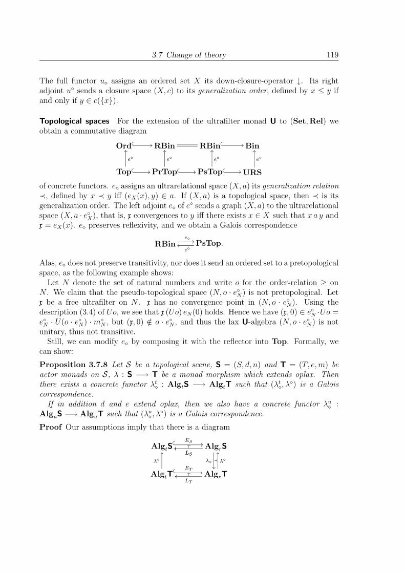
3.7 Change of theory 119
The full functor u assigns an ordered set X its down-closure-operator ↓. Its rightadjoint u sends a closure space (X, c) to its generalization order, defined by x ≤ y ifand only if y ∈ c({x}).
Topological spaces For the extension of the ultrafilter monad U to (Set,Rel) weobtain a commutative diagram
Ord� � �� RBin RBin
� � �� Bin
Top � � ��
e
��
PrTop � � ��
e
��
PsTop � � ��
e
��
URS
e
��
of concrete functors. e assigns an ultrarelational space (X, a) its generalization relation≺, defined by x ≺ y iff (eX(x), y) ∈ a. If (X, a) is a topological space, then ≺ is itsgeneralization order. The left adjoint e of e sends a graph (X, a) to the ultrarelationalspace (X, a · e◦X), that is, x convergences to y iff there exists x ∈ X such that x a y andx = eX(x). e preserves reflexivity, and we obtain a Galois correspondence
RBine �� PsTop.e
Alas, e does not preserve transitivity, nor does it send an ordered set to a pretopologicalspace, as the following example shows:
Let N denote the set of natural numbers and write o for the order-relation ≥ onN . We claim that the pseudo-topological space (N, o · e◦N) is not pretopological. Letx be a free ultrafilter on N . x has no convergence point in (N, o · e◦N). Using thedescription (3.4) of Uo, we see that x (Uo) eN(0) holds. Hence we have (x, 0) ∈ e◦N ·Uo =e◦N · U(o · e◦N) · m◦
N , but (x, 0) /∈ o · e◦N , and thus the lax U-algebra (N, o · e◦N) is notunitary, thus not transitive.
Still, we can modify e by composing it with the reflector into Top. Formally, wecan show:
Proposition 3.7.8 Let S be a topological scene, S = (S, d, n) and T = (T, e,m) beactor monads on S, λ : S −→ T be a monad morphism which extends oplax. Thenthere exists a concrete functor λt
: AlgtS −→ AlgtT such that (λt , λ
) is a Galoiscorrespondence.
If in addition d and e extend oplax, then we also have a concrete functor λu :
AlguS −→ AlguT such that (λu , λ
) is a Galois correspondence.
Proof Our assumptions imply that there is a diagram
AlgtS� � ES ��
AlgrSLS
�
LS
λ
��
AlgtT� � ET ��
λ
��
AlgrTLT
λ
��
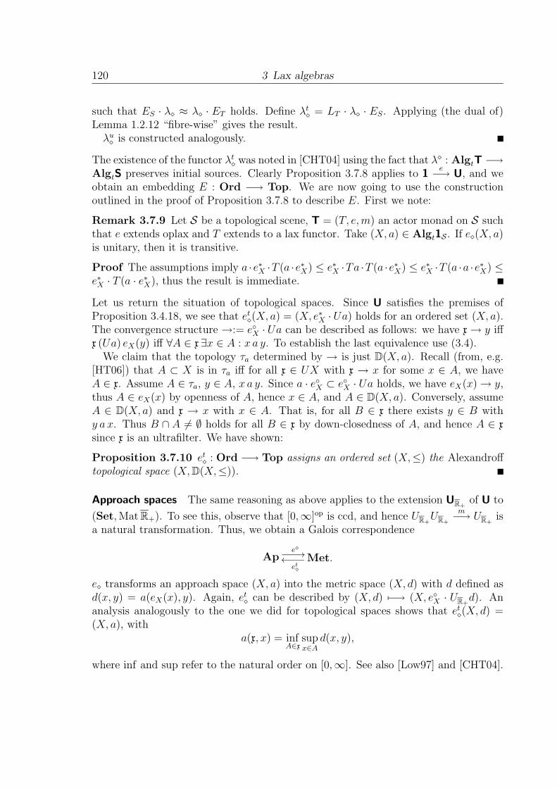
120 3 Lax algebras
such that ES · λ ≈ λ · ET holds. Define λt = LT · λ · ES. Applying (the dual of)
Lemma 1.2.12 “fibre-wise” gives the result.λu is constructed analogously.
The existence of the functor λt was noted in [CHT04] using the fact that λ : AlgtT −→
AlgtS preserves initial sources. Clearly Proposition 3.7.8 applies to 1e−→ U, and we
obtain an embedding E : Ord −→ Top. We are now going to use the constructionoutlined in the proof of Proposition 3.7.8 to describe E. First we note:
Remark 3.7.9 Let S be a topological scene, T = (T, e,m) an actor monad on S suchthat e extends oplax and T extends to a lax functor. Take (X, a) ∈ Algt1S . If e (X, a)is unitary, then it is transitive.
Proof The assumptions imply a ·e∗X ·T (a ·e∗X) ≤ e∗X ·Ta ·T (a ·e∗X) ≤ e∗X ·T (a ·a ·e∗X) ≤e∗X · T (a · e∗X), thus the result is immediate.
Let us return the situation of topological spaces. Since U satisfies the premises ofProposition 3.4.18, we see that et
(X, a) = (X, e∗X ·Ua) holds for an ordered set (X, a).The convergence structure →:= e◦X · Ua can be described as follows: we have x→ y iffx (Ua) eX(y) iff ∀A ∈ x∃x ∈ A : x a y. To establish the last equivalence use (3.4).
We claim that the topology τa determined by → is just D(X, a). Recall (from, e.g.[HT06]) that A ⊂ X is in τa iff for all x ∈ UX with x → x for some x ∈ A, we haveA ∈ x. Assume A ∈ τa, y ∈ A, x a y. Since a · e◦X ⊂ e◦X · Ua holds, we have eX(x) → y,thus A ∈ eX(x) by openness of A, hence x ∈ A, and A ∈ D(X, a). Conversely, assumeA ∈ D(X, a) and x → x with x ∈ A. That is, for all B ∈ x there exists y ∈ B withy a x. Thus B ∩ A �= ∅ holds for all B ∈ x by down-closedness of A, and hence A ∈ x
since x is an ultrafilter. We have shown:
Proposition 3.7.10 et : Ord −→ Top assigns an ordered set (X,≤) the Alexandroff
topological space (X, D(X,≤)).
Approach spaces The same reasoning as above applies to the extension UR+of U to
(Set, Mat R+). To see this, observe that [0,∞]op is ccd, and hence UR+UR+
m−→ UR+
isa natural transformation. Thus, we obtain a Galois correspondence
Ape ��
Met.et
e transforms an approach space (X, a) into the metric space (X, d) with d defined asd(x, y) = a(eX(x), y). Again, et
can be described by (X, d) �−→ (X, e◦X · UR+d). An
analysis analogously to the one we did for topological spaces shows that et (X, d) =
(X, a), witha(x, x) = inf
A∈xsupx∈A
d(x, y),
where inf and sup refer to the natural order on [0,∞]. See also [Low97] and [CHT04].
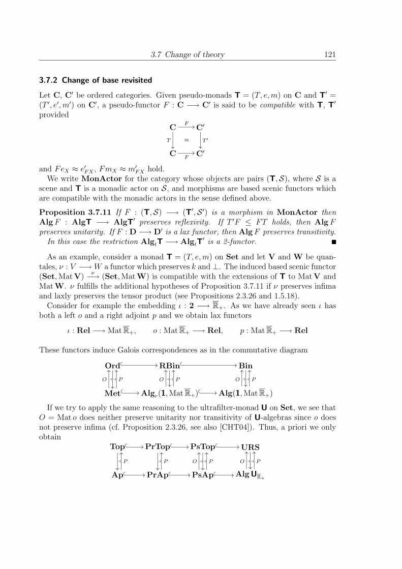
3.7 Change of theory 121
3.7.2 Change of base revisited
Let C, C′ be ordered categories. Given pseudo-monads T = (T, e,m) on C and T′ =(T ′, e′,m′) on C′, a pseudo-functor F : C −→ C′ is said to be compatible with T, T′
provided
CF ��
T��
≈
C′
T ′
��
CF
�� C′
and FeX ≈ e′FX , FmX ≈ m′FX hold.
We write MonActor for the category whose objects are pairs (T,S), where S is ascene and T is a monadic actor on S, and morphisms are based scenic functors whichare compatible with the monadic actors in the sense defined above.
Proposition 3.7.11 If F : (T,S) −→ (T′,S ′) is a morphism in MonActor thenAlg F : AlgT −→ AlgT′ preserves reflexivity. If T ′F ≤ FT holds, then Alg Fpreserves unitarity. If F : D −→ D′ is a lax functor, then Alg F preserves transitivity.
In this case the restriction AlgtT −→ AlgtT′ is a 2-functor.
As an example, consider a monad T = (T, e,m) on Set and let V and W be quan-tales, ν : V −→W a functor which preserves k and⊥. The induced based scenic functor(Set, MatV)
ν−→ (Set, MatW) is compatible with the extensions of T to MatV and
MatW. ν fulfills the additional hypotheses of Proposition 3.7.11 if ν preserves infimaand laxly preserves the tensor product (see Propositions 2.3.26 and 1.5.18).
Consider for example the embedding ι : 2 −→ R+. As we have already seen ι hasboth a left o and a right adjoint p and we obtain lax functors
ι : Rel −→ Mat R+, o : Mat R+ −→ Rel, p : Mat R+ −→ Rel
These functors induce Galois correspondences as in the commutative diagram
Ord� � ��
��
��
RBin
��
��
� � �� Bin
��
��
Met� � ��
P
��
O
��
Algr(1, Mat R+)� � ��
P
��
O
��
Alg(1, Mat R+)
P
��
O
��
If we try to apply the same reasoning to the ultrafilter-monad U on Set, we see thatO = Mat o does neither preserve unitarity nor transitivity of U-algebras since o doesnot preserve infima (cf. Proposition 2.3.26, see also [CHT04]). Thus, a priori we onlyobtain
Top � � ��
��
�
PrTop � � ��
��
�
PsTop
��
��
� � �� URS
��
��
Ap � � ��
P
��
PrAp � � ��
P
��
PsAp � � ��
P
��
O
��
AlgUR+
P
��
O
��

122 3 Lax algebras
Observe that we obtain concrete left adjoints to the embeddings Top ↪→ Ap and
PrTop ↪→ PrAp by composing Ap ↪→ PsApO−→ PsTop and PrAp ↪→ PsAp
O−→
PsTop with the reflectors PsTop −→ Top and PsTop −→ PrTop, respectively, see[CHT04].

4 Further examples
4.1 Comparing Kleisli-scenes and distributors
Suppose we are given a 2-monad T = (T, e,m) on Ord such that each Tf has a rightadjoint. Proposition 2.3.12 gives an extension of T to an actor onD = (Set,Ord,Dist),which we will simply denote by T . We can now study either
(1) lax algebras for the identity actor on the discrete scene KleiT = (Set,OrdT), or
(2) lax algebras for the actor T on D.
In this section we will compare these lax algebras. As an example, we will study thefilter-on-downsets monad F on Ord. Here (1) leads to the description of topologicalspaces via neighborhood-filters, while (2) leads to the description of topological spacesvia filter-convergence. This example was studied in [HT06].
The embedding
Fix a 2-monad T = (T, e,m) on Ord such that TX is skeletal for each ordered set Xand Tf has a right adjoint for each f in Ord. Under this condition, we can form theKleisli-scene KleiT of T, and define a concrete “comparison” functor
Alg(1, KleiT)K−→ Alg(T,D),
(X,Xa−→ TX) �−→ (X,TX
a∗
−→� X).
Here a∗ is the right adjoint distributor defined by the (monotone) function a, that is,
x a∗x ⇐⇒ x ≤ a(x).
Observe that we have, for any Xa−→ TY , Y
b−→ TZ in Ord,
(b ∗ a)∗ = (mZ · Tb · a)∗ = a∗ · Tb∗ ·m∗Z = a∗ ∗ b∗, (4.1)
where the composition on the right denotes Hofmann’s coKleisli-composition. Thus therestriction of K to the fibers is an anti-homomorphism with respect to the (Kleisli-)composition and the coKleisli-composition, that is, the coKleisli-composition is just theextension “along ( )∗” of the Kleisli-composition to arbitrary distributors. In particular,using “∗” to denote either of them should not cause any confusion.
123

124 4 Further examples
Proposition 4.1.1 K is a full embedding and each K(X, a) is unitary. K(X, a) isreflexive (transitive) if and only if (X, a) is reflexive (transitive). The restriction of Kdefines a locally fully-faithful 2-functor (Algt(1, KleiT))co −→ Algt(T,D).
Proof Let (X, a), (Y, b) ∈ Alg(1, KleiT). A function Xf−→ Y is a KleiT-functor
(X, a) −→ (Y, b) iff Tf ·a ≤ b · f holds in Ord. This is equivalent to (Tf ·a)∗ ≤ (b · f)∗
in Dist, and hence to f∗ ·a∗ ≤ b∗ ·Tf∗ in Dist, that is, to the fact that f is a Alg(T,D)
morphism (X, a∗) −→ (Y, b∗).Since each TX is ordered anti-symmetrically, ( )∗ is an embedding, and thus also K
is one. In OrdT a ∗ eX = a holds trivially, and e∗X ∗ a∗ = a∗ follows by (4.1). ThereforeK(X, a) is unitary.
(X, a) is reflexive iff eX ≤ a holds in Ord, iff e∗X ≤ a∗ holds in Dist, that is, iffK(X, a) is reflexive. Using (4.1), we see that K preserves and reflects transitivity.
Finally, for f, g : (X, a) −→ (Y, b) in Algt(1, KleiT), we have f ⇒ g iff eY · g ≤ b · fpointwise in Ord, iff g∗ · e∗Y ≤ f ∗ · b∗ in Dist, iff f∗ ≤ b∗ · eY · g in Dist, iff g ⇒ f inAlgt(T,D).
We will describe the image of K. Observe that any a∗ has the property that wheneverx ∈ X and A ⊂ TX satisfy a a∗ x for all a ∈ A and
∨A exists in TX, then also
(∨A) a∗ x. This leads us to the following definition due to Seal [Sea05b]:
Definition 4.1.2 Assume TX to be a complete lattice for all X. We call (X, r) ∈Alg(T,O(V)) continuous provided
r(∨A, x) =
∧a∈A
r(a, x) (4.2)
holds for all A ⊂ TX, x ∈ X.
“≤” is always satisfied in (4.2) since r is a distributor. Thus, in case V = 2, (4.2) is infact equivalent to
a r x for all a ∈ A =⇒ (∨A) r x.
Lemma 4.1.3 If TX is complete for all X, then (X, r) ∈ Alg(T,D) is in the im-age of K if and only if it is continuous. Thus K defines an isomorphism betweenAlg(1, KleiT) and the full subcategory of Alg(T,D) spanned by the continuous laxalgebras. In particular, every continuous lax algebra is unitary.
Proof Clearly every K(X, a) is continuous. If (X, r) is continuous, we define a (mono-tone) function X
a−→ TX by a(x) =
∨{ x ∈ TX | x r x }. r = a∗ follows by continuity
of (X, r).
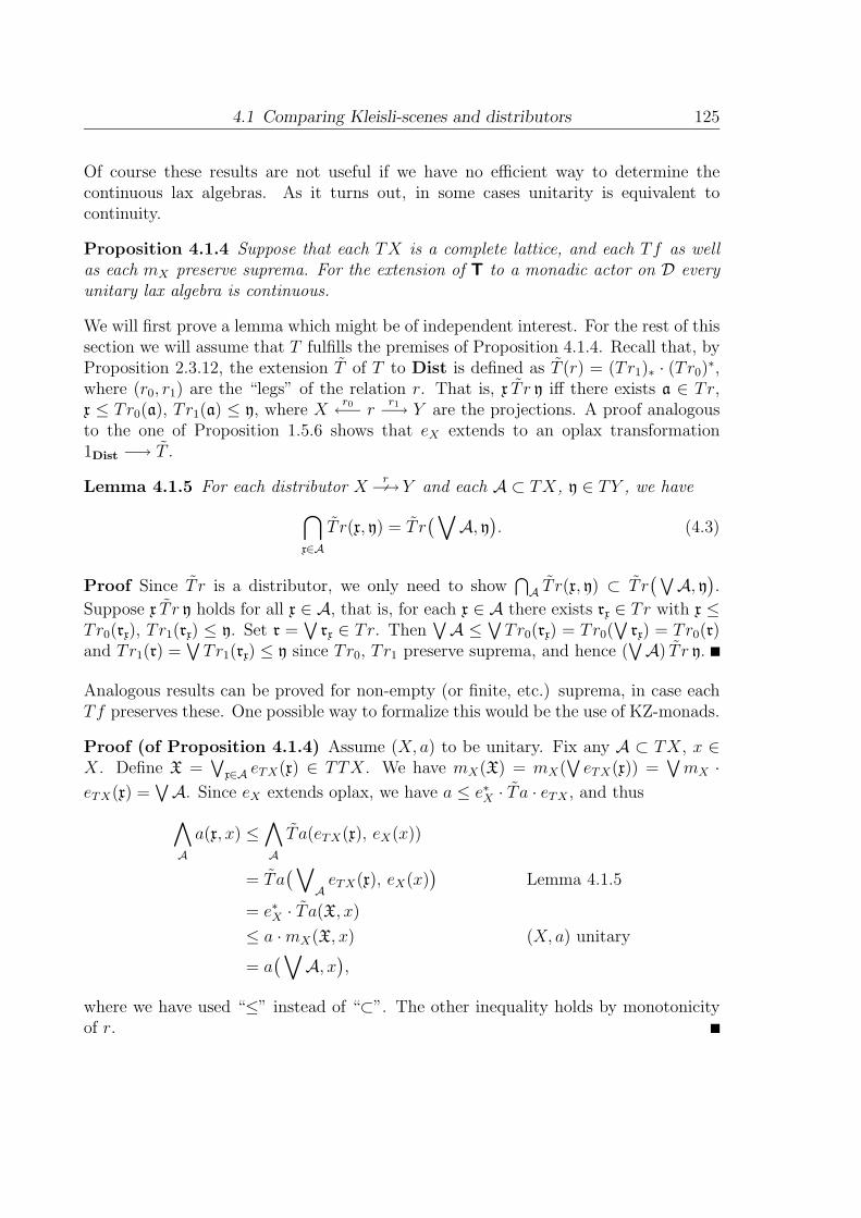
4.1 Comparing Kleisli-scenes and distributors 125
Of course these results are not useful if we have no efficient way to determine thecontinuous lax algebras. As it turns out, in some cases unitarity is equivalent tocontinuity.
Proposition 4.1.4 Suppose that each TX is a complete lattice, and each Tf as wellas each mX preserve suprema. For the extension of T to a monadic actor on D everyunitary lax algebra is continuous.
We will first prove a lemma which might be of independent interest. For the rest of thissection we will assume that T fulfills the premises of Proposition 4.1.4. Recall that, byProposition 2.3.12, the extension T of T to Dist is defined as T (r) = (Tr1)∗ · (Tr0)
∗,where (r0, r1) are the “legs” of the relation r. That is, x T r y iff there exists a ∈ Tr,x ≤ Tr0(a), Tr1(a) ≤ y, where X
r0←− rr1−→ Y are the projections. A proof analogous
to the one of Proposition 1.5.6 shows that eX extends to an oplax transformation1Dist −→ T .
Lemma 4.1.5 For each distributor Xr−→� Y and each A ⊂ TX, y ∈ TY , we have⋂
x∈A
T r(x, y) = T r(∨
A, y). (4.3)
Proof Since T r is a distributor, we only need to show⋂
A T r(x, y) ⊂ T r(∨
A, y).
Suppose x T r y holds for all x ∈ A, that is, for each x ∈ A there exists rx ∈ Tr with x ≤Tr0(rx), Tr1(rx) ≤ y. Set r =
∨rx ∈ Tr. Then
∨A ≤
∨Tr0(rx) = Tr0(
∨rx) = Tr0(r)
and Tr1(r) =∨
Tr1(rx) ≤ y since Tr0, Tr1 preserve suprema, and hence (∨A) T r y.
Analogous results can be proved for non-empty (or finite, etc.) suprema, in case eachTf preserves these. One possible way to formalize this would be the use of KZ-monads.
Proof (of Proposition 4.1.4) Assume (X, a) to be unitary. Fix any A ⊂ TX, x ∈X. Define X =
∨x∈A eTX(x) ∈ TTX. We have mX(X) = mX(
∨eTX(x)) =
∨mX ·
eTX(x) =∨A. Since eX extends oplax, we have a ≤ e∗X · T a · eTX , and thus∧A
a(x, x) ≤∧A
T a(eTX(x), eX(x))
= T a(∨
AeTX(x), eX(x)
)Lemma 4.1.5
= e∗X · T a(X, x)
≤ a ·mX(X, x) (X, a) unitary
= a(∨
A, x),
where we have used “≤” instead of “⊂”. The other inequality holds by monotonicityof r.
126 4 Further examples
The following result follows immediately from Propositions 4.1.1 and 4.1.4:
Theorem 4.1.6 If T fulfills the conditions of Proposition 4.1.4, then Alg(1, KleiT)is, via K, concretely isomorphic to the full subcategory of Alg(T,D) spanned by theunitary lax algebras. Moreover, K restricts to concrete isomorphisms
Algr(1, KleiT) ∼= Algu(T,D), Algt(1, KleiT) ∼= Algt(T,D).
A counterexample Let U be the upper-set monad on Ord. The extension of thefunctor U to Dist is a 2-functor, each UX is complete, and each mX : UUX −→ UXpreserves suprema. We have seen (Remark 3.4.11) that every lax U-algebra is unitary.
But Proposition 4.1.4 does not apply. Although every Uf has a left adjoint, it doesnot in general preserve suprema.
On the other hand, a (not necessarily reflexive or transitive) lax algebra for U on aset X is just a “monotone operator” c : PX −→ PX, and continuity of the algebrameans that for every x ∈ X there is a smallest (w.r.t. ⊂) A ⊂ X with x ∈ cA. Thusthe category of continuous lax algebras for U is the category Bin of thin graphs.
4.2 Level algebras and tower-extensions
Let V be a non-trivial quantale and fix a monadic actor T = (T, e,m) on D. We denotethe extension of T to O(V) defined in Section 2.3.4 by TV.
Level algebras Recall that for a V-matrix a : X −→� Y , we denote by av ⊂ X × Ythe level -relation defined by x av y if and only if v ≤ a(x, y).
Proposition 4.2.1 For v ∈ V the assignment (X, a) �−→ (X, av) defines a concretefunctor Lv : Alg TV −→ Alg T . We call Lv(X, a) the level-algebra of (X, a) at v.
Proof First recall that av is a distributor provided a is an ordered matrix. Suppose
that (X, a)f−→ (Y, b) is a morphism in AlgTV, that is, f∗ · a ≤ b · Tf∗. Then,
f∗ · av ⊂ (f∗ · a)v Lemma 2.3.13(3)
⊂ (b · Tf∗)v assumption and Lemma 2.3.13(1)
= (b · Tf)v since b is an ordered matrix
= bv · Tf Lemma 2.3.13(4)
= bv · Tf∗ since bv is a distributor.
Proposition 4.2.2 The following statements hold:
(1) If each TX is complete, then every Lv preserves continuity of lax algebras;

4.2 Level algebras and tower-extensions 127
(2) Lv preserves reflexivity if and only if v ≤ kV;
(3) (X, a) in AlgTV is unitary if and only if (X, av) is unitary for each v ∈ V .
Proof Let (X, a) be a lax TV-algebra.
[1] Suppose that (X, a) is continuous and A ⊂ TX. Assume x av x for all x ∈ A. Thenv ≤∧
x∈A a(x, x) = a(∨A, x) by continuity.
[2] For v ≤ kV preservation of reflexivity follows from Remark 2.3.14. Conversely,let X = {x} and take any v ∈ V . If Lv preserves reflexivity, then in particularLv(X, e∗X) is reflexive, and v ≤ e∗X(eX(x), x) = kV holds.
[3] “Only if” is obvious. For the converse implication take any X ∈ TTX and x ∈ X.Since a and TVa are distributors we only need to show that TVa(X, eX(x)) ≤a(mX(X), x) holds. By definition of TV it suffices to show v ≤ a(mX(X), x) for allv ∈ V with XTav eX(x). Take any such v. Since (X, av) is unitary by assumptionwe obtain mX(X) av x, equivalently, v ≤ a(mXX, x).
Lv does not need to preserve transitivity. Consider for instance the metric space (X, d)given by X = {x, y, z } and
d x y z
x 0 2 3y 2 0 2z 3 2 0
Since (recall the order on R+) x dr y iff d(x, y) ≤ r for all r ∈ R+, we have x d2 y, y d2 z,but x �d2 z, and thus d2 is not transitive.
Continuity for actors on O(V) For this section, additionally assume T to be a 2-monad on Ord such that TX is a complete lattice for all ordered sets X and that allTf and mX preserve suprema.
Proposition 4.2.3 Every continuous lax TV-algebra (X, a) is unitary.
Proof Suppose (X, a) to be continuous. Then each Lv(X, a) is continuous by Proposi-tion 4.2.2(1). By Proposition 4.1.4, each Lv(X, a) is unitary, and thus, by Proposition4.2.2(3), also (X, a) is unitary.
Lemma 4.2.4 If V is ccd, we have∧x∈A
TVa(x, y) = TVa(∨
A, y)
for each distributor Xa−→� Y and all A ⊂ TX, y ∈ TY .

128 4 Further examples
Proof Since TV is a distributor, we only have to show “≤”. As usual, we writeB − �
∨: DV −→ V . With αx := TVa(x, y) and W := { v ∈ V |
∨A T av y } we need
to show∧
x∈A αx ≤∨
W , equivalently B(∧
αx) ⊂ W . Take v ∈ B(∧
A αx) ⊂⋂
A B(αx).
We have to show∨A T av y.
For each x ∈ A, we have v ≤ αx =∨{w ∈ V | x T aw y }, which together with
v ∈ B(αx) implies x T av y. Since (4.3) holds for T av, we thus have v ∈W .
Theorem 4.2.5 Assume V to be ccd. An algebra in Alg(TV,O(V)) is continuous ifand only if it is unitary.
Proof The proof of Proposition 4.1.4 (with Lemma 4.2.4 instead of Lemma 4.1.5) gives“if”. “Only if” follows from Proposition 4.2.3.
Tower extensions
We recall the notion of tower-extension from [Zha00]:
Definition 4.2.6 Let XP−→ B be a fiber-small topological functor and V be a com-
plete lattice. The tower-extension X[V ] of X by V is defined as the following category:
• objects are towers of X-objects, that is, pairs (B, φ), where B is an object of Band φ : V −→ P op
B preserves suprema;
• a morphism (B, φ)f−→ (B′, φ′) is given by a B-morphism f : B −→ B′ such that
φ(v)f−→ φ′(v) is an X-morphism for all v ∈ V .
Here, P opB is the fiber of P over B, ordered by X ≤ X ′ iff X ′ 1B−→ X is an X-morphism.
X[V ] becomes a concrete category by the obvious forgetful functor X[V ] −→ B. Fora tower (X,φ), we call φ(v) the component of (X,φ) at v ∈ V . Assigning a tower itsv-component defines the concrete component-functors Cv : X[V ] −→ X.
Since the powerset PA is the free Sup-lattice on a set A, we can describe X[PA] asfollows: objects are pairs (B, (Xa)A), where B is a B-object and (Xa) is an A-indexedfamily of X-objects over B. Morphisms f : (B, (Xa)) −→ (B′, (X ′
a)) are B-morphismsf : B −→ B′ such that f : Xa −→ X ′
a is an X-morphism for all a ∈ A. In particular,for the two-element chain 2, we have a concrete isomorphism X[2] ∼= X.
Lax algebras are tower extensions Fix a 2-monad T = (T, e,m) on Ord. As usual,TV denotes the extension of T to O(V) for a quantale V. Although we will formulatethe results in this section for scenes of the type O(V), all of them remain valid over(Set, MatV).
We can, by Lemma 2.3.13(1) and Proposition 4.2.1, define a concrete functor
G : Alg TV −→ Alg T [V ], (X, a) �−→ (X, (v �→ av)).

4.2 Level algebras and tower-extensions 129
Proposition 4.2.7 G is an isomorphism and for each v ∈ V the following diagramcommutes:
Alg TVG ��
Lv ������
������
Alg T [V ]
Cv$$������
����
Alg T
Proof G−1 sends (X,φ) to (X, Γφ), where Γφ(x, x) =∨{ v ∈ V | xφ(v) x }. Clearly
G−1 is functorial.We have Γ(v �→ av)(x, x) =
∨{w ∈ V | x aw x } = a(x, x) for each V-matrix a, thus
G−1G = 1. Now let φ : V −→ (Dist(TX, T ))op preserve suprema. We need to show(Γφ)v = φ(v) for each v ∈ V . Clearly, φ(v) ⊂ (Γφ)v holds. Take x ∈ X, x ∈ TX andwrite W = { v ∈ V | xφ(v) x }. W is a downset, and since φ preserves suprema we have(x, x) ∈ φ(
∨W ), thus
∨W ∈ W . Hence, v ≤
∨W implies v ∈ W , and (Γφ)v ⊂ φ(v)
follows.
Proposition 4.2.8 For (X,φ) ∈ Alg T [V ], we have:
(1) G−1(X,φ) ∈ Alg TV is reflexive if and only if (X, (φ(k)) ∈ Alg T is reflexive.
(2) G−1(X,φ) ∈ Alg TV is unitary if and only if for each v ∈ V , (X,φ(v)) ∈ Alg T isunitary.
Proof Follows from 4.2.2(2) and (3).
Corollary 4.2.9 Let V be integral. G and G−1 restrict to concrete isomorphisms
AlgrTV∼= AlgrT [V] and AlguTV
∼= AlguT [V].
Proposition 4.2.10 Let (X, a) ∈ Alg TV be transitive. For each u, v ∈ V we haveau ∗ av ⊂ au⊗v, where ∗ denotes the coKleisli-composition.
Proof Recall that T (av) ⊂ (TVa)v holds for v ∈ V . Hence, it suffices to show au ·(TVa)v ⊂ au⊗v ·mX . Take any X ∈ TTX, x ∈ X, and assume X (au · (TVa)v) x. Thus,there exists x ∈ TX with u ≤ a(x, x) and v ≤ TVa(X, x). In particular,
u⊗ v ≤∨
x∈TX
a(x, x)⊗ TVa(X, x) = a · TVa(X, x) ≤ a ·mX(X, x).
Since (a ·mX)u⊗v = au⊗v ·mX holds, we are done.
The two preceding results motivate the following definition:
Definition 4.2.11 Let us call (X,φ) ∈ Alg T [V ]

130 4 Further examples
• coherent if φ(u) ∗ φ(v) ⊂ φ(u⊗ v) holds for all u, v ∈ V , and
• normal if e∗X ⊂ φ(kV) holds.
Thus (X,φ) is normal and coherent iff φ : V −→ Dist(TX,X)op is a lax monoidalfunctor, where Dist(TX,X) has the (not necessarily associative) coKleisli-compositionas “tensor”. Normality of (X,φ) is equivalent to reflexivity of (X,φ(v)) for all v ≤ kV.
Observe that if (X,φ) is coherent then (X,φ(u)) is transitive for all idempotentu ∈ V . In particular, (X,φ(k)) is transitive. In case V is a frame, we even have:
Lemma 4.2.12 Assume that V is a frame, that is, ⊗ = ∧ holds. Then (X,φ) ∈Alg T [V ] is coherent if and only if each (X,φ(v)) is transitive.
Proof “Only if” is obvious. To prove “if” take any u, v ∈ V . Write w = u ∧ v, thusφ(u) ⊂ φ(w) and φ(v) ⊂ φ(w) hold. This implies φ(u) ∗ φ(v) ⊂ φ(w) ∗ φ(w) ⊂ φ(w) =φ(u ∧ v).
Proposition 4.2.13 A lax algebra (X, a) in Alg TV is transitive if and only if G(X, a)is coherent. Thus G and G−1 restrict to isomorphisms between the full subcategory ofAlg TV spanned by the transitive lax algebras and the full subcategory of Alg T [V ]spanned by the coherent towers.
Proof Assume G(X, a) = (X, (av)V ) to be coherent. Clearly, it suffices to showa(x, x) ⊗ TVa(X, x) ≤ a(mX(X), x) for all X ∈ TTX, x ∈ TX, x ∈ X. Let us fixsuch X, x, x, and write u = a(x, x), W = {w ∈ V | XTaw x }. We have
a(x, x)⊗ TVa(X, x) = u⊗∨
W =∨
w∈W
u⊗ w.
But for any w ∈ W , we have (X, x) ∈ au·Taw = φ(u)·Tφ(w) ⊂ φ(u⊗w)·mX = au⊗v·mX ,thus u⊗ w ≤ a(mX(X), x), and the claim is proved.
The converse implication follows from Proposition 4.2.10.
We summarize our results in the following theorem, which characterizes reflexive andtransitive lax TV-algebras in terms of towers:
Theorem 4.2.14 AlgtTV is concretely isomorphic to the full subcategory of Alg T [V ]spanned by the normal and coherent towers. If V is integral, then AlgtTV is concretelyisomorphic to the full subcategory of AlgrT [V ] spanned by the coherent towers.
In particular, if (X,φ) ∈ Alg T [V ] is normal and coherent, then each (X,φ(v)) isunitary.
Corollary 4.2.15 If ⊗ idempotent, then each Lv preserves transitivity. Moreover,⊗ = ∧ implies AlgtT[V ] ∼= AlgtTV.
Proof Follows immediately from Lemma 4.2.12.
The result of this section were — in a slightly different setting — proved indepen-dently by Seal in [Sea05b], under the additional hypothesis that V is ccd. Seal wasfirst to recognize the importance of what we choose to call normal towers.

4.3 An example: topological spaces via filter convergence 131
4.3 An example: topological spaces via filter convergence
The goal of this section is to show how topological spaces can be described as laxalgebras using filter-convergence instead of ultrafilter-convergence, thereby avoidingthe use of the Axiom of Choice. For other approaches to the same characterization,see [Wyl91], [Pis99], [HT06], [Sea05a].
Let F = (F, e,m) be the filter-on-downsets monad on Ord. We have seen in Section1.3.6 that F satisfies the premises of Theorem 4.1.6, which gives concrete isomorphismsAlgr(1, KleiF) ∼= Algu(F,D) and Algt(1, KleiF) ∼= Algt(F,D). Since, by Proposition1.6.15, we have Algt(1, KleiF) ∼= Top, and moreover Algr(1, KleiF) ∼= PrTop (cf.Section 3.4.2), we have shown
Theorem 4.3.1 We have concrete isomorphisms Algu(F,D) ∼= PrTop, Algt(F,D) ∼=Top.
Clearly, Algr(F,D) is just the category Conv of (filter) convergence spaces (in thesense of, e.g., [Wyl91]). Thus our typical string (3.3) of lax algebras can for F bedescribed as:
Top ↪−→ PrTop ↪−→ Conv ↪−→ AlgF.
4.3.1 Extending the filter-functor to Dist
Although we did not need an explicit description of the extension of F to Dist toapply Theorem 4.1.6, we will now give one for further reference. As it turns out, thisextension is a 2-functor.
Given a relation r ⊂ X × Y and B ⊂ Y , we write r�B for r◦[B] = {x ∈ X | ∃b ∈B : x r b }. Observe that r�B is a downset for any subset B ⊂ Y if r is a distributor.
In particular, ≤� B = B↓ is the down-closure of B, and if Xf−→ Y is monotone and
B ∈ DY , then f�
∗ B = f−1[B].We define F : Dist −→ Dist by
xFr y ⇐⇒ ∀B ∈ y : r�B ∈ x, (4.4)
for any distributor Xr−→� Y .
Lemma 4.3.2 F is a 2-functor Dist −→ Dist and the following diagram commutes.
Ord
F��
( )∗�� Dist
F��
Ord( )∗
�� Dist
(4.5)

132 4 Further examples
Proof The identity on X is given by the order-relation≤X and we have xF (≤X) y ⇐⇒∀B ∈ y : B ∈ x ⇐⇒ x ≤ y for all x, y ∈ FX, thus F preserves identities.
To show that F preserves composition, let Xr−→� Y
s−→� Z be distributors and x ∈
FX, z ∈ FZ. Then
xF (s · r) z ⇐⇒ ∀C ∈ z : r�(s�C) ∈ x, (4.6)
and
x (Fs · Fr) z ⇐⇒ ∃y ∈ FY : xFr y, y Fs z
⇐⇒ ∃y ∈ FY ∀B ∈ y∀C ∈ z r�B ∈ x, s�C ∈ y.
Thus clearly Fs ·Fr ⊂ F (s · r) holds. To show the converse, suppose that for all C ∈ z,r�(s�C) ∈ x. Define b ⊂ DY as b = {B | ∃C ∈ z : B = s�C }. Clearly b is filtered,and hence y = b↑ ∈ FY . For each C ∈ z, s�C ∈ y holds by construction. On the otherhand, for each B ∈ y, there exists C ∈ z with s�C ⊂ B, thus r�(s�C) ⊂ r�B, andhence r�B ∈ x by assumption. We have proved F (s · r) ⊂ Fs · Fr.
That F is locally monotone and makes (4.5) commutative is obvious.
4.3.2 Other topological constructs via filter convergence
For a quantale V let FV denote the extension of F to a monadic actor on O(V), formed
by extending DistF−→ Dist to an actor on O(V) according to the recipe of Section
2.3.4. We are going to describe the corresponding categories of lax algebras.
Approach spaces
Take V = R+ = ([0,∞]op, +, 0) (cf. Examples 1.5.8(3)). Observe that [0,∞] (andhence [0,∞]op) is ccd: the left adjoint B of
∨is given by B(a) = { b ∈ [0,∞] | b < a }.
Proposition 4.3.3 We have concrete isomorphisms
AlguFR+
∼= PrAp and AlgtFR+
∼= Ap,
where PrAp is the category of pre-approach spaces and contractions and Ap is thefull subcategory of approach spaces.
Proof We have AlguFR+
∼= AlguF[R+] ∼= PrTop[R+]. By a result of Brock and Kent
[BK97, Proposition 10] (see also [Zha00]) PrTop[R+] is isomorphic to PrAp.Observe that by Theorem 4.2.14, (X, a) ∈ AlgtFR+
is completely determined by a[0,∞]-indexed family of pretopologies, which we describe as interior-operators iε, onX such that i∞ is the discrete pretopology, we have iε =
⋂γ>ε iγ (here we make use of
Remark 1.3.8) and iε · iγ ⊂ iε+γ (here we use Lemma 1.6.16). But this data constitutesprecisely the data used in [Low97] to define an approach space.
4.4 Back to Kleisli 133
Remark 4.3.4 Using Theorem 4.2.5 we can give a slightly different proof of the firstisomorphism in Proposition 4.3.3: simply observe that, via Theorem 4.2.5 for a lax FR+
-algebra (X, a) unitarity is equivalent to continuity, and continuity is precisely condition(PRAL) of [LL89].
Remark 4.3.5 Almost the same reasoning as in the proof of Proposition 4.3.3 can beemployed to prove statements (2) and (3) of Theorem 3.4.5. In place of Lemma 1.6.16one has to use [HT06, Theorem D].
Other examples
Using the results of Zhang [Zha00] on tower extensions and our description of laxalgebras over the scenes O(V) and (Set, MatV) we obtain descriptions of variouscategories of lax algebras. For instance, we have for V = ([0, 1],∧, 1)
• AlgrU[0,1] is concretely isomorphic to the category of probabilistic pseudotopolog-ical spaces of [BK97];
• AlguF[0,1] and AlguU[0,1] are concretely isomorphic to the category of probabilisticpretopological spaces of [BK97];
• AlgtF[0,1] and AlgtU[0,1] are concretely isomorphic to the category of probabilistictopological spaces of [BK97].
For more examples see [Zha00]. In all cases the proofs are routine using the methodsalready employed for the corresponding results concerning approach spaces. For anexample which is not a chain, consider V = 22 ∼= P2. We have AlgtF22
∼= AlgtU22∼=
BiTop, the category of bitopological spaces. This was first observed by G. Seal (per-sonal communication, September 2006).
4.4 Back to Kleisli
We have seen in Section 4.1 that for a 2-monad T on Ord there is a concrete isomor-phism between Cat KleiT and the category and reflexive and transitive lax algebrasfor the canonical extension of T to an actor on D, provided each TX is completeand, crucially, each Tf and each mX preserve suprema. Thus suitable completenessproperties allow us to switch from a “neighborhood”-point of view (Kleisli-scenes) to a“convergence”-point of view (distributors), and vice versa. This correspondence breaksdown if Tf does not preserve suprema, as we have seen for the upper-set monad U.
We will now present a construction which allows us to complete a monad, so that theabove-mentioned correspondence holds. In particular, we get a “neighborhood”-versionof closure spaces. Our method is inspired by Seal’s [Sea05b] use of up-closed familiesof subsets.

134 4 Further examples
The setting Fix a 2-monad D = (D, d, n) on Ord such that each Df has a rightadjoint D∗f and each nX has a right adjoint n∗
X . We form the Kleisli-scene K(D) =(Set,Ord,Ordop
D ). For simplicity, we write D = OrdopD . Let T = (T, e,m) be any
2-monad on Ord which extends to a 2-monad along ( )∗ = FD : Ord −→ D. That is,there exists a 2-functor T : D −→ D such that T = (T , (e∗X)X , (m∗
X)X) is a 2-monadon OrdD and T · FD = FD · T holds.
The construction By Proposition 2.3.33 there exists a distributive law λ of T overD such that T = Tλ. Using λ, we form the composite monad S = (S, s, r) = (DT)λ.
Lemma 4.4.1 Each Sf and each rX has a right adjoint.
Proof A right adjoint of Sf = DTf is given by D∗(Tf), and a right adjoint ofrX = DmX · nTTX ·DλTX is given by r∗X = D∗(λTX) · n∗
TTX ·D∗(mX).
Hence we can form the Kleisli-scene K(S). For this, we obtain:
Theorem 4.4.2 There are concrete isomorphisms
Algu(S,D) ∼= Algr(1,K(S)) ∼= Algu(T,K(D)),
Algt(S,D) ∼= Algt(1,K(S)) ∼= Algt(T,K(D)).
Proof The isomorphisms on the left-hand side follow from Theorem 4.1.6. By Lemma2.3.34 we have OrdS
∼= (OrdD)Tλ∼= (OrdD)T, from which the other isomorphisms
follow immediately.
4.4.1 An example: closure spaces via neighborhoods
We will apply this method to D = D, thus K(D) ∼= D, and T = U. The upper-setmonad U has an extension to a 2-monad on OrdD, which was constructed using thedistributive law r. With the help of r, we define the monad DU = (DU)r, which wasalready studied in Section 1.3.1. We recall that Algt(U,D) is the category Clos ofclosure spaces. Hence Theorem 4.4.2 implies
Clos ∼= Cat Klei DU.
We would like to point out that the results of Section 4.2 allow us deduce Seal’s de-scription [Sea05b] of AlgtUV as V-graded family of closure operators for any (notnecessarily ccd) quantale V. Indeed, Seal’s result follows immediately from Theorem4.2.14 using Lemma 3.4.8 and Remark 1.3.8.
In the special case of V being a frame and the underlying lattice V being ccd, U
extends also to a 2-monad on OrdDV
∼= OrdMat(V)op. Thus we obtain a compositemonad DVU and concrete isomorphisms
Cat Klei DVU ∼= Algt(U,O(V)) ∼= Algt(U,D)[V ] ∼= Clos(V),

4.4 Back to Kleisli 135
where the last category denotes Seal’s V-graded closure spaces; see [Sea05b]. Hence,not only the category of closure spaces can be described by “neighborhoods”, but alsothe category of V-valued closure spaces, equivalently, of V-graded closure operators[Sea05b], in case V is a ccd frame.
4.4.2 Algebraic closure spaces
Let Uω be the finitely generated upper-set KZ-monad on Ord, and i : Uω −→ U the
natural inclusion. The restriction UωDrω
−→ DUω provides us with an extension Uω ofUω to Dist. We will describe the lax algebras for it.
The natural embedding i : Uω ↪−→ U extends by Remark 2.3.35 to a natural trans-formation i∗ : U −→ Uω and hence an induces a full embedding
Alg Uωi−→ Alg U,
which by Proposition 3.7.5 preserves and reflects both reflexivity and transitivity. Thuswe obtain the following commutative diagram of full embeddings
AlgtUω��
i
��
AlgrUω
i��
�� Alg Uω
i��
Clos �� AlgrU�� Alg U
Thus, to describe AlgtUω, we just need to characterize those closure spaces which formthe image of i : AlgtUω −→ Clos.
This is done easily: (X,PXr−→� X) is in the image iff r factors as r = r′ · i∗X . Any
such factorization is unique. Thus (X, r) is in the image iff whenever Ar x, there existsa finite subset F ⊂ A with F r′ x. Then clearly F r x. Thus, in the language of closureoperators, with cr(A) = {x ∈ X | Ar x }:
x ∈ cr(A) ⇐⇒ ∃F ⊂ A, F finite, x ∈ cr(F ).
That is, AlgtUω is precisely the category AClos of algebraic closure operators.
Corollary 4.4.3 I : AClos ↪−→ Clos is concretely coreflective.
Proof A concrete right adjoint of I = i is given by i . By Proposition 3.7.5 i
preserves reflexivity and transitivity.
The distributive law rω allows us to construct the composite monad DUω, and Theorem4.4.2 gives
Cat Klei DUω∼= AClos,
that is, also algebraic closure spaces may be described by a suitable type of “neighbor-hoods”.
We note that OrdDUω is just the category of frames [MRW02, 5.7].

136 4 Further examples
4.4.3 Grounded closure spaces
We can repeat the above discussion for the inclusion j : U0 −→ U of the non-emptyuppersets into U. As above, j induces a full embedding j : Alg U0 −→ Alg U whichpreserves reflexivity and transitivity, and we end up with the problem of describing theimage of the restriction i : AlgtU0 −→ Clos.
Since (X, r) is in the image precisely when r factors as r = r′ · j∗X , we see that Ar xiff there exists a non-empty B ⊂ A with B r x. Thus, (X, r) is in the image preciselywhen cr(∅) = ∅ holds.
Let us call a closure space (X, c) grounded if c∅ = ∅ holds, and denote the fullsubcategory of Clos spanned by the grounded closure spaces by GClos. We have, bythe above considerations:
Proposition 4.4.4 GClos concretely isomorphic to AlgtU0. Thus the full embeddingGClos ↪−→ Clos is concretely coreflective.
For the composite monad DU0, we obtain GClos ∼= Cat Klei DU0.Since U0 as well as Uω extend also to 2-comonads on OrdMat(V) for any ccd frame
V, one can also describe frame valued grounded (or algebraic) closure spaces via neigh-borhoods. We refrain from spelling out the details in full.
4.5 The filter construction
Let F be the filter coKZ-monad on Ord. For a locally small, locally finitely completeordered category O we define the filter-category FilO as follows (see also [CH03]):
• obj FilO = objO;
• FilO(A,B) = F(O(A,B)); thus F ≤ F ′ iff F ⊃ F ′;
• the identity on A is given by 1↑A = { f ∈ O(A,A) | 1A ≤ f };
• the composite of G and F is defined to be the filter generated by { g · f | f ∈F, g ∈ G }.
For any f ∈ O(A,B), let f ↑ = {h ∈ O(A,B) | f ≤ h }.
Remark 4.5.1 G · f ↑ = { g · f | g ∈ G }↑ and h↑ ·G = {h · g | g ∈ G }↑ hold wheneverthe composites are defined.
Hence ( )↑ : O −→ FilO is functorial, moreover
f ≤ g ⇐⇒ g↑ ⊂ f ↑ ⇐⇒ f ↑ ≤ g↑
holds, so ( )↑ is locally fully-faithful, in particular a pseudo-functor and hence preservesadjoint situations: (f ↑)∗ ≈ (f ∗)↑ holds for any f ∈ MapO.
4.5 The filter construction 137
The construction of FilO is closely related to the local completion of O constructedin [FS90, 2.221]. Indeed, the local completion, which is the free quantaloid of a locallysmall ordered category, is defined as above, using D in place of F. The author does notknow whether (the embedding of O into) FilO satisfies any universal property.
Remark 4.5.2 F ≤ G ⇐⇒ G ⊂ F ⇐⇒ ∀g ∈ G∃f ∈ F : f ≤ g holds.
Lemma 4.5.3 FilO is locally complete. Given (Fi)I ⊂ FilO(A,B), the infimum is thefilter generated by
⋃I Fi and their supremum is the intersection
⋂I Fi. In particular,
we have
f ∈ (F1 ∧ F2) ⇐⇒ ∃f1 ∈ F1, f2 ∈ F2 : f1 ∧ f2 ≤ f, (4.7)
hence ( )↑ : O −→ FilO locally preserves finite infima and arbitrary suprema.
Let O and O′ be locally finitely complete, locally small ordered categories. For any2-graph morphism T : O −→ O′, we define a 2-graph morphism FilT : FilO −→ FilO′
by
Fil T (X) = T (X), Fil T (F ) = {Tf | f ∈ F }↑.
Proposition 4.5.4 Fil is 2-functorial in the following sense: We have Fil(1O) = 1FilO,Fil(TS) = Fil T · Fil S for any 2-graph morphism T , S, and
O( )↑
��
T��
FilO
Fil T��
O′( )↑
�� FilO′
commutes. If T is a lax functor (an oplax functor, a pseudo-functor, respectively), then
Fil T is a lax functor (an oplax functor, a 2-functor, respectively). If Tλ−→ T ′ is a lax
(oplax, pseudo-natural, respectively) transformation, then (λ↑X)X forms a lax (oplax,
pseudo-natural, respectively) transformation Fil T −→ Fil T ′.
In particular, if O has an involution ( )◦ we can define an involution, also denoted by( )◦, on FilO by F ◦ = {f ◦ | f ∈ F}. Using this notion of involution, we can prove:
Lemma 4.5.5 FilO is an allegory provided O is an allegory.
Although ( )↑ : O −→ FilO is only an embedding if O is locally separated, we identifyan O-morphism with its ( )↑-image.
Lemma 4.5.6 Let M be a class of maps in O. The (co-)Frobenius law holds in (O,M)if and only if the (co-)Frobenius law holds in (FilO,M).
138 4 Further examples
In case O is even locally complete, we define a 2-graph morphism∧
: FilO −→ Obe X �−→ X, F �−→
∧F . Clearly,
∧·( )↑ ≈ 1O and ( )↑ ·
∧≤ 1FilO hold. For
F ∈ FilO(X,Y ), G ∈ FilO(Y, Z), t ∈ O(X,Z), we have
t ≤∧
G ·∧
F =⇒ ∀g ∈ G, f ∈ F : t ≤ g · f
=⇒ ∀h ∈ (G · F ) : t ≤ h
=⇒ t ≤∧
G · F,
thus∧
: FilO −→ O is a normally lax functor. Moreover, for any map f : X −→ Yin O, we have
(∧
G) · f =∧{ g · f | g ∈ G } =
∧{ g · f | g ∈ G }↑ =
∧(G · f ↑) (4.8)
since ( ) · f preserves infima.Observe that for any 2-graph morphism T : O −→ O′ with O, O′ locally complete
we have T ·∧≤∧·Fil T , that is,
∧is “lax natural”.
Filter-scenes Let S =(
S �� C( )∗
��
( )∗�� D)
be a scene with D locally small and
locally finitely complete. We define the scene FilS by the following diagram:
S �� C( )↑·( )∗
��
( )↑·( )∗�� FilD
Then (1S, 1C, ( )↑) : S −→ FilS is a based scenic functor by construction, for whichwe will just write ( )↑. If D is locally complete, then (1S, 1C,
∧) defines a based scenic
functor FilS −→ S, which we will simply denote by∧
.
Extending scenic functors The following result is immediate from Proposition 4.5.4:
Proposition 4.5.7 Let S, S ′ such that FilS and FilS ′ are defined. For any scenicfunctor (T, U) : S −→ S ′, (T, Fil U) defines a scenic functor FilS −→ FilS ′.
Fix a monadic actor T = ((T, U), e,m) on S. We define FilT = ((T, Fil U), e,m). Wemay rephrase the results obtained so far by saying that ( )↑ : (T,S) −→ (FilT, FilS)and∧
: (FilT, FilS) −→ (T,S) are morphisms in MonAct. Thus we obtain con-crete functors E = Alg( )↑ : Alg(T,S) −→ Alg(FilT, FilS) and M = Alg
∧:
Alg(FilT, FilS) −→ Alg(T,S). We summarize their properties in the following re-mark:
Remark 4.5.8 We have M · E ≈ 1Alg(T,S) and E ·M ≤ 1Alg(FilT,FilS), thus (E,M) isa Galois correspondence. Moreover, both E and M preserve reflexivity, unitarity, andtransitivity.
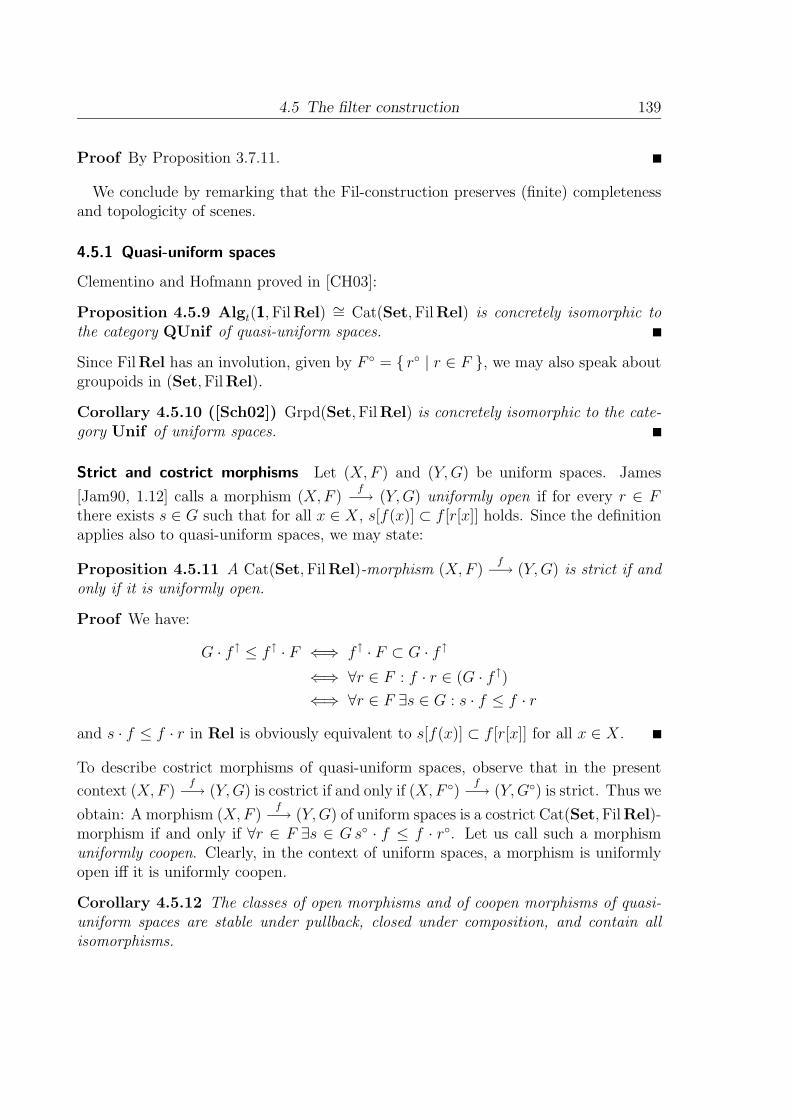
4.5 The filter construction 139
Proof By Proposition 3.7.11.
We conclude by remarking that the Fil-construction preserves (finite) completenessand topologicity of scenes.
4.5.1 Quasi-uniform spaces
Clementino and Hofmann proved in [CH03]:
Proposition 4.5.9 Algt(1, FilRel) ∼= Cat(Set, FilRel) is concretely isomorphic tothe category QUnif of quasi-uniform spaces.
Since FilRel has an involution, given by F ◦ = { r◦ | r ∈ F }, we may also speak aboutgroupoids in (Set, FilRel).
Corollary 4.5.10 ([Sch02]) Grpd(Set, FilRel) is concretely isomorphic to the cate-gory Unif of uniform spaces.
Strict and costrict morphisms Let (X,F ) and (Y,G) be uniform spaces. James
[Jam90, 1.12] calls a morphism (X,F )f−→ (Y,G) uniformly open if for every r ∈ F
there exists s ∈ G such that for all x ∈ X, s[f(x)] ⊂ f [r[x]] holds. Since the definitionapplies also to quasi-uniform spaces, we may state:
Proposition 4.5.11 A Cat(Set, FilRel)-morphism (X,F )f−→ (Y,G) is strict if and
only if it is uniformly open.
Proof We have:
G · f ↑ ≤ f ↑ · F ⇐⇒ f ↑ · F ⊂ G · f ↑
⇐⇒ ∀r ∈ F : f · r ∈ (G · f ↑)
⇐⇒ ∀r ∈ F ∃s ∈ G : s · f ≤ f · r
and s · f ≤ f · r in Rel is obviously equivalent to s[f(x)] ⊂ f [r[x]] for all x ∈ X.
To describe costrict morphisms of quasi-uniform spaces, observe that in the present
context (X,F )f−→ (Y,G) is costrict if and only if (X,F ◦)
f−→ (Y,G◦) is strict. Thus we
obtain: A morphism (X,F )f−→ (Y,G) of uniform spaces is a costrict Cat(Set, FilRel)-
morphism if and only if ∀r ∈ F ∃s ∈ Gs◦ · f ≤ f · r◦. Let us call such a morphismuniformly coopen. Clearly, in the context of uniform spaces, a morphism is uniformlyopen iff it is uniformly coopen.
Corollary 4.5.12 The classes of open morphisms and of coopen morphisms of quasi-uniform spaces are stable under pullback, closed under composition, and contain allisomorphisms.

140 4 Further examples
Proof The (co-)Frobenius law as well as the (BC)-property hold in (FilRel,Set).
Proposition 4.5.13 Every surjective open and every surjective coopen morphism ofquasi-uniform spaces is an effective descent morphism in QUnif .
Proof Clearly the reasoning of Section 3.6.3 applies.
Strict diagonals For a morphism Xf−→ Y in a finitely complete category, write
Ker f for the following pullback:
Ker ff1
��
f0
��
X
f
��
Xf
�� Y
and define the diagonal δf : X −→ Ker f of f by f1 · δf = 1X = f0 · δf .
Proposition 4.5.14 Let (X,F )f−→ (X,G) by a morphism of uniform spaces. Then
the diagonal δf is uniformly open if and only if f is transverse to F in the sense of[Jam90], that is, there exists r ∈ F such that 1X = r ∩ { (x, x′) ∈ X2 | f(x) = f(x′) }.
Proof We will first give a description of the uniform space Ker f . First observe thatwe may assume Ker f to be canonically constructed, that is, the underlying set of Ker fis the set in the statement of the proposition.
Let us denote the uniform structure on Ker f by H. From the construction of initialstructures, we see that for s ⊂ (Ker f)2 we have, by Remark 4.5.1 and the fact that Fis a filter,
s ∈ H ⇐⇒ ∃r ∈ F : f ◦0 · r · f0 ∩ f ◦
1 · r · f1 ⊂ s.
Suppose now that δf is open. Since (X × X) ∈ F , we obtain s ∈ H with s[δf (x)] ⊂δf [(X ×X)[x]] = 1X for all x ∈ X, that is, whenever (x, x) s (x0, x1), then x0 = x1. Byconstruction of H, there exists some r ∈ F with f ◦
0 · r · f0 ∩ f ◦1 · r · f1 ⊂ s. We claim
that this r satisfies r ∩ Ker f = 1X . Indeed, whenever we have x0 (r ∩ Ker f) x1, thensince x0 r x0 by 1X ⊂ r, we obtain
(x0, x0) (f ◦0 · r · f0) (x0, x1) and (x0, x0) (f ◦
1 · r · f1) (x0, x1),
thus (x0, x0) s (x0, x1), and hence x0 = x1.Suppose that f is transverse to F , that is, there exists r0 ∈ F with r0 ∩Ker f = 1X .
For any r ∈ F , set r1 = r ∩ r0 ∈ F . We clearly have r1 ∩ Ker f = 1X . Defines = f ◦
0 · r1 · f0 ∩ f ◦1 · r1 · f1. We claim that s[δf (x)] ⊂ δf [r[x]] holds for all x ∈ X. Fix
x ∈ X, and take any (x0, x1) ∈ Ker f with (x, x) s (x0, x1), thus, x r1 x0 and x r1 x1.Since r1 ∈ F , and (X,F ) is an uniform spaces, we obtain x0 r1 x1. Thus, x0 = x1 sincer1 ∩Ker f = 1X . Moreover, (x, x0) ∈ r1 ⊂ r gives (x0, x1) ∈ δf [r[x]].
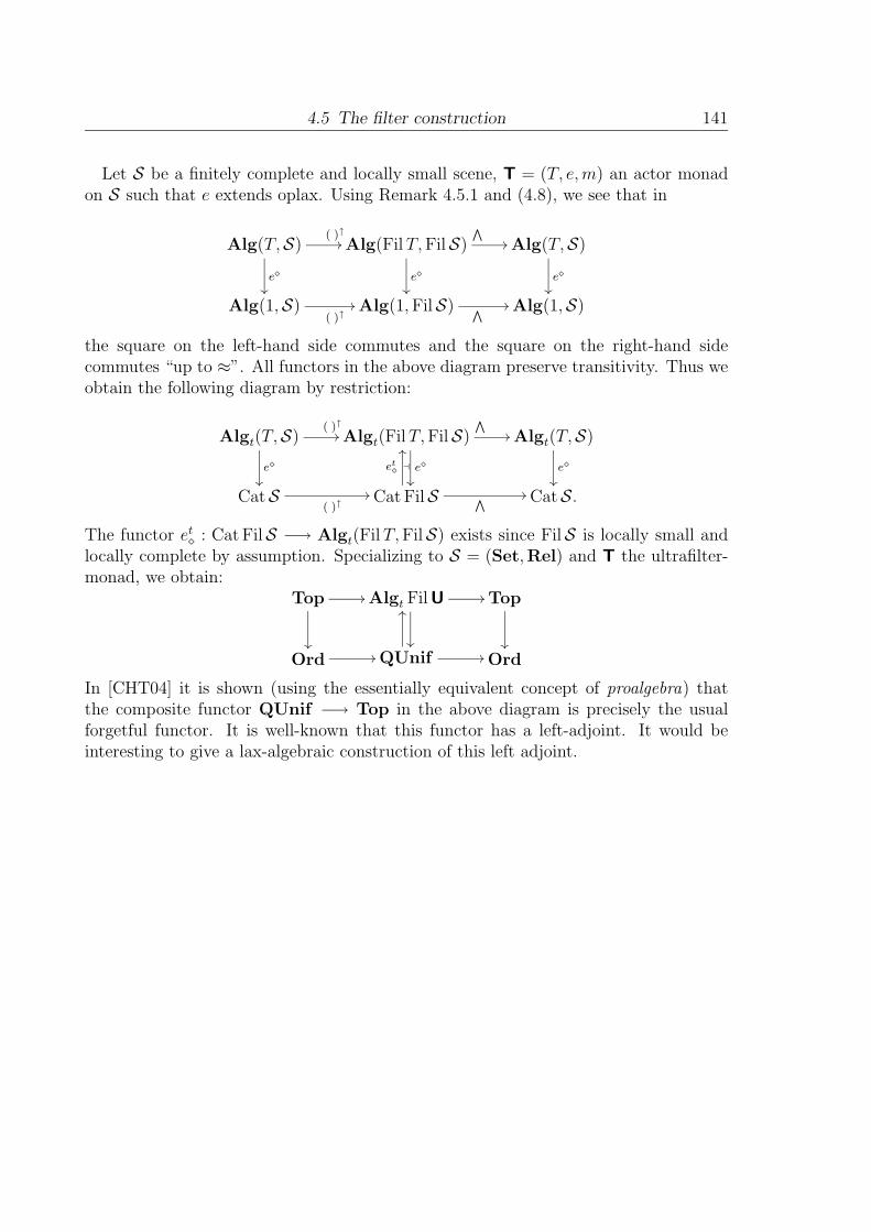
4.5 The filter construction 141
Let S be a finitely complete and locally small scene, T = (T, e,m) an actor monadon S such that e extends oplax. Using Remark 4.5.1 and (4.8), we see that in
Alg(T,S)
e
��
( )↑�� Alg(Fil T, FilS)
e
��
V
�� Alg(T,S)
e
��
Alg(1,S)( )↑
�� Alg(1, FilS) V
�� Alg(1,S)
the square on the left-hand side commutes and the square on the right-hand sidecommutes “up to ≈”. All functors in the above diagram preserve transitivity. Thus weobtain the following diagram by restriction:
Algt(T,S)
e
��
( )↑�� Algt(Fil T, FilS)
� e
��
V
�� Algt(T,S)
e
��
CatS( )↑
�� Cat FilS
et
��
V
�� CatS.
The functor et : Cat FilS −→ Algt(Fil T, FilS) exists since FilS is locally small and
locally complete by assumption. Specializing to S = (Set,Rel) and T the ultrafilter-monad, we obtain:
Top
��
�� Algt FilU
��
�� Top
��
Ord �� QUnif
��
�� Ord
In [CHT04] it is shown (using the essentially equivalent concept of proalgebra) thatthe composite functor QUnif −→ Top in the above diagram is precisely the usualforgetful functor. It is well-known that this functor has a left-adjoint. It would beinteresting to give a lax-algebraic construction of this left adjoint.

142 4 Further examples

5 Partial morphisms
In this chapter we are going to study whether partial morphism in categories of laxalgebras are representable. We will give some applications to T0-objects and the expo-nentiability of monomorphisms in categories of lax algebras.
5.1 Generalities
First we will review the notion of partial morphism; we follow quite closely [AHS04,Section 28]. Let X be a category,M be a class of X-morphisms. AM-partial morphismfrom A to B is a span
Am←− •
f−→ B (5.1)
with m ∈M.We say that B
ηB−→ B+ represents (or is a representer for)M-partial morphisms intoB provided that
1. ηB ∈M,
2. for every morphism Af−→ B+ there exists a pullback
Pm ��
f ′
��
A
f
��
B ηB
�� B+
with m ∈M, and
3. for each M-partial morphism Am←− X
f−→ B there exists a unique A
f−→ B+
such that
Xm ��
f
��
A
f��
B ηB
�� B+
is a pullback.
We say that X has representable M-partial morphisms if for every B ∈ X there existsB
ηB−→ B+ which represents M-partial morphisms into B.
Remark 5.1.1 If X has representableM-partial morphisms then we obtain a pointedendofunctor (( )+, η). Moreover, η is cartesian.
143
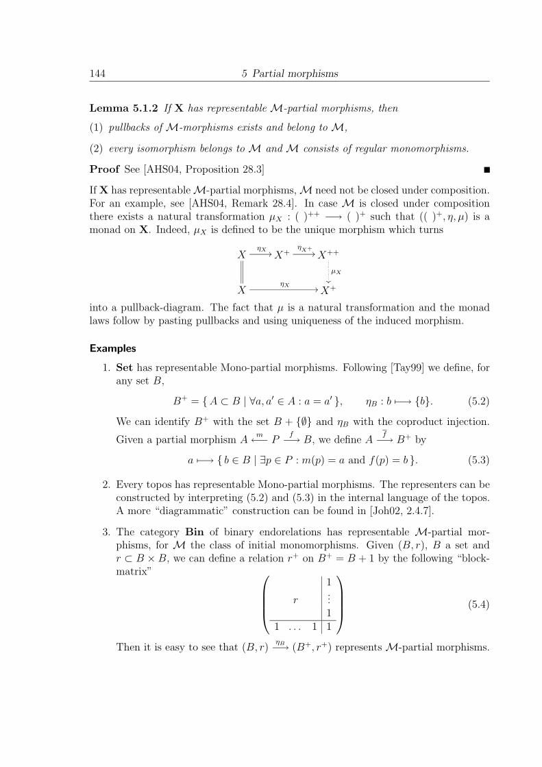
144 5 Partial morphisms
Lemma 5.1.2 If X has representable M-partial morphisms, then
(1) pullbacks of M-morphisms exists and belong to M,
(2) every isomorphism belongs to M and M consists of regular monomorphisms.
Proof See [AHS04, Proposition 28.3]
If X has representableM-partial morphisms,M need not be closed under composition.For an example, see [AHS04, Remark 28.4]. In case M is closed under compositionthere exists a natural transformation μX : ( )++ −→ ( )+ such that (( )+, η, μ) is amonad on X. Indeed, μX is defined to be the unique morphism which turns
XηX �� X+
ηX+
�� X++
μX
��
XηX �� X+
into a pullback-diagram. The fact that μ is a natural transformation and the monadlaws follow by pasting pullbacks and using uniqueness of the induced morphism.
Examples
1. Set has representable Mono-partial morphisms. Following [Tay99] we define, forany set B,
B+ = {A ⊂ B | ∀a, a′ ∈ A : a = a′ }, ηB : b �−→ {b}. (5.2)
We can identify B+ with the set B + {∅} and ηB with the coproduct injection.
Given a partial morphism Am←− P
f−→ B, we define A
f−→ B+ by
a �−→ { b ∈ B | ∃p ∈ P : m(p) = a and f(p) = b }. (5.3)
2. Every topos has representable Mono-partial morphisms. The representers can beconstructed by interpreting (5.2) and (5.3) in the internal language of the topos.A more “diagrammatic” construction can be found in [Joh02, 2.4.7].
3. The category Bin of binary endorelations has representable M-partial mor-phisms, for M the class of initial monomorphisms. Given (B, r), B a set andr ⊂ B × B, we can define a relation r+ on B+ = B + 1 by the following “block-matrix” ⎛⎜⎜⎜⎝
1
r...1
1 . . . 1 1
⎞⎟⎟⎟⎠ (5.4)
Then it is easy to see that (B, r)ηB−→ (B+, r+) represents M-partial morphisms.

5.2 Representing initial morphisms 145
Using the last example, we can explain out general strategy for constructing represen-ters in categories of lax algebras: ηB defines a function
η B = η∗
B · ( ) · ηB : Rel(B+, B+) −→ Rel(B,B), (5.5)
and r+ is just the maximal element of Rel(B+, B+) such that η B(r+) ≤ r. That is,
the assignment r �−→ r+ determines a right-adjoint of η B. This observation allows us
to give a purely categorical proof of the existence of representers for suitable classes ofmorphisms in categories of lax algebras.
5.2 Representing initial morphisms
Proposition 5.2.1 Let P : X −→ B be a faithful fibration and let Xf−→ Z
g←− Y be
X-morphisms with f initial. If
Dp
��
q
��
PY
Pg
��
PXPf
�� PZ
is a pullback in B, then the pullback of f along g exists in X and is initial.
If P is a faithful fibration and M is a class of B-morphisms we write, as before,
MI := { f ∈ X | f is initial and Pf ∈M}.
Proposition 5.2.2 Let P : X −→ B be a faithful fibration such that P has a rightand a left adjoint, that is, (X, P ) has discrete and indiscrete objects.
If M is a class of B-morphisms such that MI-partial morphisms are representablein X, then M-partial morphisms are representable in B.
Moreover, P preserves representers if and only if MI-subobjects of discrete objectsare discrete.
Proof The proof of Proposition 28.12 in [AHS04] applies.
Observe that MI-subalgebras of discrete algebras in Alg T are discrete provided com-position preserves the bottom-element, and MI-subalgebras of discrete algebras inAlgrT, AlguT, and AlgtT are discrete if T sends M-morphisms into injections.
Since most categories of lax algebras of interest satisfy the additional requirementsof the above proposition, we will only study the problem of lifting a given M-partialmorphism representer.

146 5 Partial morphisms
Blanket assumptions We fix a scene S which satisfies the Beck–Chevalley propertyand a class M ⊂ morS such that (( )+, η) represents M-partial morphisms in S.Moreover, we fix an actor T on S such that T has the (BC)-property with respectto M. These assumptions are fulfilled, for example, for S = (Set, MatV) and any(extension of a) taut Set-functor T .
Lemma 5.2.3 The blanket assumptions imply the following statements:
(1) every M-morphism is an injection;
(2) every T -image of a M-morphism is an injection.
Proof Every (Am−→ X) ∈M is a monomorphism, hence
A A
m
��
A m�� X
is a pullback, and Beck–Chevalley implies m∗ ·m ≈ 1A and Tm∗ · Tm ≈ 1TA.
We aim at the following theorem:
Theorem 5.2.4 The following statements are equivalent for an S-object B:
(1) ψ = η B : D(T (B+), B+) −→ D(TB,B), a �−→ η∗
B · a · TηB has a right adjoint φ;
(2) for every lax algebra (B, b) there is a lift (B+, b+) of B+ such that (B, b)ηB−→
(B+, b+) represents MI-partial morphisms into (B, b).
In this case b+ = φ(b).
Some observations: ψ always has a fully-faithful left adjoint ηB , given by c �−→ ηB · c ·Tη∗
B. Hence, by Lemma 1.2.11, any right adjoint φ which might exist is forced to befully-faithful.
Proof (2) implies (1): Define φ(b) = b+. First observe that φ is monotone. Indeed, if
b ≤ c, then (B, b)1B−→ (B, c) is a morphism and the upper-left corner in
(B, b)
1B
��
ηB �� (B+, b+)
f
��
(B, c) ηB
�� (B+, c+)
(5.6)
is a MI-partial morphism into (B, c), hence there exists a unique f such that (5.6) isa pullback. Clearly, f = 1B, hence b+ ≤ c+.

5.2 Representing initial morphisms 147
Initiality of ηB gives ψ · φ ≈ 1. It remains to show 1 ≤ φ ·ψ, i.e. a ≤ (ψa)+ for everya ∈ D(TB+, B+). Consider
(B,ψa)ηB �� (B+, a)
f
��
(B,ψa) ηB
�� (B+, (ψa)+).
The upper-left corner is a MI-partial morphism by definition of ψa, hence there is aunique f as shown such that the diagram is a pullback, clearly f = 1B+ and the claimfollows.
Initiality of ηB follows from ψ · φ ≈ 1.
(1) implies (2): ψ ·φ ≈ 1 is equivalent to the initiality of (B, b)ηB−→ (B+, φ(b)). Suppose
(B, b)f←− (Y, a)
m−→ (Z, c) is an MI-partial morphism. Then there exists a unique f
such that
Ym ��
f
��
Z
f��
B ηB
�� B+
(5.7)
is a pullback in S. Since the above as well as its T -image is a (BC)-square,
ψ(f · c · Tf∗) ≈ η∗
B · f · c · Tf∗· TηB ≈ f ·m∗ · c · Tm · Tf∗ ≈ f · a · Tf ∗ ≤ b
holds, which, by ψ −� φ implies that (Z, c)f−→ (B+, b+) is a morphism. Since m is
initial, the above diagram becomes a pullback in Alg T .
Representations in categories of reflexive and unitary algebras
Proposition 5.2.5 (B, b) is reflexive if and only if (B+, b+) is reflexive.
Proof Suppose (B, b) is reflexive. It suffices to show ψ(e∗B+) ≤ b, which holds sinceη∗
B · e∗B+ · TηB ≈ e∗B · Tη∗
B · TηB ≈ e∗B ≤ b.
The converse follows from the initiality of (B, b)ηB−→ (B+, b+).
Proposition 5.2.6 If m has the (BC)-property with respect to M, then (B, b) is uni-tary if and only if (B+, b+) is unitary.
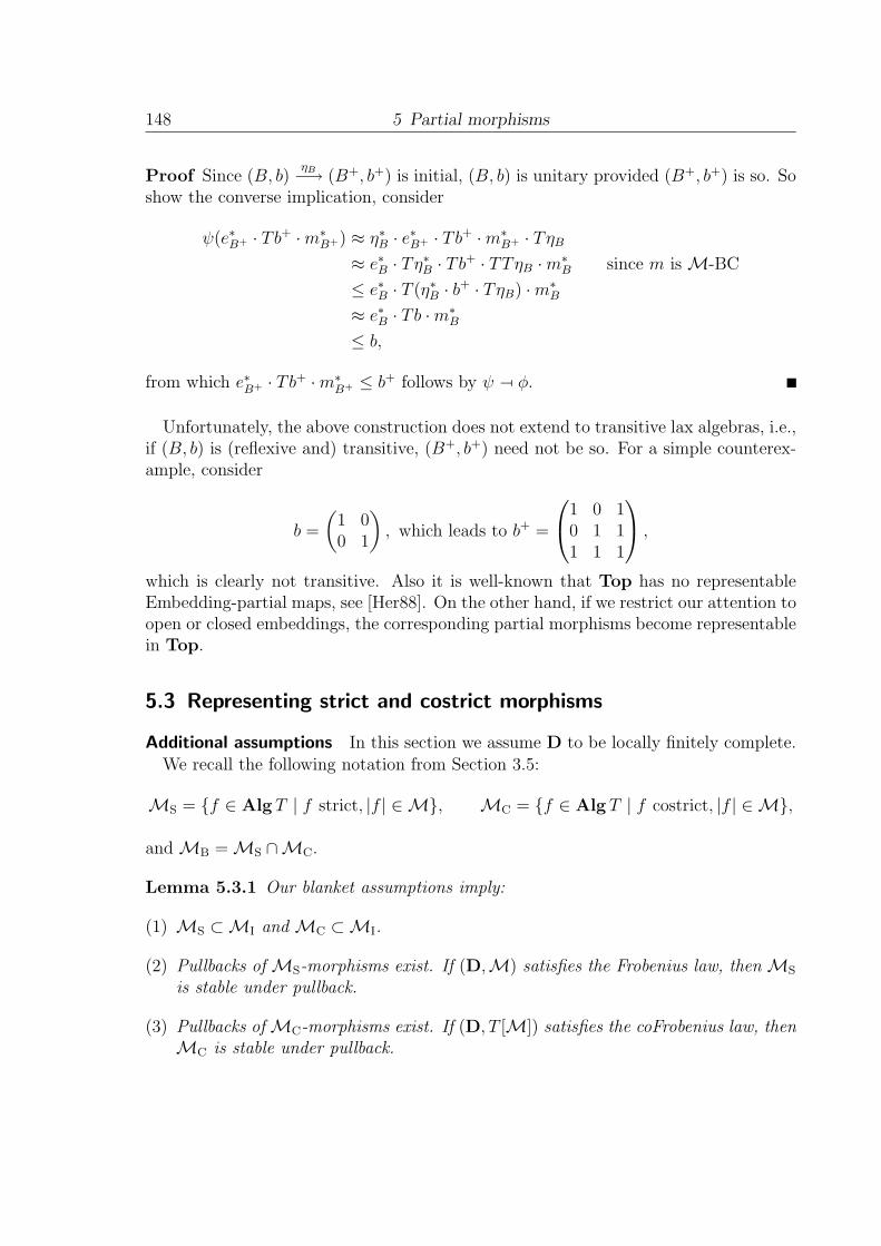
148 5 Partial morphisms
Proof Since (B, b)ηB−→ (B+, b+) is initial, (B, b) is unitary provided (B+, b+) is so. So
show the converse implication, consider
ψ(e∗B+ · Tb+ ·m∗B+) ≈ η∗
B · e∗B+ · Tb+ ·m∗
B+ · TηB
≈ e∗B · Tη∗B · Tb+ · TTηB ·m
∗B since m is M-BC
≤ e∗B · T (η∗B · b
+ · TηB) ·m∗B
≈ e∗B · Tb ·m∗B
≤ b,
from which e∗B+ · Tb+ ·m∗B+ ≤ b+ follows by ψ − � φ.
Unfortunately, the above construction does not extend to transitive lax algebras, i.e.,if (B, b) is (reflexive and) transitive, (B+, b+) need not be so. For a simple counterex-ample, consider
b =
(1 00 1
), which leads to b+ =
⎛⎝1 0 10 1 11 1 1
⎞⎠ ,
which is clearly not transitive. Also it is well-known that Top has no representableEmbedding-partial maps, see [Her88]. On the other hand, if we restrict our attention toopen or closed embeddings, the corresponding partial morphisms become representablein Top.
5.3 Representing strict and costrict morphisms
Additional assumptions In this section we assume D to be locally finitely complete.We recall the following notation from Section 3.5:
MS = {f ∈ Alg T | f strict, |f | ∈ M}, MC = {f ∈ Alg T | f costrict, |f | ∈ M},
and MB = MS ∩MC.
Lemma 5.3.1 Our blanket assumptions imply:
(1) MS ⊂MI and MC ⊂MI.
(2) Pullbacks of MS-morphisms exist. If (D,M) satisfies the Frobenius law, then MS
is stable under pullback.
(3) Pullbacks of MC-morphisms exist. If (D, T [M]) satisfies the coFrobenius law, thenMC is stable under pullback.
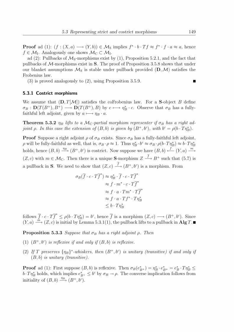
5.3 Representing strict and costrict morphisms 149
Proof ad (1): (f : (X, a) −→ (Y, b)) ∈ MS implies f ∗ · b · Tf ≈ f ∗ · f · a ≈ a, hencef ∈MI. Analogously one shows MC ⊂MI.
ad (2): Pullbacks ofMS-morphisms exist by (1), Proposition 5.2.1, and the fact thatpullbacks of M-morphisms exist in S. The proof of Proposition 3.5.8 shows that underour blanket assumptions MS is stable under pullback provided (D,M) satisfies theFrobenius law.
(3) is proved analogously to (2), using Proposition 3.5.9.
5.3.1 Costrict morphisms
We assume that (D, T [M]) satisfies the coFrobenius law. For a S-object B defineσB : D(T (B+), B+) −→ D(T (B+), B) by c �−→ η∗
B · c. Observe that σB has a fully-faithful left adjoint, given by a �−→ ηB · a.
Theorem 5.3.2 ηB lifts to a MC-partial morphism representer if σB has a right ad-joint ρ. In this case the extension of (B, b) is given by (B+, bc), with bc = ρ(b · Tη∗
B).
Proof Suppose a right adjoint ρ of σB exists. Since σB has a fully-faithful left adjoint,ρ will be fully-faithful as well, that is, σB ·ρ ≈ 1. Thus η∗
B · bc ≈ σB ·ρ(b ·Tη∗
B) ≈ b ·Tη∗B
holds, hence (B, b)ηB−→ (B+, bc) is costrict. Now suppose we have (B, b)
f←− (Y, a)
m−→
(Z, c) with m ∈MC. Then there is a unique S-morphism Zf−→ B+ such that (5.7) is
a pullback in S. We need to show that (Z, c)f−→ (B+, bc) is a morphism. From
σB(f · c · Tf∗) ≈ η∗
B · f · c · Tf∗
≈ f ·m∗ · c · Tf∗
≈ f · a · Tm∗ · Tf∗
≈ f · a · Tf∗ · Tη∗B
≤ b · Tη∗B
follows f · c · Tf∗≤ ρ(b · Tη∗
B) = bc, hence f is a morphism (Z, c) −→ (B+, bc). Since(Y, a)
m−→ (Z, c) is initial by Lemma 5.3.1(1), the pullback lifts to a pullback in Alg T .
Proposition 5.3.3 Suppose that σB has a right adjoint ρ. Then
(1) (B+, bc) is reflexive if and only if (B, b) is reflexive.
(2) If T preserves {ηB}∗-whiskers, then (B+, bc) is unitary (transitive) if and only if
(B, b) is unitary (transitive).
Proof ad (1): First suppose (B, b) is reflexive. Then σB(e∗B+) = η∗B · e
∗B+ = e∗B ·Tη∗
B ≤b ·Tη∗
B holds, which implies e∗B+ ≤ bc by σB − � ρ. The converse implication follows from
initiality of (B, b)ηB−→ (B+, bc).

150 5 Partial morphisms
ad (2): Strictness of T implies
Tη∗B ·Tbc ·m∗
B+ ≈ T (η∗B ·b
c) ·m∗B+ ≈ T (b ·Tη∗
B) ·m∗B+ ≈ Tb ·TTη∗
B ·m∗B+ ≈ Tb ·m∗
B ·Tη∗B.
Suppose (B, b) is unitary. Using the above equation, we obtain
σB(e∗B+ · Tbc ·m∗B+) ≈ η∗
B · e∗B+ · Tbc ·m∗
B+
≈ e∗B · Tη∗B · Tbc ·m∗
B+
≈ e∗B · Tb ·m∗B · Tη∗
B
≤ b · Tη∗B.
In case (B, b) is transitive, we obtain:
σB(bc · Tbc ·m∗B+) ≈ η∗
B · bc · Tbc ·m∗
B+
≈ b · Tη∗B · Tbc ·m∗
B+
≈ b · Tb ·m∗B · Tη∗
B
b · Tη∗B.
Therefore, unitarity (transitivity) of (B, b) implies unitarity (transitivity) of (B+, bc)
by σB −� ρ. The converse implications follow from initiality of (B, b)ηB−→ (B+, bc).
5.3.2 Strict morphisms
We assume that (D,M) satisfies the Frobenius law.Let B be an S-object and define τB : D(T (B+), B+) −→ D(TB,B+) by c �−→ c·TηB.
Observe that τB has a fully-faithful left adjoint, given by a �−→ a · Tη∗B.
Theorem 5.3.4 ηB lifts to aMS-partial morphism representer if τB has a right adjointυ. In this case the extension of (B, b) is given by (B+, bs) with bs = υ(ηB · b).
Proof Any right adjoint υ will be fully-faithful, that is, will satisfy τB · υ ≈ 1.(B, b)
ηB−→ (B+, b+) is strict since bs · TηB ≈ τB(υ(ηB · b)) ≈ ηB · b. Now suppose we
have (B, b)f←− (Y, a)
m−→ (Z, c) with m ∈ MS. Then there is a unique S-morphism
Zf−→ B+ such that (5.7) is a pullback in S. We need to show that (Z, c)
f−→ (B+, bs)
is a morphism. From
τB(f · c · Tf∗) ≈ f · c · Tf
∗· TηB
≈ f · c · Tm · Tf∗
≈ f ·m · a · Tf∗
≈ ηB · f · a · Tf ∗
≤ ηB · b
follows f · c · Tf∗≤ υ(ηB · b) = bs, thus (Z, c)
f−→ (B+, bs) is a morphism. Since m is
initial, the pullback (5.7) lifts to a pullback in Alg T .

5.4 Examples 151
Proposition 5.3.5 Suppose that τB has a right adjoint υ. Then
(1) If e has the (BC)-property with respect to M, then (B+, bs) is reflexive if and onlyif (B, b) is reflexive.
(2) If T preserves {ηB}-whiskers and e, m have the (BC)-property with respect to M,then (B+, bs) is transitive if and only if (B, b) is transitive.
(3) If T preserves {ηB}-whiskers, and m has the (BC)-property with respect to M,then (B+, bs) is transitive if and only if (B, b) is transitive.
Proof Suppose (B, b) is reflexive. Then τB(e∗B+) = e∗B+ · TηB ≈ ηB · e∗B ≤ ηB · b holds,
which, using τB −� υ, implies reflexivity of (B+, bs).Strictness of T and the fact that m has the (BC)-property with respect to M imply
Tbs ·m∗B+ ·TηB ≈ Tbs ·TTηB ·m
∗B ≈ T (bs ·TηB) ·m∗
B ≈ T (ηB · b) ·m∗B ≈ TηB ·Tb ·m∗
B.
Suppose (B, b) is unitary. We obtain:
τB(e∗B+ · Tbs ·m∗B+) ≈ e∗B+ · Tbs ·m∗
B+ · TηB
≈ e∗B+ · TηB · Tb ·m∗B
≈ ηB · e∗B · Tb ·m∗
B
≤ ηB · b.
In case (B, b) is transitive, we obtain:
τB(bs · Tbs ·m∗B+) ≈ bs · Tbs ·m∗
B+ · TηB
≈ bs · TηB · Tb ·m∗B
≈ ηB · b · Tb ·m∗B
≤ ηB · b.
Hence, unitarity (transitivity) or (B+, bs) follows from unitarity (transitivity) of (B, b)
by τB −� υ. The converse implications follow by initiality of (B, b)ηB−→ (B+, bs).
5.4 Examples
Over MatV Let us first consider the case S = (Set, MatV) for an arbitrary quantaleV. Let M denote the class of injective functions. A functor T : Set −→ Set mapsinverse images to (BC)-squares if and only if T is taut. A natural transformation hasthe (BC)-property with respect to M if and only if it is taut. Finally, MatV hasdivision since it is a quantaloid, thus all the required right adjoints exist. Thus wehave:

152 5 Partial morphisms
Proposition 5.4.1 For any actor T on S = (Set, MatV) with T : Set −→ Set taut,partial morphisms are representable in Alg T and the forgetful functor Alg T −→ Setpreserves representations.
If T = (T, e,m) is a monadic actor on S with T taut, then also AlgrT has concretelyrepresentable partial morphisms. If m is a taut transformation, then also AlguT hasconcretely representable partial morphisms.
Since in the present context, (MatV,M) satisfies both the Frobenius and the coFrobe-nius law, and for any taut Set-functor its extension to MatV preserves {Mono}- and{Mono}∗-whiskers, we also have:
Proposition 5.4.2 For any monadic actor T on (Set, MatV) with T taut, Alg T ,AlgrT, AlguT, and AlgtT have concretely representable costrict-embedding partialmorphisms.
In case (T, e,m) is a taut Set-monad, Alg T , AlgrT, AlguT, and AlgtT haveconcretely representable strict-embedding partial morphisms.
Thus in particular, PsTop, PrTop, PsAp, PrAp, Bin, RBin have concretelyrepresentable partial morphisms. Top and Ap have concrete representations for open-and closed-embedding partial morphisms. Ord has concrete representations for up-and down-closed embedding-partial morphisms.
The same reasoning applies to Clos (recall that the extension of U to Dist is a 2-functor). Thus we obtain that closed-embedding partial morphisms are representablein Clos.
All the above-mentioned representations are done by one-point extensions.
Over RelC Proposition 5.4.2 remains true in for any scene of the form (C, RelC),provided C is a logos. To wit:
Proposition 5.4.3 Let C be a logos, M ⊂ morC a class of morphisms such thatC has representable M-partial morphisms, T a taut functor C −→ C. Alg T hasrepresentable MI-partial morphisms and the forgetful functor preserves them.
In case T = (T, e,m) is a monad on C with T taut, also AlgrT has concretelyrepresentable MI-partial morphism. Furthermore, Alg T , AlgrT, AlguT, and AlgtThave concretely representable MC-partial morphisms.
If moreover m is taut, then also AlgrT has concretely representable MI-partial mor-phisms.
If T is a taut monad on C, then Alg T , AlgrT, AlguT, and AlgtT have concretelyrepresentable MS-partial morphisms.
5.5 Some applications
We are now giving some applications of the results in this Chapter. To make thediscussion more understandable, we leave out some (easily established) technical details.

5.5 Some applications 153
5.5.1 Subobject classifier and T0-objects
Recall that, for a classM of (mono-)morphisms in a category X with a terminal object
1, a M-subject classifier is a morphism 1t−→ Ω such that for every A
m−→ X in M,
there exists a unique morphism XχA−→ Ω such that
Am ��
��
X
χA
��
1t
�� Ω
is a pullback. In case M-partial morphisms are representable in X, clearly 1η1−→ 1+
is M-subobject classifier. In general, representability of M-partial morphisms is astronger condition than the existence of M-subobject classifiers, cf. Lemma 5.5.3.
In particular, Top has a subobject classifier 1t−→ S for open-embeddings. Here S
is the Sierpinski-space and t “is” the “open point” of S.Of course, this definition can now be mimicked in every category of lax algebras with
representable MC-partial morphisms (M a suitable class of monomorphisms), leadingto a notion of Sierpinski-object for the class of lax algebras under consideration.
Mindful of the fact that a topological space is T0 if and only if it is a subspace of apower of S, we can now define a lax algebra to be T0 if it lies in the full subcategorycogenerated by the respective Sierpinski-object.
In fact this has been done by Manes [Man02] for reflexive and transitive lax algebrasover the scene (Set,Rel) for an actor defined by a taut Set-functor. He uses an explicitconstruction of the Sierpinski-object.
We end up with the following examples:
• T0-objects in Top ∼= AlgtT are precisely the T0-topological spaces;
• T0-objects in Ord ∼= Algt1 are precisely the anti-symmetric ordered sets.
5.5.2 Exponentiability
We will now apply the results obtained so far to give examples of exponentiable mor-phisms in various categories of lax algebras.
Let X denote a finitely complete category. A morphism f : X −→ Y in X is calledexponentiable if ( )× f : X/Y −→ X/Y has a right adjoint. We note two well-knownresults on exponentiable morphisms. For proofs we refer to [Nie82].
Lemma 5.5.1 The following statements are equivalent for f : X −→ Y in X:
(1) f is exponentiable;
(2) the pullback functor f ∗ : X/Y −→ X/X has a right adjoint.
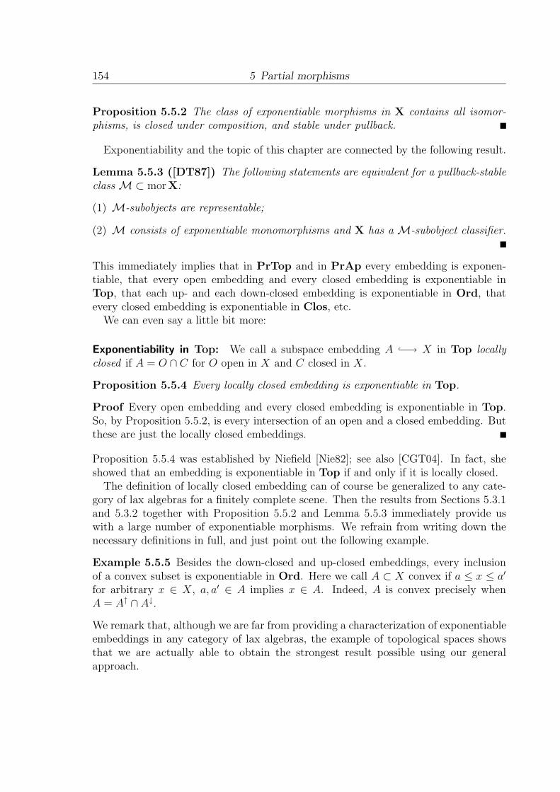
154 5 Partial morphisms
Proposition 5.5.2 The class of exponentiable morphisms in X contains all isomor-phisms, is closed under composition, and stable under pullback.
Exponentiability and the topic of this chapter are connected by the following result.
Lemma 5.5.3 ([DT87]) The following statements are equivalent for a pullback-stableclass M⊂ morX:
(1) M-subobjects are representable;
(2) M consists of exponentiable monomorphisms and X has a M-subobject classifier.
This immediately implies that in PrTop and in PrAp every embedding is exponen-tiable, that every open embedding and every closed embedding is exponentiable inTop, that each up- and each down-closed embedding is exponentiable in Ord, thatevery closed embedding is exponentiable in Clos, etc.
We can even say a little bit more:
Exponentiability in Top: We call a subspace embedding A ↪−→ X in Top locallyclosed if A = O ∩ C for O open in X and C closed in X.
Proposition 5.5.4 Every locally closed embedding is exponentiable in Top.
Proof Every open embedding and every closed embedding is exponentiable in Top.So, by Proposition 5.5.2, is every intersection of an open and a closed embedding. Butthese are just the locally closed embeddings.
Proposition 5.5.4 was established by Niefield [Nie82]; see also [CGT04]. In fact, sheshowed that an embedding is exponentiable in Top if and only if it is locally closed.
The definition of locally closed embedding can of course be generalized to any cate-gory of lax algebras for a finitely complete scene. Then the results from Sections 5.3.1and 5.3.2 together with Proposition 5.5.2 and Lemma 5.5.3 immediately provide uswith a large number of exponentiable morphisms. We refrain from writing down thenecessary definitions in full, and just point out the following example.
Example 5.5.5 Besides the down-closed and up-closed embeddings, every inclusionof a convex subset is exponentiable in Ord. Here we call A ⊂ X convex if a ≤ x ≤ a′
for arbitrary x ∈ X, a, a′ ∈ A implies x ∈ A. Indeed, A is convex precisely whenA = A↑ ∩ A↓.
We remark that, although we are far from providing a characterization of exponentiableembeddings in any category of lax algebras, the example of topological spaces showsthat we are actually able to obtain the strongest result possible using our generalapproach.
6 More on limits and colimits
6.1 Coproducts
The material presented in this section is mostly an extension of [MST06].In this section, we will fix a scene S = (S,C,D) and say that the (finite) basic
assumptions are satisfied provided
(1) D is locally small, has locally (finite) suprema, and these are preserved by compo-sition,
(2) S has (finite) coproducts, and the embedding S( )∗·E−→ D sends them to biproducts.
We write C for the class of all coproduct-injections in S.Examples of scenes which satisfy the (finite) basic are:
• (Set, MatV) for any quantale V.
• Let C be a well-powered regular category. (C, RelC) satisfies the (finite) basicassumptions provided C has (finite) coproducts and is (finitely) extensive; see[FS90].
• If S satisfies the (finite) basic assumption, so does Dist(S). This is shown inLemma 1.6.5 and Proposition 1.6.10.
• O(V) = (Set,Ord, OrdMat(V)) satisfies the basic assumptions. To see this,observe that the proof of Proposition 1.6.10 shows that OrdMat(V) is closedunder biproducts in Dist(Set, MatV).
6.1.1 Coproducts in categories of lax algebras
Since Alg T| |−→ S is a fibering Alg T has (finite) concrete coproducts precisely when S
has (finite) coproducts and the fibers of | | have (finite) coproducts, that is, D(TB,B)has (finite) suprema for all B ∈ S.
To study more refined properties of coproducts in Alg T , we will now assume that the(finite) basic assumptions are satisfied. In particular, the forgetful functor Alg T −→ Shas a left adjoint, and thus preserves all limits which exist in Alg T .
Proposition 6.1.1 AlgT has (finite) concrete coproducts. The following statements
are equivalent for a (finite) family (Xi, ai)I in Alg T and a coproduct (Xiti−→ X)I in
S:
155

156 6 More on limits and colimits
(1)((Xi, ai)
ti−→ (X, a))
Iis a coproduct in Alg T ;
(2) each (Xi, ai)ti−→ (X, a) is costrict.
Proof Existence and concreteness of coproducts follow from the above remarks. Sup-
pose((Xi, ai)
ti−→ (X, a))
Iis a coproduct in Alg T . By essential uniqueness of final
lifts, we have a ≈∨
I ti · ai · Tt∗i , and hence, using the fact that (Xiti−→ X)I is a
biproduct in D:
t∗j · a ≈ t∗j ·∨
ti · ai · Tt∗i ≈∨
t∗j · ti · ai · Tt∗i ≈ aj · Tt∗j ,
that is, each (Xj, aj)tj−→ (X, a) is costrict. On the other hand if each tj is costrict, we
obtain∨
ti · ai · Tt∗i ≈∨
ti · t∗i · a ≈ a, thus (X, a) is a final lax algebra with respect to
the coproduct sink, and hence a coproduct.
Since by the basic assumptions all coproduct-sinks are jointly covering in D, AlgrT isclosed under coproducts in Alg T by Proposition 3.4.20.
Proposition 6.1.2 Assume D to be a quantaloid and T to preserve C∗-whiskers. Given
a (finite) family (Xi, ai)I in AlgtT, a coproduct (Xiti−→ X)I in S, and a lax algebra
(X, a), the following statements are equivalent:
(1)((Xi, ai)
ti−→ (X, a))
Iis a coproduct in Alg T ;
(2) (X, a) is in AlgtT and((Xi, ai)
ti−→ (X, a))
Iis a coproduct in AlgtT;
(3) each ti : (Xi, ai) −→ (X, a) is costrict.
In particular, AlgtT is closed under coproducts in Alg T . The statements hold truewith AlguT in place of AlgtT.
Proof Observe first that under the conditions of the propositions, AlgtT is reflectivein Alg T , and thus coproducts are formed by applying the reflector to the coproductformed in Alg T .
[(1) ⇒ (2)]: Let (X, c) be a coproduct of the family (Xi, ai)I in AlgtT. By Proposition
3.5.10, each (Xi, ai)ti−→ (X, c) is open. Thus c ≈
∨ti · t
∗i · c ≈
∨ti · ai · Tt∗i ≈ a, that
is, c is just the final structure with respect to the coproduct embeddings, and thus thecoproduct of the family (Xi, ai)I in Alg T .
[(2) ⇒ (3)]: Proposition 3.5.10.
[(3) ⇒ (1)]: Proposition 6.1.1.
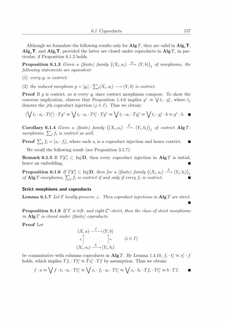
6.1 Coproducts 157
Although we formulate the following results only for Alg T , they are valid in AlgrT,AlguT, and AlgtT, provided the latter are closed under coproducts in Alg T , in par-ticular, if Proposition 6.1.2 holds.
Proposition 6.1.3 Given a (finite) family((Xi, ai)
gi−→ (Y, b))
Iof morphisms, the
following statements are equivalent:
(1) every gi is costrict;
(2) the induced morphism g = [gi] :∑
I(Xi, ai) −→ (Y, b) is costrict.
Proof If g is costrict, so is every gi since costrict morphisms compose. To show theconverse implication, observe that Proposition 1.4.6 implies g∗ ≈
∨ti · g
∗i , where tj
denotes the jth coproduct injection (j ∈ I). Thus we obtain:
(∨
ti · ai · Tt∗i ) · Tg∗ ≈∨
ti · ai · Tt∗i · Tg∗ ≈∨
ti · ai · Tg∗i ≈∨
ti · g∗i · b ≈ g∗ · b.
Corollary 6.1.4 Given a (finite) family((Xi, ai)
fi−→ (Yi, bi))
Iof costrict Alg T -
morphisms,∑
I fi is costrict as well.
Proof∑
I fi = [si · fi], where each si is a coproduct injection and hence costrict.
We recall the following result (see Proposition 3.5.7):
Remark 6.1.5 If T [C] ⊂ InjD, then every coproduct injection in Alg T is initial,hence an embedding.
Proposition 6.1.6 If T [C] ⊂ InjD, then for a (finite) family((Xi, ai)
fi−→ (Yi, bi))
I
of Alg T -morphisms,∑
I fi is costrict if and only if every fi is costrict.
Strict morphisms and coproducts
Lemma 6.1.7 Let T locally preserve ⊥. Then coproduct injections in Alg T are strict.
Proposition 6.1.8 If T is left- and right C∗-strict, then the class of strict morphismsin Alg T is closed under (finite) coproducts.
Proof Let
(X, a)f
�� (Y, b)
(Xi, ai)
ti
��
fi �� (Yi, bi)
si
��
(i ∈ I)
be commutative with columns coproducts in Alg T . By Lemma 1.4.10, fi · t∗i ≈ s∗i · f
holds, which implies Tfi · Tt∗i ≈ Ts∗i · Tf by assumption. Thus we obtain:
f · a ≈∨
f · ti · ai · Tt∗i ≈∨
si · fi · ai · Tt∗i ≈∨
si · bi · Tfi · Tt∗i ≈ b · Tf.
158 6 More on limits and colimits
Proposition 6.1.8 does not imply that given a family ((Xi, ai) −→ (Y, b)) of strictmorphisms, also the induced morphism
∐(Xi, ai) −→ (Y, b) is strict. In fact, this is
false. For a counterexample, consider the family({∗}
q−→ R
)q∈Q
in Top ∼= AlgtU
defined by q(∗) = q. Every q is a closed embedding, thus strict, but the inducedmorphism is not closed, thus not strict.
Proposition 6.1.9 Suppose we are given a diagram
(X, a)f
�� (Y, b)
(Xi, ai)
ti
��
fi
�����������(i ∈ I)
in Alg T such that the column is a coproduct and (Tti)I is jointly covering. Then f isstrict provided each fi is strict.
Clearly the above proposition applies in particular when T preserves I-fold coproducts.
6.1.2 The frame of a lax algebra
We assume the (infinite) basic assumptions, and additionally let (E ,M) be a splitable(with respect to S) factorization system on S such that S is M-wellpowered. As usual,we write MC for the class of costrict Alg T -morphisms whose underlying S-morphismis in M.
For each X in S, the ordered set SubMX of M-subobjects is a complete lattice.Indeed, given a (set-indexed) family (Ai
mi−→ X)I of M-subobjects, its supremumis given by the M-part of the (E ,M)-factorization of the induced morphism [mi] :∐
Ai −→ X.
Lemma 6.1.10 The set of costrictMI-subobjects of a lax algebra (X, a) is closed undersuprema in the complete lattice of MI-subobjects.
Proof We may use the construction as well as the notation from above. If each mi iscostrict, then also [mi] is costrict by Proposition 6.1.3. Now if we (E ,M)-factor [mi]as [mi] = m · e, e is a cover, and hence m is costrict as well, which proves our claim.
Now Proposition 3.5.9 gives closedness of MC-subobjects under binary intersections.Since each isomorphism is strict, we obtain:
Proposition 6.1.11 Suppose S to be finitely complete such that SubMX is a frame foreach S-object X, T has the (BC)-property with respect to M, and (D, T [M]) satisfiesthe coFrobenius law. Then the MC-subobjects of a lax algebra (X, a) form a subframeof SubMX, which we denote by T (X, a).
6.1 Coproducts 159
But Proposition 3.5.9 actually says more: for any Alg T -morphism (X, a)f−→ (Y, b),
the pullback-functor f−1 : SubMY −→ SubMX restricts to T (Y, b) −→ T (X, a). Hencewe have:
Proposition 6.1.12 Assume the conditions of Proposition 6.1.11 and, additionally,that for each f : X −→ Y in S, the pullback-functor f−1 : SubMY −→ SubMX is aframe morphism. Then T defines a functor Alg T −→ Loc into the category of locales.
Proof Recall that the category Loc of locales is the dual of the category of frames.Hence we can define T f to be f−1.
Over Set In case S = Set with E = Epi and M = Mono we can improve our resultssome more. Since SubMX is isomorphic to the powerset PX, we obtain T (X, a) asa subframe of PX, that is, as a topology on X. Thus T defines a concrete functorT ′ : Alg T −→ Top.
Proposition 6.1.13 T ′ : Alg T −→ Top preserves coproducts and sends costrictembeddings to open embeddings.
Proof By construction T ′ sends costrict embeddings to coproducts. This, togetherwith concreteness of T ′ implies preservation of coproducts. Indeed, coproducts inAlg T and in Top are characterized by the fact that all embeddings are costrict.
We find the preceding results remarkable in that they apply to Alg T as well as AlgrTand AlgtT.
6.1.3 Extensivity
In this section we assume, in addition to the blanket assumptions, that T [C] ⊂ InjDholds.
Remark 6.1.14 If coproducts in S are disjoint, then coproducts in Alg T are disjointas well.
Proof Clearly coproduct injections in Alg T are monomorphisms. Moreover the blan-ket assumptions imply that there is a unique lax algebra structure on the initial objectof S. The claim follows since pullbacks in Alg T are concrete.
Theorem 6.1.15 The following statements are equivalent:
(1) Alg T is (finitely) extensive;
(2) S is (finitely) extensive and pullbacks of coproduct injections in Alg T (exist and)are costrict.

160 6 More on limits and colimits
Proof [(2) ⇒ (1)]: Since every coproduct injection is initial, existence of pullbacks ofcoproduct injections follows from Proposition 5.2.1. Remark 6.1.14 gives disjointnessof coproducts in Alg T . Hence we only need to show that (finite) coproducts in Alg T
are universal. Let((Yi, bi)
ti−→ (Y, b))
Ibe a (finite) coproduct in Alg T and (X, a)
f−→
(Y, b) an arbitrary Alg T -morphism. Forming pullbacks, we obtain
(Xi, ai)si ��
gi
��
(X, a)
f
��
(Yi, bi) ti�� (Y, b)
Since the forgetful functor Alg T −→ S preserves limits and (finite) coproducts, (Yiti−→
Y )I is a coproduct, and thus, by extensivity of S, also (Xisi−→ X)I is a coproduct.
Moreover, each (Xi, ai)si−→ (X, a) is costrict by hypothesis, and thus
((Xi, ai)
si−→(X, a)
)I
is a coproduct in Alg T .
[(1) ⇒ (2)]: If Alg T is extensive, then pullbacks of coproduct injections exist and arecoproduct injections, thus costrict. Extensivity of S follows from the fact that S isisomorphic to the full subcategory of Alg T determined by the discrete lax algebras,which is closed in Alg T under coproducts and embeddings.
Corollary 6.1.16 S is (finitely) extensive and pullbacks of coproduct injections inAlg T exist and are costrict if and only if AlgrT is (finitely) extensive.
Proof The first claim follows from the fact that under the blanket assumptions AlgrTis closed under coproducts and pullbacks in Alg T . For the converse implication, weneed to show that (complemented) subalgebras of discrete AlgrT objects are discrete.This follows from t∗ ·e∗X ·Tt ≈ e∗A ·Tt∗ ·Tt ≈ e∗A, where the last equivalence holds since,by our general assumption, T maps coproduct injections to injections.
Corollary 6.1.17 If D is a quantaloid and T preserves C∗-whiskers, then AlgtT is(finitely) extensive if and only if S is (finitely) extensive and pullbacks of coproductinjections are costrict in Alg T .
Proof Proposition 6.1.2 applies. Thus AlgtT is closed under coproducts (and pull-backs) in Alg T , and the result follows with Theorem 6.1.15.
Examples From the results that we have proved we can deduce that Bin, RBin, Ord,Met, PsTop, PrTop, Top, PsAp, PrAp, Ap, and BiTop are (infinitely) extensive.
Moreover, we see that proper continuous functions are closed under coproducts inTop, and analogously for proper contractions in Ap.

6.2 Local cartesian closedness 161
6.2 Local cartesian closedness
In this section we assume S to be finitely complete, with (BC)-property, and satisfyingthe Frobenius law with respect to S and the coFrobenius law with respect to T [S].Moreover, we assume that T has the (BC)-property.
These basic assumption are fulfilled for RelS, S any regular category, and T : S −→ Snearly pullback preserving, and for (Set, MatV) provided V is cartesian closed, andT : Set −→ Set nearly pullback preserving.
Partial products and exponentiable morphisms Let X denote a finitely completecategory.
Definition 6.2.1 ([DT87]) For Xf−→ Y and Z in X the partial product P (f, Z) of
f and Z is given by an object P together with morphisms Pp−→ Z, P ×Y X
ev−→ Z
such that for any other Qq−→ Y , Q ×Y X
ev−→ Z there exists a unique Q
h−→ P such
that
Q×Y Xev
%%��������
�
π2 ��
π1 ��
1×Y h
��
X
f
��
Z P ×Y Xev
π2
&&���������
π1��
Q
h ��
q�� Y
Pp
&&������������
(6.1)
commutes.
Taking Y = 1, we obtain P (!X , Z) = ZX , furthermore P (1X , Z) = X ×Z, thus partialproducts subsume cartesian products and exponentials; moreover:
Proposition 6.2.2 For an X-morphism f : X −→ Y the partial product exists for allZ in X if and only if f is exponentiable in X.
Proof See [Joh02, Proposition 1.5.7].
Proposition 6.2.2 implies in particular that Set (and any topos) has partial products forall f and Z. Taking Q = 1 in diagram (6.1), we see that the elements of P correspondto pairs (y, α), where y ∈ Y and α : f−1y −→ Z, and p : P −→ Y is the projection.Thus P ×Y X is isomorphic to the set { (x, α) | x ∈ X, f−1f(x)
α−→ Z }, and ev is the
evaluation, ev(x, α) = α(x).
Partial products in Alg T Take (Z, c) and (X, a)f−→ (Y, b) in Alg T and let P
p−→ Y
and R = P ×Y Xev−→ Z be the partial product of the underlying S-data, which we
assume to exist. We have to find d ∈ D(TP, P ) such that (P, d) is a partial product inAlg T . This should be the “optimal” (= greatest) structure x ∈ D(TP, P ) such that

162 6 More on limits and colimits
x ≤ p∗ · b · Tp and ψ(x) ≤ ev∗ · c · T ev; here ψ(x) is the initial lift of the pullbackprojections with respect to a and x. That is,
D(TP, P )ψ−→ D(TR,R)
x �−→ π∗1 · x · Tπ1 ∧ π∗
2 · a · Tπ2.
Proposition 6.2.3 Assume ψ to have a right adjoint ϕ. Then
d = p∗ · b · Tp ∧ ϕ(ev∗ · c · T ev)
turns (P, d) into a partial product of (Z, c) and (X, a)f−→ (Y, b) in Alg T .
Proof By construction we have d ≤ p∗·b·Tp and ψ(d) ≤ ψ(ϕ(ev∗·c·T ev)) ≤ ev∗·c·T ev,
that is, d as above turns (P, d)p−→ (Y, b) and (R,ψ(d))
ev−→ (Z, c) into morphisms.
To establish the universal property, assume we are given another diagram
(Z, c) (R, q)ev
π1
��
π2 �� (X, a)
f
��
(P , d)p
�� (Y, b)
where the square is a pullback. We must show that the unique S-morphism Ph−→ P
which makes
Rev
''
π2 ��
π1 ��
k
��!!!!!
!!! X
f
��
Z Rev
π2
((
π1��
P
h ��!!!!!
!!!p
�� Y
Pp
((
k = h× 1X (6.2)
commute, lifts to a morphism (P , d)h−→ (P, d). Observe that all three vertical faces in
(6.2) are pullbacks. Clearly it is sufficient to show that
(i) h · d · Th∗ ≤ p∗ · b · Tp and
(ii) h · d · Th∗ ≤ ϕ(ev∗ · c · T ev)
hold. We have p · h · d · Th∗ · Tp∗ ≈ p · d · T p∗ ≤ b, which is equivalent to (i). To show(ii), first observe
ψ(h · d · Th∗) ≈ π∗1 · h · d · Th∗ · Tπ1 ∧ π∗
2 · a · Tπ2
≈ k · π∗1 · d · T π1 · Tk∗ ∧ π∗
2 · a · Tπ2 (BC)-property
≈ k · (π∗1 · d · T π1 ∧ k∗ · π∗
2 · a · Tπ2 · Tk) · Tk∗ (co)Frobenius
≈ k · (π∗1 · d · T π1 ∧ π∗
2 · a · T π2) · Tk∗
≈ k · q · Tk∗.
6.2 Local cartesian closedness 163
This implies ev · ψ(h · d · Th∗) · T ev∗ ≈ ev · k · q · Tk∗ · T ev∗ ≈ ev · q · T ev∗ ≤ c. This inturn implies ψ(h · d · Th∗) ≤ ev∗ · c · T ev, which is equivalent to (ii) by ψ −� ϕ.
Observe that ψ : D(TP, P ) −→ D(TR,R) factors as
D(TP, P )ψ
��
π∗1 ·( )·Tπ1 ����
������
���D(TR,R)
D(TR,R)( )∧π∗
2 ·a·Tπ2
(("""""""""""
Thus ψ has a right adjoint provided D has division and is locally cartesian closed, inthe sense that each D(TR,R) is cartesian closed. We have proved:
Theorem 6.2.4 Let S = (S,C,D) be a finitely complete scene with (BC)-property, Tan actor on S which has the (BC)-property, such that (D,S) satisfies the Frobenius law,(D, T [S]) satisfies the coFrobenius law, D has division and for all B ∈ S the orderedset D(TB,B) is cartesian closed.
If S is locally cartesian closed, so is Alg T , and moreover the forgetful functor pre-serves exponentials.
Surely, Theorem 6.2.4 is applicable to Alg(T, (Set, MatV)) for T : Set −→ Setnearly pullback preserving and V cartesian closed.
Corollary 6.2.5 Let V = (V,⊗, k) be a quantale such that V is cartesian closed. Forany functor T : Set −→ Set which nearly preserves pullbacks, Alg(T, (Set, MatV)) isconcretely locally cartesian closed.
Hence Bin and URS are concretely locally cartesian closed over Set.1 Combining theabove results with the fact that embedding-partial morphisms are representable in Binand URS (and in fact in any category of the form Alg(T, (Set, MatV) for T a tautset-functor), we see, using [AHS04, Theorem 28.18]:
Corollary 6.2.6 Let V be a quantale such that V is cartesian closed. For any nearlypullback preserving functor T : Set −→ Set, Alg(T, (Set, MatV)) is universally topo-logical.
Corollary 6.2.7 Let E be a topos, T : E −→ E a functor which nearly preservespullbacks. Then Alg(T, (E, RelE)) is concretely locally cartesian closed.
1Observe that the claim in [CHT03a, footnote (1), page 147] is wrong. URS is, contrary to PsTop,concretely locally cartesian closed. Thus the construction in [CHT03a] cannot be used.
164 6 More on limits and colimits
7 Compactness
In this chapter we are going to study notions of compactness for lax algebras. Thereare several approaches to this. One, used in [Kam74], [Mob81], and independently in[Sch02], uses only the “convergence relation” a of a lax algebra (X, a) over a scene withinvolution ( )◦: we call (X, a) compact if 1TX ≤ a◦ · a holds.
Instead of following this approach, we are going to use the Clementino–Giuli–Tholentheory of “topology in a category”; see [CGT04] and [Tho03]. This works as follows:in a (finitely) complete category X we single out a class P of morphisms, satisfyingcertain properties which model the behavior of proper maps of topological spaces. We
then call an X-object X (P-)compact if the unique morphism X!X−→ 1 into a (chosen)
terminal object is in P .In case X is a category of lax algebras, we will always use for P the class of strict
morphisms. The advantage of this notion is that it is stable under slicing, and thus alsoworks for the corresponding slice-categories (or categories of bundles) X/X. Moreover,we have a sort of dual theory, using the class of costrict morphisms of lax algebrasinstead. This leads to a theory of “local homeomorphisms” of lax algebras.
We would like to remark that both approaches cannot only handle compactness, butalso provide notions for Hausdorff-separation, regularity, local compactness, etc. Alas,we will not treat this in the present work. For more information on these topics seethe above-cited references.
7.1 Topology in a (finitely) complete category
Fix a finitely complete category X.
Definition 7.1.1 ([Tho03]) A topology on X is a class P of X-morphisms such that
1. every isomorphism is in P ;
2. P is closed under composition;
3. P is stable under pullback.
If E is any class of morphisms in X, a topology P is called an E-topology provided thatP is right-cancellable with respect to E , that is, f · e ∈ P and e ∈ E implies f ∈ P.
Examples of topologies abound. For instance, the classes of open and of proper mor-phisms are topologies on Top. We give a generic example:
165
166 7 Compactness
Example 7.1.2 Let S = (S,C,S) be a finitely complete scene with (BCP) such that(D,S) satisfies the Frobenius law. For any actor T on S, Alg T has finite concretelimits and the class (morS)S of all strict Alg T -morphisms is a topology on Alg T .
Moreover, strict morphisms also form a topology on each of AlgrT, AlguT, andAlgtT for any monadic actor T on S.
These topologies are E-topologies for any E such that T [E ] ⊂ Cov D.
Thus, we obtain the following examples of topologies:
• Clos with all closed morphisms;
• Unif with all uniformly open morphisms;
• Ap with all proper contractions.
Proposition 7.1.3 Let XP−→ B be a fibration such that B and X are finitely complete
and P preserves pullbacks. For any topology P in B,
PP := { f ∈ X | f is cartesian and Pf ∈ P }
is a topology on X.
Proof Since an X-morphism f is an X-isomorphism if and only if it is cartesian andPf is an isomorphism every isomorphism is in PP . Closedness under compositionfollows from the fact that the composition of cartesian morphisms is cartesian. To showpullback-stability, observe first that pullbacks of cartesian morphisms are cartesian.Hence pullback-stability of PP follows from the pullback-stability of P .
Proposition 7.1.3 implies in particular that the notion of topology is stable under slicing:
Corollary 7.1.4 For every finitely complete category B with a topology P and B ∈objB, P can be considered as a topology on B/B.
Proof The domain functor ∂0 : B/B −→ B is a pullback-preserving fibration, withrespect to which every morphism in B/B is cartesian.
Compactness Fix a finitely complete category X equipped with a topology P . Forconvenience, fix a class E ⊂ morX such that P is an E-topology. This is no restrictionsince we could choose E = { 1X | X ∈ X }.
Definition 7.1.5 We call an X-object X (P-)compact if !X : X −→ 1 is in P . We
call a morphism Xf−→ Y (P-)compact if it is PY -compact as an object of X/Y ,
equivalently, if f ∈ P.

7.2 A Tychonoff Theorem 167
In our generic example X = Alg T , P = (morS)S, a lax algebra (X, a) is compact ifand only if !X · a ≈ � · T !X ≈ � holds.
Thus, a topological space X, considered as a lax U-algebra is compact in our senseif and only if every ultrafilter on X converges to some point, while an approach spaceis compact if and only if it is 0-compact.
A closure space (X, c) is compact if and only if cA �= ∅ for every A ⊂ X. Thenin particular, c∅ �= ∅, and thus by monotonicity (X, c) is compact if and only if thereexists x ∈ X with x ∈ cA for all A ⊂ X.
Every ordered set and every (generalized) metric space is compact.
Basic properties of P-compact objects in any finitely complete category X are:
Proposition 7.1.6 ([Tho03], [CGT04]) (1) Terminal objects are compact;
(2) if Xe−→ Y is in E and X is compact then Y is compact;
(3) if Xf−→ Y is in P and Y is compact then X is compact;
(4) the class of compact objects is closed under finite products in X;
(5) the class of compact morphisms is closed under finite products in X.
7.2 A Tychonoff Theorem
As we have seen, the class of P-compact objects is closed under finite products. Whenwe want closedness under arbitrary products, and moreover stability under slicing, weare led to the following definition:
Definition 7.2.1 Let X be a complete category. A topology P on X is called stableprovided P is closed under wide pullbacks.
The notion of stable topology is just a “sliced Tychonoff Theorem” in disguise:
Proposition 7.2.2 Let X be complete. The following statements are equivalent for atopology P on X:
(1) P is stable;
(2) for every X-object B, P-compact objects in X/B are closed under products.
A well-known example of a stable topology is given by the class of proper maps in Top.
Proposition 7.2.3 (Frolık Theorem for stable topologies)If P is a stable topology on a complete category X, then P is closed under products.

168 7 Compactness
Proof This follows with a standard categorical argument: In any complete categorywe may form the product of a family (fi : Ai −→ Bi)I of morphisms by forming thefollowing pullbacks
Pi
qi ��
f i
��
Ai
fi
��
B qi
�� Bi
where (B, qi)I is the chosen product of the Bi. Then f =∏
fi is the diagonal of a widepullback of the family (f i).
Now, if every fi is in P , then also every f i is in P by pullback-stability. Hence,f =∏
fi is in P by closedness of P under wide pullbacks.
7.2.1 Stable topologies for lax algebras
Mindful of the result that proper maps of topological spaces are closed under widepullback, one may ask whether also strict morphisms in other categories of lax algebrasform stable topologies. In this section, we will investigate conditions under which theclass of strict morphisms is closed under wide pullback. By Proposition 7.2.2, we willactually prove a variety of Tychonoff-Theorems, one for each slice.
Definition 7.2.4 Let S = (S,C,D) denote a complete scene and M⊂ morS a classof morphisms. We say that S is pullback-modular with respect to M, or M-pullbackmodular, if for each diagram
Ppi ��
f����
����
��Ai
fi
��
Xri�
A
(i ∈ I) (7.1)
in D where (P, (f, pi)) is a wide pullback of the family (fi)I in S and each fi is in M,
f ·∧I
p∗i · ri =∧I
fi · ri (7.2)
holds in D. In case M = morS we just say that S is pullback-modular.
Proposition 7.2.5 ([Sch05]) If S isM-pullback modular, then the classMS of strictM-morphisms is closed under wide pullbacks in Alg T .
Proof Suppose
(P, d)pi ��
f���
����
����
(Xi, ai)
fi
��
(X, a)
(i ∈ I)

7.2 A Tychonoff Theorem 169
is a wide pullback diagram in Alg T and fi : (Xi, ai) −→ (X, a) is strict for all i ∈ I.We need to show that f = fi · pi : (P, d) −→ (X, a) is strict.
Strictness of fi implies fi · ai · Tpi = a · Tfi · Tpi = a · Tf . By construction of limitsin Alg T , (P, d) is the initial lift of the source (pi), hence d =
∧p∗i · ai · Tpi, and we
obtain, using (7.2),
f · d = f ·∧
p∗i · ai · Tpi =∧
fi · ai · Tpi =∧
a · Tf = a · Tf,
hence f : (P, d) −→ (X, a) is strict.
Remark 7.2.6 If S is M-pullback modular with M containing all identities, then(D,M) satisfies the Frobenius law.
Proof In (7.1) specify I = {0, 1}, r0 = a, r1 = b, f0 = f , f1 = 1A.1
7.2.2 Pullback-modular scenes
V-matrices We recall, e.g., from [GHK+03]:
Definition 7.2.7 A complete lattice V is completely distributive if∧i∈I
∨a∈Ai
xi,a =∨
a∈(Q
i∈I Ai)
∧i∈I
xi,ai(7.3)
holds for all sets I, (Ai)i∈I and {xi,a | i ∈ I, a ∈ Ai} ⊂ V .
For a discussion of the relationship between completely distributive lattices and con-structive completely distributive (ccd) lattices as used so far we refer to [Woo04]. Wejust remark that in (ZF) set theory, every completely distributive lattice is ccd. Buteven for the simplest lattices complete distributivity relies on the axiom of choice. Towit:
Proposition 7.2.8 In (ZF) set theory, the following statements are equivalent:
(1) The axiom of choice;
(2) 2 is completely distributive;
(3) every complete chain is completely distributive;
(4) for each set X the powerset PX is completely distributive.
Proposition 7.2.9 ([Sch05]) Let V = (V,⊗, k) be a quantale. The following state-ments are equivalent:
1This argument was provided by an anonymous referee of [Sch05].
170 7 Compactness
(1) V is completely distributive;
(2) MatV is pullback-modular.
For any V, MatV is pullback-modular with respect to the class of injective functions.
Proof Given a diagram as in (7.1), we may assume that the pullback is canonicallyconstructed. By definition of the composition in MatV, we have(
f ·∧I
p∗i · ri
)(x, a) =
∨p∈f−1{a}
∧I
p∗i · ri(x, p) =∨
p∈f−1{a}
∧I
ri(x, pi(p)), (7.4)
and ∧I
fi · ri(x, a) =∧I
∨ai∈f−1
i {a}
ri(x, ai). (7.5)
By the canonical construction of wide pullbacks,∏
I f−1i {a} = f−1{a} holds, hence
(7.3) implies the equality of (7.4) and (7.5).To prove complete distributivity from (2), with given data as in (7.3), set X = A =
{∗} and ri(∗, a) = xi,a for all i ∈ I. Hence P =∏
I Ai, all fi as well as f are the uniquefunctions and (7.3) follows from the equality of (7.4) and (7.5).
Given r : X −→� Y and a subset inclusion m : Y −→ Z, we have
m · r(x, z) =∨
y∈m−1{z}
r(x, y) =
{r(x, z) if z ∈ Y ,
⊥ else.
Suppose every fi in (7.1) is a monomorphism, then
∧I
fi · ri(x, a) =
{∧I ri(x, a) if a ∈ Ai for all i ∈ I,
⊥ else,
and
f ·∧I
p∗i · ri(x, a) =
{∧I ri(x, pi(a)) if a ∈ P ,
⊥ else,
hold. Hence (7.2) holds in this special situation without any further conditions on V .
Lemma 7.2.10 Let S = (S,C,D) be a scene. If S is M-pullback modular, so isDist(S) = (S, Cat(S,D), Dist(S,D)).
Proof Observe that Dist(S,D) is closed under composition and local infima in D.
Moreover for a morphism Xf−→ Y between discrete (S,D)-categories the correspond-
ing distributors f∗ and f ∗ are just the D-morphisms f◦ and f ◦. Thus M-pullbackmodularity of Dist(V) follows trivially.

7.3 Factorization systems and closure operators 171
Since OrdMat(V) is a 1-full and 2-full subcategory of Dist(V), we obtain:
Corollary 7.2.11 For every V, O(V) is Mono-pullback modular. If V is completelydistributive, then O(V) is pullback-modular.
Thus, we immediately see that (Set,Rel), D, and (Set, Mat R+) are pullback-modular.This implies:
Corollary 7.2.12 The following topologies are stable:
• {proper morphisms} on Top;
• {proper contractions} on Ap;
• {closed morphisms} on Clos.
7.3 Factorization systems and closure operators
Fix a topological and finitely complete scene S = (S,C,D) together with a splitablefactorization system (E ,M) such that intersections (= wide pullbacks) of arbitraryfamilies of M-morphisms exist in S. Moreover assume that S has the (BC)-propertyand that S is M-pullback modular (thus (D,M) satisfies the Frobenius law).
For instance, one could choose S = (Set, MatV) or S = O(V) equipped with the(Epi,Mono)-factorization system for any quantale V.
Fix any (monadic) actor T on S. We will state the following results only for Alg T ,but they are also valid in AlgrT, AlguT, and AlgtT, since the latter categories areclosed under limits in Alg T . From the results obtained so far, we can deduce easilythe following properties of the class MS ⊂ morAlg T :
(1) MS is closed under composition and contains all isomorphisms;
(2) MS is stable under pullback;
(3) MS is closed under arbitrary intersections.
This immediately leads to the following result.
Proposition 7.3.1 There is a conglomerate E of sinks in Alg T such that (E,MS) isa factorization structure for sinks in Alg T .
Proof Use [AHS04, Proposition 15.14].
For the next result, recall the notion of (categorical) closure operator from [DT95].
172 7 Compactness
Proposition 7.3.2 For (X, a) ∈ Alg T define c(X,a) : SubMI(X, a) −→ SubMI
(X, a)by c(X,a)(m) =
∧{ s ∈ SubMS
(X, a) | m ≤ s }, where∧
is intersection in the (complete)lattice ofMI-subobjects of (X, a). Then (c(X,a)) defines a weakly hereditary and idempo-tent (categorical) closure operator on Alg T . Moreover, the class of closed embeddingswith respect to this closure operator is precisely MS.
Proof Use [DT95, Exercise 2.D].
Let us call the closure operator defined above the strict closure operator of Alg T .
Examples The strict closure operator on
• Ord ∼= Algt1 is the up-closure operator of Ord, see [DT95].
• Top ∼= AlgtU is the Kuratowski-closure operator.
Groundedness Assume S to have an initial object 0 such that for every X in S, the
unique morphism 0¡X−→ X is in M. Under this conditions, we can prove:
Proposition 7.3.3 The strict closure operator of Alg T is grounded provided T sends0 to an initial object of D.
Proof It suffices to show that the least element of MI(X, a) is strict. Our general
assumptions imply that this least element is just (0, ¡ Xa)¡X−→ (X, a). Clearly, this
morphism is strict provided T0 is initial in D.
Additivity Using the results from Section 6.1, we can give conditions under which thestrict closure is additive. Let us assume that D locally has (finite) suprema, that theseare preserved by composition, and that S has (finite) coproducts, which are biproductsin D (cf. Section 6.1).
By [DT95, Proposition 2.6], the strict closure operator of Alg T will be additive ifand only if MS is closed under binary suprema in the complete lattice MI, and fullyadditive if and only if MS is closed under non-empty suprema in MI. Using thesefacts, we can prove:
Proposition 7.3.4 Suppose T [E ] ⊂ Cov D holds. The strict closure operator of Alg Tis fully additive (additive, respectively) provided T preserves non-empty coproducts (pre-serves binary coproducts, respectively).
Proof Recall the construction of suprema in MI already used in Section 6.1.2: Givena set-indexed family (Ai
mi−→ X)I subobjects, its supremum can be formed by firstforming the induced morphism [mi] :
∐I Ai −→ X and then (E ,MI) factoring [mi] as,
say, [mi] = m · e; m will be the supremum of the family (mi).
7.3 Factorization systems and closure operators 173
Now, in case each mi is in MS, we obtain [mi] ∈ MS by Proposition 6.1.9. Sincefor any (E ,MI)-factorization [mi] = m · e as above, Te will be a cover, Proposition3.5.7(2a) implies that m will be strict. ThusMS is closed under non-empty set-indexedsuprema in MI.
The binary case is proved in the same manner.
Over Set We consider now the case S = Set, with (Epi, Mono)-factorization system.Since for any lax algebra (X, a), SubMI
(X, a) is isomorphic to the powerset PX, thestrict closure on Alg T gives rise to a closure space C(X, a) = (X, ca) for each laxalgebra (X, a), where ca is defined by
caA =⋂{B ⊂ X | iB : (B, i Ba) ↪−→ (X, a) is strict }.
Since the strict closure on Alg T is a categorical closure operator, we have defined aconcrete functor Alg T −→ Clos.

174 7 Compactness

Index
M-partial morphism, 143P-compact, 166O-category, 44O-distributor, 46O-groupoid, 482-cell, 132-functor, 14
actor, 58monadic, 61
actor-monad, 61allegory, 21
Beck–Chevalley square, 21biproduct, 31
categoryregular, 33
ccd, 28coFrobenius law, 22coKleisli-composition, 103compact, 166completely distributive
constructive, 28continuous
— lax algebra, 124costrict morphism, 105cover, 18covering sink, 18
descent morphism, 114effective, 114
discreteO-category, 45
distributive law, 27division, 31
down-closure, 24downset, 24dual
O-category, 48duality, 20
equivalence, 18exponentiable
morphism, 153
fibering, 89filter-category, 136Frobenius law, 22fully-faithful, 14, 45functor
scenic, 58based, 61
fuzzy set, 89
Galois connection, 116generalization order, 13
initial, 45injecting source, 18injection, 18involution, 20
jointly injecting source, 18jointly covering sink, 18
Kock–Zoberlein monad, 23KZ-monad, 23
Lawverecalculus, 18
lax algebra, 87lax functor, 14
175

176 Index
level, 71level-algebra, 126locally closed embedding, 154
map, 16discrete, 18
morphismcostrict, 105strict, 105
natural transformationcartesian, 37nearly cartesian, 37
normal, 14
openuniformly —, 139
oplax functor, 14order-monic, 14
partial product, 161post-fixpoint, 101pre-scene, 43proper, 105pseudo-functor, 14
quantale, 38integral, 39
quantaloid, 31
scenecomplete, 86discrete, 56finitely complete, 86pullback-modular, 168topological, 86
separated, 13sink
covering, 18source
injecting, 18specialization order, 13splitable, 85strict morphism, 105
subobject classifier, 153
taut functor, 63taut natural transformation, 63topological scene, 86topology, 165
stable, 167tower
coherent, 129normal, 129
tower-extension, 128towers, 128transformation
lax —, 15slim, 60
transverse, 140

Bibliography
[AHS04] J. Adamek, H. Herrlich, and G. E. Strecker. Abstract and concrete categories— Online edition. http://katmat.math.uni-bremen.de/acc/acc.pdf,2004.
[Bar70] M. Barr. Relational algebras. Springer Lect. Notes Math., 137:39–55, 1970.
[BCSW83] R. Betti, A. Carboni, R. Street, and R. Walters. Variation through enrich-ment. Jour. Pure Appl. Algebra, 29(2):109–127, 1983.
[Bec69] J. Beck. Distributive laws. Springer Lect. Notes Math., 80:119–140, 1969.
[BK97] P. Brock and D. C. Kent. Approach spaces, limit tower spaces, and probal-istic convergence spaces. Applied Categorical Structures, 5:99–110, 1997.
[Bor87] R. Borger. Coproducts and ultrafilters. Jour. Pure Appl. Algebra, 46:35–47,1987.
[Bor94] F. Borceaux. Handbook of Categorical Algebra. Cambridge University Press,1994.
[Bou98] N. Bourbaki. General Topology I. Springer, 1998.
[Bun74] M. Bunge. Coherent extensions and relational algebras. Transactions of theAMS, 197:355–390, 1974.
[BW00] M. Barr and C. Wells. Toposes, Triples, and Theories. http://www.cwru.edu/artsci/math/wells/pub/ttt.html, 2000.
[CGT04] M. M. Clementino, E. Giuli, and W. Tholen. A functional approach togeneral topology. In M.-C. Pedicchio and W. Tholen, editors, CategoricalFoundations. Cambridge University Press, 2004.
[CH03] M. M. Clementino and D. Hofmann. Topological features of lax algebras.Applied Categorical Structures, 11:267–286, 2003.
[CH04a] M. M. Clementino and D. Hofmann. Effective descent morphisms in cate-gories of lax algebras. Applied Categorical Structures, 12:413–425, 2004.
[CH04b] M. M. Clementino and D. Hofmann. On extensions of lax monads. Theoryand Applications of Categories, 13(3):41–60, 2004.
177
178 Bibliography
[CHT03a] M. M. Clementino, D. Hofmann, and W. Tholen. The convergence approachto exponentiable maps. Math. Portugaliae, 60:139–160, 2003.
[CHT03b] M. M. Clementino, D. Hofmann, and W. Tholen. Exponentiability in cat-egories of lax algebras. Theory and Applications of Categories, 11(15):335–352, 2003.
[CHT04] M. M. Clementino, D. Hofmann, and W. Tholen. One setting for all: metric,topology, uniformity, approach structures. Applied Categorical Structures,12:127–154, 2004.
[CKW87] A. Carboni, S. Kasangian, and R. Walters. An axiomatics for bicategoriesof modules. Jour. Pure Appl. Algebra, 45:127–141, 1987.
[CKW91] A. Carboni, G. M. Kelly, and R. J. Wood. A 2-categorical approach tochange of base and geometric morphisms I. Cahiers de topologie et geometriedifferentielle categoriques, 32(1):47–95, 1991.
[CLW93] A. Carboni, S. Lack, and R. Walters. Introduction to extensive and dis-tributive categories. Jour. Pure Appl. Algebra, 84:145–158, 1993.
[CLW03] E. Colebunders, R. Lowen, and P. Wuyts. A Kuratowski–Mrowka theoremin approach theory. preprint, 2003.
[CS86] A. Carboni and R. Street. Order ideals in categories. Pacific Journal ofMathematics, 124(2):275–288, 1986.
[CT03] M. M. Clementino and W. Tholen. Metric, topology and multicategory —A common approach. Jour. Pure Appl. Algebra, 179:12–47, 2003.
[Day75] A. Day. Filter monads, continuous lattices and closure systems. CanadianJournal of Mathematics, XXVII(1):50–59, 1975.
[DT87] R. Dyckhoff and W. Tholen. Exponentible morphisms, partial products andpullback complements. Jour. Pure Appl. Algebra, 49:103–116, 1987.
[DT95] D. Dikranjan and W. Tholen. The categorical structure of closure operators.Kluwer, 1995.
[FS90] P. Freyd and A. Scedrov. Categories, Allegories. North Holland, 1990.
[FW90] B. Fawcett and R. Wood. Constructive complete distributivity I. Math.Proc. Camb. Phil. Soc., 107:81–89, 1990.
[GHK+03] G. Giertz, K. H. Hoffmann, K. Keimel, J. D. Lawson, M. W. Mislove, andD. S. Scott. Continuous lattices and domains. Cambridge University Press,2003.

Bibliography 179
[Gra67] J. Gray. Fibred and cofibred categories. Conference on Categorical Algebra,pages 21–83, 1967.
[Gro71] A. Grothendieck. Revetements etales et groupe fondamental (SGA1).Springer, 1971.
[Her86] H. Herrlich. Topologie I: Topologische Raume. Heldermann, 1986.
[Her88] H. Herrlich. On the representability of partial morphisms in Top and inrelated constructs. Springer Lect. Notes Math., 1348:143–153, 1988.
[HLCS91] H. Herrlich, E. Lowen-Colebunders, and F. Schwarz. Improving Top:PrTop and PsTop. In H. Herrlich and H.-E. Porst, editors, CategoryTheory at Work, pages 21–34. Heldermann, 1991.
[Hof05] D. Hofmann. An algebraic description of regular epimorphisms in topology.Jour. Pure Appl. Algebra, 199(1–3):71–86, 2005.
[Hs90] H. Herrlich and M. Husek. Galois connections categorically. Jour. PureAppl. Algebra, 68:165–180, 1990.
[HT06] D. Hofmann and W. Tholen. Kleisli operations for topological spaces. Top.Appl., 153:2952–2961, 2006.
[Jam90] I. James. Introduction to uniform spaces, volume 144 of London Mathemat-ical Society Lecture Note. Cambridge University Press, 1990.
[Joh02] P. Johnstone. Sketches of an elephant. Oxford University Press, 2002.
[JPT+01] P. Johnstone, J. Power, T. Tsujishita, H. Watanabe, and J. Worrell. Thestructure of categories of coalgebras. Theoretical Computer Science, 260:87–117, 2001.
[JST04] G. Janelidze, M. Sobral, and W. Tholen. Beyond Barr exactness: effectivedescent morphisms. In M.-C. Pedicchio and W. Tholen, editors, CategoricalFoundations. Cambridge University Press, 2004.
[JT94] G. Janelidze and W. Tholen. Facets of descent I. Applied CategoricalStructures, 2:245–281, 1994.
[JW00] R. Jayewardene and O. Wyler. Categories of relations and functional rela-tions. Applied Categorical Structures, 9:279–305, 2000.
[Kam74] S. H. Kamnitzer. Protoreflections, relational algebras and topology. PhDthesis, University of Cape Town, 1974.

180 Bibliography
[Koc95] A. Kock. Monads for which structures are adjoint to units. Jour. PureAppl. Algebra, 104:41–59, 1995.
[Law73] W. Lawvere. Metric spaces, generalized logic, and closed categories. Ren-diconti del seminario matematico e fisico de Milano, XLIII:135–166, 1973.Republished 2002 as TAC Reprint 1.
[LL89] R. Lowen and E. Lowen. Topological quasitopos hulls of categories con-taining topological and metric objects. Cahiers de topologie et geometriedifferentielle categoriques, XXX(3):213–227, 1989.
[Low97] R. Lowen. Approach Spaces: The missing link in the Topology–Uniformity–Metric Triad. Oxford University Press, 1997.
[Man67] E. G. Manes. A triple miscellany. PhD thesis, Wesleyan University, 1967.
[Man69] E. G. Manes. A triple theoretic construction of compact algebras. In B.Eckmann, editor, Seminar on Triples and Algebraic Homology Theory, vol-ume 80 of Springer Lect. Notes Math., pages 91–118. Springer, 1969.
[Man02] E. G. Manes. Taut monads and T0-spaces. Theoretical Computer Science,275:79–109, 2002.
[Mob81] A. Mobus. Relational-Algebren. PhD thesis, Universitat Dusseldorf, 1981.
[Moe89] I. Moerdijk. Descent theory for toposes. University Utrecht Preprints, 1989.
[MRW02] F. Marmolejo, R. Rosebrugh, and R. Wood. A basic distributive law. Jour.Pure Appl. Algebra, 168:209–226, 2002.
[MS04] J. MacDonald and M. Sobral. Aspects of monads. In Maria Cristina Pedic-chio and Walter Tholen, editors, Categorical Foundations. Cambridge Uni-versity Press, 2004.
[MST06] M. Mahmoudi, C. Schubert, and W. Tholen. Universality of coproducts incategories of lax algebras. Applied Categorical Stuctures, 14:243–249, 2006.
[Nie82] S. Niefield. Cartesianness: topological spaces, uniform spaces, and affineschemes. Jour. Pure Appl. Algebra, 23:147–167, 1982.
[Pis99] C. Pisani. Convergence in exponentiable spaces. Theory and Applicationsof Categories, 5:148–162, 1999.
[Ros90] K. I. Rosenthal. Quantales and their applications, volume 234 of PitmanResearch Notes in Mathematics. Longman, 1990.

Bibliography 181
[Ros96] K. I. Rosenthal. The theory of quantaloids, volume 348 of Pitman ResearchNotes in Mathematics. Longman, 1996.
[Ros01] J. Rosicky. Quantaloids for concurrency. Applied Categorical Structures,9:329–338, 2001.
[RT94] J. Reitermann and W. Tholen. Effective descent maps of topological spaces.Topology and its applications, 57:53–69, 1994.
[RW01] R. Rosebrugh and R. Wood. Boundedness and complete distributivity.Applied Categorical Structures, 9:437–456, 2001.
[Sch02] C. Schubert. Topologische Strukturen als laxe Algebren. Diplomarbeit,Universitat Bremen, 2002.
[Sch05] C. Schubert. A Tychonoff Theorem for lax algebras. Sumitted to AppliedCategorical Structures, 2005.
[Sea05a] G. J. Seal. Canonical and op-canonical lax algebras. Theory and Applica-tions of Categories, 14(10):221–243, 2005.
[Sea05b] G. J. Seal. A Kleisli-based approach to lax algebras. Preprint, available asarXiv:math.CT/0510281, 2005.
[ST92] M. Sobral and W. Tholen. Effective descent morphisms and effective equiva-lence relations. Canadian Math. Society Conference Proceeding, 13:421–433,1992.
[Str96] R. Street. Categorical structures. In M. Hazewinkel, editor, Handbook ofAlgebra, volume 1, pages 529–577. Elsevier Science, Amsterdam, 1996.
[Str03] T. Streicher. Fribred categories a la Jean Benabou. available at http:
//www.mathematik.tu-darmstadt.de/~streicher, 2003.
[Tay99] P. Taylor. Practical Foundations of Mathematics. Cambridge UniversityPress, 1999.
[Tho03] W. Tholen. Intrinsic algebra and topology. Lecture at the UniversitatBremen, 2003.
[S01] A. Sostak. Fuzzy functions and an extension of the category L-Top ofChang–Goguen L-topological spaces. In Petr Simon, editor, Proceedings ofthe Ninth Prague Topological Symposium, pages 271–294, 2001.
[Woo04] R. Wood. Ordered sets. In M.-C. Pedicchio and W. Tholen, editors, Cate-gorical Foundations. Cambridge University Press, 2004.

182 Bibliography
[Wyl91] O. Wyler. Lectures Notes on Topoi and Quasitopoi. World Scientific, 1991.
[Wyl95] O. Wyler. Convergence axioms for topology. Annals New York Academy ofSciences, 806:465–475, 1995.
[Zha00] D. Zhang. Tower extensions of topological constructs. Comment. Math.Univ. Carolinae, 41(1):41–51, 2000.