Learning Rich Features at High-Speed for Single-Shot Object Detection

Tiancai Wang1∗†, Rao Muhammad Anwer2∗, Hisham Cholakkal2, Fahad Shahbaz Khan2

Yanwei Pang1‡, Ling Shao2

1School of Electrical and Information Engineering, Tianjin University2Inception Institute of Artificial Intelligence (IIAI), UAE

1{wangtc,pyw}@tju.edu.cn, 2{rao.anwer,hisham.cholakkal,fahad.khan,ling.shao}@inceptioniai.org

a: RetinaNet (ResNet-101-FPN) [18] b: Our Approach (VGG-16)

Figure 1: Qualitative detection results on an example image from UAVDT dataset [9]. (a) RetinaNet [18], using the powerful

ResNet-101-FPN backbone and (b) our detector, using the VGG-16 backbone under similar training and testing scale. Our

detector accurately detects all 61 vehicle (car, bus and truck) instances, including 45 small vehicles (defined as per MS COCO

criteria [19]), while operating at 91 frames per second (FPS) on a single Titan X GPU. See Fig. 5 for more examples.

Abstract

Single-stage object detection methods have received sig-

nificant attention recently due to their characteristic real-

time capabilities and high detection accuracies. Gener-

ally, most existing single-stage detectors follow two com-

mon practices: they employ a network backbone that is pre-

trained on ImageNet for the classification task and use a

top-down feature pyramid representation for handling scale

variations. Contrary to common pre-training strategy, re-

cent works have demonstrated the benefits of training from

scratch to reduce the task gap between classification and

localization, especially at high overlap thresholds. How-

ever, detection models trained from scratch require signifi-

cantly longer training time compared to their typical fine-

tuning based counterparts. We introduce a single-stage de-

tection framework that combines the advantages of both

fine-tuning pre-trained models and training from scratch.

Our framework constitutes a standard network that uses a

pre-trained backbone and a parallel light-weight auxiliary

∗Equal contribution†Work done at IIAI during Tiancai’s internship.‡Corresponding author

network trained from scratch. Further, we argue that the

commonly used top-down pyramid representation only fo-

cuses on passing high-level semantics from the top layers to

bottom layers. We introduce a bi-directional network that

efficiently circulates both low-/mid-level and high-level se-

mantic information in the detection framework.

Experiments are performed on MS COCO and UAVDT

datasets. Compared to the baseline, our detector achieives

an absolute gain of 7.4% and 4.2% in average precision

(AP) on MS COCO and UAVDT datasets, respectively us-

ing VGG backbone. For a 300×300 input on the MS COCO

test set, our detector with ResNet backbone surpasses ex-

isting single-stage detection methods for single-scale infer-

ence achieving 34.3 AP, while operating at an inference time

of 19 milliseconds on a single Titan X GPU. Code is avail-

able at https://github.com/vaesl/LRF-Net.

1. Introduction

Recent years have witnessed significant improvements in

detection performance thanks to the advances of deep learn-

ing, especially convolutional neural networks (CNNs) [34,

23, 25, 22, 6]. Modern detectors can be divided into two cat-

egories: (i) single-stage methods [21, 26, 27, 28, 3, 4] and

1971

(ii) two-stage approaches [29, 17, 14, 11, 31]. Generally,

two-stage methods dominate accuracy whereas the main ad-

vantage of single-stage approaches is their high speed [15].

Recent single-stage detectors [18, 36] aim at matching

the detection accuracy of more complex two-stage detec-

tion methods. Despite showing impressive results on large

and medium sized objects, these detectors achieve below-

expected performance on small objects [1]. For instance,

when using a ∼ 500×500 input, state-of-the-art single-stage

RetinaNet [18] obtains impressive results with a COCO AP

of 47 on large sized objects but only achieves a COCO AP

of 14 on small sized objects (defined as in [19]). Small ob-

ject detection is a challenging problem and requires both

low-/mid-level information for accurate object delineation

and high-level semantics to differentiate the target object

from the background or other object categories.

State-of-the-art single-stage methods [18, 36, 4] typi-

cally employ a deeper network backbone (e.g., VGG or

ResNet) that is pre-trained on ImageNet dataset [30] for the

classification task. These detection frameworks then fine-

tune the pre-trained network backbones on the target object

detection dataset, leading to faster convergence. However,

there is still a task gap between classification-based pre-

trained models and the target localization goal influencing

the performance at high box overlap thresholds [12]. Recent

works [12, 38] have shown that training detection models

from scratch counters this issue, leading to accurate local-

ization. While promising, training very deep networks from

scratch requires significantly longer training time compared

to their typical fine-tuning based counterparts. In this work,

we combine the advantages of both pre-training and learn-

ing from scratch by introducing a detection framework con-

stituting a standard network that uses a pre-trained back-

bone and a shallow auxiliary network trained from scratch.

The auxiliary network provides complementary low-/mid-

level information to the standard pre-trained network, and

is especially useful for small and medium objects.

As discussed earlier, both low-/mid-level information

and high-level semantics are desired when detecting objects

of varying scales, especially small objects. Modern object

detectors generally use a top-down pyramidal feature repre-

sentation [17, 18], where high-level information from top or

later layers is fused to semantically weaker high-resolution

features in bottom or former layers. Although, such a top-

down feature pyramid representation results in improved

performance, it only injects high-level semantics to former

layers. Further, such a pyramid representation [17] is con-

structed by the fusion of many layers in a layer-by-layer

fashion. In this work, we argue that fusion of high-level in-

formation to former layers and low-/mid-level information

to later layers is crucial for multi-scale object detection.

Contributions: We propose a single-stage detection ap-

proach with the following contributions. First, we introduce

50 100 150 200 25028

30

32

34

36

Inference time (ms)

CO

CO

AP Method Time AP APs

SSD [21] 28 28.8 10.9

YOLOv3 [28] 51 30.0 18.3

DSSD [10] 156 33.2 13.0

RefineDet [36] 42 33.0 16.3

RetinaNet-50 [18] 73 32.5 13.9

RetinaNet-101 [18] 90 34.4 14.7

RFBNet [20] 30 33.8 16.2

RFBNet-E [20] 33 34.4 17.6

EFIP [24] 29 34.6 18.3

Our-300 13 32.0 12.6

Our-512 26 36.2 19.0

Figure 2: Accuracy (AP) vs. speed (ms) comparison with

existing single-stage methods on the MS COCO test-dev.

We report both overall accuracy (AP) and performance on

small objects (APs). Our two variants (red and blue tri-

angles) have all the same settings, except for different in-

put sizes (300 × 300 and 512 × 512). Here, existing de-

tectors use an input image size of ∼ 512 × 512, except

YOLOv3 (608×608). Similar to our approach, most meth-

ods [21, 36, 20, 24] here employ VGG backbone. For fair

comparison, the speed is measured on a single Titan X GPU.

The top two results are marked in red and blue, respectively.

a light-weight scratch network (LSN) that is trained from

scratch taking a downsampled image as input and passing

it through a few convolutional layers to efficiently construct

low-/mid-level features. These low-/mid-level features are

then injected into the standard detection network with the

pre-trained backbone. Further, we introduce a bi-directional

network that circulates both low-/mid-level and high-level

semantic information within the detection network.

Experiments are performed on two datasets: MS COCO

and Unmanned Aerial Vehicle (UAVDT). On both datasets,

our approach achieves superior performance, without any

bells and whistles, compared to existing single-stage detec-

tion methods. Further, our detector significantly improves

the baseline [21] on small objects, with an absolute gain of

8.1% in terms of COCO style AP on the MS COCO dataset.

For a 512×512 input, our detector achieves a COCO style

AP of 36.2, with an inference time of 26 millisecond (ms),

outperforming existing single-stage methods using a similar

backbone (VGG) on MS COCO (See Fig. 2).

2. Baseline Fast Detection Framework

In this work, we adopt the popular SSD framework [21]

as our baseline due to its combined advantage of high speed

and detection accuracy. The standard SSD employs a VGG-

1972

Input image

C4

Fc7

C8

C9

DS

3x3,CN-BN

-RL

1x1,CN-BN

38

38 1910 5

B

B

B

B

⊗ ⊕(b) Bottom-up Scheme

Backbone feature

Scratch feature

Former-Layer feature

(c) Top-down Scheme

3x3,CN-BN

T

T

T

T Detection Prediction Layer

Light-weight Scratch Network

Conv with stride 2Conv with stride 1RL: ReLu BN: Batch-NormCN: Convolution(a) Overall architecture of our proposed detector

T…

Later-Layer feature

Current-Layer feature

UP

UP: Upsample

UP

UPRL

1x1,CN-BN

-RL

3x3,CN-BN

-RL

1x1,CN-BN 1x1,CN-BN 1x1,CN-BN

3x3,CN-BN

-RL

3x3,CN-BN

-RL

3x3,CN-BN

-RL

3x3,CN-BN

-RL

1x1,CN-BN-RL

3x3,CN-BN

-RL

Bi-directional Network

B

CAT

1x1,CN-BN

-RL

CAT

CAT: Concatenation

1x1,CN-BN-RL

1x1,CN-BN-RL

1x1,CN-BN-RL

1x1,CN-BN-RL

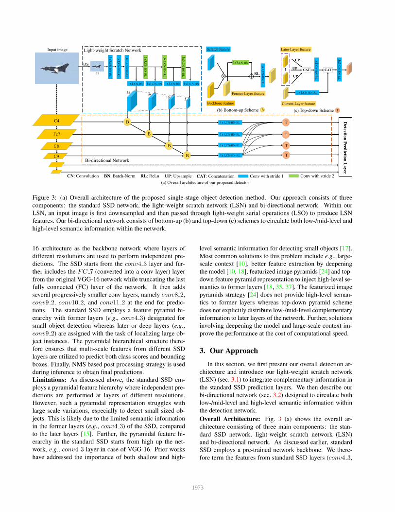
Figure 3: (a) Overall architecture of the proposed single-stage object detection method. Our approach consists of three

components: the standard SSD network, the light-weight scratch network (LSN) and bi-directional network. Within our

LSN, an input image is first downsampled and then passed through light-weight serial operations (LSO) to produce LSN

features. Our bi-directional network consists of bottom-up (b) and top-down (c) schemes to circulate both low-/mid-level and

high-level semantic information within the network.

16 architecture as the backbone network where layers of

different resolutions are used to perform independent pre-

dictions. The SSD starts from the conv4 3 layer and fur-

ther includes the FC 7 (converted into a conv layer) layer

from the original VGG-16 network while truncating the last

fully connected (FC) layer of the network. It then adds

several progressively smaller conv layers, namely conv8 2,

conv9 2, conv10 2, and conv11 2 at the end for predic-

tions. The standard SSD employs a feature pyramid hi-

erarchy with former layers (e.g., conv4 3) designated for

small object detection whereas later or deep layers (e.g.,

conv9 2) are assigned with the task of localizing large ob-

ject instances. The pyramidal hierarchical structure there-

fore ensures that multi-scale features from different SSD

layers are utilized to predict both class scores and bounding

boxes. Finally, NMS based post processing strategy is used

during inference to obtain final predictions.

Limitations: As discussed above, the standard SSD em-

ploys a pyramidal feature hierarchy where independent pre-

dictions are performed at layers of different resolutions.

However, such a pyramidal representation struggles with

large scale variations, especially to detect small sized ob-

jects. This is likely due to the limited semantic information

in the former layers (e.g., conv4 3) of the SSD, compared

to the later layers [15]. Further, the pyramidal feature hi-

erarchy in the standard SSD starts from high up the net-

work, e.g., conv4 3 layer in case of VGG-16. Prior works

have addressed the importance of both shallow and high-

level semantic information for detecting small objects [17].

Most common solutions to this problem include e.g., large-

scale context [10], better feature extraction by deepening

the model [10, 18], featurized image pyramids [24] and top-

down feature pyramid representation to inject high-level se-

mantics to former layers [18, 35, 37]. The featurized image

pyramids strategy [24] does not provide high-level seman-

tics to former layers whereas top-down pyramid scheme

does not explicitly distribute low-/mid-level complementary

information to later layers of the network. Further, solutions

involving deepening the model and large-scale context im-

prove the performance at the cost of computational speed.

3. Our Approach

In this section, we first present our overall detection ar-

chitecture and introduce our light-weight scratch network

(LSN) (sec. 3.1) to integrate complementary information in

the standard SSD prediction layers. We then describe our

bi-directional network (sec. 3.2) designed to circulate both

low-/mid-level and high-level semantic information within

the detection network.

Overall Architecture: Fig. 3 (a) shows the overall ar-

chitecture consisting of three main components: the stan-

dard SSD network, light-weight scratch network (LSN)

and bi-directional network. As discussed earlier, standard

SSD employs a pre-trained network backbone. We there-

fore term the features from standard SSD layers (conv4 3,

1973

FC 7, conv8 2, conv9 2, conv10 2, and conv11 2 ) as

backbone features since they originate from the pre-trained

network backbone. Similar to [21], we employ VGG-16

as the backbone network. The light-weight scratch net-

work (LSN) produces a low-/mid-level feature representa-

tion which is then injected into the backbone features of

subsequent standard prediction layers to improve their per-

formance. Afterwards, the resulting features from the cur-

rent and former layers are combined in the bottom-up fash-

ion inside our bi-directional network. The top-down scheme

in our bi-directional network contains independent parallel

connections to inject high-level semantic information from

later layers to former layers of the network.

Our bi-directional network has the following differences

compared to the feature pyramid network (FPN) [17] em-

ployed in several existing single-stage detectors [18, 36].

First, the bottom-up part of FPN follows the CNN’s pyra-

midal feature hierarchy which is also used in the standard

SSD framework. Both the bottom-up part of FPN and SSD

follow the feed-forward computation of backbone network

which builds a feature hierarchy. In addition to the bottom-

up part in FPN/standard SSD, the bottom-up scheme in our

bi-directional network propagates features from the former

to later layers in a cascaded fashion. Moreover, the top-

down pyramid in FPN performs a layer-by-layer fusion of

many CNN layers through cascaded operations. Instead

of cascaded/sequential layer-by-layer fusion, the prediction

layers are fused through independent parallel connections

in the top-down scheme of our bi-directional network.

3.1. Light­Weight Scratch Network

Our light-weight scratch network (LSN) is simple,

tightly linked to the standard SSD prediction layers and

is used to construct low-/mid-level feature representations,

termed as LSN features. We present the feature extraction

strategy used in our LSN followed by a description of the

LSN architecture.

LSN Feature Extraction: The feature extraction strategy

commonly employed in existing detection frameworks in-

volves extracting features from the network backbone, such

as VGG-16, in a repeated stack of multiple convolutional

blocks and max-pooling layers to produce semantically

strong features (see Fig. 4 (a)). Such a feature extraction

strategy is beneficial for the task of image classification that

prefers translation invariance. Different from image classi-

fication, object detection also requires accurate object delin-

eation for which local low-/mid-level feature (e.g., texture)

information is also crucial [38]. To compensate the loss of

information in the backbone features from the pre-trained

network, an alternative feature extraction scheme is utilized

in our LSN, as shown in Fig. 4 (b). First, an input image

is downsampled by a pooling operation to the target size

of first SSD prediction layer. The resulting downsampled

(b) LSN Feature ExtractionLSN Feature

LSO

Conv Block

LDS

Conv Block

(a) Backbone Feature ExtractionBackbone Feature

SDS SDS

SDS: Small Downsampling Stride LDS: Large Downsampling Stride

Figure 4: (a) Standard SSD feature extraction employs sev-

eral convolution blocks together with small downsampling

strides. (b) In our LSN, the input image is first downsam-

pled to the target size followed by light-weight serial oper-

ations (LSO) to produce LSN features.

image is then passed through light-weight serial operations

(LSO) including convolution, batch-norm and ReLU layers.

Note that our LSN is trained from scratch with random ini-

tialization. It follows a similar pyramidal feature hierarchy,

as in standard SSD, which is constructed as

Sp = {s1, s2, . . . , sn} (1)

where n is the number of feature pyramid levels selected

to match the size of standard SSD prediction layers. We

start by downsampling the input image I to the target size

of first SSD prediction layer (down-sampling rate is 8 in our

case). Then, we use the resulting downsampled image It to

generate the initial LSN feature sint(0):

sint(0) = ϕint(0)(It) (2)

where ϕint(0) denotes the serial operations, including

one 3×3 and one 1×1 conv. block. The initial feature

sint(0) is then used to generate an intermediate feature

set sint. The kth intermediate feature is obtained using

(k − 1)th intermediate feature:

sint(k) = ϕint(k)(sint(k−1)) (3)

where k = (1, . . . , n) and ϕint(k)(.) denotes one 3×3

conv. block. When k = 1, the (k−1)th intermediate feature

is equal to the initial LSN feature. Next, we apply a 1×1

conv. block to the kth level intermediate feature to generate

the kth level LSN feature of Sp,

sk = ϕtrans(k)(sint(k)) (4)

where ϕtrans(k)(.) denotes a 1×1 conv. block that trans-

forms the LSN feature channels to match the corresponding

standard SSD feature.

1974

3.2. Bi­directional Network

The bi-directional network circulates both low-/mid-

level and high-level semantic information within the de-

tection network and consists of bottom-up and top-down

schemes. The bottom-up scheme (see Fig. 3 (b)) combines

the backbone and LSN features and propagates the resulting

features of different levels in a feed-forward cascaded way

resulting in forward features. We refer this task as bottom-

up feature propagation (BFP). The kth level forward feature

is obtained by performing both tasks:

fk = φk((sk ⊗ ok)⊕ (wk−1fk−1))) (5)

where sk is the kth feature from LSN, ok represents the

kth original SSD prediction backbone feature, wk−1 de-

notes a 3 × 3 conv. block (without ReLU) with a stride of

2, fk−1 is the forward feature from the (k − 1)th level and

φk(.) denotes serial operations including ReLU and 3×3

conv. block. ⊗ and ⊕ denote element-wise multiplication

and addition, respectively. Note that BFP starts from the

second prediction layer. Therefore, the forward feature f1for the first prediction layer is in fact the fusion of the LSN

and backbone features, represented as:

f1 = φ1(s1 ⊗ o1) (6)

Finally, the forward features from all levels of the

bottom-up scheme are represented as a forward feature

pyramid:

Fp = {f1, f2, . . . , fn} (7)

As described above, the bottom-up scheme circulates the

low-/mid-level features in the forward direction. To further

inject the high-level semantic information from the later to

former layers, we introduce a top-down scheme (see Fig. 3

(c)). This scheme connects all the features from later lay-

ers to the current layer. It circulates high-level semantics

through independent parallel connections in the network.

The backward feature pyramid Bp is generated for pre-

diction as

Bp = {b1, b2, . . . , bn} (8)

We first employ several 1×1 conv. blocks to reduce the

feature channels of all the forward features in Fp. For kth

level, where k = (1, . . . , n − 1), the feature with reduced

channels is merged with all the higher level features to ob-

tain the backward feature bk for the final prediction,

bk = γk(∑

(Wkfk,Wmk(

n∑

k+1

µk(Wifi)))) (9)

where Wi, i = (k, . . . , n) is a 1×1 conv. block to reduce

the feature channels. Wmk is a 1×1 conv. block to merge

features from all the higher levels. µk is the upsampling

operation. γk(.) is a 3×3 conv. block to merge all the for-

ward features.∑

is a concatenation operation. Note that

the nth level forward feature is the highest level semantic

feature and does not require any semantic information from

former layers. This implies that the forward features of this

nth level are directly used as the prediction features.

4. Experiments

4.1. Datasets

MS COCO [19]: contains 80 object categories. It con-

sists of 160k images in total, with 80k training, 40k valida-

tion and 40k test-dev images. The training is performed on

120k images from the trainval set and evaluation is done on

the test-dev images. Here, the performance is evaluated by

following the standard MS COCO protocol where average

precision (AP) is measured by averaging over multiple IOU

thresholds, ranging from 0.5 to 0.95.

UAVDT dataset [9]: is a recently introduced large-scale

benchmark for object detection. The object of interest in

this benchmark is vehicle. The vehicle category consists

of car, truck and bus. The dataset contains 80k annotated

frames selected from 100 video sequences. The videos are

divided into training and testing sets with 30 and 70 se-

quences, respectively. We follow the same evaluation pro-

tocol provided by the respective authors [9].

4.2. Implementation Details

We employ VGG-16 [32], pre-trained on ImageNet [30]

as the backbone architecture in all baseline and UAVDT ex-

periments. In addition to VGG, we also report results with

ResNet-101 backbone on MS COCO dataset. Note that our

approach does not require any significant redesigning of the

underlying architecture, with change in backbone. When

going from VGG to ResNet backbone, only the number of

channels is changed. For both datasets, we adopt a warm-up

strategy for the first six epochs. The initial learning rate is

set to 2 × 10−3 and gradually decreased to 2 × 10−4 and

2 × 10−5 at 90 and 120 epochs, respectively. We employ

the default settings as in the standard SSD method [21] for

loss function, scales and aspect ratios of the defaults boxes

and data augmentation. In our experiments, the weight de-

cay is set to 0.0005 and the momentum to 0.9. For both

datasets, the batch-size is 32. A total number of 160 epochs

are performed for both two datasets.

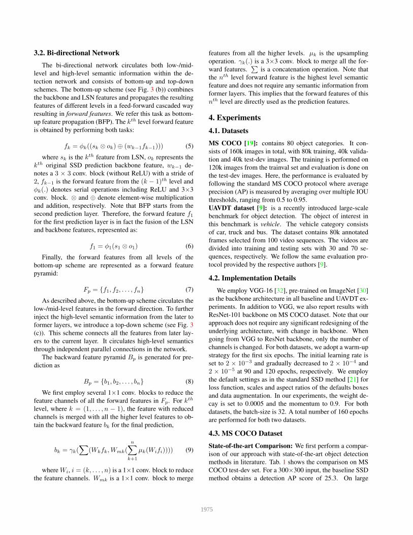
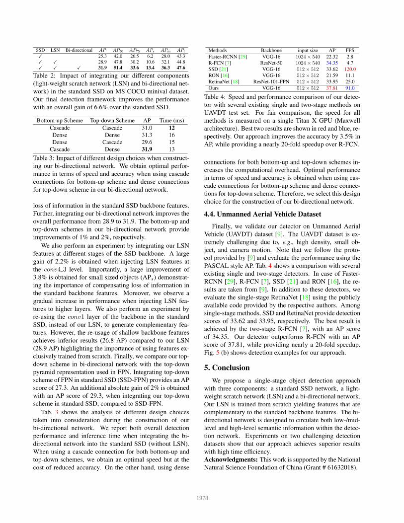
4.3. MS COCO Dataset

State-of-the-art Comparison: We first perform a compar-

ison of our approach with state-of-the-art object detection

methods in literature. Tab. 1 shows the comparison on MS

COCO test-dev set. For a 300×300 input, the baseline SSD

method obtains a detection AP score of 25.3. On large

1975

Methods Backbone Input size Time(ms) AP AP50 AP75 APs APm APl

Two-Stage Detector:

Faster-RCNN [29] VGG-16 ∼ 1000× 600 147 24.2 45.3 23.5 7.7 26.4 37.1

Faster-FPN [17] ResNet-101-FPN ∼ 1000× 600 240 36.2 59.1 39.0 18.2 39.0 48.2

R-FCN [7] ResNet-101 ∼ 1000× 600 110 29.9 51.9 - 10.8 32.8 45.0

Deformable R-FCN [8] ResNet-101 ∼ 1000× 600 125 34.5 55.0 - 14.0 37.7 50.3

Mask-RCNN [13] ResNeXt-101-FPN ∼ 1280× 800 210 39.8 62.3 43.4 22.1 43.2 51.2

Cascade R-CNN [2] ResNet-101-FPN ∼ 1280× 800 141 42.8 62.1 46.3 23.7 45.5 55.2

SNIP [33] DPN-98 - - 45.7 67.3 51.1 29.3 48.8 57.1

Single-Stage Detector:

SSD [21] VGG-16 300× 300 12 25.3 42.0 26.5 6.2 28.0 43.3

SSD [10] ResNet-101 321× 321 20 28.0 45.4 29.3 6.2 28.3 49.3

DSSD [10] ResNet-101 321× 321 - 28.0 46.1 29.2 7.4 28.1 47.6

RefineDet [36] VGG-16 320× 320 26 29.4 49.2 31.3 10.0 32.0 44.4

RefineDet [36] ResNet-101 320× 320 - 32.0 51.4 34.2 10.5 34.7 50.4

RFBNet [20] VGG-16 300× 300 15 30.3 49.3 31.8 11.8 31.9 45.9

EFIP [24] VGG-16 300× 300 14 30.0 48.8 31.7 10.9 32.8 46.3

Ours VGG-16 300× 300 13 32.0 51.5 33.8 12.6 34.9 47.0

Ours ResNet-101 300× 300 19 34.3 54.1 36.6 13.2 38.2 50.7

YOLOv2 [27] Darknet 544× 544 25 21.6 44.0 19.2 5.0 22.4 35.5

YOLOv3 [28] DarkNet-53 608× 608 51 33.0 57.9 34.4 18.3 35.4 41.9

SSD [21] VGG-16 512× 512 28 28.8 48.5 30.3 10.9 31.8 43.5

SSD [10] ResNet-101 513× 513 32 31.2 50.4 33.3 10.2 34.5 49.8

DSSD [10] ResNet-101 513× 513 156 33.2 53.3 35.2 13.0 35.4 51.1

RefineDet [36] VGG-16 512× 512 45 33.0 54.5 35.5 16.3 36.3 44.3

RefineDet [36] ResNet-101 512× 512 - 36.4 57.5 39.5 16.6 39.9 51.4

Rev-Dense [35] VGG-16 512× 512 - 31.2 52.9 32.4 15.5 32.9 43.9

RFBNet [20] VGG-16 512× 512 30 33.8 54.2 35.9 16.2 37.1 47.4

RFBNet-E [20] VGG-16 512× 512 33 34.4 55.7 36.4 17.6 37.0 47.6

RetinaNet [18] ResNet-101-FPN ∼ 832× 500 90 34.4 55.7 36.8 14.7 37.1 47.4

EFIP [24] VGG-16 512× 512 29 34.6 55.8 36.8 18.3 38.2 47.1

RetinaNet+AP-Loss [5] ResNet-101-FPN ∼ 832× 500 91 37.4 58.6 40.5 17.3 40.8 51.9

Ours VGG-16 512× 512 26 36.2 56.6 38.7 19.0 39.9 48.8

Ours ResNet-101 512× 512 32 37.3 58.5 39.7 19.7 42.8 50.1

Table 1: Comparison (in terms of AP) of our detector with state-of-the-art methods on MS COCO test-dev set. Our approach

achieves impressive performance for both 300× 300 and 512× 512 inputs. When using a 300× 300 input, our detector with

ResNet-101 backbone surpasses existing single-stage methods in terms of overall accuracy while operating at an inference

time of 19 milliseconds (ms). Our detector also outperforms existing single-stage methods on both small and medium objects.

objects (APl), the baseline SSD provides a decent perfor-

mance of 43.3 AP. However, its performance significantly

deteriorates to 6.2 AP on small objects (APs). Our ap-

proach, using the same VGG backbone, provides a signif-

icant overall gain of 6.7% in detection AP over the base-

line SSD. Importantly, our detector achieves more than dou-

ble the detection performance on small objects, compared

to the SSD framework. Similarly, a large improvement in

detection performance is also obtained on medium objects

(APm). Among existing methods, RefineDet [36] and RFB-

Net [20] with VGG backbone achieve AP scores of 29.4 and

30.3, respectively. Our detector with the same backbone

achieves superior results compared to both these methods.

For a 512×512 input, the baseline SSD achieves a detec-

tion AP score of 28.8. Our detector with same VGG back-

bone provides a significant overall gain of 7.4% in AP, over

the baseline SSD. Among existing methods, RetinaNet [18]

and RetinaNet+AP-Loss [5] provide detection AP scores of

34.4 and 37.4, respectively. However, both approaches are

slower with inference times of ∼ 90ms. Our approach with

the same ResNet-101 backbone (without FPN) achieves

comparable performance with a detection AP score of 37.3,

while operating at significantly faster inference time of 32

millisecond (ms) on a single Titan X GPU.

Although two-stage methods achieve superior accuracy,

they are computationally expensive, often require a large in-

put resolution and mostly take more than 100ms to process

an image. For instance, Cascade R-CNN [2] achieves 42.8

AP but requires 141ms to process an image. Our detector

provides promising accuracy with high time efficiency.

1976

a: COCO detection results b: UAVDT detection resultsFigure 5: Qualitative detection results of our approach on (a) COCO test-dev (corresponding to 36.2 AP) and (b) UAVDT test

set (corresponding to 37.8 AP). Most of examples depict the performance on small objects. The black regions are ignored in

UAVDT dataset images [9]. Our detector is able to accurately localize small objects in these challenging scenes.

Figure 6: Error analysis comparison between the baseline

SSD (top row) and our detector (bottom row). The compar-

ison is shown for both overall and small sized objects. Each

sub-image contains plots that describe a series of precision

recall curves computed using different evaluation settings

[19]. Further, the area under each curve is presented (brack-

ets) in the legend. Our approach significantly improves the

detection performance over the baseline SSD framework.

Qualitative Analysis: A large number of small sized ob-

jects (41% of all objects) in the MS COCO dataset makes it

especially suitable to evaluate the performance for small ob-

ject detection. An object instance is considered small here

if the area is < 322. We perform a further analysis of our

detector by employing the error analysis protocol provided

by [19]. The error analysis plots of the baseline SSD (top

row) and our approach (bottom) with VGG backbone for

both overall and small objects are shown in Fig. 6. As de-

fined by [19], the plots in each sub-image depict a series

of precision recall curves employing different settings. The

area under each curve is shown (brackets) in the legends.

In case of the baseline SSD (top row), the overall AP at

IoU=0.50 is 0.482 and removing the background false pos-

itives will result in improving the performance to 0.789 AP.

For our approach (bottom row), the overall AP at IoU=0.50is 0.560 and removing the background false positives will

increase the performance to 0.847 AP. In case of small sized

objects, our approach provides more notable improvements

in performance, compared to SSD. For instance, the results

are significantly improved from 0.231 obtained by SSD to

0.357 at IoU=0.50 for our method. Further, Fig. 5 (a) shows

detection examples with our approach.

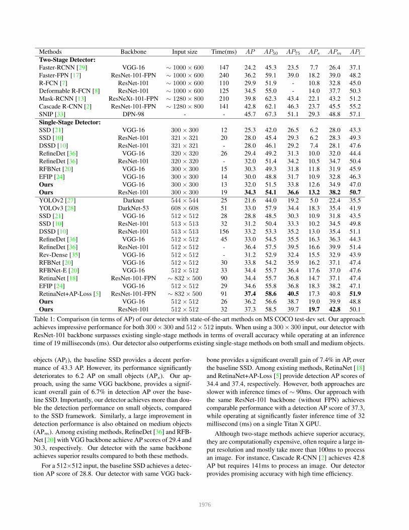
Ablation Study: We perform an ablation study on the MS

COCO-minival and report results using a 300×300 input

with VGG backbone. We first validate the impact of our

proposed components: light-weight scratch network (LSN)

(sec. 3.1) and bi-directional network (sec. 3.2). Note that

our bi-directional network consists of bottom-up and top-

down schemes to circulate both low-/mid-level and high-

levelsemantic information within the detection network.

Tab. 2 shows the impact of our LSN and bi-directional net-

work. The standard SSD provides a detection AP score of

25.3. Integrating our LSN significantly improves the detec-

tion performance with AP score of 28.9. Notably, a sig-

nificant gain of 4.4% is obtained compared to the baseline

SSD for small sized objects (APs). The large gain in perfor-

mance especially for small (APs) and medium (APm) ob-

jects shows the impact of our LSN on compensating for the

1977

SSD LSN Bi-directional AP AP50 AP75 APs APm APl

X 25.3 42.0 26.5 6.2 28.0 43.3

X X 28.9 47.8 30.2 10.6 32.1 44.8

X X X 31.9 51.4 33.6 13.4 36.3 47.6

Table 2: Impact of integrating our different components

(light-weight scratch network (LSN) and bi-directional net-

work) in the standard SSD on MS COCO minival dataset.

Our final detection framework improves the performance

with an overall gain of 6.6% over the standard SSD.

Bottom-up Scheme Top-down Scheme AP Time (ms)

Cascade Cascade 31.0 12

Dense Dense 31.3 16

Dense Cascade 29.6 15

Cascade Dense 31.9 13

Table 3: Impact of different design choices when construct-

ing our bi-directional network. We obtain optimal perfor-

mance in terms of speed and accuracy when using cascade

connections for bottom-up scheme and dense connections

for top-down scheme in our bi-directional network.

loss of information in the standard SSD backbone features.

Further, integrating our bi-directional network improves the

overall performance from 28.9 to 31.9. The bottom-up and

top-down schemes in our bi-directional network provide

improvements of 1% and 2%, respectively.

We also perform an experiment by integrating our LSN

features at different stages of the SSD backbone. A large

gain of 2.2% is obtained when injecting LSN features at

the conv4 3 level. Importantly, a large improvement of

3.8% is obtained for small sized objects (APs) demonstrat-

ing the importance of compensating loss of information in

the standard backbone features. Moreover, we observe a

gradual increase in performance when injecting LSN fea-

tures to higher layers. We also perform an experiment by

re-using the conv1 layer of the backbone in the standard

SSD, instead of our LSN, to generate complementary fea-

tures. However, the re-usage of shallow backbone features

achieves inferior results (26.8 AP) compared to our LSN

(28.9 AP) highlighting the importance of using features ex-

clusively trained from scratch. Finally, we compare our top-

down scheme in bi-direcional network with the top-down

pyramid representation used in FPN. Integrating top-down

scheme of FPN in standard SSD (SSD-FPN) provides an AP

score of 27.3. An additional absolute gain of 2% is obtained

with an AP score of 29.3, when integrating our top-down

scheme in standard SSD, compared to SSD-FPN.

Tab. 3 shows the analysis of different design choices

taken into consideration during the construction of our

bi-directional network. We report both overall detection

performance and inference time when integrating the bi-

directional network into the standard SSD (without LSN).

When using a cascade connection for both bottom-up and

top-down schemes, we obtain an optimal speed but at the

cost of reduced accuracy. On the other hand, using dense

Methods Backbone input size AP FPS

Faster-RCNN [29] VGG-16 1024× 540 22.32 2.8

R-FCN [7] ResNet-50 1024× 540 34.35 4.7

SSD [21] VGG-16 512× 512 33.62 120.0

RON [16] VGG-16 512× 512 21.59 11.1

RetinaNet [18] ResNet-101-FPN 512× 512 33.95 25.0

Ours VGG-16 512× 512 37.81 91.0

Table 4: Speed and performance comparison of our detec-

tor with several existing single and two-stage methods on

UAVDT test set. For fair comparison, the speed for all

methods is measured on a single Titan X GPU (Maxwell

architecture). Best two results are shown in red and blue, re-

spectively. Our approach improves the accuracy by 3.5% in

AP, while providing a nearly 20-fold speedup over R-FCN.

connections for both bottom-up and top-down schemes in-

creases the computational overhead. Optimal performance

in terms of speed and accuracy is obtained when using cas-

cade connections for bottom-up scheme and dense connec-

tions for top-down scheme. Therefore, we select this design

choice for the construction of our bi-directional network.

4.4. Unmanned Aerial Vehicle Dataset

Finally, we validate our detector on Unmanned Aerial

Vehicle (UAVDT) dataset [9]. The UAVDT dataset is ex-

tremely challenging due to, e.g., high density, small ob-

ject, and camera motion. Note that we follow the proto-

col provided by [9] and evaluate the performance using the

PASCAL style AP. Tab. 4 shows a comparison with several

existing single and two-stage detectors. In case of Faster-

RCNN [29], R-FCN [7], SSD [21] and RON [16], the re-

sults are taken from [9]. In addition to these detectors, we

evaluate the single-stage RetinaNet [18] using the publicly

available code provided by the respective authors. Among

single-stage methods, SSD and RetinaNet provide detection

scores of 33.62 and 33.95, respectively. The best result is

achieved by the two-stage R-FCN [7], with an AP score

of 34.35. Our detector outperforms R-FCN with an AP

score of 37.81, while providing nearly a 20-fold speedup.

Fig. 5 (b) shows detection examples for our approach.

5. Conclusion

We propose a single-stage object detection approach

with three components: a standard SSD network, a light-

weight scratch network (LSN) and a bi-directional network.

Our LSN is trained from scratch yielding features that are

complementary to the standard backbone features. The bi-

directional network is designed to circulate both low-/mid-

level and high-level semantic information within the detec-

tion network. Experiments on two challenging detection

datasets show that our approach achieves superior results

with high time efficiency.

Acknowledgments: This work is supported by the National

Natural Science Foundation of China (Grant # 61632018).

1978

References

[1] Yancheng Bai, Yongqiang Zhang, Mingli Ding, and Bernard

Ghanem. Sod-mtgan: Small object detection via multi-task

generative adversarial network. In ECCV, 2018. 2

[2] Zhaowei Cai and Nuno Vasconcelos. Cascade r-cnn: Delving

into high quality object detection. In CVPR, 2018. 6

[3] Jiale Cao, Yanwei Pang, Jungong Han, and Xuelong Li. Hi-

erarchical shot detector. In ICCV, 2019. 1

[4] Jiale Cao, Yanwei Pang, and Xuelong Li. Triply supervised

decoder networks for joint detection and segmentation. In

CVPR, 2019. 1, 2

[5] Kean Chen, Jianguo Li, Weiyao Lin, John See, Ji Wang,

Lingyu Duan, Zhibo Chen, Changwei He, and Junni Zou.

Towards accurate one-stage object detection with ap-loss. In

CVPR, 2019. 6

[6] Hisham Cholakkal, Guolei Sun, Fahad Shahbaz Khan, and

Ling Shao. Object counting and instance segmentation with

image-level supervision. In CVPR, 2019. 1

[7] Jifeng Dai, Yi Li, Kaiming He, and Jian Sun. R-FCN: Object

detection via region-based fully convolutional networks. In

NIPS, 2016. 6, 8

[8] Jifeng Dai, Haozhi Qi, Yuwen Xiong, Yi Li, Guodong

Zhang, Han Hu, and Yichen Wei. Deformable convolutional

networks. In ICCV, 2017. 6

[9] Dawei Du, Yuankai Qi, Hongyang Yu, Yifan Yang, Kaiwen

Duan, Guorong Li, Weigang Zhang, Qingming Huang, and

Qi Tian. The unmanned aerial vehicle benchmark: Object

detection and tracking. In ECCV, 2018. 1, 5, 7, 8

[10] Cheng-Yang Fu, Wei Liu, Ananth Ranga, Ambrish Tyagi,

Alexander, and C. Berg. Dssd : Deconvolutional single shot

detector. arXiv preprint arXiv:1701.06659, 2017. 2, 3, 6

[11] Ross Girshick. Fast r-cnn. In ICCV, 2015. 2

[12] Kaiming He, Ross Girshick, and Piotr Dollar. Rethinking im-

agenet pre-training. arXiv preprint arXiv:1811.08883, 2018.

2

[13] Kaiming He, Georgia Gkioxari, Piotr Dollar, and Ross Gir-

shick. Mask R-CNN. In ICCV, 2017. 6

[14] Kaiming He, Xiangyu Zhang, Shaoqing Ren, and Jian Sun.

Spatial pyramid pooling in deep convolutional networks for

visual recognition. In ECCV, 2014. 2

[15] Jonathan Huang, Vivek Rathod, Chen Sun, Menglong Zhu,

Anoop Korattikara, Alireza Fathi, Ian Fischer, Zbigniew Wo-

jna, Yang Song, Sergio Guadarrama, and Kevin Murphy.

Speed/accuracy trade-offs for modern convolutional object

detectors. In CVPR, 2017. 2, 3

[16] Tao Kong, Fuchun Sun, Anbang Yao, Huaping Liu, Ming Lu,

and Yurong Chen. Ron: Reverse connection with objectness

prior networks for object detection. In CVPR, 2017. 8

[17] Tsung-Yi Lin, Piotr Dollar, Ross Girshick, Kaiming He,

Bharath Hariharan, and Serge Belongie. Feature pyramid

networks for object detection. In CVPR, 2017. 2, 3, 4, 6

[18] Tsung-Yi Lin, Priya Goyal, Ross Girshick, Kaiming He, and

Piotr Dollr. Focal loss for dense object detection. In ICCV,

2017. 1, 2, 3, 4, 6, 8

[19] Tsung-Yi Lin, Michael Maire, Serge Belongie, James Hays,

Pietro Perona, Deva Ramanan, Piotr Dollr, and C. Lawrence

Zitnick. Microsoft coco: Common objects in context. In

ECCV, 2014. 1, 2, 5, 7

[20] Songtao Liu, Di Huang, and Yunhong Wang. Receptive field

block net for accurate and fast object detection. In ECCV,

2018. 2, 6

[21] Wei Liu, Dragomir Anguelov, Dumitru Erhan, Christian

Szegedy, Scott Reed, Cheng-Yang Fu, and Alexander C.

Berg. SSD: Single shot multibox detector. In ECCV, 2016.

1, 2, 4, 5, 6, 8

[22] Yanwei Pang, Jiale Cao, and Xuelong Li. Cascade learning

by optimally partitioning. IEEE Transactions on Cybernet-

ics, 47(12):4148–4161, 2017. 1

[23] Yanwei Pang, Manli Sun, Xiaoheng Jiang, and Xuelong

Li. Convolution in convolution for network in network.

IEEE Transactions on Neural Networks and Learning Sys-

tem, 29(5):1587–1597, 2018. 1

[24] Yanwei Pang, Tiancai Wang, Rao Muhammad Anwer, Fa-

had Shahbaz Khan, and Ling Shao. Efficient featurized im-

age pyramid network for single shot detector. In CVPR,

2019. 2, 3, 6

[25] Yanwei Pang, Jin Xie, and Xuelong Li. Visual haze removal

by a unified generative adversarial network. IEEE Transac-

tions on Circuits and Systems for Video Technology, 2018.

1

[26] Joseph Redmon, Santosh Divvala, Ross Girshick, and Ali

Farhadi. You only look once: Unified, real-time object de-

tection. In CVPR, 2016. 1

[27] Joseph Redmon and Ali Farhadi. Yolo9000:better, faster,

stronger. In CVPR, 2017. 1, 6

[28] Joseph Redmon and Ali Farhadi. Yolov3: An incremental

improvement. arXiv preprint arXiv:1804.02767, 2018. 1, 2,

6

[29] Shaoqing Ren, Kaiming He, Ross Girshick, and Jian Sun.

Faster R-CNN: towards real-time object detection with re-

gion proposal networks. In NIPS, 2015. 2, 6, 8

[30] Olga Russakovsky, Jia Deng, Hao Su, Jonathan Krause, San-

jeev Satheesh, Sean Ma, Zhiheng Huang, Andrej Karpathy,

Aditya Khosla, Michael Bernstein, Alexander C. Berg, and

Li Fei-Fei. Imagenet large scale visual recognition challenge.

In IJCV, 2015. 2, 5

[31] Fahad Shahbaz Khan, Xu Jiaolong, Joost van de Wei-

jer, Andrew Bagdanov, and Antonio Anwer, Rao Muham-

mad Lopez. Recognizing actions through action-specific

person detection. IEEE Transactions on Image Processing,

24(11):4422–4432, 2015. 2

[32] Karen Simonyan and Andrew Zisserman. Very deep convo-

lutional networks for large-scale image recognition. In NIPS,

2014. 5

[33] Bharat Singh and Larry Davis. An analysis of scale invari-

ance in object detection - snip. In CVPR, 2018. 6

[34] Hanqing Sun and Yanwei Pang. Glancenets-efficient convo-

lutional neural networks with adaptive hard example mining.

SCIENCE CHINA Information Sciences, 61(10), 2018. 1

[35] Yongjian Xin, Shuhui Wang, Liang Li, Weigang Zhangg, and

Qingming Huang. Reverse densely connected feature pyra-

mid network for object detection. In ACCV, 2018. 3, 6

1979

[36] Shifeng Zhang, Longyin Wen, Xiao Bian, Zhen Lei, and

Stan Z. Li. Single-shot refinement neural network for object

detection. In CVPR, 2018. 2, 4, 6

[37] Zhishuai Zhang, Siyuan Qiao, Cihang Xie, Wei Shen, Bo

Wang, and Alan Yuille. Single-shot object detection with

enriched semantics. In CVPR, 2018. 3

[38] Rui Zhu, Shifeng Zhang, Xiaobo Wang, Longyin Wen,

Hailin Shi, Liefeng Bo, and Tao Mei. Scratchdet: Training

single-shot object detectors from scratch. In CVPR, 2019. 2,

4

1980