lecture 1: the greedy method
DESCRIPTION
Lecture 1: The Greedy Method. 主講人 : 虞台文. Content. What is it? Activity Selection Problem Fractional Knapsack Problem Minimum Spanning Tree Kruskal’s Algorithm Prim’s Algorithm Shortest Path Problem Dijkstra’s Algorithm Huffman Codes. Lecture 1: The Greedy Method. What is it?. - PowerPoint PPT PresentationTRANSCRIPT
Lecture 1: The Greedy Method
主講人 :虞台文
Content
What is it? Activity Selection Problem Fractional Knapsack Problem Minimum Spanning Tree
– Kruskal’s Algorithm– Prim’s Algorithm
Shortest Path Problem– Dijkstra’s Algorithm
Huffman Codes
Lecture 1: The Greedy Method
What is it?
The Greedy Method
A greedy algorithm always makes the choice that looks best at the moment
For some problems, it always give a globally optimal solution.
For others, it may only give a locally optimal one.

Main Components
Configurations– different choices, collections, or values to find
Objective function– a score assigned to configurations, which we w
ant to either maximize or minimize

Example: Making Change
Problem– A dollar amount to reach and a collection of coin
amounts to use to get there. Configuration
– A dollar amount yet to return to a customer plus the coins already returned
Objective function– Minimize number of coins returned.
Greedy solution– Always return the largest coin you can
Is the solution always optimal?
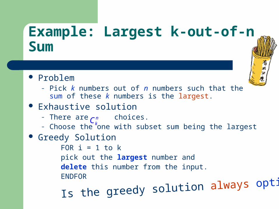
Example: Largest k-out-of-n Sum
Problem– Pick k numbers out of n numbers such that the sum of
these k numbers is the largest. Exhaustive solution
– There are choices.– Choose the one with subset sum being the largest
Greedy SolutionFOR i = 1 to k
pick out the largest number and delete this number from the
input.ENDFORIs the greedy solution always optimal?
nkC
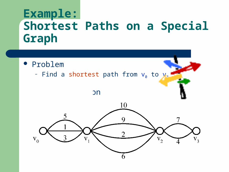
Example:Shortest Paths on a Special Graph
Problem– Find a shortest path from v0 to v3
Greedy Solution
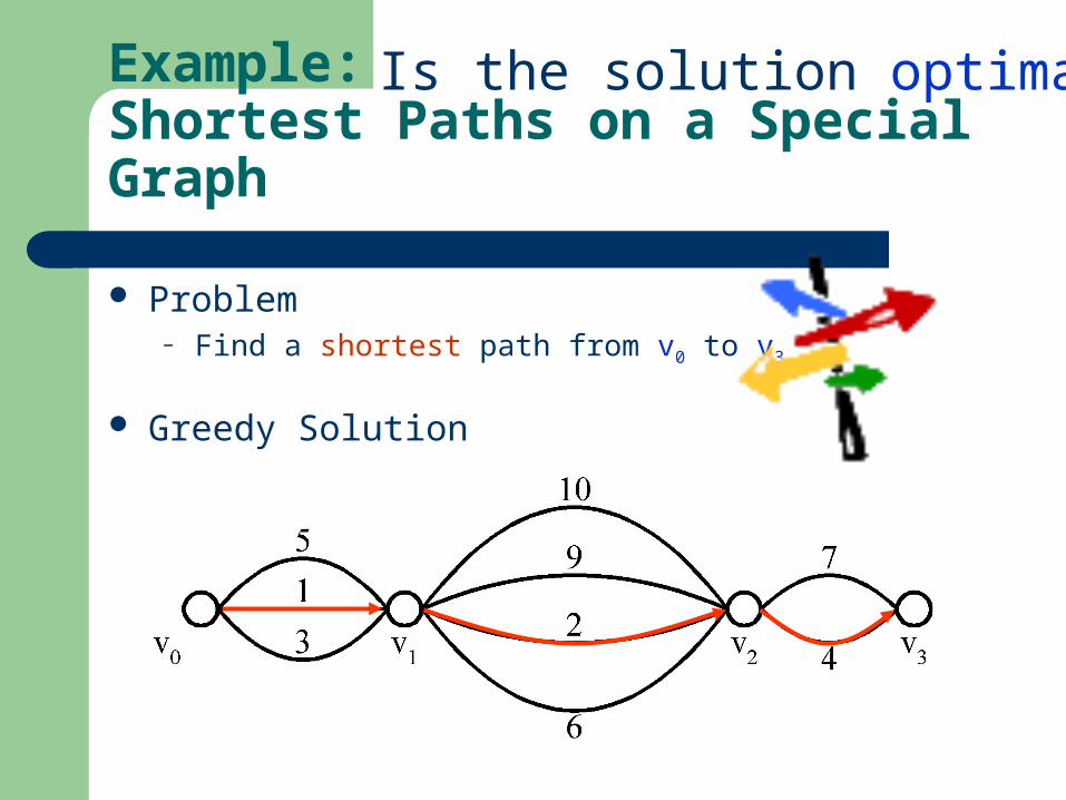
Example:Shortest Paths on a Special Graph
Problem– Find a shortest path from v0 to v3
Greedy Solution
Is the solution optimal?
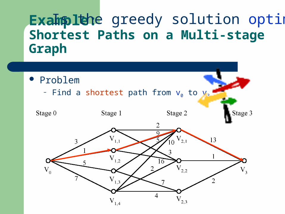
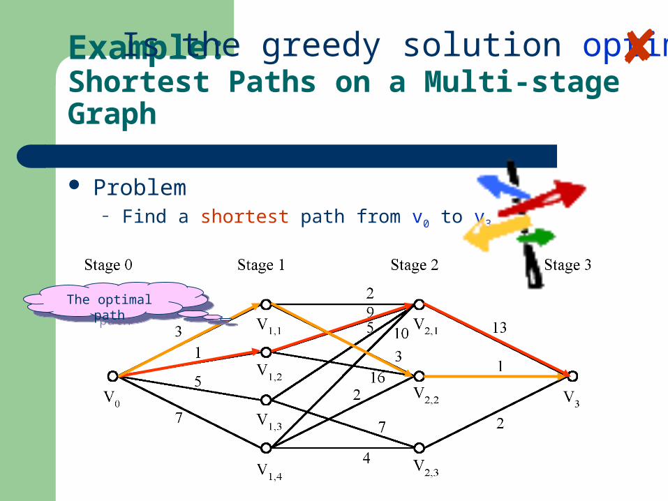
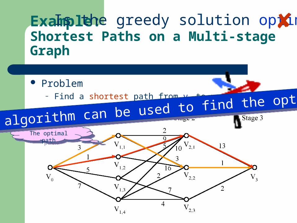
Example:Shortest Paths on a Multi-stage Graph
Problem– Find a shortest path from v0 to v3
Is the greedy solution optimal?
Example:Shortest Paths on a Multi-stage Graph
Problem– Find a shortest path from v0 to v3
Is the greedy solution optimal?
The optimal path
The optimal path
Example:Shortest Paths on a Multi-stage Graph
Problem– Find a shortest path from v0 to v3
Is the greedy solution optimal?
The optimal path
The optimal path
What algorithm can be used to find the optimum?
What algorithm can be used to find the optimum?
Advantage and Disadvantageof the Greedy Method
Advantage– Simple– Work fast when they work
Disadvantage– Not always work Short term solutions can
be disastrous in the long term– Hard to prove correct
Lecture 1: The Greedy Method
Activity Selection Problem
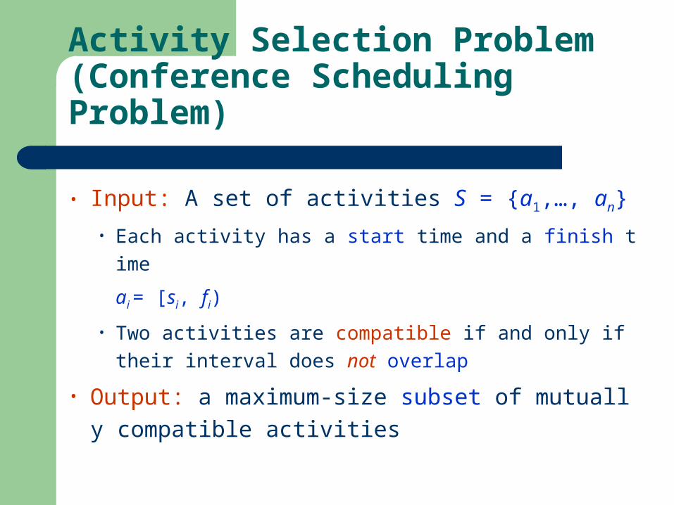
Activity Selection Problem(Conference Scheduling Problem)
• Input: A set of activities S = {a1,…, an}
• Each activity has a start time and a finish timeai = [si, fi)
• Two activities are compatible if and only if their interval does not overlap
• Output: a maximum-size subset of mutually compatible activities
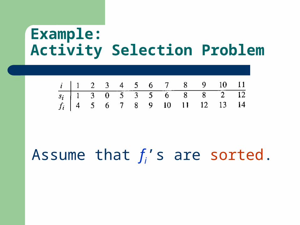
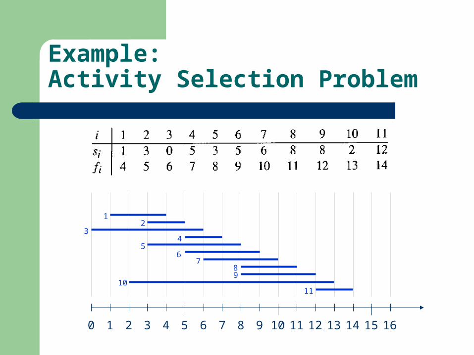
Example:Activity Selection Problem
Assume that fi’s are sorted.
Example:Activity Selection Problem
0 1 2 3 4 5 6 7 8 9 10 11 12 13 14 15 16
12
34
56
789
1011

Example:Activity Selection Problem
0 1 2 3 4 5 6 7 8 9 10 11 12 13 14 15 16
12
34
56
789
1011
Is the solution optimal?
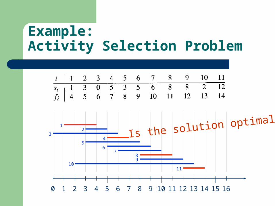
Example:Activity Selection Problem
0 1 2 3 4 5 6 7 8 9 10 11 12 13 14 15 16
12
34
56
789
1011
Is the solution optimal?
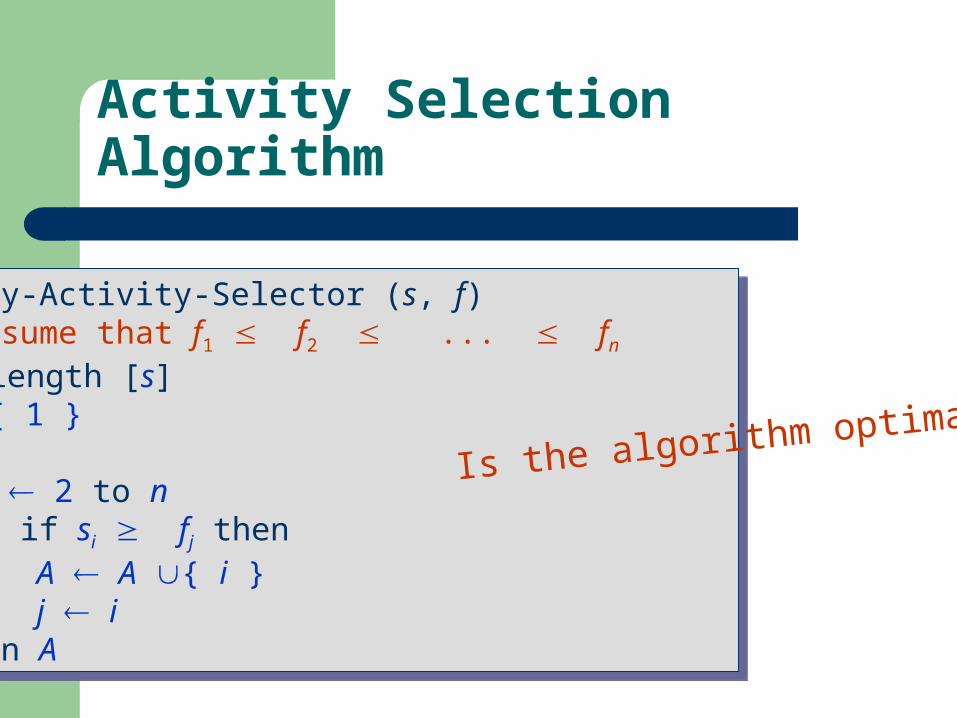
Activity Selection Algorithm
Greedy-Activity-Selector (s, f) // Assume that f1 f2 ... fn n length [s] A { 1 } j 1 for i 2 to n if si fj then
A A { i } j i
return A
Greedy-Activity-Selector (s, f) // Assume that f1 f2 ... fn n length [s] A { 1 } j 1 for i 2 to n if si fj then
A A { i } j i
return A
Is the algorithm optimal?
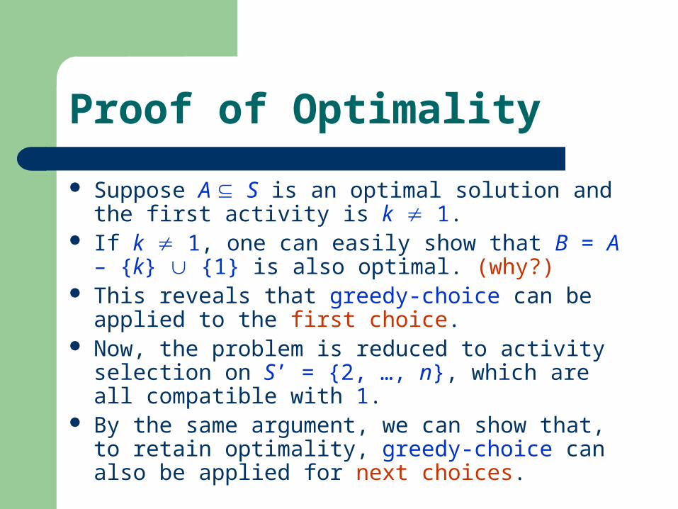
Proof of Optimality
Suppose A S is an optimal solution and the first activity is k 1.
If k 1, one can easily show that B = A – {k} {1} is also optimal. (why?)
This reveals that greedy-choice can be applied to the first choice.
Now, the problem is reduced to activity selection on S’ = {2, …, n}, which are all compatible with 1.
By the same argument, we can show that, to retain optimality, greedy-choice can also be applied for next choices.
Lecture 1: The Greedy Method
Fractional Knapsack Problem
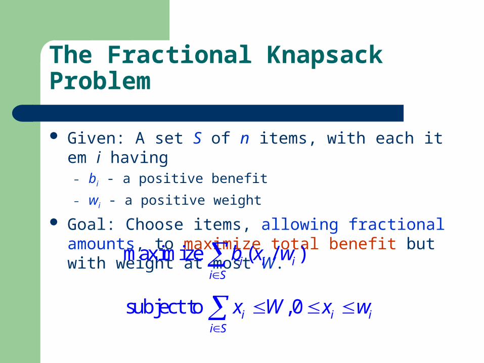
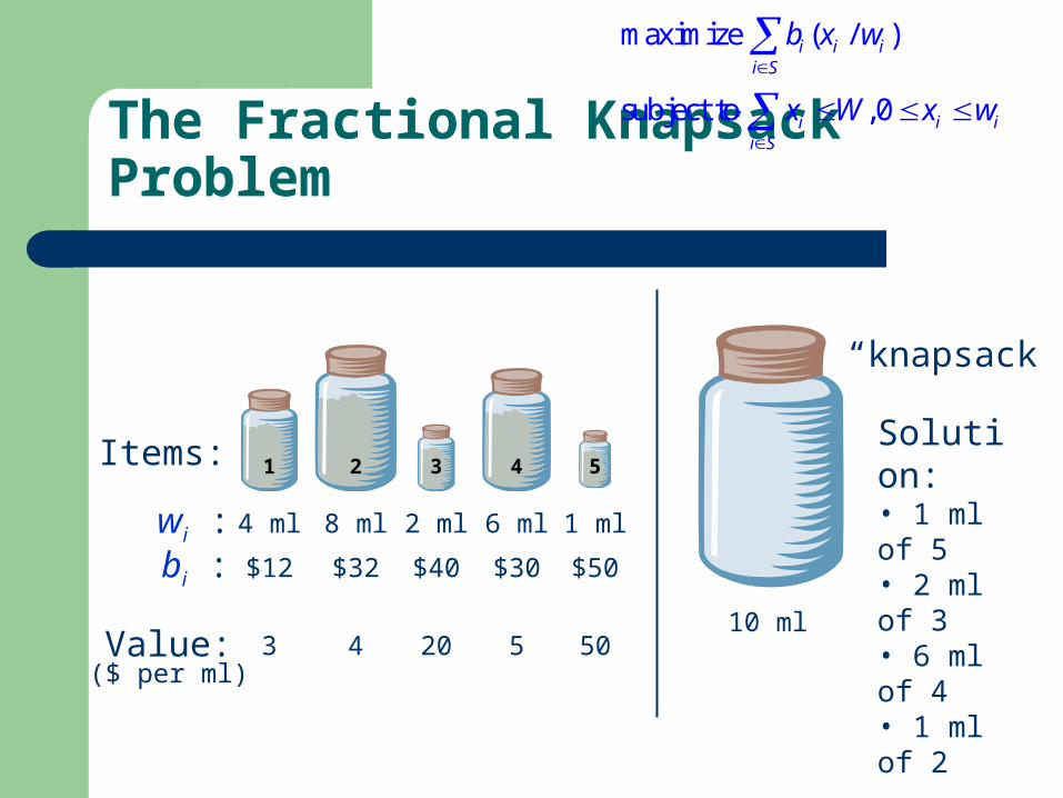
The Fractional Knapsack Problem
Given: A set S of n items, with each item i having– bi - a positive benefit– wi - a positive weight
Goal: Choose items, allowing fractional amounts, to maximize total benefit but with weight at most W. maximize ( / )i i i
i S
b x w
subject to ,0i i ii S
x W x w
The Fractional Knapsack Problem
maximize ( / )i i ii S
b x w
subject to ,0i i ii S
x W x w
wi :bi :
1 2 3 4 5
4 ml 8 ml 2 ml 6 ml 1 ml
$12 $32 $40 $30 $50
Items:
3Value:($ per ml)
4 20 5 5010 ml
Solution:• 1 ml of 5• 2 ml of 3• 6 ml of 4• 1 ml of 2
“knapsack”
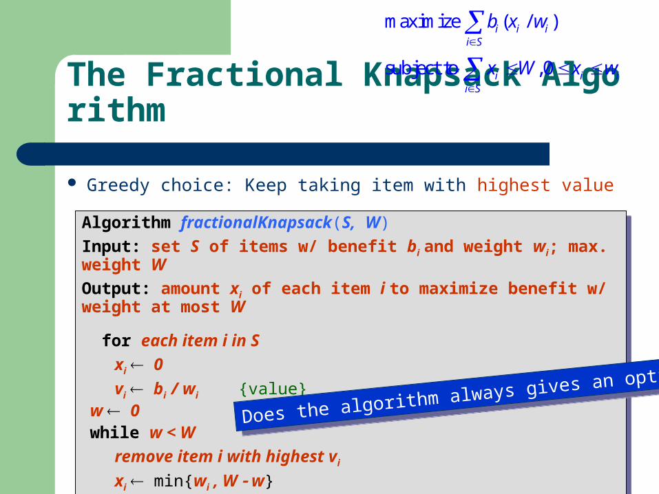
The Fractional Knapsack Algorithm
maximize ( / )i i ii S
b x w
subject to ,0i i ii S
x W x w
Greedy choice: Keep taking item with highest value
Algorithm fractionalKnapsack(S, W)
Input: set S of items w/ benefit bi and weight wi; max. weight W
Output: amount xi of each item i to maximize benefit w/ weight at most W
for each item i in S
xi 0
vi bi / wi {value}w 0 {total weight}
while w < W
remove item i with highest vi
xi min{wi , W w}
w w + min{wi , W w}
Does the algorithm always gives an optimum?
Does the algorithm always gives an optimum?
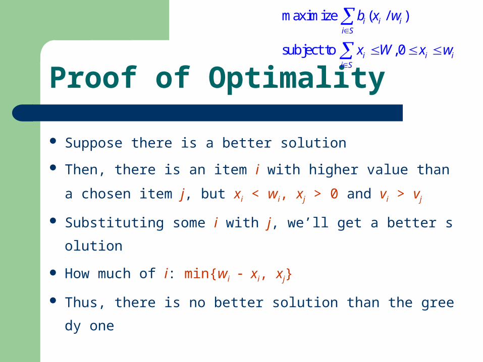
Proof of Optimality
maximize ( / )i i ii S
b x w
subject to ,0i i ii S
x W x w
Suppose there is a better solution Then, there is an item i with higher value than a chos
en item j, but xi < wi, xj > 0 and vi > vj
Substituting some i with j, we’ll get a better solution
How much of i: min{wi xi, xj}
Thus, there is no better solution than the greedy one
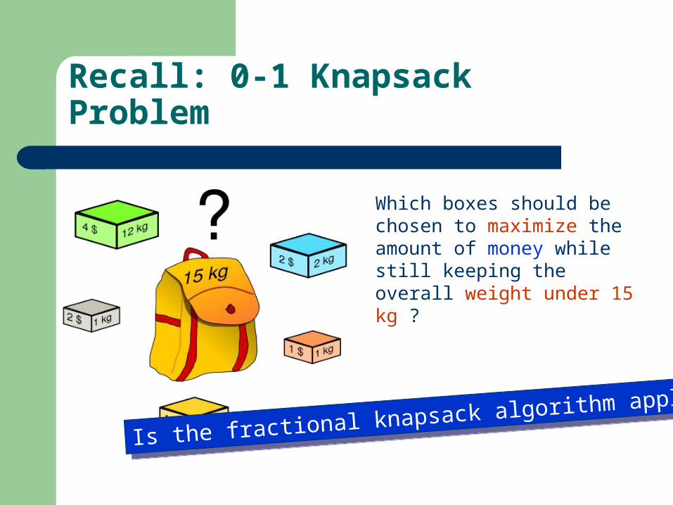
Recall: 0-1 Knapsack Problem
Which boxes should be chosen to maximize the amount of money while still keeping the overall weight under 15 kg ?
Is the fractional knapsack algorithm applicable?
Is the fractional knapsack algorithm applicable?
Exercise
1. Construct an example show that the fractional knapsack algorithm doesn’t give the optimal solution when applying it to the 0-1 knapsack problem.

Lecture 1: The Greedy Method
MinimumSpanning Tree
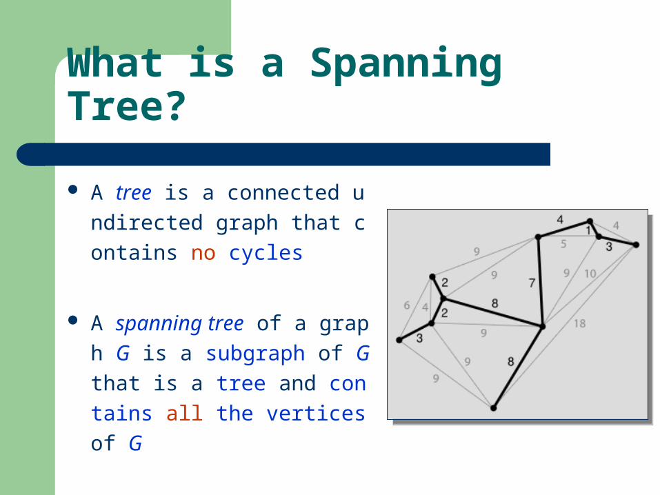
What is a Spanning Tree?
A tree is a connected undirected graph that contains no cycles
A spanning tree of a graph G is a subgraph of G that is a tree and contains all the vertices of G
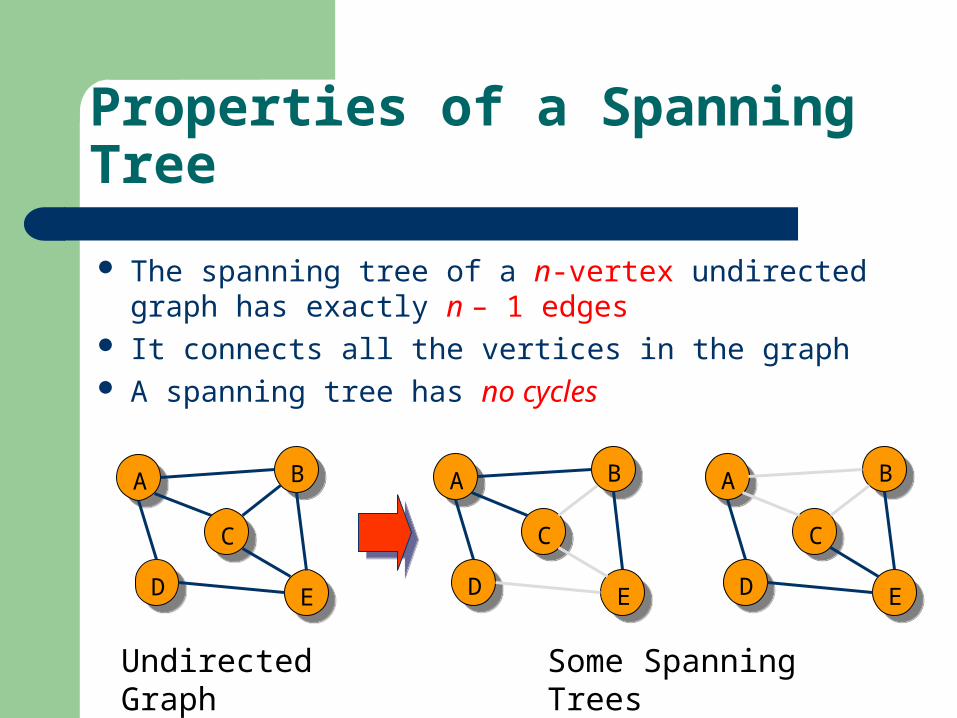
Properties of a Spanning Tree
The spanning tree of a n-vertex undirected graph has exactly n – 1 edges
It connects all the vertices in the graph A spanning tree has no cycles
Undirected Graph
Some Spanning Trees
AA
EEDD
CC
BB AA
EEDD
CC
BB AA
EEDD
CC
BB
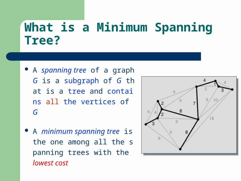
What is a Minimum Spanning Tree?
A spanning tree of a graph G is a subgraph of G that is a tree and contains all the vertices of G
A minimum spanning tree is the one among all the spanning trees with the lowest cost

Applications of MSTs
Computer Networks– To find how to connect a set of computers
using the minimum amount of wire
Shipping/Airplane Lines– To find the fastest way between locations
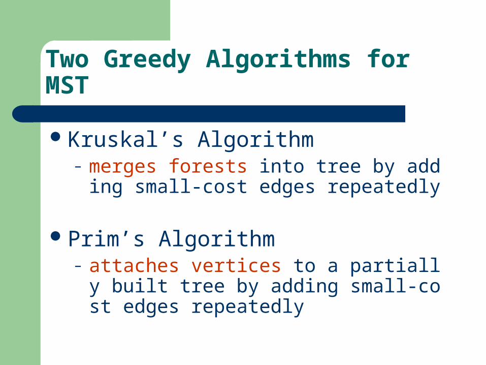
Two Greedy Algorithms for MST
Kruskal’s Algorithm– merges forests into tree by adding small-
cost edges repeatedly
Prim’s Algorithm– attaches vertices to a partially built tree
by adding small-cost edges repeatedly
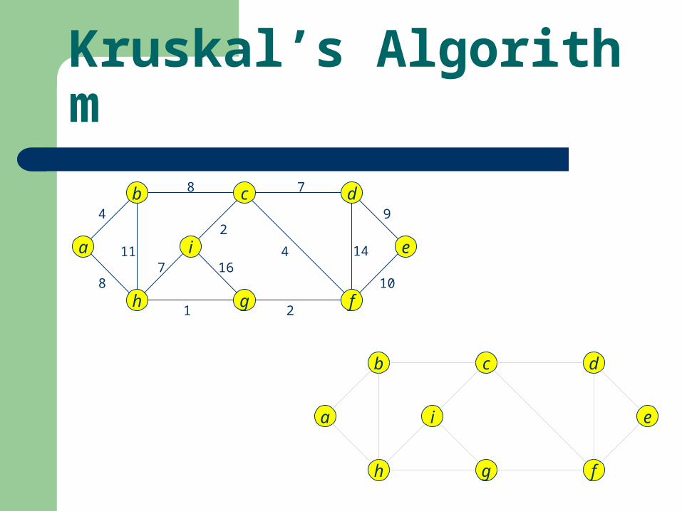
Kruskal’s Algorithm
a
b
h
i
c
g
e
d
f
a
b
h
i
c
g
e
d
f
4
8 7
9
10
144
2
21
711
816
Kruskal’s Algorithm
a
b
h
i
c
g
e
d
f
4
8 7
9
10
144
2
21
711
8
a
b
h
i
c
g
e
d
f
16
Kruskal’s Algorithm
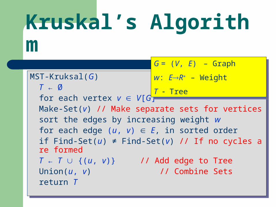
MST-Kruksal(G)T ← Øfor each vertex v V[G]
Make-Set(v) // Make separate sets for verticessort the edges by increasing weight wfor each edge (u, v) E, in sorted order
if Find-Set(u) ≠ Find-Set(v) // If no cycles are formedT ← T {(u, v)} // Add edge to TreeUnion(u, v) // Combine Sets
return T
MST-Kruksal(G)T ← Øfor each vertex v V[G]
Make-Set(v) // Make separate sets for verticessort the edges by increasing weight wfor each edge (u, v) E, in sorted order
if Find-Set(u) ≠ Find-Set(v) // If no cycles are formedT ← T {(u, v)} // Add edge to TreeUnion(u, v) // Combine Sets
return T
G = (V, E) – Graph
w: ER+ – Weight
T Tree
G = (V, E) – Graph
w: ER+ – Weight
T Tree
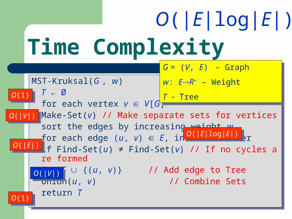
Time Complexity
MST-Kruksal(G , w)T ← Øfor each vertex v V[G]
Make-Set(v) // Make separate sets for verticessort the edges by increasing weight wfor each edge (u, v) E, in sorted order
if Find-Set(u) ≠ Find-Set(v) // If no cycles are formedT ← T {(u, v)} // Add edge to TreeUnion(u, v) // Combine Sets
return T
MST-Kruksal(G , w)T ← Øfor each vertex v V[G]
Make-Set(v) // Make separate sets for verticessort the edges by increasing weight wfor each edge (u, v) E, in sorted order
if Find-Set(u) ≠ Find-Set(v) // If no cycles are formedT ← T {(u, v)} // Add edge to TreeUnion(u, v) // Combine Sets
return T
G = (V, E) – Graph
w: ER+ – Weight
T Tree
G = (V, E) – Graph
w: ER+ – Weight
T TreeO(1)O(1)
O(|V|)O(|V|)
O(|E|)O(|E|)
O(|V|)O(|V|)
O(1)O(1)
O(|E|log|E|)
O(|E|log|E|)O(|E|log|E|)
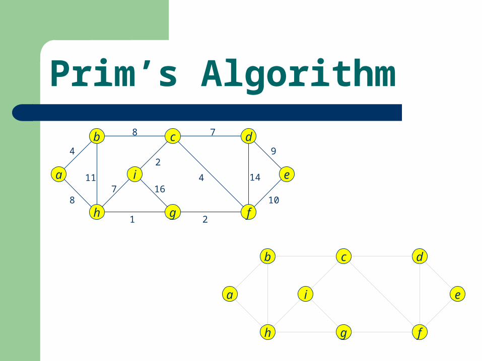
Prim’s Algorithm
a
b
h
i
c
g
e
d
f
a
b
h
i
c
g
e
d
f
4
8 7
9
10
144
2
21
711
816
Prim’s Algorithm
a
b
h
i
c
g
e
d
f
4
8 7
9
10
144
2
21
711
8
a
b
h
i
c
g
e
d
f
a
a
b
b
c
c
i
i
16
f
f
g
g
h
h
d
d
e
e
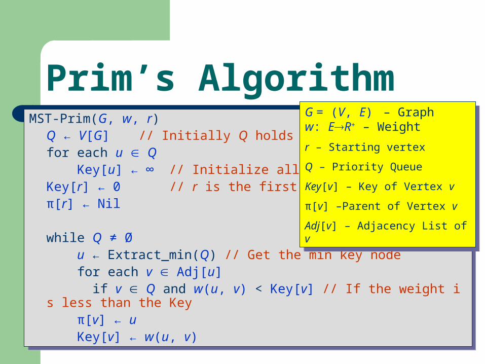
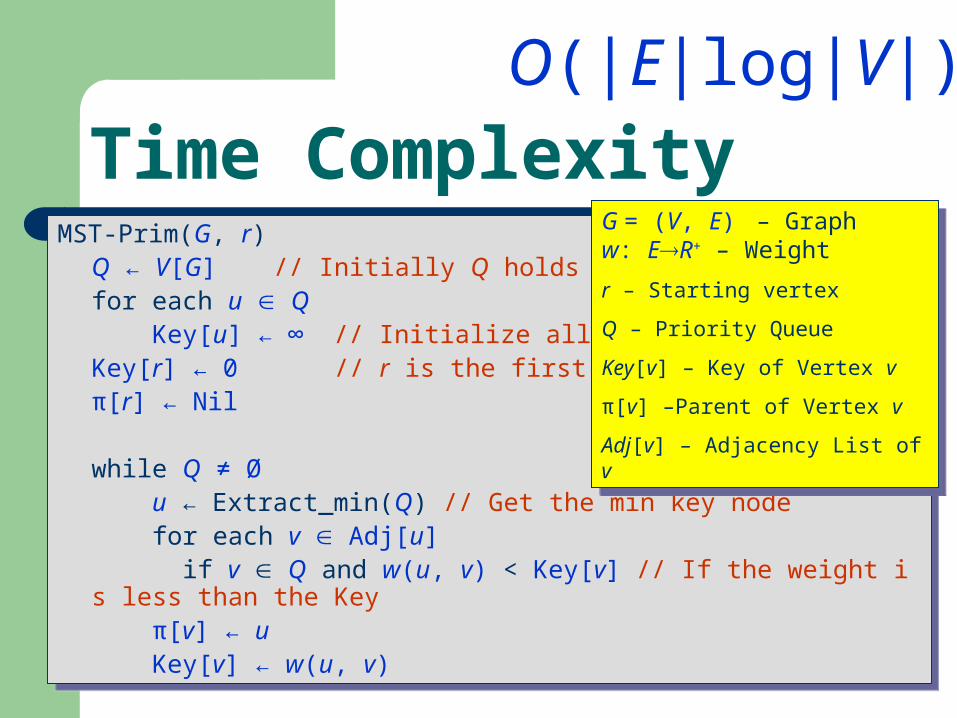
Prim’s AlgorithmMST-Prim(G, w, r)
Q ← V[G] // Initially Q holds all verticesfor each u Q Key[u] ← ∞ // Initialize all Keys to ∞ Key[r] ← 0 // r is the first tree node π[r] ← Nil
while Q ≠ Ø u ← Extract_min(Q) // Get the min key node for each v Adj[u] if v Q and w(u, v) < Key[v] // If the weight is less than the Key
π[v] ← u Key[v] ← w(u, v)
MST-Prim(G, w, r)Q ← V[G] // Initially Q holds all verticesfor each u Q Key[u] ← ∞ // Initialize all Keys to ∞ Key[r] ← 0 // r is the first tree node π[r] ← Nil
while Q ≠ Ø u ← Extract_min(Q) // Get the min key node for each v Adj[u] if v Q and w(u, v) < Key[v] // If the weight is less than the Key
π[v] ← u Key[v] ← w(u, v)
G = (V, E) – Graphw: ER+ – Weight
r – Starting vertex
Q – Priority Queue
Key[v] – Key of Vertex v
π[v] –Parent of Vertex v
Adj[v] – Adjacency List of v
G = (V, E) – Graphw: ER+ – Weight
r – Starting vertex
Q – Priority Queue
Key[v] – Key of Vertex v
π[v] –Parent of Vertex v
Adj[v] – Adjacency List of v
MST-Prim(G, r)Q ← V[G] // Initially Q holds all verticesfor each u Q Key[u] ← ∞ // Initialize all Keys to ∞ Key[r] ← 0 // r is the first tree node π[r] ← Nil
while Q ≠ Ø u ← Extract_min(Q) // Get the min key node for each v Adj[u] if v Q and w(u, v) < Key[v] // If the weight is less than the Key
π[v] ← u Key[v] ← w(u, v)
Time ComplexityO(|E|log|V|)
G = (V, E) – Graphw: ER+ – Weight
r – Starting vertex
Q – Priority Queue
Key[v] – Key of Vertex v
π[v] –Parent of Vertex v
Adj[v] – Adjacency List of v
G = (V, E) – Graphw: ER+ – Weight
r – Starting vertex
Q – Priority Queue
Key[v] – Key of Vertex v
π[v] –Parent of Vertex v
Adj[v] – Adjacency List of v
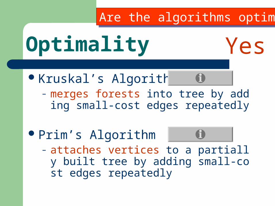
Optimality
Kruskal’s Algorithm– merges forests into tree by adding small-
cost edges repeatedly
Prim’s Algorithm– attaches vertices to a partially built tree
by adding small-cost edges repeatedly
Are the algorithms optimal?Are the algorithms optimal?
Yes
Lecture 1: The Greedy Method
Shortest Path Problem
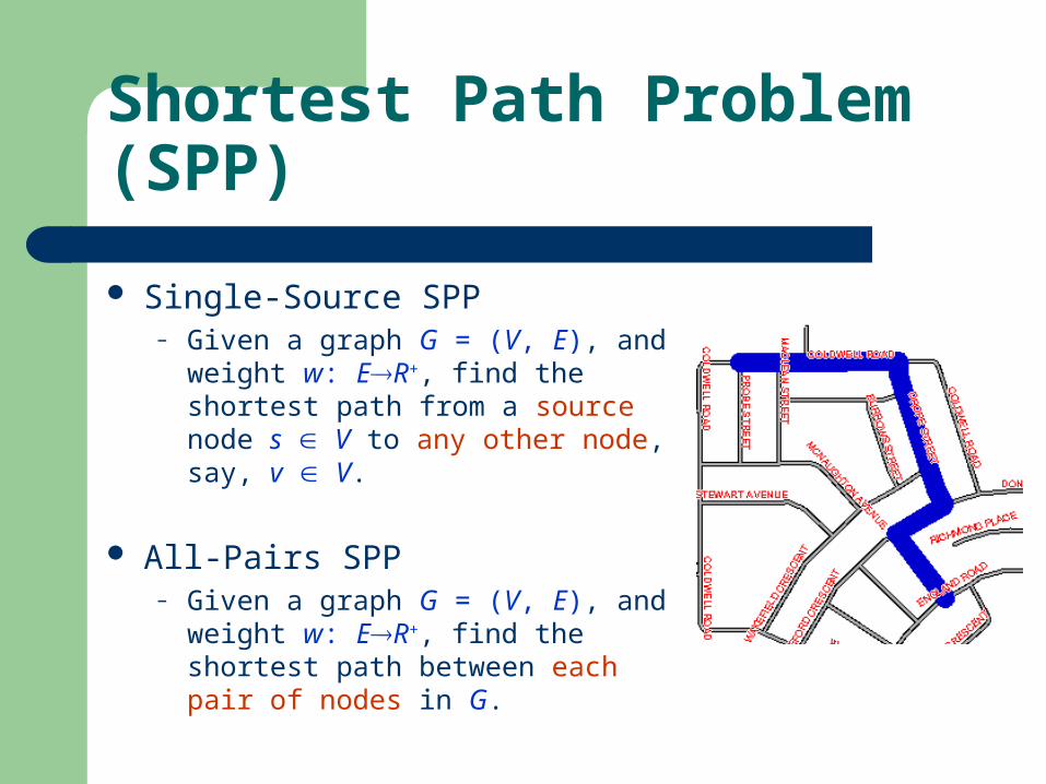
Shortest Path Problem (SPP)
Single-Source SPP– Given a graph G = (V, E), and
weight w: ER+, find the shortest path from a source node s V to any other node, say, v V.
All-Pairs SPP– Given a graph G = (V, E), and
weight w: ER+, find the shortest path between each pair of nodes in G.
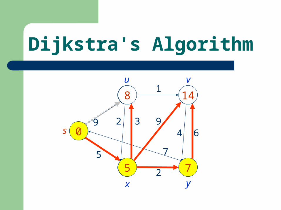
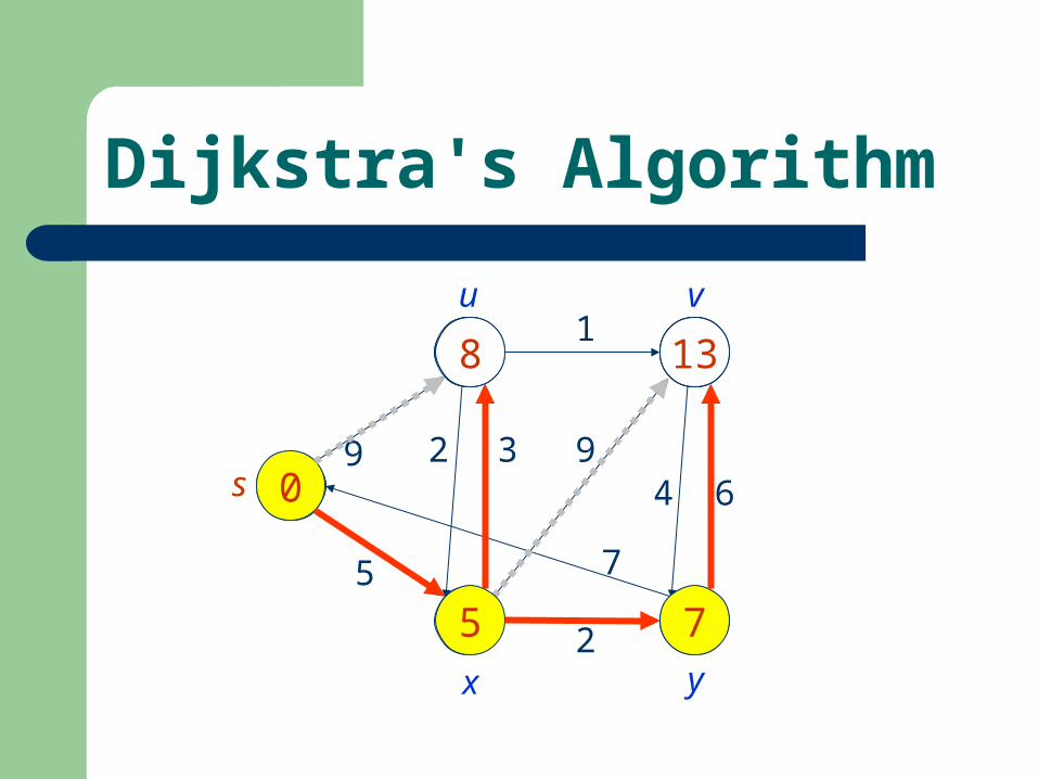
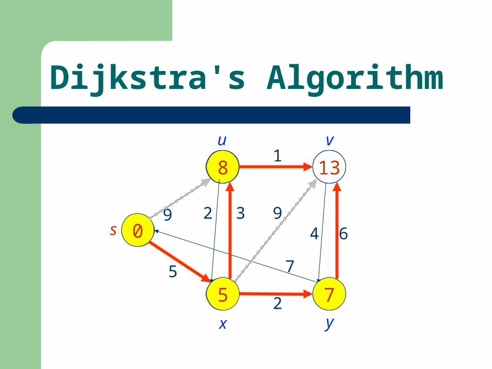
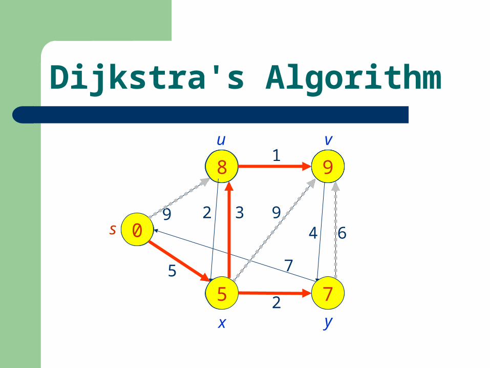
Dijkstra's Algorithm
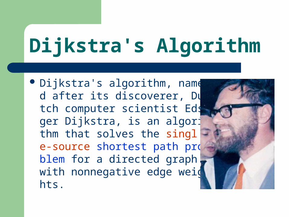
Dijkstra's algorithm, named after its discoverer, Dutch computer scientist Edsger Dijkstra, is an algorithm that solves the single-source shortest path problem for a directed graph with nonnegative edge weights.
Dijkstra's Algorithm
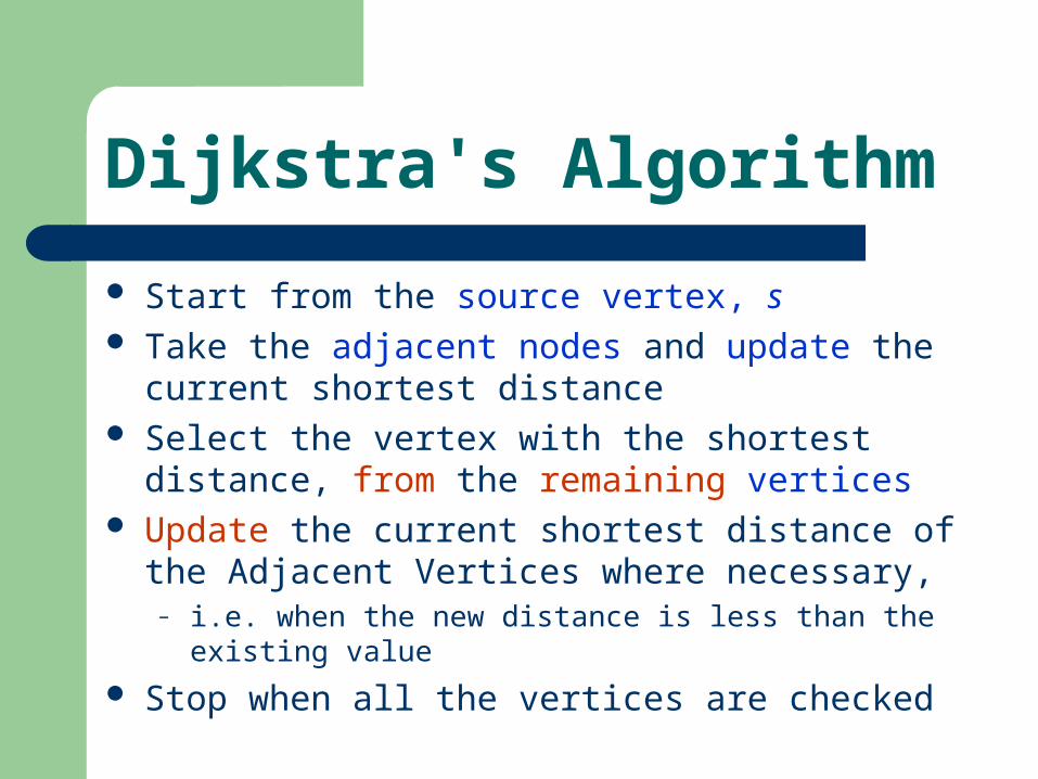
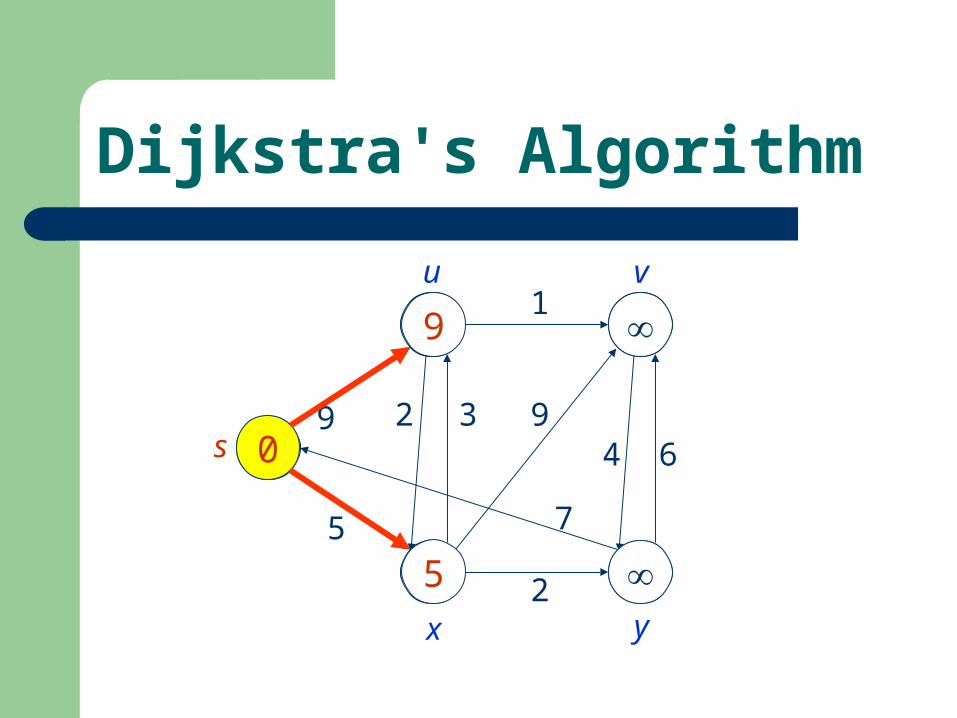
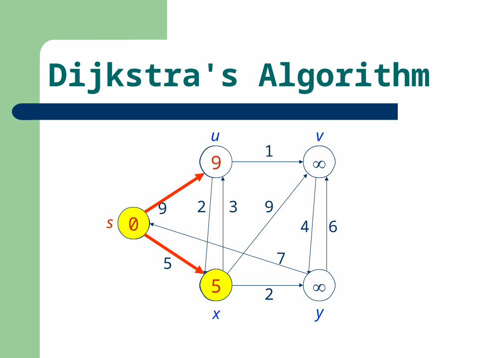
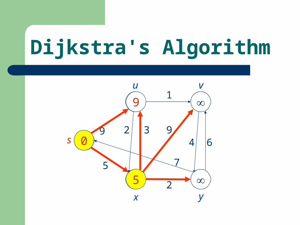
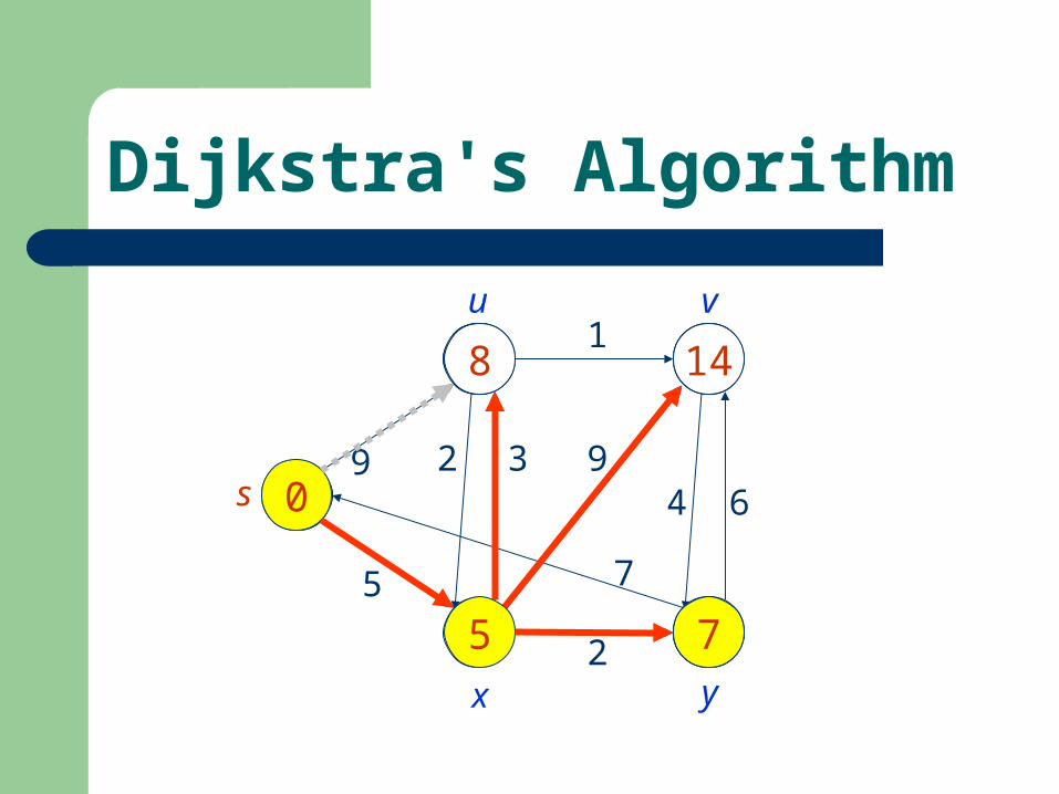
Start from the source vertex, s Take the adjacent nodes and update the
current shortest distance Select the vertex with the shortest distance,
from the remaining vertices Update the current shortest distance of the
Adjacent Vertices where necessary,– i.e. when the new distance is less than the existing
value Stop when all the vertices are checked
Dijkstra's Algorithm

Dijkstra's Algorithm
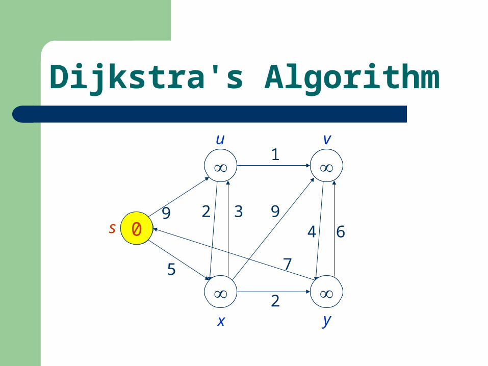
0
s
u v
x y
92 3
1
5
2
94 6
7

Dijkstra's Algorithm
0
s
u v
x y
92 3
1
5
2
94 6
7
Dijkstra's Algorithm
0
s
u v
x y
92 3
1
5
2
94 6
7
0
Dijkstra's Algorithm
0
s
u v
x y
92 3
1
5
2
94 6
7
0
9
5
Dijkstra's Algorithm
0
s
u v
x y
92 3
1
5
2
94 6
7
0
9
55
Dijkstra's Algorithm
0
s
u v
x y
92 3
1
5
2
94 6
7
0
9
5

Dijkstra's Algorithm
0
s
u v
x y
92 3
1
5
2
94 6
7
0
9
5
8 14
7
Dijkstra's Algorithm
0
s
u v
x y
92 3
1
5
2
94 6
7
0
9
5
8 14
77
Dijkstra's Algorithm
0
s
u v
x y
92 3
1
5
2
94 6
7
0
9
5
8 14
7
Dijkstra's Algorithm
0
s
u v
x y
92 3
1
5
2
94 6
7
0
9
5
8 14
7
13

Dijkstra's Algorithm
0
s
u v
x y
92 3
1
5
2
94 6
7
0
9
5
8 14
7
138
8
Dijkstra's Algorithm
0
s
u v
x y
92 3
1
5
2
94 6
7
0
5
14
7
13

8
Dijkstra's Algorithm
0
s
u v
x y
92 3
1
5
2
94 6
7
0
5
14
7
139
8
Dijkstra's Algorithm
0
s
u v
x y
92 3
1
5
2
94 6
7
0
5
14
7
1399
Dijkstra's Algorithm
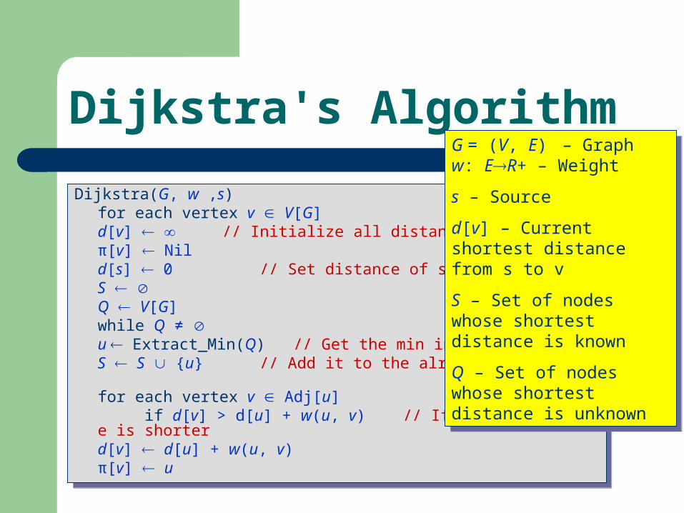
Dijkstra(G, w ,s)for each vertex v V[G]
d[v] // Initialize all distances to π[v] Nil
d[s] 0 // Set distance of source to 0 S Q V[G]while Q ≠
u Extract_Min(Q) // Get the min in Q S S {u} // Add it to the already known list for each vertex v Adj[u] if d[v] > d[u] + w(u, v) // If the new distance is shorter
d[v] d[u] + w(u, v) π[v] u
G = (V, E) – Graphw: ER+ – Weight
s – Source
d[v] – Current shortest distance from s to v
S – Set of nodes whose shortest distance is known
Q – Set of nodes whose shortest distance is unknown
G = (V, E) – Graphw: ER+ – Weight
s – Source
d[v] – Current shortest distance from s to v
S – Set of nodes whose shortest distance is known
Q – Set of nodes whose shortest distance is unknown
Lecture 1: The Greedy Method
Huffman Codes
Huffman Codes
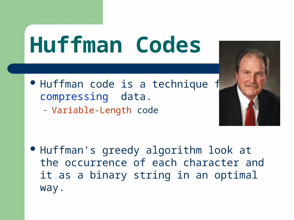
Huffman code is a technique for compressing data.– Variable-Length code
Huffman's greedy algorithm look at the occurrence of each character and it as a binary string in an optimal way.
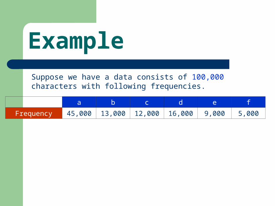
Example
a b c d e f
Frequency 45,000 13,000 12,000 16,000 9,000 5,000
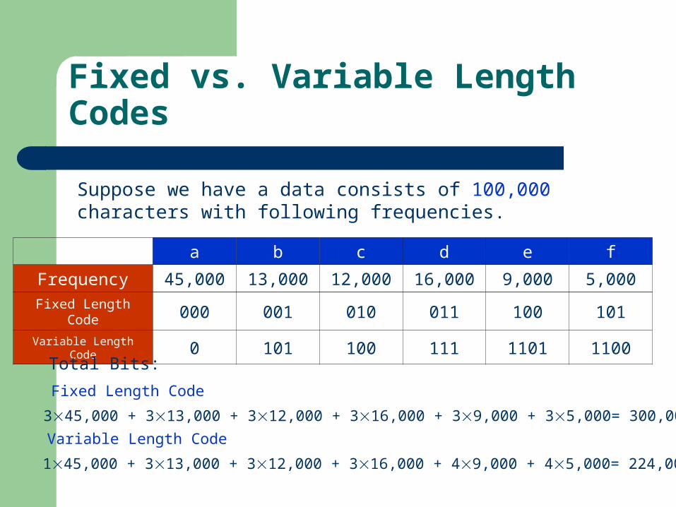
Suppose we have a data consists of 100,000 characters with following frequencies.
Fixed vs. Variable Length Codes
a b c d e f
Frequency 45,000 13,000 12,000 16,000 9,000 5,000
Suppose we have a data consists of 100,000 characters with following frequencies.
Fixed Length Code 000 001 010 011 100 101
Variable Length Code 0 101 100 111 1101 1100
Total Bits:
Fixed Length Code
Variable Length Code
145,000 + 313,000 + 312,000 + 316,000 + 49,000 + 45,000= 224,000
345,000 + 313,000 + 312,000 + 316,000 + 39,000 + 35,000= 300,000
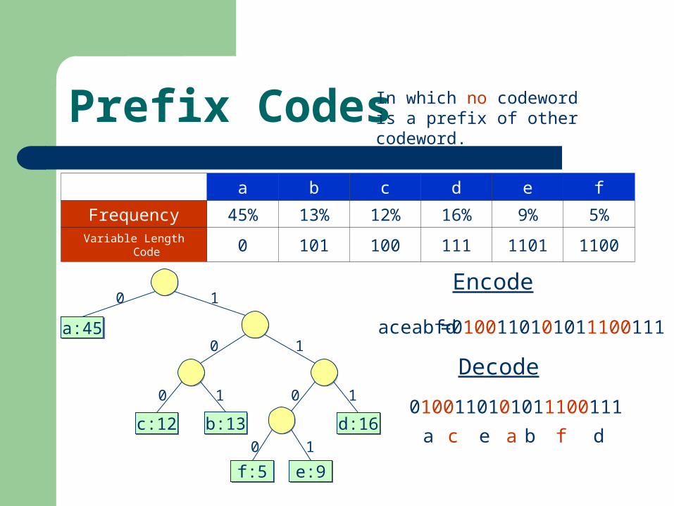
Prefix Codes
a b c d e f
Frequency 45% 13% 12% 16% 9% 5%
Variable Length Code 0 101 100 111 1101 1100
In which no codeword is a prefix of other codeword.
a:45a:45
c:12c:12 b:13b:13 d:16d:16
f:5f:5 e:9e:9
0 1
0 1
0 1 0 1
0 1
Encode
Decode
aceabfd=0100110101011100111
0100110101011100111
a c e a b f d
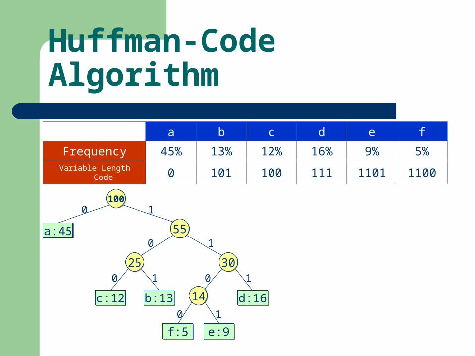
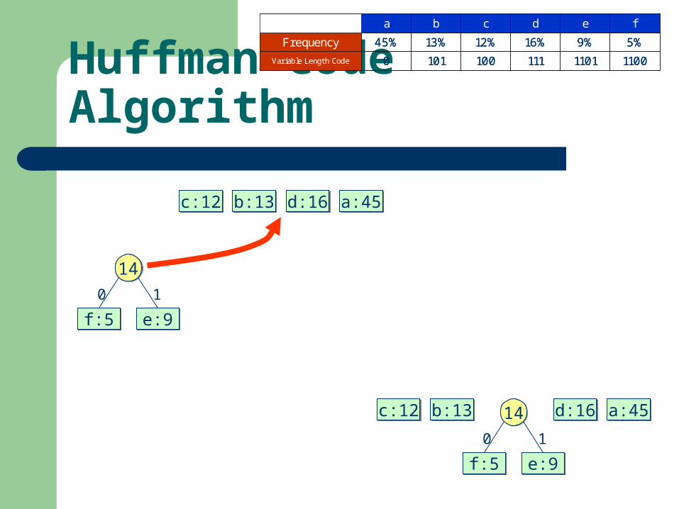
Huffman-Code Algorithm
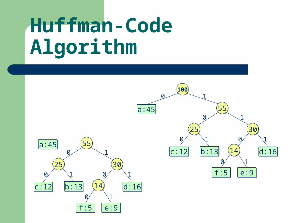
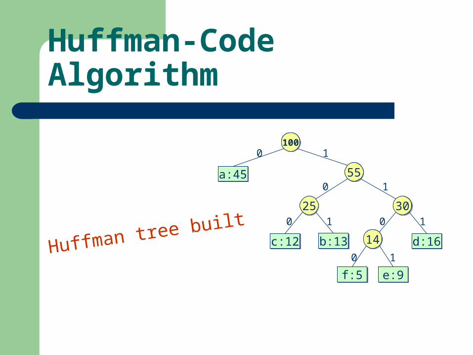
a b c d e f
Frequency 45% 13% 12% 16% 9% 5%
Variable Length Code 0 101 100 111 1101 1100
a:45a:45
c:12c:12 b:13b:13 d:16d:16
f:5f:5 e:9e:9
0 1
0 1
0 1 0 1
0 1
100
14
3025
55
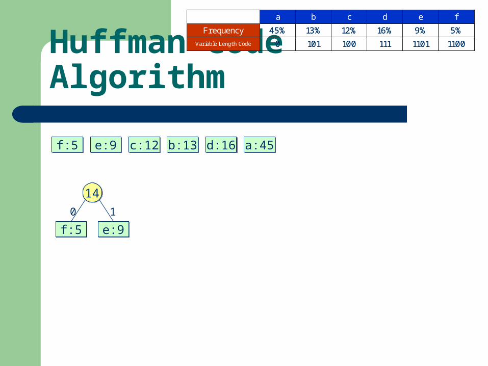
Huffman-Code Algorithm
a:45a:45c:12c:12 b:13b:13 d:16d:16f:5f:5 e:9e:9
5%9%16%12%13%45%Frequency
110011011111001010Variable Length Code
fedcba
5%9%16%12%13%45%Frequency
110011011111001010Variable Length Code
fedcba
f:5f:5 e:9e:9
0 1
14
Huffman-Code Algorithm
a:45a:45c:12c:12 b:13b:13 d:16d:16f:5f:5 e:9e:9
5%9%16%12%13%45%Frequency
110011011111001010Variable Length Code
fedcba
5%9%16%12%13%45%Frequency
110011011111001010Variable Length Code
fedcba
f:5f:5 e:9e:9
0 1
14
a:45a:45c:12c:12 b:13b:13 d:16d:16
f:5f:5 e:9e:9
0 1
14
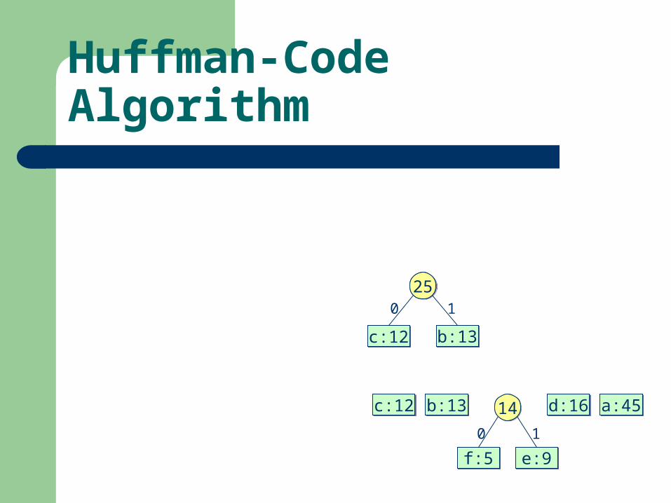
Huffman-Code Algorithm
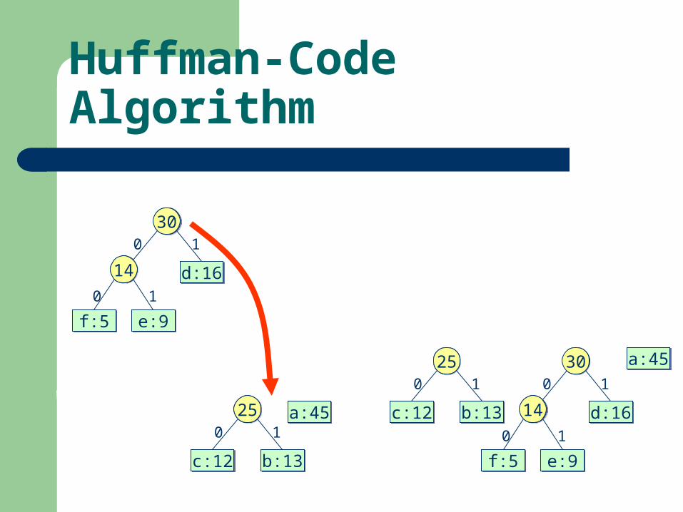
a:45a:45c:12c:12 b:13b:13 d:16d:16
f:5f:5 e:9e:9
0 1
14
c:12c:12 b:13b:13
0 125
Huffman-Code Algorithm
a:45a:45c:12c:12 b:13b:13 d:16d:16
f:5f:5 e:9e:9
0 1
14
c:12c:12 b:13b:13
0 125
a:45a:45d:16d:16
f:5f:5 e:9e:9
0 1
14
c:12c:12 b:13b:13
0 125
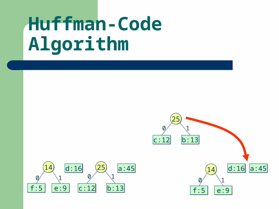
Huffman-Code Algorithm
a:45a:45d:16d:16
f:5f:5 e:9e:9
0 1
14
c:12c:12 b:13b:13
0 125
d:16d:16
0 1
f:5f:5 e:9e:9
0 1
14
30
Huffman-Code Algorithm
a:45a:45d:16d:16
f:5f:5 e:9e:9
0 1
14
c:12c:12 b:13b:13
0 125
d:16d:16
0 1
f:5f:5 e:9e:9
0 1
14
30
a:45a:45
c:12c:12 b:13b:13
0 125
d:16d:16
0 1
f:5f:5 e:9e:9
0 1
14
30
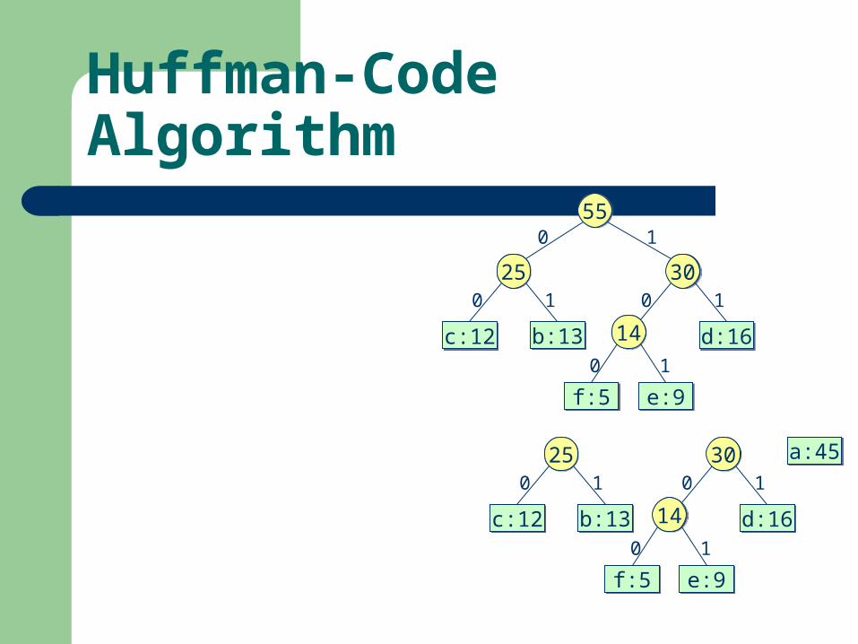
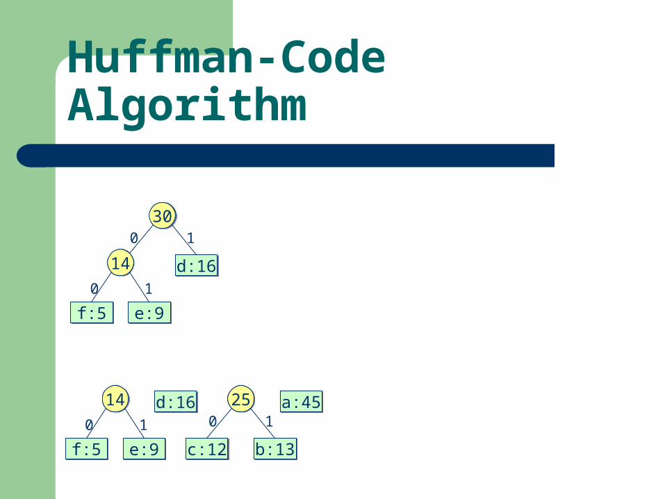
Huffman-Code Algorithm
a:45a:45
c:12c:12 b:13b:13
0 125
d:16d:16
0 1
f:5f:5 e:9e:9
0 1
14
30
0 1
d:16d:16
0 1
f:5f:5 e:9e:9
0 1
14
30
c:12c:12 b:13b:13
0 125
55
Huffman-Code Algorithm
a:45a:45
c:12c:12 b:13b:13
0 125
d:16d:16
0 1
f:5f:5 e:9e:9
0 1
14
30
0 1
d:16d:16
0 1
f:5f:5 e:9e:9
0 1
14
30
c:12c:12 b:13b:13
0 125
55
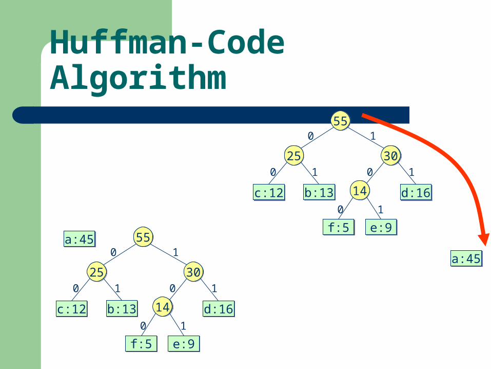
a:45a:450 1
d:16d:16
0 1
f:5f:5 e:9e:9
0 1
14
30
c:12c:12 b:13b:13
0 125
55
Huffman-Code Algorithm
c:12c:12 b:13b:13
0 125
d:16d:16
0 1
f:5f:5 e:9e:9
0 1
14
30
a:45a:450 1
d:16d:16
0 1
f:5f:5 e:9e:9
0 1
14
30
c:12c:12 b:13b:13
0 125
55
a:45a:45
0 1100
0 1
d:16d:16
0 1
f:5f:5 e:9e:9
0 1
14
30
c:12c:12 b:13b:13
0 125
55
Huffman-Code Algorithm
c:12c:12 b:13b:13
0 125
d:16d:16
0 1
f:5f:5 e:9e:9
0 1
14
30
a:45a:450 1
d:16d:16
0 1
f:5f:5 e:9e:9
0 1
14
30
c:12c:12 b:13b:13
0 125
55
a:45a:45
0 1100
0 1
d:16d:16
0 1
f:5f:5 e:9e:9
0 1
14
30
c:12c:12 b:13b:13
0 125
55
Huffman tree built
Huffman-Code Algorithm
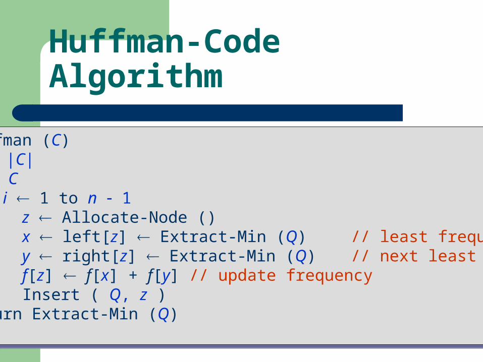
Huffman (C)n |C| Q C for i 1 to n 1 z Allocate-Node () x left[z] Extract-Min (Q) // least frequent y right[z] Extract-Min (Q) // next least f[z] f[x] + f[y] // update frequency Insert ( Q, z ) return Extract-Min (Q)
Huffman (C)n |C| Q C for i 1 to n 1 z Allocate-Node () x left[z] Extract-Min (Q) // least frequent y right[z] Extract-Min (Q) // next least f[z] f[x] + f[y] // update frequency Insert ( Q, z ) return Extract-Min (Q)

Optimality
Exercise