BBM 205 Discrete MathematicsHacettepe University

Lecture 13a: Probabilistic Method

Lale Özkahya

Resources:Kenneth Rosen, �Discrete Mathematics and App.�

http://www.math.caltech.edu/ 2015-16/2term/ma006b

2/4/2016

2

Independent Events

Two events 𝐴, 𝐵 ⊂ Ω are independent ifPr 𝐴 ∩ 𝐵 = Pr 𝑎 ⋅ Pr 𝑏 .

Example. We flip two fair coins.

◦ Let 𝜔𝑖,𝑗 be the elementary event that coin A

landed on 𝑖 and coin 𝐵 on 𝑗, where 𝑖, 𝑗 ∈ {ℎ, 𝑡}. Each of the four events has a probability of 0.25.

◦ The event where coin 𝐴 lands on heads is

𝑎 = 𝜔ℎ,𝑡, 𝜔ℎ,ℎ . For 𝐵 it is 𝑏 = 𝜔𝑡,ℎ, 𝜔ℎ,ℎ .

◦ The events are independent since

Pr 𝑎 and 𝑏 = Pr 𝜔ℎ,ℎ = 0.25 = Pr 𝑎 ⋅ Pr 𝑏 .

(Discrete) Uniform Distribution

In a uniform distribution we have a set Ωof elementary events, each occurring with

probability 1

Ω.

◦ For example, when flipping a fair die, we have a uniform distribution over the six possible results.

2/4/2016

3

Union Bound

For any two events 𝐴, 𝐵, we havePr 𝐴 ∪ 𝐵 = Pr 𝐴 + Pr 𝐵 − Pr 𝐴 ∩ 𝐵 .

This immediately implies that Pr 𝐴 ∪ 𝐵 ≤ Pr 𝐴 + Pr 𝐵 ,

where equality holds iff 𝐴, 𝐵 are disjoint.

Union bound. For any finite set of events 𝐴1, … , 𝐴𝑘, we have

Pr ∪𝑖 𝐴𝑖 ≤

𝑖

Pr 𝐴𝑖 .

Recall: Ramsey Numbers

𝑅 𝑝, 𝑝 is the smallest number 𝑛 such that each blue-red edge coloring of 𝐾𝑛contains a monochromatic 𝐾𝑝.

Theorem. 𝑅 𝑝, 𝑝 > 2𝑝/2.

◦ We proved this in a previous class.

◦ Now we provide another proof, using probability.

2/4/2016

4

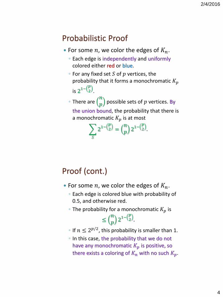
Probabilistic Proof

For some 𝑛, we color the edges of 𝐾𝑛.

◦ Each edge is independently and uniformlycolored either red or blue.

◦ For any fixed set 𝑆 of 𝑝 vertices, the probability that it forms a monochromatic 𝐾𝑝

is 21−𝑝2 .

◦ There are 𝑛𝑝 possible sets of 𝑝 vertices. By

the union bound, the probability that there is a monochromatic 𝐾𝑝 is at most

𝑆

21−𝑝2 =𝑛𝑝 21−𝑝2 .

Proof (cont.)

For some 𝑛, we color the edges of 𝐾𝑛.

◦ Each edge is colored blue with probability of 0.5, and otherwise red.

◦ The probability for a monochromatic 𝐾𝑝 is

≤𝑛𝑝 21−𝑝2 .

◦ If 𝑛 ≤ 2𝑝/2, this probability is smaller than 1.

◦ In this case, the probability that we do not have any monochromatic 𝐾𝑝 is positive, so

there exists a coloring of 𝐾𝑛 with no such 𝐾𝑝.

2/4/2016

5

Non-Constructive Proofs

We proved that there exists a coloring of 𝐾𝑛 with no monochromatic 𝐾𝑝, but we

have no idea how to find this coloring.

Such a proof is called non-constructive.

The probabilistic method often proves the existence of objects with surprising properties, but we still have no idea how they look like.

A Tournament

We have 𝑛 people competing in thumb wrestling.

◦ Every pair of contestants compete once.

◦ How can we decide who the overall winner is?

We build a directed graph:

◦ A vertex for every participant.

◦ An edge between every two vertices, directed from the winner to the loser.

◦ An orientation of 𝐾𝑛 is called a tournament.

2/4/2016

6

The King of the Tournament

The winner can be the vertex with the maximum outdegree (the contestant winning the largest number of matches), but it might not be unique.

A king is a contestant 𝑥 such that for every other contestant 𝑦 either 𝑥 → 𝑦 or there exists 𝑧 such that 𝑥 → 𝑧 → 𝑦.

Theorem. Every tournament has a king.

Proof

𝐷+(𝑣) – the number of vertices reachable from 𝑣 by a path of length ≤ 2.

Let 𝑣 be a vertex that maximizes 𝐷+ 𝑣 .

◦ Assume for contradiction that 𝑣 is not a king.

◦ Then there exists 𝑢 such that 𝑢 → 𝑣 and there is no path of length two from 𝑣 to 𝑢.

◦ That is, for every 𝑤 such that 𝑣 → 𝑤, we also have 𝑢 → 𝑤.

◦ But this implies that 𝐷+ 𝑢 ≥ 𝐷+ 𝑣 + 1, contradicting the maximality of 𝑣!

2/4/2016

7

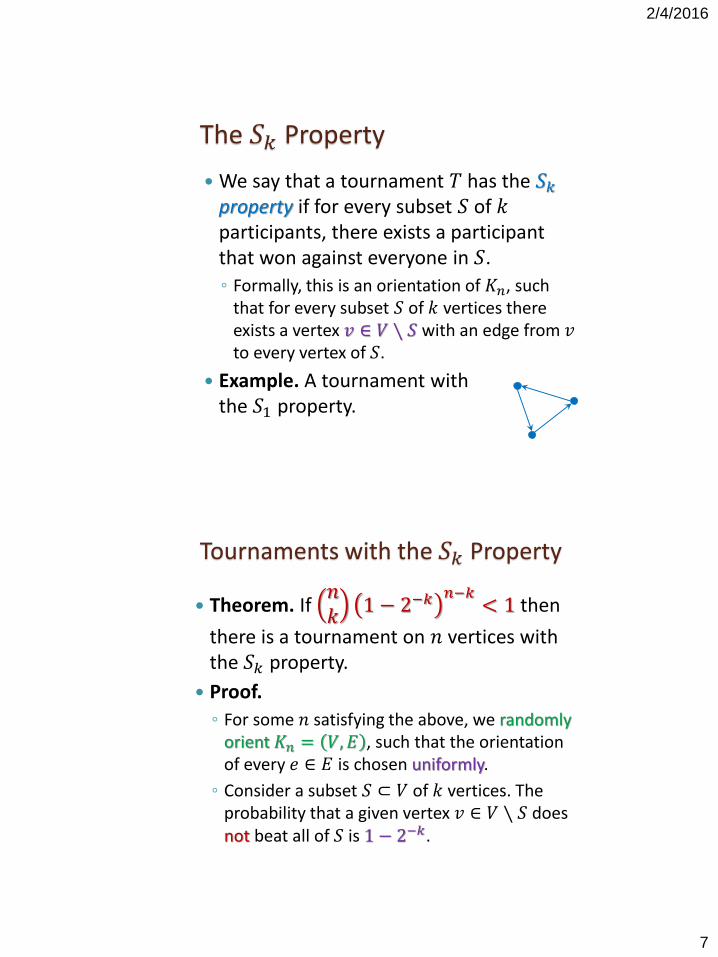
The 𝑆𝑘 Property

We say that a tournament 𝑇 has the 𝑆𝑘property if for every subset 𝑆 of 𝑘participants, there exists a participant that won against everyone in 𝑆.

◦ Formally, this is an orientation of 𝐾𝑛, such that for every subset 𝑆 of 𝑘 vertices there exists a vertex 𝑣 ∈ 𝑉 ∖ 𝑆 with an edge from 𝑣to every vertex of 𝑆.

Example. A tournament with the 𝑆1 property.

Tournaments with the 𝑆𝑘 Property

Theorem. If 𝑛𝑘1 − 2−𝑘

𝑛−𝑘< 1 then

there is a tournament on 𝑛 vertices with the 𝑆𝑘 property.

Proof.

◦ For some 𝑛 satisfying the above, we randomly orient 𝐾𝑛 = 𝑉, 𝐸 , such that the orientation of every 𝑒 ∈ 𝐸 is chosen uniformly.

◦ Consider a subset 𝑆 ⊂ 𝑉 of 𝑘 vertices. The probability that a given vertex 𝑣 ∈ 𝑉 ∖ 𝑆 does not beat all of 𝑆 is 1 − 2−𝑘.

2/4/2016

8

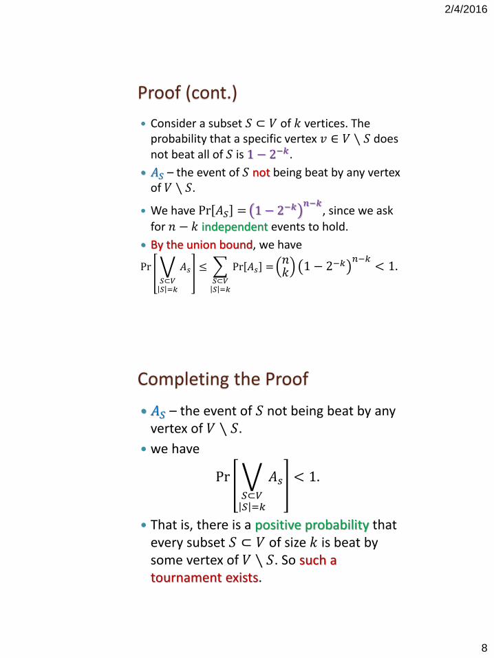
Proof (cont.)

Consider a subset 𝑆 ⊂ 𝑉 of 𝑘 vertices. The probability that a specific vertex 𝑣 ∈ 𝑉 ∖ 𝑆 does not beat all of 𝑆 is 1 − 2−𝑘.

𝐴𝑆 – the event of 𝑆 not being beat by any vertex of 𝑉 ∖ 𝑆.

We have Pr 𝐴𝑆 = 1 − 2−𝑘 𝑛−𝑘, since we ask

for 𝑛 − 𝑘 independent events to hold.

By the union bound, we have

Pr 𝑆⊂𝑉𝑆 =𝑘

𝐴𝑠 ≤ 𝑆⊂𝑉𝑆 =𝑘

Pr 𝐴𝑠 =𝑛𝑘 1 − 2

−𝑘 𝑛−𝑘 < 1.

Completing the Proof

𝐴𝑆 – the event of 𝑆 not being beat by any vertex of 𝑉 ∖ 𝑆.

we have

Pr 𝑆⊂𝑉𝑆 =𝑘

𝐴𝑠 < 1.

That is, there is a positive probability that every subset 𝑆 ⊂ 𝑉 of size 𝑘 is beat by some vertex of 𝑉 ∖ 𝑆. So such a tournament exists.

2/4/2016

9

Which NBA Player is Related to Mathematics?

Michael Jordan

LeBron James

Shaquille O'Neal

Random Variables

A random variable is a function from the set of possible events to ℝ.

Example. Say that we flip five coins.

◦ We can define the random variable 𝑋 to be the number of coins that landed on heads.

◦ We can define the random variable 𝑌 to be the percentage of heads in the tosses.

◦ Notice that 𝑌 = 20𝑋.

2/4/2016

10

Indicator Random Variables

An indicator random variable is a random variable 𝑋 that is either 0 or 1, according to whether some event happens or not.

Example. We toss a fair die.

◦ We can define the six indicator variable 𝑋1, … , 𝑋6 such that 𝑋𝑖 = 1 iff the result of the roll is 𝑖.

Expectation

The expectation of a random variable 𝑋 is

𝐸 𝑋 =

𝜔∈Ω

𝑋 𝜔 Pr 𝜔 .

◦ Intuitively, 𝐸 𝑋 is the expected value of 𝑋 in the long-run average value when repeating the experiment 𝑋 represents.

2/4/2016

11

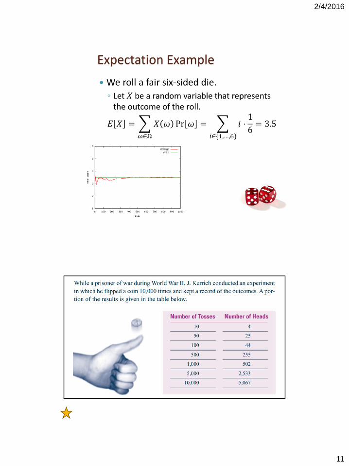
Expectation Example

We roll a fair six-sided die.

◦ Let 𝑋 be a random variable that represents the outcome of the roll.

𝐸 𝑋 =

𝜔∈Ω

𝑋 𝜔 Pr 𝜔 =

𝑖∈{1,…,6}

𝑖 ⋅1

6= 3.5

2/4/2016

12

Linearity of Expectation

If 𝑋 is a random variable, then 5𝑋 is a random variable with a value five times that of 𝑋

Lemma. Let 𝑋1, 𝑋2, … , 𝑋𝑘 be a collection set of random variables over the same discrete probability. Let 𝑐1, … , 𝑐𝑘 be constants. Then

𝐸 𝑐1𝑋1 + 𝑐2𝑋2 +⋯+ 𝑐𝑘𝑋𝑘 =

𝑖=1

𝑘

𝑐𝑖𝐸 𝑋𝑖 .

Fixed Elements in Permutations

Let 𝜎 be a uniformly chosen permutation of 1,2, … , 𝑛 .

◦ For 1 ≤ 𝑖 ≤ 𝑛, let 𝑋𝑖 be an indicator variable that is 1 if 𝑖 is fixed by 𝜎.

◦ 𝐸 𝑋𝑖 = Pr 𝜎 𝑖 = 𝑖 =𝑛−1 !

𝑛!=1

𝑛.

◦ Let 𝑋 be the number of fixed elements in 𝜎.

◦ We have 𝑋 = 𝑋1 +⋯+ 𝑋𝑛.

◦ By linearity of expectation

𝐸 𝑋 =

𝑖

𝐸 𝑋𝑖 = 𝑛 ⋅1

𝑛= 1.

2/4/2016

13

Hamiltonian Paths

Given a directed graph 𝐺 = 𝑉, 𝐸 , a Hamiltonian path is a path that visits every vertex of 𝑉 exactly once.

◦ Major problem in theoretical computer science: Does there exist a polynomial-time algorithm for finding whether a Hamiltonian path exists in a given graph.

Undirected Hamiltonian paths

Hamiltonian Paths in Tournaments

Theorem. There exists a tournament 𝑇with 𝑛 players that contains at least

𝑛! 2−(𝑛−1) Hamiltonian paths.

2/4/2016

14

Proof

We uniformly choose an orientation of the edges of 𝐾𝑛 to obtain a tournament 𝑇.

◦ There is a bijection between the possible Hamiltonian paths and the permutations of 1,2,… , 𝑛 . Every possible path defines a

unique permutation, according to the order in which it visits the vertices.

◦ For a permutation 𝜎, let 𝑋𝜎 be an indicator variable that is 1 if the path corresponding to 𝜎 exists in 𝑇.

◦ We have 𝐸 𝑋𝜎 = Pr 𝑋𝜎 = 1 = 2− 𝑛−1 .

We uniformly choose an orientation of the edges of 𝐾𝑛 to obtain a tournament 𝑇.

◦ For a permutation 𝜎, let 𝑋𝜎 be an indicator variable that is 1 if the path corresponding to 𝜎 exists 𝑇.

◦ We have 𝐸 𝑋𝜎 = Pr 𝑋𝜎 = 1 = 2−𝑛+1 .

◦ Let 𝑋 be a random variable of the number of Hamiltonian paths in 𝑇. Then 𝑋 = 𝜎𝑋𝜎.

𝐸 𝑋 = 𝐸

𝜎

𝑋𝜎 =

𝜎

𝐸 𝑋𝜎 = 𝑛! 2−𝑛+1.

◦ Since this is the expected number of paths in a uniformly chosen tournament, there must is a orientation with at least as many paths.

2/9/2016

2

Reminder: Indicator Random Variables An indicator random variable is a random

variable 𝑋 that is either 0 or 1, according to whether some event happens or not.

Example. We toss a die.

◦ We can define the six indicator variable 𝑋1, … , 𝑋6 such that 𝑋𝑖 = 1 iff the result of the roll is 𝑖.

Reminder: Expectation

The expectation of a random variable 𝑋 is

𝐸 𝑋 =

𝜔∈Ω

𝑋 𝜔 Pr 𝜔 .

◦ Intuitively, 𝐸 𝑋 is the expected value of 𝑋 in the long-run average value of repetitions of the experiment it represents.

2/9/2016

3

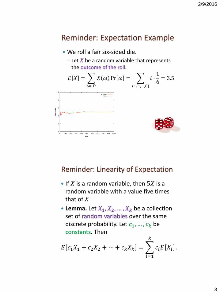
Reminder: Expectation Example

We roll a fair six-sided die.

◦ Let 𝑋 be a random variable that represents the outcome of the roll.

𝐸 𝑋 =

𝜔∈Ω

𝑋 𝜔 Pr 𝜔 =

𝑖∈{1,…,6}

𝑖 ⋅1

6= 3.5

Reminder: Linearity of Expectation

If 𝑋 is a random variable, then 5𝑋 is a random variable with a value five times that of 𝑋

Lemma. Let 𝑋1, 𝑋2, … , 𝑋𝑘 be a collection set of random variables over the same discrete probability. Let 𝑐1, … , 𝑐𝑘 be constants. Then

𝐸 𝑐1𝑋1 + 𝑐2𝑋2 +⋯+ 𝑐𝑘𝑋𝑘 =

𝑖=1

𝑘

𝑐𝑖𝐸 𝑋𝑖 .

2/9/2016

4

Independent Sets

Consider a graph 𝐺 = 𝑉, 𝐸 . An independent set in 𝐺 is a subset 𝑉′ ⊂ 𝑉such that there is no edge between any two vertices of 𝑉′.

Finding a maximum independent set in a graph is a major problem in theoretical computer science.

◦ No polynomial-time algorithm is known.

Warm Up

What are the sizes of the maximum independent sets in:

2 4

2/9/2016

5

Large Independent Sets

Theorem. A graph 𝐺 = (𝑉, 𝐸) has an independent set of size at least

𝑣∈𝑉

1

1 + deg 𝑣.

Proof. We uniformly choose an ordering for the vertices of 𝑉 = 𝑣1, … , 𝑣𝑛 .

◦ The set of vertices that appear before all of their neighbors is an independent set.

We uniformly choose an ordering for the vertices of 𝑉 = 𝑣1, … , 𝑣𝑛 .

◦ The set 𝑆 of vertices that appear before all of their neighbors is an independent set.

◦ 𝑋𝑖 - indicator that is 1 if 𝑣𝑖 ∈ 𝑆.

𝐸 𝑋𝑖 = Pr 𝑋𝑖 = 1 =1

1 + deg𝑣𝑖.

◦ 𝑋 – the random variable of the size of 𝑆.

𝐸 𝑋 = 𝐸

𝑖=1

𝑛

𝑋𝑖 =

𝑖=1

𝑛

𝐸 𝑋𝑖 =

𝑖=1

𝑛1

1 + deg 𝑣𝑖.

◦ There must exist an ordering for which |𝑆| has at least this value.

2/9/2016

6

Sum-free Sets

Consider a set 𝐴 of positive integers. We say that 𝐴 is sum-free if for every 𝑥, 𝑦 ∈ 𝐴, we have that 𝑥 + 𝑦 ∉ 𝐴(including the case where 𝑥 = 𝑦).

What are large sum-free subsets of 𝑆 = 1,2, … ,𝑁 ?

◦ We can take all of the odd numbers in 𝑆.

◦ We can take all of the numbers in 𝑆 of size larger than 𝑁/2.

Large Sum-Free Sets Always Exist

Theorem. For any set of positive integers 𝐴, there is a sum-free subset 𝐵 ⊆ 𝐴 of

size |𝐵| ≥1

3|𝐴|.

Proof. Consider a prime 𝑝 such that 𝑝 > 𝑎for every 𝑎 ∈ 𝐴.

◦ From now on, calculations are 𝑚𝑜𝑑 𝑝.

◦ Notice that if 𝐵 is sum-free 𝑚𝑜𝑑 𝑝, it is also sum-free under standard addition.

◦ Thus, it suffices to find a large set that is sum-free 𝑚𝑜𝑑 𝑝.

2/9/2016

7

Proof (cont.)

The calculations are 𝑚𝑜𝑑 𝑝.

The set 𝑆 = 𝑝/3 ,… , 2𝑝/3 is sum-free and 𝑆 ≥ 𝑝 − 1 /3.

We uniformly choose 𝑥 ∈ 1,2,… , 𝑝 − 1 and set 𝐴𝑥 = 𝑎 ∈ 𝐴 | 𝑎𝑥 ∈ 𝑆 .

Consider 𝑏, 𝑐 ∈ 𝐴𝑥. Since 𝑏𝑥, 𝑐𝑥 ∈ 𝑆, we have that 𝑏 + 𝑐 𝑥 = 𝑏𝑥 + 𝑐𝑥 ∉ 𝑆. Thus, 𝑏 + 𝑐 ∉ 𝐴𝑥, and 𝐴𝑥 is sum-free.

𝑋𝑎 – indicator that is 1 if 𝑎 ∈ 𝐴𝑥.

𝐸 𝐴𝑥 = 𝐸

𝑎∈𝐴

𝑋𝑎 =

𝑎∈𝐴

𝐸 𝑋𝑎 =

𝑎∈𝐴

Pr 𝑋𝑎 = 1 .

The set 𝑆 = 𝑝/3 ,… , 2𝑝/3 is sum-free and 𝑆 ≥ 𝑝 − 1 /3.

We uniformly choose 𝑥 ∈ 1,2,… , 𝑝 − 1 and set 𝐴𝑥 = 𝑎 ∈ 𝐴 | 𝑎𝑥 ∈ 𝑆 . 𝐴𝑥 is sum-free.

𝑋𝑎 – indicator that is 1 if 𝑎 ∈ 𝐴𝑥.

𝐸 𝐴𝑥 = 𝑎∈𝐴 Pr 𝑋𝑎 = 1 .

Recall: If 𝑥≢𝑥′ 𝑚𝑜𝑑 𝑝 then 𝑎𝑥≢𝑎𝑥′ 𝑚𝑜𝑑 𝑝.

We thus have Pr 𝑋𝑎 = 1 = |𝑆|/(𝑝 − 1).

𝐸 𝐴𝑥 =

𝑎∈𝐴

Pr 𝑋𝑎 = 1 =𝐴 𝑆

𝑝 − 1≥ 𝐴1

3.

Thus, there exists an 𝑥 for which 𝐴𝑥 ≥ 𝐴1

3.

2/9/2016

8

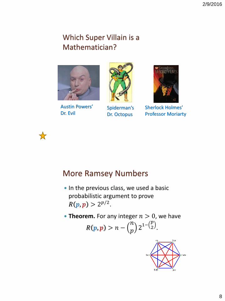
Which Super Villain is a Mathematician?

Austin Powers’Dr. Evil

Sherlock Holmes’Professor Moriarty

Spiderman’sDr. Octopus

More Ramsey Numbers

In the previous class, we used a basic probabilistic argument to prove

𝑅 𝑝, 𝑝 > 2𝑝/2.

Theorem. For any integer 𝑛 > 0, we have

𝑅 𝑝, 𝑝 > 𝑛 −𝑛𝑝 21−𝑝2 .

2/9/2016

9

Proof

Consider a random red-blue coloring of 𝐾𝑛 = (𝑉, 𝐸). The color of each edge is chosen uniformly and independently.

For every subset 𝑆 ⊂ 𝑉 of size 𝑝, we denote by 𝑋𝑆 the indicator that 𝑆 induces a monochromatic 𝐾𝑝. We set 𝑋 = 𝑆 =𝑝𝑋𝑆 .

𝐸 𝑋𝑆 = Pr 𝑋𝑆 = 1 = 21−𝑝2

By linearity of expectation, we have

𝐸 𝑋 =

𝑆 =𝑝

𝐸 𝑋𝑆 =𝑛𝑝 21−𝑝2 .

Completing the Proof

We proved that the in a random red-bluecoloring of 𝐾𝑛 the expected number of monochromatic copies of 𝐾𝑝 is

𝑚 =𝑛𝑝 21−𝑝2 .

There exist a coloring with at most𝑚monochromatic 𝐾𝑝’s.

By removing a vertex from each of these copies, we obtain a coloring of 𝐾𝑛−𝑚 with no monochromatic 𝐾𝑝.

2/9/2016

10

Recap

How we used the probabilistic method:

◦ Our first applications were simply about making random choices and showing that we obtain some property with non-zero probability.

◦ We moved to more involved proofs, where we use linearity of expectation to talk about the “expected” result.

◦ In the previous proof, we used a two step method – first we randomly choose an object, and then we alter it. This method is called the alternation method.

Transmission Towers

Problem. A company wants to establish transmission towers in its large compound.

◦ Each tower must be on top of a building and each building must be covered by at least one tower.

◦ We are given the pairs of buildings such that a tower on one covers the other.

◦ We wish to minimize the number of towers.

2/9/2016

11

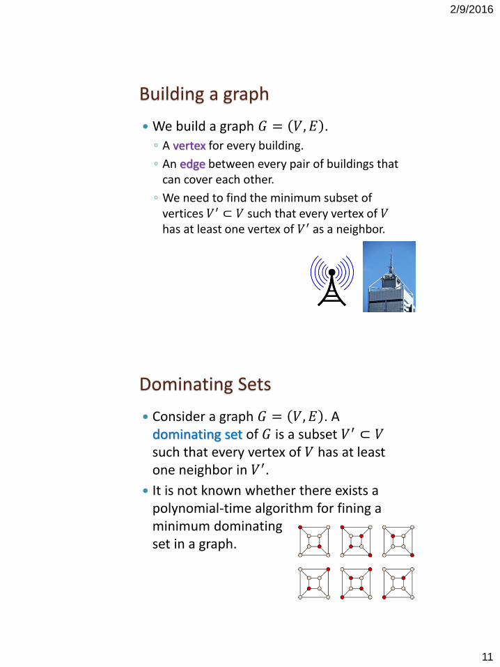
Building a graph

We build a graph 𝐺 = 𝑉, 𝐸 .

◦ A vertex for every building.

◦ An edge between every pair of buildings that can cover each other.

◦ We need to find the minimum subset of vertices 𝑉′ ⊂ 𝑉 such that every vertex of 𝑉has at least one vertex of 𝑉′ as a neighbor.

Dominating Sets

Consider a graph 𝐺 = 𝑉, 𝐸 . A dominating set of 𝐺 is a subset 𝑉′ ⊂ 𝑉such that every vertex of 𝑉 has at least one neighbor in 𝑉′.

It is not known whether there exists a polynomial-time algorithm for fining a minimum dominating set in a graph.

2/9/2016

12

Warm Up

Problem. Let 𝐺 = 𝑉, 𝐸 be a graph with maximum degree 𝑘. Give a lower bound for the size of any dominating set of 𝐺.

Answer.

◦ Every vertex covers itself and at most 𝑚 other vertices, so any dominating set is of size at least

𝑉

𝑘 + 1.

The Case of a Minimum Degree

Theorem. Let 𝐺 = 𝑉, 𝐸 be a graph with minimum degree 𝑘. Then there exists a

dominating set of size at most 𝑛 ⋅1+lg 𝑘

𝑘+1.

Proof. We consider a random subset 𝑆 ⊂ 𝑉 by independently taking each

vertex of 𝑉 with probability 𝑝 =lg 𝑘

𝑘+1.

Let 𝑇 ⊂ 𝑉 ∖ 𝑆 be the vertices that have no neighbors in 𝑆.

◦ 𝑆 ∪ 𝑇 is a dominating set.

2/9/2016

13

𝑆 ⊂ 𝑉 – a random subset formed by independently taking each vertex of 𝑉 with

probability 𝑝 =lg 𝑘+1

𝑘+1.

𝑇 ⊂ 𝑉 ∖ 𝑆 – the vertices with no neighbors in 𝑆.

◦ 𝑆 ∪ 𝑇 is a dominating set.

𝐸 𝑆 = 𝑣∈𝑉 Pr[𝑣 ∈ 𝑆] = 𝑣 𝑝 = 𝑝 𝑉 .

A vertex is in 𝑇 if it is not in 𝑆 and none of its neighbors are in 𝑆. The probability for this is at most 1 − 𝑝 𝑘+1.

𝐸 𝑇 = 𝑣∈𝑉 Pr[𝑣 ∈ 𝑇] ≤ 𝑣 1 − 𝑝𝑘+1

= 1 − 𝑝 𝑘+1 𝑉 .

Proof (cont.)

Completing the Proof

𝑝 =lg 𝑘+1

𝑘+1.

Famous inequality. 1 − 𝑝 ≤ 𝑒−𝑝 for any positive 𝑝.

Thus, 1 − 𝑝 𝑘+1 ≤ 𝑒−𝑝 𝑘+1 =1

𝑘+1.

We proved𝐸 𝑆| + |𝑇 = 𝐸 𝑆 + 𝐸 |𝑇|

≤ 𝑝 + 1 − 𝑝 𝑘+1 𝑉 =lg 𝑘 + 1 + 1

𝑘 + 1|𝑉|.

There must exist a dominating set of size.

2/9/2016

14

How to Choose the Probability?

In the previous problem, we knew to

choose 𝑝 =lg(𝑘+1)

𝑘+1. But how?

◦ When you solve a question and the choice is not uniform, first mark the probability as 𝑝.

◦ At the end of the analysis you will obtain some expression with 𝑝 in it. Choose the value of 𝑝 that optimizes the expression.

The End: Professor Moriarty

Professor Moriarty is a mathematician.

◦ “At the age of twenty-one he wrote a treatise upon the binomial theorem”.

◦ So a combinatorist?!

◦ Dr. Octopus is a nuclear physicist.

◦ Dr. Evil is a medical doctor.