Lecture #8Stability and convergence of hybrid systems

João P. Hespanha

University of Californiaat Santa Barbara

Hybrid Control and Switched Systems

Summary

Lyapunov stability of hybrid systems

Properties of hybrid systems

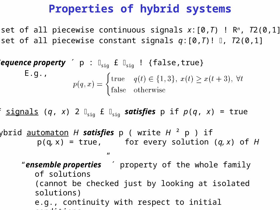
sig ´ set of all piecewise continuous signals x:[0,T) ! Rn, T2(0,1]sig ´ set of all piecewise constant signals q:[0,T)! , T2(0,1]

Sequence property ´ p : sig £ sig ! {false,true}E.g.,

A pair of signals (q, x) 2 sig £ sig satisfies p if p(q, x) = true

A hybrid automaton H satisfies p ( write H ² p ) ifp(q, x) = true, for every solution (q, x) of H

“ensemble properties” ´ property of the whole family of solutions(cannot be checked just by looking at isolated solutions)e.g., continuity with respect to initial conditions…

Lyapunov stability of ODEs (recall)

Definition (continuity definition):A solution x* is (Lyapunov) stable if T is continuous at x*

0 x*(0), i.e.,8 > 0 9 >0 : ||x0 – x*

0|| · ) ||T(x0) – T(x*0)||sig ·

sig ´ set of all piecewise continuous signals taking values in Rn

Given a signal x2sig, ||x||sig › supt¸0 ||x(t)||

ODE can be seen as an operatorT : Rn ! sig

that maps x0 2 Rn into the solution that starts at x(0) = x0

signal norm

supt¸0 ||x(t) – x*(t)|| ·

x(t) x*(t)

pend.m

Lyapunov stability of hybrid systems

mode q1mode q2

1(q1,x–) = q2 ?x2(q1,x–)

sig ´ set of all piecewise continuous signals x:[0,T) ! Rn, T2(0,1]sig ´ set of all piecewise constant signals q:[0,T)! , T2(0,1]

Definition (continuity definition):A solution (q*,x*) is (Lyapunov) stable if T is continuous at (q*(0), x*(0)).

Hybrid automaton can be seen as an operatorT : £ Rn ! sig£ sig

that maps (q0, x0) 2 £ Rn into the solution that starts at q(0) = q0, x(0) = x0

To make sense of continuity we need ways to measure “distances” in £ Rn and sig£ sig

Lyapunov stability of hybrid systems

Definition (continuity definition):A solution (q*,x*) is (Lyapunov) stable if T is continuous at (q0

*, x0*)›(q*(0), x*(0)),

i.e.,

8 > 0 9 >0 : d0( (q*(0), x*(0)) , (q(0), x(0)) ) ·

supt¸ 0 dT( (q*(t), x*(t)) , (q(t), x(t)) ) ·

A few possible “metrics” one cares very much

about the discrete states matching

one does not care at all about the discrete states matching

1. If the solution starts close to (q*,x*) (with respect to the metric d0)it will remain close to it forever(with respect to the metric dT)

2. can be made arbitrarily small by choosing sufficiently small

Note: may actually not be metrics on £ Rn because one may want “zero-distance” between points. However, still define a topology on £ Rn, which is what is really needed to make sense of continuity. See “alternative” lecture #8 for more…

Example #2: Thermostat

73

77

t

turn heater off

turn heater on

q = 2

x

1 1 12 2 2

x · 73 ?

x ¸ 77 ?

q = 1 q = 2

heater

room

x ´ mean temperature

Why?

no trajectory is stable all trajectories are stable

for ddisc “metric” both on initial cond. and trajectory

(d0 = dT = ddisc)

for d0 = ddisc and dT = dcont

some trajectories are stable others unstable

for dcont “metric” both on initial cond. and trajectory

(d0 = dT = dcont)

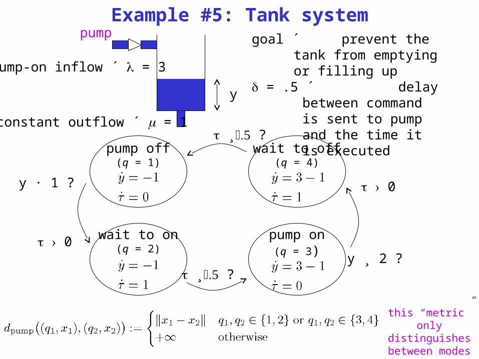
Example #5: Tank system

y

pump goal ´ prevent the tank from emptying or filling up

constant outflow ´ = 1

pump-on inflow ´ = 3

= .5 ´ delay between command is sent to pump and the time it is executed

pump off(q = 1)

wait to on(q = 2)

pump on(q = 3)

wait to off(q = 4)

y · 1 ?

y ¸ 2 ? › 0

¸ ?

¸ ?

› 0

this “metric” only distinguishes between modes based on the state of the pump

Example #4: Inverted pendulum swing-up

u 2 [-1,1] Hybrid controller:

1st pump/remove energy into/from the system by applying maximum force, until E ¼ 0(energy control)

2nd wait until pendulum is close to the upright position

3th next to upright position use feedback linearization controller

pump energy

remove energy

wait stabilize

E 2 [-,] ?

E 2 [-,] ?

E > E < –

+ || ·

Example #4: Inverted pendulum swing-up

u 2 [-1,1]

pump energy

remove energy

wait stabilize

E 2 [-,] ?

E 2 [-,] ?

E > E < –

+ || ·

A possible “metric”

1. for solutions (q*, x*) that start in “s,” we only consider perturbations that also start in “s”2. for solutions (q*, x*) that start outside “s,” the perturbations can start in any state

Asymptotic stability for hybrid systems

Definition:A solution (q*, x*) is (globally) asymptotically stable if it is stable, every solution (q,x) exists globally, and q ! q*, x ! x* as t!1, i.e.,

8 > 0 9 >0 supt¸ dT( (q*(t), x*(t)) , (q(t), x(t)) ) ·

Hybrid automaton can be seen as an operatorT : £ Rn ! sig£ sig

that maps (q0, x0) 2 £ Rn into the solution that starts at q(0) = q0, x(0) = x0

Definition (continuity definition):A solution (q*,x*) is (Lyapunov) stable if T is continuous at (q0

*, x0*)›(q*(0), x*(0)),

i.e.,

8 > 0 9 >0 : d0( (q*(0), x*(0)) , (q(0), x(0)) ) ·

supt¸ 0 dT( (q*(t), x*(t)) , (q(t), x(t)) ) ·

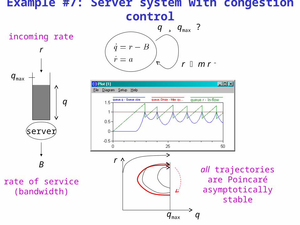
Example #7: Server system with congestion control

r

server

B

rate of service(bandwidth)

incoming rate

q

qmax

q ¸ qmax ?

r m r –

every solution exists globally and converges to a periodic solution that is stable.

Do we have asymptotic stability?

Example #7: Server system with congestion control

r

server

B

rate of service(bandwidth)

incoming rate

q

qmax

every solution exists globally and converges to a periodic solution that is stable.

Do we have asymptotic stability?

q ¸ qmax ?

r m r –

No, its difficult to have asymptotic stability for non-constant solutions due to the “synchronization” requirement.(not even stability… Always?)

Example #2: Thermostat

73

77

t

turn heater off

turn heater on

q = 2

x

1 1 12 2 2

x · 73 ?

x ¸ 77 ?

q = 1 q = 2

heater

room

x ´ mean temperature

no trajectory is stableall trajectories are stable but not asymptotically

for ddisc “metric” both on initial cond. and trajectory

(d0 = dT = ddisc) Why?

for d0 = ddisc and dT = dcont

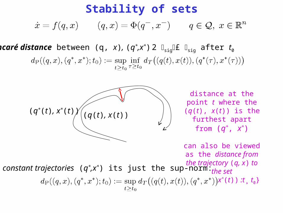
Stability of sets

(q(t), x(t))

For constant trajectories (q*,x*) its just the sup-norm:

distance at the point t where the (q(t), x(t)) is the furthest apart from (q*, x*)

can also be viewed as the distance from the trajectory

(q, x) to the set{(q*(t), x*(t)) :t¸ t0}

(q*(t), x*(t))

Poincaré distance between (q, x), (q*,x*) 2 sig£ sig after t0

Stability of sets

Definition: A solution (q*, x*) is Poincaré asymptotically stable if it is Poincaré stable, every solution (q, x) exists globally, and dP((q,x), (q*,x*); t )!0 as t!1

in more modern terminology one would say that the following set is asymptotically stable: { (q*(t), x*(t)) : t ¸ 0 } ½ £

Definition: A solution (q*, x*) is Poincaré stable if

8 > 0 9 >0 : d0((q(0), x(0)), (q*(0), x*(0))) ·

dP((q*,x*), (q,x); 0) = supt¸ 0 inf¸ 0 dT ((q(t), x(t)), (q*(), x*())) ·

in more modern terminology one would say that the following set is stable{ (q*(t), x*(t)) : t ¸ 0 } ½ £

Poincaré distance between (q, x), (q*,x*) 2 sig£ sig after t0

Example #7: Server system with congestion control

r

server

B

rate of service(bandwidth)

incoming rate

q

qmax

q ¸ qmax ?

r m r –

qmax

r

q

all trajectories are Poincaré

asymptotically stable

To think about …

1. With hybrid systems there are many possible notions of stability.(especially due to the topology imposed on the discrete state)WHICH ONE IS THE BEST?

(engineering question, not a mathematical one)

What type of perturbations do you want to consider on the initial conditions?(this will define the topology on the initial conditions)

What type of changes are you willing to accept in the solution?(this will define the topology on the solution)

2. Even with ODEs there are several alternatives: e.g.,8 > 0 9 >0 : ||x0 – xeq|| · ) supt¸ 0||x(t) – xeq|| ·

or8 > 0 9 >0 : ||x0 – xeq|| · ) s

1 ||x(t) – xeq|| dt · or

8 > 0 9 >0 : ||x0 – x0*|| · ) dP( x, x*; 0 ) ·

(even for linear systems these definitions may differ: Why?)

Lyapunov

integral

Poincaré

Next lecture…

Analysis tools for hybrid systems: Impact maps• Fixed-point theorem• Stability of periodic solutions