linear regression and overfittingspeech.ee.ntu.edu.tw/~tlkagk/courses/ml_2017/lecture/...model...
TRANSCRIPT

RegressionHung-yi Lee
李宏毅
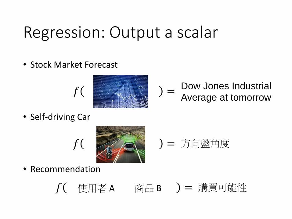
Regression: Output a scalar
• Stock Market Forecast
• Self-driving Car
• Recommendation
𝑓 = Dow Jones Industrial Average at tomorrow
𝑓 =
𝑓 =
方向盤角度
使用者 A 商品 B 購買可能性
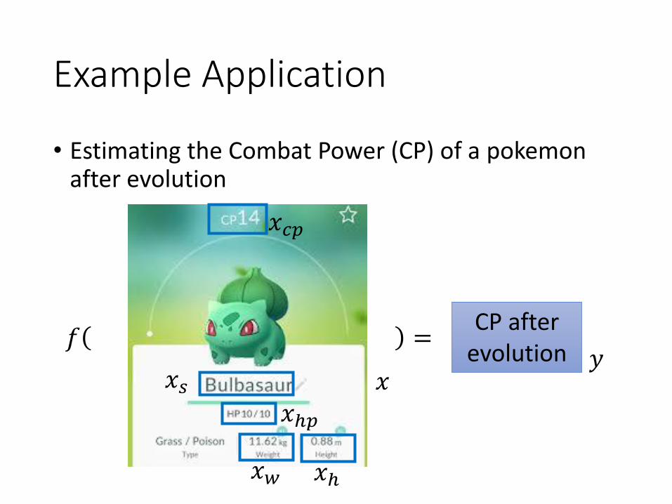
Example Application
• Estimating the Combat Power (CP) of a pokemonafter evolution
𝑓 =CP after
evolution𝑥
𝑦
𝑥𝑐𝑝
𝑥ℎ𝑝
𝑥𝑤 𝑥ℎ
𝑥𝑠
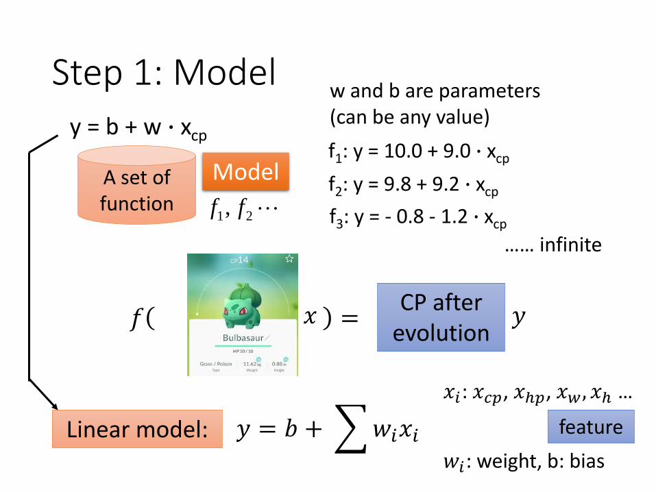
Step 1: Model
A set of function 21, ff
Model
𝑓 =CP after
evolution
Linear model:
f1: y = 10.0 + 9.0 ∙ xcp
f2: y = 9.8 + 9.2 ∙ xcp
f3: y = - 0.8 - 1.2 ∙ xcp
…… infinite
𝑦 = 𝑏 + 𝑤𝑖𝑥𝑖
𝑥𝑖: 𝑥𝑐𝑝, 𝑥ℎ𝑝, 𝑥𝑤 , 𝑥ℎ …
w and b are parameters (can be any value)
𝑥 𝑦
𝑤𝑖: weight, b: bias
y = b + w ∙ xcp
feature
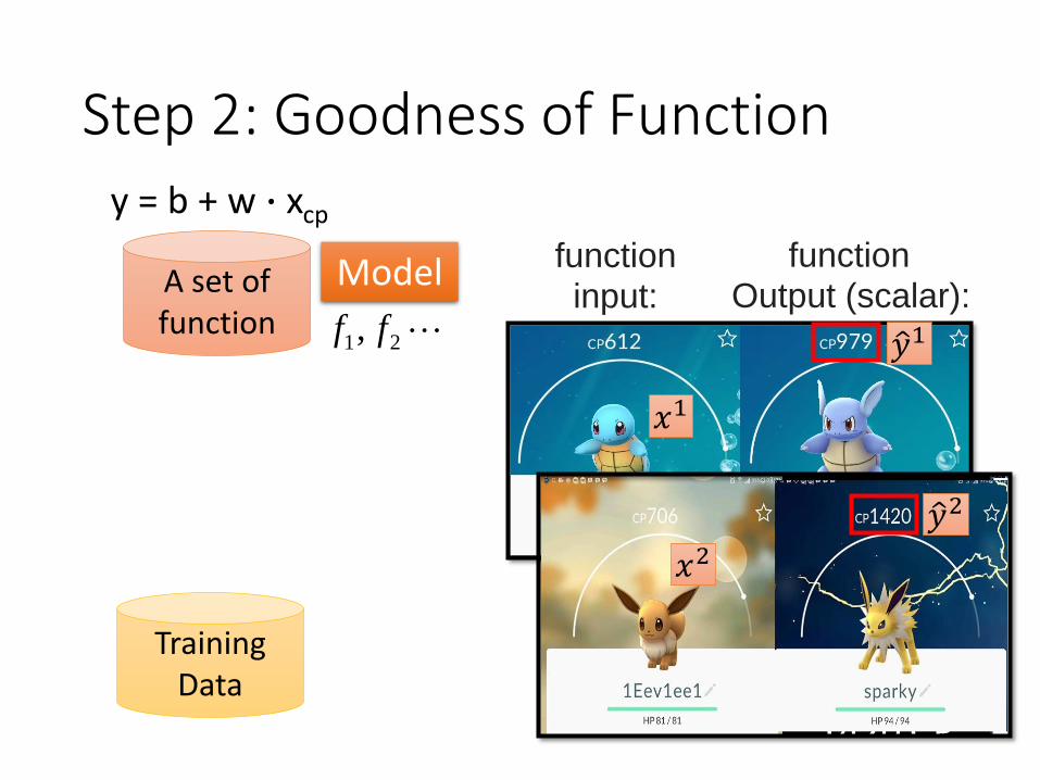
Step 2: Goodness of Function
A set of function 21, ff
Model
TrainingData
function input:
function Output (scalar):
ො𝑦1
𝑥1
𝑥2ො𝑦2
y = b + w ∙ xcp
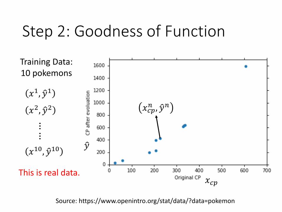
Step 2: Goodness of Function
Source: https://www.openintro.org/stat/data/?data=pokemon
Training Data: 10 pokemons
𝑥𝑐𝑝𝑛 , ො𝑦𝑛
𝑥1, ො𝑦1
𝑥2, ො𝑦2
𝑥10, ො𝑦10
……
𝑥𝑐𝑝
ො𝑦
This is real data.
=
𝑛=1
10
ො𝑦𝑛 − 𝑓 𝑥𝑐𝑝𝑛
2
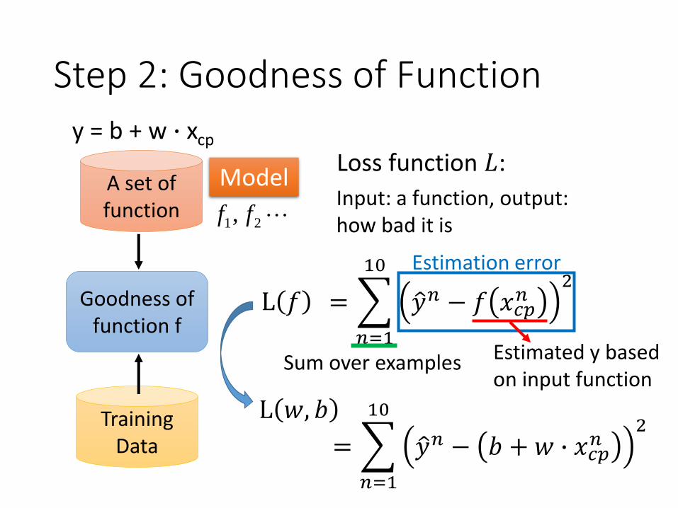
Step 2: Goodness of Function
A set of function 21, ff
Model
TrainingData
Goodness of function f
Loss function 𝐿:
L 𝑓
=
𝑛=1
10
ො𝑦𝑛 − 𝑏 + 𝑤 ∙ 𝑥𝑐𝑝𝑛
2
Input: a function, output: how bad it is
y = b + w ∙ xcp
Estimated y based on input function
Estimation error
Sum over examples
L 𝑤, 𝑏
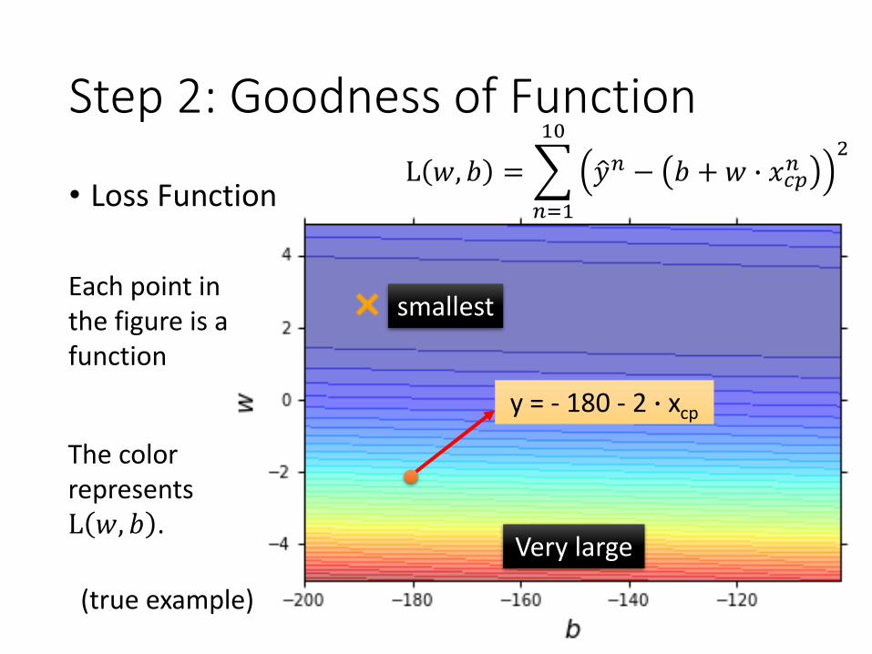
Step 2: Goodness of Function
• Loss Function
Each point in the figure is a function
The color represents L 𝑤, 𝑏 .
(true example)
smallest
Very large
L 𝑤, 𝑏 =
𝑛=1
10
ො𝑦𝑛 − 𝑏 + 𝑤 ∙ 𝑥𝑐𝑝𝑛
2
y = - 180 - 2 ∙ xcp

Step 3: Best Function
A set of function 21, ff
Model
TrainingData
Goodness of function f
Pick the “Best” Function
𝑓∗ = 𝑎𝑟𝑔min𝑓
𝐿 𝑓
𝑤∗, 𝑏∗ = 𝑎𝑟𝑔min𝑤,𝑏
𝐿 𝑤, 𝑏
= 𝑎𝑟𝑔min𝑤,𝑏
𝑛=1
10
ො𝑦𝑛 − 𝑏 + 𝑤 ∙ 𝑥𝑐𝑝𝑛
2
Gradient Descent
L 𝑤, 𝑏
=
𝑛=1
10
ො𝑦𝑛 − 𝑏 + 𝑤 ∙ 𝑥𝑐𝑝𝑛
2

Step 3: Gradient Descent
• Consider loss function 𝐿(𝑤) with one parameter w:
Loss 𝐿 𝑤
w
𝑤∗ = 𝑎𝑟𝑔min𝑤
𝐿 𝑤
(Randomly) Pick an initial value w0
Compute 𝑑𝐿
𝑑𝑤|𝑤=𝑤0
w0
Positive
Negative
Decrease w
Increase w
http://chico386.pixnet.net/album/photo/171572850
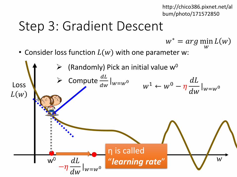
Step 3: Gradient Descent
• Consider loss function 𝐿(𝑤) with one parameter w:
Loss 𝐿 𝑤
w
(Randomly) Pick an initial value w0
Compute 𝑑𝐿
𝑑𝑤|𝑤=𝑤0
w0
http://chico386.pixnet.net/album/photo/171572850
−𝜂𝑑𝐿
𝑑𝑤|𝑤=𝑤0
𝑤1 ← 𝑤0 − 𝜂𝑑𝐿
𝑑𝑤|𝑤=𝑤0
η is called “learning rate”
𝑤∗ = 𝑎𝑟𝑔min𝑤
𝐿 𝑤

Step 3: Gradient Descent
• Consider loss function 𝐿(𝑤) with one parameter w:
Loss 𝐿 𝑤
w
(Randomly) Pick an initial value w0
Compute 𝑑𝐿
𝑑𝑤|𝑤=𝑤0
w0
𝑤1 ← 𝑤0 − 𝜂𝑑𝐿
𝑑𝑤|𝑤=𝑤0
Compute 𝑑𝐿
𝑑𝑤|𝑤=𝑤1
𝑤2 ← 𝑤1 − 𝜂𝑑𝐿
𝑑𝑤|𝑤=𝑤1
…… Many iteration
Local minima
global minima
w1 w2 wT
𝑤∗ = 𝑎𝑟𝑔min𝑤
𝐿 𝑤

Step 3: Gradient Descent
• How about two parameters? 𝑤∗, 𝑏∗ = 𝑎𝑟𝑔min𝑤,𝑏
𝐿 𝑤, 𝑏
(Randomly) Pick an initial value w0, b0
Compute 𝜕𝐿
𝜕𝑤|𝑤=𝑤0,𝑏=𝑏0 ,
𝜕𝐿
𝜕𝑏|𝑤=𝑤0,𝑏=𝑏0
𝑤1 ← 𝑤0 − 𝜂𝜕𝐿
𝜕𝑤|𝑤=𝑤0,𝑏=𝑏0
Compute 𝜕𝐿
𝜕𝑤|𝑤=𝑤1,𝑏=𝑏1 ,
𝜕𝐿
𝜕𝑏|𝑤=𝑤1,𝑏=𝑏1
𝑏1 ← 𝑏0 − 𝜂𝜕𝐿
𝜕𝑏|𝑤=𝑤0,𝑏=𝑏0
𝜕𝐿
𝜕𝑤𝜕𝐿
𝜕𝑏
𝛻𝐿 =
gradient
𝑤2 ← 𝑤1 − 𝜂𝜕𝐿
𝜕𝑤|𝑤=𝑤1,𝑏=𝑏1 𝑏2 ← 𝑏1 − 𝜂
𝜕𝐿
𝜕𝑏|𝑤=𝑤1,𝑏=𝑏1
𝑏
𝑤
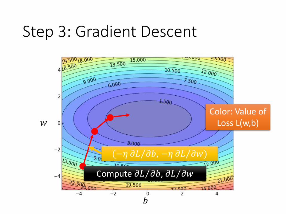
Step 3: Gradient Descent
Compute Τ𝜕𝐿 𝜕𝑏, Τ𝜕𝐿 𝜕𝑤
(−𝜂 Τ𝜕𝐿 𝜕𝑏, −𝜂 Τ𝜕𝐿 𝜕𝑤)
Color: Value of Loss L(w,b)

Step 3: Gradient Descent
• When solving:
• Each time we update the parameters, we obtain 𝜃that makes 𝐿 𝜃 smaller.
𝜃∗ = argmax𝜃
𝐿 𝜃 by gradient descent
𝐿 𝜃0 > 𝐿 𝜃1 > 𝐿 𝜃2 > ⋯
Is this statement correct?
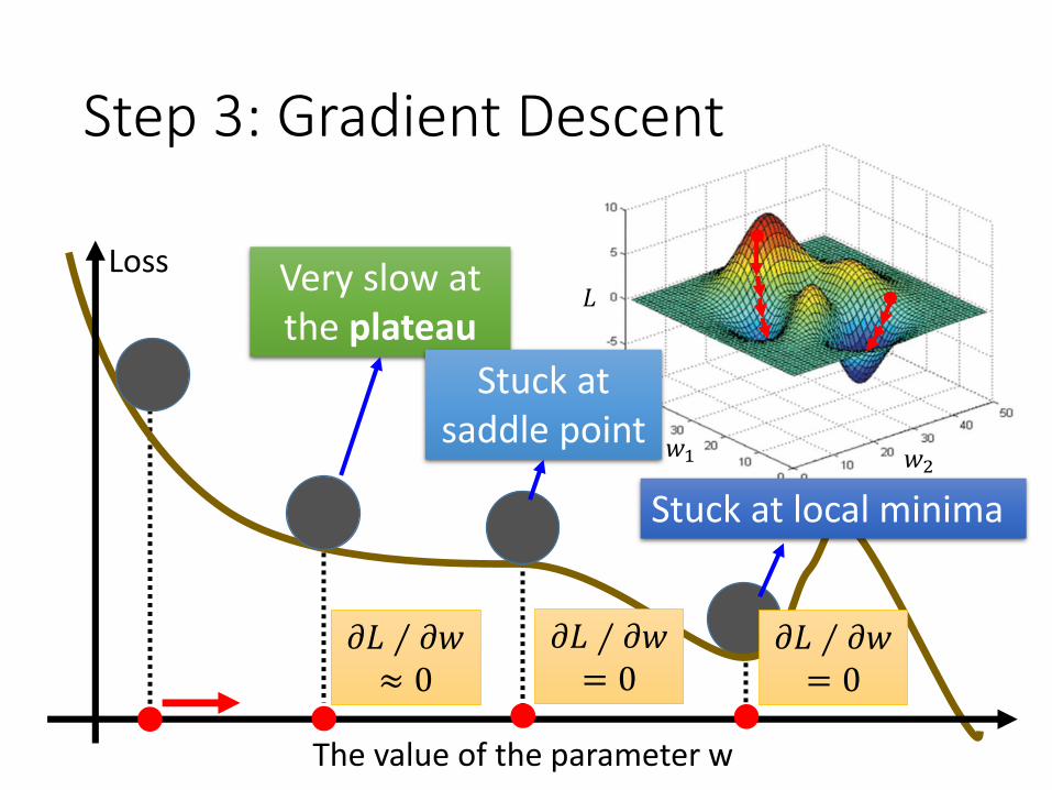
Step 3: Gradient Descent
𝐿
𝑤1 𝑤2
Loss
The value of the parameter w
Very slow at the plateau
Stuck at local minima
𝜕𝐿 ∕ 𝜕𝑤= 0
Stuck at saddle point
𝜕𝐿 ∕ 𝜕𝑤= 0
𝜕𝐿 ∕ 𝜕𝑤≈ 0

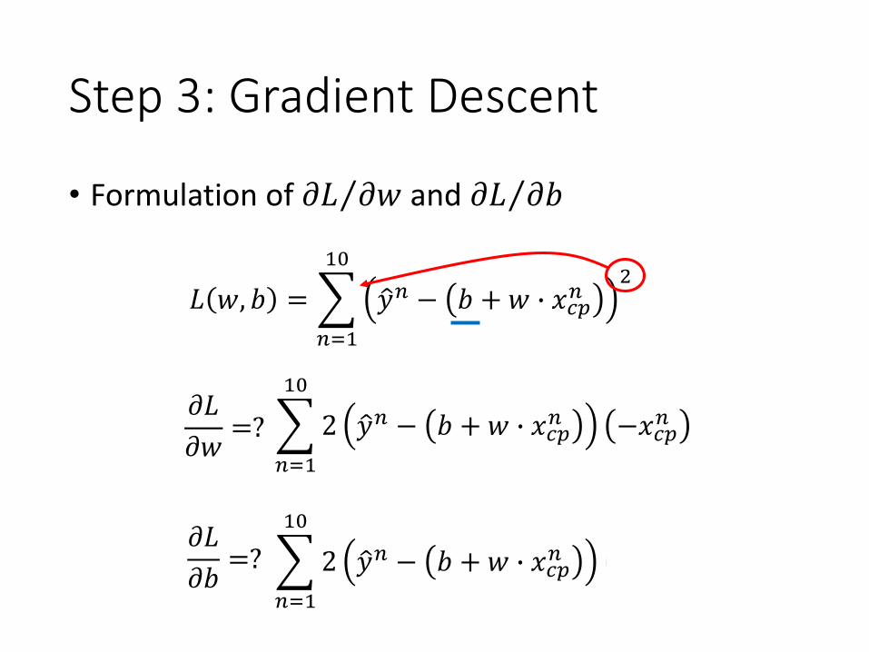
Step 3: Gradient Descent
• Formulation of Τ𝜕𝐿 𝜕𝑤 and Τ𝜕𝐿 𝜕𝑏
𝐿 𝑤, 𝑏 =
𝑛=1
10
ො𝑦𝑛 − 𝑏 + 𝑤 ∙ 𝑥𝑐𝑝𝑛
2
𝜕𝐿
𝜕𝑤=?
𝜕𝐿
𝜕𝑏=?
𝑛=1
10
2 ො𝑦𝑛 − 𝑏 + 𝑤 ∙ 𝑥𝑐𝑝𝑛 −𝑥𝑐𝑝
𝑛
Step 3: Gradient Descent
• Formulation of Τ𝜕𝐿 𝜕𝑤 and Τ𝜕𝐿 𝜕𝑏
𝐿 𝑤, 𝑏 =
𝑛=1
10
ො𝑦𝑛 − 𝑏 + 𝑤 ∙ 𝑥𝑐𝑝𝑛
2
𝜕𝐿
𝜕𝑤=?
𝜕𝐿
𝜕𝑏=?
𝑛=1
10
2 ො𝑦𝑛 − 𝑏 + 𝑤 ∙ 𝑥𝑐𝑝𝑛 −𝑥𝑐𝑝
𝑛
𝑛=1
10
2 ො𝑦𝑛 − 𝑏 + 𝑤 ∙ 𝑥𝑐𝑝𝑛 −1

Step 3: Gradient Descent

How’s the results?
y = b + w ∙ xcp
b = -188.4
w = 2.7
Average Error on Training Data
Training Data
𝑒1
𝑒2
= 31.9 =1
10
𝑛=1
10
𝑒𝑛

How’s the results? - Generalization
y = b + w ∙ xcp
b = -188.4
w = 2.7
Average Error on Testing Data
= 35.0 =1
10
𝑛=1
10
𝑒𝑛
What we really care about is the error on new data (testing data)
Another 10 pokemons as testing data
How can we do better?
> Average Error on Training Data (31.9)
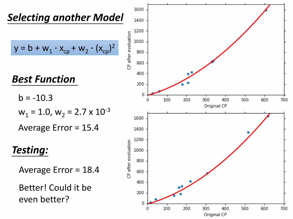
Selecting another Model
Testing:
Average Error = 18.4
y = b + w1 ∙ xcp + w2 ∙ (xcp)2
Average Error = 15.4
Best Function
b = -10.3
w1 = 1.0, w2 = 2.7 x 10⁻³
Better! Could it be even better?

Selecting another Model
Testing:
Average Error = 18.1
Average Error = 15.3
Best Function
b = 6.4, w1 = 0.66
w2 = 4.3 x 10⁻³
w3 = -1.8 x 10⁻⁶
Slightly better. How about more complex model?
y = b + w1 ∙ xcp + w2 ∙ (xcp)2
+ w3 ∙ (xcp)3
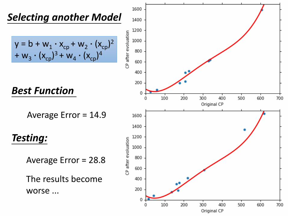
Selecting another Model
Testing:
Average Error = 28.8
Average Error = 14.9
Best Function
The results become worse ...
y = b + w1 ∙ xcp + w2 ∙ (xcp)2
+ w3 ∙ (xcp)3 + w4 ∙ (xcp)4

Selecting another Model
Testing:
Average Error = 232.1
Average Error = 12.8
Best Function
The results are so bad.
y = b + w1 ∙ xcp + w2 ∙ (xcp)2
+ w3 ∙ (xcp)3 + w4 ∙ (xcp)4
+ w5 ∙ (xcp)5
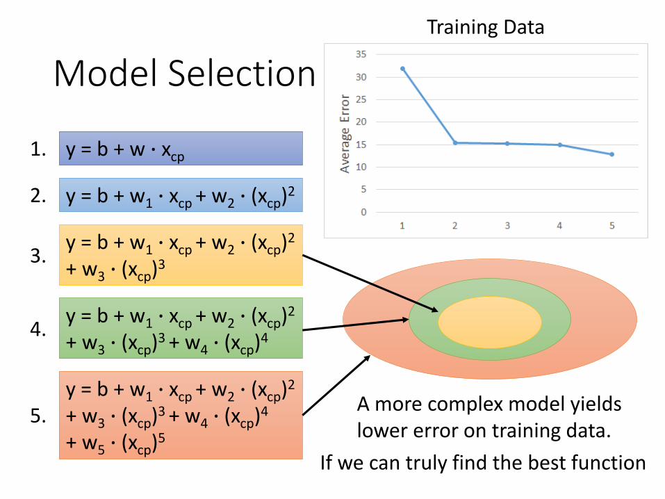
Model Selection
y = b + w1 ∙ xcp + w2 ∙ (xcp)2
y = b + w1 ∙ xcp + w2 ∙ (xcp)2
+ w3 ∙ (xcp)3
y = b + w1 ∙ xcp + w2 ∙ (xcp)2
+ w3 ∙ (xcp)3 + w4 ∙ (xcp)4
y = b + w ∙ xcp
y = b + w1 ∙ xcp + w2 ∙ (xcp)2
+ w3 ∙ (xcp)3 + w4 ∙ (xcp)4
+ w5 ∙ (xcp)5
1.
2.
3.
4.
5.
Training Data
A more complex model yields lower error on training data.
If we can truly find the best function
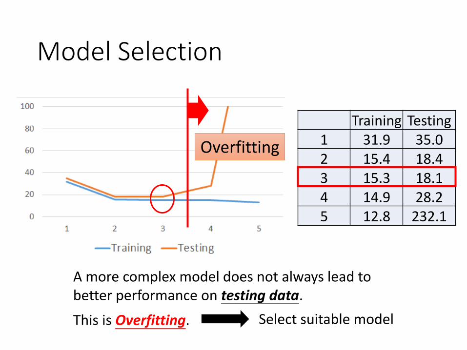
Model Selection
Training Testing1 31.9 35.02 15.4 18.43 15.3 18.14 14.9 28.25 12.8 232.1
A more complex model does not always lead to better performance on testing data.
This is Overfitting.
Overfitting
Select suitable model

Let’s collect more data
There is some hidden factors not considered in the previous model ……

What are the hidden factors?
Eevee
Pidgey
Weedle
Caterpie

Back to step 1: Redesign the Model
x
y
If 𝑥𝑠 = Pidgey:
If 𝑥𝑠 = Weedle:
If 𝑥𝑠 = Caterpie:
If 𝑥𝑠 = Eevee:
𝑦 = 𝑏1 +𝑤1 ∙ 𝑥𝑐𝑝
𝑦 = 𝑏2 +𝑤2 ∙ 𝑥𝑐𝑝
𝑦 = 𝑏3 + 𝑤3 ∙ 𝑥𝑐𝑝
𝑦 = 𝑏4 +𝑤4 ∙ 𝑥𝑐𝑝
Linear model?
𝑦 = 𝑏 + 𝑤𝑖𝑥𝑖
𝑥𝑠 = species of x

Back to step 1: Redesign the Model
𝑦 = 𝑏1 ∙ 𝛿 𝑥𝑠 = Pidgey
+𝑏2 ∙ 𝛿 𝑥𝑠 = Weedle
+𝑏3 ∙ 𝛿 𝑥𝑠 = Caterpie
+𝑏4 ∙ 𝛿 𝑥𝑠 = Eevee
+𝑤1 ∙ 𝛿 𝑥𝑠 = Pidgey 𝑥𝑐𝑝
+𝑤2 ∙ 𝛿 𝑥𝑠 = Weedle 𝑥𝑐𝑝
+𝑤3 ∙ 𝛿 𝑥𝑠 = Caterpie 𝑥𝑐𝑝
+𝑤4 ∙ 𝛿 𝑥𝑠 = Eevee 𝑥𝑐𝑝
𝛿 𝑥𝑠 = Pidgey
=1
=0
Linear model?
𝑦 = 𝑏 + 𝑤𝑖𝑥𝑖
If 𝑥𝑠 = Pidgey
otherwise
If 𝑥𝑠 = Pidgey
𝑦 = 𝑏1 +𝑤1 ∙ 𝑥𝑐𝑝
1
1
0
0
0
0
0
0
𝑥𝑐𝑝
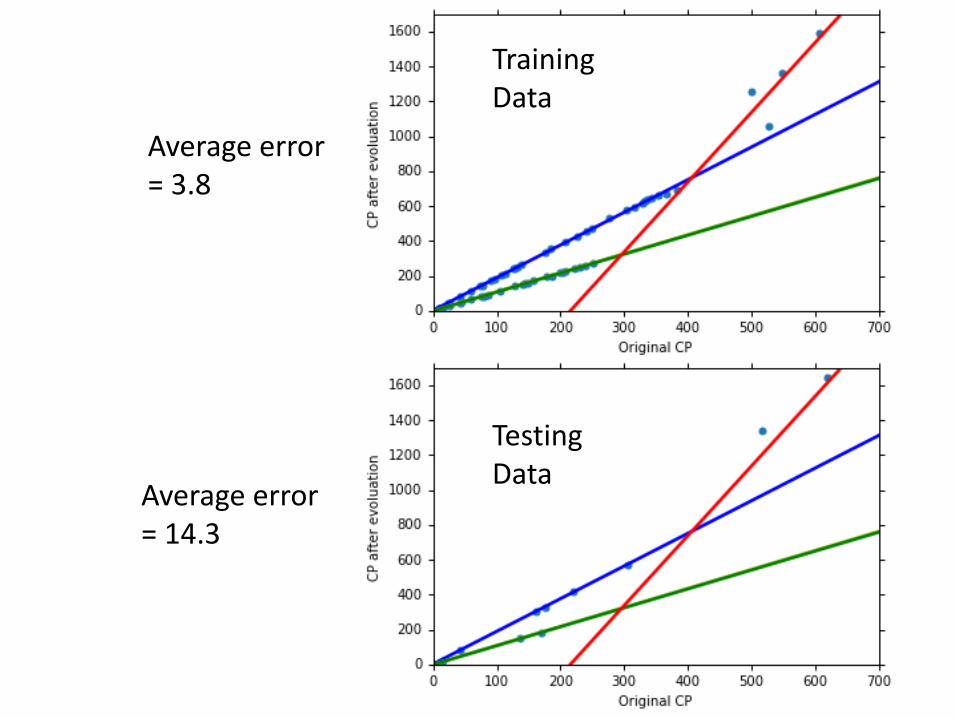
Average error = 14.3
Average error = 3.8
Training Data
TestingData

Are there any other hidden factors?
CP
aft
er e
volu
tio
nC
P a
fter
evo
luti
on
CP
aft
er e
volu
tio
n
weight
HPHeight
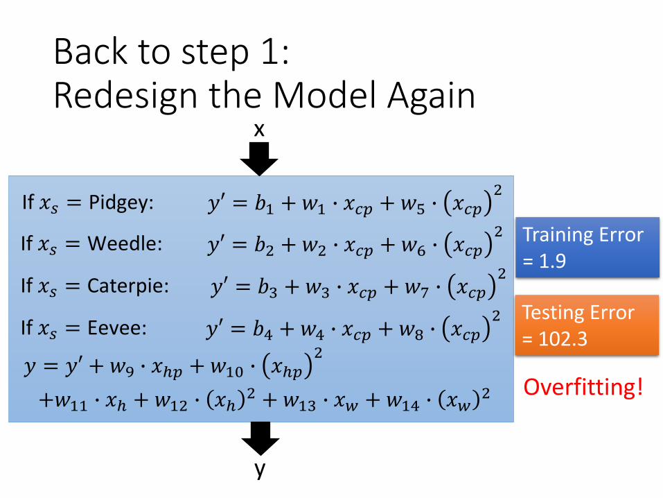
Back to step 1: Redesign the Model Again
y
If 𝑥𝑠 = Pidgey:
If 𝑥𝑠 = Weedle:
If 𝑥𝑠 = Caterpie:
If 𝑥𝑠 = Eevee:
𝑦′ = 𝑏1 +𝑤1 ∙ 𝑥𝑐𝑝 +𝑤5 ∙ 𝑥𝑐𝑝2
𝑦′ = 𝑏2 + 𝑤2 ∙ 𝑥𝑐𝑝 + 𝑤6 ∙ 𝑥𝑐𝑝2
𝑦′ = 𝑏3 +𝑤3 ∙ 𝑥𝑐𝑝 +𝑤7 ∙ 𝑥𝑐𝑝2
𝑦′ = 𝑏4 + 𝑤4 ∙ 𝑥𝑐𝑝 + 𝑤8 ∙ 𝑥𝑐𝑝2
x
𝑦 = 𝑦′ + 𝑤9 ∙ 𝑥ℎ𝑝 +𝑤10 ∙ 𝑥ℎ𝑝2
+𝑤11 ∙ 𝑥ℎ + 𝑤12 ∙ 𝑥ℎ2 +𝑤13 ∙ 𝑥𝑤 + 𝑤14 ∙ 𝑥𝑤
2
Training Error = 1.9
Testing Error = 102.3
Overfitting!
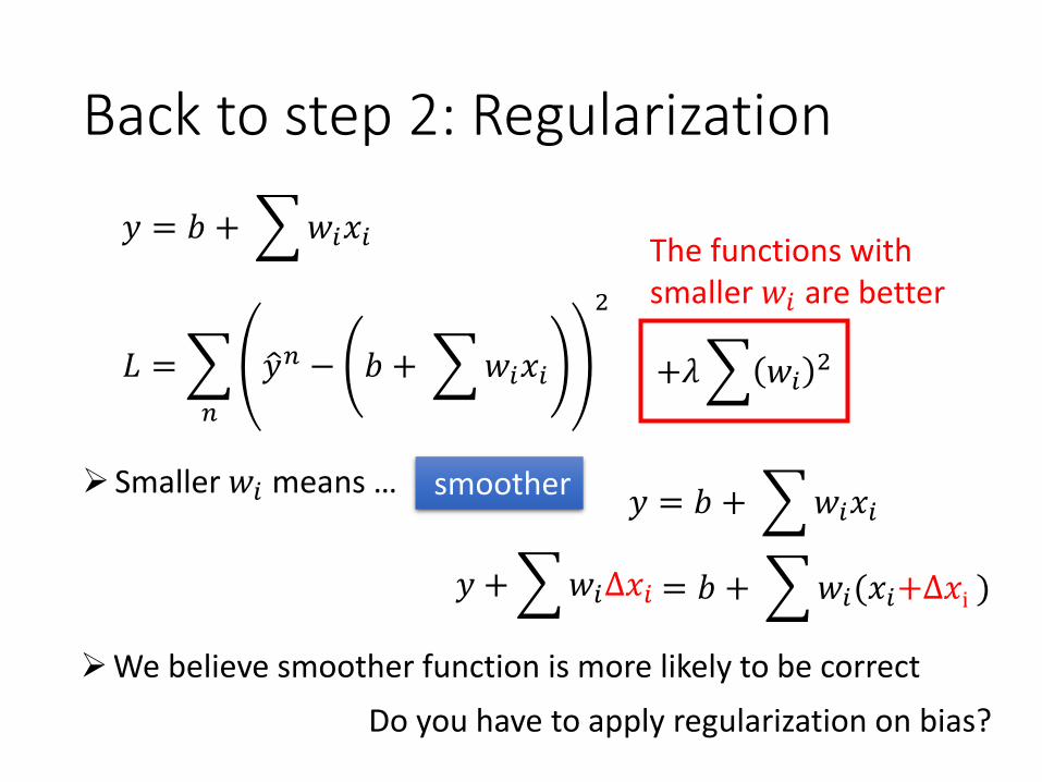
Back to step 2: Regularization
𝐿 =
𝑛
ො𝑦𝑛 − 𝑏 + 𝑤𝑖𝑥𝑖
2
𝑦 = 𝑏 + 𝑤𝑖𝑥𝑖
+𝜆 𝑤𝑖2
The functions with smaller 𝑤𝑖 are better
Smaller 𝑤𝑖 means …𝑦 = 𝑏 + 𝑤𝑖𝑥𝑖
We believe smoother function is more likely to be correct
Do you have to apply regularization on bias?
= 𝑏 + 𝑤𝑖(𝑥𝑖+Δ𝑥i )𝑦 +𝑤𝑖Δ𝑥𝑖
smoother

Regularization𝜆 Training Testing
0 1.9 102.31 2.3 68.7
10 3.5 25.7100 4.1 11.1
1000 5.6 12.810000 6.3 18.7
100000 8.5 26.8
Training error: larger𝜆, considering the training error less
We prefer smooth function, but don’t be too smooth.
smoother
Select 𝜆 obtaining the best model
How smooth?
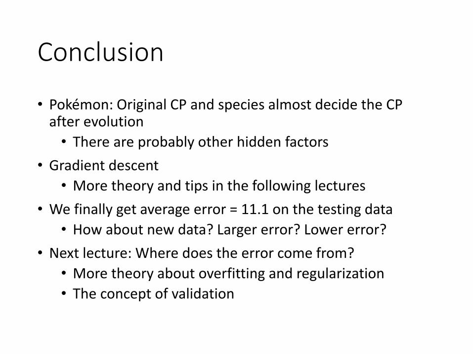
Conclusion
• Pokémon: Original CP and species almost decide the CP after evolution
• There are probably other hidden factors
• Gradient descent
• More theory and tips in the following lectures
• We finally get average error = 11.1 on the testing data
• How about new data? Larger error? Lower error?
• Next lecture: Where does the error come from?
• More theory about overfitting and regularization
• The concept of validation

Reference
• Bishop: Chapter 1.1
Acknowledgment
• 感謝鄭凱文同學發現投影片上的符號錯誤
• 感謝童寬同學發現投影片上的符號錯誤
• 感謝黃振綸同學發現課程網頁上影片連結錯誤的符號錯誤