Policy Research Working Paper 9629

Machine Learning in International Trade Research

Evaluating the Impact of Trade Agreements

Holger BreinlichValentina Corradi

Nadia RochaMichele Ruta

J.M.C. Santos SilvaTom Zylkin

Development Economics Development Research Group &Macroeconomics, Trade and Investment Global PracticeApril 2021

Pub

lic D

iscl

osur

e A

utho

rized

Pub

lic D

iscl

osur

e A

utho

rized

Pub

lic D

iscl

osur

e A

utho

rized

Pub

lic D

iscl

osur

e A

utho

rized

Produced by the Research Support Team

Abstract

The Policy Research Working Paper Series disseminates the findings of work in progress to encourage the exchange of ideas about development issues. An objective of the series is to get the findings out quickly, even if the presentations are less than fully polished. The papers carry the names of the authors and should be cited accordingly. The findings, interpretations, and conclusions expressed in this paper are entirely those of the authors. They do not necessarily represent the views of the International Bank for Reconstruction and Development/World Bank and its affiliated organizations, or those of the Executive Directors of the World Bank or the governments they represent.

Policy Research Working Paper 9629

Modern trade agreements contain a large number of pro-visions in addition to tariff reductions, in areas as diverse as services trade, competition policy, trade-related invest-ment measures, or public procurement. Existing research has struggled with overfitting and severe multicollinearity problems when trying to estimate the effects of these pro-visions on trade flows. Building on recent developments in the machine learning and variable selection literature, this

paper proposes data-driven methods for selecting the most important provisions and quantifying their impact on trade flows, without the need of making ad hoc assumptions on how to aggregate individual provisions. The analysis finds that provisions related to antidumping, competition policy, technical barriers to trade, and trade facilitation are asso-ciated with enhancing the trade-increasing effect of trade agreements.

This paper is a product of the Development Research Group, Development Economics and the Macroeconomics, Trade and Investment Global Practice. It is part of a larger effort by the World Bank to provide open access to its research and make a contribution to development policy discussions around the world. Policy Research Working Papers are also posted on the Web at http://www.worldbank.org/prwp. The authors may be contacted at h.breinlich@surrey.ac.uk, v.corradi@surrey.ac.uk, nrocha@worldbank.org, mruta@worldbank.org, jmcss@surrey.ac.uk, and tzylkin@richmond.edu.

Machine Learning in International Trade Research —Evaluating the Impact of Trade Agreements∗

Holger Breinlich† Valentina Corradi‡ Nadia Rocha§

Michele Ruta¶ J.M.C. Santos Silva‖ Tom Zylkin∗∗

KEY WORDS: Lasso, Machine Learning, Preferential Trade Agreements, Deep TradeAgreements.JEL CLASSIFICATION: F14, F15, F17.

∗Research for this paper has been in part supported by the World Bank’s Multidonor Trust Fundfor Trade and Development. The findings, interpretations, and conclusions expressed in this paper areentirely those of the authors. They do not necessarily represent the views of the International Bank forReconstruction and Development/World Bank and its affi liated organizations, or those of the ExecutiveDirectors of the World Bank or the governments they represent. We also gratefully acknowledge financialsupport through ESRC grant EST013567/1, and thank Scott Baier, Maia Linask, Yoto Yotov, andseminar participants at the World Bank Economics of Deep Trade Agreements Seminar Series for usefulcomments. Alvaro Espitia and Jiayi Ni provided excellent research assistance. The usual disclaimerapplies.†University of Surrey, CEP and CEPR. Email: h.breinlich@surrey.ac.uk‡University of Surrey. Email: v.corradi@surrey.ac.uk§World Bank. Email: nrocha@worldbank.org.¶World Bank. Email: mruta@worldbank.org.‖University of Surrey. Email: jmcss@surrey.ac.uk.∗∗University of Richmond. Email: tzylkin@richmond.edu.

1 Introduction

International trade is of vital importance for modern economies, and governments aroundthe world try to shape their countries’export and import patterns through numerousinterventions. Given the diffi culties facing multilateral trade negotiations through theWorld Trade Organization (WTO), in the last two decades countries have increasinglyturned their focus to preferential trade agreements (PTAs) involving only one or a smallnumber of partners. At the same time, attention has shifted from the reduction of importtariffs to the role of non-tariff barriers and behind-the-border policies, such as differencesin regulations, technical standards or intellectual property rights protection. Accordingly,modern trade agreements contain a host of provisions besides tariff reductions, in areasas diverse as services trade, competition policy, trade-related investment measures, orpublic procurement (Hofmann, Osnago, and Ruta, 2017).Against this background, researchers and policy makers interested in the effects of

trade agreements face diffi cult challenges. In particular, recent research has tried to movebeyond estimating the overall impact of PTAs and to establish the relative importanceof individual trade agreement provisions in determining an agreement’s overall impact(e.g., Kohl, Brakman, and Garretsen, 2016, Mulabdic, Osnago, and Ruta, 2017, Dhingra,Freeman, and Mavroeidi, 2018, and Regmi and Baier, 2020). However, such attemptsface the diffi culty that the large number of provisions, and the fact that similar provisionsappear in different trade agreements, create severe multicollinearity problems, whichmake it very diffi cult to identify the effects of individual provisions. Traditional methodssuch as gravity regressions of trade flows on dummies for individual provisions are notable to deal with such multicollinearity. Instead, researchers have grouped or aggregatedprovisions in different ways. For example, Mattoo, Mulabdic, and Ruta (2017) usethe count of provisions in an agreement as a measure of its ‘depth’, hence implicitlygiving equal weight to each measure. Dhingra, Freeman, and Mavroeidi (2018) overcomemulticollinearity problems by grouping services, investment, and competition provisionsand examining the effect of these “provision bundles”on trade flows.In this paper we propose a new method to estimate the impact of individual provi-

sions on trade flows that does not require ad hoc assumptions to aggregate individualprovisions. Instead, we propose a data-driven method based on recent developmentsin the machine learning and variable selection literature to select the most importantprovisions and quantify their impact on trade flows.In doing so, we build on recent advances in variable selection methods that address

diffi culties arising from a key feature exhibited by trade data, namely the high degree ofcorrelation between individual PTA provisions. We propose an extension of the Belloni,Chernozhukov, Hansen, and Kozbur (2016) approach to the case of nonlinear modelswith high-dimensional fixed effects, which have become standard in the analysis of tradeflows in recent years (see, for example, Head and Mayer, 2014, Yotov, Piermartini, Mon-teiro, and Larch, 2016). In particular, we use a Poisson pseudo-maximum likelihood(PPML) version of the well-known lasso (Least Absolute Shrinkage and Selection Oper-ator) method for variable selection (see, for example, Hastie, Tibshirani, and Friedman,2009) and show how to choose the tuning parameter of this estimator using either a

2

plug-in method based on Belloni, Chernozhukov, Hansen, and Kozbur (2016) or cross-validation. Notably, this requires overcoming a number of practical problems inherentin the nature of trade data, such as the nonlinearity of the underlying gravity model andthe need to control for multilateral resistance and unobserved trade barriers.We apply our method to a comprehensive data set on PTA provisions recently made

available by the World Bank (Mattoo, Rocha and Ruta, 2020). Importantly, this data-base is very rich, to the point where the number of provision variables we consider islarger than the number of PTAs we observe in our data. In addition, due to templateeffects and possible synergies between groups of provisions, these provision variables canbe highly correlated with one another. For these reasons, we complement our plug-inlasso results with a novel methodology that seeks to identify potentially important vari-ables that may have been missed in the initial lasso step. As we show using simulationevidence, this new method, termed the “iceberg lasso”, presents a favorable balancebetween the rigor of the plug-in lasso and the lenience of cross-validation methods insmall-to-moderate samples where the true causal variables may be highly correlatedwith an unknown number of other variables in the data set. To be clear, this two-stepapproach does not completely answer the question of “which provisions matter most fortrade?”but it does lead to substantial improvements in our ability to find the correctprovision variables and narrow down the number of potential candidates in the presenceof such rich data.Our work contributes to several different literatures. Most directly, we contribute to

the large and growing literature on the effects of PTAs on trade flows. This literaturehas been predominantly interested in estimating the overall effects of trade agreementsrather than individual provisions (see, for example, Baier and Bergstrand, 2007). Morerecently, attention has shifted to trying to decompose the overall PTA effect and to dis-entangle the effects of individual trade agreement provisions. As previously discussed,this literature often needs to make strong assumptions about the importance of indi-vidual provisions or needs to aggregate them in essentially arbitrary ways (see Mattoo,Mulabdic, and Ruta, 2017; Dhingra, Freeman, and Mavroeidi, 2018). We propose in-stead a novel set of methods to select the most important provisions and to quantifytheir impact on trade flows. To provide some headline results, our plug-in lasso resultsfind that 6 provisions related to antidumping, competition policy, technical barriers totrade, and trade facilitation are associated with enhancing the trade-increasing effect oftrade agreements. When we then use our iceberg lasso procedure to look beyond the“tip”of the proverbial iceberg, we subsequently identify a set of 43 provisions out of 305provision variables in our data that may be impacting trade. For some comparison, amore conventional approach based on cross-validation selects 124 provisions as being rel-evant and, based on our simulations, is actually less likely to include all of the “correct”provisions.In addition, we contribute to the subset of the machine learning literature inter-

ested in variable selection. In particular, we extend and adapt existing work by Belloni,Chernozhukov, Hansen, and Kozbur (2016) to make it applicable to the context of inter-national trade flows and trade agreements. This requires an extension to the estimationof nonlinear models with high-dimensional fixed effects using PPML. The international

3

trade context also throws up some interesting challenges when trying to select the tuningparameter that governs the extent to which our PPML-lasso estimator penalizes coeffi -cients on included variables and hence selects included variables. In particular, standardcross-validation methods such as k-fold or leave-one-out approaches are not feasible inpractice, requiring us to propose a novel approach based on out-of-sample predictions ofthe effects of PTAs. We find that the number of provisions selected when the tuning pa-rameter is chosen by cross-validation is too large to have a meaningful interpretation andthat, in contrast, the number of provisions identified when using the plug-in penalty istoo small to allow us to be confident that it includes the majority of relevant provisions.The two-step method that we propose builds on the results obtained using the plug-inpenalty and identifies an additional set of provisions that may have a causal effect ontrade.Finally, we contribute to a small existing literature that has used machine learning

and other related methods to study the effects of trade agreements in a gravity context.For example, Regmi and Baier (2020) use an unsupervised learning method to groupPTAs by textual similarity, so as to provide a more nuanced notion of PTA depth.Following from a similar motivation, Hofmann, Osnago, and Ruta (2017) propose anearlier depth measure for PTAs based on principal components analysis applied to theirprovisions data. In contrast, Baier, Yotov, and Zylkin (2019) use a two-step methodologywhere pair-specific PTA effects are estimated in a first stage and then predicted out ofsample using country- and pair-specific variables.The rest of this paper is structured as follows. Section 2 presents the data on PTA

provisions and provides a descriptive analysis of these data, highlighting a number ofstylized facts about the provisions present in recent trade agreements. Section 3 intro-duces the variable selection problem in the three-way gravity model context and explainshow we implement PPML-lasso estimation with high-dimensional fixed effects. It alsoincludes simulation evidence comparing relative performance of different lasso methodsin a simplified setting with high correlation between regressors. Section 4 applies ourmethods to our database on PTA provisions and shows which individual provisions arethe strongest predictors of trade flows. Section 5 concludes.

2 Data

Our analysis combines data on international trade flows from Comtrade with the newdatabase on the content of PTAs that has been collected by Mattoo, Rocha and Ruta(2020). On trade, we use merchandise trade exports between 1964 and 2016 from 220exporters to 270 importers. Country pairs without export information are consideredas zeros. The database on the content of trade agreements includes information on 283PTAs that have been signed and notified to the WTO between 1958 and 2017. The datafocus on the sub-sample of 18 policy areas that are most frequently covered in tradeagreements —defined as areas that are present in 20 percent or more of the agreementsthat have been mapped in Hofmann, Osnago, and Ruta (2017). These policy areas rangefrom environmental laws and labor market regulations, that are covered in roughly 20

4

percent of the PTAs, to areas such as export taxes and trade facilitation that are presentin over 80 percent of the agreements (see Figure 1).

Figure 1: Share of PTAs that cover selected policy areas

Figure shows the share of PTAs that cover a policy area. Source: Mattoo, Rocha and Ruta (2020).

For each agreement and policy area, the database provides granular information onthe specific provisions covering stated objectives and substantive commitments, as wellas aspects relating to transparency, procedures and enforcement. The coding exercisefocuses on the legal text of the agreements and therefore excludes information on theactual implementation of the commitments included in the agreements.1

To alleviate the problems caused by the high dimensionality of the data and the highlevel of correlation across the provisions included in the agreements, the analysis pre-sented in this paper focuses on a sub-set of “essential”provisions. This includes the setof substantive provisions (those that require specific integration/liberalization commit-ments and obligations) plus the disciplines among procedures, transparency, enforcementor objectives, which are viewed as indispensable and complementary to achieving thesubstantive commitments. Non-essential provisions are referred to as “corollary”.2 Theshare of essential provisions in the total number of provisions included in an agreementranges from less than 10 percent for public procurement, movement of capital and visaand asylum, to more than 50 percent for policy areas such as environmental laws andlabor market regulations. Overall, the sub-set of essential provisions represents almostone-third (305/937) of the total number of provisions coded in this exercise (see Table1).

1In this data set, information coming from secondary law (the body of law that derives from theprinciples and objectives of the treaties) has not been coded. This is of particular importance foragreements such as the EU, since most policy areas covered have used secondary law such as regulations,directives, and other legal instruments to pursue integration.

2The classification into essential and corollary in the database is based on experts’knowledge and,hence, is subjective.

5

Table 1: Distribution of essential provisions by policy areaNumber of Number of

Policy Area provisions Essential provisions ShareAnti-dumping and Countervailing Duties 53 11 28.8%Competition Policy 35 14 40.0%Environmental Laws 48 27 56.3%Export Taxes 46 23 50.0%Intellectual Property Rights 120 67 55.8%Investment 57 15 26.3%Labor Market Regulations 18 12 66.7%Movement of Capital 94 8 8.5%Public Procurement 100 5 5.0%Rules of Origin 38 19 50.0%Sanitary and Phytosanitary 59 24 40.7%Services 64 21 32.8%State-Owned Enterprises 53 13 24.5%Subsidies 36 13 36.1%Technical Barriers to Trade 34 19 55.9%Trade Facilitation and Customs 52 11 21.2%Visa and Asylum 30 3 10.0%Total 937 305 32.6%

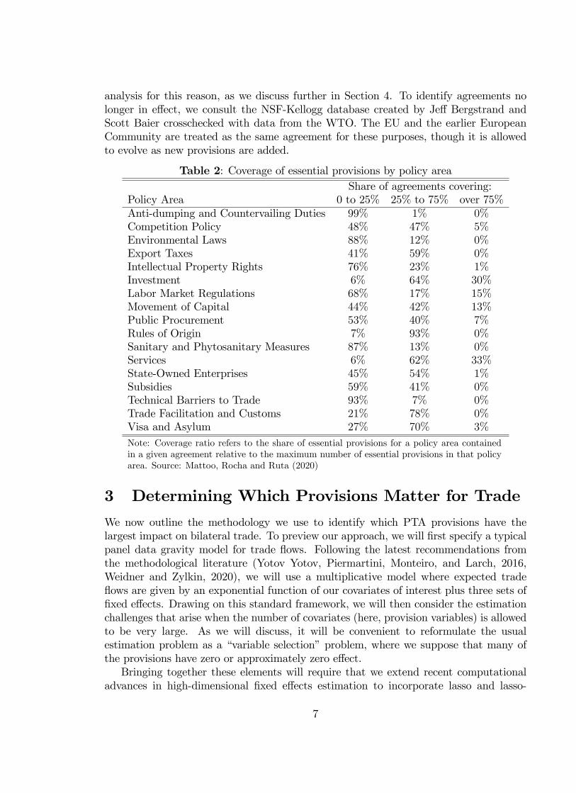
The coverage of essential provisions also varies widely across trade agreements anddisciplines, indicating that not all PTAs cover the same set of essential provisions. Asshown in Table 2, more than 3/4 of agreements cover 25 percent or less of essentialprovisions included in policy areas such as environmental laws, antidumping, sanitaryand phytosanitary measures, and technical barriers to trade. Conversely, for policyareas such as visa and asylum, rules of origin, and trade facilitation and customs, morethan 70 percent of the mapped agreements cover between 25 and 75 percent of essentialprovisions. With the exception of services and investment, coverage of more than 75percent of essential provisions is rare and happens in less than 15 percent of the mappedagreements.One important caveat regarding this data set is that it does not cover all of the

trade agreements that have been in force during the period under study. Specifically,our information on provisions is limited to agreements that are in effect in present day,i.e., excluding any agreements that are no longer in effect. For this reason, we dropobservations associated with an agreement no longer in effect. This means that theeffects of newer agreements are identified by changes in trade relative to when thatpair did not have any agreement rather than relative to pre-existing agreements. Themajority of the observations that are dropped are due to pre-accession agreements thatnew European Union (EU) members sign before joining the EU. Thus, to use one ofthese cases as an example, Italy-Croatia is included in our data for years 1992-2000(after Croatian independence and before the initial EU-Croatia PTA in 2001) and foryear 2016 (after Croatia joins the EU in 2013). The EU is treated differently in our

6

analysis for this reason, as we discuss further in Section 4. To identify agreements nolonger in effect, we consult the NSF-Kellogg database created by Jeff Bergstrand andScott Baier crosschecked with data from the WTO. The EU and the earlier EuropeanCommunity are treated as the same agreement for these purposes, though it is allowedto evolve as new provisions are added.

Table 2: Coverage of essential provisions by policy areaShare of agreements covering:

Policy Area 0 to 25% 25% to 75% over 75%Anti-dumping and Countervailing Duties 99% 1% 0%Competition Policy 48% 47% 5%Environmental Laws 88% 12% 0%Export Taxes 41% 59% 0%Intellectual Property Rights 76% 23% 1%Investment 6% 64% 30%Labor Market Regulations 68% 17% 15%Movement of Capital 44% 42% 13%Public Procurement 53% 40% 7%Rules of Origin 7% 93% 0%Sanitary and Phytosanitary Measures 87% 13% 0%Services 6% 62% 33%State-Owned Enterprises 45% 54% 1%Subsidies 59% 41% 0%Technical Barriers to Trade 93% 7% 0%Trade Facilitation and Customs 21% 78% 0%Visa and Asylum 27% 70% 3%

Note: Coverage ratio refers to the share of essential provisions for a policy area containedin a given agreement relative to the maximum number of essential provisions in that policyarea. Source: Mattoo, Rocha and Ruta (2020)

3 Determining Which Provisions Matter for Trade

We now outline the methodology we use to identify which PTA provisions have thelargest impact on bilateral trade. To preview our approach, we will first specify a typicalpanel data gravity model for trade flows. Following the latest recommendations fromthe methodological literature (Yotov Yotov, Piermartini, Monteiro, and Larch, 2016,Weidner and Zylkin, 2020), we will use a multiplicative model where expected tradeflows are given by an exponential function of our covariates of interest plus three sets offixed effects. Drawing on this standard framework, we will then consider the estimationchallenges that arise when the number of covariates (here, provision variables) is allowedto be very large. As we will discuss, it will be convenient to reformulate the usualestimation problem as a “variable selection”problem, where we suppose that many ofthe provisions have zero or approximately zero effect.Bringing together these elements will require that we extend recent computational

advances in high-dimensional fixed effects estimation to incorporate lasso and lasso-

7

type penalties. It will also require that we introduce our own innovation, the iceberglasso method, which we will motivate as providing a balance between “cross-validation”approaches that tend to select too many variables and more rigorous, “plug-in”methodsthat may select too few. We also include simulation evidence comparing the performanceof these various methods.

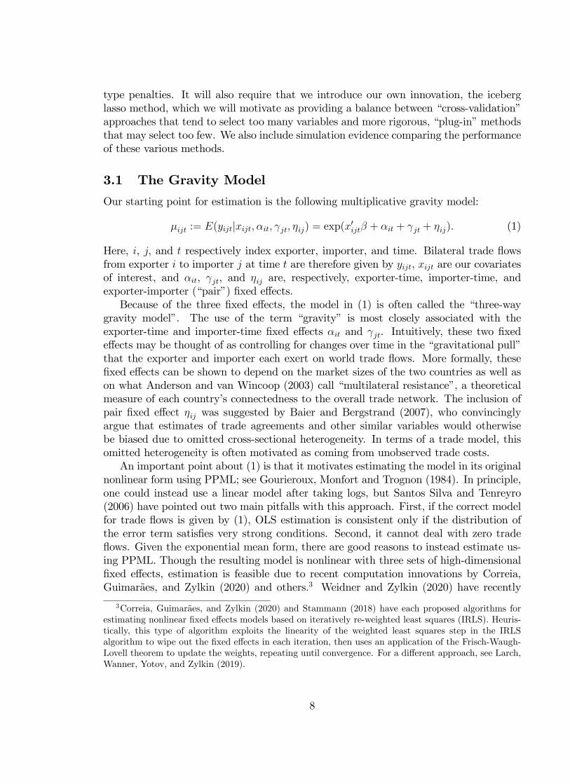
3.1 The Gravity Model

Our starting point for estimation is the following multiplicative gravity model:

µijt := E(yijt|xijt, αit, γjt, ηij) = exp(x′ijtβ + αit + γjt + ηij). (1)

Here, i, j, and t respectively index exporter, importer, and time. Bilateral trade flowsfrom exporter i to importer j at time t are therefore given by yijt, xijt are our covariatesof interest, and αit, γjt, and ηij are, respectively, exporter-time, importer-time, andexporter-importer (“pair”) fixed effects.Because of the three fixed effects, the model in (1) is often called the “three-way

gravity model”. The use of the term “gravity” is most closely associated with theexporter-time and importer-time fixed effects αit and γjt. Intuitively, these two fixedeffects may be thought of as controlling for changes over time in the “gravitational pull”that the exporter and importer each exert on world trade flows. More formally, thesefixed effects can be shown to depend on the market sizes of the two countries as well ason what Anderson and van Wincoop (2003) call “multilateral resistance”, a theoreticalmeasure of each country’s connectedness to the overall trade network. The inclusion ofpair fixed effect ηij was suggested by Baier and Bergstrand (2007), who convincinglyargue that estimates of trade agreements and other similar variables would otherwisebe biased due to omitted cross-sectional heterogeneity. In terms of a trade model, thisomitted heterogeneity is often motivated as coming from unobserved trade costs.An important point about (1) is that it motivates estimating the model in its original

nonlinear form using PPML; see Gourieroux, Monfort and Trognon (1984). In principle,one could instead use a linear model after taking logs, but Santos Silva and Tenreyro(2006) have pointed out two main pitfalls with this approach. First, if the correct modelfor trade flows is given by (1), OLS estimation is consistent only if the distribution ofthe error term satisfies very strong conditions. Second, it cannot deal with zero tradeflows. Given the exponential mean form, there are good reasons to instead estimate us-ing PPML. Though the resulting model is nonlinear with three sets of high-dimensionalfixed effects, estimation is feasible due to recent computation innovations by Correia,Guimarães, and Zylkin (2020) and others.3 Weidner and Zylkin (2020) have recently

3Correia, Guimarães, and Zylkin (2020) and Stammann (2018) have each proposed algorithms forestimating nonlinear fixed effects models based on iteratively re-weighted least squares (IRLS). Heuris-tically, this type of algorithm exploits the linearity of the weighted least squares step in the IRLSalgorithm to wipe out the fixed effects in each iteration, then uses an application of the Frisch-Waugh-Lovell theorem to update the weights, repeating until convergence. For a different approach, see Larch,Wanner, Yotov, and Zylkin (2019).

8

established the consistency and asymptotic distribution of the three-way PPML estima-tor, and Yotov, Piermartini, Monteiro, and Larch (2016) recommend it as the workhorsemethod for estimating the effects of trade policies. It is frequently applied to the contextof trade agreements in particular.Having established these details, our focus is on the set of covariates, xijt. In most

applications in the trade agreements literature, xijt is often either a single variable–i.e., a dummy for the presence of a trade agreement– or minor variants thereof, suchas introducing interactions with either the depth of the agreement or the bilateral char-acteristics of the two countries (Baier, Bergstrand, and Feng, 2014; Baier, Bergstrand,and Clance, 2018). However, a major estimation challenge that arises in our setting isthat we must treat the number of provisions as being very large. With our data set, thishigh dimensionality, combined with the relatively small number of PTAs, leads to im-plausibly large and uninterpretable estimates due to multicollinearity. Furthermore, theestimated model will have poor predictive performance due to overfitting. We thereforemust discuss how the standard gravity estimation approach must be modified in orderto deal with this additional source of high dimensionality.

3.2 Variable Selection and Gravity

The starting point for our methodological innovations is to suppose that only a handfulof our provision variables have a non-negligible effect on trade flows. To be more precise,we have p = 305 essential provision variables, coded as dummies, of which a subset s < pare assumed to have non-zero effects. We do not know s beforehand, nor do we knowthe identities of any of the s provisions that substantively affect trade. Our goal thenis to use statistical methods along with the model described in (1) in order to identifythese provisions.Because of the high dimensionality of xijt, experimenting with different subsets of

provisions to see which has the best performance is unlikely to be fruitful. Instead, weadopt a penalized regression (or “regularization”) approach that involves appending apenalty term to the Poisson pseudo-likelihood one would use to estimate the unpenalizedgravity model. The idea is that the penalty term “shrinks” all estimated coeffi cientstowards zero and forces some of them to be exactly equal to zero. The higher thepenalty, the fewer the variables that are found to have non-zero coeffi cients and aretherefore “selected”. By design, the variables that are selected should be those thatexert the strongest influence on the fit of the model; coeffi cients for variables that arenot as relevant should end up getting shrunken to zero completely.Because of its computational feasibility, the most frequently used approach to this

type of variable selection problem is the lasso, introduced by Tibshirani (1996). In oursetting, the penalized objective function that defines the three-way PPML-lasso is

PL(β, α, γ, η) =1

n

(∑i,j,t

(µijt − yijt lnµijt

))︸ ︷︷ ︸−1×PPML pseudo likelihood

+1

n

p∑k=1

φ̂kλ|βk|︸ ︷︷ ︸Lasso penalty

, (2)

9

where n is the number of observations,4 as in (1) above, µijt = eαit+γjt+ηij+x′ijtβ is the

conditional mean, and λ ≥ 0 and φ̂k ≥ 0 are tuning parameters that determine thepenalty. As indicated in (2), the first term in this expression is the standard PPMLobjective function one would minimize in order to estimate the three-way gravity model.Thus, the PPML-lasso nests PPML as a special case when λ is set to zero.The second term in (2) is a modified lasso penalty that allows for regressor-specific

penalty weights as opposed to having λ as the only tuning parameter as in the standardlasso. Intuitively, larger penalties increasingly shrink the estimated β-coeffi cients towardszero. The coeffi cients for any variables that do not suffi ciently increase the likelihoodare set to exactly zero, thereby giving us a way of identifying which xijt variables toinclude in the final model. For some illustration, if we consider λ→∞, the only way tominimize PL is to set all β̂ks equal to zero, meaning that no variables are selected. As inBelloni, Chernozhukov, Hansen, and Kozbur (2016), we will use the regressor-specific φ̂kpenalty terms to iteratively refine the model while also constructing them appropriatelyto reflect any heteroskedasticity and within-pair correlation featured in the data.Importantly, the fixed effects parameters α, γ, and η are not penalized. This is

mainly because there is no reason to believe that most of the fixed effects parameters areactually zero. In addition, it turns out they do not pose special issues for computation.This is because they do not depend on the penalty. As such, for any given β, the fixedeffects can be obtained by solving their usual PPML first-order conditions from thestandard unpenalized regression approach. In practice, this means that the fixed effectscan actually be dealt with in the exact same manner as in Correia, Guimarães, and Zylkin(2020). More details on our computational methods are provided in the Appendix, but,basically, we use the original HDFE-IRLS algorithm of Correia, Guimarães, and Zylkin(2020) to take care of the fixed effects but replace the weighted linear regression stepfrom that algorithm with a weighted lasso regression.5

3.3 Implementing the Lasso

The next question of course is how to determine the tuning parameters λ and φ̂k. As astarting point, the two existing approaches we will first examine are the “plug-in”lasso ofBelloni, Chernozhukov, Hansen, and Kozbur (2016) and the traditional cross-validationapproach, both of which we have modified to fit the demands of the three-way PPMLsetting. As we will discuss, each of these methods has its strengths and weaknesses.Therefore, we will then turn to describing an extension of the plug-in lasso, termed the“iceberg lasso”, that is intended to address one of the plug-in lasso’s key shortcomingsin this context.

4Naturally, the number of observations will depend on the number of countries for which we havedata and on the number of years we observe them. For simplicity, we do not make that relation explicit.

5For the lasso regression step, we use the coordinate descent algorithm of Friedman, Hastie, andTibshirani (2010).

10

Plug-in Lasso

The plug-in lasso is so-named because it specifies appropriate functional forms for thepenalty parameters based on statistical theory and then uses plug-in estimates for theseparameters. It is therefore a relatively “theory-driven”approach to the variable selectionproblem, whereas cross-validation, discussed next, is a more traditional machine learningmethod that relies on out-of-sample prediction. The plug-in lasso was first proposed byBelloni, Chen, Chernozhukov, and Hansen (2012), though the specific implementation webuild on is the panel data lasso method of Belloni, Chernozhukov, Hansen, and Kozbur(2016), which allows for correlated errors within cross-sectional units.Without delving too much into technical details, which we defer to the Appendix,

variable selection using the plug-in lasso can be thought of as involving the followingthree ingredients:

i. The absolute value of the score for each βk when evaluated at 0,

ii. The standard error of the score for each βk,

iii. Values for λ and φ̂k set high enough so that the absolute value of the score for βkmust be statistically large relative to its standard error in order for regressor xijt,kto be selected.

Intuitively, the value of the score reflects the impact that a small change in βk hason the fit of the model. When evaluated at 0, it tells us how much the fit of themodel improves when we make βk non-zero. The standard logic of the lasso is that thisimprovement in fit must be large relative to the penalty in order for β̂k to be non-zero.One of the main innovations of the plug-in lasso is to allow the regressor-specific penaltyφ̂k to adjust to reflect the standard error of the score. This way, we counteract thepossibility that regressors could be mistakenly selected due to estimation noise ratherthan because of their true impact on the model. These regressor-specific penalties playan important role in the presence of heteroskedasticity, which of course is an importantfeature of trade data. Since the gravity context often assumes that errors are correlatedover time within pair, we take this correlation into account as well in constructing thesepenalty weights.A principal advantage of the plug-in lasso is that it is very rigorous in terms of the

number of variables it selects. As shown by Drukker and Liu (2019), the plug-in methodoffers superior performance versus cross-validation approaches in finite samples, in largepart because these other methods tend to select too many variables. Furthermore, the“post-lasso”estimates obtained using unpenalized PPML on the covariates selected bythe plug-in lasso have a “near-oracle”property that ensures they will capture the correctmodel if the sample is suffi ciently large relatively to the number of potential regressors(see Belloni, Chen, Chernozhukov, and Hansen, 2012).6

6The “oracle”property of estimators such as the adaptive lasso of Zou (2006) refers to their abilityto correctly recover which parameters are zero and non-zero in a setting where the number of potentialregressors is fixed and the number of observations is large. The “near-oracle”property of the plug-in

11

However, the plug-in method’s rigor can also be a weakness. In general, it attemptsto select a small number of variables that are most useful for predicting the outcome.However, in data settings where there are a substantial number of regressors that arehighly correlated, as is the case with our provisions data, it is possible that the plug-inlasso will wrongly select a regressor that does not affect the outcome but is stronglycorrelated with another regressor that does, since either (or perhaps both) can havesimilar predictive value for fitting the model. We discuss this issue in more detail whenwe introduce the iceberg lasso method.

Cross-Validation

As an alternative to the plug-in method, we also consider a more traditional approachbased on cross-validation. Under cross-validation, one repeatedly holds out some of thedata and chooses λ in order to maximize the predictive fit of the model when evaluatedon the held-out data. The regressor-specific φ̂k do not play a role and are set equal to 1.Because of the size of the data and the nature of our model, implementing this

approach presents some interesting challenges. A standard implementation would be a“k-fold”approach that randomly partitions the sample into k folds and then uses k − 1subsets to estimate the parameters and the excluded one to evaluate the predictive abilityof the model. To adapt this idea to our setting, we validate our model by repeatedlydropping random groups of agreements in our data, and then predicting their effects ontrade out of sample, similar to the approach taken by Baier, Yotov, and Zylkin (2019).In this case, all fixed effects are always present in each practice sample, so that we canalways form the necessary predictions for the omitted trade flows associated with thePTA that has been dropped.7

The main advantage of cross-validation is that it is explicitly designed to optimizepredictive performance. Thus, it may offer a conceptual advantage where forecastingtasks are concerned. However, a known weakness of the standard lasso with cross-validation is that it often errs on the side of selecting too many variables that are notrelevant.8 Furthermore, it does not take into account heteroskedasticity when performingthe selection, and it generally does not have either an oracle or near-oracle propertyin large samples. For these reasons, cross-validation is not our preferred method for

lasso is similar, but its rate of convergence is slower and depends on the number of potential regressorsbecause in the setting considered by Belloni, Chen, Chernozhukov, and Hansen (2012) the number ofpotential regressors is allowed to grow with the sample size.

7It may, however, happen that some provisions are not included in the agreements used in theestimation sample. This is less likely to happen if k is large and therefore we use k = 25.

8In linear models, tuning λ using cross-validation is analogous to selection based on the Akaikeinformation criterion, which ensures that the probability of selecting too few variables goes to zero butdoes not eliminate the possibility of selecting too many. Relatedly, Drukker and Liu (2019) find thatselecting λ using cross-validation also leads to the inclusion of too many regressors in Poisson regressions.In our own application, we too find that the cross-validation method selects many more provisions thanthe plug-in method.

12

answering the question of which provisions matter for trade; we consider it mainly toillustrate the basic mechanics of the lasso and as a check on our plug-in results.9

The Iceberg Lasso

One important feature of the lasso is that it selects variables that are good predictorsof the outcome, but these are not necessarily variables that have a causal impact onthe outcome. Indeed, Zhao and Yu (2006) show that only when the so-called “irrepre-sentability condition” is valid can we expect the variables selected by lasso to have acausal interpretation; the condition essentially imposes limits on the degree of collinear-ity between the variables with a causal effect on the outcome and the other candidateregressors.As we have noted, in the case of our data set, there is a very high degree of collinearity

between some of the variables, and therefore we cannot expect the irrepresentabilitycondition to hold. Furthermore, for the plug-in lasso especially, which tends to selecta very parsimonious model, we should be worried whether the selected provisions maskthe effects of a potentially more complex set of other provisions that are often includedin the same agreements as the provisions that are selected.To address this important complication, we introduce what we call the “iceberg

lasso”. Simply put, it involves performing a subsequent set of plug-in lasso regressions inwhich each of the provisions selected by the plug-in PPML-lasso estimator is regressedon all of the provisions that were excluded. The purpose of these regressions is to identifybundles of provisions that are highly correlated with the selected ones and therefore maybe representable by them, in the sense of Zhao and Yu (2006). That is, each of thevariables selected by the PPML-lasso with the plug-in tuning parameter may be just“the tip of the iceberg”of a bundle of variables that have a causal impact on trade, andthese additional lasso regressions may help to identify these bundles. As such, the iceberglasso may be interpreted as a data-driven alternative to the method used in Dhingra,Freeman, and Mavroeidi (2018) to construct provision bundles.10

Having described the ideas behind our methods, several further caveats are in order.First, by construction, not all of the provisions selected by the iceberg lasso can be saidto have causal effects. Whether or not this is more informative than other methodsthat are already known to over-select regressors is an empirical matter and the answerwill depend on the application. Second, in general, we need to be very humble aboutpotential causal interpretation of our results. We view our approach as a statistical

9Alternatively, we could consider the adaptive lasso (Zou, 2006), which adds a second tuning parame-ter and is known to deliver consistent variable selection. However, we have still found that the adaptivelasso is similar to the standard lasso in that it is much too lenient and it keeps too many regressors thatare not relevant.10Our approach complements the one adopted by Regmi and Baier (2020), who use machine learning

tools to construct groups of provisions and then use these clusters in a gravity equation. The maindifference between the two approaches is that Regmi and Baier (2020) use what is called an unsupervisedmachine learning method, which uses only information on the provisions to form the clusters. In contrast,we select the provisions using a supervised method that also considers the impact of the provisions ontrade, and then add another step which can be interpreted as unsupervised learning.

13

method to select a group of variables that is likely to include the ones most relevant tothe fit of the three-way gravity model. This of course requires taking the model to be anappropriate representation of the determinants of trade. The three-way gravity modelhas the considerable advantage that it isolates a particular variation in the data that isempirically relevant for the study of trade agreements, namely the within-pair variationthat is time-varying and independent of country-specific changes in trade. However, theinitial PPML-lasso with the tuning parameter selected by the plug-in method is likely toomit relevant variables, and that obviously complicates interpretation of those estimates.The additional step in the iceberg lasso is explicitly designed to address this latter issueand should at least partially alleviate this problem at the cost of possibly selecting somevariables that effectively have little or no impact on trade.

3.4 Simulation Evidence

In this section we report the results of a small simulation exercise investigating the finite-sample properties of the three methods we will use to identify the set of PTA provisionsthat are likely to have more impact on trade flows. The simulation design we use coversa range of scenarios that, to different degrees, combine two important features of ourapplication: a relatively small sample and a high degree of collinearity between severalpotential explanatory variables. The results we obtain, therefore, provide informationon the performance of the different methods in conditions similar to those we face,and illustrate how these performances change when we progressively move towards lesschallenging environments.In all the experiments we use n observations on a set of p potential explanatory

variables; we consider cases with sample size n ∈ {250, 1000, 4000}, and set p to 5 d√ne,

where d·e denotes the ceiling function; that is, depending on the value of n, p is either80, 160, or 320. The p potential explanatory variables are obtained as random drawsfrom the normal distribution; the first κ variables are correlated with each other, andthe remaining ones are independent of all other variables. The covariance matrix of thefirst κ regressors is given by U ′U , where U is a κ× κ matrix where each entry is a drawfrom the uniform distribution on the interval (u, 1). All regressors have zero mean andvariance 1 and we perform simulations with κ ∈ {5, 10, 20} and u ∈ {0.0, 0.3, 0.6}.11For all combinations of n, u and κ, the dependent variable is generated as

y = exp (1 + βx1 + z + σε) ,

where x1 is the first of the p potential explanatory variables described above, β and σare parameters, and z and ε are independent random draws from the standard normaldistribution. The parameters β and σ determine the relevance of x1 and the signal-to-noise ratio: because gravity equations typically have an excellent fit, we set β = 0.2 andσ = 0.3, which ensures that model has a reasonably high R2 and that the effect of x1 isneither too small (which makes its role very diffi cult to detect) nor too large (in which

11These values of u imply average correlations between the first κ variables of around 0.75, 0.91, and0.98, respectively.

14

case all approaches have an excellent performance). When performing the selection ofthe relevant elements of the p potential explanatory variables, z is always included asa regressor whose coeffi cient is not penalized. Therefore, in this design, x1 plays therole of the presumably small number of provisions that effectively affect trade and arecorrelated with others that do not, and z mimics the role of the fixed effects that explaina significant share of the variation of trade and are always included without penalty.The selection of the relevant explanatory variables is performed using each of the

three methods presented before: plug-in lasso, cross-validation lasso, and the proposediceberg lasso, which uses the plug-in penalty in both steps. Additionally, we also performthe variable selection using the adaptive lasso of Zou (2006), with penalty chosen by crossvalidation.12 Unlike the other methods we consider, the adaptive lasso has the so-calledoracle property, implying that asymptotically it will choose the right set of regressors,and therefore it provides an interesting benchmark against which the performance of theother methods can be judged.13

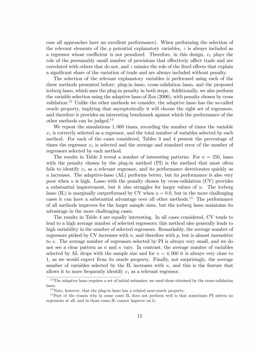
We repeat the simulations 1, 000 times, recording the number of times the variablex1 is correctly selected as a regressor, and the total number of variables selected by eachmethod. For each of the cases considered, Tables 3 and 4 present the percentage oftimes the regressor x1 is selected and the average and standard error of the number ofregressors selected by each method.The results in Table 3 reveal a number of interesting patterns. For n = 250, lasso

with the penalty chosen by the plug-in method (PI) is the method that most oftenfails to identify x1 as a relevant regressor, and its performance deteriorates quickly asu increases. The adaptive-lasso (AL) performs better, but its performance is also verypoor when u is high. Lasso with the penalty chosen by cross-validation (CV) providesa substantial improvement, but it also struggles for larger values of u. The iceberglasso (IL) is marginally outperformed by CV when u = 0.0, but in the more challengingcases it can have a substantial advantage over all other methods.14 The performanceof all methods improves for the larger sample sizes, but the iceberg lasso maintains itsadvantage in the more challenging cases.The results in Table 4 are equally interesting. In all cases considered, CV tends to

lead to a high average number of selected regressors; this method also generally leads tohigh variability in the number of selected regressors. Remarkably, the average number ofregressors picked by CV increases with n, and therefore with p, but is almost insensitiveto κ. The average number of regressors selected by PI is always very small, and we donot see a clear pattern as n and κ vary. In contrast, the average number of variablesselected by AL drops with the sample size and for n = 4, 000 it is always very close to1, as we would expect from its oracle property. Finally, not surprisingly, the averagenumber of variables selected by the IL increases with κ, and this is the feature thatallows it to more frequently identify x1 as a relevant regressor.

12The adaptive lasso requires a set of initial estimates; we used those obtained by the cross-validationlasso.13Note, however, that the plug-in lasso has a related near-oracle property.14Part of the reason why in some cases IL does not perform well is that sometimes PI selects no

regressors at all, and in those cases IL cannot improve on it.

15

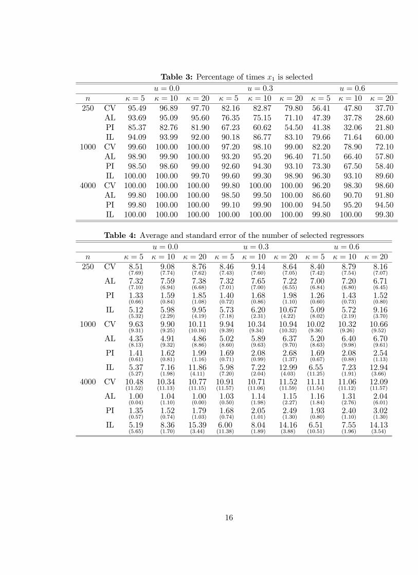
Table 3: Percentage of times x1 is selectedu = 0.0 u = 0.3 u = 0.6

n κ = 5 κ = 10 κ = 20 κ = 5 κ = 10 κ = 20 κ = 5 κ = 10 κ = 20250 CV 95.49 96.89 97.70 82.16 82.87 79.80 56.41 47.80 37.70

AL 93.69 95.09 95.60 76.35 75.15 71.10 47.39 37.78 28.60PI 85.37 82.76 81.90 67.23 60.62 54.50 41.38 32.06 21.80IL 94.09 93.99 92.00 90.18 86.77 83.10 79.66 71.64 60.00

1000 CV 99.60 100.00 100.00 97.20 98.10 99.00 82.20 78.90 72.10AL 98.90 99.90 100.00 93.20 95.20 96.40 71.50 66.40 57.80PI 98.50 98.60 99.00 92.60 94.30 93.10 73.30 67.50 58.40IL 100.00 100.00 99.70 99.60 99.30 98.90 96.30 93.10 89.60

4000 CV 100.00 100.00 100.00 99.80 100.00 100.00 96.20 98.30 98.60AL 99.80 100.00 100.00 98.50 99.50 100.00 86.60 90.70 91.80PI 99.80 100.00 100.00 99.10 99.90 100.00 94.50 95.20 94.50IL 100.00 100.00 100.00 100.00 100.00 100.00 99.80 100.00 99.30

Table 4: Average and standard error of the number of selected regressorsu = 0.0 u = 0.3 u = 0.6

n κ = 5 κ = 10 κ = 20 κ = 5 κ = 10 κ = 20 κ = 5 κ = 10 κ = 20250 CV 8.51

(7.69)9.08(7.74)

8.76(7.62)

8.46(7.43)

9.14(7.60)

8.64(7.05)

8.40(7.42)

8.79(7.54)

8.16(7.07)

AL 7.32(7.10)

7.59(6.94)

7.38(6.68)

7.32(7.01)

7.65(7.00)

7.22(6.55)

7.00(6.84)

7.20(6.80)

6.71(6.45)

PI 1.33(0.66)

1.59(0.84)

1.85(1.08)

1.40(0.72)

1.68(0.86)

1.98(1.10)

1.26(0.60)

1.43(0.73)

1.52(0.80)

IL 5.12(5.32)

5.98(2.29)

9.95(4.19)

5.73(7.18)

6.20(2.31)

10.67(4.22)

5.09(8.02)

5.72(2.19)

9.16(3.70)

1000 CV 9.63(9.31)

9.90(9.25)

10.11(10.16)

9.94(9.39)

10.34(9.34)

10.94(10.32)

10.02(9.36)

10.32(9.26)

10.66(9.52)

AL 4.35(8.13)

4.91(9.32)

4.86(8.86)

5.02(8.60)

5.89(9.63)

6.37(9.70)

5.20(8.63)

6.40(9.98)

6.70(9.61)

PI 1.41(0.61)

1.62(0.81)

1.99(1.16)

1.69(0.71)

2.08(0.99)

2.68(1.37)

1.69(0.67)

2.08(0.88)

2.54(1.13)

IL 5.37(5.27)

7.16(1.98)

11.86(4.11)

5.98(7.20)

7.22(2.04)

12.99(4.03)

6.55(11.25)

7.23(1.91)

12.94(3.66)

4000 CV 10.48(11.52)

10.34(11.13)

10.77(11.15)

10.91(11.57)

10.71(11.06)

11.52(11.59)

11.11(11.54)

11.06(11.12)

12.09(11.57)

AL 1.00(0.04)

1.04(1.10)

1.00(0.00)

1.03(0.50)

1.14(1.98)

1.15(2.27)

1.16(1.84)

1.31(2.76)

2.04(6.01)

PI 1.35(0.57)

1.52(0.74)

1.79(1.03)

1.68(0.74)

2.05(1.01)

2.49(1.30)

1.93(0.80)

2.40(1.10)

3.02(1.30)

IL 5.19(5.65)

8.36(1.70)

15.39(3.44)

6.00(11.38)

8.04(1.89)

14.16(3.88)

6.51(10.51)

7.55(1.96)

14.13(3.54)

16

In summary, for very large samples, the adaptive lasso with penalty parameter se-lected by cross validation is the preferred method; this is justified both by our simulationresults and by its oracle property. However, for small to medium samples, and especiallywith high correlation between potential explanatory variables, the adaptive lasso is out-performed by other methods. In these cases, the choice of method depends on whetherwe favor selecting the relevant regressors or having a parsimonious model. If parsimonyis paramount, the lasso with penalty parameter selected by the plug-in method is diffi -cult to beat. However, if selecting the relevant regressor is important, the iceberg lassois a safe bet and is the best method. This is particularly the case if the relevant variableis highly correlated with other potential controls because in that case the iceberg lassooutperforms the adaptive lasso even for the larger samples considered in our experiments.These results, which confirm and extend the findings of Drukker and Liu (2019), have

important implications for our work. Given that in our application we only have data on283 trade agreements,15 we cannot expect any of the methods considered to be able toprecisely identify the set of provisions that matter for trade. The task of identifying thecorrect set of explanatory variables is particularly challenging in our application becausemany of the provisions have very strong correlations with others, and there are evencases of perfect collinearity. In this challenging context, the iceberg lasso emerges asproviding a good compromise between parsimony and the ability to identify the relevantvariables. It consequently is our preferred approach.

4 Lasso Results

In this section, we present our lasso results obtained using the methods described in theprevious section. We first present results for the plug-in method before briefly discussingthe results obtained using cross-validation. We then turn to the iceberg lasso results,which themselves are based on provisions selected by the plug-in method.

4.1 Plug-in Lasso Results

Table 5 presents results for the plug-in lasso and post-lasso regressions discussed before.In column 1, we start by presenting the results of a traditional PPML estimation with adummy for the presence of a preferential trade agreement between the trading partners.This shows that we can replicate the usual finding that PTAs lead to a significant increasein trade flows in our data. Specifically, we find that the PTAs in our data increasetrade by exp (0.130) − 1 = 13.8%. Column (2) then shows the results of our first-steplasso regression, showing only the coeffi cients that the lasso finds to be non-zero. In asubsequent step, we then estimate a “post-lasso”PPML regression– a standard PPMLregression using only the provisions that were selected by the lasso in the first step.

15Note that the information on the effect of the different provisions is limited by the relatively smallnumber of PTAs that are observed. Therefore, despite having a large number of observations, weeffectively only have a small sample to identify the effect of the different provisions.

17

Table5:PPML,PPML-lasso,andpost-lassoPPMLresultsforplug-inapproach

Dependentvariable:BilateralTradeFlows(1964-2016,every4years)

PPML

PPML

PPML

Lasso

Post-lasso

PPML

PPML

Lasso

Post-lasso

(1)

(2)

(3)

(4)

(5)

(6)

(7)

PTA

0.13

0∗∗∗

−0.

030

0.08

3∗∗

(0.0

38)

(0.0

54)

(0.0

38)

EU

0.68

8∗∗∗

0.41

60.

589∗∗∗

(0.0

65)

(0.0

84)

AD14.Anti-dumping—MaterialInjury

0.17

20.

313∗∗∗

0.30

3∗∗∗

0.18

80.

343∗∗∗

(0.1

14)

(0.1

16)

(0.1

05)

CP23.CompetitionPolicy—Transparency/Coordination

0.03

10.

075

0.07

80.

011

0.04

6(0.0

56)

(0.0

56)

(0.0

54)

SUB12.Subsidies—Discipline(general)

0.00

80.

099∗

0.10

8∗∗

(0.0

52)

(0.0

55)

TBTprovisions:

TBT2.MutualRecognition

0.08

40.

073

0.06

8(0.0

93)

(0.0

94)

TBT7.TechnicalReg’s:useInternationalStandards

0.03

40.

111

0.12

10.

055

0.10

6(0.0

80)

(0.0

82)

(0.0

77)

TBT33.Standards:useRegionalStandards

0.06

70.

046

0.05

00.

039

0.03

9(0.0

66)

(0.0

66)

(0.0

51)

TradeFacilitationprovisions:

TF41.HarmonizationandCommonLegalFramework

0.03

80.

550∗∗∗

(0.1

26)

TF42.CustomsandOtherDutiesCollection

0.22

70.

354∗∗∗

0.35

2∗∗∗

(0.1

21)

(0.1

21)

TF45.IssuanceofProofofOrigin

0.02

20.

076∗∗∗

0.09

6∗∗

0.01

60.

079∗∗∗

(0.0

29)

(0.0

43)

(0.0

28)

Notes:GravityestimatesareobtainedusingPPMLwithexporter-time,importer-time,andexporter-importerFEs.

Thenumberof

observationsis194,092.Columnslabelled“PPMLPost-lasso”reportPPMLcoefficientsforallvariablesselectedbyapluginlassomethod

inapriorstep.Thedifferencebetweencolumns2-3and6-7isthatthelatterincludestheEUdummyinthelassostepasapossible

predictortobeselected.AllothercolumnsreportfurtherexperimentsusingPPML.PPMLcluster-robuststandarderrorsarereportedin

parentheses.*p<0.10,**

p<.05,***p<.01.

18

Using the plug-in approach, the lasso selects a small number of trade agreementprovisions related to anti-dumping, competition policy, domestic subsidies, technicalbarriers to trade (TBT), and trade facilitation. Broadly speaking, these variables allcan be rationalized as having intuitive effects on trade. The selected anti-dumping,competition policy, and subsidy provisions all create more certainty as to how disciplinaryinvestigations and proceedings will be carried out in these various policy areas. Thisincreased certainty may increase entry by foreign exporting firms. The inclusion ofprovisions related to technical barriers to trade and trade facilitation is likewise intuitive,but the selection of TF45, which facilitates obtaining certificates of origin, seems ofparticular note in that it highlights the costs of complying with rules of origin.The corresponding post-lasso PPML results, shown in column (3), finds that some of

the selected provisions have large effects when estimated in the conventional way. For ex-ample, the inclusion of anti-dumping provision AD14, which requires that anti-dumpingproceedings establish “material injury”to domestic producers, is associated with an in-crease in trade flows of about 36.8% (exp (0.313) − 1 = 0.368). Even larger effects arefound for having trade facilitation provisions that regulate customs and other dutiescollection (TF42), which has an estimated effect of 42.5% (exp (0.354) − 1 = 0.425).Interestingly, not all of the provisions selected by the lasso step are found to be statisti-cally significant in the post-lasso step. This apparent contradiction arises for two reasons.First, the lasso focuses on the implications for model fit when a variable is not included,which is not the same as testing whether its coeffi cient is statistically different from zero.Second, because the lasso shrinks all coeffi cients towards zero simultaneously, it reducesthe influence of the collinearity between them and can allow individual provisions thatare not significant in the conventional regressions to speak more loudly.In column (4), we re-estimate the model using the same covariates as column (3) but

now re-adding our original PTA dummy from column 1. In this case, the coeffi cient onPTA captures any effect on trade flows that is not already captured by the 8 provisionvariables that were selected by the lasso. With this in mind, we take the insignificantand near-zero coeffi cient on PTA in column (4) as an encouraging indication that theselected provisions completely explain the average PTA effect estimated in column (1).Next, column (5) returns to our original simple model from column (1) but adds a

second dummy variable for the EU agreement. Our reasons for treating the EU sepa-rately from other agreements are three-fold. First, we suspect that not all of the EU’sefforts to promote trade are captured in how their provisions variables are coded in ourdata. There could also be unobserved effects that are channeled through the EU’s sec-ondary law process, in which the EU’s governing institutions are empowered to pass newregulations and directives on an ongoing basis. Second, our provisions data does notinclude agreements that are no longer in effect. For the most part, the agreements thatcannot be included are EU pre-accession agreements, which obviously are subsumed bythe EU agreement once each new member joins the EU. As discussed in Section 2, wedeal with this data issue in practice by dropping all observations associated with obsoleteagreements. Nonetheless, this could lead to biased estimates of the EU agreement andthe provisions associated with it. Third, the EU has in place six of the eight provisions

19

selected in column 2 (all except AD14 and TBT7); thus, we want to make sure we arenot simply picking up an “EU effect”in the provisions that are selected.As the PPML results in column (5) show, the estimated EU effect is large, several

times that of non-EU PTAs in fact. However, the more important exercise is in column(6), where we now treat the EU as a possible predictor in the lasso. Because the EUis indeed selected as being an important predictor of changes in trade flows, the valueof this exercise is that the selection of other predictors is solely based on informationfrom other agreements aside from the EU. Consequently, the set of provision variablesselected by the lasso is now slightly different than in column (2), adding TF41 (whichcalls for harmonization of customs procedures) but losing TBT2, SUB12, and TF42.Notably, the post-lasso estimates in column (7) find TF41 to be highly significant bothstatistically and economically, with an estimated effect of exp (0.550)−1 = 73.3%. Giventhe possible issues with the EU we have outlined, this last set of provision variables isour preferred set to work with in the subsequent iceberg lasso analysis.

4.2 Cross-Validation Lasso Results

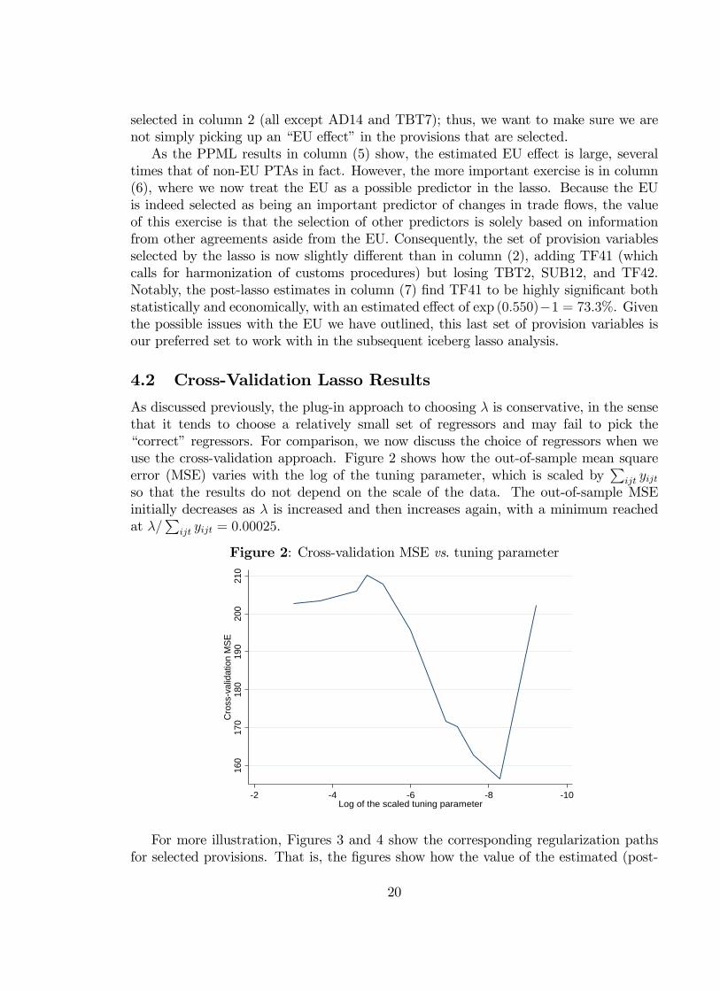
As discussed previously, the plug-in approach to choosing λ is conservative, in the sensethat it tends to choose a relatively small set of regressors and may fail to pick the“correct”regressors. For comparison, we now discuss the choice of regressors when weuse the cross-validation approach. Figure 2 shows how the out-of-sample mean squareerror (MSE) varies with the log of the tuning parameter, which is scaled by

∑ijt yijt

so that the results do not depend on the scale of the data. The out-of-sample MSEinitially decreases as λ is increased and then increases again, with a minimum reachedat λ/

∑ijt yijt = 0.00025.

Figure 2: Cross-validation MSE vs. tuning parameter

160

170

180

190

200

210

Cro

ss­v

alid

atio

nM

SE

­10­8­6­4­2Log of the scaled tuning parameter

For more illustration, Figures 3 and 4 show the corresponding regularization pathsfor selected provisions. That is, the figures show how the value of the estimated (post-

20

lasso) coeffi cient on the selected provisions changes as we vary λ. As expected, fewerprovisions are selected as we increase λ. At the optimal value of λ/

∑ijt yijt = 0.00025,

our cross-validation approach selects 124 provisions to have non-zero effects, which ismany more than what we found using our plug-in approach.16

Note, however, that it is not necessarily the case that the set of provisions selectedat lower levels of λ includes the set of provisions selected at higher levels. For example,Figure 3 shows that provision AD14, which was one of the provisions selected by ourplug-in approach, is only selected for higher values for λ. Intuitively, as we lower λ,more provisions are selected and some of these are correlated with provision AD14. Thisthen implies that adding AD14 itself does not lead to significant improvements in out-of-sample forecasts during cross-validation and hence it is no longer selected. It is onlywhen the provisions correlated with AD14 are purged from the model as λ increases thatAD14 on its own gains predictive power and is included. That said, for higher values ofλ, we generally see a close correspondence between the results along the regularizationpath indicated in Figures 3 and 4 and those that we found earlier using the plug-inmethod.Overall, Figures 3 and 4 show that our two approaches to selecting λ lead to very

different sets of trade agreement provisions being selected. While some provision, such asCP23 or SUB12 are selected by both approaches, others, such as AD14, are only selectedby the plug-in method, and many provisions are only selected using cross-validation, suchas anti-dumping provision AD05. Furthermore, we also see in Figures 3 and 4 that manyof the estimated effects for the provisions that are selected are too large in absolutemagnitude to be plausible when interpreted on their own. These observations reflect theknown shortcomings of the cross-validation approach that we stated earlier and foundsupport for in our simulations.

4.3 Iceberg Lasso Results

As previously mentioned, we cannot be certain whether the variables selected by thelasso have a causal effect on trade, or are simply highly correlated with the variablesthat have a causal effect. In this section, we investigate this issue further by carryingout the iceberg lasso analysis we proposed earlier. That is, for each of the provisionsfrom our preferred set of estimates (those from the last column of Table 5), we run anadditional plug-in lasso regression where we regress each selected provision on all of theprovisions excluded by our first-stage lasso. As discussed, the purpose of these auxiliaryregressions is to construct bundles of provisions that, at least when combined together,are likely to have a causal impact on trade flows when included in trade agreements.As we have noted, the reader should be cautioned that we will not be able to say withhigh certainty whether a given provision is important for promoting trade but, as wewill see, this method gives us significantly increased parsimony versus instead relying oncross-validation. Furthermore, as we have seen from our simulations, it should also giveus more confidence in the results.16In each panel of the figure, the second-to-last set of estimates corresponds to the 124 variables

selected by the cross-validation method.

21

Figure3:Regularizationpathforselectedprovisions(AD,ET,CM,STE,SUB,ENV,LM,andMIG)

22

Figure4:Regularizationpathforselectedprovisions(IPR,TBT,SPS,SER,ROR,TF,INV,MOC,andPP)

23

Table 6 presents the results of our iceberg lasso analysis. The first two rows of Table 6list each of the six provisions selected by the first-stage plug-in lasso when the EU dummyis included, as well as their estimated impact on trade flows from column (6) of Table 5.The subsequent rows of Table 6 report all provisions that were not selected by the lassoin the first step but are identified in the second step of the iceberg lasso; we also reportthe correlation of each of these provisions with the selected provision in the first row.Finally, the last row reports the R2 of the regression of each selected provision on thecorresponding correlated provisions. For example, column (1) shows that antidumpingprovision AD14 is highly correlated with two further antidumping provisions (AD06 andAD08) as well as with one provision on environmental protection (ENV42);17 the R2 ofthe regression of AD14 on these three provisions is 0.95.

Table 6: Iceberg lasso results(1) (2) (3) (4) (5) (6)AD14 CP23 TBT07 TBT33 TF41 TF45(+41%) (+4.7%) (+11.2%) (+4%) (+73.3%) (+8.2%)AD06 (0.97) AD06 (0.46) AD06 (0.54) AD06 (0.48) AD05 (0.89) AD11 (0.09)AD08 (0.97) AD08 (0.46) AD08 (0.54) AD08 (0.48) CP15 (0.73)ENV42 (0.97) CP22 (0.78) ENV42 (0.54) AD12 (-0.11) ET03 (0.51)

CP24 (0.89) ENV44 (0.06) ENV42 (0.48) SUB10 (0.25)ENV42 (0.46) SPS21 (0.23) ENV44 (-0.01) SUB11 (0.28)ET41 (0.16) SUB07 (0.08) INV24 (0.11) TF44 (0.98)IPR42 (-0.00) TBT15 (0.73) IPR71 (-0.08)IPR55 (-0.01) TBT34 (0.94) IPR103 (-0.11)IPR63 (-0.00) IPR107 (-0.12)IPR74 (-0.01) MOC26 (-0.10)PP08 (0.08) SPS21 (0.19)SPS21 (0.17) SUB04 (-0.11)STE31 (0.57) SUB07 (0.07)TBT02 (0.56) TBT05 (0.61)TBT15 (0.37) TBT06 (0.98)TBT29 (0.56) TBT15 (0.69)TF42 (0.56) TBT32 (0.61)TF44 (0.38) TBT34 (0.53)

0.95 0.83 0.89 0.97 0.80 0.96

Notes: Table shows PTA provisions associated with increases in bilateral trade flows (row 1),

together with the estimated increase in trade flows (row 2), as well as other provisions that predict

the provision in row 1 (rows 3-20; numbers in brackets are raw correlations with the provision

from line 1). The last row displays the R2 of the regression of each selected provision on the

corresponding correlated provisions.

The results in Table 6 show that the iceberg-lasso identifies 43 provisions that arelikely to be associated with increased trade. This finding contrasts with the 124 provi-sions identified by the cross-validation lasso, and the 6 provisions selected by the plug-inlasso. Therefore, as in the simulations in the preceding section, the iceberg lasso appears

17In our data, ENV42 is perfectly colinear with AD06 and AD08.

24

to provide a good compromise between the cross-validation lasso, which selects so manyprovisions that makes it diffi cult to interpret its results, and the plug-in lasso, which islikely to miss important provisions.As noted above, we find that provision AD14 is correlated other antidumping pro-

visions; this correlation is not surprising because all these provisions fulfill a similarpurpose, which is to increase transparency in the use of antidumping duties. In thatsense, one conclusion to be drawn from this exercise is that antidumping provisions arelikely to increase trade flows, although we cannot say which of them has the biggesteffect. Table 6 shows that, more surprisingly, AD14 is also strongly correlated withENV42. This correlation seems to be due to what might be called a template effect,that is, the tendency of important trading blocs such as the EU and the US to usesimilar provisions in all their agreements. For example, most agreements signed by theEU include provisions on antidumping and the environment, hence leading to a highcorrelation between the corresponding provisions in our data.Template effects may also be important for understanding the variables highly corre-

lated with the selected TBT provisions, TBT07 and TBT33. Indeed, some of the sameanti-dumping and environmental provisions that were found to be correlated with AD14show up here as well (AD6, AD8, ENV42). That said, the strongest correlations in thesecases are with other TBT provision such as TBT06, TBT15 and TBT34. This is notsurprising as these provisions also relate to the use of international standards. Thus, itseems likely that provisions encouraging the use of international standards in the areaof technical barriers to trade are likely to be behind the trade increases associated withprovisions TBT07 and TBT33, although we cannot say which of the individual TBTprovisions is driving the observed effect.The lasso also selects two provisions that reduce the administrative burden resulting

from compliance with rules of origin and other customs procedures (TF41 and TF45),which are estimated to have a very large trade increasing effect (over 70% for TF41).Table 6 also indicates that other trade facilitation provisions are correlated with someof the provisions selected by the lasso; this is true both for TF45 and CP23. Thus,our results suggest that trade facilitation procedures are likely to be associated withsignificant trade flow increases.Finally, we find that provision CP23, which serves to promote transparency in com-

petition policy, is correlated with some of the previously identified types of provisions,as well as with two further provisions on competition policy (CP22 and CP24). Thus, itseems likely that the presence of provisions on competition policy is behind the observedtrade increasing effect of CP23, although we are again unable to say which provisionexactly is driving this effect.The iceberg lasso also identifies provisions from other areas that help predict the

provisions identified in the first step. For example, provisions in policy areas such asintellectual property rights and sanitary and phytosanitary measures are related bothto CP23 and TBT33, but these types of provisions are associated with smaller rawcorrelations. By the logic of the lasso, it is likely that these provisions are informative forpredicting the presence of CP23 and TBT33 in a relatively small number of agreementswhere other provisions with higher raw correlations are not found.

25

In summary, although it is not possible to identify with certainty which provisionsare most important for increasing trade, our results allow us to find a relatively smallbundle of provisions that are likely to have the desired effect. In particular, provisionsrelated to TBTs, antidumping, trade facilitation, and competition policy are likely toenhance the trade-increasing effect of trade agreements.

5 Conclusions

In this paper, we have proposed new methods for assessing the impact of individual tradeagreement provisions on trade flows. While other work in this area has relied on summarymeasures of agreement depth or on specific provision bundles of interest, our approachis instead to study the rich provision content of PTAs as a variable selection problem.By combining the three-way PPML estimator that is popular in the study of PTAs withlasso methods for variable selection, we are able to identify which of the many provisionsin our data set should be treated as relevant for affecting trade flows. Using our preferredmethod, a two-step “iceberg lasso”approach, we identify a relatively parsimonious setof 43 provisions that are most likely to impact trade. While these 43 provisions span arange of policy areas, our results generally support the conclusion that a select numberof provisions related to anti-dumping, competition policy, technical barriers to trade,and trade facilitation are most effective at promoting trade as compared to other typesof provisions that appear in PTAs.We need to be clear that interpreting these results requires some important caveats.

We know that it is possible that our preferred method may fail to discover importanttrade-promoting provisions, and it is almost certain to lead to the inclusion of provisionsthat are not relevant. At present, we are not able to quantify either type of uncer-tainty. Developing metrics that can be used to guide researcher confidence represents animportant avenue for future research.In terms of broader applications, our methods are not limited to just PTAs or even

just to trade. There are many other contexts in which the iceberg lasso method wehave introduced could be a helpful tool for any researcher wishing to determine whichof a large number of variables are worth focusing on as most relevant for the outcome.Furthermore, by integrating the lasso into a nonlinear model with high-dimensional fixedeffects, we show how variable selection and other related machine learning approachescan be utilized in much more generalized settings than what had been possible previously.

26

Appendix

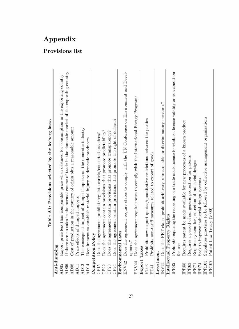
Provisions listTableA1:Provisionsselected

bytheiceberglasso

Anti-dumping

AD05

Exportpricelessthancomparablepricewhendestinedforconsumptionintheexportingcountry

AD06

Iftherearenosalesinthenormalcourseoftradeinthedomesticmarketoftheexportingcountry

AD08

Costofproductioninthecountryoforiginplusareasonableamount

AD11

Priceeffectsofdumpedimports

AD12

Theconsequentimpactofdumpedimportsonthedomesticindustry

AD14

Requirementtoestablishmaterialinjurytodomesticproducers

Com

petitionPolicy

CP15

Doestheagreementprohibit/regulatecartels/concertedpractices?

CP22

Doestheagreementcontainprovisionsthatpromotepredictability?

CP23

Doestheagreementcontainprovisionsthatpromotetransparency?

CP24

Doestheagreementcontainprovisionsthatpromotetherightofdefense?

EnvironmentalLaws

ENV42

DoestheagreementrequirestatestocomplywiththeUNConferenceonEnvironmentandDevel-

opment?

ENV44

DoestheagreementrequirestatestocomplywiththeInternationalEnergyProgram?

ExportTaxes

ET03

Prohibitsnewexportquotas/quantitativerestrictionsbetweentheparties

ET41

Prohibitsnon-tariffmeasuresrelatedtoexportofgoods

Investment

INV24

DoestheFETclauseprohibitarbitrary,unreasonableordiscriminatorymeasures?

IntellectualPropertyRights

IPR42

Prohibitsrequiringtherecordingofatrademarklicensetoestablishlicensevalidityorasacondition

foruse

IPR55

Requirespatentbemadeavailablefornewprocessesofaknownproduct

IPR63

Requiresaperiodofsuigenerisprotectionforpatents

IPR71

Requiressystem

forprotectionofindustrialdesigns

IPR74

Seektoimproveindustrialdesignsystems

IPR103

Stipulatespracticestobefollowedbycollectivemanagementorganizations

IPR107

PatentLaw

Treaty(2000)

27

TableA1(cont’d):Provisionsselected

bytheiceberglasso

MovementofCapital

MOC26

Doesthetransferprovisionexplicitlyexclude“goodfaith”andnon-discriminatoryapplicationof

itslawsrelatedtopreventionofdeceptiveandfraudulentpractices?

PublicProcurement

PP08

DoestheagreementcontainexplicitprovisionsonMFNtreatmentofthirdparties?

SanitaryandPhytosanitaryMeasures

SPS21

B.RiskAssessment:Istherereferencetointernationalstandards/procedures?

State-Owned

Enterprises

STE31

Doestheagreementprohibitanti-competitivebehaviorofstateenterprises?

Subsidies

SUB04

Doestheagreementprohibitorregulatelocal-contentsubsidies?

SUB07

Doestheagreementintroduceanyceilingtopermittedsubsidies?

SUB10

Doestheagreementincludeanyspecificregulationoffisheriessubsidies?

SUB11

Doestheagreementincludeanyspecificdisciplineforpublicservices?

SUB12

Doestheagreementincludeanyotherspecificdisciplineforcertainsectorsorobjectives?

TechnicalBarrierstoTrade

TBT02

B.TechnicalRegulations-Ismutualrecognitioninforce?

TBT05

B.TechnicalRegulations-Aretherespecifiedexistingstandardstowhichcountriesshallharmonize?

TBT06

B.TechnicalRegulations-Istheuseorcreationofregionalstandardspromoted?

TBT07

B.TechnicalRegulations-Istheuseofinternationalstandardspromoted?

TBT15

C.ConformityAssessment-Istheuseofinternationalstandardspromoted?

TBT29

A.Standards-Ismutualrecognitioninforce?

TBT32

A.Standards-Aretherespecifiedexistingstandardstowhichcountriesshallharmonize?

TBT33

A.Standards-Istheuseorcreationofregionalstandardspromoted?

TBT34

A.Standards-Istheuseofinternationalstandardspromoted?

TradeFacilitationandCustom

sTF41

Doestheagreementrequirecustomsharmonizationandacommonlegalframework?

TF42

Doestheagreementregulatecustomsandotherdutiescollection?

TF44

Dotradefacilitationprovisionssimplifyrequirementsforproofoforigin?

TF45

Doestradefacilitationprovisionssimplifyprocedurestoissueproofoforigin?

28

More Details on HDFE-PPML-Lasso Estimation

The minimization problem that defines the three-way PPML-lasso is

(α̂, γ̂, η̂, β̂) := arg minα,γ,η,β

1

n

∑i,j,t

exp(x′ijtβ + αit + γjt + ηij)

− 1

n

∑i,j,t

yijt(x′ijtβ + αit + γjt + ηij

)+

1

n

p∑k=1

φ̂kλ|βk|. (3)

The first-order conditions (FOCs) for this problem are

α̂it :1

n

∑j

yijt − µ̂ijt = 0, ∀i, t,

γ̂jt :1

n

∑i

yijt − µ̂ijt = 0, ∀j, t,

η̂ij :1

n

∑t

yijt − µ̂ijt = 0, ∀i, j,

β̂k :1

n

∑i,j,t

(yijt − µ̂ijt

)xijt,k +

1

nφ̂kλsign(β̂k) = 0, k = 1...p,

where µ̂ijt denotes µijt evaluated at α̂, γ̂, η̂, β̂. Notice that the penalty only affects theFOCs for the main covariates of interest. The FOCs for the fixed effects are exactly thesame as they would be in unpenalized PPML. That said, further simplification is stillneeded because it is generally not possible to estimate all of the parameters directly,with or without the penalty. Instead, we first need to “concentrate out”the fixed effectparameters. That is, instead of minimizing (3) over all of the parameters, we treatα̂it(β̂), γ̂it(β̂), and η̂it(β̂) as functions of β̂ that are implicitly defined by their FOCs.The resulting “concentrated”minimization problem is

β̂ := arg minβ

1

n

∑i,j,t

exp(x′ijtβ + α̂it (β) + γ̂jt (β) + η̂ij (β)

)− 1

n

∑i,j,t

yijt(x′ijtβ + α̂it (β) + γ̂jt (β) + η̂ij (β)

)+

1

n

p∑k=1

φ̂kλ|βk|, (4)

such that β is now the only argument we need to solve for. The FOC for each β̂kassociated with this modified problem is:

β̂k :1

n

∑i,j,t

(yijt − exp

(x′ijtβ̂ + α̂it

(β̂)

+ γ̂jt

(β̂)

+ η̂ij

(β̂)))

x̃ijt,k +1

nφ̂kλ sign(β̂k) = 0,

where

x̃ijt,k := xijt,k +dα̂it,kdβ

+dγ̂it,kdβ

+dη̂ij,kdβ

(5)

29

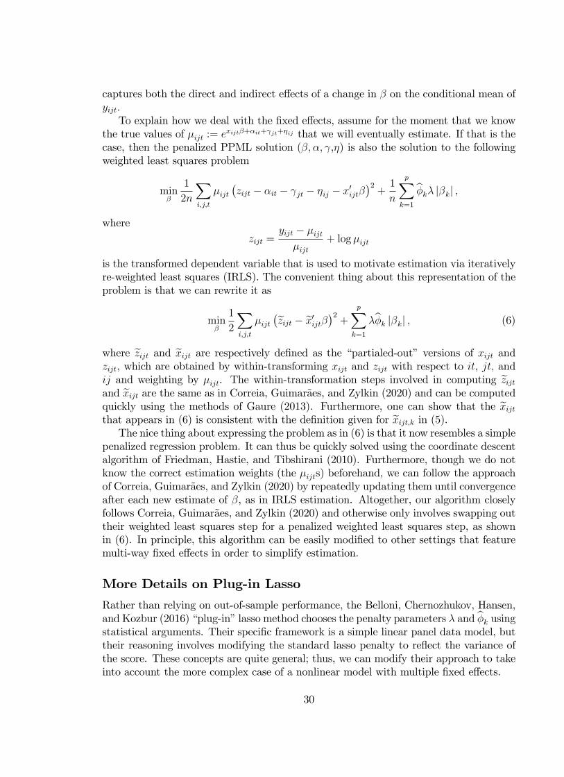
captures both the direct and indirect effects of a change in β on the conditional mean ofyijt.To explain how we deal with the fixed effects, assume for the moment that we know

the true values of µijt := exijtβ+αit+γjt+ηij that we will eventually estimate. If that is thecase, then the penalized PPML solution (β, α, γ,η) is also the solution to the followingweighted least squares problem

minβ

1

2n

∑i,j,t

µijt(zijt − αit − γjt − ηij − x′ijtβ

)2+

1

n

p∑k=1

φ̂kλ |βk| ,

wherezijt =

yijt − µijtµijt

+ log µijt

is the transformed dependent variable that is used to motivate estimation via iterativelyre-weighted least squares (IRLS). The convenient thing about this representation of theproblem is that we can rewrite it as

minβ

1

2

∑i,j,t

µijt(z̃ijt − x̃′ijtβ

)2+

p∑k=1

λφ̂k |βk| , (6)

where z̃ijt and x̃ijt are respectively defined as the “partialed-out” versions of xijt andzijt, which are obtained by within-transforming xijt and zijt with respect to it, jt, andij and weighting by µijt. The within-transformation steps involved in computing z̃ijtand x̃ijt are the same as in Correia, Guimarães, and Zylkin (2020) and can be computedquickly using the methods of Gaure (2013). Furthermore, one can show that the x̃ijtthat appears in (6) is consistent with the definition given for x̃ijt,k in (5).The nice thing about expressing the problem as in (6) is that it now resembles a simple

penalized regression problem. It can thus be quickly solved using the coordinate descentalgorithm of Friedman, Hastie, and Tibshirani (2010). Furthermore, though we do notknow the correct estimation weights (the µijts) beforehand, we can follow the approachof Correia, Guimarães, and Zylkin (2020) by repeatedly updating them until convergenceafter each new estimate of β, as in IRLS estimation. Altogether, our algorithm closelyfollows Correia, Guimarães, and Zylkin (2020) and otherwise only involves swapping outtheir weighted least squares step for a penalized weighted least squares step, as shownin (6). In principle, this algorithm can be easily modified to other settings that featuremulti-way fixed effects in order to simplify estimation.

More Details on Plug-in Lasso

Rather than relying on out-of-sample performance, the Belloni, Chernozhukov, Hansen,and Kozbur (2016) “plug-in”lasso method chooses the penalty parameters λ and φ̂k usingstatistical arguments. Their specific framework is a simple linear panel data model, buttheir reasoning involves modifying the standard lasso penalty to reflect the variance ofthe score. These concepts are quite general; thus, we can modify their approach to takeinto account the more complex case of a nonlinear model with multiple fixed effects.

30

The key condition in choosing these penalty parameters is that they should satisfythe following inequality for all k:

λφ̂kn≥ c

∣∣∣∣∣ 1n∑i,j,t

(yijt − exp(x′ijtβ + αit + γjt + ηij))x̃ijt,k

∣∣∣∣∣ ∀k, (7)

for some c > 1. Intuitively,∣∣∣∣∣ 1n∑i,j,t

(yijt − exp(x′ijtβ + αit + γjt + ηij))x̃ijt,k

∣∣∣∣∣is the absolute value of the score for βk.When evaluated at βk = 0, it tells us to whatdegree moving each βk away from zero will affect the fit of the model. If it does notproduce a suffi cient improvement in fit as compared to the penalty λφ̂k, then regressorxijt,k will not be selected.Next, set

φ̂2

k =1

n

∑i,j

(∑t

x̃ijt,kε̂ijt

)2

=1

n

∑i,j

∑t

∑t′

x̃ijt,kx̃ijt′,k ε̂ijt̂εijt′ ,

where ε̂ijt = yijt−exp(x′ijtβ̂+ α̂it+ γ̂jt+ η̂ij), but can also be obtained as ε̂ijt = µ̂ijt(z̃ijt−x̃′ijtβ̂). By inspection, this expression provides an estimate of the variance of the scorefor βk under the assumption that errors are correlated over time within the same pair,as is commonly assumed in this context. Provided there is weak temporal dependence(in the sense described by Hansen, 2007), φ̂

2

k − φ2k = op(1) uniformly in k, where φ2

k is

the analogue of φ̂2

k evaluated at the true values of εijt. By choosing φ̂k in this way weensure that the score for βk when evaluated at zero must be large as compared to itsstandard deviation in order for regressor k to be selected.The choice of λ then involves setting a value that is suffi ciently large that the statis-

tical probability an irrelevant regressor is selected is small. By the maximal inequalityfor self-normalized sums (see Jing, Shao, and Wang, 2003), it follows that

Pr(φ̂−1

k1√n

∑i,j,t x̃ijt,kεijt ≥ m

)Pr (N(0, 1) ≥ m)

= o(1),

for |m| = o(n1/6), thus establishing a bound for the tails of the normalized sum. Thissuggests that by choosing a λ that is suffi ciently large to dominate a p-dimensional stan-dard normal, the inequality in (7) is satisfied. Hence, following Belloni, Chernozhukov,Hansen, and Kozbur (2016), we set

λ = λplug = 2c√nΦ−1 (1− γ/2p) ,

where c = 1.1 and γ = 0.1/ log(n).

31

As discussed in the main text, after the lasso step, we then perform an unpenalizedPPML estimation using the selected covariates, a so-called “post-lasso”regression. Letβ̂PL be the estimator of the parameters associated with the s selected covariates. Suchan estimator is said to have the “oracle property”if the asymptotic distribution of β̂PLcoincides with that of the estimator we would obtain if we knew exactly which coeffi cientswere equal to zero, i.e., for large enough samples we would have β̂PL,k = 0 if and onlyif βk = 0 for k = 1, ..., p. Hence, for estimators with the oracle property, asymptoticallythe post-lasso model is indeed the right model. In general, the lasso does not satisfy theoracle property. Nevertheless, under some additional regularization conditions, the useof the plug-in lasso method just described ensures the following “near-oracle”propertyfor β̂PL, ∥∥∥β̂PL − β∥∥∥

1= Op

(√s2 max (log n, log p)

n

),

and hence the post-lasso estimates are consistent at a rate that differs from the oraclerate only up to the log factor max (log n, log p).In practice, the plug-in lasso method only requires adding one additional step to the

procedure used for the estimation of the PPML-lasso with high-dimensional fixed effectsdescribed before. Though the φ̂k penalty terms are not known beforehand, they, too,can be iterated on in the same fashion as µijt. Simply use the most recent values of ε̂ijtin each iteration to construct new values for φ̂k.

More Details on Cross-Validation

As discussed in the main text, the idea behind cross-validation (CV) is to repeatedly holdout a subset of the sample during estimation and then use it to validate the resultingestimates. In our setup, rather than holding out observations in an unstructured way,we keep together all observations for which a given agreement is in effect, and hold outsubsets of agreements. Doing so allows us to obtain estimates for the all the fixed effectsin the model.To describe the implementation of CV, suppose that the observations associated with

trade agreements are partitioned into G subsets. Each resulting hold-out sample g willhave ng observations, where ng is the number of observations associated with agreementsthat are held out in partition g. Because our variables of interest are all dummies, aproblem that may occur is that over some subsamples some regressors may not be present,but that is less likely to happen when G is large.The CV approach sets all regressor-specific penalty weights φ̂k equal to 1. Let β̂L,g(λ)

be the lasso estimator obtained via the minimization of (4) when holding out the ngobservations contained in partition j. Define the CV bandwidth as

λCV = arg minλ∈Λ

1

G

G∑g=1

1

ng

∑(i,j,t)∈g

(yijt

− exp(x′ijtβ̂L,g(λ) + αit

(β̂L,g(λ)

)+ γjt

(β̂L,g(λ)

)+ ηij

(β̂L,g(λ)

)))2

.

32

Since λCV is based on the minimization of the average MSE over different subsamples, weexpect it to deliver a much more lenient variable selection. There is some disagreementover whether dummy variables, such as the ones used in our application, should bestandardized before applying the CV lasso. This consideration is in contrast to the plug-in lasso, since standardization of the covariates simply causes the φ̂k terms to be re-scaledwithout otherwise affecting estimation in that case. We have computed CV lasso resultswith and without first standardizing and found that the results with standardization arenoticeably more similar to the plug-in lasso results. Thus, our preference is to work withstandardized dummy covariates.

References

Anderson, J. and E. Van Wincoop (2003). “Gravity with gravitas: A solution to theborder puzzle,”American Economic Review, 93, 170-192.

Baier, S.L. and J.H. Bergstrand (2007). “Do free trade agreements actually increasemembers’international trade?,”Journal of International Economics, 71, 72-95.

Baier, S.L., J.H. Bergstrand, and M.W. Clance (2018). “Heterogeneous effects of eco-nomic integration agreements,”Journal of Development Economics, 135, 587-608.

Baier, S.L., J.H. Bergstrand, and M. Feng (2014). “Economic integration agreementsand the margins of international trade,”Journal of International Economics, 93,339-350.

Baier, S.L, Y.V. Yotov, T. Zylkin (2019). “On the widely differing effects of freetrade agreements: Lessons from twenty years of trade integration,” Journal ofInternational Economics, 116, 206-228.

Belloni, A., D. Chen, V. Chernozhukov, and C. Hansen (2012). “Sparse models andmethods for optimal instruments with an application to eminent domain,”Econo-metrica, 80, 2369-2429.

Belloni A., V. Chernozhukov, C. Hansen (2014). “Inference on treatment effects afterselection among high-dimensional controls,”Review of Economics Studies, 81, 608-650.

Belloni, A., V. Chernozhukov, C. Hansen, D. Kozbur (2016). “Inference in high dimen-sional panel models with an application to gun control,” Journal of Business &Economic Statistics, 34, 590-605.

Correia, S., P. Guimarães and T. Zylkin (2020). “Fast Poisson estimation with highdimensional fixed effects,”STATA Journal, 20, 90-115.

Dhingra, S., R. Freeman, and E. Mavroeidi (2018). “Beyond tariff reductions: Whatextra boost to trade from agreement provisions?,”LSE Centre for Economic Per-formance Discussion Paper 1532.

Drukker, D.M and D. Liu (2019). “A plug-in for Poisson lasso and a comparison ofpartialing-out Poisson estimators that use different methods for selecting the lassotuning parameters,”mimeo.

33

Fu, W. and K. Knight (2000). “Asymptotics for lasso-type estimators,” Annals ofStatistics, 28, 1356-1378.

Friedman, J., T. Hastie, and R. Tibshirani (2010). “Regularization paths for generalizedlinear models via coordinate descent,”Journal of Statistical Software, 33, 1-22.

Gaure, S (2013). “OLS with multiple high dimensional category variables,”Computa-tional Statistics & Data Analysis 66, 8-18.

Gourieroux, C., A. Monfort, A. Trognon (1984). “Pseudo maximum likelihood methods:Applications to Poisson models,”Econometrica, 52, 701-720.

Hansen, C. (2007). “Asymptotic properties of a robust variance matrix estimator forpanel data when T is large,”Journal of Econometrics, 141, 597-620.

Hastie, T., R. Tibshirani, and J.H. Friedman (2009). The elements of statistical learn-ing: Data mining, inference, and prediction. New York (NY): Springer.

Head, K. and T. Mayer (2014). “Gravity equations: Workhorse, toolkit, and cookbook,”Handbook of International Economics, Vol. 4: 131-195.

Hofmann, C., A. Osnago, M. Ruta (2017). “Horizontal depth. A new database on thecontent of preferential trade agreements,”World Bank Policy Research WorkingPaper 7981.

Jing, B.Y., Q.M. Shao, and Q. Wang (2003). “Self-normalized Cramér-type large devia-tions for independent random variables,”The Annals of Probability, 31, 2167-2215.

Kohl, T., S. Brakman, H. Garretsen (2016). “Do trade agreements stimulate interna-tional trade differently? Evidence from 296 trade agreements,”The World Econ-omy, 39, 97-131.

Larch, M., J. Wanner, Y.V. Yotov, T. Zylkin (2019). “Currency unions and trade:a PPML re-assessment with high dimensional fixed effects,”Oxford Bulletin ofEconomics and Statistics, 81, 487-510.

Mattoo, A., A. Mulabdic, and M. Ruta (2017). Trade creation and trade diversion indeep agreements. Policy Research Working Paper Series 8206, The World Bank.

Mattoo, A., N. Rocha, M. Ruta (2020). “Handbook of deep trade agreements.”Wash-ington, DC: World Bank.

Mulabdic, A., A. Osnago, and M. Ruta (2017). “Deep integration and UK-EU traderelations,”World Bank Policy Research Working Paper Series 7947.

Regmi, N. and S. Baier (2020). “Using machine learning methods to capture hetero-geneity in free trade agreements,”mimeograph.

Santos Silva, J.M.C. and S. Tenreyro (2006). “The log of gravity,”Review of Economicsand Statistics, 88, 641-658.

Stammann, A. (2018). “Fast and feasible estimation of generalized linear models withhigh-dimensional k-way fixed effects,”arXiv:1707.01815.

Tibshirani, R. (1996). “Regression shrinkage and selection via lasso,” Journal of theRoyal Statistical Society, Ser B. 59, 267-288.

34

Weidner, M., T. Zylkin (2020). “Bias and consistency in three-way gravity models,”arXiv:1909.01327.

Yotov, Y.V., R. Piermartini, J.-A. Monteiro, M. Larch (2016). An advanced guide totrade policy analysis: The structural gravity model. Geneva: World Trade Organi-zation.

Zhao, P. and B. Yu (2006). “On model selection consistency of lasso,” Journal ofMachine Learning Research, 7, 2541-2563.

Zou, H. (2006). “The adaptive lasso and its oracle properties,”Journal of the AmericanStatistical Association, 101, 1418-1429.

35