Malliavin Calculus

Matheus Grasselli Tom HurdDepartment of Mathematics & Statistics, McMaster University

Hamilton, Ontario, Canada L8S 4K1

April, 2005

1 Introduction

2 Malliavin Calculus

2.1 The Derivative Operator

Consider a probability space (Ω,F , P ) equipped with a filtration (Ft) generated by a one-

dimensional Brownian motion Wt and let L2(Ω) be the space of square integrable random

variables.

Let L2[0, T ] denote the Hilbert space of deterministic square integrable functions h : [0, T ] →

R. For each h ∈ L2[0, T ], define the random variable

W (h) =

∫ T

0

h(t)dWt

using the usual Ito integral with respect to a Brownian motion. Observe that this is a Gaussian

random variable with E[W (h)] = 0 and that, due to the Ito isometry,

E[W (h)W (g)] =

∫ T

0

h(t)g(t)dt =< h, g >L2[0,T ],

for all h, g ∈ L2[0, T ].

The closed subspace H1 ⊂ L2(Ω) of such random variables is then isometric to L2[0, T ] and

is called the space of zero-mean Gaussian random variables.

1

Now let C∞p (Rn) be the set of smooth functions f : Rn → R with partial derivatives of

polynomial growth. Denote by S the class of random variables of the form

F = f(W (h1), ...,W (hn))

where f ∈ C∞p and h1, ..., hn ∈ L2([0, T ]). Note that S is then a dense subspace of L2(Ω).

Definition 2.1 : For F ∈ S, we define the stochastic process

DtF =n∑

i=1

∂f

∂xi

(W (h1), ...,W (hn))hi(t)

One can then show that DF ∈ L2(Ω× T ).

So for we have obtained a linear operator D : S ⊂ L2(Ω) → L2(Ω×T ). We can now extend

the domain of D by considering the norm

||F ||1,2 = ||F ||L2(Ω) + ||DtF ||L2(Ω×T )

We then define D1,2 as the closure of S in the norm || · ||1,2. Then

D : D1,2 ⊂ L2(Ω) → L2(Ω× T )

is a closed unbounded operator with a dense domain D1,2.

Properties:

1. Linearity: Dt(aF + G) = aDtF + DtG, ∀F, G ∈ D1,2

2. Chain Rule: Dt(f(F )) =∑

fi(F )DtF, ∀f ∈ C∞p (R), Fi ∈ D1,2

3. Product Rule:Dt(FG) = F (DtG) + G(DtF ), ∀F, G ∈ D1,2 s.t. F and ||DF ||L2(Ω×T ) are

bounded.

Simple Examples:

1. Dt(∫ T

0h(t)dWt) = h(t)

2. DtWs = 1t≤s

2

3. Dtf(Ws) = f′(Ws)1t≤s

Exercises: Try Oksendal (4.1) (a), (b), (c), (d).

Frechet Derivative Interpretation

Recall that the sample space Ω can be identified with the space of continuous function

C([0, T ]). Then we can look at the subspace

H1 = γ ∈ Ω : γ =

∫ t

0

h(s)ds, h ∈ L2[0, T ],

that is, the space of continuous functions with square integrable derivatives. This space is

isomorphic to L2[0, T ] and is called the Cameron-Martin space. Then we can prove that∫ T

0(Dt)Fh(t)dt is the Frechet derivative of F in the direction of the curve γ =

∫ t

0h(s)ds,

that is ∫ T

0

DtFh(t)dt =d

dεF (w + εγ)|ε=0

2.2 The Skorohod Integral

Riemann Sums

Recall that for elementary adapted process

ut =n∑

i=0

Fi1(ti,ti+1](t), Fi ∈ Fti

the Ito integral is initially defined as∫ T

0

utdWt =n∑

i=0

Fi(Wti+1−Wti)

Since ε is dense in L20(Ω× T ), we obtain the usual Ito integral in L2

0(Ω× T ) by taking limits.

Alternatively, instead of approximating a general process ut ∈ L2(Ω× T ) by a step process

of the form above, we could approximate it by the step process

u(t) =n∑

i=0

1

ti+1 − ti

((

∫ ti+1

ti

E[us|F[ti,ti+1]c ]ds

)1(ti,ti+1](t)

3

and consider the Riemann sum

n∑i=0

1

ti+1 − ti

(∫ ti+1

ti

E[us|F[ti,ti+1]c ]ds

))(Wti+1

−Wti).

If these sums converge to a limit in L2(Ω) as the size of the partition goes to zero, then the

limit is called the Skorohod integral of u and is denoted by δ(u). This is clearly not a friendly

definition!

Skorohod Integral via Malliavin Calculus

An alternative definition for the Skorohod integral of a process u ∈ L2[T × Ω] is as the

adjoint to the Malliavin derivate operator.

Define the operator δ : Dom(δ) ⊂ L2[T × Ω] → L2(Ω) with domain

Dom(δ) = u ∈ L2[T × Ω] : |E(

∫ T

0

DtFutdt)| ≤ c(u)||F ||L2(Ω),∀F ∈ D1,2

characterized by

E[Fδ(u)] = E[intT0 DtFutdt]

that is,

< F, δ(u) >L2=< DtF, u >L2[T×Ω]

That is, δ is a closed, unbounded operator taking square integrable process to square integrable

random variables. Observe that E[δ(u)] = 0 for all u ∈ Domδ.

Lemma 2.0.1 :Let u ∈ Dom(δ), F ∈ D1,2 s.t. Fu ∈ L2[T × Ω]. Then

δ(Fu) = Fδ(u)−∫ T

0

DtFutdt (1)

in the sense that (Fu) is Skorohod integrals iff the right hand side belongs to L2(Ω).

Proof:Let G = g(W (G1, ..., Gn)) be smooth with g of compact support. Then from the product

rule

4

E[GFδ(u)] = E[

∫ T

0

Dt(GF )utdt]

= E[G

∫ T

0

DtFutdt] + E[F

∫ T

0

DtGutdt]

= E[G

∫ T

0

DtFutdt] + E[Gδ(Fu)]

For the next result, let us denote by L2a[T ×Ω] the subset of L2[T ×Ω] consisting of adapted

processes.

Proposition 2.0.1 : L2a[T×Ω] ⊂ Dom(δ) and δ restricted to L2

a coincides with the Ito integral.

Exercises: Now do Oksendal 2.6, 2.1 (a),(b),(c),(d), 4.1 (f), as well as examples (2.3) and (2.4).

3 Wiener Chaos

Consider the Hermite polynomials

Hn(x) = (−1)nex2/2 dn

dxne−x2/2, H0(x) = 1

which are the coefficients for the power expansion of

F (x, t) = ext− t2

2

= ex2

2 e−12(x−t)2

= ex2

2

∞∑n=0

tn

n!(dn

dtne−

12(x−t)2)|t=0

=∞∑

n=0

tn

n!Hn(x)

It then follows that we have the recurrence relation

(x− d

dx)Hn(x) = Hn+1(x).

5

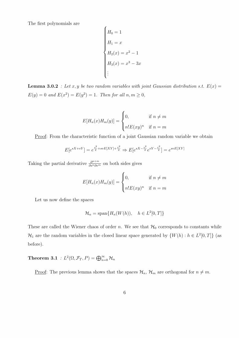
The first polynomials are

H0 = 1

H1 = x

H2(x) = x2 − 1

H3(x) = x3 − 3x

...

Lemma 3.0.2 : Let x, y be two random variables with joint Gaussian distribution s.t. E(x) =

E(y) = 0 and E(x2) = E(y2) = 1. Then for all n, m ≥ 0,

E[Hn(x)Hm(y)] =

0, if n 6= m

n!E(xy)n if n = m

Proof: From the characteristic function of a joint Gaussian random variable we obtain

E[esX+vY ] = es2

2+svE[XY ]+ v2

2 ⇒ E[esX− s2

2 evY− v2

2 ] = esvE[XY ]

Taking the partial derivative ∂n+m

∂sn∂vm on both sides gives

E[Hn(x)Hm(y)] =

0, if n 6= m

n!E(xy)n if n = m

Let us now define the spaces

Hn = spanHn(W (h)), h ∈ L2[0, T ]

These are called the Wiener chaos of order n. We see that H0 corresponds to constants while

H1 are the random variables in the closed linear space generated by W (h) : h ∈ L2[0, T ] (as

before).

Theorem 3.1 : L2(Ω,FT , P ) =⊕∞

n=0Hn

Proof: The previous lemma shows that the spaces Hn, Hm are orthogonal for n 6= m.

6

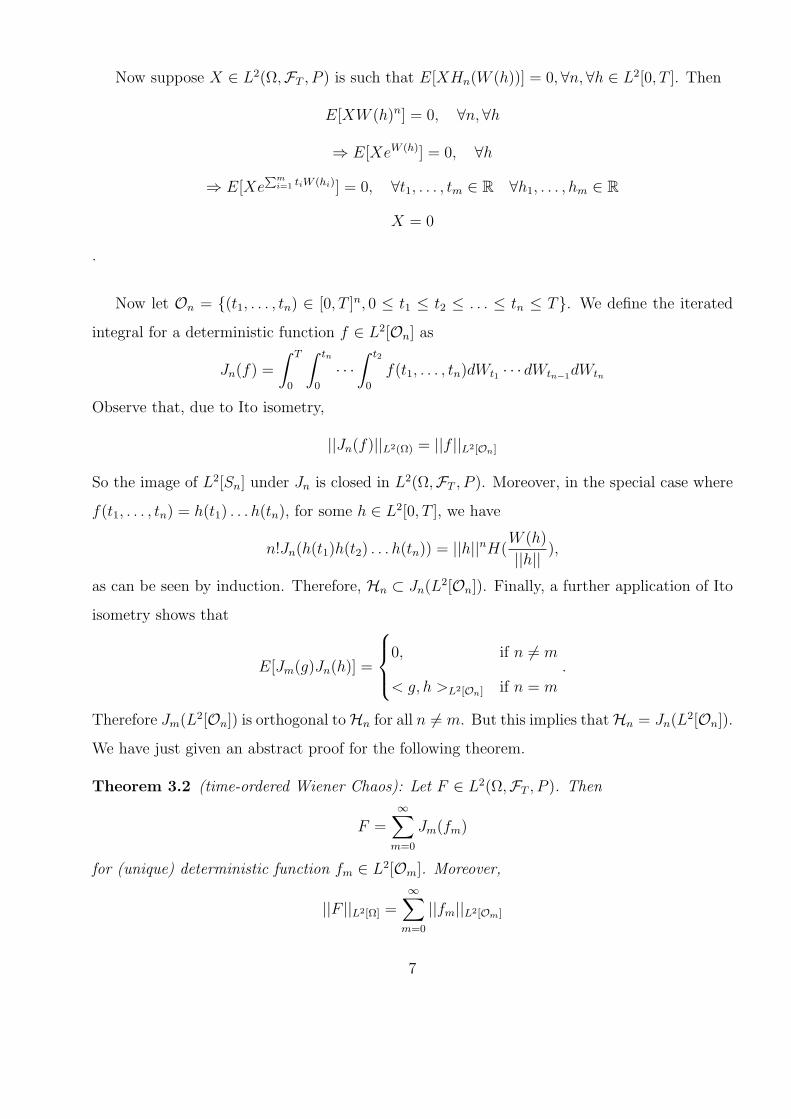
Now suppose X ∈ L2(Ω,FT , P ) is such that E[XHn(W (h))] = 0,∀n,∀h ∈ L2[0, T ]. Then

E[XW (h)n] = 0, ∀n,∀h

⇒ E[XeW (h)] = 0, ∀h

⇒ E[XePm

i=1 tiW (hi)] = 0, ∀t1, . . . , tm ∈ R ∀h1, . . . , hm ∈ R

X = 0

.

Now let On = (t1, . . . , tn) ∈ [0, T ]n, 0 ≤ t1 ≤ t2 ≤ . . . ≤ tn ≤ T. We define the iterated

integral for a deterministic function f ∈ L2[On] as

Jn(f) =

∫ T

0

∫ tn

0

· · ·∫ t2

0

f(t1, . . . , tn)dWt1 · · · dWtn−1dWtn

Observe that, due to Ito isometry,

||Jn(f)||L2(Ω) = ||f ||L2[On]

So the image of L2[Sn] under Jn is closed in L2(Ω,FT , P ). Moreover, in the special case where

f(t1, . . . , tn) = h(t1) . . . h(tn), for some h ∈ L2[0, T ], we have

n!Jn(h(t1)h(t2) . . . h(tn)) = ||h||nH(W (h)

||h||),

as can be seen by induction. Therefore, Hn ⊂ Jn(L2[On]). Finally, a further application of Ito

isometry shows that

E[Jm(g)Jn(h)] =

0, if n 6= m

< g, h >L2[On] if n = m

.

Therefore Jm(L2[On]) is orthogonal toHn for all n 6= m. But this implies thatHn = Jn(L2[On]).

We have just given an abstract proof for the following theorem.

Theorem 3.2 (time-ordered Wiener Chaos): Let F ∈ L2(Ω,FT , P ). Then

F =∞∑

m=0

Jm(fm)

for (unique) deterministic function fm ∈ L2[Om]. Moreover,

||F ||L2[Ω] =∞∑

m=0

||fm||L2[Om]

7

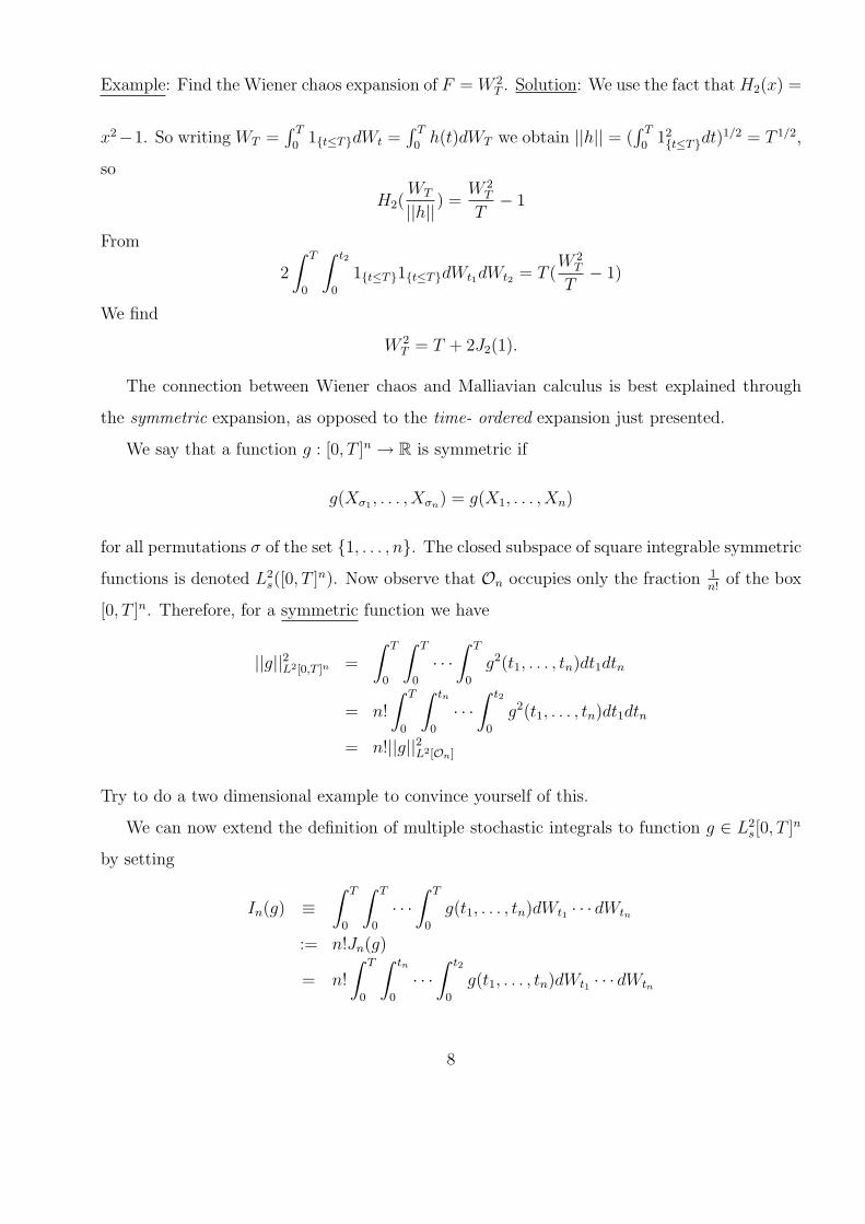
Example: Find the Wiener chaos expansion of F = W 2T . Solution: We use the fact that H2(x) =

x2−1. So writing WT =∫ T

01t≤TdWt =

∫ T

0h(t)dWT we obtain ||h|| = (

∫ T

012t≤Tdt)1/2 = T 1/2,

so

H2(WT

||h||) =

W 2T

T− 1

From

2

∫ T

0

∫ t2

0

1t≤T1t≤TdWt1dWt2 = T (W 2

T

T− 1)

We find

W 2T = T + 2J2(1).

The connection between Wiener chaos and Malliavian calculus is best explained through

the symmetric expansion, as opposed to the time- ordered expansion just presented.

We say that a function g : [0, T ]n → R is symmetric if

g(Xσ1 , . . . , Xσn) = g(X1, . . . , Xn)

for all permutations σ of the set 1, . . . , n. The closed subspace of square integrable symmetric

functions is denoted L2s([0, T ]n). Now observe that On occupies only the fraction 1

n!of the box

[0, T ]n. Therefore, for a symmetric function we have

||g||2L2[0,T ]n =

∫ T

0

∫ T

0

· · ·∫ T

0

g2(t1, . . . , tn)dt1dtn

= n!

∫ T

0

∫ tn

0

· · ·∫ t2

0

g2(t1, . . . , tn)dt1dtn

= n!||g||2L2[On]

Try to do a two dimensional example to convince yourself of this.

We can now extend the definition of multiple stochastic integrals to function g ∈ L2s[0, T ]n

by setting

In(g) ≡∫ T

0

∫ T

0

· · ·∫ T

0

g(t1, . . . , tn)dWt1 · · · dWtn

:= n!Jn(g)

= n!

∫ T

0

∫ tn

0

· · ·∫ t2

0

g(t1, . . . , tn)dWt1 · · · dWtn

8

It then follows that

E[I2n(g)] = E[n!2J2

n(g)] = n!2||g||L2[On] = n!||g||L2[0,T ]n

so the image of L2s[0, T ]n under In is closed. Also, for the particular case g(t1, . . . , tn) =

h(t1) . . . h(tn), the previous result for the time-ordered integral gives

In(h(t1) . . . h(tn)) = ||h||nHn(W (h)

||h||)

Therefore we again have that Hn ⊂ In(L2s). Moreover, the orthogonality relation between

integrals of different orders still holds, that is

E[Jn(g)Jm(h)] =

0, if n 6= m

n! < g, h > if n = m

Therefore In(L2s) is orthogonal to all Hm, n 6= m, which implies In(L2

s) = Hn.

Theorem 3.3 (symmetric Wiener chaos) Let L2(Ω,FT , P ). Then

F =∞∑

m=0

Im(gm)

for (unique) deterministic functions gm ∈ L2s[0, T ]n. Moreover, ||F ||L2(s) =

∑∞m=0 m!||gm||L2[0,T ]n

To go from the two ordered expansion to the symmetric one, we have to proceed as following.

Suppose we found

F =∞∑

m=0

Jm(fm), fm ∈ L2[On]

First extend fm(t1, . . . , tm) from Om to [0, T ]m by setting

fm(t1, . . . , tm) = 0 if (t1, . . . , tm) ∈ [0, T ]m\Om

Then define a symmetric function

gm(t1, . . . , tm) =1

m!

∑σ

fm(tσ1 , . . . , tσm)

Then

Im(gm) = m!Jm(gm) = Jm(fm)

9

Example: What is the symmetric Wiener chaos expansion of F = Wt(WT − Wt)? Solution:

Observe that

Wt(W (T )−Wt) = Wt

∫ T

t

dWt2

=

∫ T

t

∫ t

0

dWt1dWt2

=

∫ T

0

∫ t2

0

1t1<t<t2dWt1dWt2

Therefore F = J2(1t1<t<t2). To find the symmetric expansion, we have to find the symmetriza-

tion of f(t1, t2) = 1t1<t<t2. This is

g(t1, t2) =1

2[f(t1, t2) + f(t2, t1)]

=1

2[1t1<t<t2 + 1t2<t<t1]

Then F = I2[12(1t1<t<t2 + 1t2<t<t1)]

Exercises: Oksendal 1.2(a),(b),(c),(d).

3.1 Wiener Chaos and Malliavin Derivative

Suppose note that F ∈ L2(Ω,F , P ) with expansion

F =∞∑

m=0

Im(gm), gm ∈ L2s[0, T ]m

Proposition 3.3.1 F ∈ D1,2 if and only if

∞∑m=1

mm!||gm||2L2(T m) < ∞

and in this case

DtF =∞∑

m=1

mIm−1(gm(·, t)) (2)

Moreover ||DtF ||2L2(Ω×T ) =∑∞

m=1 mm!||gm||2L2.

10

Remarks:

1. If F ∈ D1,2 with DtF = 0 ∀t then the series expansion above shows that F must be

constant, that is F = E(F ).

2. Let A ∈ F . Then

Dt(1A) = Dt(1A)2 = 21ADt(1A).

Therefore

Dt(1A) = 0.

But since 1A = E(1A) = P (A), the previous item implies that

P (A) = 0 or 1

Examples:(1) (Oksendal Exercises 4.1(d)) Let

F =

∫ T

0

∫ t2

0

cos(t1 + t2)dWt1dWt2

=1

2

∫ T

0

∫ T

0

cos(t1 + t2)dWt1dWt2

Using the (2) we find that

DtF = 21

2

∫ T

0

cos(t1 + t) =

∫ T

0

cos(t1 + t).

(2) Try doing DtW2T using Wiener chaos.

Exercise: 4.2(a),(b).

3.2 Wiener Chaos and the Skorohod Integral

Now let u ∈ L2(Ω× T ). Then it follows from the Wiener-Ito expansion that

ut =∞∑

m=0

Im(gm(·, t)), gm(·, t) ∈ L2s[0, T ]m

Moreover

||ut||2L2(Ω×T ) =∞∑

m=0

m!||gm||L2[0,T ]m+1

11

Proposition 3.3.2 : u ∈ Domδ if and only if∞∑

m=0

(m + 1)!||gm||2L2(T m+1) < ∞

in which case

δ(u) =∞∑

m=0

Im+1(gm)

Examples: (1) Find δ(WT ) using Wiener Chaos. Solution:

WT =

∫ T

0

1dWt1 = I1(1), f0 = 0, f1 = 1, fn = 0 ∀n ≥ 2

Therefore

δ(WT ) = I2(1) = 2J2(1) = W 2T − T

(2) Find δ(W 2T ) using Wiener Chaos. Solution:

W 2T = T + I2(1), f0 = T, f1 = 0, f2 = 1, fn = 0 ∀n ≥ 3

δ(W 2T ) = I1(T ) + I2(0) + I3(1)

= TWT + T 3/2H3(W (T )

T 1/2)

= TWT + T 3/2(W (T )3

T 3/2− 3W (T )

T 1/2)

= TWT + W (T )3 − 3W (T )T

= W (T )3 − 2TW (T )

3.3 Further Properties of the Skorohod Integral

The Wiener chaos decomposition allows us to prove two interesting properties of Skorohod

integrals.

Proposition 3.3.3 : Suppose that u ∈ L2(Ω × T ). Then u = DF for some F ∈ D1/2 if and

only if the Kernels for

ut =∞∑

m=0

Im(fm(·, t))

is symmetric functions of all variables.

12

Proof: Put F =∑∞

m=01

m+1Im+1(fm(·, t)).

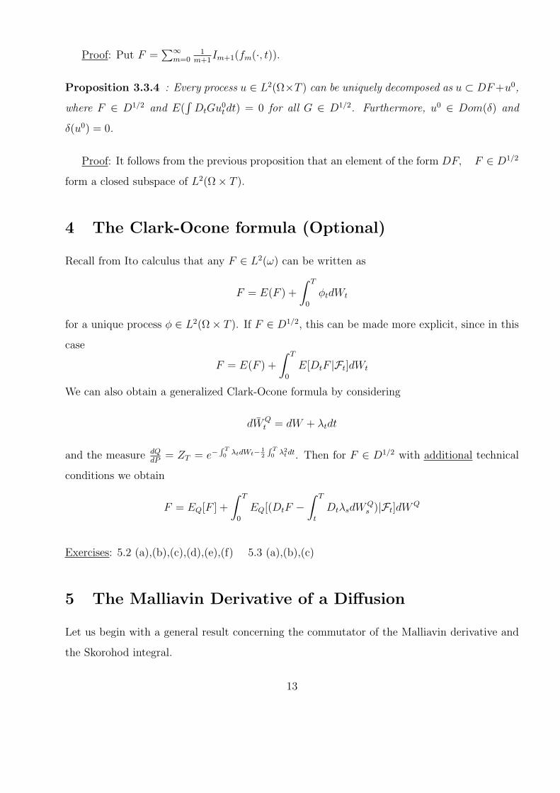
Proposition 3.3.4 : Every process u ∈ L2(Ω×T ) can be uniquely decomposed as u ⊂ DF +u0,

where F ∈ D1/2 and E(∫

DtGu0t dt) = 0 for all G ∈ D1/2. Furthermore, u0 ∈ Dom(δ) and

δ(u0) = 0.

Proof: It follows from the previous proposition that an element of the form DF, F ∈ D1/2

form a closed subspace of L2(Ω× T ).

4 The Clark-Ocone formula (Optional)

Recall from Ito calculus that any F ∈ L2(ω) can be written as

F = E(F ) +

∫ T

0

φtdWt

for a unique process φ ∈ L2(Ω× T ). If F ∈ D1/2, this can be made more explicit, since in this

case

F = E(F ) +

∫ T

0

E[DtF |Ft]dWt

We can also obtain a generalized Clark-Ocone formula by considering

dWQt = dW + λtdt

and the measure dQdP

= ZT = e−R T0 λtdWt− 1

2

R T0 λ2

t dt. Then for F ∈ D1/2 with additional technical

conditions we obtain

F = EQ[F ] +

∫ T

0

EQ[(DtF −∫ T

t

DtλsdWQs )|Ft]dWQ

Exercises: 5.2 (a),(b),(c),(d),(e),(f) 5.3 (a),(b),(c)

5 The Malliavin Derivative of a Diffusion

Let us begin with a general result concerning the commutator of the Malliavin derivative and

the Skorohod integral.

13

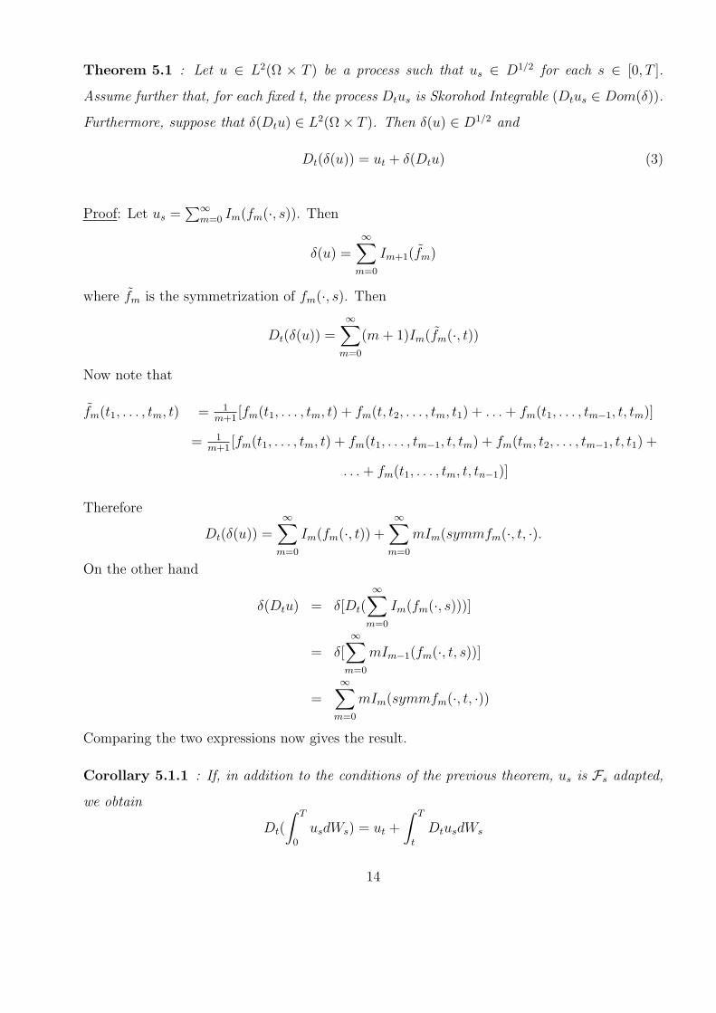
Theorem 5.1 : Let u ∈ L2(Ω × T ) be a process such that us ∈ D1/2 for each s ∈ [0, T ].

Assume further that, for each fixed t, the process Dtus is Skorohod Integrable (Dtus ∈ Dom(δ)).

Furthermore, suppose that δ(Dtu) ∈ L2(Ω× T ). Then δ(u) ∈ D1/2 and

Dt(δ(u)) = ut + δ(Dtu) (3)

Proof: Let us =∑∞

m=0 Im(fm(·, s)). Then

δ(u) =∞∑

m=0

Im+1(fm)

where fm is the symmetrization of fm(·, s). Then

Dt(δ(u)) =∞∑

m=0

(m + 1)Im(fm(·, t))

Now note that

fm(t1, . . . , tm, t) = 1m+1

[fm(t1, . . . , tm, t) + fm(t, t2, . . . , tm, t1) + . . . + fm(t1, . . . , tm−1, t, tm)]

= 1m+1

[fm(t1, . . . , tm, t) + fm(t1, . . . , tm−1, t, tm) + fm(tm, t2, . . . , tm−1, t, t1) +

. . . + fm(t1, . . . , tm, t, tn−1)]

Therefore

Dt(δ(u)) =∞∑

m=0

Im(fm(·, t)) +∞∑

m=0

mIm(symmfm(·, t, ·).

On the other hand

δ(Dtu) = δ[Dt(∞∑

m=0

Im(fm(·, s)))]

= δ[∞∑

m=0

mIm−1(fm(·, t, s))]

=∞∑

m=0

mIm(symmfm(·, t, ·))

Comparing the two expressions now gives the result.

Corollary 5.1.1 : If, in addition to the conditions of the previous theorem, us is Fs adapted,

we obtain

Dt(

∫ T

0

usdWs) = ut +

∫ T

t

DtusdWs

14

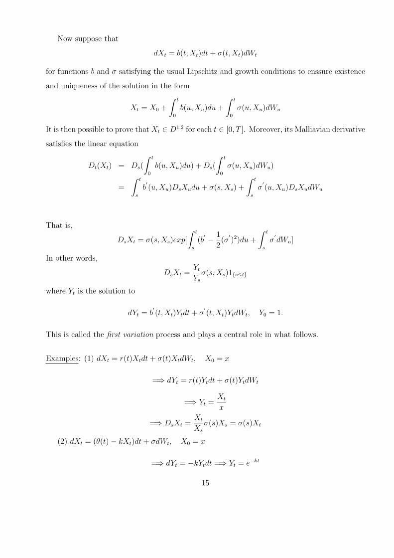
Now suppose that

dXt = b(t,Xt)dt + σ(t,Xt)dWt

for functions b and σ satisfying the usual Lipschitz and growth conditions to enssure existence

and uniqueness of the solution in the form

Xt = X0 +

∫ t

0

b(u, Xu)du +

∫ t

0

σ(u, Xu)dWu

It is then possible to prove that Xt ∈ D1,2 for each t ∈ [0, T ]. Moreover, its Malliavian derivative

satisfies the linear equation

Dt(Xt) = Ds(

∫ t

0

b(u, Xu)du) + Ds(

∫ t

0

σ(u, Xu)dWu)

=

∫ t

s

b′(u, Xu)DsXudu + σ(s, Xs) +

∫ t

s

σ′(u, Xu)DsXudWu

That is,

DsXt = σ(s, Xs)exp[

∫ t

s

(b′ − 1

2(σ

′)2)du +

∫ t

s

σ′dWu]

In other words,

DsXt =Yt

Ys

σ(s, Xs)1s≤t

where Yt is the solution to

dYt = b′(t,Xt)Ytdt + σ

′(t,Xt)YtdWt, Y0 = 1.

This is called the first variation process and plays a central role in what follows.

Examples: (1) dXt = r(t)Xtdt + σ(t)XtdWt, X0 = x

=⇒ dYt = r(t)Ytdt + σ(t)YtdWt

=⇒ Yt =Xt

x

=⇒ DsXt =Xt

Xs

σ(s)Xs = σ(s)Xt

(2) dXt = (θ(t)− kXt)dt + σdWt, X0 = x

=⇒ dYt = −kYtdt =⇒ Yt = e−kt

15

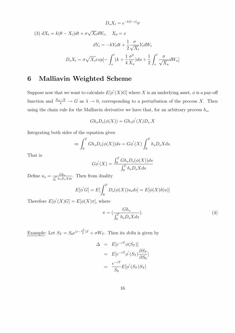
DsXt = e−k(t−s)σ

(3) dXt = k(θ −Xt)dt + σ√

XtdWt, X0 = x

dYt = −kYtdt +1

2

σ√Xt

YtdWt

DsXt = σ√

Xsexp[−∫ t

s

(k +1

4

σ2

Xu

)du +1

2

∫ t

s

σ√Xu

dWu]

6 Malliavin Weighted Scheme

Suppose now that we want to calculate E[φ′(X)G] where X is an underlying asset, φ is a pay-off

function and Xλ−Xλ

→ G as λ → 0, corresponding to a perturbation of the process X. Then

using the chain rule for the Malliavin derivative we have that, for an arbitrary process hs,

GhsDs(φ(X)) = Ghsφ′(X)Ds.X

Integrating both sides of the equation gives

⇒∫ T

0

GhsDs(φ(X))ds = Gφ′(X)

∫ T

0

hsDsXds.

That is

Gφ′(X) =

∫ T

0GhsDs(φ(X))ds∫ T

0hsDsXds

Define us = GhsR T0 hsDsXds

. Then from duality

E[φ′G] = E[

∫ T

0

Ds(φ(X))usds] = E[φ(X)δ(u)]

Therefore E[φ′(X)G] = E[φ(X)π], where

π = (Ghs∫ T

0hsDsXds

). (4)

Example: Let ST = S0e(r−σ2

2)T + σWT . Then its delta is given by

∆ = E[e−rT φ(ST )]

= E[e−rT φ′(ST )

∂ST

∂S0

]

=e−rT

S0

E[φ′(ST )ST ]

16

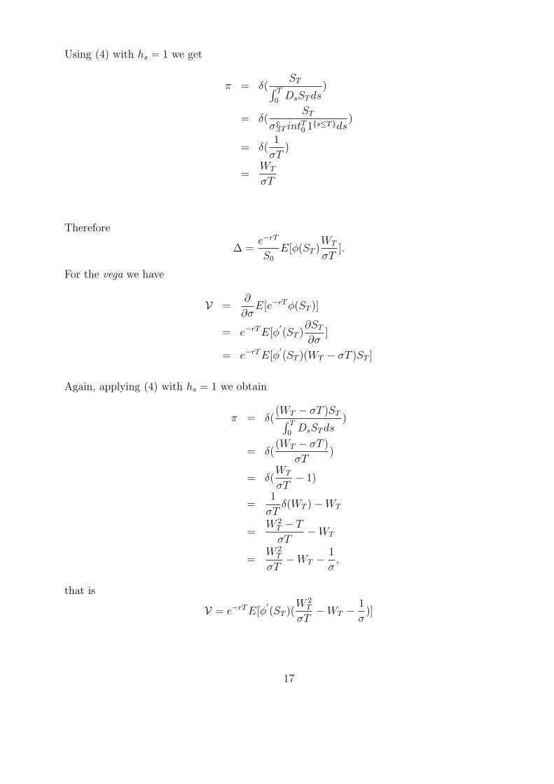
Using (4) with hs = 1 we get

π = δ(ST∫ T

0DsST ds

)

= δ(ST

σ§T intT0 1s≤Tds)

= δ(1

σT)

=WT

σT

Therefore

∆ =e−rT

S0

E[φ(ST )WT

σT].

For the vega we have

V =∂

∂σE[e−rT φ(ST )]

= e−rT E[φ′(ST )

∂ST

∂σ]

= e−rT E[φ′(ST )(WT − σT )ST ]

Again, applying (4) with hs = 1 we obtain

π = δ((WT − σT )ST∫ T

0DsST ds

)

= δ((WT − σT )

σT)

= δ(WT

σT− 1)

=1

σTδ(WT )−WT

=W 2

T − T

σT−WT

=W 2

T

σT−WT −

1

σ,

that is

V = e−rT E[φ′(ST )(

W 2T

σT−WT −

1

σ)]

17

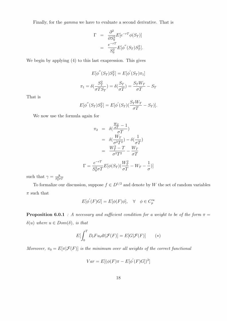
Finally, for the gamma we have to evaluate a second derivative. That is

Γ =∂2

∂S20

E[e−rT φ(ST )]

=e−rT

S20

E[φ′′(ST )S2

T ].

We begin by applying (4) to this last exapression. This gives

E[φ′′(ST )S2

T ] = E[φ′(ST )π1]

π1 = δ(S2

T

σTST

) = δ(ST

σT) =

ST WT

σT− ST

That is

E[φ′′(ST )S2

T ] = E[φ′(ST )(

ST WT

σT− ST )].

We now use the formula again for

π2 = δ(WT

σT− 1

σT)

= δ(WT

σ2T 2)− δ(

1

σT)

=W 2

T − T

σ2T 2− WT

σT

Γ =e−rT

S20σT

E[φ(ST )(W 2

T

σT−WT −

1

σ)]

such that γ = vS2

0σT

To formalize our discussion, suppose f ∈ D1/2 and denote by W the set of random variables

π such that

E[φ′(F )G] = E[φ(F )φ], ∀ φ ∈ C∞

p

Proposition 6.0.1 : A necessary and sufficient condition for a weight to be of the form π =

δ(u) where u ∈ Dom(δ), is that

E[

∫ T

0

DtFutdt|F(F )] = E[G|F(F )] (∗)

Moreover, π0 = E[π|F(F )] is the minimum over all weights of the correct functional

V ar = E[(φ(F )π − E[φ′(F )G])2]

18

Proof: Suppose that u ∈ Dom(δ) satisfies

E[

∫ T

0

DtFutdt|σ(F )] = E[G|σ(F )]

Then

E[φ′(F )G] = E[E[φ

′(F )G|σ(F )]]

= E[φ′(F )E[G|σ(F )]]

= E[φ′(F )E[

∫ T

0

DtFutdt|σ(F )]]

= E[

∫ T

0

Dtφ(F )utdt]

= E[φ(F )δ(u)dt]

so π = δ(u) is a weight.

Conversely, if π = δ(u) for some u ∈ Dom(δ) is a weight, then

E[φ′(F )G] = E[φδ(u)]

= E[

∫ T

0

Dtφ(F )utdt]

= E[φ′(F )

∫ T

0

DtFutdt]

Therefore,

E[

∫ T

0

DtFutdt|σ(F )] = E[G|σ(F )].

To prove the minimal variance claim, observe first that for any two weights π1, π2 we must

have E[π1|σ(F )] = E[π2|σ(F )]. Therefore, setting π0 = E[π|σ(F )] for a generic weight π we

obtain

varπ = E[(φ(F )π − E[φ′(F )G])2]

= E[(φ(F )(π − π0) + φ(F )π0 − E[φ′(F )G])2]

= E[(φ(F )(π − π0))2] + E[(φ(F )π0 − E[φ

′(F )G])2]

+ 2E[φ(F )(π − π0)(φ(F )π0 − E[φ′(F )G])]

19

But

E[φ(F )(π − π0)(φ(F )π0 − E[φ′(F )G])] = E[E[φ(F )(π − π0)(φ(F )π0 − E[φ

′(F )G])]|σ(F )] = 0.

Therefore the minimum must be achieved for π = π0.

7 Generalized Greeks

Consider now

dXt = r(t)Xtdt + σ(t,Xt)dWt, X0 = x

where r(t) is a deterministic function and σ(·, ·) satisfies the Lipschitz, boundedness and uniform

ellipticity condition. Let r(t), σ(·, ·) be two directions such that (r + εrt) and (σ + εσ) satisfy

the same conditions for any ε ∈ [−1, 1].

Define

dXε1t = (r(t) + ε1r)X

ε1t + σ(t,Xε1

t )dWt

dXε2t = r(t)Xε2

t + [σ(t,Xε2t ) + ε2σ(t,Xε2

t )]dWt

Consider also the price functionals, for a square integral pay-off function of the form φ : Rm →

R.

P (x) = EQx [e−

R T0 r(t)dtφ(Xt1 , . . . , Xtm)]

P ε1(x) = EQx [e−

R T0 (r(t)+ε1r(t))dtφ(Xε1

t1 , . . . , Xε1tm)]

P ε2(x) = EQx [e−

R T0 r(t)dtφ(Xε2

t1 , . . . , Xε2tm)]

Then the generalized Greeks are defined as

∆ =∂P (x)

∂x, Γ =

∂2P

∂x2

ρ =∂P ε1

∂ε1

|ε1=0,r, V =∂P ε2

∂ε2

|ε2=0,σ

The next proposition shows that the variations with respect to both the drift and the

diffusion coefficients for the process Xt can be expressed in terms of the first variation process

Yt defined previously.

Proposition 7.0.2 : The following limits hold in L2–convergence

20

1. limε1→0X

ε1t −Xt

ε1=

∫ t

0Ytr(s)Xs

Ysds

2. limε2→0X

ε2t −Xt

ε2=

∫ t

0Yt

σ(s,Xs)Ys

dWs −∫ t

0Yt

σ′(s,Xs)σ(s,Xs)

Ysds

8 General One–Dimensional Diffusions

Now we return to the general diffusion SDE

dXt = b(t,Xt)dt + σ(t,Xt)dWt

where the deterministic functions b, σ satisfy the usual conditions for existence and uniqueness.

We will find several ways to specify Malliavin weights for delta: similar formulas can be found

for the other greeks. An important point not addressed in these notes is to understand the

computational issues when using Monte Carlo simulation. This will involve the practical prob-

lem of knowing which processes in addition to Xt itself need to be sampled to compute the

weight: the answer in general is to compute the variation processes Yt, Y(2)t , Y

(3)t , . . . .

Recall the conditions for π = δ(wt) to be a weight for delta:

E[

∫ T

0

σt

Yt0

wtdt|σ(Xti)] = E[YT0|σ(Xti)]

Our solutions will solve the stronger, sufficient conditions:∫ T

0

σt

Yt0

wtdt = YT0

We investigate in more detail two special forms for w. We will see the need from this to

look at higher order Malliavin derivatives: the calculus for this is given in the final section.

1. We obtain a t independent weight analogous to the construction in Ben-hamou (2001) by

letting

wt = wT =

[∫ T

0

σt

Yt0

dt

]−1

To compute δ(w) use (1) to give δ(w) = wWT −∫ T

0Dtwdt. From the quotient rule

Dt(A−1) = −A−1DtA A−1 and the commutation relation (3) we obtain

Dtw = −w2Y −1t0

∫ T

t

[DtσsYst − σsDtYst

Y 2st

]ds (5)

= −w2Y −1t0

∫ T

t

[DtσsYst − σsDtYst

Y 2st

]ds (6)

(7)

21

where we use the general formula for DtYst derived in the next section. This yields the

final formula

π = −∫ T

0

∫ T

t

w2Y −1t0

[σ′sσt − Yst − σsDtYst

Y 2st

]ds dt

Computing this weight will be computationally intensive: in addition to sampling Xt, one

needs Yt, Y(2)t .

2. We obtain a t dependent weight analogous to the construction in Ben-hamou (2001) by

letting

wt =Yt0

Tσt

. This yields the weight as an ordinary Ito integral:

π =

∫ T

0

Yt0

Tσt

dWt

Numerical simulation of Xt, Yt will be sufficient to compute this weight.

.

9 Higher Order Malliavin Derivatives

In this section, we sketch out the properties of the higher order variation processes

Y(k)st =

∂kXs

∂Xkt

, t < s

and use them to compute multiple Malliavin derivatives Dt1 . . . DtkXs. These formulas are

usually necessary for higher order greeks like γ. But as seen in the previous section it may also

enter formulas for delta when certain weights are chosen.

Here are the SDEs satisfied by the first three variation processes:

dYt = b′tYtdt + σ′tYtdWt (8)

dY(2)t =

[b′tY

(2)t + b′′t Y

2t

]dt +

[σ′tY

(2)t + σ′′t Y

2t

]dWt (9)

dY(3)t =

[b′tY

(3)t + 3b′′t YtY

(2)t + b′′′t Y 3

t

]dt +

[σ′tY

(3)t + 3σ′′t YtY

(2)t + σ′′′t Y 3

t

]dWt (10)

(11)

22

One can see that the pattern is

dY(k)t = b′tY

(k)t dt + σ′tY

(k)t dWt + F

(k)t dt + G

(k)t dWt

where F (k), G(k)t are explicit functions of t,X, (Y (j))j<k. This particular form of SDE can be

integrated by use of the semigroup defined by Yts.

Proposition 9.0.3

Yk)t = Yt0

∫ t

0

Y −1u0

[(F (k)

u −G(k)u σu)du + G(k)

u dWu

]Proof: From the product rule dXY = dX(Y + dY ) + XdY for stochastic processes

d(RHS) = [b′tYt0dt + σ′tYt0dWt][Y −1

t0 Y(k)t + Y −1

t0 (F(k)t −G

(k)t σ′t)dt + G

(k)t dWt

]+Yt0

[Y −1

t0 (F(k)t −G

(k)t σ′t)dt + G

(k)t dWt

]= b′tY

(k)t + σ′tY

(k)t dWt + G

(k)t σ′tdt + (F

(k)t −G

(k)t σ′)dt + G

(k)t dWt

= d(LHS)

ut

Since the higher variation processes have the interpretation of higher derivatives of X with

respect to the initial value x, we can extend the notion to derivatives with respect to Xt, any

t. For that we define

Y(k)t0 =

Y(k)t

Yt0

and then note

Y(k)s0 − Y

(k)t0 =

∫ s

t

Y −1u0

[(F (k)

u −G(k)u σu)du + G(k)

u dWu

]If we define

Y(k)st := Yt0[Y

(k)s0 − Y

(k)t0 ]

then Y(k)st solves (9.0.3) for s > t, subject to the initial condition Y

(k)tt = 0. Therefore Y

(k)st has

the interpretation of ∂kXs

∂Xkt

.

The following rules extend the Malliavin calculus to higher order derivatives:

1. Chain rule:

DtF (Xs) = F ′(Xs)DtXs, t < s;

23

2.∂Xs

∂Xt

:= YstI(t < s) := Y(1)st I(t < s);

3.∂Y

(k)st

∂Xt

= Y(k+1)st :=

∂k+1Xs

∂Xk+1t

, t < s;

4.

Y(k)st = Y −1

st Y(k)t0 − Y

(k)s0 ;

5.

DtXt = σt.

Examples:

1.

DtXT =∂XT

∂Xt

DtXt by chain rule

= YTtσt by (2), (5)

2.

DtYs0 = (DtYst)Yt0 = Y(2)st (DtXt)Yt0

3. For t < s < T :

Dt[DsXT ] =∂

∂Xs

[YTsσsI(s < T )] DtXs by chain rule

=[Y

(2)Ts σt + YTsσ

′s

]Ystσt

4. For t < s < T :

Ds[DtXT ] = Ds[YTsYstσt] = Y(2)Ts σsYstσt (12)

24