Many-body physics 1: Basics

Hongki Min

hmin@snu.ac.kr

Department of Physics and Astronomy, Seoul National University, Korea

Orientation, March 9, 2015

− 다체계 물리: 기본

Syllabus

Syllabus

References

[1] Condensed matter field theory

Alexander Altland and Ben Simons

[2] Many-particle physics (3rd Ed.)

Gerald D. Mahan

[3] Quantum theory of the electron liquid

Gabriele Giuliani and Giovanni Vignale

[4] Introduction to Many Body Physics

Piers Coleman

References

[5] Quantum theory of many-particle systems

Alexander L. Fetter and John Dirk Walecka

[6] A guide to Feynman diagrams in

the many-body problem, Richard D. Mattuck

[7] Quantum many-particle systems

John W. Negele and Henri Orland

[8] Quantum field theory in condensed

matter physics, Naoto Nagaosa

Special topics [1] Renormalization-group approach to interacting

fermions, R. Shankar, Rev. Mod. Phys. 66, 129 (1994)

[2] Lectures on phase transitions and

the renormalization group, Nigel Goldenfeld

[3] Introduction to superconductivity

Michael Tinkham

[4] Superconductivity, superfluids, and condensates

James F. Annett

[5] The Quantum Hall effect

Daijiro Yoshioka

Special topics [6] Interacting electrons and quantum magnetism

Assa Auerbach

[7] Quantum phase transitions

Subir Sachdev

[8] Quantum physics in one dimension

Thierry Giamarchi

[9] Geometry, topology, and physics

Mikio Nakahara

[10] The geometric phase in quantum systems

Bohm, Mostafazadeh, Koizumi, Niu, and Zwanziger

Motivation

Section

References

Mattuck, Ch.0 and Ch.1

Altland and Simons, Ch.1.1

Many-body problem

System of interacting electrons and ions

• Electron Hamiltonian

ji jii

iel

e

mH

rr

22

2

2

1

2

ionionelel HHHH

• Electron-ion interaction

Ii Ii

Iionel

eZH

,

2

Rr

• Ion Hamiltonian

JI JI

JI

I

I

I

ion

eZZ

MH

RR

22

2

2

1

2

Statistics, symmetries, effective low-energy theories

See Altland

and Simons, Ch.1

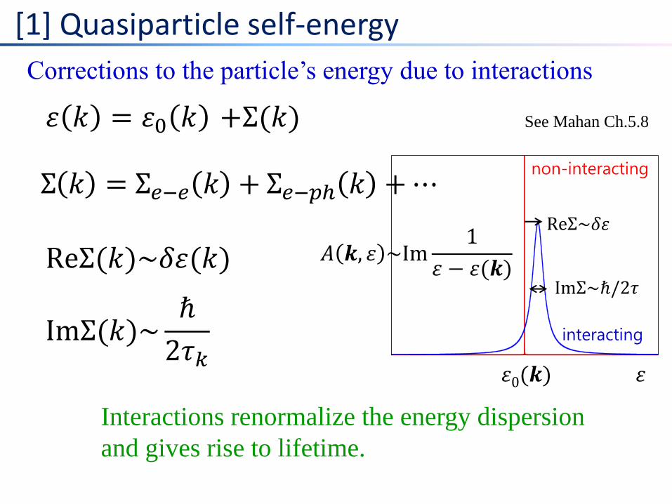
[1] Quasiparticle self-energy

휀 𝑘 = 휀0 𝑘

Corrections to the particle’s energy due to interactions

휀 휀0(𝒌)

non-interacting

𝐴 𝒌, 휀 ~Im1

휀 − 휀(𝒌)

See Mahan Ch.5.8

𝐴 𝒌, 휀 ~Im1

휀 − 휀(𝒌)

휀 휀0(𝒌)

non-interacting

ReΣ~𝛿휀

ImΣ~ℏ/2𝜏

[1] Quasiparticle self-energy

Interactions renormalize the energy dispersion

and gives rise to lifetime.

ReΣ(𝑘)~𝛿휀(𝑘)

ImΣ(𝑘)~ℏ

2𝜏𝑘

휀 𝑘 = 휀0 𝑘

Σ 𝑘 = Σ𝑒−𝑒 𝑘 + Σ𝑒−𝑝ℎ 𝑘 +⋯

Corrections to the particle’s energy due to interactions

+Σ(𝑘)

interacting

See Mahan Ch.5.8

[2] Response function

ext~ Vn n

Linking measurements to correlations

nnn ~

ext~ EJ JJ ~

ext~ HM M MMM ~

Response to the experimental probes can be expressed

in terms of correlation functions, which contain

information of the unperturbed system.

See Giuliani and Vignale, Ch.3~5

Second quantization

Section

References

Fetter & Walechka, Ch.1

Giuliani and Vignale, Ch.1.4

Occupation number representation

Identical particles and indistinguishability

𝑛𝜆1 = 1, 𝑛𝜆2 = 1

[𝑃12, 𝐻] = 0, 𝑃122 = 1

⇒ 𝑃12 = ±1 Boson/Fermion

𝜆1𝜆2 ± =1

2 𝜆1 1 𝜆2 2 ± 𝜆2 1 𝜆1 2

Example: Two identical particles

𝑛𝜆1 , 𝑛𝜆2 , 𝑛𝜆3 , … In general, Occupation number

representation

𝑃12 𝜆 1 𝜆′ 2 = 𝜆′ 1 𝜆 2

Many-body operators

𝑉 =1

2 𝑣 𝑖𝑗𝑖,𝑗

→1

2 𝑎

𝜆1′† 𝑎

𝜆2′† 𝑣𝜆1′ 𝜆2′ 𝜆1𝜆2𝑎 𝜆2𝑎 𝜆1

𝜆,𝜆′

𝐹 = 𝑓 𝑖𝑖

𝑓𝜆′𝜆= 𝜆′ 𝑓 𝜆

𝑣𝜆1′ 𝜆2′ 𝜆1𝜆2= 𝜆1′ 𝜆2

′ 𝑣 𝜆1𝜆2

Operators in the occupation number representation

One-body operators: Density, current, …

Two-body operators: Coulomb interaction, …

→ 𝑎 𝜆′† 𝑓𝜆′𝜆𝑎 𝜆

𝜆,𝜆′

See Giuliani and Vignale, App.2

Linear response theory

Section

References

Giuliani and Vignale, Ch.3~5

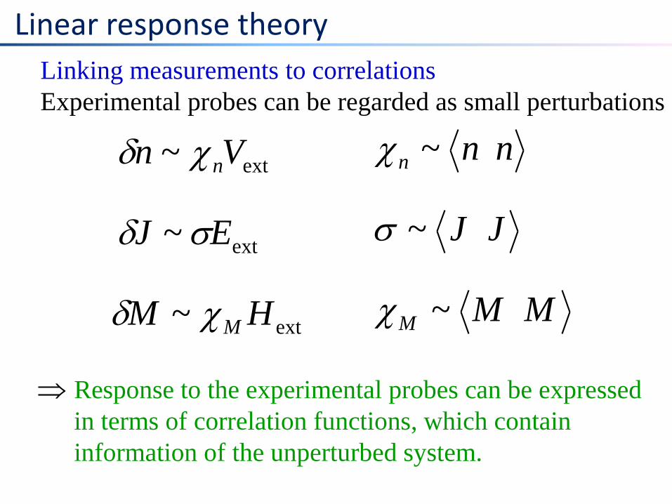
Linear response theory

ext~ Vn n

Linking measurements to correlations

Experimental probes can be regarded as small perturbations

nnn ~

ext~ EJ JJ ~

ext~ HM M MMM ~

Response to the experimental probes can be expressed

in terms of correlation functions, which contain

information of the unperturbed system.

Linear response theory

)(ˆˆ)(ˆext0 tHHtH

Linear response to an external perturbation

Response function : Retarded correlation function

)()(ˆ)(ˆext tFtBtH

)(ˆ),(ˆ)()( tBtAtttti AB

)(ˆ)(ˆ)(ˆ)(ˆext

tUtAtUtA

)(ˆ),(ˆ)(ˆext tHtAtd

itA

t

)()()(ˆ

tFtttdtA AB

𝑒𝑥 ≈ 1 + 𝑥 for 𝑥 ≪ 1

See Giuliani and

Vignale, Ch.3.2

)(ˆ1)(ˆext tHtd

itU

t

Linear response theory

Response function in frequency space

ti

mn

titi mnnm eAenAmentAm

ˆ)(ˆ

)()( tedt AB

ti

AB

)(ˆ),(ˆ)()( tBtAtttti AB

nm

nmmn

nm

nmAB BA

i

PP

, 0)(

Pn: Occupation probability for state n

Non-interacting response function

Density response of non-interacting electrons

k

k+q

𝑛𝒌 Fermi distribution function for k

𝑔 spin/valley degeneracy factor

𝑠 band index

00 )0,0( Nq

N0: DOS at EF

𝜒0 𝑞, 𝜔 = 𝑔 ∫𝑑2𝑘

2𝜋 2𝑠,𝑠′

𝑛𝒌,𝑠 − 𝑛𝒌+𝒒,𝑠′

ℏ𝜔 + 휀𝒌,𝑠 − 휀𝒌+𝒒,𝑠′ + 𝑖0+

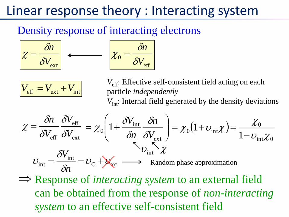
Linear response theory : Interacting system

extV

n

eff

0V

n

intexteff VVV

ext

eff

eff V

V

V

n

Density response of interacting electrons

Response of interacting system to an external field

can be obtained from the response of non-interacting

system to an effective self-consistent field

Veff: Effective self-consistent field acting on each

particle independently

Vint: Internal field generated by the density deviations

0int

0int0

11

int

ext

int0 1

V

n

n

V

xcCint

int

n

VRandom phase approximation

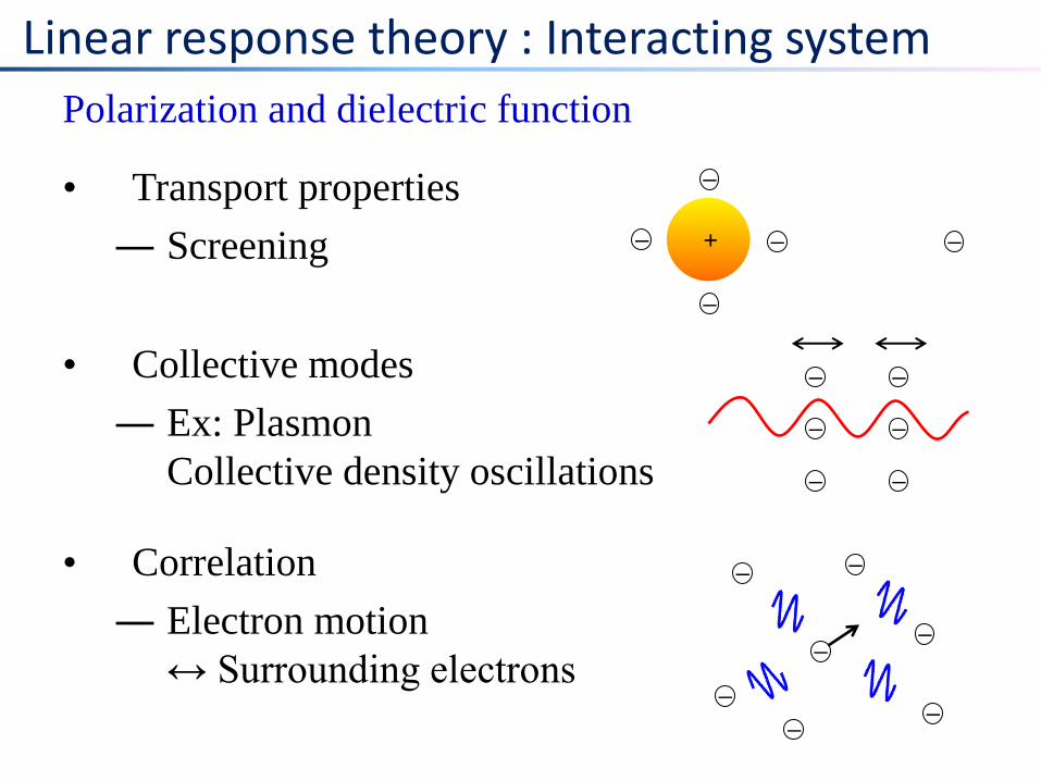
Polarization and dielectric function

Linear response theory : Interacting system

• Transport properties

― Screening

• Collective modes

― Ex: Plasmon

Collective density oscillations

• Correlation

― Electron motion

↔ Surrounding electrons

+ –

–

–

–

–

–

–

–

–

–

–

–

–

–

–

–

–

–

Green’s function

Section

References

Fetter & Walechka, Ch.3 and Ch.7

Mahan, Ch.2 and Ch.3

Single particle Green’s function (I)

𝑖𝐺 𝑘, 𝑡 = Ω 𝑇𝑐 𝐻𝑘 𝑡 𝑐 𝐻𝑘† (0) Ω

𝑇𝐴 𝑡 𝐵(𝑡′) 𝐴 𝑡 𝐵(𝑡′) 𝑡 > 𝑡′

±𝐵(𝑡′)𝐴 𝑡 𝑡′ > 𝑡

𝑇: Time-ordering operator

𝐻: Heisenberg picture

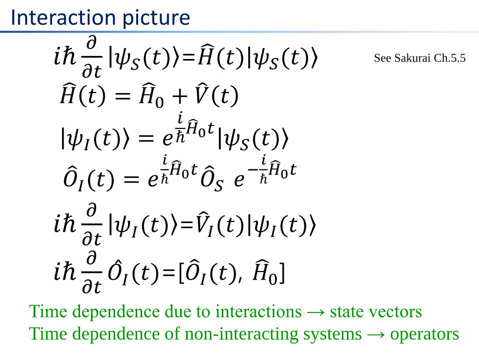
Interaction picture

𝑖ℏ𝜕

𝜕𝑡 𝜓𝑆(𝑡) =𝐻 (𝑡) 𝜓𝑆(𝑡)

𝐻 𝑡 = 𝐻 0 + 𝑉 𝑡

𝜓𝐼(𝑡) = 𝑒𝑖ℏ𝐻 0𝑡 𝜓𝑆(𝑡)

See Sakurai Ch.5.5

𝑂 𝐼(𝑡) = 𝑒𝑖

ℏ𝐻 0𝑡𝑂 𝑆 𝑒

−𝑖

ℏ𝐻 0𝑡

𝑖ℏ𝜕

𝜕𝑡 𝜓𝐼(𝑡) =𝑉 𝐼(𝑡) 𝜓𝐼(𝑡)

𝑖ℏ𝜕

𝜕𝑡𝑂 𝐼(𝑡)=[𝑂 𝐼(𝑡), 𝐻 0]

Time dependence due to interactions → state vectors

Time dependence of non-interacting systems → operators

Single particle Green’s function (II)

𝑖𝐺 𝑘, 𝑡 = Ω 𝑇𝑐 𝐻𝑘 𝑡 𝑐 𝐻𝑘† (0) Ω

=0 𝑇𝑐 𝑘 𝑡 𝑐 𝑘

†0 𝑈 𝐼(∞,−∞) 0

0 𝑈 𝐼(∞,−∞) 0

= 0 𝑇𝑐 𝑘 𝑡 𝑐 𝑘† 0 𝑈 𝐼 ∞,−∞ 0

𝑐𝑜𝑛𝑛

Interaction

picture

Connected

diagrams

Linked cluster theorem; Wick’s theorem;

Perturbation theory; Feynman diagrams; Self-energy

See Mahan Ch.2 and

Fetter and Walecka, Ch.3

𝑈 𝐼 𝑡, 𝑡0 = 𝑇exp −𝑖

ℏ 𝑑𝑡′𝑡

𝑡0

𝑉𝐼(𝑡′)

Single particle Green’s function (II)

Corrections to the particle’s energy due to interactions

휀 휀0(𝒌)

non-interacting

𝐴 𝒌, 휀 ~Im𝐺(𝒌, 휀)

See Mahan Ch.5.8

𝐺(0) 𝒌, 휀 =1

휀 − 휀𝒌 + 𝑖𝜂𝒌

𝐴 𝒌, 휀 ~Im𝐺(𝒌, 휀)

휀 휀0(𝒌)

non-interacting

ReΣ~𝛿휀

ImΣ~ℏ/2𝜏

Single particle Green’s function (II)

Interactions renormalize the energy dispersion

and gives rise to lifetime.

ReΣ(𝒌)~𝛿휀(𝒌)

ImΣ(𝒌)~ℏ

2𝜏𝒌

Corrections to the particle’s energy due to interactions

interacting

See Mahan Ch.5.8

𝐺 𝒌, 휀 =1

휀 − 휀𝒌 − Σ(𝒌, 휀)

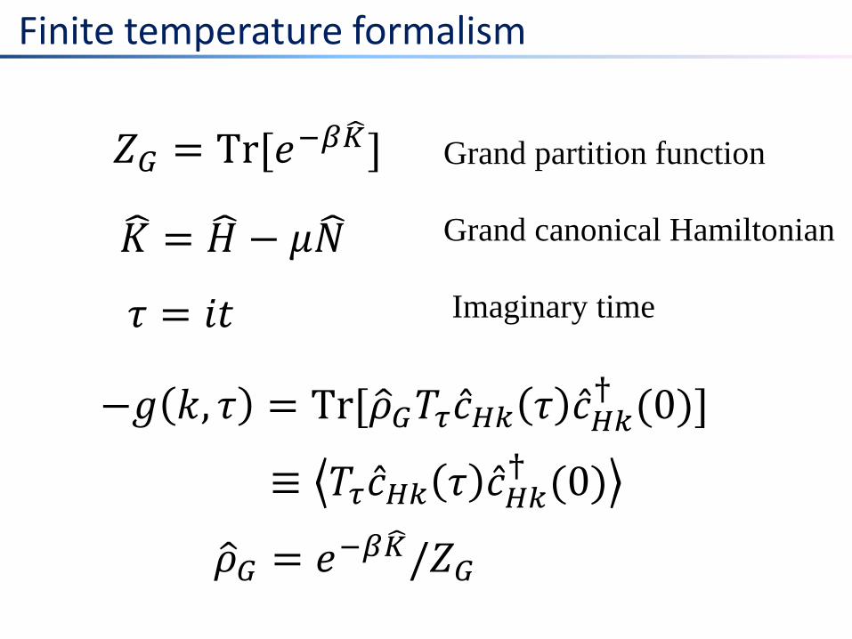
Finite temperature formalism

𝑍𝐺 = Tr[𝑒−𝛽𝐾 ]

𝐾 = 𝐻 − 𝜇𝑁

−𝑔 𝑘, 𝜏 = Tr[𝜌 𝐺𝑇𝜏𝑐 𝐻𝑘 𝜏 𝑐 𝐻𝑘† (0)]

Grand partition function

Grand canonical Hamiltonian

≡ 𝑇𝜏𝑐 𝐻𝑘 𝜏 𝑐 𝐻𝑘† (0)

𝜏 = 𝑖𝑡 Imaginary time

𝜌 𝐺 = 𝑒−𝛽𝐾 /𝑍𝐺

Analytic continuation

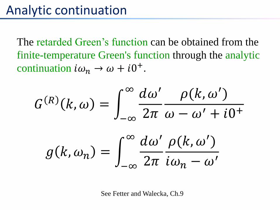
The retarded Green’s function can be obtained from the

finite-temperature Green's function through the analytic

continuation 𝑖𝜔𝑛 → 𝜔 + 𝑖0+.

See Fetter and Walecka, Ch.9

𝐺 𝑅 𝑘, 𝜔 = 𝑑𝜔′

2𝜋

∞

−∞

𝜌(𝑘, 𝜔′)

𝜔 − 𝜔′ + 𝑖0+

𝑔 𝑘,𝜔𝑛 = 𝑑𝜔′

2𝜋

∞

−∞

𝜌(𝑘, 𝜔′)

𝑖𝜔𝑛 −𝜔′

Functional integral method

Section

References

Coleman, Ch.13

Altland and Simons, Ch.4

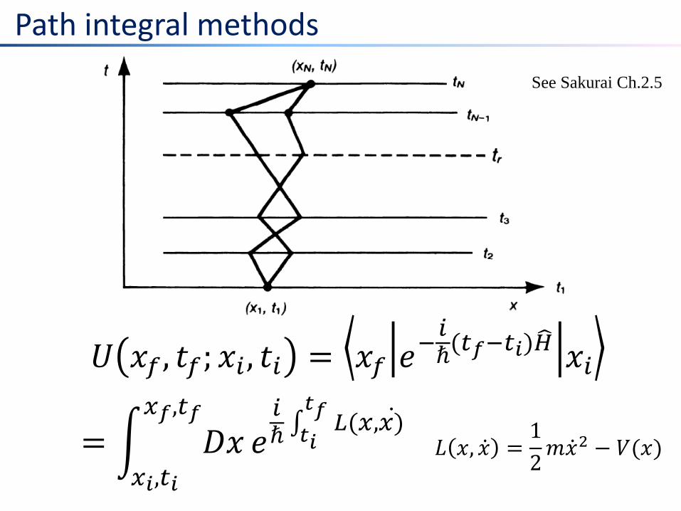
Path integral methods

See Sakurai Ch.2.5

𝑈 𝑥𝑓, 𝑡𝑓; 𝑥𝑖 , 𝑡𝑖 = 𝑥𝑓 𝑒−𝑖ℏ(𝑡𝑓−𝑡𝑖)𝐻 𝑥𝑖

= 𝐷𝑥𝑥𝑓,𝑡𝑓

𝑥𝑖,𝑡𝑖

𝑒𝑖ℏ ∫

𝐿(𝑥,𝑥) 𝑡𝑓𝑡𝑖 𝐿 𝑥, 𝑥 =

1

2𝑚𝑥 2 − 𝑉(𝑥)

Functional integral methods

𝑍𝐺 = Tr[𝑒−𝛽𝐾 ]

= 𝐷𝜙∗𝐷𝜙 𝑒−𝑆[𝜙∗,𝜙]

𝑆[𝜙∗, 𝜙] = 𝑑𝜏𝛽

0

𝜙∗𝜕

𝜕𝜏𝜙 + 𝐾(𝜙∗, 𝜙)

𝑎 𝜙 = 𝜙 𝜙 coherent states

See Negele and Orland, Ch.2.2

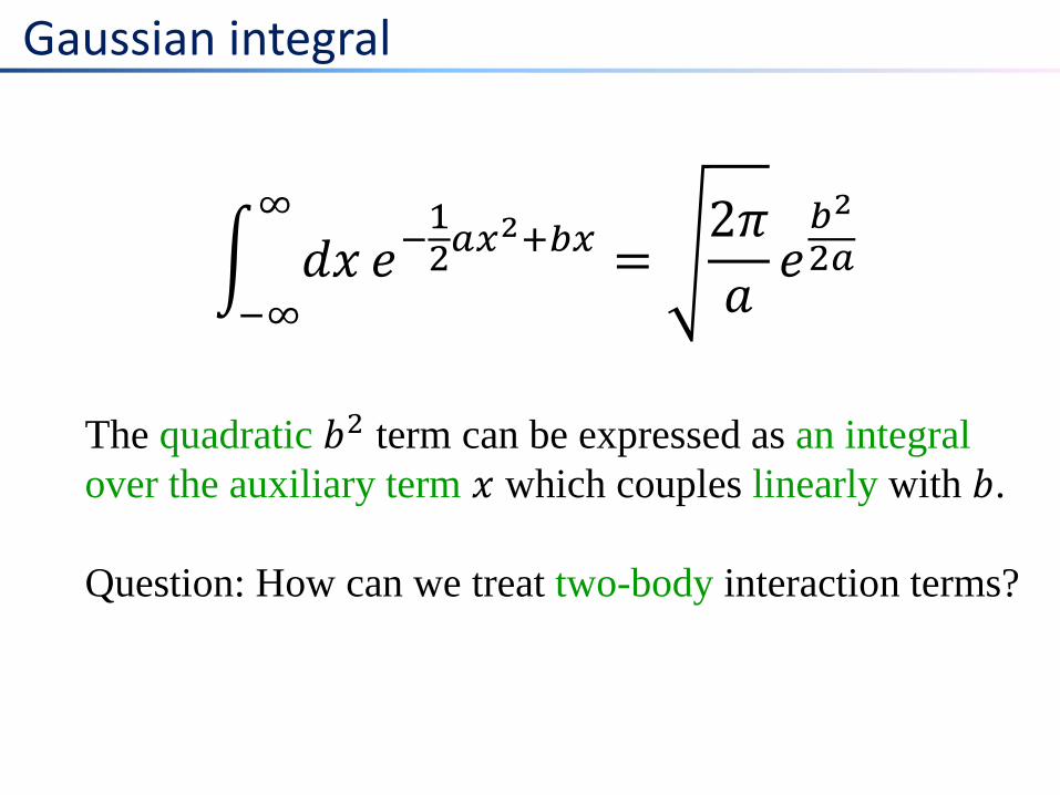
Gaussian integral

𝑑𝑥∞

−∞

𝑒−12𝑎𝑥2+𝑏𝑥 =

2𝜋

𝑎𝑒𝑏2

2𝑎

The quadratic 𝑏2 term can be expressed as an integral

over the auxiliary term 𝑥 which couples linearly with 𝑏.

Question: How can we treat two-body interaction terms?

Hubbard-Stratonovich transformation

Two-body fermionic operators can be expressed as an

integral over the auxiliary field which couples linearly

with the ferminonic operators.

This transformation represents the interactions between

fermions in terms of an exchange boson.

By integrating out the microscopic fermions, we can

rewrite the problem as an effective field theory of the

bosonic order parameter 𝜙.

See Coleman Ch.13.5

𝜌 = 𝜓 𝜓

Phase transition and broken symmetry

Section

References

Coleman, Ch.12

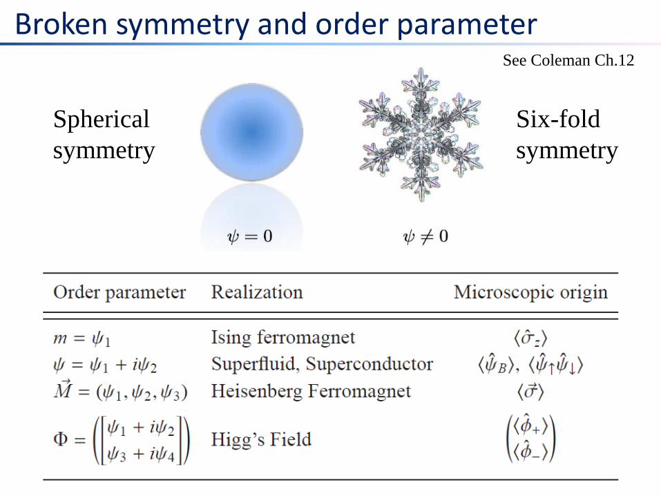
Broken symmetry and order parameter See Coleman Ch.12

Spherical

symmetry Six-fold

symmetry

Landau-Ginzburg theory

𝑓 𝜙 =1

2𝛻𝜙 2 +

𝑟

2𝜙2 +

𝑢

4𝜙4 − ℎ𝜙

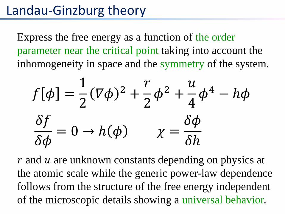
Express the free energy as a function of the order

parameter near the critical point taking into account the

inhomogeneity in space and the symmetry of the system.

𝑟 and 𝑢 are unknown constants depending on physics at

the atomic scale while the generic power-law dependence

follows from the structure of the free energy independent

of the microscopic details showing a universal behavior.

𝛿𝑓

𝛿𝜙= 0 → ℎ 𝜙 𝜒 =

𝛿𝜙

𝛿ℎ

Renormalization group

Section

References

Shankar, Sec.I

Goldenfeld, Ch.9

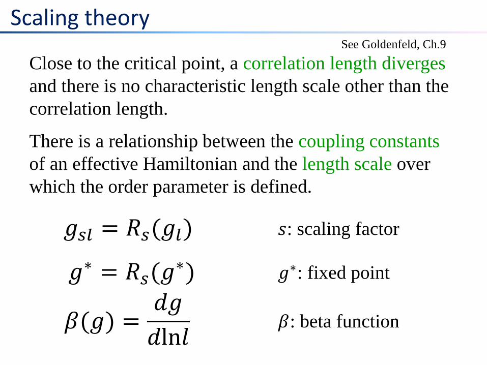
Scaling theory

Close to the critical point, a correlation length diverges

and there is no characteristic length scale other than the

correlation length.

There is a relationship between the coupling constants

of an effective Hamiltonian and the length scale over

which the order parameter is defined.

𝑔𝑠𝑙 = 𝑅𝑠(𝑔𝑙) 𝑠: scaling factor

𝛽(𝑔) =𝑑𝑔

𝑑ln𝑙 𝛽: beta function

𝑔∗ = 𝑅𝑠(𝑔∗) 𝑔∗: fixed point

See Goldenfeld, Ch.9

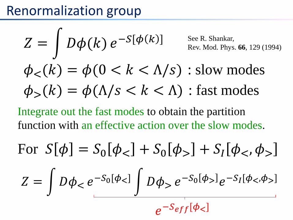
𝑍 = 𝐷𝜙< 𝑒−𝑆0[𝜙<] 𝐷𝜙> 𝑒

−𝑆0 𝜙> 𝑒−𝑆𝐼[𝜙<,𝜙>]

Renormalization group

See R. Shankar,

Rev. Mod. Phys. 66, 129 (1994) 𝑍 = 𝐷𝜙(𝑘) 𝑒−𝑆[𝜙 𝑘 ]

𝜙<(𝑘) = 𝜙(0 < 𝑘 < Λ/𝑠) : slow modes

𝜙>(𝑘) = 𝜙(Λ/𝑠 < 𝑘 < Λ) : fast modes

Integrate out the fast modes to obtain the partition

function with an effective action over the slow modes.

For 𝑆 𝜙 = 𝑆0 𝜙< + 𝑆0 𝜙> + 𝑆𝐼 𝜙<, 𝜙>

𝑒−𝑆𝑒𝑓𝑓[𝜙<]

φ4 theory: Effective theory of Ising spins

See Altland and Simons, Ch.8.4

𝐻 = −1

2 𝐽𝑖𝑗𝑆𝑖𝑆𝑗

𝑖,𝑗∈𝑁.𝑁.

𝑆𝑖 = ±1

𝑆 𝜙 = 1

2𝛻𝜙 2 +

𝑟

2𝜙2 +

𝑢

4𝜙4

Example: Plasmons

Section

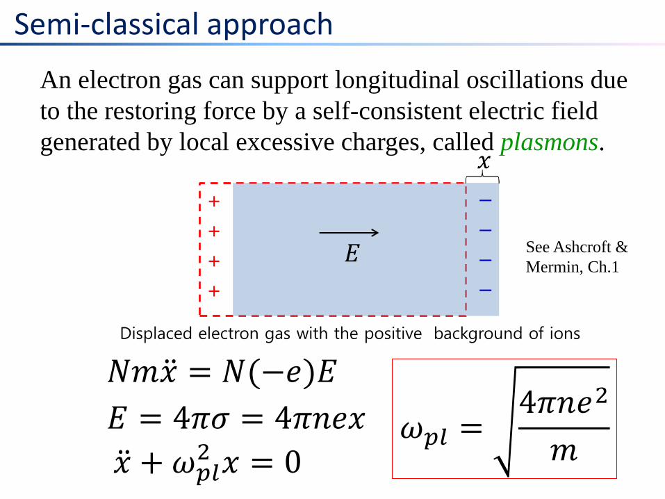
Semi-classical approach

An electron gas can support longitudinal oscillations due

to the restoring force by a self-consistent electric field

generated by local excessive charges, called plasmons.

𝑁𝑚𝑥 = 𝑁(−𝑒)𝐸

𝐸 = 4𝜋𝜎 = 4𝜋𝑛𝑒𝑥 𝜔𝑝𝑙 =4𝜋𝑛𝑒2

𝑚

See Ashcroft &

Mermin, Ch.1

𝑥 + 𝜔𝑝𝑙2 𝑥 = 0

+

+

+

+

−

−

−

−

Displaced electron gas with the positive background of ions

𝑥

𝐸

Many-body approach

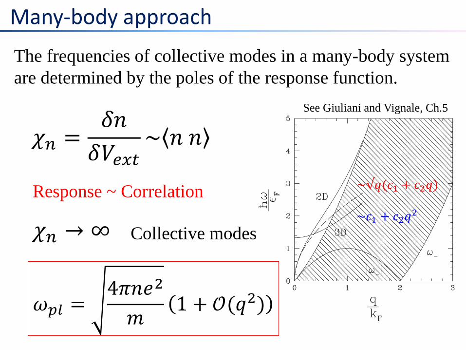
The frequencies of collective modes in a many-body system

are determined by the poles of the response function.

𝜒𝑛 =𝛿𝑛

𝛿𝑉𝑒𝑥𝑡~ 𝑛 𝑛

Response ~ Correlation

See Giuliani and Vignale, Ch.5

~√𝑞(𝑐1 + 𝑐2𝑞)

~𝑐1 + 𝑐2𝑞2

𝜔𝑝𝑙 =4𝜋𝑛𝑒2

𝑚1 + 𝒪(𝑞2)

𝜒𝑛 → ∞ Collective modes

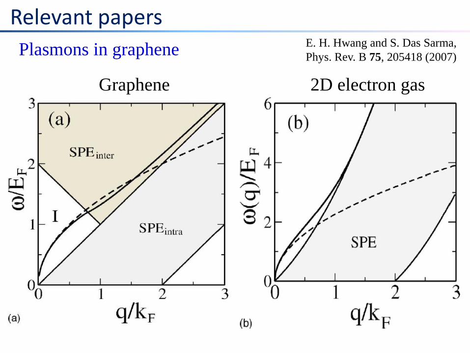
Plasmons in graphene

Relevant papers E. H. Hwang and S. Das Sarma,

Phys. Rev. B 75, 205418 (2007)

Graphene 2D electron gas