math 756 complex variables ii - information services …matveev/courses/m756_f13/conformal.pdf ·...
TRANSCRIPT
Math 756 Complex Variables II
Prof L.J. Cummings∗
November 4, 2010
Contents
1 Review of Complex I, and extensions 31.1 Elementary definitions . . . . . . . . . . . . . . . . . . . . . . 31.2 Analytic functions: The basics . . . . . . . . . . . . . . . . . . 41.3 Complex Integration . . . . . . . . . . . . . . . . . . . . . . . 91.4 Poisson’s integral formulae for solutions of Laplace’s equation 12
1.4.1 Poisson integral formula for a circle . . . . . . . . . . . 121.4.2 Poisson integral formula for a half-space . . . . . . . . 16
1.5 Taylor series, Laurent series . . . . . . . . . . . . . . . . . . . 181.6 Singular points . . . . . . . . . . . . . . . . . . . . . . . . . . 20
1.6.1 Caserati-Weierstrass Theorem . . . . . . . . . . . . . . 221.7 Analytic continuation . . . . . . . . . . . . . . . . . . . . . . . 23
1.7.1 Natural barriers . . . . . . . . . . . . . . . . . . . . . . 29
2 Cauchy’s Residue theorem (and others) and Applications 312.1 Cauchy’s Residue Theorem . . . . . . . . . . . . . . . . . . . . 31
2.1.1 Application to summing series . . . . . . . . . . . . . . 322.2 Principle of the argument & Rouche’s theorem . . . . . . . . . 342.3 Integral transform methods . . . . . . . . . . . . . . . . . . . 39
2.3.1 Fourier Transform . . . . . . . . . . . . . . . . . . . . . 392.3.2 Laplace Transform . . . . . . . . . . . . . . . . . . . . 502.3.3 Properties of Laplace transform . . . . . . . . . . . . . 532.3.4 Inversion of Laplace transform . . . . . . . . . . . . . . 56
∗Department of Mathematical Sciences, NJIT
1
2.3.5 Laplace transform applied to partial differential equa-tions . . . . . . . . . . . . . . . . . . . . . . . . . . . . 61
3 Conformal Mappings 673.1 Motivation . . . . . . . . . . . . . . . . . . . . . . . . . . . . . 673.2 Conformality: general principles . . . . . . . . . . . . . . . . . 683.3 Simple examples of conformal mappings . . . . . . . . . . . . 703.4 Detour: Laplace’s equation under conformal transformation . . 793.5 Riemann mapping theorem . . . . . . . . . . . . . . . . . . . . 803.6 Joukowski transformation . . . . . . . . . . . . . . . . . . . . 853.7 Mobius transformations (bilinear transformations) . . . . . . . 863.8 Composition of conformal maps . . . . . . . . . . . . . . . . . 93
4 Applications of conformal mapping 944.1 2D potential flow of an inviscid fluid . . . . . . . . . . . . . . 94
4.1.1 Obstacles in the flow . . . . . . . . . . . . . . . . . . . 984.1.2 Method of images . . . . . . . . . . . . . . . . . . . . . 1034.1.3 Conformal mapping and flow around obstacles . . . . . 105
4.2 Hele-Shaw flow . . . . . . . . . . . . . . . . . . . . . . . . . . 1134.2.1 Preamble . . . . . . . . . . . . . . . . . . . . . . . . . 1134.2.2 Hele-Shaw: The conformal mapping approach . . . . . 1154.2.3 The Polubarinova-Galin equation . . . . . . . . . . . . 1184.2.4 The Schwarz function approach . . . . . . . . . . . . . 122
4.3 Other applications . . . . . . . . . . . . . . . . . . . . . . . . 1304.3.1 2D Stokes flow (and elasticity) . . . . . . . . . . . . . . 130
4.4 Hodograph Transformation and the potential plane . . . . . . 132
A The Schwarz-Christoffel transformation 138A.1 Schwarz reflection principle . . . . . . . . . . . . . . . . . . . 138A.2 The Schwarz-Christoffel theorem . . . . . . . . . . . . . . . . 140
A.2.1 Notes on the theorem . . . . . . . . . . . . . . . . . . . 143A.2.2 Examples . . . . . . . . . . . . . . . . . . . . . . . . . 145
B Fluid dynamics 146B.1 Case 1: Inviscid fluid dynamics . . . . . . . . . . . . . . . . . 147B.2 Case 2: Very viscous flow (Stokes flow) . . . . . . . . . . . . . 148
2
Book: M.J. Ablowitz & A.S. Fokas. Complex variables: Introduction andApplications (2nd edition). Cambridge University Press (2003).
1 Review of Complex I, and extensions
1.1 Elementary definitions
A neighborhood of a point z0 ∈ C is the set of points z such that |z−z0| < ε.This may sometimes be referred to as an ε-neighborhood of z0.
z0 ∈ S is an interior point of the set S ⊂ C if S contains a neighborhoodof z0.
Example: z0 = 1/2 is an interior point of the set S1 = {z ∈ C : |z| < 1} ⊂C, but not of the set S2 = {z ∈ C : −1 < <(z) < 1,=(z) = 0} ⊂ C.
The set S is open if all its points are interior. (S1 in the example above isopen, but S2 is not.)
A region R is an open subset of C, plus some, all or none of the boundarypoints.
Example: S1 (the open unit disc) is a region, as is R1 = S1 ∪ {z ∈ C : |z| =1, 0 < arg z < π/2}, and R2 = S1 ∪ {z ∈ C : |z| = 1} (R2 is the closed unitdisc – the open unit disc plus its boundary points).
A region R is closed if it contains all its boundary points.
Example: R2 in the example above is a closed region, but R1 and S1 arenon-closed regions (S1 is an open region).
A region R is bounded if ∃M > 0 such that |z| ≤M∀z ∈ R.
Example: S1, R1 and R2 above are all bounded by M = 1, but R3 = {z ∈C : |z| > 1} is unbounded.
3
A region that is both closed and bounded is compact.
Example: The closed unit disc R2 = {z ∈ C : |z| ≤ 1} is compact.
(Path) connectedness (simplest definition): Given points z1, z2, . . . , znin C, the (n − 1) line segments [z1z2], [z2z3], . . . , [zn−1zn] form a piecewiselinear curve in C. A region R is said to be connected if any two of itspoints can be joined by such a curve that is contained wholly within R.
Example: All of the regions S1, R1, R2, R3 given above are connected. Theregion R4 = S1 ∪R3 is not connected, since no point in S1 can be connectedto a point in R3 by a piecewise linear curve lying entirely within R4.
A domain is a connected open region.
Simply-connected: A domain D is said to be simply-connected if itis path-connected, and any path joining 2 points in D can be continuouslytransformed into any other.
Example: All of the regions S1, R1, R2 given above are simply-connected.The regionR3 is not, since any two distinct points can be joined by topologically-distinct paths within R3, passing on either side of the “hole”.
1.2 Analytic functions: The basics
Definition 1.1 (Differentiable function) Let D be an open set in C. f :D → C is differentiable at a ∈ D if
limh→0
f(a+ h)− f(a)
h
exists (independently of how the limit h→ 0, h ∈ C is taken).
Definition 1.2 (Analytic function) A function f : D → C is analytic ata ∈ D if f is differentiable in a neighborhood of a. f is analytic on D if it isanalytic at every point in D. Analytic functions are also sometimes referredto as holomorphic functions.
4
It can be shown (from Cauchy’s integral formula; see (5)) that if a function fis analytic then its derivatives of all orders exist in the region of analyticity,and all these derivatives are themselves analytic. So, analytic ⇒ infinitelydifferentiable.
Remark At first sight it appears quite hard to write down non-differentiablecomplex functions f , and one might think that most functions one could writedown are differentiable, and even analytic. This seems at odds with thestatement often made in textbooks that analytic functions are very specialand rare. However, if one writes z = x+ iy, and thinks of a general complexfunction f as being composed of real and imaginary parts that are functionsof x and y, f(z) = u(x, y) + iv(x, y), then the rarity becomes more apparent.To extract the representation in terms of the complex variable z we have tosubstitute for x = (z + z)/2 and y = −i(z − z)/2, so that in fact f is, ingeneral, a function of both z and its complex conjugate z. Only if fturns out to be purely a function of z can it be analytic.
Example 1.3 The function f(z) = z2 is differentiable for all z ∈ C because
limh→0
f(z + h)− f(z)
h= lim
h→0
(z + h)2 − z2
h= lim
h→0
2zh+ h2
h= 2z
independently of how h ∈ C approaches zero.
To show non-differentiability at a point, it suffices to show that differentchoices of h→ 0 give different results.
Example 1.4 The function f(z) = |z|2 is not differentiable anywhere, since
limh→0
f(z + h)− f(z)
h= lim
h→0
(z + h)(z + h)− zzh
= limh→0
zh+ hz
h.
Choosing h = εeiα for 0 < ε� 1 we find
limh→0
f(z + h)− f(z)
h= lim
ε→0
εze−iα + εzeiα
εeiα= ze−2iα + z,
a result which depends on the way we take the limit h→ 0.
This example is related to the remark above, since in fact f is a function ofboth z and z: f(z, z) = zz, and cannot be expected to be differentiable.
Non-differentiability may also be established by appealing to the Cauchy-Riemann theorem.
5
Theorem 1.5 (Cauchy-Riemann) The function f(z) = u(x, y) + iv(x, y) isdifferentiable at a point z = x + iy of D ⊂ C if and only if the partialderivatives ux, uy, vx, vy are continuous and satisfy the Cauchy-Riemannequations
ux = vy, uy = −vx (1)
in a neighborhood of z.
Proof Bookwork. E.g., Ablowitz & Fokas, pages 32-34.
It follows that, for an analytic function f(z) = u(x, y) + iv(x, y), we havef ′(z) = ux+ ivx = vy− iuy. The Cauchy-Riemann equations also confirm thestatement made in the remark above, that only if f turns out to be purely afunction of z can it be analytic. To see this we note that
x =1
2(z + z), y = − i
2(z − z) ⇒ ∂
∂z=
1
2
(∂
∂x+ i
∂
∂y
)(using the chain rule for partial differentiation). Thus, if u and v satisfy theCauchy-Riemann equations then
∂f
∂z=
1
2(ux + iuy + i(vx + ivy)) =
1
2(ux − vy + i(uy + vx)) = 0,
so that f is independent of z.Returning to example 1.4 above, with f(z) = |z|2 we have u(x, y) =
x2 + y2, v(x, y) = 0. The Cauchy-Riemann equations are not satisfied in theneighborhood of any z ∈ C, confirming the above finding that this functionis nowhere analytic.
Definition 1.6 (Harmonic function) Any function u(x, y) with continuous2nd derivatives satisfying
∂2u
∂x2+∂2u
∂y2= 0 (2)
is harmonic. Equation (2) is Laplace’s equation.
Lemma 1.7 The real and imaginary parts of an analytic function f(z) =u(x, y) + iv(x, y) are harmonic.
6
Proof Since f is analytic we know that its derivatives of all orders exist(and are analytic), and thus the partial derivatives of u and v exist and arecontinuous at all orders in the domain of analyticity. By the Cauchy-Riemannequations we then have
uxx + uyy =∂
∂x(ux) +
∂
∂y(uy) =
∂
∂x(vy) +
∂
∂y(−vx) = vxy − vxy = 0.
Similarly we can show that vxx+vyy = 0, so that both u and v are harmonic.
Lemma 1.8 If u(x, y) is a harmonic function on a simply-connected domainD then a harmonic conjugate v exists such that u and v satisfy the Cauchy-Riemann equations (1), and f = u+ iv is an analytic function on D.
Proof We find a harmonic conjugate v by construction. Let (x0, y0) ∈ Dand set v(x0, y0) = 0. Define the value of v at other points (x, y) ∈ D by thefollowing integral, taken along some path within D joining (x0, y0) to (x, y):
v(x, y) =
∫ (x,y)
(x0,y0)
−uy dx+ ux dy.
This is a good definition provided the value of the integral is independentof the path taken within D from (x0, y0) to (x, y). Suppose C1 and C2 aretwo such different paths within D, then the integrals along these two pathsare the same provided that the integral around the closed curve C, made byjoining C1 and C2, is zero. But for any closed curve C we have∮
C
−uy dx+ ux dy =
∫S
(∂
∂x(ux)−
∂
∂y(−uy)
)dxdy, (3)
where S is a spanning surface within D for the closed curve C (this is wherethe simple-connectedness is required), by Green’s theorem in the plane; andthe right-hand side of (3) vanishes because u is harmonic on D. Thus aconjugate function v can always be defined in this way; and by constructionu and v satisfy the Cauchy-Riemann equations
vy = ux, vx = −uy,
so that u+ iv defines an analytic function on D by theorem 1.5.
7
Example 1.9 We can show that u(x, y) = ln(x2 + y2)1/2 is harmonic awayfrom the origin without having to do any differentiating, by noting that
u(x, y) = <(ln z),
and ln z is analytic in regions D that do not contain the origin z = 0. (Note:We have to define a single-valued branch of the function, but that is easy todo. See for example [1].)
We now recall an important result about complex analytic functions,which has implications for real harmonic functions.
Theorem 1.10 (Maximum modulus principle for analytic functions) (i) Iff is a non-constant analytic function on the domain D ⊂ C then |f(z)| hasno maximum in D.(ii) If g is analytic on the bounded domain D ⊂ C and continuous on D =D ∪ ∂D then ∃zmax ∈ ∂D such that |g(z)| ≤ |g(zmax)|∀z ∈ D.
Proof (i) The proof relies on the fact that analytic functions map open setsto open sets. Let a ∈ D. Then f(a) ∈ f(D), and f(D), being open, containsa neighborhood of f(a), and therefore a point of larger modulus.(ii) Since the real function |g| is continuous on the closed bounded set D, |g|has a maximum at some point zmax ∈ D,
|g(zmax)| = M = sup{|g(z)| : z ∈ D}.
If zmax ∈ D then g is constant by (i) (so it attains its maximum modulustrivially on ∂D). Otherwise zmax ∈ ∂D.
Corollary 1.11 (Minimum modulus principle) If f(z) does not vanish onthe domain D ⊂ C then |f | attains its minimum value on the boundary ∂D.
Proof If f does not vanish on D then g(z) = 1/f(z) is analytic on D andso, by theorem 1.10, attains its maximum modulus on the boundary ∂D (oris constant, in which case the result follows trivially).
Corollary 1.12 (Maximum principle for the Laplace equation) A functionu(x, y) harmonic on a domain D attains both its maximum and minimumvalues on the boundary ∂D.
8
Proof Since u is harmonic on D it is the real part of a function f(z) analyticon D. The function g(z) = exp(f(z)) is also analytic on D, and so attains itsmaximum modulus and its minimum modulus on the boundary ∂D. Since
|g(z)| = | exp(f(z))| = | exp(u+ iv)| = exp(u),
it follows that u(x, y) must attain its maximum and minimum values on theboundary ∂D. (The result can also be deduced from the maximum modu-lus principle, theorem 1.10, alone, by consideration of the analytic functionexp(−f(z)) to show that u(x, y) attains its minimum value on the boundary.)
Homework: (If you feel you need practice on these topics.)Ablowitz & Fokas, Problems for Section 2.1, questions 1,2,4,5. You can alsoattempt Q7 if you wish.
1.3 Complex Integration
Complex functions may be integrated along contours in the complex planein much the same way as real functions of 2 real variables can be integratedalong a given curve in (x, y)-space. An integration may be performed directly,by introducing a convenient parametrization of the contour, or it can often bedone by appealing to one of several powerful theorems of complex analysis,which we recall below.
Example 1.13 (Direct integration by parametrization) Evaluate
I =
∮ (az
+ bz)dz
where C is the unit circle |z| = 1 in C.
This contour is conveniently parametrized by the real variable θ ∈ [0, 2π] byC = {z ∈ C : z = eiθ}, so that dz = ieiθdθ = iz dθ. Then
I =
∫ 2π
0
i(a+ be2iθ) dθ = 2πia+b
2[e2iθ]2π0 = 2πia.
The nonzero result here is a reflection of the fact that the function f has asingularity within the contour of integration at z = 0. A function analyticon the domain within the contour would give a zero result, as the followingtheorem shows:
9
Theorem 1.14 (Cauchy) If a function f is analytic on a simply-connecteddomain D then along any simple closed contour C ∈ D∮
C
f(z) dz = 0. (4)
Theorem 1.15 (Morera’s theorem – a Cauchy converse) If f(z) is contin-uous in a domain D and if ∮
C
f(z) dz = 0
for every simple closed contour C lying in D, then f(z) is analytic in D.
Theorem 1.16 (Cauchy’s Integral Formula) Let f(z) be analytic inside andon a simple closed contour C. Then for any z inside C,
f(z) =1
2πi
∮C
f(ζ)
ζ − zdζ. (5)
Corollary 1.17 If f is analytic inside and on a simple closed contour Cthen all its derivatives exist in the domain D interior to C, and
f (k)(z) =k!
2πi
∮C
f(ζ)
(ζ − z)k+1dζ. (6)
Corollary 1.18 (Mean value representations for f) If f is analytic insideand on a circular contour of radius R centered at z then
f(z) =1
2π
∫ 2π
0
f(z +Reiθ)dθ (7)
and
f(z) =1
πR2
∫ R
0
∫ 2π
0
f(z + reiθ)rdrdθ. (8)
These representations (7) and (8) state that the value of f at the point zis equal to its mean value integrated around the circle of radius R, and isalso equal to its mean value integrated over the area of the same circle,respectively. Proofs of (7) and (8) are easy – for (7) just take C = {z ∈ C :z = Reiθ, 0 ≤ θ < 2π}. Then (8) follows by multiplying both sides of (7) byr dr and integrating from r = 0 to r = R.
Proofs of the results 1.14–1.17 may be found in Ablowitz & Fokas or othertextbooks.
10
Homework: Use the result (8) to prove the maximum modulus theorem1.10 (restated below) directly, in the case that D is a disc centered on theorigin, D = B(0, R).
Theorem 1.19 (Maximum principles) (i) If f is analytic in domain D then|f | cannot have a maximum in D unless f is constant. (ii) If f is analyticin a bounded region D and |f | is continuous on the closed region D, then |f |assumes its maximum on the boundary of the region.
Definition 1.20 (Entire function) A function that is analytic in the wholecomplex plane C is called an entire function.
Theorem 1.21 (Liouville) If f(z) is entire and bounded in C (including atinfinity) then f(z) is constant.
Proof The proof uses the expression (6) for f ′(z). Since f is entire we maychoose any contour C we wish in this expression, and we choose the circle ofarbitrary radius R centered on z: |ζ − z| = R, or ζ = z + Reiθ, 0 ≤ θ < 2π.Then, since we know |f | ≤M for some M > 0, and dζ = iReiθdθ, we have
|f ′(z)| = 1
2π
∣∣∣∣∮C
f(ζ)
(ζ − z)2dζ
∣∣∣∣ ≤ 1
2π
∮C
|f(ζ)||ζ − z|2
|dζ| ≤ M
2πR
∫ 2π
0
dθ =M
R.
Since the contour radius R is arbitrary, we may take it to be as large as wewish, and we conclude that f ′(z) = 0, so that f is constant as claimed.
We note without proof the following much stronger result due to Picard:
Theorem 1.22 (Picard’s little theorem) If f is entire and non-constant,then the range of f is either the entire complex plane, or the plane minus asingle point.
Homework: Ablowitz & Fokas, problems for section 2.6. Questions 1(a),(b),(c),(d) (integrate by direct parametrization), 3,4,5,7. You could alsotry 9.
11
1.4 Poisson’s integral formulae for solutions of Laplace’sequation
We return now to the concept of a harmonic function (definition 1.6) andsee how Cauchy’s theorem enables us to write down explicit solutions for theLaplace equation in certain simple geometries with appropriate boundaryconditions. Laplace’s equation is ubiquitious throughout physics and ap-plied mathematics, governing countless real-world phenomena, so it is veryimportant to be able to solve it. Moreover, we will see later that the abilityto solve the equation on even a simple geometry, such as a half-space or acircular disc, enables us to generate solutions on very complicated domains,via the technique of conformal mapping.
1.4.1 Poisson integral formula for a circle
We first consider solving Laplace’s equation (2) for u on the unit disc,D = B(0, 1) = {z : |z| ≤ 1}, subject to the value of u being specifiedon the boundary (this boundary condition is known as a Dirichlet bound-ary condition, and the associated boundary value problem is the Dirichletproblem). When translating between real and complex variables we will usethe real polar coordinates (r, θ), so that the complex number z = reiθ. Thefunction u satisfies
∇2u = 0 on |z| = r ≤ 1,u = u0(θ) on |z| = r = 1.
}(9)
Since u is harmonic it is the real part of a function f(z) that is complexanalytic on D = {z ∈ C : |z| ≤ 1}. Then, for points z ∈ D Cauchy’s integralformula (5) gives
f(z) =1
2πi
∮∂D
f(ζ)
ζ − zdζ =
1
2π
∫ 2π
0
f(ζ)ζ
ζ − zdφ, for |z| < 1, (10)
parametrizing the curve ∂D by ζ = eiφ, so that dζ = iζ dφ. We cannottake the real part of this equation directly to find u, because we don’t knowf∂D, only its real part. If we wish to find an expression for u in terms of itsboundary data, we need to work towards some expression in which f in theintegrand is multiplied by some quantity that is purely real. It turns out thatwe can do this by writing down a similar integral where z is replaced by itsimage in the unit circle, 1/z. Since |z| < 1 in the formula above, |1/z| > 1
12
and f(ζ)/(ζ − 1/z) is analytic on |ζ| ≤ 1. Theorem 1.14 (Cauchy’s theorem)thus gives
0 =1
2πi
∮∂D
f(ζ)
ζ − 1/zdζ =
1
2π
∫ 2π
0
f(ζ)ζ
ζ − 1/zdφ =
1
2π
∫ 2π
0
f(ζ)z
z − ζdφ, (11)
using the fact that ζ = 1/ζ on the boundary in the last equality. Addingand subtracting the above results (10) and (11),
f(z) =1
2π
∫ 2π
0
f(ζ)
(ζ
ζ − z± z
ζ − z
)dφ. (12)
Taking the positive sign in (12) gives
f(z) =1
2π
∫ 2π
0
f(ζ)
(1− |z|2
|ζ − z|2
)dφ,
and then taking the real part here gives u:
u(r, θ) =1
2π
∫ 2π
0
u0(φ)
(1− r2
|eiφ − reiθ|2
)dφ
=1
2π
∫ 2π
0
u0(φ)
(1− r2
1− 2r cos(θ − φ) + r2
)dφ. (13)
This result (13) is known as the Poisson integral formula, or just Pois-son’s formula.
Taking the negative sign in (12) gives
f(z) =1
2π
∫ 2π
0
f(ζ)
(1− 2ζz + |z|2
|ζ − z|2
)dφ =
1
2π
∫ 2π
0
f(ζ)
(1 +
2i=(ζz)
|ζ − z|2
)dφ,
which, on taking the imaginary part and using the Mean Value theorem (7),yields the complex conjugate function to u (f = u+ iv)):
v(r, θ) = v(0) +1
π
∫ 2π
0
u0(φ)r sin(θ − φ)
1− 2r cos(θ − φ) + r2dφ. (14)
We can also obtain a formula for f = u + iv in terms of the boundary datau0(φ) by combining (13) and (14),
f(z) = iv(0) +1
2π
∫ 2π
0
u0(φ)ζ + z
ζ − zdφ. (15)
13
That we are able to recover f(z) everywhere within the unit disc, simplyfrom knowledge of the values of its real part on the boundary, is a goodillustration of the fact that we cannot arbitrarily specify both the real andthe imaginary parts of an analytic function on the unit circle (or indeed onthe boundary of a general domain).
We note also that, if u satisfies the Dirichlet problem (9), then its complexconjugate v satisfies a Neumann problem, in which the normal derivativeis specified on the boundary of the unit disc. This is because the Cauchy-Riemann equations give
∂u
∂s= −∂v
∂non ∂D. (16)
[Here, s denotes arclength along the boundary ∂D, measured so that s in-creases as we traverse the boundary with the domain on our left. The co-ordinate n measures distance along the outward normal vector to D, n. Ifalso t denotes the tangent vector to ∂D in the direction of increasing s thenwe have ∂s = t · ∇, and ∂n = n · ∇.] We will see that (16) is true in gen-eral in §4.2.4 later, but for now note that it is true for the boundary of thecircle considered here because if we transform between cartesian and polarcoordinates via
∂x = cos θ∂r −sin θ
r∂θ, ∂y = sin θ∂r +
cos θ
r∂θ,
then the Cauchy-Riemann equations transform to
ur =1
rvθ,
1
ruθ = −vr (17)
so that, since ds = dθ and ∂n = ∂r here,
∂v
∂n= −u′0(θ)
on the boundary ζ = eiθ (r = 1). Hence, the procedure outlined aboveenables one to solve both Dirichlet and Neumann problems for the Laplaceequation on the unit disc.
Example 1.23 Use the Poisson integral formula to solve Laplace’s equation∇2u = 0 on the unit disc r ≤ 1, with boundary data u = u0(θ) = 1 on r = 1.
14
Of course, we know that the (unique) solution to this problem is just u ≡ 1,but it is instructive to see how the above results lead to this. We can eitheruse (13) directly, giving
u(r, θ) =1
2π
∫ 2π
0
(1− r2) dφ
1− 2r cos(θ − φ) + r2, (18)
an integral that can be evaluated directly1 to obtain the result; or, morestraightforwardly, we can use the complex form of the solution (15), notingthat on ∂D, with ζ = eiθ, dφ = dζ/iζ, so that
f(z) = iv(0) +1
2π
∫∂D
(ζ + z) dζ
iζ(ζ − z).
The integrand is singular at ζ = 0, z (simple poles). The residues at thesepoints are
ζ = 0 : limζ→0
ζ + z
i(ζ − z)= −1
i= i,
ζ = z : limζ→z
ζ + z
iζ=
2
i= −2i.
Thus, by the Residue theorem,
f(z) = iv(0) +1
2π2πi(i− 2i) = 1 + iv(0).
The real part gives u ≡ 1, as it should.Note that knowledge of an exact solution with given boundary data can,
in some circumstances, give a way to evaluate certain integrals. For example,u = r cos θ (u ≡ x) is an exact solution of Laplace’s equation in polar coor-dinates, with boundary data u(1, θ) = u0(θ) = cos θ. By the Poisson integralformula (13), we therefore have
cos θ =1− r2
2πr
∫ 2π
0
cosφ dφ
1− 2r cos(θ − φ) + r2,
an integral that is not straightforward to evaluate otherwise.
1see e.g. Gradshteyn & Ryzhik [5] for the result of the integral, or try it yourself – oneway is to show that the integrals defining quantities ∂u/∂θ and ∂u/∂r (differentiate underthe integral sign in (18)) both evaluate to zero, so that u must be a constant, equal to thevalue on the boundary.
15
Remark Note that if we restrict the condition that the functions u, v, fhave no singularities within the domain, then we lose the uniqueness. In theexample above, if singularities of u within the unit disc are admitted thenthere are infinitely many solutions to the problem as stated. For example,
u(r, θ) = 1 + C log r +∞∑n=1
(an(rn − r−n) cosnθ + bn(rn − r−n) sinnθ
)solves the problem for arbitrary C, an, bn ∈ R, but is of course singular atthe origin. This function may be recognized as
u = <
(1 + C log z +
∞∑n=1
[(an − ibn)zn − (an + ibn)z−n]
).
1.4.2 Poisson integral formula for a half-space
Consider now the problem of solving Laplace’s equation on a half-space, saythe upper half-plane y ≥ 0, with Dirichlet data u(x, 0) = u0(x) specifiedall along the real axis. We know that u = <(f(z)) for some function f(z)complex analytic on the upper half-plane, D+. We restrict attention here tothe case in which solutions decay at infinity, such that |f(z)| → 0 uniformlyas |z| → ∞ with z ∈ D+. As before, we take Cauchy’s integral formula asour starting point, with contour C a large semicircle of radius R in the upperhalf-plane. Then, for z ∈ D+ we have z ∈ D− (the lower half-plane), andthus
f(z) =1
2πi
∫C
f(ζ) dζ
ζ − z, (19)
0 =1
2πi
∫C
f(ζ) dζ
ζ − z. (20)
Similar to what was done before, we add and subtract these formulae, the aimbeing to obtain an integrand in which f(ζ) is multiplied by a purely real orpurely imaginary combination, so that we can take real and imaginary partsand isolate the boundary data u0 in the integral (remember, we do not knowthe values of v = =(f) on the boundary). The assumption on the behaviorof |f | at infinity means that the integrals along the circular arc portions willgo to zero as R → ∞, and we will be left only with the integrals along the
16
real axis. Thus, adding and subtracting gives, in the limit R→∞,
f(z) =1
2πi
∫Rf(ζ)
(1
ζ − z± 1
ζ − z
)dζ.
Writing ζ = ξ ∈ R and z = x+ iy, the (+) sign above leads to
u(x, y) + iv(x, y) =1
πi
∫ ∞−∞
f(ξ)ξ − x
(x− ξ)2 + y2dξ, (21)
while the (−) gives
u(x, y) + iv(x, y) =1
π
∫ ∞−∞
f(ξ)y
(x− ξ)2 + y2dξ. (22)
Therefore, we can solve for both u and v in terms of the boundary data onu, by taking the imaginary part of (21), and the real part of (22), giving(respectively):
v(x, y) =1
π
∫ ∞−∞
u0(ξ)x− ξ
(x− ξ)2 + y2dξ, (23)
u(x, y) =1
π
∫ ∞−∞
u0(ξ)y
(x− ξ)2 + y2dξ. (24)
Again, when u is the solution to the Dirichlet problem, v satisfies the corre-sponding Neumann problem, via the Cauchy-Riemann equations, since
∂v
∂n
∣∣∣∣∂D
= − ∂v
∂y
∣∣∣∣y=0
= − ∂u
∂x
∣∣∣∣y=0
= −u′0(x).
Example 1.24 Solve Laplace’s equation ∇2u = 0 on y ≥ 0, with u(x, 0) =x/(x2 + 1).
The boundary data decays as |x| → ∞, so the Poisson integral formula (24)applies, and gives
u(x, y) =y
π
∫ ∞−∞
ξ
(ξ2 + 1)((ξ − x)2 + y2)dξ
=x
x2 + (y + 1)2.
17
As before, the integral is nontrivial to evaluate, though it can be done! Notethat the result as above is obtained only for y > 0; if y < 0 then one obtainsx/(x2 +(y−1)2), this being the solution to the Laplace equation on the lowerhalf plane with the same boundary data (see also the comments below).
As with the circular domain, there are other ways to obtain this solution;for example, by Fourier transform (see §2.3.1); or, for this simple case, byinspection. We know that the solution is the real part of a function f(zanalytic on <(z) ≥ 0; and the boundary data gives
x
x2 + 1≡ x
(x+ i)(x− i)=
1
2(f(x) + f(x)).
Therefore we might try a function of the form f(z) = a/(bz + c), a, b, c ∈ C.This gives
x
(x+ i)(x− i)=
1
2
[a
bx+ c+
a
bx+ c
]=
(ab+ ab)x+ ac+ ac
2|bx+ c|2.
Since the denominator in the left-hand side is exactly |x + i|2, this suggeststhat b = 1, c = i might work; and then matching the numerators givesa = 1. Therefore, the function f that is complex analytic on D+, decays atinfinity, and satisfies the boundary data for its real part, is f(z) = 1/(z + i).Note that we could have equally well noted that the denominator in the left-hand side of the last equation is also equal to |x − i|2, which would lead tof(z) = 1/(z− i) as a candidate. However, this function fails the requirementfor analyticity on D+. If instead we had been asked to solve on the lowerhalf plane, for the same boundary data, this would be the function we woulduse.
This inspection procedure then finally yields
u(x, y) = <(
1
z + i
)=
x
x2 + (y + 1)2.
1.5 Taylor series, Laurent series
Complex functions have convergent infinite series expressions (Taylor series)at points where they are analytic, just as real valued functions do.
18
Theorem 1.25 (Taylor series) Suppose f(z) is analytic for |z − z0| ≤ R.Then
f(z) =∞∑j=0
f (j)(z0)(z − z0)j
j!. (25)
This is the Taylor series expansion of f about the point z0, and it convergesuniformly on |z − z0| ≤ R.
The power series expansion in this theorem contains only positive powers of(z− z0), reflecting the fact that the function f is analytic at the point z0 (sothe power series is well-behaved there). If we know only that f is analyticin some annulus about z0, R1 ≤ |z − z0| ≤ R2, then we can find a moregeneral Laurent series expansion for f(z) on the annulus, that containsboth positive and negative powers of (z − z0).
Theorem 1.26 (Laurent series) A function f(z) analytic in an annulusR1 ≤ |z − z0| ≤ R2 may be written as
f(z) =∞∑
n=−∞
Cn(z − z0)n (26)
in R1 ≤ |z − z0| ≤ R2, where
Cn =1
2πi
∮C
f(ζ)dζ
(ζ − z0)n+1
and C is any simple closed contour lying within the region of analyticity andenclosing the inner boundary |z − z0| = R1. This series representation for fis unique, and converges uniformly to f(z) for R1 < |z − z0| < R2.
Remark The coefficient of the term (z − z0)−1 in the Laurent expansion,C−1, is known as the residue of the function f at z0.
Remark In the case that f is analytic on the whole disc |z| ≤ R2 it is easilychecked, using formula (6) for n ≥ 0 and Cauchy’s theorem 1.14 for n < 0,that the Laurent expansion (26) for f reduces to the Taylor expansion (25).
19
1.6 Singular points
If the function f(z) is analytic on 0 < |z − z0| < R for some R > 0, but isnot analytic at z0, then z0 is an isolated singular point of f . There areseveral types of such isolated singular points.(i) If z0 is an isolated singular point of f at which |f | is bounded (i.e. thereis some M > 0 such that |f(z)| ≤M for all |z| ≤ R) then z0 is a removablesingularity of f . Clearly, all coefficients Cn with n < 0 must be zeroin the Laurent expansion (26), thus f in fact has a regular power seriesexpansion f(z) =
∑∞n=0 Cn(z − z0)n valid for 0 < |z − z0| < R. Since
this power series converges at z = z0 it follows that if we simply redefinef(z0) = C0 then f is analytic on the whole disc |z − z0| < R, with Taylorseries f(z) =
∑∞n=0Cn(z − z0)n.
Example 1.27 The function f(z) = sin z/z has a removable singularity atz = 0. Strictly speaking this function is undefined at zero, but it has Laurentseries
f(z) =∞∑n=0
(−1)nz2n
(2n+ 1)!, |z| > 0,
so z = 0 is a removable singularity of f , which we remove by defining f(0) =1.
Example 1.28 The function
f(z) =ez
2 − 1
z2
has a removable singularity at z = 0. It is undefined at z = 0, but hasLaurent expansion
f(z) =∞∑n=0
z2n
(n+ 1)!, |z| > 0,
so redefining f(0) = 1 removes the singularity.
(ii) If f(z) can be written in the form
f(z) =g(z)
(z − z0)N
20
where N is a positive integer and g(z) is analytic on |z − z0| < R withg(z0) 6= 0, then the point z0 is a pole of order N (a simple pole if N = 1).Clearly f(z) is unbounded as z → z0.
Example 1.29 The function
f(z) =e2z − 1
z2
has a simple pole at z = 0. Its Laurent expansion is given by
f(z) =∞∑
n=−1
2(n+2)zn
(n+ 2)!,
so the residue at z = 0 is C−1 = 2.
Functions having poles as their only singularities are known as meromor-phic.(iii) An isolated singular point that is neither removable nor a pole is calledan essential singular point. The Laurent expansion of the function aboutsuch a singular point is non-terminating for n < 0, that is, there is no positiveinteger N such that C−n = 0 for all n > N .
Example 1.30 The function
f(z) = e1/z2 with Laurent expansion f(z) =0∑
n=−∞
z2n
|n|!
has an essential singularity at z = 0. It is analytic on the rest of the complexplane, and the Laurent series converges uniformly everywhere except z = 0.
Other types of non-isolated singularities include branch points and clusterpoints.
Homework: Review your notes on branch points, branch cuts and multi-functions.
Homework: Ablowitz & Fokas, problems for section 2.1, question 3.Ablowitz & Fokas, problems for section 3.2, question 2(b),(f), 6(c).Ablowitz & Fokas, problems for section 3.3, question 3, 4(d).
21
1.6.1 Caserati-Weierstrass Theorem
Functions with essential singularities have remarkable properties in the neigh-borhood of these singularities, as the following theorem demonstrates.
Theorem 1.31 (Caserati-Weierstrass, or Weierstrass-Caserati) If f(z) hasan essential singularity at z = z0, then for any w ∈ C, f becomes arbitrarilyclose to w in a neighborhood of z0. That is, given w ∈ C and ε > 0, δ > 0,there exists a z such that
|f(z)− w| < ε
with 0 < |z − z0| < δ.
Proof The result is proved by contradiction. We suppose that |f(z)−w| > εwhenever |z − z0| < δ (where δ is small enough so that f is analytic on0 < |z − z0| < δ). Then in this region,
g(z) =1
f(z)− w
is analytic, and hence bounded; specifically, |g(z)| < 1/ε. (Note that g is notidentically constant, since this would mean f is constant and hence has noessential singularity at z0.) The function g is thus representable by a powerseries about z0
g(z) =∞∑0
Cn(z − z0)n,
so its only possible singularity is removable, and we can ensure analyticityon |z − z0| < δ by defining g(z0) = C0. It follows that
f(z) = w +1
g(z),
and thus f(z) is either analytic with g(z) 6= 0 on the disc, or else f(z) has apole of order N , where cN is the first nonzero coefficient in the Taylor seriesexpansion of g about z0 (we already know there must be a nonzero coefficientsince g cannot be constant). In either case, we contradict the hypothesis thatf has an essential singular point at z0, and the theorem is proved.
22

Even more remarkable results about essential singularities may be proved.The best-known of these results is Picard’s theorem, sometimes known asPicard’s Great Theorem (to distinguish it from other results due to Picard,in particular, Picard’s Little Theorem). We state this theorem without proof,since the proof relies on Schottky’s Theorem which itself has a lengthyand technical proof.
Homework (Recommended!) Read up on the proof of Picard’s Great The-orem for yourself.
Theorem 1.32 (Picard’s Theorem, or Picard’s Great Theorem) Supposef(z) has an essential singularity at z0 ∈ C. Then, on any open set con-taining z0, f(z) takes on all possible complex values, with at most a singleexception, infinitely often.
1.7 Analytic continuation
This is a key concept in many applications of complex analysis, which we willuse later on in our work on free boundary problems. It may be expressedin many different ways, but the following theorems give common and usefulstatements of the analytic continuation property.
Theorem 1.33 (Analytic continuation (1)) Suppose f(z) and g(z) are an-alytic in a common domain D. If f and g coincide in some subdomainD′ ⊂ D, or on a curve Γ ⊂ D, then f(z) = g(z) everywhere in D.
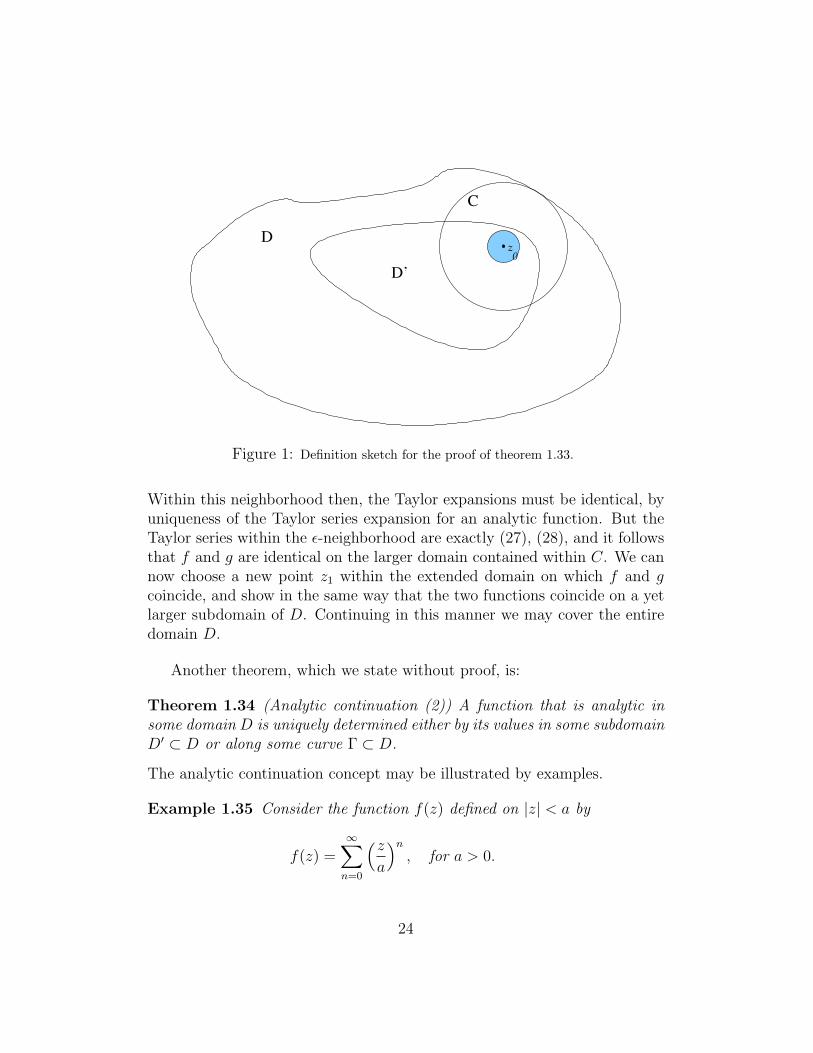
Proof (Sketch) We consider the case in which f and g coincide on a subdo-main D′. Let z0 ∈ D′, and then take the largest circle C ⊂ D, within whichboth f and g are known to be analytic (see figure 1). By Taylor’s theorem25, both f and g have Taylor series expansions
f(z) =∞∑n=0
f (n)(z0)(z − z0)n
n!=∞∑n=0
Cn(z0)(z − z0)n, (27)
g(z) =∞∑n=0
g(n)(z0)(z − z0)n
n!=∞∑n=0
En(z0)(z − z0)n, (28)
that converge inside C. Also, since D′ is open, it contains an ε-neighborhoodof z0 (shaded in the sketch 1), and on which f and g are known to be identical.
23
D
C
D’0z
Figure 1: Definition sketch for the proof of theorem 1.33.
Within this neighborhood then, the Taylor expansions must be identical, byuniqueness of the Taylor series expansion for an analytic function. But theTaylor series within the ε-neighborhood are exactly (27), (28), and it followsthat f and g are identical on the larger domain contained within C. We cannow choose a new point z1 within the extended domain on which f and gcoincide, and show in the same way that the two functions coincide on a yetlarger subdomain of D. Continuing in this manner we may cover the entiredomain D.
Another theorem, which we state without proof, is:
Theorem 1.34 (Analytic continuation (2)) A function that is analytic insome domain D is uniquely determined either by its values in some subdomainD′ ⊂ D or along some curve Γ ⊂ D.
The analytic continuation concept may be illustrated by examples.
Example 1.35 Consider the function f(z) defined on |z| < a by
f(z) =∞∑n=0
(za
)n, for a > 0.
24
This series converges uniformly for |z| < a and so defines an analytic functionin that region, but it diverges for |z| > a and so does not represent an analyticfunction there. However, the function
g(z) =a
a− z
is defined and analytic for all z 6= a, and moreover, for |z| < a we have
g(z) = (1− z/a)−1 =∞∑n=0
(za
)n≡ f(z).
We say that g(z) represents the analytic continuation of f(z) outside thedisc |z| < a. The representation f(z), which is only valid on this subdo-main, is sufficient to determine uniquely the function g(z), valid in the entirecomplex plane minus the single point z = a.
Example 1.36 What is the analytic continuation of the function that takesvalues y3 = y on the imaginary axis z = iy?
An alternative way to phrase this question would be: Find the unique func-tion f(z), complex analytic in some neighborhood of the imaginary axis, suchthat f(z) = y3 − y on the imaginary axis z = iy.
To answer the question, we note that on z = iy, y = −iz, and so theboundary values of f may be re-expressed as
f(z) = iz3 + iz on <(z) = 0.
Since f as defined here is analytic in a neighborhood of the line, and is equalto the given values on the line, the analytic continuation property tells usthat it is the unique analytic continuation of the boundary data away fromthe boundary curve.
Remark Contrast the analytic continuation property, in which both realand imaginary parts of an analytic function are specified on a given curve,with the solutions to Laplace’s equation generated previously by our Pois-son integral formulae. There we saw that specifying only the real part of afunction (analytic on a given domain) on the boundary of the domain wassufficient to determine both real and imaginary parts of the function. Thedifference here is that the analytic continuation we generate by specifying
25
both real and imaginary parts will, in general, have singularities in the do-main of continuation. By contrast, any solutions generated by the Poissonformulae are guaranteed to be analytic in the chosen domain. Analytic con-tinuation is an ill-posed technique mathematically (see, e.g. [8] § 2.3 in thiscontext).
We will use this property later in applications. Another theorem on an-alytic continuation is proved below:
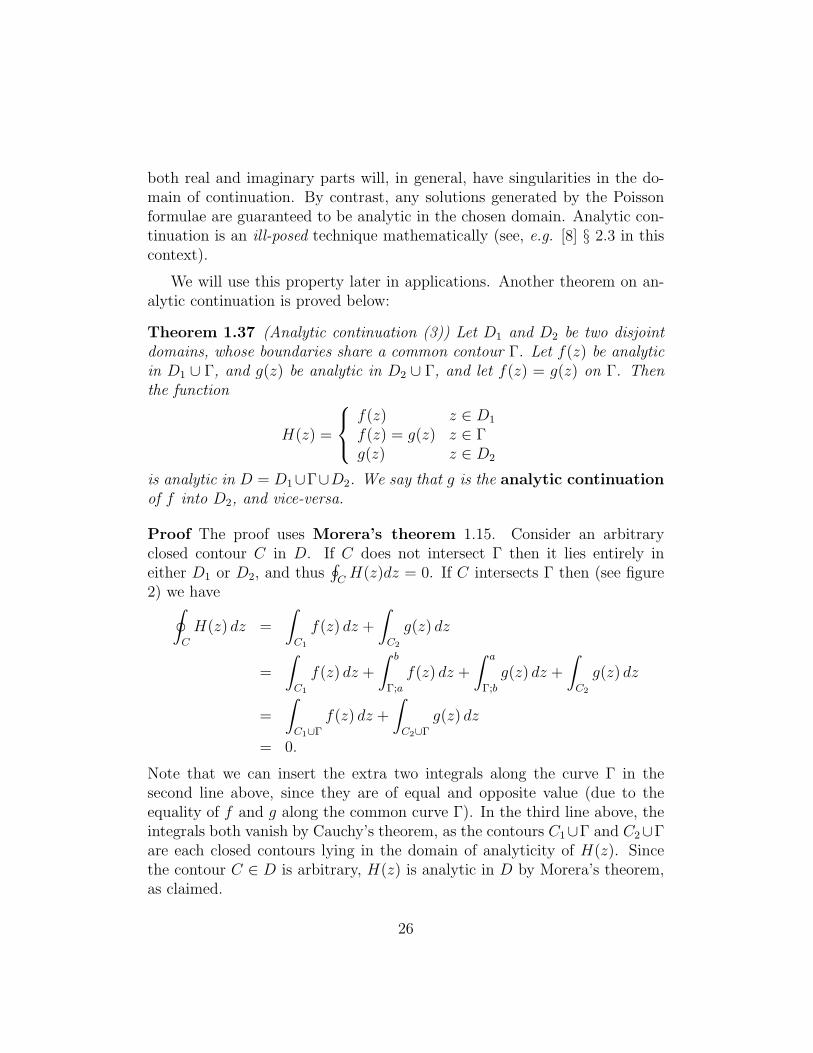
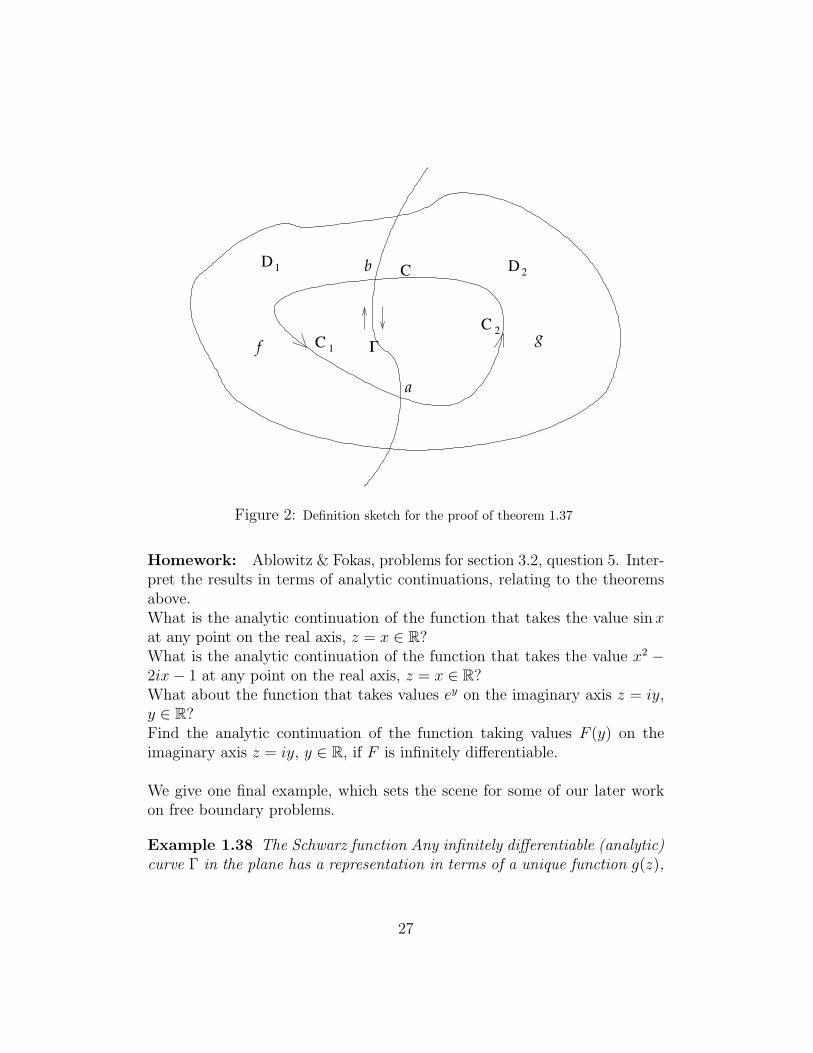
Theorem 1.37 (Analytic continuation (3)) Let D1 and D2 be two disjointdomains, whose boundaries share a common contour Γ. Let f(z) be analyticin D1 ∪ Γ, and g(z) be analytic in D2 ∪ Γ, and let f(z) = g(z) on Γ. Thenthe function
H(z) =
f(z) z ∈ D1
f(z) = g(z) z ∈ Γg(z) z ∈ D2
is analytic in D = D1∪Γ∪D2. We say that g is the analytic continuationof f into D2, and vice-versa.
Proof The proof uses Morera’s theorem 1.15. Consider an arbitraryclosed contour C in D. If C does not intersect Γ then it lies entirely ineither D1 or D2, and thus
∮CH(z)dz = 0. If C intersects Γ then (see figure
2) we have∮C
H(z) dz =
∫C1
f(z) dz +
∫C2
g(z) dz
=
∫C1
f(z) dz +
∫ b
Γ;a
f(z) dz +
∫ a
Γ;b
g(z) dz +
∫C2
g(z) dz
=
∫C1∪Γ
f(z) dz +
∫C2∪Γ
g(z) dz
= 0.
Note that we can insert the extra two integrals along the curve Γ in thesecond line above, since they are of equal and opposite value (due to theequality of f and g along the common curve Γ). In the third line above, theintegrals both vanish by Cauchy’s theorem, as the contours C1∪Γ and C2∪Γare each closed contours lying in the domain of analyticity of H(z). Sincethe contour C ∈ D is arbitrary, H(z) is analytic in D by Morera’s theorem,as claimed.
26
D C
a
b 21
2C
D
f g1C !
Figure 2: Definition sketch for the proof of theorem 1.37
Homework: Ablowitz & Fokas, problems for section 3.2, question 5. Inter-pret the results in terms of analytic continuations, relating to the theoremsabove.What is the analytic continuation of the function that takes the value sin xat any point on the real axis, z = x ∈ R?What is the analytic continuation of the function that takes the value x2 −2ix− 1 at any point on the real axis, z = x ∈ R?What about the function that takes values ey on the imaginary axis z = iy,y ∈ R?Find the analytic continuation of the function taking values F (y) on theimaginary axis z = iy, y ∈ R, if F is infinitely differentiable.
We give one final example, which sets the scene for some of our later workon free boundary problems.
Example 1.38 The Schwarz function Any infinitely differentiable (analytic)curve Γ in the plane has a representation in terms of a unique function g(z),
27
complex analytic in some neighborhood of Γ:
z = g(z) on Γ. (29)
Equation (29) defines the curve. Given the curve (e.g. as an algebraic equa-tion F (x, y) = 0), we know only the values of g on Γ. We can find these bysolving
F
(z + z
2,z − z
2i
)for z. Analytic continuation will then tell us what the function g(z) is atarbitrary points of the complex plane.
To see how this works for some elementary examples, consider the unit circlex2 + y2 = 1. The above formula for extracting the Schwarz function gives
1
4(z + z)2 − 1
4(z − z)2 = 1 → zz = 1, on Γ.
(Of course, we could have written this down right away for this simple exam-ple.) Thus, g(z) = 1/z on Γ, and hence g(z) ≡ 1/z, by analytic continuation(since 1/z is clearly analytic in a neighborhood of Γ).
Homework: Find the Schwarz function of the straight line y = mx + c,for any real constants m, c.
It is not usually so straightforward to extract the Schwarz function of agiven curve! Usually in applications we want to find the Schwarz functionof the curve bounding a given domain D. If D has a complicated boundaryshape then one way to find its Schwarz function is to use the fact (whichwe will explore in detail later) that any simply-connected domain D ⊂ Cmay be recognized as the image, under a 1-1 analytic function (“conformalmapping”), of a nice domain such as the unit disc, B(0; 1). We can write
z ∈ D ⇒ z = f(ζ), |ζ| ≤ 1,
and further, boundary points map to boundary points, so that
z ∈ ∂D ⇒ z = f(ζ), |ζ| = 1.
28
We need one more piece of useful information: given any analytic functionF (w), the function defined by taking F (w) is another analytic function, whichwe write as F (w): the complex conjugate function to F .
To determine the Schwarz function of the boundary curve ∂D, we needto know the values of z on the boundary. We know that a boundary point isthe image of a point ζ on the boundary of the unit circle, |ζ| = 1. Therefore,
z|∂D = f(ζ)||ζ|=1 = f
(1
ζ
)∣∣∣∣|ζ|=1
⇒ z|∂D = f
(1
ζ
)∣∣∣∣∣|ζ|=1
= f
(1
ζ
)∣∣∣∣|ζ|=1
.
As written, this identity holds only gives g(z) on the boundary curve (∂D, or|ζ| = 1), but we know that the function f(1/ζ) is analytic, at least in someneighborhood of the boundary. Therefore, we may analytically continue theidentity away from the boundary, and conclude that
g(z) = f
(1
ζ
),
or equivalently,
g(f(ζ)) = f
(1
ζ
), or g(z) = f
(1
f−1(z)
)(we know the inverse function f−1 exists since f is 1-1).
1.7.1 Natural barriers
There are some types of singularities (non-isolated) that preclude analyticcontinuation. We refer to these singularities as natural barriers of thefunction under consideration. A classic example of a function exhibiting anatural barrier is provided by
f(z) =∞∑n=0
fn =∞∑n=0
z2n . (30)
The ratio test guarantees convergence where limn→∞ fn+1/fn < 1, and
fn+1
fn=z2n+1
z2n=z2n.2
z2n=
(z2n)2
z2n= z2n .
29
This limit is less than one only if |z| < 1, so the series converges on the openunit disc, but f clearly diverges for z = 1. Also,
f(z2) =∞∑n=0
(z2)2n =∞∑n=0
z2(n+1)
=∞∑n=1
z2n =∞∑n=0
z2n − z = f(z)− z,
so f satisfies the functional equation
f(z) = f(z2) + z. (31)
Repeated application of this formula gives
f(z2) = f(z4) + z2
and then substituting in (31) gives
f(z) = f(z4) + z2 + z. (32)
Similarly, replacing z by z4 in (31) gives
f(z4) = f(z8) + z4,
and then substituting in (32) gives
f(z) = f(z8) + z4 + z2 + z.
Continuing in this manner (prove by induction if you wish) we see that fsatisfies
f(z) = f(z2m) +m−1∑n=0
z2n , (33)
for any positive integer m. Since we know f(1) = ∞, this equation tellsus that f is also singular at all points zs,m where z2m
s,m = 1, because at suchpoints (33) gives
f(zs,m) = f(1) +m−1∑n=0
z2n =∞.
Therefore, f is singular at all points
zs,m = e2πis/2m , s = 1, 2, . . . , 2m, for any m ∈ Z.
30
In order to use the analytic continuation principle to extend the domain ofanalyticity of f into |z| ≥ 1 we need (as a minimum) to find some arc of theunit circle (which bounds the known domain of analyticity, |z| < 1) on whichf is analytic. However, any such arc segment, however small, will alwayscontain a 2mth root of unity, for some integer m, and thus a singularity of f .Hence there is no finite arc-length with |z| = 1 on which f is analytic.
Homework: Ablowitz & Fokas, problems for section 3.5, question 4.
2 Cauchy’s Residue theorem (and others) and
Applications
2.1 Cauchy’s Residue Theorem
Knowing more about non-analytic functions, we are in a position to extendCauchy’s theorem 1.14 to situations where the function contains singularitieswithin the contour of integration.
Theorem 2.1 (Cauchy’s Residue theorem) Let f(z) be analytic inside andon a simple closed contour C, except for a finite number of isolated singularpoints z1, z2, . . . , zN inside C. Then∮
C
f(z) dz = 2πiN∑j=1
aj,
where aj is the residue of f(z) at the point z = zj, aj = Res(f(z); zj).
This remarkable theorem has many applications, including the summationof infinite series, and inversion of Laplace transforms. Residues may beevaluated using the following theorem:
Theorem 2.2 (Evaluating residues at poles) If f(z) has a pole of order k atz = z0 then
Res(f(z), z0) =1
(k − 1)!limz→z0
dk−1
dzk−1((z − z0)kf(z)) (34)
31
Proof Direct manipulation of the Laurent expansion of f about z0,
f(z) =∞∑
n=−k
Cn(z − z0)n
yields the result for Res(f(z), z0) = C−1.
2.1.1 Application to summing series
The idea here is to recognise the series to be summed as a sum of residuesat the singularities of an otherwise analytic function. By integrating aroundan appropriate contour on which the function decays suitably as the contourmoves off to infinity, one can then apply the residue theorem to deduce thevalue of the sum of residues. The procedure is best illustrated by examples.
Example 2.3 By evaluation of a suitable contour integral, find the infinitesum
S =∞∑n=1
1
n2.
The trick is to find a function whose residues will lead to the appropriate sumwhen the residue theorem is applied. Consider the function f(z) = cot πz/z2,which has simple poles at the points zn = n for n ∈ Z, (n 6= 0), and a triplepole at the origin. The residues at zn are evaluated by applying (34):
Res(f(z); zn) = limz→n
(z − n)f(z) =cosnπ
n2limz→n
(z − n)
sin πz=
1
πn2.
The residue of the triple pole at z = 0 is also given by (34),
Res(f(z); 0) =1
2limz→0
d2
dz2(z cot πz) = lim
z→0πcosec2πz(πz cot πz − 1) = −π
3.
The Residue theorem 2.1 states that, for a rectangular contour CN composedof the straight lines <(z) = ±(N + 1/2) (so that we avoid the poles of thefunction) and =(z) = ±N (for N ∈ N), we have∮
CN
f(z)dz = 2N∑n=1
1
πn2− π
3. (35)
32
If we let N →∞ then we retrieve the sum S on the right-hand side, in termsof the contour integral.
To evaluate the contour integral we split it into four natural parts alongeach straight-line segment, and show that the size of each integral goes tozero as N →∞.
On the portion <(z) = (N+1/2) we have z = N+1/2+ iy, −N < y < Nand
| cot πz| =∣∣∣∣cos[π(N + 1/2) + iπy]
sin[π(N + 1/2) + iπy]
∣∣∣∣ =
∣∣∣∣ sinh πy
cosh πy
∣∣∣∣ ≤ 1,
and similarly on the portion <(z) = −(N + 1/2).On the portion =(z) = N we have z = x+iN , −(N+1/2) < x < N+1/2
and
| cot πz|2 =
∣∣∣∣cos[πx+ iNπ]
sin[πx+ iNπ]
∣∣∣∣2 =
∣∣∣∣cosπx coshNπ − i sinπx sinhNπ
sin πx coshNπ + i cos πx sinhNπ
∣∣∣∣2=
cos2 πx cosh2Nπ + sin2 πx sinh2Nπ
sin2 πx cosh2Nπ + cos2 πx sinh2Nπ
=cosh2Nπ + sin2 πx
cosh2Nπ + cos2 πx≤ 1 + ε,
where we can take ε as small as we like by taking N sufficiently large (but itis enough for us that we bound it). We can similarly bound | cot πz| by 1 + εon =(z) = −N .
We can therefore make | cotπz| ≤ 2 on all parts of the integration contour,for N sufficiently large, and∣∣∣∣∮CN
f(z)dz
∣∣∣∣ ≤ ∮CN
|f(z)| |dz| ≤ 2
N2
∮CN
|dz| = 4(4N + 1)
N2→ 0 as N →∞.
Letting N →∞ in (35) then gives the result
N∑n=1
1
n2=π2
6.
This general method will work for any sum∑∞
n=1 φ(n), where φ has thefollowing properties:
33
• φ(n) = φ(−n) for n = 1, 2, . . .;
• φ(n) is a rational function;
• φ(z) = O(|z|−2) as |z| → ∞.
The procedure is to integrate f(z) = φ(z)π cot πz around the same rectan-gular contour CN and use the Residue theorem. The term π cotπz givessimple poles of f at each integer n (where φ is nonzero and analytic) ofresidue φ(n). The bound on φ ensures, as in the worked example above, that∫CN
f(z) dz → 0 as N →∞.
Under these same conditions on φ we can evaluate∑∞
n=1(−1)nφ(n) byintegrating f(z) = φ(z)πcosecπz around the same contour CN . The cosecterm leads to a simple pole of residue (−1)nφ(n) at each integer n (againsupposing φ is nonzero and analytic there). The integral around the contourwill go to zero as N →∞, and the Residue theorem will give the result.
Homework: Ablowitz & Fokas, Problems for section 4.2, questions 8 and9.
2.2 Principle of the argument & Rouche’s theorem
Residue calculus can also be applied to deduce results about the number ofzeros and poles of a meromorphic function in a given region.
Theorem 2.4 (Argument principle) Let f be meromorphic inside and on asimple closed contour C, with N zeros inside C, P poles inside C (wheremultiple zeros and poles are counted according to multiplicity), and no zerosor poles on C. Then
1
2πi
∮C
f ′(z)
f(z)dz = N − P =
1
2π[arg(f(z))]C
(the last expression denotes the change in the argument of f as C is traversedonce).
Proof Let zi be a zero/pole of order ni. Then
f(z) = (z − zi)±nigi(z), (+ for zero, − for pole)
34
where gi(zi) 6= 0 and gi(z) is analytic in some neighborhood B(zi, εi) of zi.Thus in such a neighborhood we can write
f ′(z)
f(z)=±ni
(z − zi)+ φi(z)
where φi(z) = g′i(z)/gi(z) is analytic in B(zi, εi), and in the region D′ madeup of the interior of the curve C, with each B(zi, εi) removed, f ′/f is analytic.Application of Cauchy’s theorem 1.14 to the region D′ then gives
0 =1
2πi
∮∂D′
f ′(z)
f(z)dz
=1
2πi
∮C
f ′(z)
f(z)dz − 1
2πi
∑i
∮γ(zi,εi)
f ′(z)
f(z)dz
=1
2πi
∮C
f ′(z)
f(z)dz − 1
2πi
∑i
∮γ(zi,εi)
±ni(z − zi)
+ φi(z)dz
⇒ 1
2πi
∮C
f ′(z)
f(z)dz =
∑zeros
ni −∑poles
nj = N − P,
where γ(zi, εi) denotes the circle of center zi and radius εi, and we used theresidue theorem 2.1 in the last step. The quantities N , P are as defined inthe theorem statement.
To demonstrate the final equality in the theorem, we parametrize thecurve C so that
C = {z(t) : t ∈ [a, b], z(a) = z(b)}.
Then
1
2πi
∮C
f ′(z)
f(z)dz =
1
2πi
∫ b
a
f ′(z(t))
f(z(t))z′(t)dt =
1
2πi[log|f(z(t))|+ i arg(f(z(t)))]bt=a
=1
2π[arg(f(z))]C
(which branch of the logarithm we choose is immaterial for the theoremresult, but for definiteness you can assume the principal branch).
The theorem has an interesting geometrical interpretation. The functionw = f(z) represents a mapping from the complex z-plane to the complex w-plane, under which the curve C maps to some image curve C ′ in the w-plane
35
(see later notes on conformal mappings). We then have dw = f ′(z)dz, sothat
1
2πi
∮C
f ′(z)
f(z)dz =
1
2πi
∮C′
dw
w=
1
2πi[log(w)]C′ =
1
2π[arg(w)]C′ .
Remark This quantity (1/2π)[arg(w)]C′ is known as the winding numberof the curve C ′ about the origin in the w-plane – the number of times thatthe closed curve C ′ encircles the origin. More generally we have:
Definition 2.5 (Winding number) Let γ be a piecewise-smooth closed con-tour in the w-plane, and w0 ∈ C a point in the w-plane. Then the quantity
n(γ, w0) =1
2πi
∮γ
dw
(w − w0)
is known as the winding number of the curve γ about the point w0.
Parametrizing γ as before by t ∈ [a, b],
γ = {w(t) : t ∈ [a, b], w(a) = w(b)},
we have
n(γ, w0) =1
2πi
∫ b
a
w′(t)dt
(w(t)− w0)=
1
2πi[log(w(t)− w0)]ba =
1
2π[arg(w − w0)]γ,
which, geometrically, represents the number of times that the curve γ encir-cles the point w0 ∈ C. (Note: for the sake of brevity this argument assumesthat γ is smooth, but it is easily extended to the case of piecewise smoothγ.)
This concept provides us with an alternative way of defining a simply-connected domain:
Definition 2.6 A domain D ⊂ C is called simply connected if it has theproperty that, for all w0 6∈ D and for every piecewise-smooth closed contourγ ∈ D, we have n(γ, w0) = 0.
Example 2.7 Find the number of zeros of the function f(z) = z5 + 1 withinthe first quadrant.
36
We use the principle of the argument to determine the change in arg(f) aswe traverse an appropriate contour. Since f is analytic on the first quadrantof the z-plane, we may take the contour C to be a large quarter-circle, madeup of the three portions C = C1 ∪ C2 ∪ C3,
C1 = {z : z = x, 0 ≤ x ≤ R},C2 = {z : z = Reiθ, 0 ≤ θ ≤ π/2},C3 = {z : z = iy, 0 ≤ y ≤ R}.
In the limit that R becomes arbitrarily large the contour will enclose thewhole of the first quadrant. The argument of f satisfies arg(f) = φ, wheretanφ = =(f)/<(f). Along C1 f = 1 + x5 ∈ R+, and arg(f) = 0. AlongC2 f = 1 + R5e5iθ ≈ R5e5iθ, and the argument of f therefore increases from0 to 5π/2 (in the limit R → ∞) as θ increases from 0 to π/2. Finally,on C3 f = 1 + iy5, and for y = R � 1 we have arg(f) ≈ 5π/2 (it mustvary continuously from C2 to C3), while as y decreases from R � 1 to 0,tanφ = =(f)/<(f) decreases (continuously) from +∞ to 0+ and thus arg(f)decreases (continuously) from 5π/2 to 2π.
Thus, the net change in arg(f) as we traverse C is 2π. Applying theorem2.4 then, since f has no singularities within the first quadrant (so P = 0),the number of zeros it has, N , satisfies
N =1
2π[arg(f)]C =
2π
2π= 1.
Theorem 2.8 (Rouche) Let f(z) and g(z) be analytic inside and on a simpleclosed contour C. If |f | > |g| on C, then f and f + g have the same numberof zeros inside C.
This theorem makes sense intuitively, since we can think of g as beinga perturbation to f , which will in turn perturb its zeros. If the size of theperturbation is bounded on the contour C, then (we can show) the size ofthe perturbation is bounded inside C as well (this is not surprising, giventhe maximum modulus principle for analytic functions). Therefore, we havenot perturbed the zeros of f too much by adding g.
Proof Since |f | > |g| ≥ 0 on C it follows that |f | > 0 on C and thus f 6= 0on C. Moreover, f(z) + g(z) 6= 0 on C. Let
h(z) =f(z) + g(z)
f(z),
37
then h is analytic and nonzero on C, and the Argument Principle theorem2.4 may be applied to deduce that
1
2πi
∮C
h′(z)
h(z)dz =
1
2π[arg(w)]C′ ,
where w = h(z), and C ′ is the image of the curve C under this transformationin the w-plane. However,
w = h(z) = 1 +g(z)
f(z)
so, since |g| < |f | on C, we have |w − 1| < 1 on C ′, so that all points ofC ′ lie within the circle of radius 1 centered at w = 1. Thus, as we traversethe closed curve C ′ there is no net change in arg(w), because C ′ does notenclose the origin. It follows from the argument principle that Nh − Ph = 0,where Nh and Ph are the numbers of zeros and poles, respectively (countedaccording to multiplicity) of h(z). Since f and g are analytic inside and onC, the poles of h coincide in location and multiplicity with the zeros of f , sothat Ph = Nf . Also by analyticity of f , h is zero only where f + g = 0, andwe have Nh = Nf+g. Thus,
Nh − Ph = 0 ⇒ Nf = Nf+g,
and the theorem is proved.
Example 2.9 Show that 4z2 = eiz has a solution on the unit disc |z| ≤ 1.
Take the contour C to be |z| = 1, so that points on C are given by z = eit,t ∈ [0, 2π]. Then, with f(z) = 4z2 and g(z) = −eiz, we have |f | = 4 on C,while
|g(z)|C = |ei(cos t+i sin t)| = e− sin t ≤ e < |f(z)|C .
Thus Rouche’s theorem applies, and f + g has the same number of zeros asf on the unit disc. Clearly, f(z) = 4z2 has exactly 2 zeros (both at z = 0but we count according to multiplicity). It follows that 4z2 = eiz in fact has2 solutions on the unit disc.
Homework: Ablowitz & Fokas, problems for section 4.4, questions 3(b),5(a).
38
2.3 Integral transform methods
Two common and useful integral transforms that can be used to solve com-plicated partial differential equations and integro-differential equations arethe Fourier Transform and the Laplace Transform. We shall briefly considerboth of these transforms here, focusing particularly on the Laplace Trans-form, and use of the calculus of residues to invert this transform. However,we begin our discussion with the Fourier transform, of which the Laplacetransform may be considered a special case.
2.3.1 Fourier Transform
Motivation (non-rigorous) Recall the definition of the Fourier seriesof a function f , defined on the real interval −T ≤ t ≤ T ,
f(t) =a0
2+∞∑n=1
(an cos
(nπt
T
)+ bn sin
(nπt
T
)), (36)
where an and bn are given by
an =1
T
∫ T
−Tf(τ) cos
(nπτT
)dτ, bn =
1
T
∫ T
−Tf(τ) sin
(nπτT
)dτ,
so that (substituting for an, bn in (36))
f(t) =1
2T
∫ T
−Tf(τ)dτ +
∞∑n=1
1
T
∫ T
−Tf(τ) cos
(nπ(τ − t)
T
)dτ
=∞∑−∞
1
2T
∫ T
−Tf(τ) cos
(nπ(τ − t)
T
)dτ.
If we set nπ/T = kn, and π/T = kn+1 − kn = δkn, then the process T →∞formally yields the result
f(t) =1
2π
∫ ∞−∞
dk
∫ ∞−∞
f(τ) cos k(τ − t) dτ (37)
a version of the Fourier integral theorem. Since the integrand is even ink, we can rewrite (37) as
f(t) =1
π
∫ ∞0
dk
∫ ∞−∞
f(τ) cos k(τ − t) dτ. (38)
39
Alternatively, since sin k(τ − t) is odd in k, we can rewrite (37) as
f(t) =1
2π
∫ ∞−∞
dk
∫ ∞−∞
f(τ)eik(τ−t) dτ. (39)
Equations (37), (38) and (39) are equivalent. If we then define the Fouriertransform of f by
f(k) =1√2π
∫ ∞−∞
eikτf(τ)dτ, (40)
equation (39) provides the inversion formula
f(t) =1√2π
∫ ∞−∞
e−iktf(k) dk. (41)
For a large class of functions the Fourier transform f(k) defined in (40) is ananalytic function of the complex variable k. We shall now prove the result(41) for a certain class of functions (though in fact the result extends to afar greater class than we shall prove it for).
Theorem 2.10 (Fourier’s Integral Theorem) Let f(t) be a piecewise smoothfunction of the real variable t, with |f | integrable on (−∞,∞). Then
f(t) =1
2π
∫ ∞−∞
dk
∫ ∞−∞
f(τ)eik(τ−t)dτ,
so that if the Fourier transform f(k) is defined by
f(k) =1√2π
∫ ∞−∞
eikτf(τ) dτ,
then the inversion formula is given by
f(t) =1√2π
∫ ∞−∞
e−iktf(k) dk.
The proof will use the following Lemma:
Lemma 2.11 For any 0 < T <∞ and piecewise smooth f ,
limL→∞
∫ T
−Tf(t+ τ)
sinLτ
τdτ =
π
2[f(t+) + f(t−)], (42)
where f(t+), f(t−) denote the limits of f(t+ ε), f(t− ε) as ε→ 0 (ε > 0).
40
Proof To prove the lemma we split the range of integration on the left-handside of (42) into positive and negative τ :
∫ 0
−T +∫ T
0. For the positive range
we write∫ T
0
f(t+ τ)sinLτ
τdτ =
∫ T
0
[f(t+ τ)− f(t+)]sinLτ
τdτ +
f(t+)
∫ T
0
sinLτ
τdτ. (43)
Then, in the second integral on the right-hand side above,
limL→∞
f(t+)
∫ T
0
sinLτ
τdτ = f(t+) lim
L→∞
∫ LT
0
sinx
xdx =
f(t+)
∫ ∞0
sinx
xdx =
π
2f(t+). (44)
Returning to the first integral on the right-hand side of (43), the piecewisesmoothness of f implies that f ′(t+) exists, and thus given ε > 0 there existsh > 0 such that for 0 < τ < h,
f(t+ τ)− f(t+)
τ= f ′(t+) + g(τ),
with |g(τ)| < ε. Hence,∫ T
0
[f(t+ τ)− f(t+)]sinLτ
τdτ =∫ h
0
[f ′(t+) + g(τ)] sinLτ dτ +
∫ T
h
[f(t+ τ)− f(t+)]sinLτ
τdτ. (45)
We now prove the following
Claim 2.12 For a function w piecewise continuous on an interval (a, b),∫ b
a
w(τ) sinLτ dτ → 0 as L→∞.
To show this let δ > 0 be arbitrarily small, and divide up the interval (a, b)into N(δ) increments τk < τ < τk+1 (τ0 = a, τN = b) such that on eachsubinterval τk < τ < τk+1, w can be approximated arbitrarily closely by
41
some constant Ak, in the sense that, for the piecewise constant approximatingfunction v defined by
v(τ) =
A1 a = τ0 < τ < τ1
A2 τ1 < τ < τ2
. . . . . .AN τN−1 < τ < τN = b,
we have ∫ b
a
|w(τ)− v(τ)|dτ < δ
2.
Then, for any L, we have∣∣∣∣∫ b
a
w(τ) sinLτ dτ
∣∣∣∣− ∣∣∣∣∫ b
a
v(τ) sinLτ dτ
∣∣∣∣ ≤ ∣∣∣∣∫ b
a
(w(τ)− v(τ)) sinLτ dτ
∣∣∣∣≤
∫ b
a
|w(τ)− v(τ)| dτ < δ
2.
From this it follows that∣∣∣∣∫ b
a
w(τ) sinLτ dτ
∣∣∣∣ <δ
2+
∣∣∣∣∫ b
a
v(τ) sinLτ dτ
∣∣∣∣=
δ
2+
∣∣∣∣∣N−1∑k=0
Ak+1
∫ τk+1
τk
sinLτ dτ
∣∣∣∣∣≤ δ
2+
2NM
L,
where M = max{Ak}. For δ fixed and arbitrarily small (and N depends onlyon δ while M can be an independent bound), if we choose L > 4MN/δ thenwe have ∣∣∣∣∫ b
a
w(τ) sinLτ dτ
∣∣∣∣ < δ;
that is, the integral can be made arbitrarily small by choosing L sufficientlylarge, and hence it must go to zero as L→∞, which proves the claim.
Returning to (45), we see that the result of the claim applies to each ofthe integrals on the right-hand side, since the functions premultiplying sinLτ
42
are piecewise continuous on the range of integration in each case. It followsthat each of these integrals tends to zero as L→∞, and hence∫ T
0
[f(t+ τ)− f(t+)]sinLτ
τdτ → 0 as L→∞. (46)
Using (44) and (46) in (43), we obtain
limL→∞
∫ T
0
f(t+ τ)sinLτ
τdτ =
π
2f(t+).
A similar result holds for the integral over the negative range of τ -values,
limL→∞
∫ 0
−Tf(t+ τ)
sinLτ
τdτ =
π
2f(t−),
and putting these two results together completes the proof of Lemma 2.11.
We are now in a position to prove theorem 2.10.
Proof (Fourier Integral Theorem) We shall prove that
limL→∞
∫ L
0
dk
∫ ∞−∞
f(t+ τ) cos kτ dτ =π
2[f(t+) + f(t−)] (47)
which is equivalent to the identity (38), which in turn is equivalent to (37)and (39). Let T1 > T > 0. Then∫ L
0
dk
∫ T1
−T1
f(t+ τ) cos kτ dτ −∫ L
0
dk
∫ T
−Tf(t+ τ) cos kτ dτ =∫ −T
−T1
f(t+ τ)sinLτ
τdτ −
∫ T1
T
f(t+ τ)sinLτ
τdτ, (48)
performing the integral with respect to k. Since we assume |f | is integrable,K =
∫∞−∞ |f(τ)dτ | <∞, and thus from (48) above we have∣∣∣∣∫ L
0
dk
∫ T1
−T1
f(t+ τ) cos kτdτ −∫ L
0
dk
∫ T
−Tf(t+ τ) cos kτdτ
∣∣∣∣=
∣∣∣∣∫ −T−T1
f(t+ τ)sinLτ
τdτ −
∫ T1
T
f(t+ τ)sinLτ
τdτ
∣∣∣∣43
≤∣∣∣∣∫ −T−T1
f(t+ τ)sinLτ
τdτ
∣∣∣∣+
∣∣∣∣∫ T1
T
f(t+ τ)sinLτ
τdτ
∣∣∣∣≤
∫ −T−T1
∣∣∣∣f(t+ τ)
τ
∣∣∣∣ dτ +
∫ T1
T
∣∣∣∣f(t+ τ)
τ
∣∣∣∣ dτ<
1
T
∫ ∞−∞|f(t+ τ)|dτ =
K
T.
Thus, letting T1 →∞,∣∣∣∣∫ L
0
dk
∫ ∞−∞
f(t+ τ) cos kτ dτ −∫ L
0
dk
∫ T
−Tf(t+ τ) cos kτ dτ
∣∣∣∣ < K
T. (49)
The second expression on the left-hand side here can be written (as above,by performing the integral with respect to k) as∫ L
0
dk
∫ T
−Tdτ =
∫ T
−Tf(t+ τ)
sinLτ
τdτ → π
2[f(t+) + f(t−)] as L→∞,
by Lemma 2.11. Using this in (49) gives, as L→∞,∣∣∣∣ limL→∞
∫ L
0
∫ ∞−∞
f(t+ τ) cos kτ dτdk − π
2[f(t+) + f(t−)]
∣∣∣∣ < K
T.
However T here is arbitrary, so letting it become large we establish equation(47).
Summary: We have proved that, if the Fourier transform of a piecewisesmooth function f(t), t ∈ (−∞,∞), where also |f | is integrable, is definedby
f(k) =1√2π
∫ ∞−∞
eikτf(τ) dτ (50)
then the inversion formula gives f(t) as
f(t) =1√2π
∫ ∞−∞
e−iktf(k) dk. (51)
As observed earlier however, in fact these formulae are good for a much widerclass of functions f(t).
44
The Fourier Transform and its inverse are sometimes also written as operatorsacting on the functions,
F [f(t)] = f(k) =1√2π
∫ ∞−∞
eikτf(τ) dτ,
F−1[f(k)
]= f(t) =
1√2π
∫ ∞−∞
e−iktf(k) dk.
Evaluation of the inverse Fourier transform can often be accomplished viacomplex contour integration.
Example 2.13 Verify the result of the Fourier Integral theorem for the func-tion f defined by
f(t) =
{e−at t > 0,ebt t < 0,
(52)
where a, b ∈ R+.
Finding the Fourier transform is straightforward:
f(k) =1√2π
∫ 0
−∞ebτ+ikτ dτ +
1√2π
∫ ∞0
e−aτ+ikτ dτ
=1√2π
[ebτ+ikτ
b+ ik
]0
−∞− 1√
2π
[e−aτ+ikτ
a− ik
]∞0
=1√2π
(1
a− ik+
1
b+ ik
).
To reconstruct f from f(k) we must evaluate the inversion integral (51),which gives
f(t) =1
2π
∫ ∞−∞
e−ikt(
1
a− ik+
1
b+ ik
)dk, (53)
and this may be done using the Residue theorem on a large closed semicircularcontour if we note that, for t > 0, the integrand decays for k = Reiθ =R(cos θ+ i sin θ) where π < θ < 2π, while for t < 0, the integrand decays fork = Reiθ = R(cos θ + i sin θ) where 0 < θ < π. For values t > 0 we thereforeuse a large semicircular contour in the lower-half k-plane, C−, while fort < 0 we use a large semicircle in the upper-half k-plane, C+.
45
Considering each term in the inversion integral (53) separately we have,for t > 0,
1
2π
∫ ∞−∞
e−ikt
a− ikdk = − 1
2π
∮C−
e−ikt
a− ikdk +
1
2π
∫Γ−
e−ikt
a− ikdk, (54)
where Γ− = {k : k = Reiθ : π < θ < 2π} is the curved portion of C−. Forthe integral around C− the Residue theorem (2.1) applies, giving∮
C−
e−ikt
a− ikdk = 2πiRes(e−ikt/(a− ik);−ia) = 2πi(−ie−at) = 2πe−at;
the only singularity of the integrand inside C− being at k = −ia; while onΓ− we have ∣∣∣∣∫
Γ−
e−ikt
a− ikdk
∣∣∣∣ =
∣∣∣∣∫ 2π
π
eRt(sin θ−i cos θ)iReiθ
a− iReiθdθ
∣∣∣∣≤ R
R− a
∫ 2π
π
eRt sin θdθ
=R
R− a
∫ π
0
e−Rt sinφdφ
=2R
R− a
∫ π/2
0
e−Rt sinφdφ.
By Jordan’s inequality we have 2φ/π ≤ sinφ ≤ φ for 0 ≤ φ ≤ π/2, and thus∣∣∣∣∫Γ−
e−ikt
a− ikdk
∣∣∣∣ ≤ 2R
R− a
∫ π/2
0
e−2Rtφ/πdφ =π
t(R− a)(1− e−Rt)→ 0 as R→∞.
Returning to (54) then, for t > 0 the inverse Fourier transform of 1/(√
2π(a−ik)) is
1
2π
∫ ∞−∞
e−ikt
a− ikdk = e−at, t > 0.
For t < 0 similar arguments may be applied to the inversion integral usingthe semicircular contour C+ in the upper-half k-plane; here the singularityat k = −ia lies outside the contour of integration and so∮
C+
e−ikt
a− ikdk = 0,
46
giving the inverse Fourier transform of 1/(√
2π(a− ik)) for t < 0 as
1
2π
∫ ∞−∞
e−ikt
a− ikdk = 0, t < 0.
For t = 0 finally, we have (interpreting the inversion integral in the prin-cipal value sense, and again using the contour C+ in the upper-half k-plane composed of the real line −R ≤ <(k) ≤ R and the circular arcΓ+ = {k : k = Rei/θ, 0 < θ < π})
1
2π
∫ ∞−∞
e−ikt
a− ikdk =
1
2πlimR→∞
∫ R
−R
1
a− ikdk
=1
2πlimR→∞
(∮C+
1
a− ikdk −
∫Γ+
1
a− ikdk
)= − 1
2πlimR→∞
∫ π
0
iReiθ
a− iReiθdθ
=1
2πlimR→∞
∫ π
0
dθ
1 + iae−iθ/R
= 1/2.
Thus the inverse Fourier transform of 1/(√
2π(a− ik)) over all ranges of t isgiven by
1
2π
∫ ∞−∞
e−ikt
a− ikdk =
e−at t > 01/2 t = 00 t < 0.
(55)
Exactly similar methods apply to the second term in the inversion in-tegral (53) (Exercise: try doing this explicitly), giving the inverse Fouriertransform of 1/(
√2π(b+ ik)) as
1
2π
∫ ∞−∞
e−ikt
b+ ikdk =
0 t > 01/2 t = 0ebt t < 0
(56)
(the pole in the inversion integrand here is at k = ib, inside C+, so we pick upthe nonzero residue contribution when doing this integral for the case t < 0).
Note that the original function (52) is only defined away from t = 0, butthe operation of taking the Fourier transform and inverting gives a valueF−1 [F [f(t)]]t=0 = 1. This is in line with the result of theorem 2.10, whichstates that the operation of inverting the Fourier transform should lead tothe average value, (f(0+) + f(0−))/2, at t = 0.
47
Homework: Ablowitz & Fokas, problems for section 4.5, questions 1,2.
Some key properties of the Fourier Transform:
1. Linearity: F [c1f1(t) + c2f2(t)] = c1F [f1(t)] + c2F [f2(t)].
2. Fourier transform of a derivative:
F[dnf
dtn(t)
]= (−ik)nf(k). (57)
This follows from straightforward integration by parts, assuming thatthe derivatives decay appropriately at infinity:
F[dnf
dtn(t)
]=
1√2π
∫ ∞−∞
eikτdnf
dτn(τ) dτ
=1√2π
{[eikτ
dn−1f
dτn−1
]∞−∞−∫ ∞−∞
(ik)eikτdn−1f
dτn−1dτ
}= (−ik)F
[dn−1f
dtn−1(t)
].
Repeating the argument leads to the result (57).
3. Fourier transform of a product: This is not the product of the Fouriertransforms, but is the convolution of the Fourier transforms,
F [f(t)g(t)] =1√2π
∫ ∞−∞
eikτf(τ)g(τ) dτ
= (f ∗ g)(k)
=1√2π
∫ ∞−∞
f(k − k′)g(k′) dk′. (58)
The result is most easily demonstrated by using the inversion formula(51) on the convolution integral (58) to show we get the product of thefunctions f and g.
F−1[(f ∗ g)(k)
]=
1√2π
∫ ∞−∞
e−ikt(f ∗ g)(k) dk
=1
2π
∫ ∞−∞
e−ikt∫ ∞−∞
f(k − k′)g(k′) dk′ dk
48
=1
2π
∫ ∞−∞
∫ ∞−∞
e−i(k−k′)tf(k − k′)e−ik′tg(k′) dk′ dk
=1
2π
∫ ∞−∞
∫ ∞−∞
e−iκtf(κ)e−ik′tg(k′) dκ dk′
=
(1√2π
∫ ∞−∞
e−iκtf(κ) dκ
)(1√2π
∫ ∞−∞
e−ik′tg(k′) dk′
)= f(t)g(t).
4. In exactly the same way we can demonstrate that the Fourier trans-form of a convolution of two functions is the product of the Fouriertransforms. If
(f ∗ g)(t) =1√2π
∫ ∞−∞
f(t− τ)g(τ) dτ
then
F [(f ∗ g)(t)] = f(k)g(k).
Remark Note that the convolution integral (59) may also be expressedas
(f ∗ g)(t) =1√2π
∫ ∞−∞
f(τ)g(t− τ) dτ.
Exercise: Show this, starting from (59).
Such results make the Fourier transform (and the closely-related Laplacetransform which we discuss below) very useful for solving certain partial orordinary differential equations. Consider the equation
d2u
dt2− ω2u = −f(t), u→ 0 as |t| → ∞,
where ω > 0. Taking the Fourier transform in t gives, using property 2 above,
(k2 + ω2)u(k) = f(k) ⇒ u(k) =f(k)
k2 + ω2= f(k)g(k),
a product of Fourier transforms, so the solution (by property 4 above) is theconvolution of f(t) with g(t),
u(t) =1√2π
∫ ∞−∞
f(t− τ)g(τ) dτ. (59)
49
To find g(t) note that
g(k) =1
k2 + ω2=
1
2ω
(1
ω − ik+
1
ω + ik
)=
√2π
2ωF [G(t)], (60)
where, by the result of example 2.13,
G(t) =
{e−ωt t > 0eωt t < 0
}= e−ω|t|. (61)
Hence finally, by (59), (60) and (61), the solution is
u(t) =1
2ω
∫ ∞−∞
f(t− τ)e−ω|τ |dτ.
In this example we saved time by recognising the function g(k) appearing inthe solution as the Fourier transform of a known function. In fact, since theFourier transform and its inverse are one-to-one transformations, so that theyform a unique pair, this is a very common method of inverting the transform.Extensive tables of Fourier transform pairs exist, examples of which may befound in [2, 5, 10].
Homework: Use the Fourier transform in x to solve the heat equation
ut = αuxx, −∞ < x <∞, t > 0,
u→ 0 as |x| → ∞, u(x, 0) = Be−βx2
, B, β ∈ R+.
Note: take care not to confuse the variables; here you are transforming withrespect to x, not t!
2.3.2 Laplace Transform
Closely related to the Fourier transform is another widely-used exponentialtransform of a function f(t), the Laplace transform.
Definition 2.14 (Laplace Transform) The Laplace transform of a functionf(t) is defined by
L[f(t)] = f(s) =
∫ ∞0
e−stf(t) dt. (62)
50
This transform generally takes a real function of a real variable, f(t), to acomplex function of a complex variable, f(s). Note that if we identify s with(−ik) and define
F (t) =
{f(t) t > 0,0 t < 0,
then
f(s) =√
2πF (is). (63)
Therefore, we will be able to deduce results about the Laplace transform fromthose for the Fourier transform. We first prove that the Laplace transformis an analytic function of s, under appropriate conditions.
Theorem 2.15 If f(t) is piecewise continuous for t ≥ 0, and there existconstants M, σ0, T0 > 0 such that
|f(t)| < Meσ0t ∀t > T0,
then f(s) exists and is analytic on <(s) > σ0.
Remark Note that, of course, the domain of analyticity of f(s) may belarger than this. The theorem simply guarantees analyticity at least withinthis region.
Proof There are many ways of showing this. First we show that the trans-form exists when the conditions are satisfied. Defining fT (s) by
fT (s) =
∫ T
0
e−stf(t) dt
we have f(s) = limT→∞ fT (s), and
|fT (s)| =
∣∣∣∣∫ T0
0
e−stf(t) dt+
∫ T
T0
e−stf(t) dt
∣∣∣∣≤
∣∣∣∣∫ T0
0
e−stf(t) dt
∣∣∣∣+
∣∣∣∣∫ T
T0
e−stf(t) dt
∣∣∣∣≤ K1 +
∫ T
T0
|e−st||f(t)| dt
≤ K1 +M
∫ T
0
e−(<(s)−σ0)t dt
= K1 +M1− e−(<(s)−σ0)T
<(s)− σ0
.
51
Clearly then, for <(s) > σ0, fT (s) exists for all T , including in the limitT →∞, and thus the Laplace transform exists under the stated conditions.
To prove analyticity, we can demonstrate differentiability at all points.Let
Dδ =fT (s+ δ)− fT (s)
δ=
∫ T
0
f(t)e−st(e−δt − 1)
δdt.
Then, for fixed T ,
D := limδ→0
Dδ =
∫ T
0
f(t)e−st(−t)dt,
wherever this integral converges. By arguments similar to those used above,we can show that D exists for <(s) > σ0, for all T , because
|D| =
∣∣∣∣∫ T0
0
e−sttf(t) dt+
∫ T
T0
e−sttf(t) dt
∣∣∣∣≤
∣∣∣∣∫ T0
0
e−sttf(t) dt
∣∣∣∣+
∣∣∣∣∫ T
T0
e−sttf(t) dt
∣∣∣∣≤ K2 +
∫ T
T0
t|e−st||f(t)| dt
≤ K2 +M
∫ T
0
te−(<(s)−σ0)t dt
= K2 +M
((−T )e−(<(s)−σ0)T
<(s)− σ0
+(1− e−(<(s)−σ0)T )
(<(s)− σ0)2
),
where integration by parts was used to derive the last equality. Thus, thederivative f ′T (s) exists for any T > 0, including in the limit T → ∞. Itfollows that f ′(s) exists for any <(s) > σ0, and hence that f(s) is analyticon <(s) > σ0.
Example 2.16 Find the Laplace transform of f(t) = tn, for n ∈ N.
Let
In = f(s) =
∫ ∞0
e−sttn dt.
52
Then, for <(s) > 0, integration by parts gives
In =
[tne−st
(−s)
]∞0
+
∫ ∞0
ntn−1
se−st dt =
n
sIn−1.
Repeating the argument we find
In =n!
snI0 =
n!
sn+1= f(s). (64)
This is analytic for <(s) > 0, as we expect from theorem 2.15.
Example 2.17 Find the Laplace transform of f(t) = sin at.
We again integrate by parts, for <(s) > 0, to obtain
I =
∫ ∞0
e−st sin at dt =
[−e−st
acos at
]∞0
−∫ ∞
0
se−st
acos at dt
=1
a− s
a
{[e−st
asin at
]∞0
+
∫ ∞0
se−st
asin at dt
}=
1
a− s2
a2I.
Rearranging, we find that
I = f(s) =a
a2 + s2.
2.3.3 Properties of Laplace transform
1. Linearity: L[c1f1(t) + c2f2(t)] = c1L[f1(t)] + c2L[f2(t)].
2. Shifting in s: L[eatf(t)] = f(s− a).
L[eatf(t)] =
∫ ∞0
f(t)e−(s−a)t dt = f(s− a).
3. Laplace transform of a derivative: If f is n-times differentiable on t > 0and |f(t)e−st| → 0 as t → ∞ for <(s) > σ0 (some σ0 ∈ R), then for<(s) > σ0 we have
L[dnf
dtn(t)
]= snf(s)− sn−1f(0)− sn−2f ′(0)− · · · − f (n−1)(0). (65)
53
Proof: Let In(s) = L[f (n)(t)]. Then
In(s) =
∫ ∞0
f (n)(t)e−st dt =[f (n−1)(t)e−st
]∞0
+
∫ ∞0
sf (n−1)(t)e−st dt.
The behavior of |f(t)e−st| as t→∞ will also guarantee that f (j)(t)e−st →0 as t→∞ for <(s) > σ0, for j ≥ 1, and thus
In(s) = −f (n−1)(0) + sIn−1(s)
= −f (n−1)(0) + s[−f (n−2)(0) + sIn−2(s)]
= · · · = −f (n−1)(0)− sf (n−2)(0)− s2f (n−3)(0) · · ·+ snI0(s).
Since I0(s) is just f(s), the result follows.
4. Derivative of a Laplace transform: Where f(s) is defined and analyticwe have
L[tnf(t)] = (−1)ndnf
dsn(s). (66)
Proof: Since f(s) is analytic we can differentiate in the definition toobtain
dnf
dsn(s) =
∫ ∞0
f(t)dn
dsn(e−st) dt =
∫ ∞0
(−t)nf(t)e−st dt = (−1)nL[tnf(t)],
as claimed.
5. Laplace transform of an integral: Where g(t) =∫ t
0f(t) dt is defined for
all t, and |g(t)e−st| → 0 as t → ∞ for <(s) > σ0 (some σ0 ∈ R), thenfor <(s) > σ0 we have
L[∫ t
0
f(τ) dτ
]=f(s)
s. (67)
Proof: Integrating by parts in the definition gives
L[∫ t
0
f(τ) dτ
]=
∫ ∞0
(∫ t
0
f(τ) dτ
)e−st dt
=
[(∫ t
0
f(τ) dτ
)e−st
(−s)
]∞0
+
∫ ∞0
f(t)e−st
sdt
=f(s)
s.
54
6. Laplace transform of a convolution:
L [(f ∗ g)(t)] = L[∫ t
0
f(t− τ)g(τ) dτ
]= f(s)g(s). (68)
Proof: Assume f and g are such that Fubini’s theorem is applicableto f(t − τ)g(τ)e−st on the region D = {(τ, t) : 0 < τ < t < ∞} in(τ, t)-space.2 Then the order of the integration may be interchanged,and thus
L[∫ t
0
f(t− τ)g(τ) dτ
]=
∫ ∞0
(∫ t
0
f(t− τ)g(τ) dτ
)e−st dt
=
∫ ∞0
∫ ∞τ
f(t− τ)e−s(t−τ)g(τ)e−sτ dtdτ.
Set t = t− τ in the first t-integral, so that dt = dt. Then
L[∫ t
0
f(t− τ)g(τ) dτ
]=
∫ ∞0
(∫ ∞0
f(t)e−st dt
)g(τ)e−sτ dτ
=
∫ ∞0
f(s)g(τ)e−sτ dτ = f(s)g(s).
Example 2.18 Solve the following integro-differential equation, subject toboundary conditions f(0) = 0, f(π) =
√2.∫ t
0
f(τ) dτ + 4tf(t) =df
dt(t).
Taking the Laplace transform we obtain
f(s)
s− 4
df
ds(s) = sf(s)− f(0),
using the properties listed above. With the given boundary condition onf(0) we have a separable equation that we can solve for f(s),
4
∫df
f=
∫ (1
s− s)ds
⇒ f(s) = ks1/4e−s2/8,
where k is an as yet undetermined constant of integration.For this procedure to be useful, we clearly need to be able to invert the
Laplace transform, to recover the desired function f(t).
2This requires that∫ ∫
D|f(t− τ)g(τ)e−st|d(τ, t) <∞.
55
Homework: Ablowitz & Fokas, problems for section 4.5, questions 13(a),(b).
2.3.4 Inversion of Laplace transform
We now exploit further the relation between the Laplace and Fourier trans-forms (seen in (63)) to derive the inversion formula for the Laplace transform.If we write s = σ − ik (σ, k ∈ R) in the definition (62) then
f(s) = f(σ − ik) =
∫ ∞0
eikte−σtf(t) dt
=1√2π
∫ ∞0
eikt(√
2πe−σtf(t)) dt
=1√2π
∫ ∞−∞
eiktp(t) dt ≡ p(k),
where
p(t) =
{ √2πe−σtf(t) t > 0
0 t < 0.
Thus, we identify the Laplace transform of f with the Fourier transform ofp, and p may be recovered by the Fourier inversion theorem 2.10, which gives
p(t) =1√2π
limR→∞
∫ R
−Re−iktp(k) dk (69)
For t > 0 then, (69) gives
√2πe−σtf(t) =
1√2π
limR→∞
∫ R
−Re−iktp(k) dk
=1√2π
limR→∞
∫ σ−iR
σ+iR
este−σtf(s)ids
⇒ f(t) =1
2πilimR→∞
∫ σ+iR
σ−iRestf(s) ds. (70)
In applying this result we can in fact choose σ to be any real number suchthat the line γ from σ − i∞ to σ + i∞ lies to the right of all singularities off(s) in the complex s-plane.
This result is formalized in the following theorem:
56
Theorem 2.19 (Laplace transform inversion) If L[f(t)] = f(s) exists for<(s) > σ0, and f(t) is piecewise smooth, then the inverse Laplace transformof f(s) is given, for t > 0, by
1
2
[f(t+) + f(t−)
]=
1
2πilimR→∞
∫ σ+iR
σ−iRf(s)estds, σ > σ0. (71)
(Clearly if f(t) is continuous then the left-hand side in (71) is just f(t).)This theorem guarantees that any continuous and piecewise smooth functionis uniquely determined by its Laplace transform.
The integral in (71) is called the Bromwich integral. If f has no branchpoints then this integral can be evaluated by closing off the contour to the leftwith a large semicircle (this closed contour is called the Bromwich contour;see figure 3), which in the limit R → ∞ will enclose all singularities of theintegrand, and applying the Residue Theorem. If f has a branch point, e.g.at s = 0, with a branch-cut going off from s = 0 to s = −∞, then the contourcan be “wrapped around” the branch cut (see figure 4), the contributionsfrom either side of the branch cut, and from the integral around the branchpoint, being evaluated explicitly.
Remark As for Fourier transforms, the other (very common) way to invertLaplace Transforms is “by inspection”, that is, recognise the answer as theLaplace transform of a known function, usually by reference to a Table ofLaplace transforms (many books contain such tables, e.g. Gradshteyn &Ryzhik [5], Spiegel & Liu [10], Abramowitz & Stegun [2]; this last reference[2] is available online at http://www.math.sfu.ca/˜ cbm/aands/).
Example 2.20 (Function with a branch-point) Find f(t), given that its Laplacetransform f(s) = 1/
√s.
Here f(s) has a branch point at the origin, and no other singularities. Wecannot integrate this function around the standard Bromwich contour offigure 3 as we require a branch-cut to make f(s) single-valued, so we take abranch-cut along the negative real axis from s = 0 to s = −∞, and define asingle-valued function f(s) in the cut plane via
f(s) =1√|s|
exp(−iArg(s)/2), Arg(s) ∈ (−π, π].
We can integrate this function around the “keyhole” Bromwich contour offigure 4, considering each portion of the curve γL, γ1R, γ+, γε, γ−, γ2R,
57
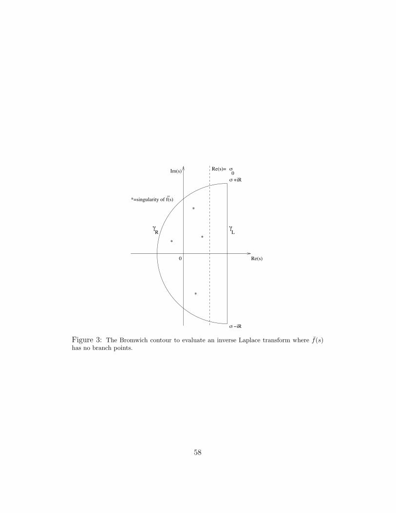
Re(s)
Im(s) Re(s)=
0
!
!!
!
*=singularity of f(s)!
"LR
"
#
# +iR
# !iR
0
Figure 3: The Bromwich contour to evaluate an inverse Laplace transform where f(s)has no branch points.
58
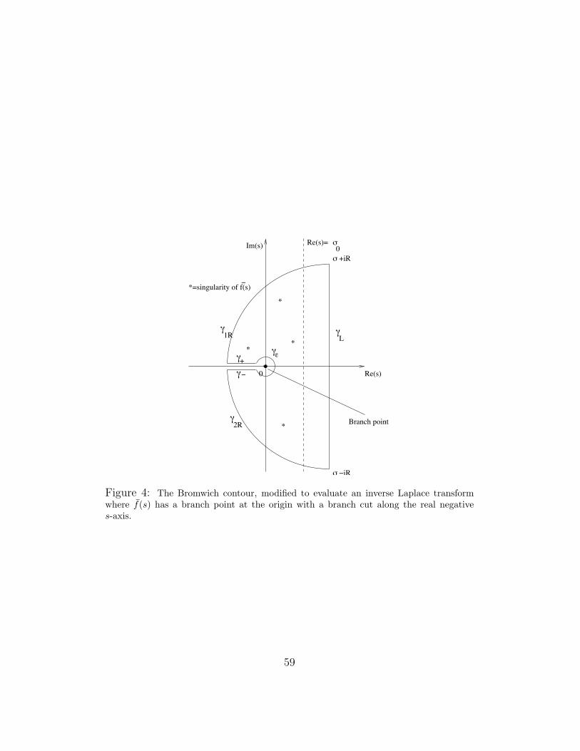
Re(s)
Im(s) Re(s)=
0
!
!!
!
*=singularity of f(s)!
Branch point
"
"+
!
"
"#
"L1R
2R"
$
$ !iR
$ +iR0
Figure 4: The Bromwich contour, modified to evaluate an inverse Laplace transformwhere f(s) has a branch point at the origin with a branch cut along the real negatives-axis.
59
separately. Since f(s) is analytic within the total closed Bromwich contourC we have∮
C
f(s)est ds =
(∫γL
+
∫γ1R
+
∫γ+
+
∫γε
+
∫γ−
+
∫γ2R
)f(s)est ds = 0
and, since the portion we require is the integral along γL, it follows from theInversion theorem that
f(t) =−1
2πi
(∫γ1R
+
∫γ+
+
∫γε
+
∫γ−
+
∫γ2R
)f(s)est ds. (72)
For the integral along γR1 we have s = σ + iReiθ, 0 < θ < π/2, so thatds = −Reiθ dθ, and∣∣∣∣∫
γ1R
f(s)est ds
∣∣∣∣ =
∣∣∣∣∣∫ π/2
0
(σ + iReiθ)−1/2eσte−Rt sin θeiR cos θReiθ dθ
∣∣∣∣∣≤
∫ π/2
0
R−1/2(1 +O(1
R)eσte−Rt sin θRdθ.
Clearly the integrand decays exponentially in R as R → ∞ where θ > 0,so we just have to concern ourselves with whether the contribution from theendpoint θ = 0 decays. Considering the portion 0 < θ < δ for 0 < δ � 1, wehave∫ δ
0
R1/2eσte−Rt sin θ dθ ≈∫ δ
0
R1/2eσte−Rtθ dθ =eσt
t√R
(1− e−Rtδ)→ 0 as R→∞.
[We note, as an aside, that this endpoint contribution would go to zerowhenever the integrand f(s) is of order R−K for some K > 0.] Hence thetotal integral over γ1R goes to zero as R→∞. Similar arguments show thatthe integral over γ2R goes to zero as R→∞.
For the integral along γε we have s = εeiθ, −π < θ < π, so that ds =iεeiθ dθ, and
|f(s) ds| = |(εeiθ)−1/2eεt(cos θ+i sin θ)(iεeiθ) dθ|= ε1/2eεt cos θ dθ.
Hence the integral along this portion goes to zero as ε→ 0.
60
On the curves γ+, γ−, we have s = xeiπ+
, s = xe−iπ−
, respectively, andso (∫
γ+
+
∫γ−
)f(s)est ds =
∫ 0
∞
1
i√xe−xt(−dx) +
∫ ∞0
1
−i√xe−xt(−dx)
= −2i
∫ ∞0
e−xt√xdx.
We evaluate this integral by setting xt = X2, so that dx = 2XdX/t, and(∫γ+
+
∫γ−
)f(s)est ds = − 4i√
t
∫ ∞0
e−X2
dX = −2i
√π
t.
Putting all this together then, from (72) we obtain
f(t) =1√πt.
Homework: Ablowitz & Fokas, problems for section 4.5, questions 13(c),14, 18.
2.3.5 Laplace transform applied to partial differential equations
The properties described in §2.3.3 mean that the Laplace transform (like theFourier transform) can be useful to solve partial differential equations, oftengoverning a quantity that varies both in space and time. For example, thediffusion, or heat, equation
ut = uxx (73)
where t is time and x is position in space governs (among many other things!)the flow of heat in one spatial dimension (e.g. heat flow along a bar). Thisequation is first-order in time and second-order in space, and requires twospatial boundary conditions and an initial condition in time. So forexample we must specify u(a, t), u(b, t) at two known points x = a, x = b,and the initial data u(x, 0). If we take the Laplace transform of (73) withrespect to time t ≥ 0 then with u(x; s) =
∫∞0u(x, t)e−stdt we have
su(x; s)− u(x, 0) =d2u
dx2(x; s), (74)
61
a second order ordinary differential equation for u in x, completed by knowl-edge of the initial condition. The transformed boundary conditions
u(a; s) =
∫ ∞0
u(a, t)e−st dt, u(b; s) =
∫ ∞0
u(b, t)e−st dt,
enable (74) to be solved for u(x; s). Once this is done, inversion needs to beperformed to recover the solution u(x, t) to the original PDE. We considerthis general procedure ((i) transform PDE plus boundary conditions; (ii)solve resulting ODE to obtain Laplace transform of the desired solution; (iii)invert to recover the solution) applied to the following specific example.
Example 2.21 Solve the partial differential equation (a linear wave equa-tion)
utt = uxx, 0 ≤ x ≤ l, t > 0, (75)
with initial conditions
u(x, 0) = 0, ut(x, 0) = sin(πx/l), (76)
and boundary conditions
u(0, t) = 0 = u(l, t). (77)
(Note that as this PDE is second order in time t we require 2 initial condi-tions.)
Laplace-transforming the PDE (75) and boundary conditions (77) in t,using property 3 of the Laplace transform (equation (65)) together with theinitial conditions (76), leads to the ODE problem
s2u(x; s)− su(x, 0)− ut(x, 0) = uxx(x; s)
⇒ uxx(x; s)− s2u(x, s) = − sin(πxl
), u(0; s) = 0 = u(l; s). (78)
The general solution to the ODE (78) is
u(x; s) = A(s)esx +B(s)e−sx +sin(πx/l)
π2/l2 + s2,
and A(s), B(s) must be determined from the boundary conditions, whichyield A(s) = 0 = B(s). We next have to invert u(x; s) = sin(πx/l)/(π2/l2 +
62
s2). We can do this either by using the result of example 2.17, which “byinspection” gives
u(x, t) =1
πsin(πxl
)sin
(πt
l
),
or, more systematically, we can apply the inversion theorem, which tells usthat
u(x, t) =1
2πilimR→∞
∫ σ+iR
σ−iRu(x; s)est dt, t > 0.
The integrand has just two simple poles, at s = ±iπ/l and no branchpoints, hence we evaluate it by applying the Residue theorem to a standardBromwich contour (figure 3) for any real σ > 0.
The semicircular part of the contour γR may be parametrized by s =σ + iReiθ, for 0 ≤ θ ≤ π, so that for this part of the integral we have
IR =
∫γR
u(x; s)est dt =
∫ π
0
−eσte−Rt sin θReiθ dθ
λ2 + (σ + iReiθ)2
=1
R
∫ π
0
eσte−Rt sin θeiRt cos θe−iθ dθ(1− iσ
Re−iθ
)2 − λ2
R2 e−2iθ
⇒ |IR| ≤1
R
∫ π
0
eσte−Rt sin θ dθ∣∣∣∣∣1− σR
∣∣2 − λ2
R2
∣∣∣ → 0 as R→∞.
The total integral around the closed Bromwich contour C is then equal justto the portion along the straight line, γL, which is exactly what we requirefor the Laplace inversion theorem. Thus, applying the Residue theorem wehave
u(x, t) = [Residue of u(x; s)est at iπ/l] + [Residue of u(x; s)estat −iπ/l].
We evaluate the residues using (34) (theorem 2.2), which gives
Res(u(x; s)est;±iπ/l) = lims→±iπ/l
(s∓ iπ/l) sin(πx/l)est
(s+ iπ/l)(s− iπ/l)
= ±sin(πx/l)e±iπt/l
2πi/l
63
so that, adding the residues,
u(x, t) =l
πsin(πxl
)sin
(πt
l
),
as found by inspection.
Example 2.22 (Diffusion equation) Solve
ut = uxx, 0 < x < 1, t ≥ 0, (79)
ux(0, t) = 0, u(1, t) = u1, (80)
u(x, 0) = u0, (81)
where u1, u0 are constants.
We take the Laplace transform as before (using (65) and (64)) to transformthe PDE (79) and initial condition (81) into a second-order ODE for u(x; s),
uxx − su = −u0, (82)
with boundary conditions from transforming those for the PDE (80),
ux(0; s) = 0, u(1; s) =u1
s. (83)
Equation (82) has solution
u(x; s) = A(s)ex√s +B(s)e−x
√s +
u0
s,
and the boundary conditions give
A(s) = B(s) =u1 − u0
s(e√s + e−
√s).
Hence the solution to the original PDE is given by inverting
u(x; s) =(u1 − u0)
s
coshx√s
cosh√s
+u0
s
⇒ u(x, t) = (u1 − u0)L−1
(coshx
√s
s cosh√s
)+ u0L−1
(1
s
). (84)
The function 1/s is easily inverted by inspection (it is the Laplace Transformof 1), but for the other part we need the Inversion theorem. We thus consider
64
the inversion integrand g(s)est = est coshx√s
s cosh√s
, which has a simple pole at s = 0,
and other singularities at the zeros of cosh√s = cos i
√s. Since cosh
√s is
an analytic function with the Taylor series
cosh√s =
∞∑n=0
sn
(2n)!,
it is in fact single-valued on C, and has only simple zeros at the pointssn = −(2n + 1)2π2/4, on the negative real axis, corresponding to simplepoles of the inversion integrand. We therefore consider a standard Bromwichcontour C as in figure 3, and check that the integral around the semicircularportion γR tends to zero as R → ∞. On γR, s = σ + iReiθ, 0 ≤ θ ≤ π, andthe integral IR around γR satisfies, for R sufficiently large,
|IR| =
∣∣∣∣∣∫ π
0
cosh(x(σ + iReiθ)1/2)e(σ+iReiθ)t(−Reiθdθ)(σ + iReiθ) cosh((σ + iReiθ)1/2)
∣∣∣∣∣≤ M0
∫ π
0
∣∣∣∣cosh(x(σ + iReiθ)1/2)
cosh((σ + iReiθ)1/2)
∣∣∣∣ eσt−Rt sin θdθ
= M0
∫ π
0
|G(θ)| dθ.
Splitting the range of integration, for 0 < θ < π/2 we have
|G(θ)| =cosh
(x√R cos
(θ2
+ π4
)(1 +O
(1R
)))
cosh(√
R cos(θ2
+ π4
)(1 +O
(1R
))) eσt−Rt sin θ
=
[e(−2x
√R cos( θ2 +π
4 )(1+O( 1R))) + 1
e(−2√R cos( θ2 +π
4 )(1+O( 1R))) + 1
]e(x√R cos( θ2 +π
4 )(1+O( 1R)))
e(√R cos( θ2 +π
4 )(1+O( 1R)))
eσt−Rt sin θ.
For 0 < θ < π/2, cos( θ2
+ π4) > 0, and so for x > 0 the term in square brackets
is bounded as R→∞ (by M1, say) and we have
|G(θ)| ≤ M1eσt exp
{−Rt sin θ − (1− x)
√R cos
(θ
2+π
4
)(1 +O
(1
R
))
}→ 0 as R→∞.
It follows that, for 0 < x < 1,∫ π/2
0
|G(θ)| dθ → 0 as R→∞.
65
Similar arguments show that∫ π
π/2
|G(θ)| dθ → 0 as R→∞,
and thus IR, the contribution to the Bromwich integral around the semicircleγR, goes to zero as R→∞.
The Residue theorem is therefore directly applicable to recover the inver-sion integral along the straight-line portion γL of the Bromwich contour Cfor a > 0:
1
2πilimR→∞
∫ σ+iR
σ−iRg(x; s)est ds =
∑all poles
Res
(est cosh(x
√s)
s cosh√s
).
For the pole at s = 0 we have (applying (34))
Res
(est cosh(x
√s)
s cosh√s
, s = 0
)= 1.
For the pole at sn = −(2n + 1)2π2/4 we write s = sn + ε, |ε| � 1, and notethat
cosh√s = cos(i
√s) = cos
(π
2(2n+ 1)
(1− 2ε
π2(2n+ 1)2+ · · ·
))= sin
(π2
(2n+ 1))
sin
(ε
π(2n+ 1)
)+ · · · = (−1)nε
π(2n+ 1)+ · · ·
so that
lims→sn
s− sncosh
√s
= (−1)nπ(2n+ 1).
Finally then,
Res
(est cosh(x
√s)
s cosh√s
, sn
)=
4(−1)n+1
π(2n+ 1)cos
(πx(2n+ 1)
2
)exp
(−(2n+ 1)2π2t
4
),
giving the solution to the original PDE, from (84), as
u(x, t) = u1 +4
π(u1 − u0)
∞∑n=1
(−1)n+1
(2n+ 1)cos
(πx(2n+ 1)
2
)exp
(−(2n+ 1)2π2t
4
).
66
Homework: Ablowitz & Fokas, problems for section 4.6, questions 2, 6(b),7.
3 Conformal Mappings
3.1 Motivation
Many problems that arise in physical applied mathematics are free bound-ary problems, in that the domain on which governing equations have to besolved is itself unknown, and has to be determined as part of the solutionprocess. Often, in fact, the shape of the domain is the main information thatis desired. Many problems in fluid dynamics are of this kind, for example,when solving for free surface flows of water, the equations of hydrodynamicshave to be solved on the domain occupied by the water, which (apart fromany rigid containing boundaries) cannot be specified, but will depend on thevarious forces acting on the flowing fluid. Moreover, many fluid flows canbe described in terms of solutions of Laplace’s equation (2), which (in twospace dimensions) we have already seen can be described in terms of analyticfunctions of a complex variable.
The fact that the domain on which equations must be solved is unknowngreatly increases the difficulty of solving the problem. One possible wayaround this extra difficulty, when we are solving a 2D problem for which thereis a complex variable representation for its solutions, is to transform theunknown domain onto some known domain, of simple geometry (for example,the unit disc). This can be accomplished by means of conformal mapping.Conformal mapping can also be very useful even when we know the domainthat we have to solve on. If the domain has a very complicated shape thenit can be difficult to apply boundary conditions and solve the PDE, but ifwe can map this complicated domain onto one of simple geometry then it isoften easy to solve the related PDE in the new complex plane.
We shall see that it is possible to map any simply-connected domain ontoany other via a conformal transformation (the Riemann mapping theo-rem), meaning that, instead of solving a given PDE (for example, Laplace’sequation) on a domain of difficult and/or unknown geometry, one can in-stead solve a related PDE on (e.g.) the unit disc. In the particular caseof Laplace’s equation, the PDE itself is in fact invariant under conformaltransformation, so that one only has to worry about how the boundary con-
67
ditions transform to the new complex plane, and about the details of theconformal mapping required to accomplish the transformation.
We shall begin by discussing the general principles underlying conformalmapping, and then study some specific examples of conformal transforma-tions, before moving onto applications (drawn from fluid dynamics) for whichconformal mapping can be a very useful tool.
3.2 Conformality: general principles
Consider a curve C ∈ C, and let z = f(ζ), where f is some analytic functionof the complex variable ζ = ξ + iη, define a change of variable from thecomplex variable ζ to the complex variable z. Under such a transformationthe curve C in the ζ-plane will be mapped to another curve C ′ in the z-plane;and we shall refer to such transformations as mappings of the complex plane.
Suppose ζ0 is a fixed point on C, and ζ1 = ζ0 +δζ is another nearby pointon C (so that |δζ| � 1). The corresponding points on C ′ are then z0 = f(ζ0),and
z1 = f(ζ1) = f(ζ0 + δζ) = z0 + (δζ)f ′(ζ0) +(δζ)2
2f ′′(ζ0) +O(|δζ|)3, (85)
by Taylor’s theorem 1.25. Suppose now that the derivative f ′(ζ0) 6= 0.
Definition 3.1 If the mapping function f is defined and analytic on a do-main D ⊂ C, and furthermore has nonzero derivative everywhere on D, thenwe say that f is conformal on the domain D.
Then the two image points and the two preimage points are related as follows:
z1 − z0 = (ζ1 − ζ0)f ′(ζ0) +O((ζ1 − ζ0)2). (86)
If we take ζ1 sufficiently close to ζ0 then the curve C is approximately linearbetween the two points, represented by
C = {ζ : ζ = ζ0 + s exp(i arg(ζ1 − ζ0)), s ∈ [0, |ζ1 − ζ0|]},and ζ1 − ζ0 = |ζ1 − ζ0| exp[i(arg(ζ1 − ζ0)].
At z1 we have, by (86),
z1 = z0 + |ζ1 − ζ0||f ′(ζ0)| exp(i[arg(ζ1 − ζ0) + arg(f ′(ζ0))]). (87)
68
Thus locally, a conformal transformation magnifies distances between pointsby a factor |f ′(ζ0)|, and shifts angles by an additive constant arg(f ′(ζ0)). Ifthe original curve is continuous and differentiable then under the conformaltransformation, the image curve will be also.
Definition 3.2 If f ′(ζ0) = 0 at some point ζ0 then the analytic transforma-tion f is not conformal at that point. Such a point ζ0 is called a criticalpoint of the map f .
To see what happens local to a critical point, we must continue the expansion(85) as far as necessary, to the first non-vanishing derivative, say the nth.Then, noting that
(δζ)n = (|δζ|ei arg δζ)n = |δζ|nein arg δζ ,
it follows that locally two neighboring points on the image curve are relatedby
z1 − z0 =(δζ)n
n!f (n)(ζ0) +O(|δζ|n+1)
=|δζ|n
n!|f (n)(ζ0)| exp(i[n arg(δζ) + arg(f (n)(ζ0))]) +O(|δζ|n+1). (88)
Thus here, in addition to angles being shifted through angle arg(f (n)(ζ0)),they are first multiplied by n. Considering a second small line segment, fromζ0 to the point ζ2 in the preimage plane, we obtain a similar relation to (88)for its image point z2. It follows that when two neighboring infinitesimal linesegments of equal length |δζ| are transformed in this way, the angle betweenthem in the transformed plane (given by arg(z2− z0)− arg(z1− z0)) is equalto the angle between the original line segments, multiplied by the factor n.This is because
z1 − z0 =|δζ|n
n!|f (n)(ζ0)| exp(i[n arg(δζ1) + arg(f (n)(ζ0))]) +O(|δζ|n+1),
z2 − z0 =|δζ|n
n!|f (n)(ζ0)| exp(i[n arg(δζ2) + arg(f (n)(ζ0))]) +O(|δζ|n+1),
⇒ arg(z2 − z0)− arg(z1 − z0) = n(arg(δζ2)− arg(δζ1)).
Remark Note that even if the preimage curve in the ζ-plane does not self-intersect, there is nothing to stop self-intersection of the image curve in thez-plane. However, if the analytic mapping function f is also one-to-one, thenthe image curve will not self-intersect.
69
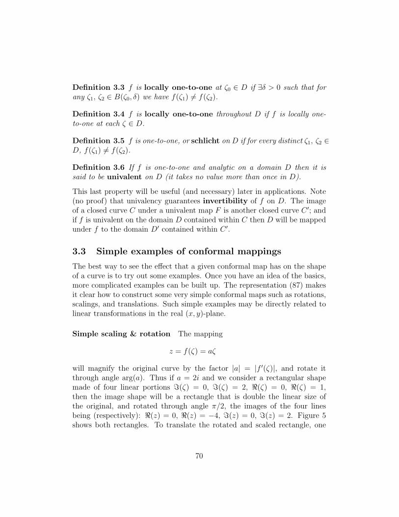
Definition 3.3 f is locally one-to-one at ζ0 ∈ D if ∃δ > 0 such that forany ζ1, ζ2 ∈ B(ζ0, δ) we have f(ζ1) 6= f(ζ2).
Definition 3.4 f is locally one-to-one throughout D if f is locally one-to-one at each ζ ∈ D.
Definition 3.5 f is one-to-one, or schlicht on D if for every distinct ζ1, ζ2 ∈D, f(ζ1) 6= f(ζ2).
Definition 3.6 If f is one-to-one and analytic on a domain D then it issaid to be univalent on D (it takes no value more than once in D).
This last property will be useful (and necessary) later in applications. Note(no proof) that univalency guarantees invertibility of f on D. The imageof a closed curve C under a univalent map F is another closed curve C ′; andif f is univalent on the domain D contained within C then D will be mappedunder f to the domain D′ contained within C ′.
3.3 Simple examples of conformal mappings
The best way to see the effect that a given conformal map has on the shapeof a curve is to try out some examples. Once you have an idea of the basics,more complicated examples can be built up. The representation (87) makesit clear how to construct some very simple conformal maps such as rotations,scalings, and translations. Such simple examples may be directly related tolinear transformations in the real (x, y)-plane.
Simple scaling & rotation The mapping
z = f(ζ) = aζ
will magnify the original curve by the factor |a| = |f ′(ζ)|, and rotate itthrough angle arg(a). Thus if a = 2i and we consider a rectangular shapemade of four linear portions =(ζ) = 0, =(ζ) = 2, <(ζ) = 0, <(ζ) = 1,then the image shape will be a rectangle that is double the linear size ofthe original, and rotated through angle π/2, the images of the four linesbeing (respectively): <(z) = 0, <(z) = −4, =(z) = 0, =(z) = 2. Figure 5shows both rectangles. To translate the rotated and scaled rectangle, one
70
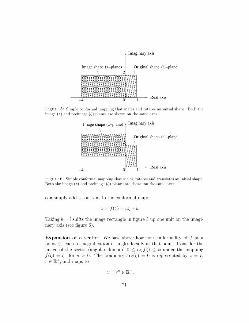
0
Image shape Original shape (!!plane)(z!plane)
Real axis
Imaginary axis
2
1!4
Figure 5: Simple conformal mapping that scales and rotates an initial shape. Both theimage (z) and preimage (ζ) planes are shown on the same axes.
0
Original shape (!!plane)
Real axis
Imaginary axis
2
1!4
Image shape (z!plane)
Figure 6: Simple conformal mapping that scales, rotates and translates an initial shape.Both the image (z) and preimage (ζ) planes are shown on the same axes.
can simply add a constant to the conformal map:
z = f(ζ) = aζ + b.
Taking b = i shifts the image rectangle in figure 5 up one unit on the imagi-nary axis (see figure 6).
Expansion of a sector We saw above how non-conformality of f at apoint ζ0 leads to magnification of angles locally at that point. Consider theimage of the sector (angular domain) 0 ≤ arg(ζ) ≤ φ under the mappingf(ζ) = ζn for n > 0. The boundary arg(ζ) = 0 is represented by z = r,r ∈ R+, and maps to
z = rn ∈ R+,
71
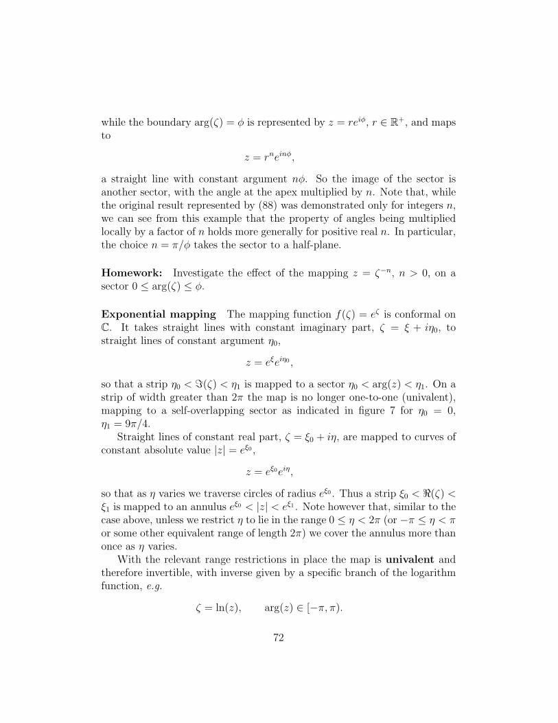
while the boundary arg(ζ) = φ is represented by z = reiφ, r ∈ R+, and mapsto
z = rneinφ,
a straight line with constant argument nφ. So the image of the sector isanother sector, with the angle at the apex multiplied by n. Note that, whilethe original result represented by (88) was demonstrated only for integers n,we can see from this example that the property of angles being multipliedlocally by a factor of n holds more generally for positive real n. In particular,the choice n = π/φ takes the sector to a half-plane.
Homework: Investigate the effect of the mapping z = ζ−n, n > 0, on asector 0 ≤ arg(ζ) ≤ φ.
Exponential mapping The mapping function f(ζ) = eζ is conformal onC. It takes straight lines with constant imaginary part, ζ = ξ + iη0, tostraight lines of constant argument η0,
z = eξeiη0 ,
so that a strip η0 < =(ζ) < η1 is mapped to a sector η0 < arg(z) < η1. On astrip of width greater than 2π the map is no longer one-to-one (univalent),mapping to a self-overlapping sector as indicated in figure 7 for η0 = 0,η1 = 9π/4.
Straight lines of constant real part, ζ = ξ0 + iη, are mapped to curves ofconstant absolute value |z| = eξ0 ,
z = eξ0eiη,
so that as η varies we traverse circles of radius eξ0 . Thus a strip ξ0 < <(ζ) <ξ1 is mapped to an annulus eξ0 < |z| < eξ1 . Note however that, similar to thecase above, unless we restrict η to lie in the range 0 ≤ η < 2π (or −π ≤ η < πor some other equivalent range of length 2π) we cover the annulus more thanonce as η varies.
With the relevant range restrictions in place the map is univalent andtherefore invertible, with inverse given by a specific branch of the logarithmfunction, e.g.
ζ = ln(z), arg(z) ∈ [−π, π).
72
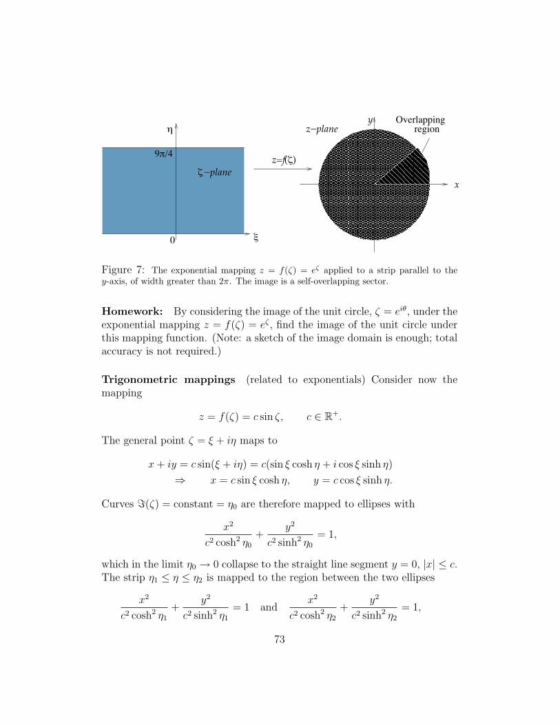
−plane
9!/4
"
0 #
$
y
x
z−planeOverlapping
region
($)z=f
Figure 7: The exponential mapping z = f(ζ) = eζ applied to a strip parallel to they-axis, of width greater than 2π. The image is a self-overlapping sector.
Homework: By considering the image of the unit circle, ζ = eiθ, under theexponential mapping z = f(ζ) = eζ , find the image of the unit circle underthis mapping function. (Note: a sketch of the image domain is enough; totalaccuracy is not required.)
Trigonometric mappings (related to exponentials) Consider now themapping
z = f(ζ) = c sin ζ, c ∈ R+.
The general point ζ = ξ + iη maps to
x+ iy = c sin(ξ + iη) = c(sin ξ cosh η + i cos ξ sinh η)
⇒ x = c sin ξ cosh η, y = c cos ξ sinh η.
Curves =(ζ) = constant = η0 are therefore mapped to ellipses with
x2
c2 cosh2 η0
+y2
c2 sinh2 η0
= 1,
which in the limit η0 → 0 collapse to the straight line segment y = 0, |x| ≤ c.The strip η1 ≤ η ≤ η2 is mapped to the region between the two ellipses
x2
c2 cosh2 η1
+y2
c2 sinh2 η1
= 1 andx2
c2 cosh2 η2
+y2
c2 sinh2 η2
= 1,
73
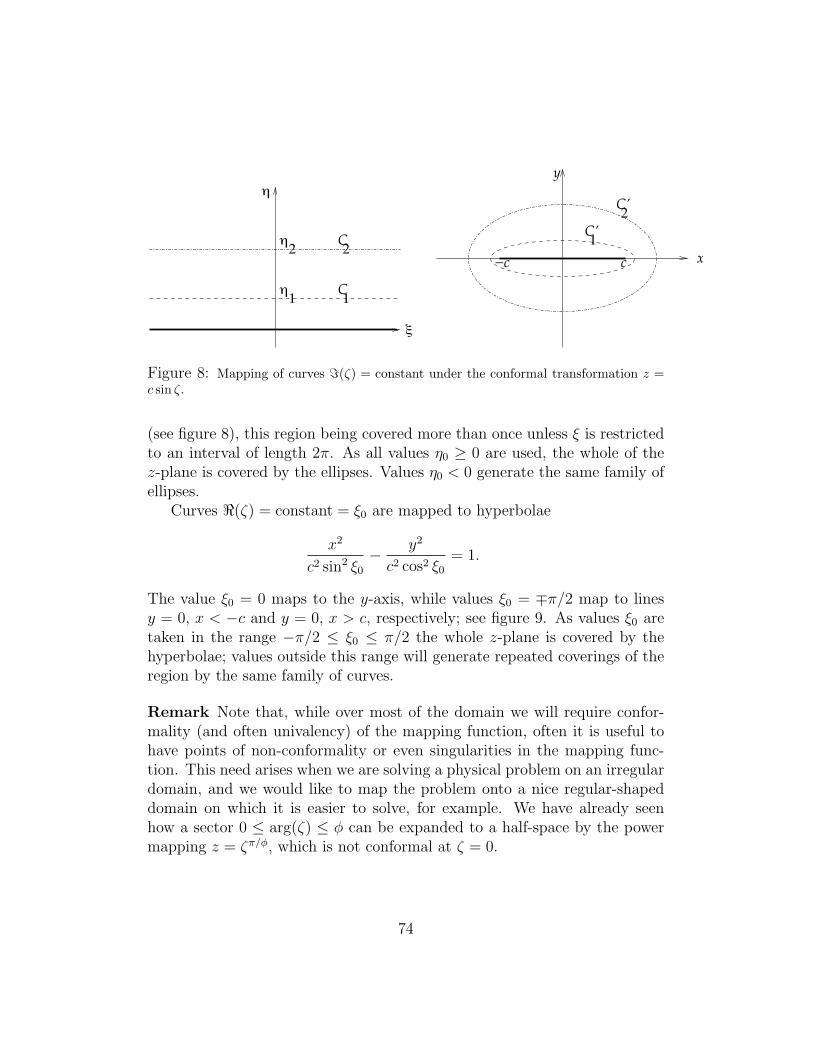
!
!
!
"
x
y
−c cC C’
C
C’
1
2
1
2
2
1
Figure 8: Mapping of curves =(ζ) = constant under the conformal transformation z =c sin ζ.
(see figure 8), this region being covered more than once unless ξ is restrictedto an interval of length 2π. As all values η0 ≥ 0 are used, the whole of thez-plane is covered by the ellipses. Values η0 < 0 generate the same family ofellipses.
Curves <(ζ) = constant = ξ0 are mapped to hyperbolae
x2
c2 sin2 ξ0
− y2
c2 cos2 ξ0
= 1.
The value ξ0 = 0 maps to the y-axis, while values ξ0 = ∓π/2 map to linesy = 0, x < −c and y = 0, x > c, respectively; see figure 9. As values ξ0 aretaken in the range −π/2 ≤ ξ0 ≤ π/2 the whole z-plane is covered by thehyperbolae; values outside this range will generate repeated coverings of theregion by the same family of curves.
Remark Note that, while over most of the domain we will require confor-mality (and often univalency) of the mapping function, often it is useful tohave points of non-conformality or even singularities in the mapping func-tion. This need arises when we are solving a physical problem on an irregulardomain, and we would like to map the problem onto a nice regular-shapeddomain on which it is easier to solve, for example. We have already seenhow a sector 0 ≤ arg(ζ) ≤ φ can be expanded to a half-space by the powermapping z = ζπ/φ, which is not conformal at ζ = 0.
74
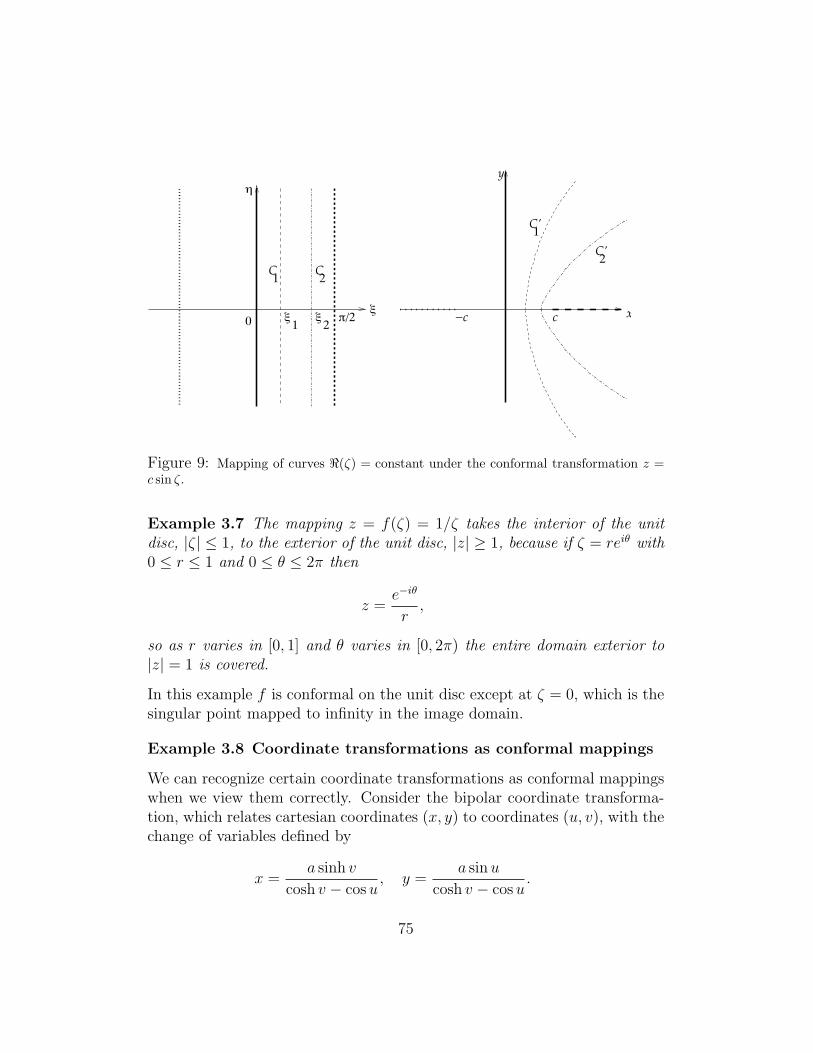
!
"
y
x" "1 20
C2
C1
c−c#/2
C’2
1C’
Figure 9: Mapping of curves <(ζ) = constant under the conformal transformation z =c sin ζ.
Example 3.7 The mapping z = f(ζ) = 1/ζ takes the interior of the unitdisc, |ζ| ≤ 1, to the exterior of the unit disc, |z| ≥ 1, because if ζ = reiθ with0 ≤ r ≤ 1 and 0 ≤ θ ≤ 2π then
z =e−iθ
r,
so as r varies in [0, 1] and θ varies in [0, 2π) the entire domain exterior to|z| = 1 is covered.
In this example f is conformal on the unit disc except at ζ = 0, which is thesingular point mapped to infinity in the image domain.
Example 3.8 Coordinate transformations as conformal mappings
We can recognize certain coordinate transformations as conformal mappingswhen we view them correctly. Consider the bipolar coordinate transforma-tion, which relates cartesian coordinates (x, y) to coordinates (u, v), with thechange of variables defined by
x =a sinh v
cosh v − cosu, y =
a sinu
cosh v − cosu.
75
Coordinate lines u = constant, v = constant each map to circles in the(x, y)-plane, since
x2 + (y − a cotu)2 = a2cosec2u,
which for constant u represent circles with center (0, a cotu) and radiusacosecu. All such circles intersect the x-axis at points x = ±a. Also,
(x− acothv)2 + y2 = a2cosech2v,
which for constant v represent circles with center (acothv, 0) and radiusacosechv < acothv (so for v > 0 all such circles are in the right half-planex > 0 and vice-versa for v < 0).
It is far from obvious that this transformation is equivalent to a conformalmapping, but if we form z = x+ iy, we can show that
z = x+ iy =a(sinh v + i sinu)
cosh v − cosu= ia cot
(ζ
2
),
where ζ = u+ iv.This is most easily demonstrated by showing that the final equality above
holds. With ζ = u+ iv,
ia cot
(ζ
2
)= ia
cos 12(u+ iv)
sin 12(u+ iv)
= iacos u
2cosh v
2− i sin u
2sinh v
2
sin u2
cosh v2
+ i cos u2
sinh v2
= ia(cos u
2cosh v
2− i sin u
2sinh v
2)(sin u
2cosh v
2− i cos u
2sinh v
2)
sin2 u2
cosh2 v2
+ cos2 u2
sinh2 v2
= ia(1
2sinu cosh2 v
2− 1
2sinu sinh2 v
2− i
2sinh v cos2 u
2− i
2sinh v sin2 u
2)
cosh2 v2(1− cos2 u
2) + cos2 u
2(cosh2 v
2− 1)
=ia
2
sinu− i sinh v
cosh2 v2− cos2 u
2
= iasinu− i sinh v
(2 cosh2 v2− 1)− (2 cos2 u
2− 1)
= a(sinh v + i sinu)
cosh v − cosu.
76
Hence the result is proved.
If we are prepared to put up with a nonlinear rescaling of distance, thenstandard polar coordinates could be thought of in a similar manner, as acomplex transformation ζ = log z (conformal away from the origin, with anappropriate branch-cut). The real part of ζ is log |z| = log r, rather than thenormal polar distance r; while =(ζ) is the standard polar angle θ.
Sometimes before attempting a conformal transformation between twogiven domains, it can help to spend some time thinking of the most ap-propriate geometrical description of the regions, as the following exampleillustrates.
Example 3.9 Find a mapping from the interior of the unit disc to the upper-half z-plane.
Such a map necessarily has a point of non-analyticity, since we are trans-forming from a finite domain to an infinite one. In this case an easy way tofind the desired transformation is to note that the defining characteristic ofthe unit disc is that it is the set of points ζ ∈ C such that |ζ| ≤ 1, while aconvenient way to define the upper half-plane is that it is exactly the set ofpoints z ∈ C that are closer to i than −i, and therefore |z − i| < |z + i|. Itfollows that the map
ζ =z − iz + i
takes the upper-half z-plane onto the unit disc |ζ| ≤ 1. We are asked for theinverse of this map, so we simply rearrange the above relation to find that
z = f(ζ) =i(1 + ζ)
(1− ζ)(89)
is a mapping function that will do the trick.3 This map is singular at thepoint ζ = 1 on the boundary of the unit disc; this is the point that is mappedto ∞ on the “boundary” of the upper half plane.
3It is not the only one that would work; for example we could first rotate the unit discthrough any arbitrary angle before applying the above transformation to the rotated disc.We will say more later about conditions that guarantee uniquenss of a conformal mapbetween given domains.
77
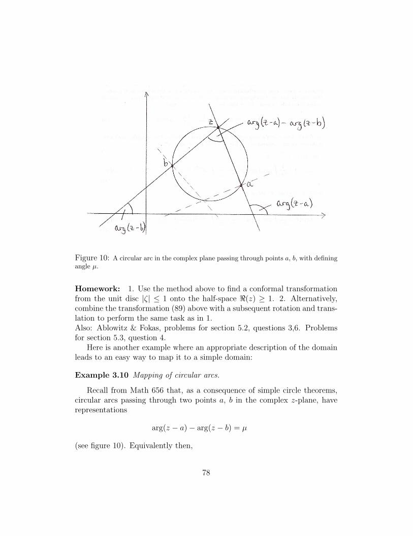
Figure 10: A circular arc in the complex plane passing through points a, b, with definingangle µ.
Homework: 1. Use the method above to find a conformal transformationfrom the unit disc |ζ| ≤ 1 onto the half-space <(z) ≥ 1. 2. Alternatively,combine the transformation (89) above with a subsequent rotation and trans-lation to perform the same task as in 1.Also: Ablowitz & Fokas, problems for section 5.2, questions 3,6. Problemsfor section 5.3, question 4.
Here is another example where an appropriate description of the domainleads to an easy way to map it to a simple domain:
Example 3.10 Mapping of circular arcs.
Recall from Math 656 that, as a consequence of simple circle theorems,circular arcs passing through two points a, b in the complex z-plane, haverepresentations
arg(z − a)− arg(z − b) = µ
(see figure 10). Equivalently then,
78
arg
(z − az − b
)= µ.
This remarkably simple observation gives us an easy way to transform circulararcs into straight lines through the origin! More remarkably, the crescent-or lens-shaped region between two circular arcs that intersect at points a, b,can be transformed into a sector, simply by applying the transformation
w =z − az − b
.
If the first arc has defining angle µ1 and the second µ2 > µ1, then the regionbetween them will be transformed into the sector
µ1 < arg(w) < µ2.
The point z = a maps to the origin in the w-plane, while w = b maps toinfinity.
3.4 Detour: Laplace’s equation under conformal trans-formation
Many physical problems of interest (problems in inviscid fluid flow, poten-tial theory problems in electrostatics and gravitation, and many more) aregoverned by Laplace’s equation on a given domain D′
∂2u
∂x2+∂2u
∂y2= 0, for (x, y) ∈ D′, (90)
subject to appropriate boundary conditions on the boundary of the domain,∂D (for example, the values of u on ∂D′ may be specified). If the boundaryof D′ has an irregular shape then (90) can be very difficult to solve; howeverthere are known techniques (e.g. Green’s functions, separation of variables)for solving Laplace’s equation on canonical “nice” domains such as the unitcircle or a half-space. Suppose we are able to map conformally from such a“nice” domain D (say the unit disc, to be specific) in the ζ-plane, onto theirregular domain D′ in the z-plane via z = f(ζ).
By Lemma 1.8 u must be the real part of an analytic function, u(x, y) =<(g(z)) on D′. We can then define an analytic function G(ζ) on D via
G(ζ) = g(f(ζ)) ≡ (g ◦ f)(ζ),
79
(the composition of two analytic functions is another analytic function) andif U(ξ, η) = <(G(ζ)) then U is a harmonic function of (ξ, η), and at corre-sponding points in the two complex planes we have
U(ξ, η) = <(G(ζ)) = <(g(f(ζ))) = <(g(z)) = u(x, y).
Thus, if we know the values of U(ξ, η) (which we find by solving Laplace’sequation on the “nice” domain), and the conformal map f that takes points(ξ, η) to points (x, y), then we have solved the original problem for u(x, y).We have already mentioned that it is known how to solve Laplace’s equationwith given boundary data on nice canonical domains, therefore the crucialpart of the above procedure is whether the desired conformal mapping canbe found. That it can is guaranteed by the following theorem, which we statefirst informally:
Theorem 3.11 (Riemann mapping theorem — informal statement) Anytwo simply-connected domains, each having more than one boundary point,can be mapped conformally one on the other.
Unfortunately, neither the theorem, nor its proof, give any hint as tohow one might construct the desired mapping in a given situation. However,there is an important special case in which one can construct a conformalmapping explicitly: when one is mapping from a simple canonical domain(such as a half-space or the unit disc) onto the interior of an arbitrary poly-gon. The associated conformal mapping is called the Schwarz-Christoffeltransformation, and is outlined in Appendix A.
3.5 Riemann mapping theorem
Definition 3.12 (Conformal equivalence) We call two regions D and D′
conformally equivalent if there exists a function f univalent on D suchthat D′ = f(D), that is, if there exists a conformal one-to-one mapping ofD′ onto D.
An equivalent statement of the Riemann mapping theorem is:
Theorem 3.13 (Riemann mapping theorem) Every simply-connected regionD in the plane is conformally equivalent to the unit disc.
80
The mapping of any one region to any other is not unique. In order toexplore the freedom in the mapping it is instructive first to consider howmany different ways the unit disc may be mapped to itself.
Definition 3.14 A one-to-one conformal mapping of any region to itself iscalled an automorphism of the region.
As a preliminary to proving results about general automorphisms of the unitdisk, we first state and prove:
Lemma 3.15 (Schwarz Lemma) Let f : B(0, 1)→ B(0, 1) be analytic, withf(0) = 0. Then |f ′(0)| ≤ 1 and |f(z)| ≤ |z| ∀z ∈ B(0, 1). If |f ′(0)| = 1 or|f(z)| = |z| for some z ∈ B(0, 1)\{0} then f(z) = eiαz for some α ∈ R.
Proof Since f(0) = 0 the function defined by
g(z) =
{f(z)
zz 6= 0,
f ′(0) z = 0,
is analytic in B(0, 1) (a simple consequence of Taylor’s theorem 25). Weclaim that |g(z)| ≤ 1 for all z ∈ B(0, 1). For, suppose that |g(z∗)| = t > 1for some z∗ ∈ B(0, 1), |z∗| < 1. Let rn = 1− 1/n, then for rn > |z∗| (that is,n > 1/(1 − |z∗|)) the maximum modulus principle applied to g on B(0, rn)states that the maximum of |g| must occur on the boundary, |z| = rn. Sincewe know |g(z∗)| = t and z∗ ∈ B(0, rn), we therefore have some point zn with|zn| = rn and |g(zn)| ≥ t. But since t > 1 is fixed and rn can be madearbitrarily close to 1, we can also choose n large enough that rnt > 1 andthen
|g(zn)| ≥ t ⇒ |f(zn)| ≥ t|zn| = trn > 1,
which contradicts the assumption that f : B(0, 1)→ B(0, 1).This proves the claim that |g(z)| ≤ 1 for all z ∈ B(0, 1), and there are now
two possibilities. Either g is a constant of modulus 1 or, by the maximummodulus theorem 1.10, we have |g(z)| < 1 for all z ∈ B(0, 1). If |f ′(0)| = 1or |f(z)| = |z| for some z ∈ B(0, 1)\{0} then the latter possibility cannothold, and so g(z) = eiα for some α ∈ R, giving f(z) = eiαz.
Lemma 3.16 (Automorphisms of the unit disc that fix the origin) The onlyautomorphisms of the unit disc with f(0) = 0 are given by f(ζ) = eiαζ, someα ∈ R.
81
Proof Write ζ1 = f(ζ) for the mapping from the unit disc in the ζ-plane tothe unit disc in the ζ1-plane. By the Schwarz lemma 3.15, |ζ1| = |f(ζ)| ≤ |ζ|for |ζ| < 1. Since f is 1-1 it is also invertible; and ζ = f−1(ζ1) is anotherautomorphism of the unit disc with f−1(0) = 0, so also |ζ| = |f−1(ζ1)| ≤ |ζ1|.It follows that |ζ1| = |ζ|, or |f(ζ)| = |ζ|, and thus f(ζ) = eiαζ.
Lemma 3.17 (Automorphisms of the unit disc) The automorphisms of the
unit disc are of the form f(ζ) = eiα(ζ−a1−aζ
), where α ∈ R and |a| < 1.
Proof Any automorphism of the unit disc must map some point a ∈ B(0, 1)to the origin. Let w = g(ζ) = ζ−a
1−aζ . Then g is analytic and single-valued on
the unit disc, and the point ζ = a within B(0, 1) maps to w = 0 ∈ B(0, 1).Also,
|w|2 =|ζ|2 − aζ − aζ + |a|2
1− aζ − aζ + |a|2|ζ|2= 1, for |ζ| = 1.
By the maximum modulus theorem 1.10 it follows that |g(ζ)| ≤ 1, and g is amapping from B(0, 1) to B(0, 1). The function g is also 1-1 from B(0, 1) toitself, since
w = g(ζ) ⇒ ζ =w + a
1 + aw= g−1(w)
(a function of exactly the same type as g), which shows that to any imagepoint |w| ≤ 1 there corresponds a preimage point ζ ∈ B(0, 1) (exactly thesame argument as for g proves that |g−1(w)| ≤ 1 for w ∈ B(0, 1)). Thereforeg is a 1-1 mapping of the unit disc to itself, that is, an automorphism.
Suppose now that f is another automorphism of the unit disc such thatf(a) = 0. Then h = f ◦ g−1 is another automorphism of B(0, 1), and h(0) =f(g−1(0)) = f(a) = 0. By lemma 3.16 above then, h(ζ) = eiαζ; and withw = g(ζ), ζ = g−1(w) we have
h(w) = (f ◦ g−1)(w) ⇒ f(ζ) = h(g(ζ)) = eiαg(ζ) = eiα(ζ − a1− aζ
).
Lemma 3.18 (Uniqueness of mappings between domains) Suppose D1 andD2 are simply-connected domains, that f : D1 → D2 is a 1-1 conformalmapping between them, and that g is an automorphism of D2. Then(a) Any other 1-1 conformal mapping F : D1 → D2 is of the form g ◦ f .(b) Any automorphism h of D1 is of the form f−1 ◦ g ◦ f .
82
Proof (a) If f and F are both 1-1 conformal mappings of D1 onto D2, thenF ◦ f−1 is an automorphism g of D2, that is, F ◦ f−1 = g, so that F = g ◦ f .(b) If h is an automorphism of D1 then f ◦ h ◦ f−1 is an automorphism ofD2, since (applying the maps in sequence) f−1 is a 1-1 mapping of D2 toD1, h is an automorphism of D1, and f is a 1-1 mapping of D1 to D2. So,f ◦ h ◦ f−1 = g, and thus h = f−1 ◦ g ◦ f .
Homework: On the following theorem.
Theorem 3.19 (Automorphisms of the upper half-plane) The automorphismsof the upper half-plane D+ are of the form
f(ζ) =aζ + b
cζ + d, (91)
with a, b, c, d ∈ R, and ad− bc > 0.
To do: You should first verify that f maps D+ to D+ by showing thatthe boundary maps to the boundary and that an interior point maps to aninterior point. Next check for the one-to-one (invertible) nature of the map.Then use the result of example 3.9 together with lemmas 3.18 and 3.17 toprove the theorem.
Remark The mapping (91) is known as a Mobius transformation orbilinear mapping, and will be studied in generality in §3.7.
Theorem 3.20 (Uniqueness of map in Riemann mapping theorem) Theconformal mapping f from |ζ| ≤ 1 onto the simply connected region D isuniquely specified by any of the following:
1. Specifying the image z0 of ζ = 0 under f , and specifying f ′(0) ∈ R+;or
2. Specifying the image z0 of ζ = 0 under f , and specifying that ζ1 on|ζ| = 1 maps to a given point z1 on ∂D; or
3. Choosing three arbitrary points ζ1, ζ2, ζ3 on |ζ| = 1 and specifying thethree image points z1, z2, z3 on ∂D (the two sets of points appearing inthe same order as the boundary is traversed in the same sense).
83
Proof (of uniqueness)
1. Let f1, f2 be two mappings with property 1, then F = f−11 ◦ f2 is an
automorphism of B(0, 1). Also,
F (0) = f−11 (f2(0)) = f−1
1 (z0) = 0,
so by lemma 3.16 F (ζ) = eiαζ, where α ∈ R. But then
eiα = F ′(ζ) =d
dζ
(f−1
1 (f2(ζ)))
= f−1′
1 (f2(ζ))f ′2(ζ)
⇒ eiα = F ′(0) = f−1′
1 (z0)f ′2(0) =f ′2(0)
f ′1(0)∈ R+,
where in the last line we used the fact that f−1′ = 1/f ′.Exercise: Prove this last result.It follows that α = 0 (modulo 2π), and thus that F (ζ) = ζ, and f2 = f1.
2. Again let f1, f2 be two mappings with property 2, then as above F =f−1
1 ◦ f2 = eiαζ. Also,
eiαζ1 = F (ζ1) = f−11 (f2(ζ1)) = f−1
1 (z1) = ζ1,
thus again, α = 0 (modulo 2π), and f2 = f1.
3. As above, F = f−11 ◦f2 is an automorphism of B(0, 1), and so by lemma
3.17,
F (ζ) = eiαζ − a1− aζ
,
and F has three distinct fixed points ζ1, ζ2, ζ3. But any fixed point ζ∗of F satisfies
aζ2∗ + ζ∗(e
iα − 1)− aeiα = 0,
a quadratic equation with at most two distinct roots, unless a = 0 andα = 0 (modulo 2π). The result f1 = f2 again follows.
Homework: Read up on the proof of the Riemann mapping theorem (non-examinable).
84
3.6 Joukowski transformation
One mapping transformation that is very important in inviscid flow applica-tions (in particular, aerodynamics) is the Joukowski transformation, definedby
z = f(ζ) = ζ +a2
ζ, a ∈ R+. (92)
Noting that f ′(ζ) = 1 − a2/ζ2, the map is conformal except at the pointsζ = 0, ζ = ±a. Circles |ζ| = r transform via
z = x+ iy =
(r +
a2
r
)cos θ + i
(r − a2
r
)sin θ
hence the circle |ζ| = r > a is mapped to the ellipse
x2
(r + a2/r)2+
y2
(r − a2/r)2= 1,
and the region exterior to the circle |ζ| = r > a is mapped to the regionexterior to this ellipse.
The circle of radius a is a special case, containing 2 points of non-conformality, and maps to the slit |x| ≤ 2a, y = 0.
Consider next what happens to circles not centered on the origin under(92); in particular, what happens to a circle that passes through just one ofthe points of non-conformality. Such a circle is given by
|ζ − δ| = a+ δ, δ > 0,
which passes through ζ = −a. Clearly the resulting shape will be smoothexcept for a sharp point at the image of ζ = −a; and for 0 < δ � 1 (wherewe anticipate a slender shape close to the straight line segment |x| ≤ 2a) wecan set ζ = δ + (a+ δ)eiθ and expand in powers of δ to find an approximateexpression for the image shape in terms of the parameter θ:
z = x+ iy = 2a cos θ + 2δ sin θ(sin θ + i(1 + cos θ)) +O(δ2)
⇒{x = 2a cos θ + 2δ sin2 θ +O(δ2)y = 2δ sin θ cos2(θ/2) +O(δ2).
(93)
85
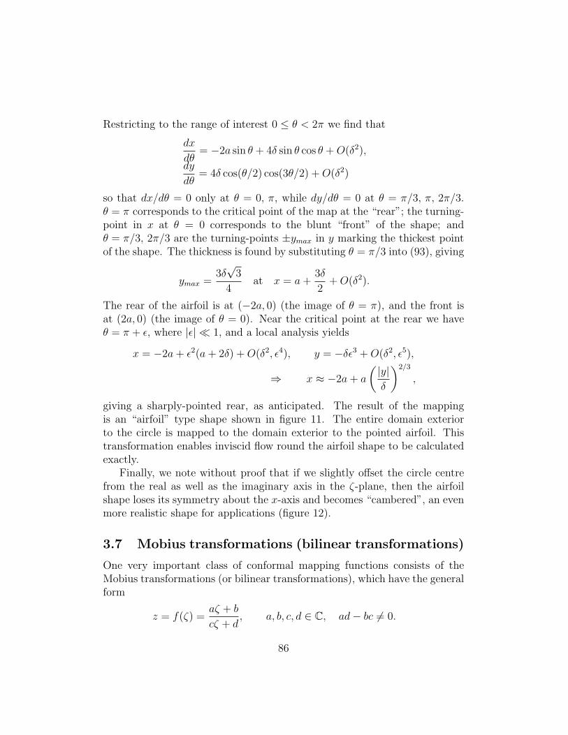
Restricting to the range of interest 0 ≤ θ < 2π we find that
dx
dθ= −2a sin θ + 4δ sin θ cos θ +O(δ2),
dy
dθ= 4δ cos(θ/2) cos(3θ/2) +O(δ2)
so that dx/dθ = 0 only at θ = 0, π, while dy/dθ = 0 at θ = π/3, π, 2π/3.θ = π corresponds to the critical point of the map at the “rear”; the turning-point in x at θ = 0 corresponds to the blunt “front” of the shape; andθ = π/3, 2π/3 are the turning-points ±ymax in y marking the thickest pointof the shape. The thickness is found by substituting θ = π/3 into (93), giving
ymax =3δ√
3
4at x = a+
3δ
2+O(δ2).
The rear of the airfoil is at (−2a, 0) (the image of θ = π), and the front isat (2a, 0) (the image of θ = 0). Near the critical point at the rear we haveθ = π + ε, where |ε| � 1, and a local analysis yields
x = −2a+ ε2(a+ 2δ) +O(δ2, ε4), y = −δε3 +O(δ2, ε5),
⇒ x ≈ −2a+ a
(|y|δ
)2/3
,
giving a sharply-pointed rear, as anticipated. The result of the mappingis an “airfoil” type shape shown in figure 11. The entire domain exteriorto the circle is mapped to the domain exterior to the pointed airfoil. Thistransformation enables inviscid flow round the airfoil shape to be calculatedexactly.
Finally, we note without proof that if we slightly offset the circle centrefrom the real as well as the imaginary axis in the ζ-plane, then the airfoilshape loses its symmetry about the x-axis and becomes “cambered”, an evenmore realistic shape for applications (figure 12).
3.7 Mobius transformations (bilinear transformations)
One very important class of conformal mapping functions consists of theMobius transformations (or bilinear transformations), which have the generalform
z = f(ζ) =aζ + b
cζ + d, a, b, c, d ∈ C, ad− bc 6= 0.
86
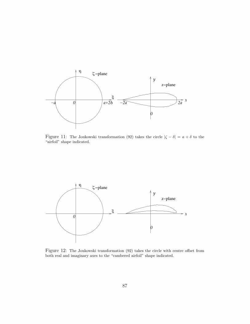
0
0
!
−a −2a 2a x
yz!plane
!plane"
a+2#$
Figure 11: The Joukowski transformation (92) takes the circle |ζ − δ| = a + δ to the“airfoil” shape indicated.
0
0
!
x
yz!plane
!plane"
#
Figure 12: The Joukowski transformation (92) takes the circle with centre offset fromboth real and imaginary axes to the “cambered airfoil” shape indicated.
87
We have already come across such mappings in examples 3.7 and 3.9 (wherewe mapped the interior of a circle to the exterior of a circle, and the interiorof a circle to a half-plane), and in theorem 3.19. We shall see below that, ifwe consider a straight line as being the limiting form of a circle, then Mobiustransformations always map circles to circles.
Section 5.7 in Ablowitz & Fokas gives a very detailed overview of Mobiustransformations; here we summarize the important points for our purposes.
1. Mobius transformations are conformal away from ζ = −d/c (the solepoint where the map is nonanalytic), since
f ′(ζ) =ad− bc
(cζ + d)2
and ad− bc 6= 0.
2. Mobius transformations may be decomposed into the three simplertransformations
w = f1(ζ) = cζ + d, u = f2(w) =1
w,
z = f3(u) =a
c+
(bc− ad)
cu, (94)
so that
z = f(ζ) = f3(f2(f1(ζ))) = (f3 ◦ f2 ◦ f1)(ζ).
f1 and f3 represent a combination of scaling/rotation and translation(as we saw earlier), while f2 represents inversion in the unit circle (thistransformation takes the interior of the unit circle to its exterior).
3. Mobius transformations are one-to-one, and therefore invertible, if weinclude the point infinity in each of the complex ζ- and z planes. With
z = f(ζ) =aζ + b
cζ + d
we have
ζ = f−1(z) =−dz + b
cz − a.
Thus the inverse transformation is another Mobius transformation.
88
4. Mobius transformations have at most two fixed points. Suppose ζ0 =f(ζ0), then
ζ0(cζ0 + d) = aζ0 + b ⇒ cζ20 + (d− a)ζ0 − b = 0.
Since this is a quadratic equation it has at most two roots, or just onein the exceptional case (d− a)2 + 4bc = 0.
5. Theorem 3.21 A bilinear transformation is uniquely determined byspecification of three distinct preimage points in the ζ-plane, and thecorresponding (distinct) image points in the z-plane.
The proof we will give uses the following
Lemma 3.22 The cross-ratio of four preimage points ζj, and four cor-responding image points zj (j = 1, 2, 3, 4) is an invariant, that is,
(z1 − z4)(z3 − z2)
(z1 − z2)(z3 − z4)=
(ζ1 − ζ4)(ζ3 − ζ2)
(ζ1 − ζ2)(ζ3 − ζ4). (95)
Proof (Lemma) Define the cross-ratio function X(ζ1, ζ2, ζ3, ζ4) to bethe right-hand side of (95). Since we know the bilinear transforma-tion can be decomposed into linear transformations and inversions, asin (94), it is enough to show that these sub-transformations leave Xunchanged.
Considering the sub-transformation w = f1(ζ) in (94), we have
(w1 − w4)(w3 − w2)
(w1 − w2)(w3 − w4)=c(ζ1 − ζ4)c(ζ3 − ζ2)
c(ζ1 − ζ2)c(ζ3 − ζ4)=
(ζ1 − ζ4)(ζ3 − ζ2)
(ζ1 − ζ2)(ζ3 − ζ4).
Under the second sub-transformation (inversion) f2 we have
(u1 − u4)(u3 − u2)
(u1 − u2)(u3 − u4)=
(1/w1 − 1/w4)(1/w3 − 1/w2)
(1/w1 − 1/w2)(1/w3 − 1/w4)× w1w2w3w4
w1w2w3w4
=(w4 − w1)(w2 − w3)
(w2 − w1)(w4 − w3),
which is exactly the cross-ratio of the four points wj j = 1, 2, 3, 4.
The third sub-transformation f3 in (94) is again linear, so the resultholds as for f1. Hence the lemma is proved.
89
Proof (Theorem 3.21) Replace ζ4 by ζ and z4 by z, then (95) definesa bilinear transformation z = f(ζ) that takes distinct points ζ1, ζ2,ζ3 to z1, z2, z3. Suppose there exists another such bilinear transfor-mation F 6= f taking ζ1, ζ2, ζ3 to z1, z2, z3, then since F and f aredifferent transformations ∃ ζ4 ∈ C such that Z4 = F (ζ4) 6= z4 = f(ζ4).But by invariance of the cross-ratio of four points (95) for each of thetransformations F and f , we must have
(z1 − z4)(z3 − z2)
(z1 − z2)(z3 − z4)=
(z1 − Z4)(z3 − z2)
(z1 − z2)(z3 − Z4)
⇒ Z4(z1 − z3) = z4(z1 − z3) ⇒ Z4 = z4,
since the points are all distinct. This contradicts the assumption, andthe bilinear transformation is unique, as claimed.
Corollary 3.23 The unique bilinear mapping sending ζ1, ζ2, ζ3 to thepoints 0, ∞, 1 (respectively), is given by
z = f(ζ) =(ζ − ζ1)(ζ3 − ζ2)
(ζ − ζ2)(ζ3 − ζ1). (96)
Proof It is clear that (96) is a bilinear mapping that takes ζ1, ζ2, ζ3
to the points 0, ∞, 1 (respectively). Uniqueness follows from theorem3.21.
Remark To construct the mapping given in the proof above, note thatsetting z1 = 0, z2 =∞, z3 = 1, z4 = z and ζ4 = ζ in (95) gives
−z1− z
=(ζ1 − ζ)(ζ3 − ζ2)
(ζ1 − ζ2)(ζ3 − ζ),
which rearranges trivially to (96).
Returning to example 3.9, we now recognise it as the unique Mobiustransformation taking the points ζ1 = −1, ζ2 = 1 and ζ3 = −i (all ofwhich lie on the unit circle) to the points 0, ∞ and 1, respectively.
6. Mobius transformations map circles (or lines) into circles (or lines).Proof: To show this, it is enough to show that each of the three sub-transformations f1, f2, f3 in (94) map circles or lines to circles or lines.
90
First, suppose that C is a circle, with center at α ∈ C and radius r > 0.The equation in the ζ-plane is
|ζ − α| = r ⇒ ζ = α + reiθ, θ ∈ [0, 2π),
and if c = |c|ei arg(c) then a general point on the image curve under f1
is
w = f1(ζ) = αc+ d+ |c|rei(θ+arg(c))
which lies on the circle with center αc + d and radius r|c|. If C is astraight line then it can be represented in the ζ-plane by equation4
<(βζ) = γ, for β ∈ C, γ ∈ R.
Since ζ = (w − d)/c the equation in the w-plane is
<(β
c(w − d)
)= γ ⇒ <
(βw
c
)= γ + <
(βd
c
),
so that if <(βd/c) 6= −γ then
<(
βw
c(γ + <(βd/c))
)= 1,
which is the equation of a straight line; while if <(βd/c) = −γ then<(βw/c) = 0, also the equation of a straight line.
If C is the same circle in the w-plane then
|w − α|2 = r2 ⇒ ww − αw − αw + |α|2 = r2. (97)
To find the image in the u-plane we note that w = 1/u and thusprovided the circle does not pass through the origin (so that |α| 6= r)we have
1
uu− α
u− α
u+ |α|2 = r2 (98)
⇒ uu+αu
r2 − |α|2+
αu
r2 − |α|2=
1
r2 − |α|2.
4If β = β1 + iβ2 and ζ = ξ + iη then <(βζ) = γ is equivalent to β1ξ − β2η = γ.
91
Comparing with the form of equation (97) we see that u lies on a circlewith center A and radius R given by
A =α
|α|2 − r2, R =
r
||α|2 − r2|
respectively. If the circle does pass through the origin, |α| = r, andequation (98) for u is simpler:
2<(αu) = 1 ⇒ 2(α1u1 − α2u2) = 1,
if α = α1 + iα2 and u = u1 + iu2. This is clearly the equation of astraight line in the u-plane.
To check that straight lines map to straight lines or circles under f2 letC be the straight line
<(βw) = γ
in the w-plane. Then, since w = 1/u, <(β/u) = γ and hence
β1u1 + β2u2
u21 + u2
2
= γ ⇒(u1 −
β1
2γ
)2
+
(u2 −
β2
2γ
)2
=β2
1 + β22
4γ2,
the equation of a circle in the u-plane (a straight line if γ = 0).
Finally, if C is the circle or straight line in the u-plane then, since f3 isa simple linear map like f1, we have already shown that the image ofC in the z-plane is another circle or straight line.
Homework A circle or straight line in C divides the complex plane intotwo complementary regions, one on either side of the boundary (for acircle the two regions are the circle interior and exterior; for a line we havethe two half-spaces on either side of the line). Show that a Mobius trans-formation takes the complementary regions of the preimage circle or line tothe complementary regions of the image circle or line. [Hint: Consider theimages of the complementary regions under the sub-transformations (94).]Also: Ablowitz & Fokas, problems for section 5.7, question 1,
92
3.8 Composition of conformal maps
In order to map a given domain onto another desired domain, it is oftenconvenient to use a series of conformal mappings to intermediate domains,and compose all the maps at the end to obtain the final transformation.
Example 3.24 Find a conformal mapping from the strip 0 < =(ζ) < 1 tothe circle |z − a| = b.
There are many ways of approaching this problem, but we choose to map viaan intermediate domain that we choose to be the upper half plane. We knowthat we can map the strip onto sectors (and the upper half plane is a specialcase of a sector) via an exponential mapping function, and the corollary 3.23above then gives us a constructive method to map the half-space onto theinterior of the given circle.
The mapping u = eαζ takes the strip 0 < =(ζ) < 1 to the sector 0 <arg u < α, so choosing α = π takes the strip to the upper half u-plane.
We then want to find a Mobius transformation between the upper halfu-plane and the disc |z − a| < b. By (96), the mapping
u =(1− i)(z − (a− b))
2(z − (a+ ib))
takes the points z1 = a−b, z2 = a+ib, z3 = a+b to u = 0, ∞, 1, respectively.Inverting this map gives
z =2u(a+ ib)− (1− i)(a− b)
2u− (1− i),
so that the final mapping desired is given by the composition,
z =2eπζ(a+ ib)− (1− i)(a− b)
2eπζ − (1− i).
Remark As a final check it is always a good idea to ensure that an interiorpoint in the preimage domain maps to one in the image domain. The pointz = a within the circle corresponds to u = (1 + i)/2 in the upper half-plane, and this in turn corresponds to the point ζ = − log |
√2| + iπ/4,
which does indeed lie in the appropriate strip. When mapping boundariesto boundaries, there is always the possibility that one is mapping to theexterior of the desired domain. With the constructive method presented
93
for Mobius transformations, a useful rule to remember is that the sense ofthe domain will be preserved under the mapping. Thus, in the mapping z(u)above, marching along the boundary from u1 = 0 to u3 = 1 to u2 = ∞, wekeep the domain (the upper half-plane) to our left. This is also the case inthe z-plane, hence the image points, z1 = a − b, z3 = a + b, z2 = a + ib aregood choices, because moving from z1 to z3 to z2 takes us around the circleanticlockwise, keeping its interior to the left. Thus, the circle’s interior willbe the image domain of the upper half plane.
Homework: Ablowitz & Fokas, problems for section 5.7, questions 2,3,6.
4 Applications of conformal mapping
Many of the common applications of conformal mapping and other complexvariable techniques in applied mathematics arise in fluid dynamics problems.We will consider several such problems here. A knowledge of the equations offluid dynamics is not required to understand the complex analysis methodswe will use, although for those interested, a good readable introduction isgiven in the book by Acheson [3], or (less readable!) in the classic textby Batchelor [4]. Ablowitz & Fokas also give some of the fluid-dynamicalbackground in chapter 5.
4.1 2D potential flow of an inviscid fluid
The physical state of a fluid may be characterized by its velocity fieldu(x, t). If the flow is two-dimensional, taking place in the (x, y)-plane, and ir-rotational (meaning that its vorticity ω is everywhere zero, ω = ∇∧u = 0throughout the flow domain), then its velocity may be written as the gradi-ent of a velocity potential, u = ∇φ. See Appendix B) for further detailsof the equations of fluid dynamics, or the book by Ockendon & Ockendon[7] for a full discussion. If the fluid is also incompressible then the velocityfield u = (u, v) is divergence-free, which means that the velocity potentialsatisfies Laplace’s equation within the fluid domain:
0 = ∇ · u = ∇2φ. (99)
Therefore, solutions to the Laplace equation, subject to appropriate bound-ary conditions, represent realizations of 2D incompressible inviscid flow.
94
Boundary conditions must be imposed at any boundaries within the flowdomain, for example, if there is a rigid obstacle with boundary ∂D withinthe flow domain then the appropriate condition to impose is that fluid cannotflow through ∂D, that is
u · n = 0 ⇒ n · ∇φ =∂φ
∂n= 0, (100)
where n is a vector normal to ∂D.We shall restrict ourselves to studying steady inviscid flows, so that u
and φ are independent of time t. Since φ(x, y) is harmonic, it has a harmonicconjugate φ(x, y) such that w(z) = φ+ iψ is analytic (a complex potentialfor the flow). Differentiating the complex potential we have
dw
dz= φx + iψx = φx − iφy = u− iv, (101)
relating w to the “complex conjugate velocity”. For a steady flow, fluidparticles follow the velocity vector field (u, v). If we consider the curvesalong which ψ(x, y) = ψ0 = constant, then (basic geometry/vector calculus)the vector ∇ψ = (ψx, ψy) is perpendicular to these curves, and we note that
u · ∇ψ = (φx, φy) · (ψx, ψy) = φxψx + φyψy = −φxφy + φyφx = 0,
using the Cauchy-Riemann equations. Thus, fluid particles follow the levelcurves of ψ, ψ(x, y) = constant; and ψ(x, y) is known as the streamfunctionof the flow.
We begin with some very basic examples of inviscid flows, before con-sidering how conformal mapping may be used to generate more complicatedflow patterns.
Example 4.1 (Uniform linear flow) Find the complex potential and stream-lines for a fluid moving with constant speed u0 > 0 at an angle α with thepositive x-axis.
Here the velocity components will be u = (u, v) = u0(cosα, sinα), so thatφ = u0(x cosα + y sinα), and (101) gives
dw
dz= u0e
−iα ⇒ w(z) = u0ze−iα. (102)
95
The streamfunction ψ = =(w) is given by
ψ = u0(y cosα− x sinα)
so that streamlines ψ = constant satisfy
y = x tanα + c,
where c is a real constant.
Example 4.2 (Point source or sink in two dimensions) Find the complexpotential of a point (line) source or sink, in an unbounded fluid domain, ofconstant volume flux Q.
It is convenient to work with polar coordinates (r, θ), with origin at thesource/sink, in which the general representation of a velocity field is u =uer+veθ (where er and eθ are unit vectors in the polar coordinate directions).For this example the flow will be purely radial, so v ≡ 0, and u = u(r). Theconstant volume flux Q satisfies
Q =
∮C
u(r) ds,
where C is any closed curve surrounding the source/sink. In particular thisholds for C a circle of arbitrary radius r, and thus
Q =
∫ 2π
0
u(r)r dθ.
This must hold for constant Q independently of r, which implies that u(r)ris a constant, k say. Then Q = 2πk, giving
u(r) =Q
2πr.
The velocity potential φ, which satisfies
u = ∇φ =∂φ
∂rer +
1
r
∂φ
∂θeθ,
will also be a function only of r,
φ(r) =Q
2πlog r,
96
corresponding to a complex potential
w(z) =Q
2πlog z (103)
and a streamfunction ψ = =(w) = Qθ/(2π). Streamlines are thus lines onwhich θ = constant, that is, fluid particles follow straight lines emanatingfrom the source or sink, as we would expect. (The case Q > 0 describes apoint source, with fluid moving outwards from the origin, while for Q < 0,u(r) < 0, giving flow into the origin which acts as a point sink.)
Example 4.3 (Rotating flow with constant circulation) Find the complex po-tential for a flow in uniform rotation about the origin, with constant (nonzero)circulation Γ0 around any closed curve C enclosing the origin, defined by
Γ =
∮C
u · ds.
A flow in pure uniform rotation about the origin is of the form
u = v(r)eθ,
and if the circulation is constant about any closed curve then in particular itis constant around any circle about the origin, on which ds = eθds = eθrdθ,so that
Γ0 =
∫ 2π
0
v(r)eθ · eθr dθ =
∫ 2π
0
v(r)r dθ.
As above, this must hold independently of the circle radius r, so that now theazimuthal velocity v(r) satisfies rv(r) = constant = c, say, where Γ0 = 2πc.The velocity field is then
u =Γ0
2πreθ =
∂φ
∂rer +
1
r
∂φ
∂θeθ,
so that the velocity potential φ satisfies
∂φ
∂r= 0,
∂φ
∂θ=
Γ0
2π⇒ φ =
Γ0θ
2π.
The complex potential is therefore
w(z) =iΓ0
2πlog z, (104)
and the streamfunction is ψ = =(w) = (Γ0/2π) log r. Streamlines are thuscurves r = constant, that is, circles about the origin, as we would expect.This flow-field is known as a point vortex at the origin, of circulation Γ0.
97
4.1.1 Obstacles in the flow
Often one wishes to consider flow around rigid obstacles in the flow. For ex-ample, in the study of flight, it is useful to know how inviscid fluid (air in thiscase) flows around a wing-shaped cross section such as that represented bythe Joukowski transformation of (92). From the analytical representation ofthe velocity field, one can calculate the forces exerted by the air on the body,and hence investigate how the lift on the wing changes as flow parametersare varied.
A very useful observation when considering flow around obstacles is that,if one has a complex potential w(z) = φ + iψ containing closed streamlines,any one of the closed streamlines can represent a rigid obstacle in the flow.This is because on such a streamline γ we have ψ = constant, so that ∇ψ(evaluated on γ) is a vector n normal to γ. Therefore, on γ,
u · n = ∇φ · ∇ψ = φxψx + φyψy = ψyψx − ψxψy = 0,
using the Cauchy-Riemann equations. Thus, on a streamline γ we haveu · n = 0, which is exactly the boundary condition we require at a rigidboundary in the flow with normal vector n (see (100)). A closed streamlinein inviscid flow is equivalent to the boundary of a rigid obstacle within theflow, or conversely, the boundary of any rigid obstacle in an inviscid flow isalways a streamline for the flow.
Example 4.4 (Flow around a circular cylinder) Show that the complex po-tential
w(z) = u0
(z +
a2
z
)(105)
for u0, a ∈ R+, represents inviscid flow, uniform at infinity, around a circularcylinder of radius a centered at the origin.
The complex potential is analytic in |z| ≥ a, so will represent some flow inthat region. The flow is uniform at infinity, because
w(z) ∼ u0z for |z| � 1 ⇒ (u, v) ∼ (u0, 0).
We now need to check that the cylinder boundary |z| = a is a streamline ofthe flow. On the boundary, z = aeiθ, and
w(z) = a(eiθ + e−iθ) = 2a cos θ ⇒ ψ = 0,
98
as required. Thus the complex potential does indeed represent flow exteriorto the cylinder |z| = a, uniform at infinity, with real potential and stream-function given in r ≥ a by
φ(r, θ) = u0
(r +
a2
r
)cos θ, ψ(r, θ) = u0
(r − a2
r
)sin θ.
From this representation it is clear that the cylinder boundary r = a and thehorizontal axis θ = 0, π are streamlines; and that streamlines are symmetricabout the horizontal axis (if ψ(r, θ) = ψ0 is a streamline in θ > 0 thenψ(r,−θ) = −ψ0 is another streamline).
To obtain the velocity field for this flow, either take the gradient of φ, ordifferentiate w(z):
dw
dz= u− iv = u0
(1− a2
z2
).
There are two stagnation points of the flow – points where the velocity iszero – at z = ±a; the “front” and “rear” of the cylinder, with respect to theflow. The streamlines along θ = 0, π are dividing streamlines for the flow.All fluid above θ = π in the oncoming flow passes above the cylinder, whileall fluid below it passes below the cylinder.
Remark This complex potential is exactly the same as that due to a super-position of a uniform flow and a point dipole at the origin. When the strengthof the dipole is chosen correctly, the resulting flow will always have a circularstreamline – which represents the cylinder boundary in our example here.
Remark Note that, if w1(z) and w2(z) are two complex potentials that eachhave a common closed streamline γ, then γ is a streamline for any flow wrepresented by a linear combination of w1 and w2. Flows around the samerigid obstacle can be superposed.
Example 4.5 (Flow around a circular cylinder with circulation) Example4.4 above gave a complex potential having |z| = a as a streamline, and wealso saw earlier that the point vortex complex potential (104) has circularstreamlines. Thus, a vortex of arbitrary strength Γ0 can be added onto (105)above and we obtain a new complex potential for flow around a cylinderwith circulation,
w(z) = u0
(z +
a2
z
)+iΓ0
2πlog z.
99
The velocity potential and streamfunction for this flow are
φ = u0
(r +
a2
r
)cos θ − Γ0θ
2π,
ψ = u0
(r − a2
r
)sin θ +
Γ0
2πlog r.
Note that, if a given point (r, θ) lies on a streamline ψ = ψ0, then the point(r, π − θ) also lies on this streamline. Thus, this flow has fore-aft symmetryabout the cylinder. As above, we can study the velocity field of this flowmost easily by differentiating the complex potential:
u− iv =dw
dz= u0
(1− a2
z2
)+iΓ0
2πz.
The stagnation points of this flow are therefore given by the solutions z∗ ofthe quadratic
z2 +iΓ0
2πu0
− a2 = 0,
which are
z∗ = − iΓ0
4πu0
±
(a2 −
(Γ0
4πu0
)2)1/2
.
For 0 ≤ Γ0 < 4πu0a we have a real square-root, and hence solutions for z∗
have the same imaginary part, and equal but opposite real parts. For Γ0 = 0the stagnation points lie at the front and rear of the cylinder, z∗ = ±a, aswe know they must; but as Γ0 increases the stagnation points move. Notethat in this regime we have
|z∗|2 = a2 −(
Γ0
4πu0
)2
+
(Γ0
4πu0
)2
= a2,
so the stagnation points lie on the cylinder, below the x-axis.When Γ0 = 4πu0a then z∗ = −ia, a repeated root; the stagnation points
coincide at the bottom of the cylinder. For Γ0 > 4πu0a
z∗ = − iΓ0
4πu0
± i
((Γ0
4πu0
)2
− a2
)1/2
,
100
both roots pure imaginary, and
|z∗| = a
Γ0
4πu0a±
((Γ0
4πu0a
)2
− 1
)1/2 .
With Γ0 > 4πu0a, {·} > 1 with the + sign, and {·} < 1 with the − sign, sonow one stagnation point lies inside the cylinder, and is physically irrelevant.The other lies in the flow on the y-axis directly below the cylinder. As in theprevious example, stagnation points are associated with separatrices of theflow.
Related to example 4.4 above is an interesting and useful theorem due toMilne-Thompson.
Theorem 4.6 (Milne-Thompson’s circle theorem) Suppose the complex po-tential w0(z) represents a flow in an unbounded region, with no singularitiesin |z| ≤ a. Then the function
w(z) = w0(z) + w0
(a2
z
)(106)
represents a flow around a circular cylinder of radius a, and having the samesingularities as the original flow w0(z).
Remark The complex conjugate function w0 is defined in terms of w0
by
w0(z) = w0(z).
If w0 is analytic on the domain D, then w0 defines a function analytic on thedomain D = {z : z ∈ D}.
“Singularities” in the statement of theorem 4.6 could refer, e.g., to sourcesor sinks in the flow domain (see example 4.2).
Proof of theorem 4.6. w0(z) is analytic in |z| ≤ a and thus w0(a2/z) has nosingularities in |z| > a, so adding this part to w0(z) adds no new singularitiesto the flow. Moreover, on |z| = a we have zz = a2 and so
w(z) = w0(z) + w0
(a2
z
)= w0(z) + w0(z) = w0(z) + w0(z) ∈ R,
101
on |z| = a. Thus, |z| = a is a streamline of the new flow represented by w.Also, as |z| → ∞,
w(z) ∼ w0(z) + w0(0),
so since w0(0) is just a constant, the new flow has the same far-field behavioras the original flow.
Example 4.7 (Flow around a cylinder, linear at infinity) We apply Milne-Thomson’s theorem to the the simple linear flow represented by (102).
Setting w0(z) = u0ze−iα in (106) leads to
w(z) = u0ze−iα +
u0a2eiα
z= u0
(ze−iα +
a2
zeiα). (107)
This represents oncoming flow inclined at an angle α to the positive x-axis(when α = 0 it is exactly example 4.4 given above). The straight line y =x tanα through the center of the cylinder, aligned with the oncoming flow,is a streamline, since on this line z = seiα for s ∈ R, and
w(z) = u0
(s+
a2
s
)∈ R.
Example 4.8 Find the complex potential for uniform linear flow, at angleα to the x-axis, around a circular cylinder, with a point source located atz = b > a on the real axis.
The complex potential for the unbounded flow (no cylinder) is simply thesuperposition of the uniform linear flow with the point source flow:
w0(z) = u0ze−iα +
Q
2πlog(z − b).
To add the cylinder, we take
w(z) = w0(z) + w0
(a2
z
)= u0ze
−iα +Q
2πlog(z − b) + u0
a2
ze−iα +
Q
2πlog
(a2
z− b)
= u0
(ze−iα +
a2
zeiα)
+Q
2π
[log(z − b) + log(a2 − bz)− log z
].
102
Note that this last, simplified, expression again makes clear the decomposi-tion of the flow into its constituent singularities, and we see that the equiv-alent flow could be generated by superposition of a uniform linear flow witha point dipole at the origin (of appropriate strength and direction), a pointsource at z = b, a point source at z = a2/b, and a point sink at z = 0. Thenew “additional” singularities all lie within the circular cylinder |z| ≤ a.
4.1.2 Method of images
Milne-Thompson’s circle theorem is an example of an “image” method forfinding flow in the presence of a rigid boundary. The point z = a2/z thatoccurs in the definition of the second potential w0(a2/z) is the image orinverse point to z in the circle |z| = a, in the sense that for points z on thecircle, the image point z coincides with z. For points z inside the circle, zlies outside the circle, and vice-versa.
The simplest application of images in inviscid flow problems with walls iswhen the wall is planar. For a wall lying along the imaginary axis, <(z) = 0,the image point of z in the wall is −z; and for a wall along the real axis,=(z) = 0, the image point of z is z. Consider the latter case first. Supposewe have a complex potential w0(z) representing flow in an unbounded region,that has no singularities in =(z) < 0. Then, the complex potential
w(z) = w0(z) + w0(z) ≡ w0(z) + w0(z) (108)
has exactly the same singularities as w0 in =(z) > 0, and it has =(z) = 0 asa streamline, since on =(z) = 0 z = x ∈ R, and
w(z) = w0(x) + w0(x) ≡ w0(x) + w0(x) ∈ R.
Thus, the potential given in (108) represents a flow in the upper half planewith an impermeable wall along =(z) = 0.
Similarly, if w0(z) represents flow in an unbounded region with no singu-larities in <(z) < 0, then the complex potential
w(z) = w0(z) + w0(−z) ≡ w0(z) + w0(−z) (109)
represents a flow in the right half plane <(z) > 0, with an impermeable wallalong <(z) = 0. It has has exactly the same singularities as w0 in <(z) > 0,and on z = iy, y ∈ R,
w(z) = w0(iy) + w0(−iy) ≡ w0(iy) + w0(iy) ∈ R.
Each of (108) and (109) are analogous to Milne-Thompson’s result (106).
103
Homework: Try generalizing these results for a flow on one side of a wally = mx, m ∈ R.
Example 4.9 Find the complex potential for a point vortex of circulation Γat z = c ∈ C (where <(c) > 0), adjacent to a wall along <(z) = 0.
The complex potential w0(z) = iΓ/(2π) log(z − c) represents a vortex ofcirculation Γ at z = c in an unbounded flow domain (see example 4.3). By(109),
w(z) = w0(z) + w0(−z) =iΓ
2πlog(z − c)− iΓ
2πlog(z + c) + constant
represents a flow in the right-half plane, with a single vortex at z = c, anda wall along <(z) = 0. To verify this directly note that z = c is the onlysingularity of w in the right-half plane (since <(c) > 0), and on the wallz = iy we have
w(iy) =iΓ
2πlog(iy − c)− iΓ
2πlog(iy + c) + constant
=iΓ
2πlog(iy − c)− iΓ
2πlog(−iy + c) + constant
=iΓ
2πlog(iy − c)− iΓ
2πlog(iy − c) + constant
=iΓ
2πlog(iy − c) +
iΓ
2πlog(iy − c) + constant
= real + constant,
so that z = iy is a streamline for the flow.
Flow in a corner Suppose we need to solve for flow, with specified drivingsingularities, in a right-angled corner (the first quadrant, say). In this case,a given singularity in the flow will require 3 images in order for its effect tocancel appropriately on both walls. If we take just two images, one in eachwall, then the resulting complex potential will not be symmetric about bothwalls. In this case the appropriate combination is found by taking
w(z) = w0(z) + w0(z) + w0(−z) + w0(−z)
= w0(z) + w0(z) + w0(−z) + w0(−z),
where w0(z) is the complex potential for the unbounded flow with no walls. Itis easily checked that this complex potential satisfies all requirements, since:
104
1. w0(z) is complex analytic, with singularities (specified) only on the firstquadrant.
2. w0(z) is complex analytic, with singularities only in the 4th quadrant(corresponding to those of w0, reflected in the x-axis).
3. w0(−z) is complex analytic, with singularities only in the 2nd quadrant(corresponding to those of w0, reflected in the y-axis).
4. w0(−z) is complex analytic, with singularities only in the 3rd quadrant(corresponding to those of w0, rotated through π).
5. On the wall z = x ∈ R+,
w(z) = w0(x) + w0(x) + w0(−x) + w0(−x) ∈ R.
6. On the wall z = iy, y ∈ R+,
w(z) = w0(iy) + w0(−iy) + w0(iy) + w0(−iy) ∈ R.
Homework: 1. Find the complex potential for an array of sources or sinksof arbitrary strengths Qi at positions zi in the right half plane <(z) > 0, witha wall along <(z) = 0. As above, verify directly that the imaginary axis is astreamline of the complex potential you find.2. Write down the complex potential for a single source or sink at point z0
in =(z) > 0, with an impermeable wall along =(z) = 0. By taking the limit=(z0)→ 0+ find the complex potential for a source/sink located on the wall.How do you explain this result?
4.1.3 Conformal mapping and flow around obstacles
Conformal mappings can be used to transform very simple complex po-tentials, such as those derived above, to more complicated ones describ-ing flows around obstacles. Suppose we have a complex potential W (ζ) =Φ(ξ, η) + iΨ(ξ, η) describing a flow within a region D in the (ξ, η)-plane,where ζ = ξ + iη. Consider a univalent conformal mapping z = f(ζ), tak-ing D onto some domain D′ in the z-plane. Since f is univalent on D it isinvertible, with ζ = f−1(z) taking D′ onto D. Then, corresponding to thecomplex potential W is a complex potential w(z) such that
w(f(ζ)) = W (ζ), or equivalently, w(z) = W (f−1(z));
105
and since W is analytic on D, and f , f−1 are analytic, w will be analytic onD′. A streamline γ of the flow in the ζ-plane will be mapped to some curveγ′ in the z-plane, on which
=(w(z))|z∈γ′ = = (W (ζ))|ζ∈γ = Ψ|ζ∈γ = constant,
because γ is a streamline. Thus, γ′ is also a streamline for the flow representedby w in the z-plane; that is, streamlines are mapped to streamlines under f .
Coupled with the observation above, that a closed streamline is equiva-lent to a rigid obstacle in the flow, this conformal mapping of the complexpotential may be used to generate flows around obstacles.
Case study: Flow around a flat plate We consider the Joukowski trans-formation
z = f(ζ) = ζ +a2
ζ,
introduced in (92), firstly in the special case in which the circle of radius ain the ζ-plane is mapped to the slit −2a ≤ <(z) ≤ 2a along the horizontalaxis in the z-plane. Then, if we take the complex potential of example 4.7above,
W (ζ) = u0
(ζe−iα +
a2
ζeiα), (110)
which we know has |ζ| = a as a streamline, this will map to a flow arounda flat plate along −2a ≤ <(z) ≤ 2a in the z-plane. The complex potentialw(z) in the z-plane is given by
w(z) = W (f−1(z)),
where W is as in (110) and f−1 is the mapping inverse to (92), given by
ζ = f−1(z) =z
2+
1
2(z2 − 4a2)1/2. (111)
This mapping f−1 has branch-points at z = ±2a, and we can define it as asingle-valued analytic function on the z-plane cut along −2a ≤ <(z) ≤ 2a ifwe take the definition of the square-root as
(z2 − 4a2)1/2 = |z2 − 4a2|1/2 exp[i(Arg(z − 2a) + Arg(z + 2a))/2],
Arg(z − 2a), Arg(z + 2a) ∈ [0, 2π).
106
Substituting for ζ(z) from (111) in (110) gives a (single-valued) complexpotential w(z), describing flow at an angle α around a flat plate −2a ≤<(z) ≤ 2a.
The flow streamlines in the z-plane can be extracted by plotting the levelcurves of
ψ = =[u0
(ζe−iα +
a2
ζeiα)]
= u0=[e−iα
2[z + (z2 − 4a2)1/2] +
2a2eiα
[z + (z2 − 4a2)1/2]
], (112)
with a, α ∈ R and z = x + iy. Recalling the result (101), the complexconjugate velocity field is given in terms of ζ by
u− iv =dw
dz=W ′(ζ)
f ′(ζ)=u0
(e−iα − a2
ζ2eiα)
1− a2
ζ2
,
so the velocity is infinite at the points corresponding to ζ = ±a, that is, theplate’s endpoints z = ±2a; while at the points ζ = ±aeiα the velocity iszero, so there are stagnation points of the flow at z = ±2a cosα (using (92)).The stagnation points move to the plate ends only when the oncoming flowis parallel to the plate (α = 0), and are at the plate’s center only when theflow is perpendicular to the plate (α = π/2).
The flow represented by (112) is rotationally symmetric (rotate throughangle π to leave the streamlines unchanged). We can introduce asymmetryinto the flow by adding circulation about the plate, since we know how todo this for the circular cylinder that we are mapping from. The appropriatecomplex potential in the ζ-plane is
W (ζ) = u0
(ζe−iα +
a2
ζeiα)
+iΓ
2πlog ζ, (113)
and again we retrieve the corresponding potential in the z-plane by substi-tuting for ζ from (111). Now the complex velocity is given in terms of ζby
u− iv =dw
dz=W ′(ζ)
f ′(ζ)=u0
(e−iα − a2
ζ2eiα)
+ iΓ2πζ
1− a2
ζ2
, (114)
107
so that again in general the flow velocity is infinite at the plate’s endpointsζ = ±a (z = ±2a). A point on the plate’s surface may be parametrized bysetting ζ = eiθ, θ ∈ [0, 2π), and thus on the plate’s surface the velocity isgiven by
dw
dz=u0
(e−iα − eiα−2θ
)+ iΓ
2πae−iθ
1− e−2iθ.
Away from the endpoints θ = 0, π we may rearrange this expression, multi-plying both numerator and denominator by (1− e2iθ) to obtain
dw
dz= u− iv =
u0(cosα− cos(2θ − α)) + Γ2πa
sin θ
1− cos 2θ, θ 6= 0, π,
confirming that the velocity at the plate’s surface is always parallel to theplate as we would expect. At the endpoints, as already noted the denomi-nator in dw/dz vanishes, so that in general the velocity is unbounded there.However, exceptionally, the numerator in dw/dz may also vanish at one end-point for the right value of circulation Γ. From (114) we see that this happensfor ζ = a when
Γ = 4πau0 sinα,
and when this is the case, the velocity at the right-hand end of the plate isin fact finite. This observation turns out to be very important in practicalapplications, for the following (non-rigorous!) reason. The infinite velocityat the front of the plate can be eliminated by rounding it slightly, which onlyslightly changes the flow found above. If we retain the sharp right-hand plateedge however, then the only way to make the flow velocity finite everywhereis for the circulation Γ to take the value found above; and it turns out thatthis is always the case in practice when such flows are generated (e.g. bytaking a flat plate-like object and translating it through air). The requiredcirculation is generated during the initial transient start-up period when theplate is first moved from rest.
The same methods can be used to find an exact solution for flow aroundan airfoil shape, with arbitrary circulation, using the observations at the endof §3.6 to find a conformal mapping to an airfoil.
This generation of exactly the right amount of circulation (vorticity, influid dynamics terminology) was predicted by early researchers, and is known
108
as the Kutta condition.5 The real importance for the theory of flight is thatthe lift generated on a 2D object in inviscid flow is directly proportional tothe circulation around it. This is easily shown from the above exact solutionsfor a circular cylinder and for a flat plate, using a result due to Blasius:
Theorem 4.10 (Blasius’ theorem) The force F = (F1, F2) exerted on a 2Dbody B in inviscid flow is given by the contour integral
F1 − iF2 =iρ
2
∮∂B
(dw
dz
)2
dz, (115)
where ρ is the density of the fluid, and ∂B is the closed curve representingthe boundary of the body.
To set the stage for proving this theorem, we return to the Euler equationsthat were introduced in §B, and provide some further motivation. Considerinviscid incompressible fluid of constant density ρ, in irrotational flow withvelocity u We define the pressure p by the condition that the force exertedacross a geometrical surface element ndS (with normal n) within the fluid ispndS – specifically, this is the force exerted on the fluid into which n points,by the fluid on the other side of the element. (This definition involves anassumption about the form of internal forces in the fluid, but this assumptionis valid for an inviscid fluid.)
Consider a fixed closed volume V in the fluid, with surface S. The netvolume rate at which fluid leaves V is∫
S
u · n dS.
This quantity must be zero for an incompressible flow. Applying the Diver-gence theorem we then have∫
V
∇ · u dV = 0.
Since this holds for all regions V we deduce that ∇ · u = 0 throughout thefluid, which is the incompressibility equation stated earlier.
5After German mathematician Martin Wilhelm Kutta, 1867-1944.
109
For the momentum equation of this arbitrary volume V , we note thatthe net force acting on V due to the rest of the fluid (no other forces aresupposed to act) is
−∫S
pn dS = −∫V
∇p dV,
again by application of the Divergence theorem. Applying Newton’s secondlaw to an arbitrary small volume δV then gives
Force ≈ −∇pδV ≈ mass× acceleration ≈ ρδVdu
dt.
We conclude that
ρdu
dt= −∇p,
where by the chain rule,
du
dt=∂u
∂t+∂u
∂x
dx
dt+∂u
∂y
dy
dt≡ ∂u
∂t+ u
∂u
∂x+ v
∂u
∂y.
Hence the Euler equations given earlier.With the above definition of pressure in terms of internal fluid dynamical
forces established as being consistent with the Euler equations, we now useit as a basis to prove Blasius’ theorem.
Proof (of Blasius’ theorem) We work with the dimensional form of thesteady Euler equations,
uux + vuy = −px, (116)
uvx + vvy = −py, (117)
ux + vy = 0, (118)
noting that the Bernoulli condition associated with (116) and (117) is
p+ρ
2|u|2 = constant. (119)
We use the tangent angle θ to parametrize the boundary ∂B of B, so thatthe anticlockwise tangent t and outward normal n to ∂B are given by
t = (cos θ, sin θ), n = (sin θ,− cos θ).
110
The force exerted on an arbitrary element nδs of ∂B is
δF = −pnδs,
so that if δF = (δF1, δF2) then
δF1 − iδF2 = −p(sin θ + i cos θ)δs = −pie−iθδs.
Next note that ∂B is a streamline for the flow, so u = |u|(cos θ, sin θ) on ∂B,and thus
dw
dz= u− iv = |u|(cos θ − i sin θ) = |u|e−iθ on ∂B.
We now recall Bernoulli’s result, which enables us to write the pressure ap-pearing in the force in terms of the fluid speed, and hence in terms of thecomplex potential:
δF1 − iδF2 = −ipe−iθδs = i(ρ
2|u|2 − k
)e−iθδs
= iρ
2
(dw
dz
)2
eiθ − ike−iθδs.
Since zs = xs + iys = cos θ + i sin θ = eiθ,
δF1 − iδF2 =iρ
2
(dw
dz
)2∂z
∂sδs− ik∂z
∂sδs,
so that, integrating,
F1 − iF2 =iρ
2
∮∂B
(dw
dz
)2
dz − ik∮dz.
Since the last integral here is just the change in z around the boundary ∂B,a closed curve, it is zero. The result follows.
We refer interested readers to the books by Acheson [3] or Batchelor [4]for more details of forces on bodies in inviscid flow.
Example 4.11 Use Blasius’ theorem to calculate the force acting on a circu-lar cylinder in a uniform oncoming flow at angle α, with imposed circulationΓ.
111
For this example
dw
dz= u0
(e−iα − eiα
z2
)+
iΓ
2πζ
is singular only at z = 0. Hence
F1 − iF2 =iρ
2
∮|ζ|=1
(wz
)2
= −πρ×[Residue of
(dwdz
)2at ζ = 0.
]= −πρ× iΓu0e
−iα
π,
and
F1 = −ρu0Γ sinα, F2 = ρu0Γ cosα.
The force perpendicular to the free stream direction is
F⊥ = −F1 sinα + F2 cosα = ρu0Γ,
while the force parallel to this direction is
F‖ = F1 cosα + F2 sinα = 0
Remark Note that Blasius’ result can easily be used in conjunction withconformal mapping solutions to the inviscid flow problem, noting that ifz = f(ζ) is a mapping (e.g. from the unit disk), and w(z) = w(f(ζ)) = W (ζ),then
F1 − iF2 =iρ
2
∮∂B
(dw
dz
)2
dz =
∮|ζ|=1
(dW
dζ
)21
f ′(ζ)2f ′(ζ)dζ
=
∮|ζ|=1
(dW
dζ
)21
f ′(ζ)dζ.
This result for the circular cylinder is a special case of a much moregeneral result known as the Kutta-Joukowski lift theorem:
Theorem 4.12 The force on a 2D body B in a uniform flow (speed U atinfinity, aligned with the x-axis), with superimposed circulation Γ, is
F = −ρUΓj.
112
Proof The complex potential w(z) is analytic outside B. Since the flow isuniform at infinity, the large-z Taylor expansion is such that
dw
dz∼ U +
k1
z+k2
z2+ · · · .
Since w and dw/dz are complex analytic outside B we can deform the inte-gration contour in Blasius’ result to a large circle, z = R, so that
F1 − iF2 =iρ
2
∮|z|=R
(dw
dz
)2
dz = −2πρk1U,
by direct calculation. On the other hand, direct calculation also gives
2πik1 =
∮|z|=R
dw
dzdz =
∮∂B
dw
dzdz = [w]∂B = [φ]∂B,
because ∂B is a streamline and so [ψ]∂B = 0. But, we can evaluate [φ]∂B,because:
Γ =
∮∂B
u · ds =
∮∂B
(φxxs + φyys)ds =
∮∂B
dφ
dsds = [φ]∂B.
So, k1 = Γ/(2πi), and thus F1 − iF2 = ρUΓi. The result follows.
Homework: Use Blasius’ result (115) to show that the force exerted on acircular cylinder in oncoming flow, speed u0, with circulation Γ (note thatfor a cylinder you can take the flow angle α = 0 without loss of generality)is ρu0Γ. In which direction does this force act?Also: Ablowitz & Fokas, problems for section 5.4, question 9.
4.2 Hele-Shaw flow
4.2.1 Preamble
A Hele-Shaw cell is an experimental fluid-dynamical set-up in which a vis-cous fluid is confined in the thin gap between two horizontal, parallel platesof glass (or perspex). We assume a cartesian coordinate system (x, y, Z),such that the glass plates lie in planes Z = 0, Z = b, while (x, y) are coor-dinates in the plane of the cell. The experimental set-up was introduced in1898 by H.S. Hele-Shaw in order to visualize flow streamlines for flow around
113
various obstacles within the cell; see [6]. If the gap between the plates isonly partially filled with viscous fluid and the remainder is filled with air,then there will be a free boundary between the fluid and the air. Start-ing from the Navier-Stokes equations of fluid dynamics it can be shown(see for example [7]) that the flow is approximately two-dimensional; andif (u(x, y, Z), v(x, y, Z)) are the (x, y) components (respectively) of the fluidvelocity then (in appropriately rescaled coordinates) the Z-averaged velocity
(u, v) =
∫ 1
0
(u, v)dZ
is the gradient of a potential function p, the fluid pressure,
(u, v) = −∇p, (120)
and moreover, (u, v) is divergence-free, so that p satisfies Laplace’s equa-tion within the 2D domain D(t) occupied by fluid,
∇2p = 0 in D(t). (121)
Here t denotes time; since the boundary of the domain moves in time wemake explicit the time-dependence of the domain shape. This PDE must besolved subject to appropriate boundary conditions.
Ordinarily we would just need one boundary condition to solve Laplace’sequation on a given 2D domain, e.g. the values of p specified on the boundary∂D(t). However, the problem here is further complicated by the fact that theboundary ∂D(t) of D(t) is unknown a priori, and moreover can move in timeif we drive the fluid, e.g. by injecting or sucking fluid from a given pointin the domain. Thus here we need two boundary conditions to complete theproblem specification. The first is a dynamic boundary condition, whichin its simplest form states that the pressure p is continuous across ∂D(t).Assuming constant pressure in the air domain, this condition takes the form
p = 0 on ∂D(t), (122)
without loss of generality. The second condition is a kinematic boundarycondition, encoding the fact that, since the interface curve ∂D(t) is madeup of fluid particles, its velocity in the direction normal to ∂D(t) must equalthe component of the fluid velocity normal to ∂D(t), Vn:
Vn = n · (u, v) = −n · ∇p ≡ −∂p∂n
on ∂D(t). (123)
114
Finally, for a moving boundary problem we must specify an initial conditionon the domain, ∂D(0) = ∂D0; and any driving mechanism for the flowmust also be specified. This driving mechanism will typically appear asa singularity in the pressure field p, either at a finite point or at infinity (ifthe domain D(t) extends to infinity). We shall first consider flows drivenby a single point source or sink within the fluid domain D(t). For a pointsource/sink at the origin (x, y) = (0, 0) the appropriate singularity is
p ∼ − Q2π
log r as r = (x2 + y2)1/2 → 0, (124)
for cylindrical polar coordinates (r, θ). One can easily verify that, for thevelocity field given by (120), the above singularity gives
(u, v) ∼ Q
2πrer as r → 0,
where er is the unit vector in the radial direction. Thus the local flow fieldis a source when Q > 0 and a sink when Q < 0. The net fluid flux throughany small circle C (centered on the origin and of radius 0 < ε � 1) aroundthe singularity is given by
Flux =
∮C
(u, v) · nds =
∫ 2π
0
Q
2πrer · err dθ = Q,
so Q is a measure of the strength of the source/sink.Equation (121), subject to boundary conditions (122) and (123), the driv-
ing singularity (124), and the initial condition ∂D(0) = ∂D0, completes theproblem specification.
4.2.2 Hele-Shaw: The conformal mapping approach
The free boundary problem to be solved is
∇2p = 0 in D(t), (125)
p = 0 on ∂D(t), (126)
n · ∇p = −Vn on ∂D(t), (127)
p ∼ − Q2π
log r as r = (x2 + y2)1/2 → 0, (128)
∂D(0) = ∂D0. (129)
115

The key observation is Lemma 1.8, which tells us that
p = <(w(z, t)), (130)
where w(z, t) is some analytic function of the complex variable z = x+ iy. Infact w(z, t), the complex potential of the flow, is analytic on D(t), exceptat the singular point z = 0, where it has the local behavior
w(z, t) ∼ − Q2π
log z, as z → 0. (131)
We cannot solve the Laplace equation directly on D(t), because we do notknow the position of the boundary on which we must apply the boundaryconditions. Therefore, we invoke theorem 3.13 (the Riemann mapping the-orem), which tells us that there exists a conformal mapping, z = f(ζ, τ),from the unit disc in ζ-space onto D(t) (considered as a domain in the com-plex z-plane).6 We have freedom to insist that f(0, τ) = 0 (and also thatf ′(0, τ) > 0); see theorem 3.20, so that locally the mapping has the form
z = ζfζ(0, τ) + · · · as ζ → 0. (132)
Corresponding to w(z, t) is a complex potential in the ζ-plane,
W (ζ) = w(f(ζ, τ), t) on |ζ| ≤ 1, (133)
analytic on |ζ| ≤ 1 except at ζ = 0 where, by (131) and (132), it has thelocal behavior
W (ζ) ∼ − Q2π
log(ζfζ(0, τ) + · · ·) ∼ − Q2π
log ζ, as ζ → 0. (134)
By (126) W also satisfies
<(W (ζ)) = 0 on |ζ| = 1. (135)
Conditions (133)–(135) above are sufficient to uniquely define the real partof W ; its harmonic conjugate =(W ) is then determined (up to an arbitraryadditive constant; see lemma 1.8), and the final solution for W is
W (ζ) = − Q2π
log ζ. (136)
6It will be helpful later to use the time variable τ = t, defined such that while ∂/∂tdenotes the time derivative at fixed z, ∂/∂τ denotes the time derivative at fixed ζ.
116
The next step in the solution procedure is to use the kinematic condition(127) to determine the time-dependent conformal map f(ζ, τ) between theknown domain in ζ-space and the unknown domain D(t) in z-space.
We note first that, since p = 0 provides a functional description of thefree boundary curve ∂D(t), the gradient of p is normal to ∂D(t), and thus aunit normal to ∂D(t) is given by
n =∇p|∇p|
. (137)
Moreover, if x(t) = (x(t), y(t)) denotes a point on the moving interface ∂D(t),then since p(x(t), y(t), t) = 0 for all t we have
pt + pxx+ pyy = 0.
These two results give us an expression for Vn, the normal velocity of ∂D(t),since
Vn = n · dxdt
=1
|∇p|(pxx+ pyy) = − pt
|∇p|. (138)
Using (137) and (138) in (127) yields
pt = |∇p|2 on ∂D(t). (139)
We now translate this result to the ζ-plane, noting that (130) gives
|wz(z, t)|2 = |∇p|2
(wz(z, t) = px − ipy by the Cauchy-Riemann equations). Thus (139) can bewritten
<(wt(z, t)) = |wz(z, t)|2 on ∂D(t). (140)
Since w(z, t) = W (ζ) and z = f(ζ, τ) we have, with W (ζ) given by (136),
wt(z, t) = Wζ(ζ)ζt, and 0 = fζ(ζ, τ)ζt + fτ (ζ, τ),
⇒ wt(z, t) =Q
2πζ
fτ (ζ, τ)
fζ(ζ, τ)(141)
and wz(z, t) =Wζ(ζ)
fζ(ζ, τ)=
−Q2πζfζ(ζ, τ)
. (142)
117
Substituting these results (141) and (142) into (140) gives
<(fτ (ζ, τ)
ζfζ(ζ, τ)
)=
Q
2π
1
|ζfζ(ζ, τ)|2on |ζ| = 1
which, noting that ζζ = 1 defines |ζ| = 1, is easily rearranged into the finalform
<(ζfζ(ζ, τ)fτ (ζ, τ)
)=
Q
2πon |ζ| = 1. (143)
Equation (143) is known as the Polubarinova-Galin equation after its orig-inal discoverers, and must be solved for f(ζ, τ) subject to an initial condition.
4.2.3 The Polubarinova-Galin equation
It is a remarkable fact that several exact solutions to (143) may be writtendown. Any polynomial in ζ, with time-dependent coefficients, provides anexact solution. Let
f(ζ, τ) =N∑n=1
an(τ)ζn, (144)
where a1(τ) ∈ R+ without loss of generality. Clearly this map is analytic onthe unit disc; and, with suitable restrictions on the coefficients an(τ) it willbe conformal and univalent as is required for physically-realistic solutions.Then the Polubarinova-Galin equation becomes
<
(N∑n=1
naneinθ
N∑m=1
ame−imθ
)=
Q
2π
⇒ <
N−1∑r=−(N−1)
creirθ
=Q
2π(145)
where
cr =N−r∑j=1
(r + j)ar+j aj and c−r =N−r∑j=1
jaj ar+j, r = 0, 1, . . . , N − 1.(146)
118
Equation (145) rearranges to
N−1∑r=−(N−1)
(creirθ + cre
−irθ) =Q
2π
⇒ c0 + c0 +N−1∑r=1
(cr + c−r)eirθ +
N−1∑r=1
(cr + c−r)e−irθ =
Q
π
⇒ <
(c0 +
N−1∑r=1
(cr + c−r)eirθ
)=
Q
2π, ∀θ ∈ [0, 2π].
It follows that
<(c0) =Q
2πand cr + c−r = 0, 1 ≤ r ≤ N − 1,
so that, returning to the definition (146), we have
d
dt
(N∑r=1
r|ar|2)
=Q
π(147)
N−r∑j=1
[(r + j)ar+j aj + jaj ar+j
]= 0, 1 ≤ r ≤ N − 1, (148)
and we just have a system of N first order ODEs (N − 1 complex and onereal, reflecting the fact that a1 is real while a2, . . . aN are complex) to solvefor the coefficients ar(τ).
Remark Equation (147) represents conservation of mass for the fluiddomain. This result follows from the expression
A(t) ≡∫ ∫
D(t)
dxdy =1
2i
∮∂D(t)
z dz.
for the area A(t) of D(t), which follows from Greens’s theorem in the plane(homework: prove the above result). Thus,
A(t) =1
2i
∮∂D(t)
z dz
=1
2i
∮|ζ|=1
f(ζ, τ)fζ(ζ, τ) dζ
119
=1
2i
∮|ζ|=1
N∑m=1
amζm
N∑n=1
nanζn−1 dζ
=1
2i
∮|ζ|=1
N∑m=1
amζ−m
N∑n=1
nanζn−1 dζ using the fact that ζ = ζ−1 on |ζ| = 1
= πRes
(N∑m=1
amζ−m
N∑n=1
nanζn−1; ζ = 0
)by Cauchy’s residue theorem
= πN∑n=1
|an|2.
Since Q represents the rate at which fluid is injected into or removed fromthe domain D(t), it is related to the rate of change of area by dA/dt = Q.Thus finally,
dA
dt= π
d
dt
(N∑n=1
|an|2)
= Q,
which is exactly equation (147).
Specific solution: Suppose we seek a solution in which only a1 and aNare nonzero in (144), so that
f(ζ, t) = a1ζ + aNζN . (149)
Then only c0 and cN−1 are nonzero, and with a1 ∈ R equations (147) and(148) reduce to
d
dt(|a1|2 +N |aN |2) =
Q
π,
d
dt(aN1 aN) = 0,
so that the system is exactly integrable and
aN =k
aN1, a2
1 +N |k|2
a2N1
=Qt+ A0
π(150)
where k = a1(0)NaN(0) is a constant, and A0 = π(a1(0)2 + N |aN |2) is theinitial area of the fluid domain D(0).
120
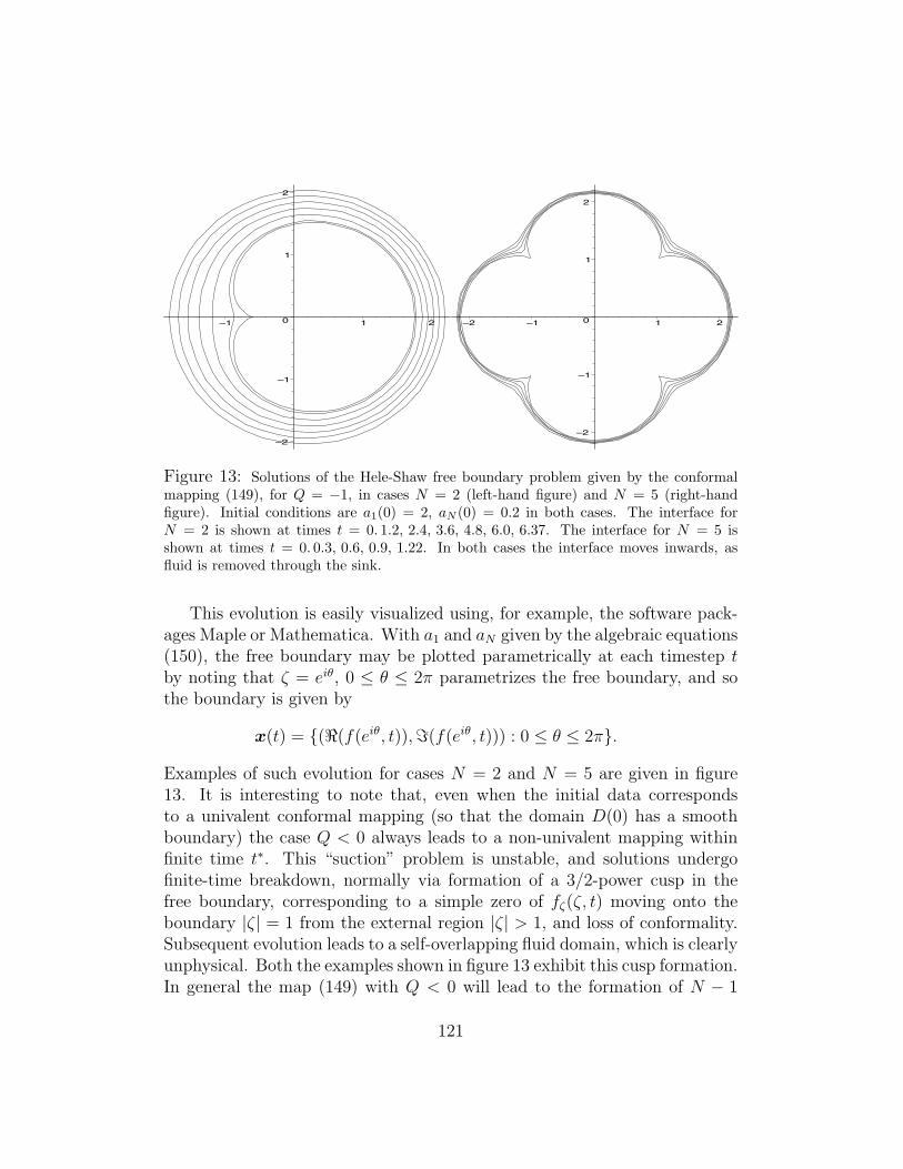
–2
–1
0
1
2
–1 1 2
–2
–1
0
1
2
–2 –1 1 2
Figure 13: Solutions of the Hele-Shaw free boundary problem given by the conformalmapping (149), for Q = −1, in cases N = 2 (left-hand figure) and N = 5 (right-handfigure). Initial conditions are a1(0) = 2, aN (0) = 0.2 in both cases. The interface forN = 2 is shown at times t = 0. 1.2, 2.4, 3.6, 4.8, 6.0, 6.37. The interface for N = 5 isshown at times t = 0. 0.3, 0.6, 0.9, 1.22. In both cases the interface moves inwards, asfluid is removed through the sink.
This evolution is easily visualized using, for example, the software pack-ages Maple or Mathematica. With a1 and aN given by the algebraic equations(150), the free boundary may be plotted parametrically at each timestep tby noting that ζ = eiθ, 0 ≤ θ ≤ 2π parametrizes the free boundary, and sothe boundary is given by
x(t) = {(<(f(eiθ, t)),=(f(eiθ, t))) : 0 ≤ θ ≤ 2π}.
Examples of such evolution for cases N = 2 and N = 5 are given in figure13. It is interesting to note that, even when the initial data correspondsto a univalent conformal mapping (so that the domain D(0) has a smoothboundary) the case Q < 0 always leads to a non-univalent mapping withinfinite time t∗. This “suction” problem is unstable, and solutions undergofinite-time breakdown, normally via formation of a 3/2-power cusp in thefree boundary, corresponding to a simple zero of fζ(ζ, t) moving onto theboundary |ζ| = 1 from the external region |ζ| > 1, and loss of conformality.Subsequent evolution leads to a self-overlapping fluid domain, which is clearlyunphysical. Both the examples shown in figure 13 exhibit this cusp formation.In general the map (149) with Q < 0 will lead to the formation of N − 1
121
cusps simultaneously in the free boundary at some finite time t∗ before allfluid has been removed from the domain.
Homework: 1. Show that a simple zero of fζ(ζ, t) on |ζ| = 1 (at ζ = 1,say) gives rise to a cusp singularity on the image curve ∂D(t). Assume, forsimplicity, that f and all derivatives evaluated at the point ζ = 1 are real.Hint: Note that, near ζ = 1 and on the boundary, ζ = eiθ, with |θ| � 1.Taylor expand this, and Taylor expand again in the conformal mapping, usingthe smallness of |θ| each time.2. Investigate the shapes described by the quadratic mapping function z =f(ζ) = aζ + bζ2 from the unit disc |ζ| ≤ 1. Assuming a, b ∈ R, can youdetermine for which values of these parameters the map is univalent on theunit disc, and for which values it is conformal?
4.2.4 The Schwarz function approach
Another approach to solving the free boundary problem, which is in manyways more elegant and powerful than that outlined above, is to use theconcept of the Schwarz function of the free boundary. Given an analyticcurve ∂D, its Schwarz function is defined to be that function g(z) such thatthe equation
z = g(z) (151)
defines the curve ∂D. For a given curve ∂D, g is analytic, at least in someneighborhood of the curve, and unique (though it is often impossible to writedown explicitly). If one has the equation of the curve in the form F (x, y) = 0then in principle the Schwarz function may be obtained by substituting forx = (z + z)/2 and y = (z − z)/(2i), and solving for z.
Example 4.13 Find the Schwarz functions of (i) the straight line y = mx+c, and (ii) the circle (x− a)2 + (y − b)2 = r2.
(i) Substituting for x and y gives
z − z2i
=m(z + z)
2+ c ⇒ z = z
(1− im1 + im
)− 2ic
1 + im≡ g(z).
(ii) Rewrite the equation of the circle in complex form as
|z − (a+ ib)|2 = r2,
122
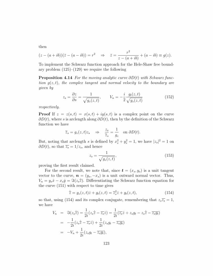
then
(z − (a+ ib))(z − (a− ib)) = r2 ⇒ z =r2
z − (a+ ib)+ (a− ib) ≡ g(z).
To implement the Schwarz function approach for the Hele-Shaw free bound-ary problem (125)–(129) we require the following
Proposition 4.14 For the moving analytic curve ∂D(t) with Schwarz func-tion g(z, t), the complex tangent and normal velocity to the boundary aregiven by
zs =∂z
∂s=
1√gz(z, t)
, Vn = − i2
gt(z, t)√gz(z, t)
(152)
respectively.
Proof If z = z(s, t) = x(s, t) + iy(s, t) is a complex point on the curve∂D(t), where s is arclength along ∂D(t), then by the definition of the Schwarzfunction we have
zs = gz(z, t)zs ⇒ zszs
=1
gzon ∂D(t).
But, noting that arclength s is defined by x2s + y2
s = 1, we have |zs|2 = 1 on∂D(t), so that zs = 1/zs, and hence
zs =1√
gz(z, t), (153)
proving the first result claimed.For the second result, we note that, since t = (xs, ys) is a unit tangent
vector to the curve, n = (ys,−xs) is a unit outward normal vector. Thus,Vn = ysx− xsy = =(zsz). Differentiating the Schwarz function equation forthe curve (151) with respect to time gives
z = gz(z, t)z + gt(z, t) = z2s z + gt(z, t), (154)
so that, using (154) and its complex conjugate, remembering that zszs = 1,we have
Vn = =(zsz) =1
2i(zsz − zsz) =
1
2i(zsz + zsgt − zsz − zsgt)
= − 1
2i(zsz − zsz) +
1
2i(zsgt − zsgt)
= −Vn +1
2i(zsgt − zsgt),
123
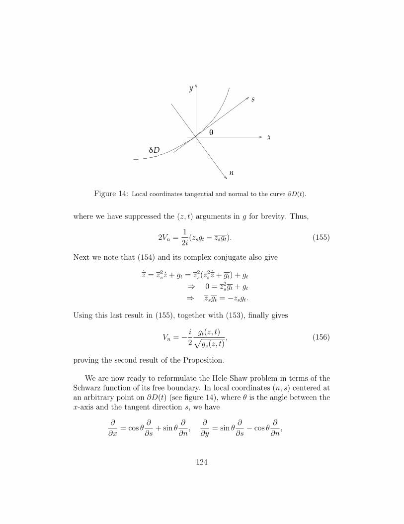
! x
sy
D"
n
Figure 14: Local coordinates tangential and normal to the curve ∂D(t).
where we have suppressed the (z, t) arguments in g for brevity. Thus,
2Vn =1
2i(zsgt − zsgt). (155)
Next we note that (154) and its complex conjugate also give
z = z2s z + gt = z2
s(z2s z + gt) + gt
⇒ 0 = z2sgt + gt
⇒ zsgt = −zsgt.
Using this last result in (155), together with (153), finally gives
Vn = − i2
gt(z, t)√gz(z, t)
, (156)
proving the second result of the Proposition.
We are now ready to reformulate the Hele-Shaw problem in terms of theSchwarz function of its free boundary. In local coordinates (n, s) centered atan arbitrary point on ∂D(t) (see figure 14), where θ is the angle between thex-axis and the tangent direction s, we have
∂
∂x= cos θ
∂
∂s+ sin θ
∂
∂n,
∂
∂y= sin θ
∂
∂s− cos θ
∂
∂n,
124
so that the derivative of the complex potential w(z, t) (see (130)) may beexpressed as follows:
∂w
∂z= px − ipy = e−iθps + ie−iθpn = zs(ps + ipn)
= −iVnzs
on ∂D
= −1
2
∂g
∂ton ∂D,
where we used the fact that the complex tangent zs = eiθ, together with theboundary conditions (126) and (127) and the results (152) above.
This last equality has been demonstrated to hold just on the boundary,∂D(t). However, the complex potential is analytic on the whole of the domainD(t), and we know that the Schwarz function is analytic at least in someneighborhood of the analytic curve ∂D(t). Thus, the principle of analyticcontinuation holds (§1.7), and we deduce that in fact the equality
∂w(z, t)
∂z= −1
2
∂g(z, t)
∂t(157)
holds wherever either function is defined, and in particular, it holds through-out the fluid domain D(t).
Equation (157) is key to finding exact solutions to the free boundaryproblem. The crucial observation is that we know w(z, t) to be analytic onD(t), except at the specified driving singularity (128). However, the Schwarzfunction of any boundary curve will in general have singularities within D(t).The above equation tells us that, any such singularities of g, which do notcoincide with a specified singularity of w(z, t) must not vary in time, sothat ∂g/∂t will not exhibit the singular behavior.
Before going ahead to solve the free boundary problem by this approachwe introduce one final piece of machinery.
Definition 4.15 (Complex conjugate function) Given a complex analyticfunction F (ζ), the complex conjugate function F (ζ) is defined by
F (ζ) = F (ζ). (158)
F (ζ) is complex analytic if ζ lies in the domain of analyticity of F .
Example 4.16 If F (ζ) =∑N
n=1 anζn then F (ζ) =
∑Nn=1 anζ
n.
125
Implementation of the Schwarz function approach
To implement the approach we return to the conformal mapping that weknow exists between the unit disc |ζ| ≤ 1 and the domain D(t), z = f(ζ, t).We again consider a flow driven by a single point source or sink, so that theonly singularity of w(z, t) is at z = 0, where w has the singular behavior(128). On the boundary the Schwarz function identity (151) leads to
g(f(ζ, t), t) = f(ζ, t) = f(ζ, t) = f(1/ζ, t), on |ζ| = 1,
using the definition of the complex conjugate function (158) above. Since weknow that each of the Schwarz function and f are analytic in some neighbor-hood of |ζ| = 1 we can use analytic continuation to deduce that the equality
g(f(ζ, t), t) = f(1/ζ, t)
holds everywhere that these functions are defined, and therefore that f(1/ζ, t)is the Schwarz function of the free boundary in the ζ-plane.
Given a conformal mapping then, with time-dependent coefficients, wecan write down the Schwarz function in the ζ-plane explicitly. We can thenfind the location of its singularities ζk(t) within the unit disc, which will cor-respond to the singularities zk(t) = f(ζk(t), t) of g(z, t) within D(t). Unlesszk(t) = 0 (the location of the only singularity of w), equation (157) tellsus that dzk/dt = 0, a condition that will yield a trivially-integrable ordi-nary differential equation for the coefficients of the mapping function. If thesingularity corresponds to z = 0 then another differential equation may beobtained by noting that the local behavior of dw/dz in (157) is
dw
dz= − Q
2πz+O(1) as z → 0,
and matching the singular behavior appropriately.The procedure is best illustrated by example, and we consider a case
that would be very difficult to solve explicitly using the Polubarinova-Galinequation (143). We take
z = f(ζ, t) =N∑n=1
an(t)ζ
ζ − bn(t)+ c(t)ζ, (159)
126
which maps the origin to the origin, and which will be analytic on |ζ| ≤ 1provided |bn(t)| ≥ 1. The Schwarz function in the ζ-plane is given by
f
(1
ζ
)=
N∑n=1
an(t)
1− bn(t)ζ+c(t)
ζ, (160)
which has singularities at points ζ = 0, ζn(t) = 1/bn(t), within the unit disc,corresponding to singularities of g(z, t) at z = 0, zn(t) = f(1/bn(t), t) withinD(t).
Near ζ = 1/bn(t) the Schwarz function in the ζ-plane satisfies
f
(1
ζ
)=
an(t)
1− bn(t)ζ+O(1),
and a local Taylor expansion of the mapping function gives
z − zn(t) = (ζ − 1/bn(t))fζ(1/bn(t), t) +O((ζ − 1/bn(t))2)
⇒ an(t)
1− bn(t)ζ= −
an(t)
bn(t)fζ
(1
bn(t), t)
z − zn(t)+O(1). (161)
By (160), this last expression gives the local form of the Schwarz functionin the z-plane, near the singularity at z = zn(t) = f(1/bn(t), t). Since thesesingularities lie within D(t), and the complex potential must be analytic atthese points, any singular behavior on the right-hand side of (157) due tothese poles must vanish. Clearly, near z = zn(t) equation (161) gives
∂g
∂t= − zn(t)
(z − zn(t))2
[an(t)
bn(t)fζ
(1
bn(t), t
)]− 1
z − zn(t)
d
dt
[an(t)
bn(t)fζ
(1
bn(t), t
)]+O(1),
so the requirement that this singular behavior be eliminated in (157) leadsto two equations for each singularity zn(t), namely
d
dt
[f(1/bn(t), t)
]= 0, n = 1, . . . , N, (162)
d
dt
[an(t)
bn(t)fζ
(1
bn(t), t
)]= 0, n = 1, . . . , N. (163)
127
To complete the solution we must also match the singular behavior at z = 0in (157), where we know dw/dz = −Q/(2πz) +O(1). Near ζ = 0 we have
f
(1
ζ, t
)=c(t)
ζ+O(1), and z = ζf ′(0, t) +O(ζ2),
⇒ g(z, t) =c(t)f ′(0, t)
z+O(1),
so that matching the singular behavior in (157) requires
d
dt(c(t)f ′(0, t)) =
Q
2π. (164)
Equations (162), (163) and (164) are immediately integrable, and give 2N+1algebraic equations for the 2N+1 unknowns an(t), bn(t), c(t), completing thesolution to the problem.
The evolution may again be depicted graphically using Maple or a similarpackage, as described for the polynomial mapping function example givenearlier. Again, the generic behavior is that for Q > 0 (injection of fluidthrough a point source), singularities of the mapping function in |ζ| ≥ 1(at ζ = bn(t)) move further away from the unit circle, corresponding to thedomain boundary becoming smoother and more circular; while for Q < 0(suction of fluid through a point sink within the flow domain) the bn(t)approach the unit circle |ζ| = 1, always reaching it within finite time. Whenthe first singularity reaches the unit circle the map ceases to be conformalon the unit disc; the boundary ∂D(t) develops a singularity, and the solutionbreaks down.
An example of the evolution is shown in figure 15, for the case N = 2.To simplify the analysis we assumed real coefficients, and a1 = −a2 = a,b1 = −b2 = b. It is easy to check in this case that equations (162) are thesame for n = 1, 2, as are equations (163), and so together with (164) wehave just three (real) equations for the three (real) unknowns a, b, c. Onceinitial conditions are specified, the equations can be solved numerically. Asthe figure shows, the evolution breaks down in finite time via the formationof two cusps in the free boundary, at the images of ζ = 1 and ζ = −1.
Homework: 1. Derive the three equations satisfied by the coefficientsa(t), b(t), c(t) in the specific example illustrated by figure 15. Show that thecusps at points ζ = ±1 form simultaneously (when they form). What is the
128
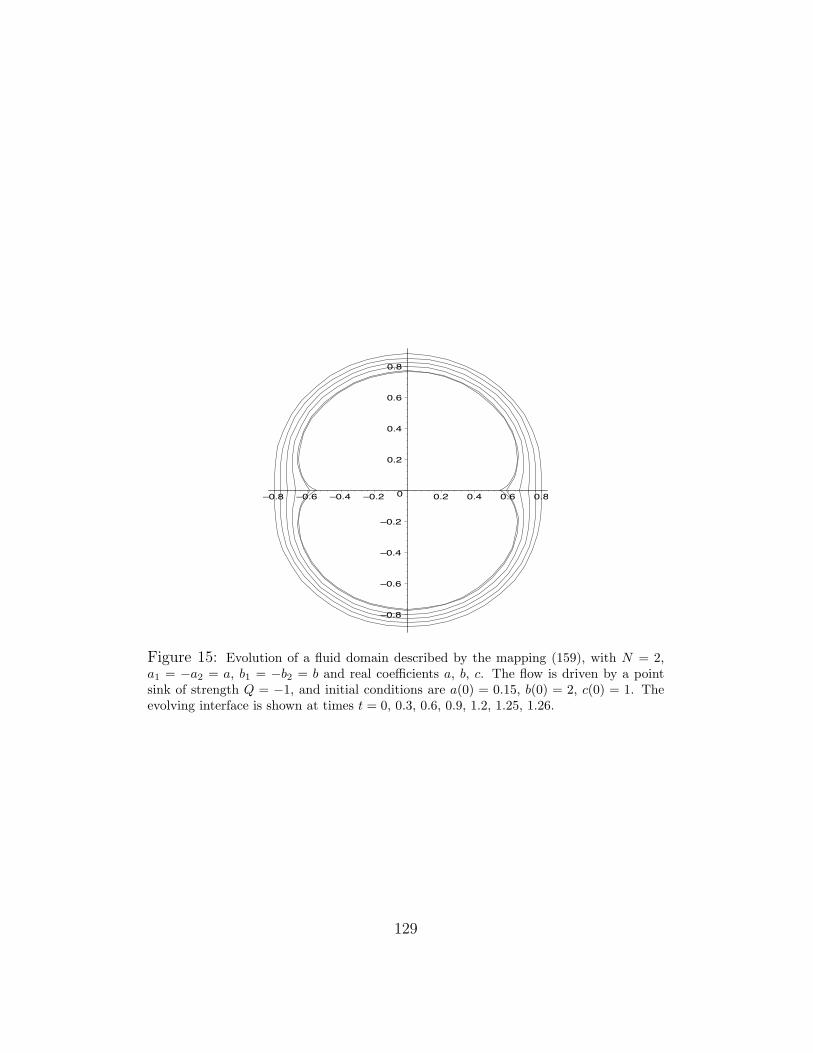
–0.8
–0.6
–0.4
–0.2
0
0.2
0.4
0.6
0.8
–0.8 –0.6 –0.4 –0.2 0.2 0.4 0.6 0.8
Figure 15: Evolution of a fluid domain described by the mapping (159), with N = 2,a1 = −a2 = a, b1 = −b2 = b and real coefficients a, b, c. The flow is driven by a pointsink of strength Q = −1, and initial conditions are a(0) = 0.15, b(0) = 2, c(0) = 1. Theevolving interface is shown at times t = 0, 0.3, 0.6, 0.9, 1.2, 1.25, 1.26.
129
large-time behavior of the governing equations when Q > 0? What are theimplications for the large-time behavior of the fluid domain?2. Implement the Schwarz function approach for the simple mapping func-tion z = f(ζ, t) = a(t)ζ.3. (Harder) Try extending this to the flow described by the quadratic map-ping function z = f(ζ, t) = a(t)ζ + b(t)ζ2.
4.3 Other applications
We conclude by mentioning some other real-world problems in which complexanalysis approaches can be very useful.
4.3.1 2D Stokes flow (and elasticity)
Stokes flow, or slow viscous flow, describes the situation of a Newtonian fluidin which the Reynolds number7 is very small, Re � 1. This means thatthe inertial terms in the Navier-Stokes equations may be neglected, and theflow is dominated by viscous effects. The governing equations for the fluidvelocity u and pressure p are, in suitably scaled variables,
∇p = ∇2u, ∇ · u = 0
and writing the velocity field in terms of a streamfunction ψ, u = (ψy,−ψx)(so that the incompressibility condition ∇ ·u = 0 is automatically satisfied),we find
∇p = (ψxxy + ψyyy,−ψxxx − ψxyy).
Since the curl of a gradient field is always zero, ∇ ∧ (∇p) = 0, we obtainfinally
∇2(∇2ψ) = 0, or ∇4ψ = 0.
This equation is known as the bilaplacian or biharmonic equation and, sim-ilarly to Laplace’s equation, its solutions are expressible in complex variableform. To see this note that the Laplace operator may be written as
∂2
∂x2+
∂2
∂y2= 4
∂2
∂z∂z,
7The Reynolds number of a flow is a dimensionless number characterizing the flow,defined by Re = ρUL/µ. where ρ is the fluid density, U is a typical flow velocity, L is atypical lengthscale associated with the flow, and µ is the fluid’s viscosity.
130
so that if ∇2ψ = q,
∇2q = 0 ⇒ ∂2q
∂z∂z= 0 ⇒ q = 4(f(z) + g(z)).
Then
∂2ψ
∂z∂z= f(z) + g(z)
⇒ ∂ψ
∂z= zf(z) +
∫ z
g(z) dz + h(z) = zf(z) +G(z) + h(z)
⇒ ψ = z
∫ z
f(z) dz + zG(z) +
∫ z
h(z) dz + j(z)
= zF (z) + zG(z) +H(z) + J(z).
We note that, since ψ is a real function we must have ψ = ψ, which requiresF (z) = G(z) = G(z) and H(z) = J(z) = J(z), so that finally
ψ = 2<(zF (z) +H(z)).
This is known as the Goursat representation of biharmonic functions.Once determined, the functions F and H, which are complex analytic on theflow domain away from any specified driving singularities of the flow, fullyspecify the fluid flow. In general, determination of F and H requires thatwe specify appropriate boundary conditions. For free boundary problems,like those discussed in §4.2 above, it turns out that (as was the case for theHele-Shaw problem) the boundary conditions for a simply-connected flowdomain have a convenient form when expressed in terms of the complex vari-able representation, and exact time-dependent solutions to moving boundaryproblems may be obtained.
The full details of this procedure are beyond the scope of this course.Here we just give a few examples of flows in unbounded domains, obtainedby choosing suitable forms for F and H.
Example 4.17 (Rigid-body rotation) Find the Goursat functions F and Hfor a flow in rigid-body rotation about the origin.
Rigid-body rotation with constant angular velocity ω = ωk corresponds toa velocity field
u = ω(−y, x)
131
so that the streamfunction ψ = −ω(x2 + y2) = −ωzz, up to an arbitraryadditive constant. Thus, F (z) = −ωz/2 and H(z) = 0.
Example 4.18 (Rigid-body translation) Find the Goursat functions F andH for a flow in rigid-body translation, u = (u0, v0).
Here ψ = u0y − v0x = <(−iu0z − v0z), so that F (z) = 0 and H(z) =−i(u0 − iv0)z/2.
A linear combination of rigid body rotation and translation may be ob-tained by adding the two streamfunctions obtained above, taking F (z) =−ωz/2 and H(z) = −i(u0 − iv0)z/2.
Homework: Find the Goursat functions associated with:1. The streamfunction for a vortex, ψ = (Γ/2π) log r.2. The streamfunction for a collection of vortices of strengths Γj at points(xj, yj) in the flow.
4.4 Hodograph Transformation and the potential plane
A frequently-used technique in fluid-dynamical problems for which a complexpotential exists is to work in the complex plane of the complex potential, orits derivative with respect to z. One can then attempt to find the mappingz(w) between the planes, and hence invert to obtain w(z).
The procedure is best illustrated by example, and we use a classical prob-lem from the Hele-Shaw free boundary literature, due to Saffman and Taylor[9]. These authors carried out an experiment in which air was forced into along, rectangular Hele-Shaw cell, initially filled with viscous fluid (glycerine).The air is observed to form a steadily-propagating ”finger”, traveling downthe rectangle, as shown in figure 16 (taken from the original paper; sub-figure8).
The authors modeled the experiment using the theory of the classicalHele-Shaw free boundary problem presented in §4.2. The idealized geom-etry is shown in figure 17. The cell is taken to be infinitely long in thex-direction, with confining walls at y = ±1. We consider a semi-infinite,steadily-translating finger of air, moving with speed U and with its nose atthe origin, and flat sides y → ±λ as x→ −∞.
In §4.2 we worked with the complex potential whose real part was the fluidpressure, p = <(w), where u = −∇p; here, to conform to standard usage,
132
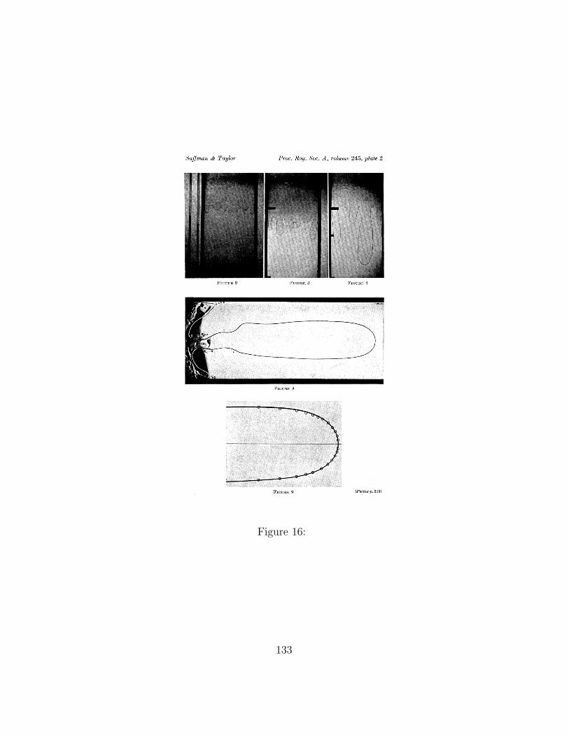
Figure 16:
133
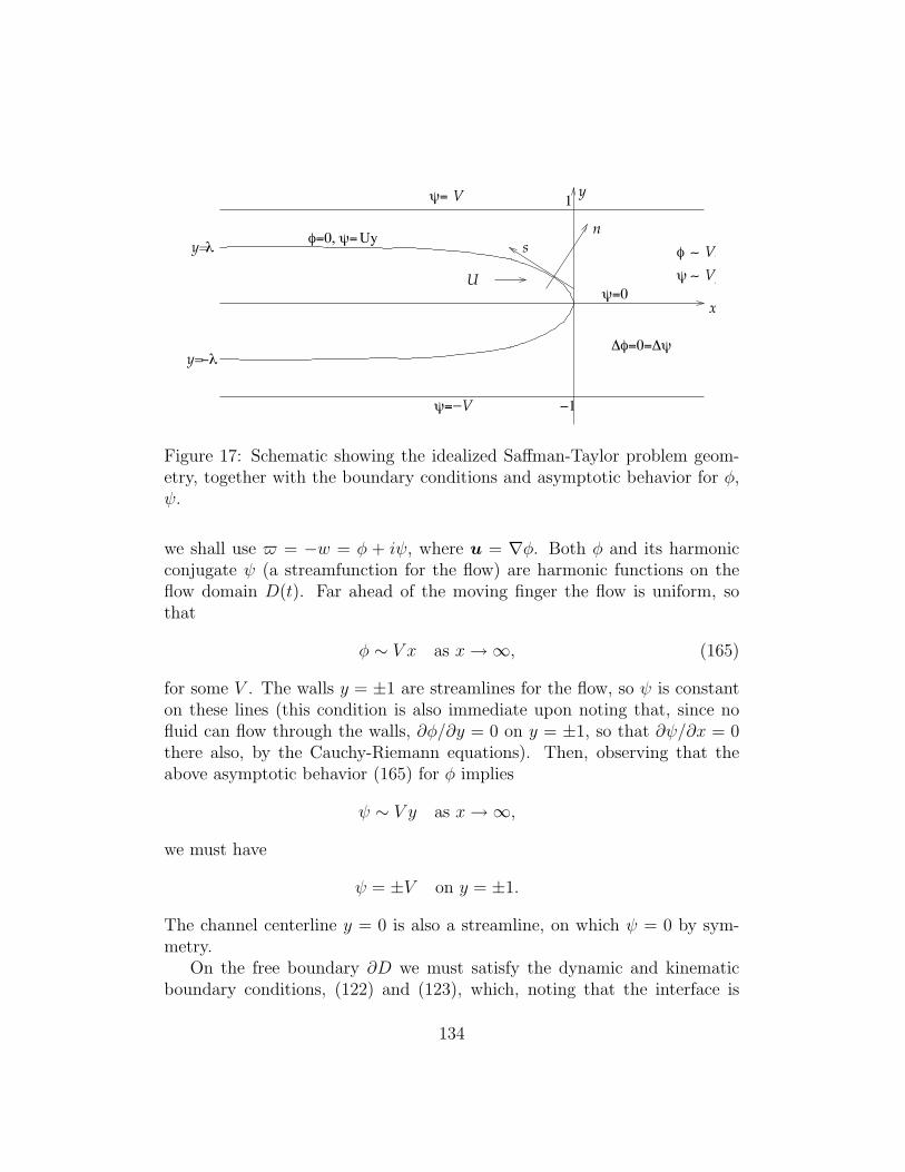
y=!"
y="
#=
#=
1 y
!1
#=0
$ %
# %
x
VyVx
ns$=0, #=
&$=0=&#
V
−V
Uy
U
Figure 17: Schematic showing the idealized Saffman-Taylor problem geom-etry, together with the boundary conditions and asymptotic behavior for φ,ψ.
we shall use $ = −w = φ + iψ, where u = ∇φ. Both φ and its harmonicconjugate ψ (a streamfunction for the flow) are harmonic functions on theflow domain D(t). Far ahead of the moving finger the flow is uniform, sothat
φ ∼ V x as x→∞, (165)
for some V . The walls y = ±1 are streamlines for the flow, so ψ is constanton these lines (this condition is also immediate upon noting that, since nofluid can flow through the walls, ∂φ/∂y = 0 on y = ±1, so that ∂ψ/∂x = 0there also, by the Cauchy-Riemann equations). Then, observing that theabove asymptotic behavior (165) for φ implies
ψ ∼ V y as x→∞,
we must have
ψ = ±V on y = ±1.
The channel centerline y = 0 is also a streamline, on which ψ = 0 by sym-metry.
On the free boundary ∂D we must satisfy the dynamic and kinematicboundary conditions, (122) and (123), which, noting that the interface is
134
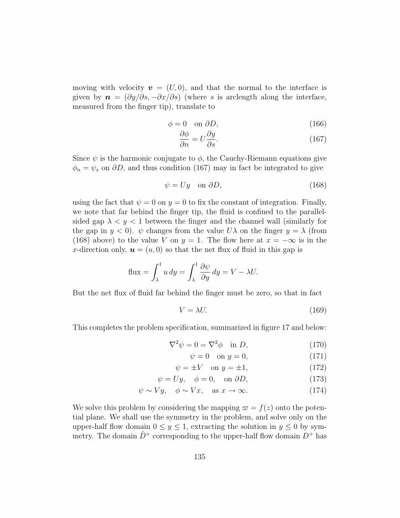
moving with velocity v = (U, 0), and that the normal to the interface isgiven by n = (∂y/∂s,−∂x/∂s) (where s is arclength along the interface,measured from the finger tip), translate to
φ = 0 on ∂D, (166)
∂φ
∂n= U
∂y
∂s. (167)
Since ψ is the harmonic conjugate to φ, the Cauchy-Riemann equations giveφn = ψs on ∂D, and thus condition (167) may in fact be integrated to give
ψ = Uy on ∂D, (168)
using the fact that ψ = 0 on y = 0 to fix the constant of integration. Finally,we note that far behind the finger tip, the fluid is confined to the parallel-sided gap λ < y < 1 between the finger and the channel wall (similarly forthe gap in y < 0). ψ changes from the value Uλ on the finger y = λ (from(168) above) to the value V on y = 1. The flow here at x = −∞ is in thex-direction only, u = (u, 0) so that the net flux of fluid in this gap is
flux =
∫ 1
λ
u dy =
∫ 1
λ
∂ψ
∂ydy = V − λU.
But the net flux of fluid far behind the finger must be zero, so that in fact
V = λU. (169)
This completes the problem specification, summarized in figure 17 and below:
∇2ψ = 0 = ∇2φ in D, (170)
ψ = 0 on y = 0, (171)
ψ = ±V on y = ±1, (172)
ψ = Uy, φ = 0, on ∂D, (173)
ψ ∼ V y, φ ∼ V x, as x→∞. (174)
We solve this problem by considering the mapping $ = f(z) onto the poten-tial plane. We shall use the symmetry in the problem, and solve only on theupper-half flow domain 0 ≤ y ≤ 1, extracting the solution in y ≤ 0 by sym-metry. The domain D+ corresponding to the upper-half flow domain D+ has
135
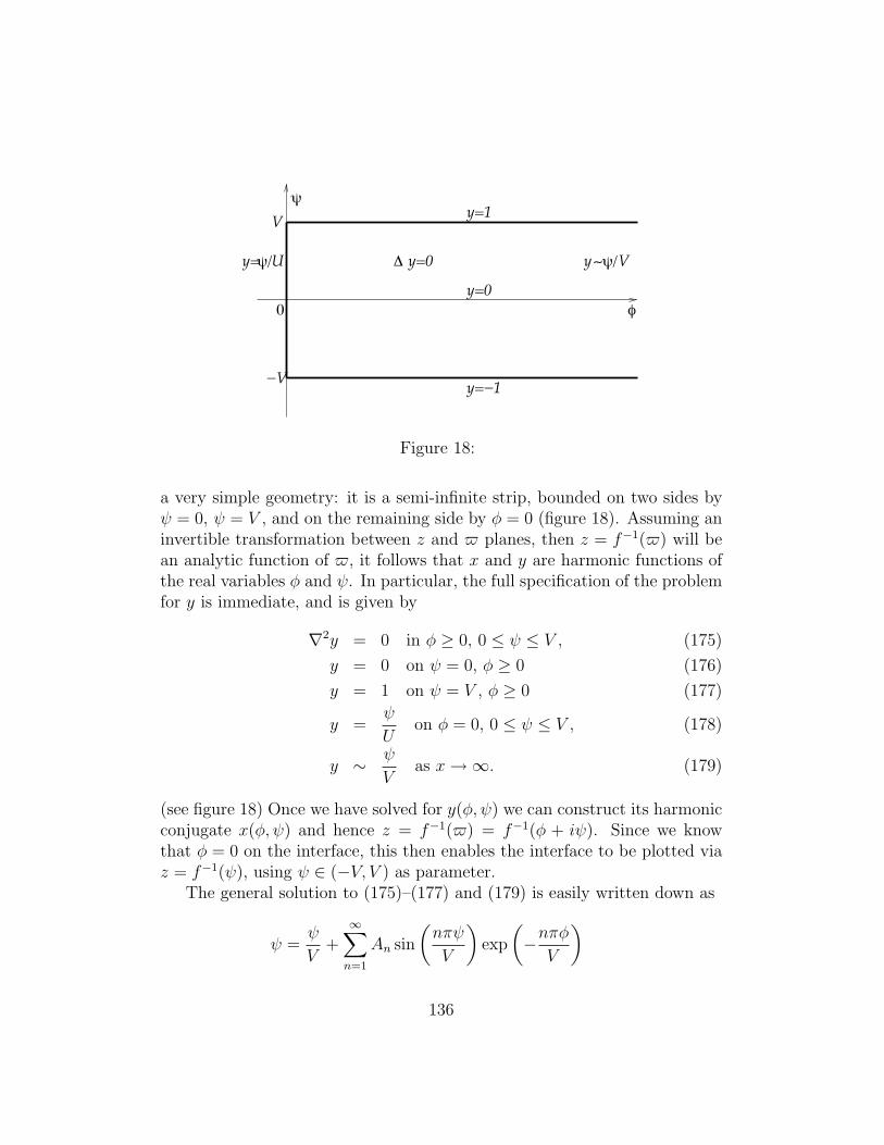
!
"
0
y=0
y=0
y=1
y=−1
y="/ # y$"/U
V
−V
V
Figure 18:
a very simple geometry: it is a semi-infinite strip, bounded on two sides byψ = 0, ψ = V , and on the remaining side by φ = 0 (figure 18). Assuming aninvertible transformation between z and $ planes, then z = f−1($) will bean analytic function of $, it follows that x and y are harmonic functions ofthe real variables φ and ψ. In particular, the full specification of the problemfor y is immediate, and is given by
∇2y = 0 in φ ≥ 0, 0 ≤ ψ ≤ V , (175)
y = 0 on ψ = 0, φ ≥ 0 (176)
y = 1 on ψ = V , φ ≥ 0 (177)
y =ψ
Uon φ = 0, 0 ≤ ψ ≤ V , (178)
y ∼ ψ
Vas x→∞. (179)
(see figure 18) Once we have solved for y(φ, ψ) we can construct its harmonicconjugate x(φ, ψ) and hence z = f−1($) = f−1(φ + iψ). Since we knowthat φ = 0 on the interface, this then enables the interface to be plotted viaz = f−1(ψ), using ψ ∈ (−V, V ) as parameter.
The general solution to (175)–(177) and (179) is easily written down as
ψ =ψ
V+∞∑n=1
An sin
(nπψ
V
)exp
(−nπφ
V
)
136
where the An are determined from the remaining boundary condition (178),which requires
ψ
(1
U− 1
V
)=∞∑n=1
An sin
(nπψ
V
).
The coefficients are extracted by the usual Fourier series method of multi-plying both sides of this equation by sin(mπψ/V ) and integrating betweenψ = 0 and ψ = V , which leads to
Am =2(−1)m
mπ(1− λ),
recalling that V = λU . Thus,
y =ψ
V+
2(1− λ)
π
∞∑m=1
(−1)m
msin
(mπψ
V
)exp
(−mπφ
V
),
which, noting that
sin
(mπψ
V
)exp
(−mπφ
V
)= −=
[exp
(−mπV
(φ+ iψ))]
we recognise as
y = =
[$
V+
2(1− λ)
π
∞∑m=1
(−1)m+1
mexp
(−mπ$
V
)]
= =[$
V+
2(1− λ)
πln(
1 + exp(−π$V
))].
We still have a real constant to choose when extracting z = x + iy, butrecalling that we want z = 0 when $ = 0 fixes this, and we finally obtain
z = f−1($) =$
V+
2(1− λ)
πln
[1
2
(1 + exp
(−π$V
))]. (180)
The complex potential $ is thus implicitly determined as a function of zand, as stated earlier, we can plot the interface by setting φ = 0 in (180),and plotting the parametric curve
(x, y) = {(<(f−1($)),=(f−1($))) : $ = iψ, ψ ∈ (−V, V )}.
137
A The Schwarz-Christoffel transformation
As mentioned earlier, the Riemann mapping theorem, though it guaranteesthe existence of a conformal mapping between any two simply-connecteddomains in the complex plane, gives us no clue as to how to construct suchmappings. There is, however, one notable and quite general case in which theconformal mapping can be constructed explicitly: when we are mapping froma nice canonical domain (the upper half-plane, in the usual theorem state-ment) onto the interior of an arbitrary polygon. The Schwarz-Christoffeltransformation gives a recipe for doing exactly this. Before stating and(non-rigorously) proving the theorem, we outline some of the important ideasbehind the construction of the transformation.
The theorem makes use of a variant of the Schwarz reflection principle,which enables us to analytically continue functions across boundaries or linesin the complex plane.
A.1 Schwarz reflection principle
Although this principle is really quite general, we shall consider it only in acouple of special cases. First, consider a function f(ζ), analytic on the upperhalf-plane D+. Then, the function f , defined for any point ζ in the lowerhalf-plane D− by
f(ζ) = f(ζ), (181)
is in fact analytic on D−. That f is defined on D− is confirmed by checkingthat ζ ∈ D− ⇐⇒ ζ ∈ D+; and analyticity can be demonstrated by appealingto the Cauchy-Riemann equations. Writing f(ζ) = u(ξ, η) + iv(ξ, η) andf(ζ) = u(ξ, η) + iv(ξ, η), the definition (181) gives
u(ξ, η) = u(ξ,−η), v(ξ, η) = −v(ξ,−η),
and hence for ξ + iη ∈ D−, ξ − iη ∈ D+, we have
uξ(ξ, η) = uξ(ξ,−η) = vη(ξ,−η) = vη(ξ, η),
uη(ξ, η) = −uη(ξ,−η) = vξ(ξ,−η) = −vξ(ξ, η),
confirming that f is analytic on the domain D− as claimed. (We note forlater reference that the function f defined here is often written as f , and isknown as the complex conjugate function to f .)
138
A similar procedure may be carried out for the unit disc, B(0; 1). If f(ζ)is analytic on |ζ| ≤ 1 then we can define a function f , analytic outside theunit disc
f(ζ) = f(1/ζ) |ζ| ≥ 1.
In each of these examples, the new functions f rely on “reflecting” the pointsin the boundary curve – in the first case, ζ is the reflection of ζ in the realaxis =(ζ) = 0, while in the second case, 1/ζ is the reflection of ζ in the unitcircle |ζ| = 1. These are sensible definitions of reflections because, in eithercase, equality of the point with its reflection defines the boundary curve.
Returning to the first case, suppose we also know that the function ftakes real values on the real axis, that is, f(ξ) ∈ R for ξ ∈ R. Then in thiscase we have equality of f and f on the boundary,
f(ξ) = f(ξ) = f(ξ) = f(ξ) for ξ ∈ R,
and since both f and f are analytic in some neighborhood of the boundaryand coincide there, it follows that f represents the analytic continuation off into D−.
We may generalize this notion somewhat. Suppose we only know thatf is real along some line segment l of the real axis. Then the process ofdefining the function f will again lead to an analytic continuation of f , butthe extended function (which takes values f(ζ) for ζ in D+ and f(ζ) for ζ inD−) will be analytic on the real axis only along segment l, and not elsewhereon this axis. An obvious example of such a function is given by f(ζ) =
√ζ,
defined for points ζ ∈ D+ by
f(ζ) = f(reiθ) = r1/2eiθ/2, 0 ≤ θ ≤ π.
This is real along l = [0,∞) but not along (−∞, 0), and taking values atpoints ζ = reiθ ∈ D− (−π < θ < 0) given by
f(reiθ) = f(re−iθ) = r1/2e−iθ/2 = r1/2eiθ/2,
we see that the composite function defined by f and f is analytic on theζ-plane, except along the real negative axis (which of course represents abranch-cut in the plane), where it is discontinuous.
In the above, we used the fact that the function f was real along thereal axis, or segments of it, in order to define the analytic continuation.
139
Considering z = f(ζ) as a conformal mapping, this means that (part of)the real axis in the ζ-plane maps to (part of) the real axis in the z-plane.However, since it is trivial to translate and rotate a line segment, we can seethat we could easily carry out the same procedure of analytic continuationfor the case in which z = f(ζ) maps the real ζ-axis, or part of it, to anystraight line in the z-plane. The general equation of such a straight line is
<(βz) = γ, β ∈ C (β 6= 0), γ ∈ R,
and we suppose this is the image of ζ = ξ ∈ R under f , so that we have
βf(ξ) + βf(ξ) = 2γ, ξ ∈ R. (182)
Consider now the function f defined for ζ ∈ D− by
f(ζ) =2γ
β− β
βf(ζ).
For ζ ∈ D−, ζ ∈ D+, and as before, f may be seen to define a functionanalytic on D−. Moreover, letting ζ approach the boundary between D+
and D−, ζ = ξ ∈ R, we have
f(ξ) =2γ
β− β
βf(ξ) =
2γ
β− 1
β(2γ − βf(ξ)) = f(ξ).
Thus here, as before, f represents an analytic continuation of the function fonto the lower half-plane D−; and image points z = f(ζ), ζ ∈ D−, lie in areflected region to the other side of the line <(βz) = γ in the z-plane.
Before going on to state and prove the Schwarz-Christoffel theorem, wenote that the above discussion extends to analytic continuation across linesegments, as well as infinite lines. As with the simple example above, whenthe continuation is across line segments, the resulting composite function ingeneral has branch-points.
A.2 The Schwarz-Christoffel theorem
Theorem A.1 (Schwarz-Christoffel) Let Γ be the piecewise linear boundaryof a polygon in the z-plane, with vertices Aj (j = 1, . . . , n) and associatedinterior angles παj. Then, the transformation z = f(ζ) defined by
df
dζ= CΠn
j=1(ζ − aj)αj−1, (183)
140
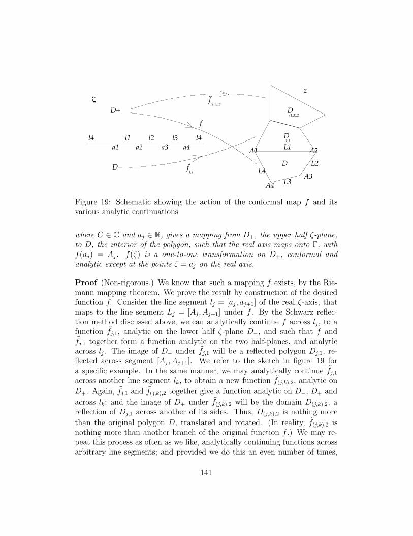
D
D
a2 a4a3a1
D+
D−A3
l1L1
L2
L3
l4 l2 l3 l4
!z
(1,3),2
A4
L4
1,1D
A2A1~f1,1
~f(1,3),2
f
Figure 19: Schematic showing the action of the conformal map f and itsvarious analytic continuations
where C ∈ C and aj ∈ R, gives a mapping from D+, the upper half ζ-plane,to D, the interior of the polygon, such that the real axis maps onto Γ, withf(aj) = Aj. f(ζ) is a one-to-one transformation on D+, conformal andanalytic except at the points ζ = aj on the real axis.
Proof (Non-rigorous.) We know that such a mapping f exists, by the Rie-mann mapping theorem. We prove the result by construction of the desiredfunction f . Consider the line segment lj = [aj, aj+1] of the real ζ-axis, thatmaps to the line segment Lj = [Aj, Aj+1] under f . By the Schwarz reflec-tion method discussed above, we can analytically continue f across lj, to afunction fj,1, analytic on the lower half ζ-plane D−, and such that f andfj,1 together form a function analytic on the two half-planes, and analyticacross lj. The image of D− under fj,1 will be a reflected polygon Dj,1, re-flected across segment [Aj, Aj+1]. We refer to the sketch in figure 19 fora specific example. In the same manner, we may analytically continue fj,1across another line segment lk, to obtain a new function f(j,k),2, analytic on
D+. Again, fj,1 and f(j,k),2 together give a function analytic on D−, D+ and
across lk; and the image of D+ under f(j,k),2 will be the domain D(j,k),2, areflection of Dj,1 across another of its sides. Thus, D(j,k),2 is nothing more
than the original polygon D, translated and rotated. (In reality, f(j,k),2 isnothing more than another branch of the original function f .) We may re-peat this process as often as we like, analytically continuing functions acrossarbitrary line segments; and provided we do this an even number of times,
141
the resulting function fj ,2m(ζ) (where j is a vector of length 2m representing
the sequence of Schwarzian reflections used) takes the upper half ζ-plane D+
onto a rotation and translation of D. Therefore, fj ,2m(ζ) is linearly related
to f ,
fj ,2m(ζ) = Bj ,2mf(ζ) + Cj ,2m, Bj ,2m = exp(iβj ,2m),
and it follows that the function
g(ζ) =f ′′j ,2m(ζ)
f ′j ,2m
(ζ)≡ f ′′(ζ)
f ′(ζ)
is in fact single-valued, regardless of whether we use f or any one of the fj ,2mto define it.
We now note that g(ζ) is in fact real-valued on the real ζ-axis. Thisfollows because the piecewise linear nature of the boundary mapping meansthat f(ξ) = F (ξ)eiγj , for F (ξ) a real function, and γj a real constant on eachline segment lj. Therefore, on the real axis f ′(ζ) = f ′(ξ) = F ′(ξ)eiγj andf ′′(ζ) = f ′′(ξ) = F ′′(ξ)eiγj , so that
g′′(ζ) =f ′′(ξ)
f ′(ξ)=F ′′(ξ)
F ′(ξ)∈ R.
This fact, together with the uniqueness of g, tells us that, although thereare many possible branches for f when analytically continued across linesegments, there is one unique analytic function g(ζ) = f ′′(ζ)/f ′(ζ); and thisfunction may be analytically continued across the entire real axis, since ittakes real values there, by the usual prescription
g(ζ) = g(ζ),
to give a function analytic on the entire ζ-plane except at the points ζ = aj.Near aj we know that the map f must describe the polygonal vertex Aj,
and so locally f has the form
f(ζ) = Aj + (ζ − aj)αj(c(0)j + c
(1)j (ζ − aj) + · · ·),
where c(0)j ∈ C 6= 0 (we know that f maps aj to Aj, and that at this point
angles are multiplied by the factor αj, since the straight line, with “angle”
142
π, must map to a corner of angle παj). It follows that g(ζ) = f ′′(ζ)/f ′(ζ)has a simple pole at the point aj, of residue (αj − 1),
g(ζ) =αj − 1
ζ − aj(1 +O(ζ − aj)) . (184)
Apart from these poles, g has no other singularities, and
G(ζ) := g(ζ)−n∑j=1
αj − 1
(ζ − aj)
defines an entire function. Since we assume for the moment that no vertexof the polygon is at infinity, then f(ζ) is analytic at infinity and so G isin fact a bounded entire function, and so is equal to some constant c, byLiouville’s theorem. But since f itself is bounded and analytic at infinity,it has a regular Taylor series in powers of 1/ζ there; and it follows thatg(ζ) = f ′′(ζ)/f ′(ζ) → 0 as |ζ| → ∞, and hence also that G(ζ) → 0 as|ζ| → ∞. Thus G(ζ) ≡ 0, and
f ′′(ζ)
f ′(ζ)=
n∑j=1
αj − 1
(ζ − aj).
Integration of this result leads to (183).
A.2.1 Notes on the theorem
1. Since the sum of the exterior angles of a polygon is 2π, and the exteriorangle at the jth vertex is π − παj, it follows that
n∑j=1
αj = n− 2. (185)
2. The correspondence of three, and only three, boundary points, canbe prescribed arbitrarily (see theorem 3.20). So, for example, givena polygon with vertices Aj, we can fix a1, a2 and a3 at will, but theremaining aj (sometimes called accessory parameters) cannot be chosenand must be determined somehow (this can be difficult).
143
3. Although the proof as given does not carry through to the case in whichone of the vertices Aj lies at infinity (consider the step where we arguefor the local form of f near one of the aj), the result of the theoremis good for this case also. The case αj = 0 corresponds to a (parallel-sided) strip, while an open sector-type domain corresponds to αj < 0.We just need to argue that, local to aj, g(ζ) = f ′′(ζ)/f ′(ζ) has theappropriate form as given by (184). This is straightforward enough todo for the “open sector” case, where the local form of f may again bewritten down, but requires a little more thought for the strip-like case.
4. The next possible flaw in the theorem’s proof is: What if one of thepreimage points ak lies at infinity? We saw in point 2 above that wecannot always specify the aj at will, so we cannot be sure that theyare always at finite points. To address this point, we consider thetransformation
ζ = ak −1
w,
which takes ζ = ak to w =∞, while the other aj are mapped to finitepoints bj = 1/(ak − aj) on the real w-axis. We can now investigate theform of the mapping z = F (w) = f(ζ(w)) from the upper half w-planeto the polygon. We have
f ′(ζ)ζ ′(w) = F ′(w), and ζ ′(w) =1
w2.
Also, for j 6= k,
ζ − aj =ak − ajw
(w − bj), while ζ − ak = − 1
w.
Substituting these results in (183) gives
w2F ′(w) = C
(1
w
)αk−1
Πj 6=k
(1
w
)αj−1
(w − bj)αj−1
⇒ F ′(w) = CΠj 6=k(w − bj)αj−1,
using remark (1) above. Near infinity we see that
F ′(w) = Cw−(αk+1)(
1 +p1
w+p2
w2+ · · ·
),
so for αk > 0 w =∞ maps to a finite point, as usual.
144
A.2.2 Examples
Example A.2 Find a mapping from the upper half ζ-plane to the semi-infinite strip −k < <(z) < k, =(z) > 0.
Here we have freedom to choose the correspondence between points, andwriting A1 = −k, A2 = k and A3 = ∞, we take a1 = −1, a2 = 1, a3 = ∞.With interior angles π/2 at A1 and A2 we have α1 = α2 = 1/2, and formula(183) then gives
f ′(ζ) = C(ζ + 1)−1/2(ζ − 1)−1/2 =C√
1− ζ2
which, on integrating, gives
f(ζ) = C sin−1 ζ + C1.
Knowing that f(±1) = ±k fixes C1 = 0, C = 2k/π, so that
z = f(ζ) =2k
πsin−1 ζ, or ζ = sin
πz
2k.
145
B Fluid dynamics
The state of a flowing liquid (or gas) may be characterized by specifying thevelocity of each fluid element x(t), as a function of time:
dx
dt= u(x, t)
(think of a fluid element as an infinitesimal dyed blob of fluid). The equationsgoverning a two-dimensional viscous incompressible fluid with velocity fieldu(x, t) = (u(x, y, t), v(x, y, t)) are, in the absence of external body forcessuch as gravity,
ρdu
dt≡ ρ(ut + uux + vuy) = −px + µ(uxx + uyy), (186)
ρdv
dt≡ ρ(vt + uvx + vvy) = −px + µ(vxx + vyy), (187)
∇ · u = ux + vy = 0, (188)
where the scalar function p(x, y, t) is the pressure in the fluid at any givenpoint. Equations (186) and (187) represent the momentum balance for thefluid (essentially Newton’s 2nd law, ”mass times acceleration equals force”for the fluid, in both x and y directions), while (188) represents the incom-pressibility condition. These equations, which collectively are known as theNavier-Stokes equations, can be derived by considering the rates of changeof momentum and mass for an arbitrary material fluid volume; see for exam-ple Ockendon & Ockendon [7].
We may transform the problem to dimensionless form by introducingrepresentative scalings for each of the physical quantities. Suppose that Lis a representative lengthscale for the flow, and that U is a representativevelocity scale (for example, if we are considering the flow generated by movinga sphere through a large volume of stationary fluid then the representativelengthscale would be the sphere radius, while the velocity scale would be thespeed of translation of the sphere). We anticipate that the representativetimescale for the disturbances generated will be T = L/U . If we choose anarbitrary pressure scaling Π for the moment, then introducing our scalings
(x, y) = L(x′, y′), (u, v) = U(u′, v′), t = (L/U)t′, p = Πp′
into (186) gives (on dropping the primes)
ρU2
L(ut + uux + vuy) = −Π
Lpx +
µU
L2(uxx + uyy)
146
⇒ ρUL
µ(ut + uux + vuy) = −ΠL
µUpx + (uxx + uyy). (189)
The quantity ρUL/µ appearing on the left-hand side here is a very importantparameter in fluid mechanics: the Reynolds number of the flow, which wewrite as Re. The left-hand side of this equation represents the inertia ofthe fluid. With our assumptions of no external forces acting, the flow isalways being driven by the pressure gradient, so the term px will always beimportant in the equations. The remaining 2nd derivative terms on the right-hand side are the viscous forces (essentially internal friction) within the fluid.One possibility is that each of these three effects (inertia, pressure, viscous)could be equally important – in this case there is no real simplification of theproblem, and it’s very difficult to find exact solutions. Another possibility isthat the pressure terms balance only one of the other two: inertial or viscousterms. We consider the two cases below.
B.1 Case 1: Inviscid fluid dynamics
If pressure balances inertia, with viscous effects much smaller, then thismeans that the Reynolds number must be very large, Re � 1. In thiscase the appropriate scaling for the pressure is Π = µURe/L = ρU2, and(189) becomes
(ut + uux + vuy) = −px +1
Re(uxx + uyy).
For Re� 1 this can be approximated by the “inviscid” form of the equation,
(ut + uux + vuy) = −px, (190)
with (187) similarly becoming
(vt + uvx + vvy) = −py,
and (188) remaining unchanged,
ux + vy = 0.
Suppose now that we have the situation considered in §4.1, where inaddition to being 2D and incompressible, the flow is also irrotational, ω =∇ · u = 0. Then with this condition and (188) we have
ux + vy = 0, vx − uy = 0,
147
so that u−iv is an analytic function, by the Cauchy-Riemann theorem. Sinceanalytic functions are infinitely differentiable (and integrable) we may write
dw
dz= u− iv, (191)
(as usual z = x+ iy) for some complex analytic function w(z) = φ(x, y, t) +iψ(x, y, t). Since, differentiating w with respect to z we have
dw
dz= φx + iψx = φx − iφy (192)
(on use of the Cauchy-Riemann equations). Comparing (191) and (192), wesee that
(u, v) = (φx, φy) = ∇φ
and the function φ is a velocity potential for the flow. The function w = φ+iψis the complex potential. As the real part of a complex analytic function, φis harmonic, and thus solutions of the 2D Laplace equation represent possi-ble solutions to inviscid fluid dynamics. Returning to (190) and (191), thepressure field satisfies
∂
∂x
(p+ φt +
1
2(φ2
x + φ2y)
)= 0 =
∂
∂y
(p+ φt +
1
2(φ2
x + φ2y)
).
Integration of these leads to the well-known Bernoulli condition for inviscidflow which, in the special case of steady flow (∂/∂t = 0) takes the form
p = constant− 1
2(φ2
x + φ2y) = constant− 1
2|u|2.
B.2 Case 2: Very viscous flow (Stokes flow)
Returning to (189), the other possibility we mentioned is that the drivingpressure gradient balances viscous forces, with inertial terms being muchsmaller. In this case the Reynolds number is very small, Re � 1, and wechoose the pressure scale Π to be Π = µU/L, so that (189) becomes
Re(ut + uux + vuy) = −px + (uxx + uyy),
148
with a similar expression arising from the equation (187):
Re(vt + uvx + vvy) = −py + (vxx + vyy),
Neglecting the left-hand side in these equations gives the equations of (two-dimensional) slow viscous flow, known as the Stokes equations:
px = uxx + uyy, py = vxx + vyy, ux + vy = 0.
149
References
[1] Ablowitz, M.J., Fokas, A.S. Complex variables: Introduction and Ap-plications (2nd Edition) Cambridge University Press (2003).
[2] Abramowitz, M., Stegun, I.A. Handbook of mathematical func-tions. Dover, New York (1972).
[3] Acheson, D.J. Elementary Fluid Dynamics. Oxford University Press(2006).
[4] Batchelor, G.K. An Introduction to Fluid Dynamics. CambridgeUniversity Press (2000).
[5] Gradshteyn, I.S., Ryzhik, I.M. Table of integrals, series and prod-ucts (6th Edition). Academic Press, London (2000).
[6] Hele-Shaw, H.S. The flow of water. Nature 58, 34-36 (1898).
[7] Ockendon, H., Ockendon, J.R. Viscous flow. Cambridge UniversityPress (1995).
[8] Ockendon, J.R., Howison, S.D., Lacey, A.A., Movchan, A.Applied Partial Differential Equations (Revised Edition). Oxford Uni-versity Press (2003).
[9] Saffman, P.G., Taylor, G. The penetration of a fluid into a porousmedium or Hele-Shaw cell containing a more viscous liquid. Proc. Roy.Soc. Lond. A, 245, 312-329 (1958).
[10] Spiegel, M.R., Liu, J. Mathematical handbook of formulas and tables(2nd Edition). Schaum’s Outline Series, McGraw-Hill, New York (1999).
150