mathematical behavioural finance a mini course
TRANSCRIPT

Mathematical Behavioural Finance A Mini Course
Mathematical Behavioural FinanceA Mini Course
Xunyu Zhou
January 2013 Winter School @ Lunteren

Mathematical Behavioural Finance A Mini Course
Chapter 4:
Portfolio Choice under CPT

Mathematical Behavioural Finance A Mini Course
1 Formulation of CPT Portfolio Choice Model
2 Divide and Conquer
3 Solutions to GPP and LPP
4 Grand Solution
5 Continuous Time and Time Inconsistency
6 Summary and Further Readings
7 Final Words

Mathematical Behavioural Finance A Mini Course
Formulation of CPT Portfolio Choice Model
Section 1
Formulation of CPT Portfolio Choice Model
Mathematical Behavioural Finance A Mini Course
Formulation of CPT Portfolio Choice Model
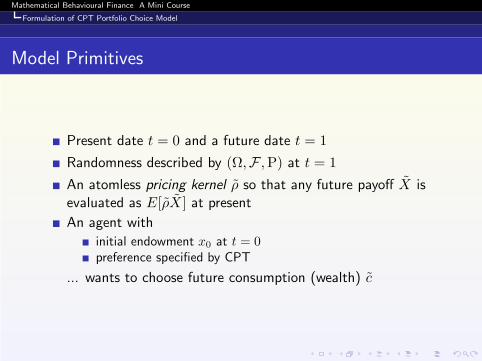
Model Primitives
Present date t = 0 and a future date t = 1
Randomness described by (Ω,F ,P) at t = 1
An atomless pricing kernel ρ so that any future payoff X isevaluated as E[ρX ] at present
An agent with
initial endowment x0 at t = 0preference specified by CPT
... wants to choose future consumption (wealth) c
Mathematical Behavioural Finance A Mini Course
Formulation of CPT Portfolio Choice Model
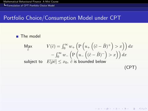
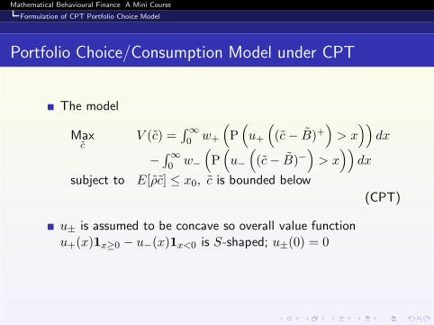
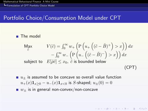
Portfolio Choice/Consumption Model under CPT
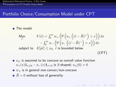
The model
Maxc
V (c) =∫∞
0 w+
(
P(
u+
(
(c− B)+)
> x))
dx
−∫∞
0 w−
(
P(
u−
(
(c− B)−)
> x))
dx
subject to E[ρc] ≤ x0, c is bounded below
(CPT)
Mathematical Behavioural Finance A Mini Course
Formulation of CPT Portfolio Choice Model
Portfolio Choice/Consumption Model under CPT
The model
Maxc
V (c) =∫∞
0 w+
(
P(
u+
(
(c− B)+)
> x))
dx
−∫∞
0 w−
(
P(
u−
(
(c− B)−)
> x))
dx
subject to E[ρc] ≤ x0, c is bounded below
(CPT)
u± is assumed to be concave so overall value functionu+(x)1x≥0 − u−(x)1x<0 is S-shaped; u±(0) = 0
w± is in general non-convex/non-concave
B = 0 without loss of generality

Mathematical Behavioural Finance A Mini Course
Formulation of CPT Portfolio Choice Model
CPT Preference
Write V (c) = V+(c+)− V−(c
−) where
V+(c) :=∫∞
0 w+ (P (u+ (c) > x)) dx
V−(c) :=∫∞
0 w− (P (u− (c) > x)) dx

Mathematical Behavioural Finance A Mini Course
Formulation of CPT Portfolio Choice Model
Mathematical Challenges
Two difference sources

Mathematical Behavioural Finance A Mini Course
Formulation of CPT Portfolio Choice Model
Mathematical Challenges
Two difference sources
Probability weighting and S-shaped value function

Mathematical Behavioural Finance A Mini Course
Formulation of CPT Portfolio Choice Model
Literature
Almost none

Mathematical Behavioural Finance A Mini Course
Formulation of CPT Portfolio Choice Model
Literature
Almost none
Berkelaar, Kouwenberg and Post (2004): no probabilityweighting; two-piece power value function
Mathematical Behavioural Finance A Mini Course
Formulation of CPT Portfolio Choice Model
Standing Assumptions
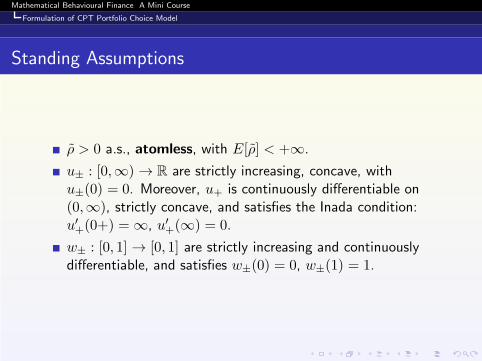
ρ > 0 a.s., atomless, with E[ρ] < +∞.
u± : [0,∞) → R are strictly increasing, concave, withu±(0) = 0. Moreover, u+ is continuously differentiable on(0,∞), strictly concave, and satisfies the Inada condition:u′+(0+) = ∞, u′+(∞) = 0.
w± : [0, 1] → [0, 1] are strictly increasing and continuouslydifferentiable, and satisfies w±(0) = 0, w±(1) = 1.

Mathematical Behavioural Finance A Mini Course
Divide and Conquer
Section 2
Divide and Conquer
Mathematical Behavioural Finance A Mini Course
Divide and Conquer
Our Model (Again)
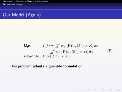
Maxc
V (c) =∫∞
0 w+ (P (u+(c+) > x)) dx
−∫∞
0 w− (P (u−(c−) > x)) dx
subject to E[ρc] ≤ x0, c ≥ 0
(P)
This problem admits a quantile formulation

Mathematical Behavioural Finance A Mini Course
Divide and Conquer
Divide and Conquer
We do “divide and conquer”

Mathematical Behavioural Finance A Mini Course
Divide and Conquer
Divide and Conquer
We do “divide and conquer”
Step 1: divide into two problems: one concerns the gain partof c and the other the loss part of c

Mathematical Behavioural Finance A Mini Course
Divide and Conquer
Divide and Conquer
We do “divide and conquer”
Step 1: divide into two problems: one concerns the gain partof c and the other the loss part of c
Step 2: combine them together via solving another problem
Mathematical Behavioural Finance A Mini Course
Divide and Conquer
Step 1 – Gain Part Problem (GPP)
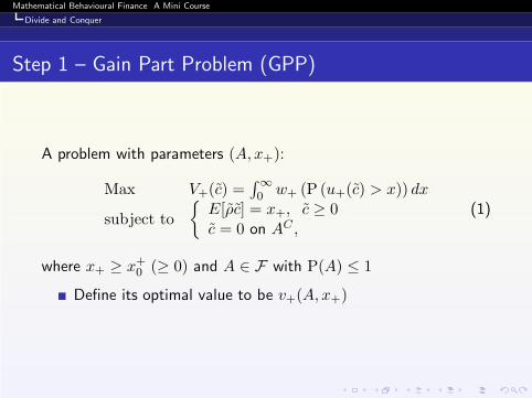
A problem with parameters (A, x+):
Max V+(c) =∫∞
0 w+ (P (u+(c) > x)) dx
subject to
E[ρc] = x+, c ≥ 0c = 0 on AC ,
(1)
where x+ ≥ x+0 (≥ 0) and A ∈ F with P(A) ≤ 1
Define its optimal value to be v+(A, x+)
Mathematical Behavioural Finance A Mini Course
Divide and Conquer
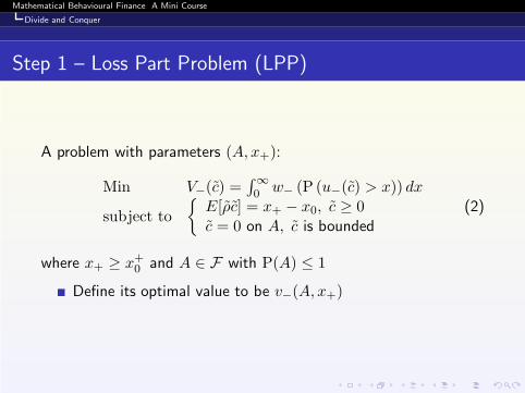
Step 1 – Loss Part Problem (LPP)
A problem with parameters (A, x+):
Min V−(c) =∫∞
0 w− (P (u−(c) > x)) dx
subject to
E[ρc] = x+ − x0, c ≥ 0c = 0 on A, c is bounded
(2)
where x+ ≥ x+0 and A ∈ F with P(A) ≤ 1
Define its optimal value to be v−(A, x+)

Mathematical Behavioural Finance A Mini Course
Divide and Conquer
Step 2
In Step 2 we solve
Max v+(A, x+)− v−(A, x+)
subject to
A ∈ F , x+ ≥ x+0 ,x+ = 0 when P(A) = 0,x+ = x0 when P(A) = 1.
(3)

Mathematical Behavioural Finance A Mini Course
Divide and Conquer
It Works
Theorem
(Jin and Zhou 2008) Given c∗, define A∗ := ω : c∗ ≥ 0 andx∗+ := E[ρ(c∗)+]. Then c∗ is optimal for the CPT portfolio choiceproblem (CPT) iff (A∗, x∗+) are optimal for Problem (3) and(X∗)+ and (X∗)− are respectively optimal for Problems (1) and(2) with parameters (A∗, x∗+).
Proof. Direct by definitions of maximum/minimum.

Mathematical Behavioural Finance A Mini Course
Divide and Conquer
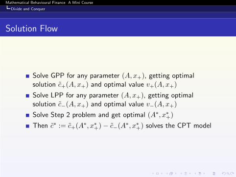
Solution Flow
Solve GPP for any parameter (A, x+), getting optimalsolution c+(A, x+) and optimal value v+(A, x+)

Mathematical Behavioural Finance A Mini Course
Divide and Conquer
Solution Flow
Solve GPP for any parameter (A, x+), getting optimalsolution c+(A, x+) and optimal value v+(A, x+)
Solve LPP for any parameter (A, x+), getting optimalsolution c−(A, x+) and optimal value v−(A, x+)

Mathematical Behavioural Finance A Mini Course
Divide and Conquer
Solution Flow
Solve GPP for any parameter (A, x+), getting optimalsolution c+(A, x+) and optimal value v+(A, x+)
Solve LPP for any parameter (A, x+), getting optimalsolution c−(A, x+) and optimal value v−(A, x+)
Solve Step 2 problem and get optimal (A∗, x∗+)
Then c∗ := c+(A∗, x∗+)− c−(A
∗, x∗+) solves the CPT model
Mathematical Behavioural Finance A Mini Course
Divide and Conquer
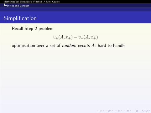
Simplification
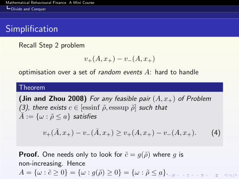
Recall Step 2 problem
v+(A, x+)− v−(A, x+)
optimisation over a set of random events A: hard to handle
Mathematical Behavioural Finance A Mini Course
Divide and Conquer
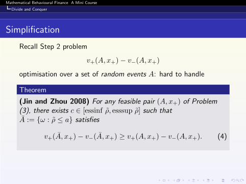
Simplification
Recall Step 2 problem
v+(A, x+)− v−(A, x+)
optimisation over a set of random events A: hard to handle
Theorem
(Jin and Zhou 2008) For any feasible pair (A, x+) of Problem(3), there exists c ∈ [essinf ρ, esssup ρ] such thatA := ω : ρ ≤ a satisfies
v+(A, x+)− v−(A, x+) ≥ v+(A, x+)− v−(A, x+). (4)
Mathematical Behavioural Finance A Mini Course
Divide and Conquer
Simplification
Recall Step 2 problem
v+(A, x+)− v−(A, x+)
optimisation over a set of random events A: hard to handle
Theorem
(Jin and Zhou 2008) For any feasible pair (A, x+) of Problem(3), there exists c ∈ [essinf ρ, esssup ρ] such thatA := ω : ρ ≤ a satisfies
v+(A, x+)− v−(A, x+) ≥ v+(A, x+)− v−(A, x+). (4)
Proof. One needs only to look for c = g(ρ) where g isnon-increasing. HenceA = ω : c ≥ 0 = ω : g(ρ) ≥ 0 = ω : ρ ≤ a.

Mathematical Behavioural Finance A Mini Course
Divide and Conquer
Step 2 Problem Rewritten
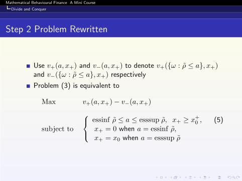
Use v+(a, x+) and v−(a, x+) to denote v+(ω : ρ ≤ a, x+)and v−(ω : ρ ≤ a, x+) respectively
Mathematical Behavioural Finance A Mini Course
Divide and Conquer
Step 2 Problem Rewritten
Use v+(a, x+) and v−(a, x+) to denote v+(ω : ρ ≤ a, x+)and v−(ω : ρ ≤ a, x+) respectively
Problem (3) is equivalent to
Max v+(a, x+)− v−(a, x+)
subject to
essinf ρ ≤ a ≤ esssup ρ, x+ ≥ x+0 ,x+ = 0 when a = essinf ρ,x+ = x0 when a = esssup ρ
(5)

Mathematical Behavioural Finance A Mini Course
Solutions to GPP and LPP
Section 3
Solutions to GPP and LPP
Mathematical Behavioural Finance A Mini Course
Solutions to GPP and LPP
GPP
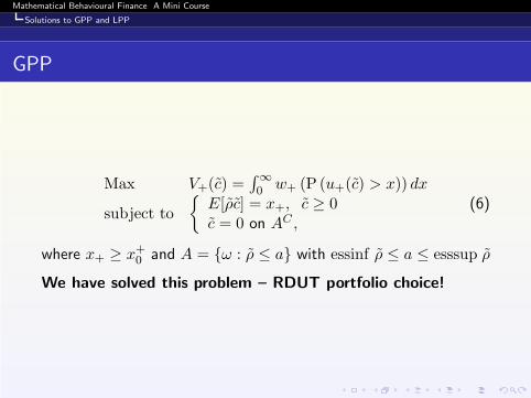
Max V+(c) =∫∞
0 w+ (P (u+(c) > x)) dx
subject to
E[ρc] = x+, c ≥ 0c = 0 on AC ,
(6)
where x+ ≥ x+0 and A = ω : ρ ≤ a with essinf ρ ≤ a ≤ esssup ρ
We have solved this problem – RDUT portfolio choice!

Mathematical Behavioural Finance A Mini Course
Solutions to GPP and LPP
Integrability Condition
Impose the intergrability condition
E
[
u+
(
(u′+)−1
(
ρ
w′+(Fρ(ρ))
))
w′+(Fρ(ρ))
]
< +∞

Mathematical Behavioural Finance A Mini Course
Solutions to GPP and LPP
Integrability Condition
Impose the intergrability condition
E
[
u+
(
(u′+)−1
(
ρ
w′+(Fρ(ρ))
))
w′+(Fρ(ρ))
]
< +∞
In the following, we always assume the integrability conditionholds
Mathematical Behavioural Finance A Mini Course
Solutions to GPP and LPP
Solutions to GPP
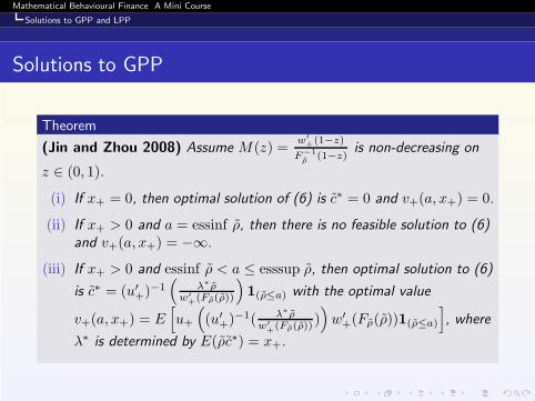
Theorem
(Jin and Zhou 2008) Assume M(z) =w′
+(1−z)
F−1ρ
(1−z)is non-decreasing on
z ∈ (0, 1).
(i) If x+ = 0, then optimal solution of (6) is c∗ = 0 and v+(a, x+) = 0.
(ii) If x+ > 0 and a = essinf ρ, then there is no feasible solution to (6)and v+(a, x+) = −∞.
(iii) If x+ > 0 and essinf ρ < a ≤ esssup ρ, then optimal solution to (6)
is c∗ = (u′+)
−1(
λ∗ρw′
+(Fρ(ρ))
)
1(ρ≤a) with the optimal value
v+(a, x+) = E[
u+
(
(u′+)
−1( λ∗ρ
w′
+(Fρ(ρ))))
w′+(Fρ(ρ))1(ρ≤a)
]
, where
λ∗ is determined by E(ρc∗) = x+.

Mathematical Behavioural Finance A Mini Course
Solutions to GPP and LPP
Idea of Proof
Work on conditional probability space(Ω ∩A,F ∩A,PA := P(·|A))

Mathematical Behavioural Finance A Mini Course
Solutions to GPP and LPP
Idea of Proof
Work on conditional probability space(Ω ∩A,F ∩A,PA := P(·|A))
Revise weighting function
wA(x) := w+(xP(A))/w+(P(A)), x ∈ [0, 1]

Mathematical Behavioural Finance A Mini Course
Solutions to GPP and LPP
Idea of Proof
Work on conditional probability space(Ω ∩A,F ∩A,PA := P(·|A))
Revise weighting function
wA(x) := w+(xP(A))/w+(P(A)), x ∈ [0, 1]
GPP is rewritten as
Max V+(c) = w+(P(A))∫∞
0 wA (PA (u+(c) > x)) dxsubject to
EA[ρc] = x+/P(A), c ≥ 0
Apply result in Chapter 2

Mathematical Behavioural Finance A Mini Course
Solutions to GPP and LPP
LPP
Min V−(c) =∫∞
0 w− (P (u−(c) > x)) dx
subject to
E[ρc] = x+ − x0, c ≥ 0c = 0 on A, c is bounded
(7)
where x+ ≥ x+0 and A = ω : ρ ≤ a with essinf ρ ≤ a ≤ esssup ρ
This is a minimisation problem!

Mathematical Behavioural Finance A Mini Course
Solutions to GPP and LPP
A General Problem
Minc
∫∞
0 w (P (u(c) > x)) dx
subject to E[ρc] ≥ x0, c ≥ 0(G)

Mathematical Behavioural Finance A Mini Course
Solutions to GPP and LPP
Hardy–Littlewood Inequality (Again)
Lemma
(Jin and Zhou 2008) We have that c∗ := G(Fρ(ρ)) solvesmaxc′∼cE [ρc′], where G is quantile of c. If in addition−∞ < E[ρc∗] < +∞, then c∗ is the unique optimal solution.
Hardy, Littlewood and Polya (1952), Dybvig (1988)

Mathematical Behavioural Finance A Mini Course
Solutions to GPP and LPP
Quantile Formulation
The quantile formulation of (G) is:
MinG∈G
U(G(·)) :=∫ 10 u(G(z))w′(1− z)dz
subject to∫ 10 F−1
ρ (z)G(z)dz ≥ x0(Q)

Mathematical Behavioural Finance A Mini Course
Solutions to GPP and LPP
Combinatorial Optimisation in Function Spaces
To minimise a concave functional: “wrong” direction!

Mathematical Behavioural Finance A Mini Course
Solutions to GPP and LPP
Combinatorial Optimisation in Function Spaces
To minimise a concave functional: “wrong” direction!
... which originates from S-shaped value function

Mathematical Behavioural Finance A Mini Course
Solutions to GPP and LPP
Combinatorial Optimisation in Function Spaces
To minimise a concave functional: “wrong” direction!
... which originates from S-shaped value function
Solution must have a very different structure compared withthe maximisation counterpart
Lagrange fails (positive duality gap)
Solution should be a “corner point solution”: essentially acombinatorial optimisation in an infinite dimensional space

Mathematical Behavioural Finance A Mini Course
Solutions to GPP and LPP
Characterising Corner Point Solutions
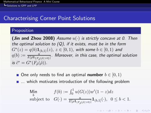
Proposition
(Jin and Zhou 2008) Assume u(·) is strictly concave at 0. Thenthe optimal solution to (Q), if it exists, must be in the formG∗(z) = q(b)1(b,1)(z), z ∈ [0, 1), with some b ∈ [0, 1) andq(b) := a
E[ρ1Fρ(ρ)>b]. Moreover, in this case, the optimal solution
is c∗ = G∗(Fρ(ρ)).
One only needs to find an optimal number b ∈ [0, 1)
Mathematical Behavioural Finance A Mini Course
Solutions to GPP and LPP
Characterising Corner Point Solutions
Proposition
(Jin and Zhou 2008) Assume u(·) is strictly concave at 0. Thenthe optimal solution to (Q), if it exists, must be in the formG∗(z) = q(b)1(b,1)(z), z ∈ [0, 1), with some b ∈ [0, 1) andq(b) := a
E[ρ1Fρ(ρ)>b]. Moreover, in this case, the optimal solution
is c∗ = G∗(Fρ(ρ)).
One only needs to find an optimal number b ∈ [0, 1)
... which motivates introduction of the following problem
Minb
f(b) :=∫ 10 u(G(z))w′(1− z)dz
subject to G(·) = aE[ρ1(Fρ(ρ)>b)]
1(b,1](·), 0 ≤ b < 1.

Mathematical Behavioural Finance A Mini Course
Solutions to GPP and LPP
Solving (G)
Theorem
(Jin and Zhou 2008) Assume u(·) is strictly concave at 0. Then(G) admits an optimal solution if and only if the following problem
min0≤b<esssup ρ
u
(
x0E[ρ1(ρ>b)]
)
w(P(ρ > b))
admits an optimal solution b∗, in which case the optimal solutionto (G) is c∗ = x0
E[ρ1(ρ>b∗)]1(ρ>b∗).
Mathematical Behavioural Finance A Mini Course
Solutions to GPP and LPP
Solutions to LPP
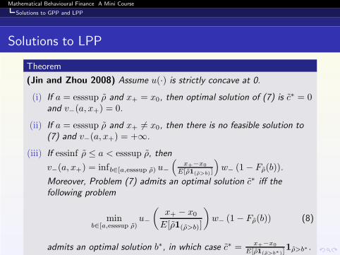
Theorem
(Jin and Zhou 2008) Assume u(·) is strictly concave at 0.
(i) If a = esssup ρ and x+ = x0, then optimal solution of (7) is c∗ = 0and v−(a, x+) = 0.
(ii) If a = esssup ρ and x+ 6= x0, then there is no feasible solution to(7) and v−(a, x+) = +∞.
(iii) If essinf ρ ≤ a < esssup ρ, then
v−(a, x+) = infb∈[a,esssup ρ) u−
(
x+−x0
E[ρ1(ρ>b)]
)
w− (1− Fρ(b)).
Moreover, Problem (7) admits an optimal solution c∗ iff thefollowing problem
minb∈[a,esssup ρ)
u−
(
x+ − x0
E[ρ1(ρ>b)]
)
w− (1− Fρ(b)) (8)
admits an optimal solution b∗, in which case c∗ = x+−x0
E[ρ1(ρ>b∗)]1ρ>b∗ .

Mathematical Behavioural Finance A Mini Course
Grand Solution
Section 4
Grand Solution

Mathematical Behavioural Finance A Mini Course
Grand Solution
A Mathematical Programme
Consider a mathematical programme in (a, x+):
Max(a,x+) E[
u+
(
(u′+)
−1(
λ(a,x+)ρw′
+(Fρ(ρ))
))
w′+(Fρ((ρ))1(ρ≤a)
]
−u−(x+−x0
E[ρ1ρ>a])w−(1 − F (a))
subject to
essinf ρ ≤ a ≤ esssup ρ, x+ ≥ x+0 ,
x+ = 0 when a = essinf ρ, x+ = x0 when a = esssup ρ),(MP)
where λ(a, x+) satisfies E[
(u′+)−1
(
λ(a,x+)ρw′
+(Fρ(ρ))
)
ρ1(ρ≤a)
]
= x+

Mathematical Behavioural Finance A Mini Course
Grand Solution
Grand Solution
Theorem
(Jin and Zhou 2008) Assume u−(·) is strictly concave at 0 andM is non-decreasing. Let (a∗, x∗+) solves (MP). Then the optimalsolution to (CPT) is
c∗ =
[
(u′+)
−1
(
λρ
w′+(Fρ(ρ))
)]
1(ρ≤a∗) −
[
x∗+ − x0
E[ρ1(ρ>a∗)]
]
1(ρ>a∗).
Mathematical Behavioural Finance A Mini Course
Grand Solution
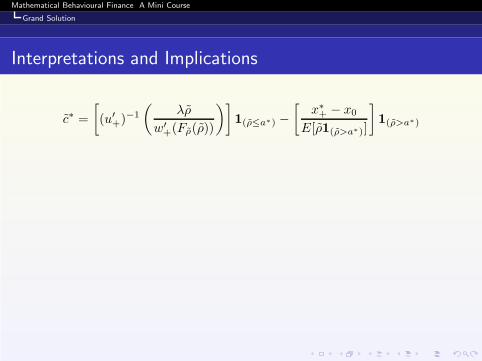
Interpretations and Implications
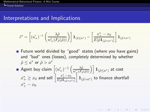
c∗ =
[
(u′+)
−1
(
λρ
w′+(Fρ(ρ))
)]
1(ρ≤a∗) −
[
x∗+ − x0
E[ρ1(ρ>a∗)]
]
1(ρ>a∗)
Mathematical Behavioural Finance A Mini Course
Grand Solution
Interpretations and Implications
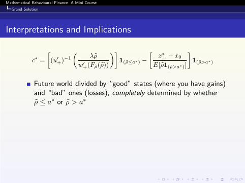
c∗ =
[
(u′+)
−1
(
λρ
w′+(Fρ(ρ))
)]
1(ρ≤a∗) −
[
x∗+ − x0
E[ρ1(ρ>a∗)]
]
1(ρ>a∗)
Future world divided by “good” states (where you have gains)and “bad” ones (losses), completely determined by whetherρ ≤ a∗ or ρ > a∗
Mathematical Behavioural Finance A Mini Course
Grand Solution
Interpretations and Implications
c∗ =
[
(u′+)
−1
(
λρ
w′+(Fρ(ρ))
)]
1(ρ≤a∗) −
[
x∗+ − x0
E[ρ1(ρ>a∗)]
]
1(ρ>a∗)
Future world divided by “good” states (where you have gains)and “bad” ones (losses), completely determined by whetherρ ≤ a∗ or ρ > a∗
Agent buy claim[
(u′+)−1
(
λρw′
+(Fρ(ρ))
)]
1(ρ≤a∗) at cost
x∗+ ≥ x0 and sell[
x∗+−x0
E[ρ1(ρ>a∗)]
]
1(ρ>a∗) to finance shortfall
x∗+ − x0
Mathematical Behavioural Finance A Mini Course
Grand Solution
Interpretations and Implications
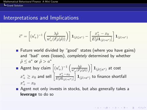
c∗ =
[
(u′+)
−1
(
λρ
w′+(Fρ(ρ))
)]
1(ρ≤a∗) −
[
x∗+ − x0
E[ρ1(ρ>a∗)]
]
1(ρ>a∗)
Future world divided by “good” states (where you have gains)and “bad” ones (losses), completely determined by whetherρ ≤ a∗ or ρ > a∗
Agent buy claim[
(u′+)−1
(
λρw′
+(Fρ(ρ))
)]
1(ρ≤a∗) at cost
x∗+ ≥ x0 and sell[
x∗+−x0
E[ρ1(ρ>a∗)]
]
1(ρ>a∗) to finance shortfall
x∗+ − x0Agent not only invests in stocks, but also generally takes aleverage to do so
Mathematical Behavioural Finance A Mini Course
Grand Solution
Interpretations and Implications
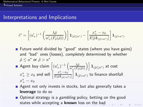
c∗ =
[
(u′+)
−1
(
λρ
w′+(Fρ(ρ))
)]
1(ρ≤a∗) −
[
x∗+ − x0
E[ρ1(ρ>a∗)]
]
1(ρ>a∗)
Future world divided by “good” states (where you have gains)and “bad” ones (losses), completely determined by whetherρ ≤ a∗ or ρ > a∗
Agent buy claim[
(u′+)−1
(
λρw′
+(Fρ(ρ))
)]
1(ρ≤a∗) at cost
x∗+ ≥ x0 and sell[
x∗+−x0
E[ρ1(ρ>a∗)]
]
1(ρ>a∗) to finance shortfall
x∗+ − x0Agent not only invests in stocks, but also generally takes aleverage to do so
Optimal strategy is a gambling policy, betting on the goodstates while accepting a known loss on the bad

Mathematical Behavioural Finance A Mini Course
Continuous Time and Time Inconsistency
Section 5
Continuous Time and Time Inconsistency
Mathematical Behavioural Finance A Mini Course
Continuous Time and Time Inconsistency
A Continuous-Time Economy
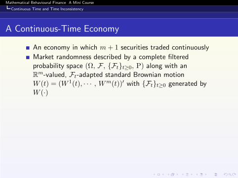
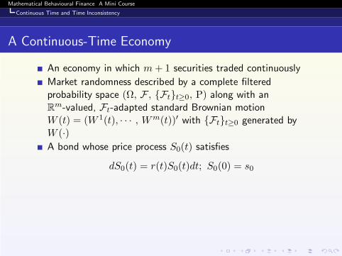
An economy in which m+ 1 securities traded continuously
Mathematical Behavioural Finance A Mini Course
Continuous Time and Time Inconsistency
A Continuous-Time Economy
An economy in which m+ 1 securities traded continuously
Market randomness described by a complete filteredprobability space (Ω, F , Ftt≥0, P) along with anRm-valued, Ft-adapted standard Brownian motion
W (t) = (W 1(t), · · · , Wm(t))′ with Ftt≥0 generated byW (·)
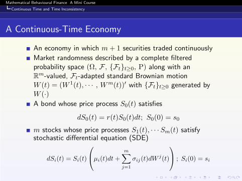
A bond whose price process S0(t) satisfies
dS0(t) = r(t)S0(t)dt; S0(0) = s0
Mathematical Behavioural Finance A Mini Course
Continuous Time and Time Inconsistency
A Continuous-Time Economy
An economy in which m+ 1 securities traded continuously
Market randomness described by a complete filteredprobability space (Ω, F , Ftt≥0, P) along with anRm-valued, Ft-adapted standard Brownian motion
W (t) = (W 1(t), · · · , Wm(t))′ with Ftt≥0 generated byW (·)
A bond whose price process S0(t) satisfies
dS0(t) = r(t)S0(t)dt; S0(0) = s0
m stocks whose price processes S1(t), · · · Sm(t) satisfystochastic differential equation (SDE)
dSi(t) = Si(t)
µi(t)dt+
m∑
j=1
σij(t)dWj(t)
; Si(0) = si

Mathematical Behavioural Finance A Mini Course
Continuous Time and Time Inconsistency
Tame Portfolios
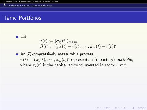
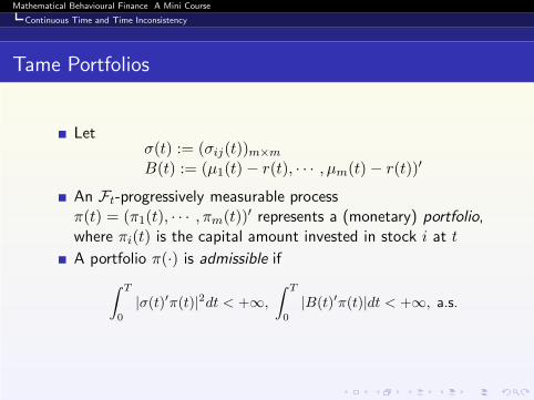
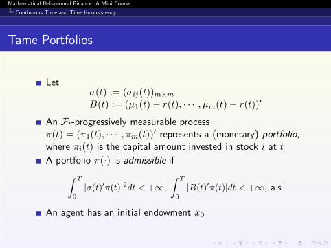
Letσ(t) := (σij(t))m×m
B(t) := (µ1(t)− r(t), · · · , µm(t)− r(t))′
Mathematical Behavioural Finance A Mini Course
Continuous Time and Time Inconsistency
Tame Portfolios
Letσ(t) := (σij(t))m×m
B(t) := (µ1(t)− r(t), · · · , µm(t)− r(t))′
An Ft-progressively measurable processπ(t) = (π1(t), · · · , πm(t))′ represents a (monetary) portfolio,where πi(t) is the capital amount invested in stock i at t
A portfolio π(·) is admissible if
∫ T
0
|σ(t)′π(t)|2dt < +∞,
∫ T
0
|B(t)′π(t)|dt < +∞, a.s.
An agent has an initial endowment x0
Mathematical Behavioural Finance A Mini Course
Continuous Time and Time Inconsistency
Wealth Equation
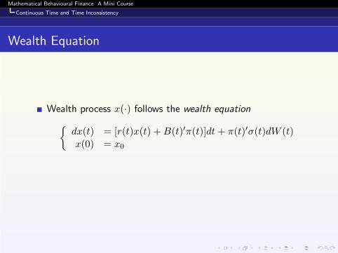
Wealth process x(·) follows the wealth equation
dx(t) = [r(t)x(t) +B(t)′π(t)]dt+ π(t)′σ(t)dW (t)x(0) = x0
Mathematical Behavioural Finance A Mini Course
Continuous Time and Time Inconsistency
Wealth Equation
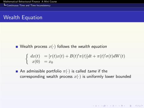
Wealth process x(·) follows the wealth equation
dx(t) = [r(t)x(t) +B(t)′π(t)]dt+ π(t)′σ(t)dW (t)x(0) = x0
An admissible portfolio π(·) is called tame if thecorresponding wealth process x(·) is uniformly lower bounded
Mathematical Behavioural Finance A Mini Course
Continuous Time and Time Inconsistency
Market Assumptions
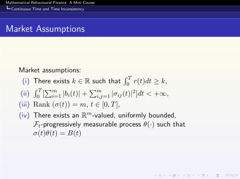
Market assumptions:
(i) There exists k ∈ R such that∫ T
0 r(t)dt ≥ k,
(ii)∫ T
0 [∑m
i=1 |bi(t)|+∑m
i,j=1 |σij(t)|2]dt < +∞,
(iii) Rank (σ(t)) = m, t ∈ [0, T ],
(iv) There exists an Rm-valued, uniformly bounded,
Ft-progressively measurable process θ(·) such thatσ(t)θ(t) = B(t)

Mathematical Behavioural Finance A Mini Course
Continuous Time and Time Inconsistency
Pricing Kernel
Define
ρ(t) := exp
−
∫ t
0
[
r(s) +1
2|θ(s)|2
]
ds−
∫ t
0
θ(s)′dW (s)

Mathematical Behavioural Finance A Mini Course
Continuous Time and Time Inconsistency
Pricing Kernel
Define
ρ(t) := exp
−
∫ t
0
[
r(s) +1
2|θ(s)|2
]
ds−
∫ t
0
θ(s)′dW (s)
Denote ρ := ρ(T )

Mathematical Behavioural Finance A Mini Course
Continuous Time and Time Inconsistency
Pricing Kernel
Define
ρ(t) := exp
−
∫ t
0
[
r(s) +1
2|θ(s)|2
]
ds−
∫ t
0
θ(s)′dW (s)
Denote ρ := ρ(T )
Assume that ρ is atomless

Mathematical Behavioural Finance A Mini Course
Continuous Time and Time Inconsistency
Continuous-Time Portfolio Choice under EUT
Max E[u(x(T ))]subject to (x(·), π(·)) : tame and admissible pair
(9)
where u is a concave utility function satisfying the usualassumptions

Mathematical Behavioural Finance A Mini Course
Continuous Time and Time Inconsistency
Forward Approach: Dynamic Programming
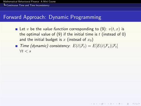
Let v be the value function corresponding to (9): v(t, x) isthe optimal value of (9) if the initial time is t (instead of 0)and the initial budget is x (instead of x0)
Mathematical Behavioural Finance A Mini Course
Continuous Time and Time Inconsistency
Forward Approach: Dynamic Programming
Let v be the value function corresponding to (9): v(t, x) isthe optimal value of (9) if the initial time is t (instead of 0)and the initial budget is x (instead of x0)
Time (dynamic) consistency: E(c|Ft) = E[E(c|Fs)|Ft]∀t < s
Mathematical Behavioural Finance A Mini Course
Continuous Time and Time Inconsistency
Forward Approach: Dynamic Programming
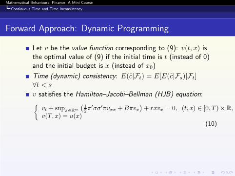
Let v be the value function corresponding to (9): v(t, x) isthe optimal value of (9) if the initial time is t (instead of 0)and the initial budget is x (instead of x0)
Time (dynamic) consistency: E(c|Ft) = E[E(c|Fs)|Ft]∀t < s
v satisfies the Hamilton–Jacobi–Bellman (HJB) equation:
vt + supπ∈Rm
(
12π
′σσ′πvxx +Bπvx)
+ rxvx = 0, (t, x) ∈ [0, T )× R,v(T, x) = u(x)
(10)
Mathematical Behavioural Finance A Mini Course
Continuous Time and Time Inconsistency
Forward Approach: Dynamic Programming
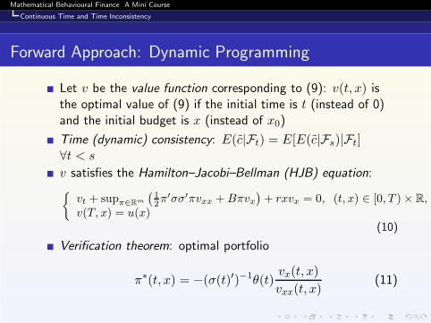
Let v be the value function corresponding to (9): v(t, x) isthe optimal value of (9) if the initial time is t (instead of 0)and the initial budget is x (instead of x0)
Time (dynamic) consistency: E(c|Ft) = E[E(c|Fs)|Ft]∀t < s
v satisfies the Hamilton–Jacobi–Bellman (HJB) equation:
vt + supπ∈Rm
(
12π
′σσ′πvxx +Bπvx)
+ rxvx = 0, (t, x) ∈ [0, T )× R,v(T, x) = u(x)
(10)
Verification theorem: optimal portfolio
π∗(t, x) = −(σ(t)′)−1θ(t)vx(t, x)
vxx(t, x)(11)
Mathematical Behavioural Finance A Mini Course
Continuous Time and Time Inconsistency
Backward Approach: Replication
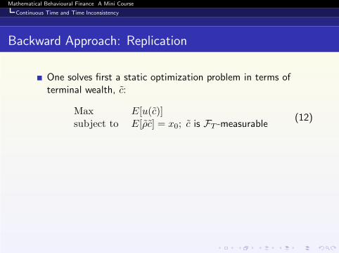
One solves first a static optimization problem in terms ofterminal wealth, c:
Max E[u(c)]subject to E[ρc] = x0; c is FT -measurable
(12)
Mathematical Behavioural Finance A Mini Course
Continuous Time and Time Inconsistency
Backward Approach: Replication
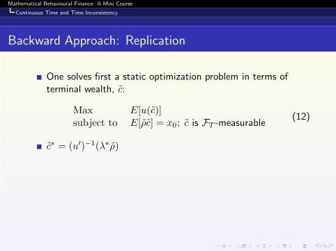
One solves first a static optimization problem in terms ofterminal wealth, c:
Max E[u(c)]subject to E[ρc] = x0; c is FT -measurable
(12)
c∗ = (u′)−1(λ∗ρ)
Mathematical Behavioural Finance A Mini Course
Continuous Time and Time Inconsistency
Backward Approach: Replication
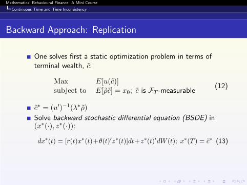
One solves first a static optimization problem in terms ofterminal wealth, c:
Max E[u(c)]subject to E[ρc] = x0; c is FT -measurable
(12)
c∗ = (u′)−1(λ∗ρ)
Solve backward stochastic differential equation (BSDE) in(x∗(·), z∗(·)):
dx∗(t) = [r(t)x∗(t)+θ(t)′z∗(t)]dt+z∗(t)′dW (t); x∗(T ) = c∗ (13)
Mathematical Behavioural Finance A Mini Course
Continuous Time and Time Inconsistency
Backward Approach: Replication
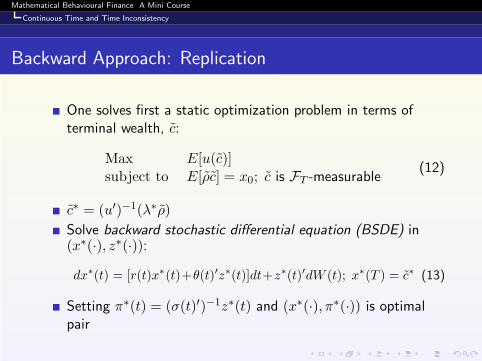
One solves first a static optimization problem in terms ofterminal wealth, c:
Max E[u(c)]subject to E[ρc] = x0; c is FT -measurable
(12)
c∗ = (u′)−1(λ∗ρ)
Solve backward stochastic differential equation (BSDE) in(x∗(·), z∗(·)):
dx∗(t) = [r(t)x∗(t)+θ(t)′z∗(t)]dt+z∗(t)′dW (t); x∗(T ) = c∗ (13)
Setting π∗(t) = (σ(t)′)−1z∗(t) and (x∗(·), π∗(·)) is optimalpair
Mathematical Behavioural Finance A Mini Course
Continuous Time and Time Inconsistency
Time Inconsistency under Probability Weighting
Choquet expectationE[X ] =
∫
Xd(w P) =∫∞
0 w(P(X > x))dx
Mathematical Behavioural Finance A Mini Course
Continuous Time and Time Inconsistency
Time Inconsistency under Probability Weighting
Choquet expectationE[X ] =
∫
Xd(w P) =∫∞
0 w(P(X > x))dx
How to define “conditional Choquet expectation”?
Mathematical Behavioural Finance A Mini Course
Continuous Time and Time Inconsistency
Time Inconsistency under Probability Weighting
Choquet expectationE[X ] =
∫
Xd(w P) =∫∞
0 w(P(X > x))dx
How to define “conditional Choquet expectation”?
Even if a conditional Choquet expectation can be defined, itwill not satisfy E(c|Ft) = E[E(c|Fs)|Ft]
Dynamic programming falls apart
Consider a weak notion of “optimality” - equilibrium portfolioin other settings (Ekeland and Pirvu 2008, Hu, Jin and Zhou2012, Bjork, Murgoci and Zhou 2012)

Mathematical Behavioural Finance A Mini Course
Continuous Time and Time Inconsistency
Replication: Pre-Committed Strategies
Solve a static optimisation problem (with probabilityweighting) in terms of terminal wealth

Mathematical Behavioural Finance A Mini Course
Continuous Time and Time Inconsistency
Replication: Pre-Committed Strategies
Solve a static optimisation problem (with probabilityweighting) in terms of terminal wealth
Such a problem has been solved by our approach developed
Mathematical Behavioural Finance A Mini Course
Continuous Time and Time Inconsistency
Replication: Pre-Committed Strategies
Solve a static optimisation problem (with probabilityweighting) in terms of terminal wealth
Such a problem has been solved by our approach developed
Find a dynamic portfolio replicating the obtained optimalterminal wealth
Such a portfolio is an optimal pre-committed strategy (Jinand Zhou 2008, He and Zhou 2011)

Mathematical Behavioural Finance A Mini Course
Summary and Further Readings
Section 6
Summary and Further Readings

Mathematical Behavioural Finance A Mini Course
Summary and Further Readings
Summary
Portfolio choice under CPT - probability weighting andS-shaped value function

Mathematical Behavioural Finance A Mini Course
Summary and Further Readings
Summary
Portfolio choice under CPT - probability weighting andS-shaped value function
Technical challenges

Mathematical Behavioural Finance A Mini Course
Summary and Further Readings
Summary
Portfolio choice under CPT - probability weighting andS-shaped value function
Technical challenges
Approach – divide and conquer

Mathematical Behavioural Finance A Mini Course
Summary and Further Readings
Summary
Portfolio choice under CPT - probability weighting andS-shaped value function
Technical challenges
Approach – divide and conquer
Combinatorial optimisation in infinte dimension

Mathematical Behavioural Finance A Mini Course
Summary and Further Readings
Summary
Portfolio choice under CPT - probability weighting andS-shaped value function
Technical challenges
Approach – divide and conquer
Combinatorial optimisation in infinte dimension
Optimal consumption profile markedly different from thatunder EUT – leverage and gambling behaviour
Inherent time inconsistency for continuous-time behaviouralproblems
Mathematical Behavioural Finance A Mini Course
Summary and Further Readings
Essential Readings
A. Berkelaar, R. Kouwenberg and T. Post. Optimal portfoliochoice under loss aversion, Review of Economics andStatistics, 86:973–987, 2004.
H. Jin and X. Zhou. Behavioral portfolio selection incontinuous time, Mathematical Finance, 18:385–426, 2008;Erratum, Mathematical Finance, 20:521–525, 2010.
Mathematical Behavioural Finance A Mini Course
Summary and Further Readings
Other Readings
T. Bjork, A. Murgoci and X. Zhou. Mean-variance portfolio optimization with state dependent riskaversion, Mathematical Finance, to appear; available at http://people.maths.ox.ac.uk/˜zhouxy/download/BMZ-Final.pdf
P. H. Dybvig. Distributional analysis of portfolio choice, Journal of Business, 61(3):369–398, 1988.
D. Denneberg. Non-Additive Measure and Integral, Kluwer, Dordrecht, 1994.
I. Ekeland and T. A. Pirvu. Investment and consumption without commitment, Mathematics and FinancialEconomics, 2:57–86, 2008.
G.H. Hardy, J. E. Littlewood and G. Polya. Inequalities, Cambridge University Press, Cambridge, 1952.
X. He and X. Zhou. Portfolio choice via quantiles, Mathematical Finance, 21:203–231, 2011.
Y. Hu, H. Jin and X. Zhou. Time-inconsistent stochastic linear-quadratic control, SIAM Journal onControl and Optimization, 50:1548–1572, 2012.
H. Jin, Z. Xu and X.Y. Zhou. A convex stochastic optimization problem arising from portfolio selection,Mathematical Finance, 81:171–183, 2008.
I. Karatzas and S. E. Shreve. Methods of Mathematical Finance, Springer, New York, 1998.

Mathematical Behavioural Finance A Mini Course
Final Words
Section 7
Final Words
Mathematical Behavioural Finance A Mini Course
Final Words
Two Revolutions in Finance
Finance ultimately deals with interplay between market riskand human judgement
Mathematical Behavioural Finance A Mini Course
Final Words
Two Revolutions in Finance
Finance ultimately deals with interplay between market riskand human judgement
History of financial theory over the last 50 years characterisedby two revolutions
Mathematical Behavioural Finance A Mini Course
Final Words
Two Revolutions in Finance
Finance ultimately deals with interplay between market riskand human judgement
History of financial theory over the last 50 years characterisedby two revolutions
Neoclassical (maximising) finance starting 1960s: Expectedutility maximisation, CAPM, efficient market theory, optionpricing
Mathematical Behavioural Finance A Mini Course
Final Words
Two Revolutions in Finance
Finance ultimately deals with interplay between market riskand human judgement
History of financial theory over the last 50 years characterisedby two revolutions
Neoclassical (maximising) finance starting 1960s: Expectedutility maximisation, CAPM, efficient market theory, optionpricingBehavioural finance starting 1980s: Cumulative prospecttheory, SP/A theory, regret and self-control, heuristics andbiases

Mathematical Behavioural Finance A Mini Course
Final Words
Neoclassical vs Behavioural
Neoclassical: the world and its participants are rational“wealth maximisers”

Mathematical Behavioural Finance A Mini Course
Final Words
Neoclassical vs Behavioural
Neoclassical: the world and its participants are rational“wealth maximisers”
Behavioural: emotion and psychology influence our decisionswhen faced with uncertainties, causing us to behave inunpredictable, inconsistent, incompetent, and most of all,irrational ways
A relatively new field that attempts to explain how and whyemotions and cognitive errors influence investors and createstock market anomalies such as bubbles and crashes

Mathematical Behavioural Finance A Mini Course
Final Words
Neoclassical vs Behavioural
Neoclassical: the world and its participants are rational“wealth maximisers”
Behavioural: emotion and psychology influence our decisionswhen faced with uncertainties, causing us to behave inunpredictable, inconsistent, incompetent, and most of all,irrational ways
A relatively new field that attempts to explain how and whyemotions and cognitive errors influence investors and createstock market anomalies such as bubbles and crashesIt seeks to explore the consistency and predictability in humanflaws so that such flaws can be avoided or even exploited forprofit

Mathematical Behavioural Finance A Mini Course
Final Words
Do We Need Both?
Foundations of the two
Mathematical Behavioural Finance A Mini Course
Final Words
Do We Need Both?
Foundations of the two
Neoclassical finance: Rationality (correct beliefs oninformation, risk aversion) – A normative theory

Mathematical Behavioural Finance A Mini Course
Final Words
Do We Need Both?
Foundations of the two
Neoclassical finance: Rationality (correct beliefs oninformation, risk aversion) – A normative theoryBehavioural finance: The lack thereof (experimental evidence,cognitive psychology) – A descriptive theory
Do we need both?

Mathematical Behavioural Finance A Mini Course
Final Words
Do We Need Both?
Foundations of the two
Neoclassical finance: Rationality (correct beliefs oninformation, risk aversion) – A normative theoryBehavioural finance: The lack thereof (experimental evidence,cognitive psychology) – A descriptive theory
Do we need both? Absolutely yes!
Neoclassical finance tells what people ought to do
Mathematical Behavioural Finance A Mini Course
Final Words
Do We Need Both?
Foundations of the two
Neoclassical finance: Rationality (correct beliefs oninformation, risk aversion) – A normative theoryBehavioural finance: The lack thereof (experimental evidence,cognitive psychology) – A descriptive theory
Do we need both? Absolutely yes!
Neoclassical finance tells what people ought to doBehavioural finance tells what people actually do
Mathematical Behavioural Finance A Mini Course
Final Words
Do We Need Both?
Foundations of the two
Neoclassical finance: Rationality (correct beliefs oninformation, risk aversion) – A normative theoryBehavioural finance: The lack thereof (experimental evidence,cognitive psychology) – A descriptive theory
Do we need both? Absolutely yes!
Neoclassical finance tells what people ought to doBehavioural finance tells what people actually doRobert Shiller (2006), “the two ... have always beeninterwined, and some of the most important applications oftheir insights will require the use of both approaches”
Mathematical Behavioural Finance A Mini Course
Final Words
Mathematical Behavioural Finance
“Mathematical behavioural finance” leads to new problems inmathematics and finance
Mathematical Behavioural Finance A Mini Course
Final Words
Mathematical Behavioural Finance
“Mathematical behavioural finance” leads to new problems inmathematics and finance
But ... is it justified: to rationally and mathematicallyaccount for irrationalities?
Mathematical Behavioural Finance A Mini Course
Final Words
Mathematical Behavioural Finance
“Mathematical behavioural finance” leads to new problems inmathematics and finance
But ... is it justified: to rationally and mathematicallyaccount for irrationalities?
Irrational behaviours are by no means random or arbitrary
“misguided behaviors ... are systamtic and predictable –making us predictably irrational” (Dan Ariely, PredictablyIrrational, Ariely 2008)
We use CPT/RDUT/SPA and specific value functions as thecarrier for exploring the “predictable irrationalities”
Mathematical behavioural finance: research is in its infancy,yet potential is unlimited – or so we believe