Mathematical finance - lecture notes(master course)

June 29, 2020

Abstract

These lecture notes build on the work of a number of different authors. Besides thebooks mentioned below we borrow extensively from lecture notes of Daniel Bartl andMichael Kupper.

1 Martingales and Arbitrage theory in discrete time

Throughout this section we fix a stochastic basis (Ω,F ,P, (Ft)Tt=0). X = (Xt)Tt=0 will denote an

adapted process. We shall also assume that F0 = ∅,Ω,FT = F .We will use the process X as a model for the asset price. Specifically, the random variable

Xt denotes the price of the asset under consideration at time t.Trades in the asset are modelled through predictable processes. We thus make the following

definitions:

Definition 1.1. A process H = (Ht)Tt=1 is called predictable or a trading strategy if Ht is

Ft−1-measurable for t = 1, . . . , T .

The economic interpretation of a trading strategy H = (Ht)Tt=1 is that Ht denotes the number

of shares that we own from time t− 1 to time t. As usual the σ-algebra Ft models the amount ofinformation available at time t. The assumption that Ht should be Ft−1-measurable correspondsto the fact that we can use only information available at time t − 1 to determine how manyshares we want to buy at time t− 1.

If we own Ht shares from time t− 1 to time t our wealth changes by

Ht(Xt −Xt−1).

Of course such changes in our wealth accumulate over time. This leads to the following

1

Definition 1.2. Let H be a trading strategy. The wealth process / value process / gains fromtrading process is given by

Vt := (H ·X)t :=t∑

k=1

Hk(Xk −Xk−1). (1.1)

We write S for the set of all values that can be achieved by trading in X wrt a bounded strategy,i.e.

S := (H ·X)T : H predictable and bounded..

A fundamental assumption for models of financial markets is that they do not allow forriskless profits, so called arbitrage opportunities.

Definition 1.3. A trading strategy H is an arbitrage opportunity if

P((H ·X)T ≥ 0) = 1, P((H ·X)T > 0) > 0.

We say that a market satisfies the no arbitrage assumption (NA) if there exists no boundedarbitrage strategy.

Remark 1.4. Assume that Q is another measure on (Ω,F) which is equivalent to P. Then Xsatisfies (NA) wrt P iff it satisfies (NA) wrt Q.

The following result justifies the restriction to bounded trading strategies. Moreover it yieldsthat the arbitrage can be looked in already in one period.

Proposition 1.5. The following are equivalent:

(i) There exists an arbitrage opportunity.

(ii) There exists t ∈ 1, . . . , T and η ∈ L0(Ft−1;Rd) such that

η · (Xt −Xt−1) ≥ 0 P-a.s. and

P(η · (Xt −Xt−1) > 0) > 0.(1.2)

(iii) There exists t ∈ 1, . . . , T and η ∈ L∞(Ft−1;Rd) satisfying (1.2).

(iv) There exists a bounded arbitrage opportunity.

Proof.

(a) We show that (i) implies (ii). Let H be an arbitrage opportunity with gains processVt = (H ·X)t. Define

t := infk ∈ 0, . . . , T : Vk ≥ 0 P-as and P(Vk > 0) > 0.

2

By assumption, t ≤ T and either Vt−1 = 0 or P(Vt−1 < 0) > 0. If Vt−1 = 0 then

Ht · (Xt −Xt−1) = Vt − Vt−1 = Vt

so that η := Ht satisfies (1.2). If P(Vt−1 < 0) > 0, define η := Ht11Vt−1<0, which isFt−1-measurable. Hence,

η · (Xt −Xt−1) = (Vt − Vt−1)11Vt−1<0 ≥ −Vt−111Vt−1<0

which shows that η satisfies (1.2).

(b) We show that (ii) implies (iii). Fix η ∈ L0(Ft−1) such that (1.2) holds. Since P(⋃c∈N|η| ≤

c) = 1, continuity of P implies

P (η · (Xt −Xt−1) > 0, |η| ≤ c) > 0

for some c > 0. But then η11|η|≤c ∈ L∞(Ft−1) satisfies (1.2).

(c) Suppose that (iii) holds, i.e. there exists t ∈ 1, . . . , T and η ∈ L∞(Ft−1) such that (1.2)holds. Then

Hs :=

η, s = t,

0, s 6= t.

defines a bounded arbitrage strategy.

(d) It remains to show that (iv) implies (i), but this is obvious.

A first goal of this lecture is to understand what type of models satisfy NA. The answer istightly linked to the concept of martingales:

Definition 1.6. Assume that X is an integrable process. X is a martingale if for 0 ≤ s ≤ t ≤ T

E[Xt|Fs] = Xs.

X is called sub-martingale if E[Xt|Fs] ≥ Xs for all 0 ≤ s ≤ t ≤ T . X is called super-martingaleif E[Xt|Fs] ≤ Xs for all 0 ≤ s ≤ t ≤ T .

A probability measure Q on (Ω,F) is called martingale measure (for X) if X is a Q-martingale, i.e. if EQ[Xt|Fs] = Xs for all 0 ≤ s ≤ t ≤ T .

If furthermore, Q ∼ P, Q is called an equivalent martingale measure. The set of all equivalentmartingale measures will be denoted by M.

Apparently X is a martingale if E[Xn|Fn−1] = Xn−1 for n = 1, . . . , T .

3

Lemma 1.7. If H is a bounded trading strategy and X is a martingale, then the process((H ·X)t)

Tt=0 is a martingale as well.

X is a martingale iff E(H ·X)T = 0 for all bounded trading strategies H.

Proof. Exercise.

Theorem 1.8. For a probability measure Q on (Ω,F) with Q P, the following are equivalent:

(i) The measure Q is a martingale measure.

(ii) Whenever H is a bounded trading strategy, then EQ(H ·X) = 0.

(iii) Whenever H is a bounded trading strategy, then the corresponding gains process (H ·X) isa Q-martingale.

(iv) Whenever H is a trading strategy such that EQ[(H ·X)−T ] < ∞, then the correspondinggains process (H ·X) is a Q-martingale (and in particular, (H ·X)T is Q-integrable).

Proof. The first equivalences are a simple consequence of Lemma 1.7. To establish (iv) istechnically more subtle and we refer the reader to [3].

Lemma 1.9. If X is a martingale, then X satisfies NA. More generally, if there exists anequivalent martingale measure for X, then X satisfies NA.

Proof. Exercise.

1.1 The Fundamental Theorem of Asset Pricing (FTAP)

Remarkably the converse of Lemma 1.9 is true as well:

Theorem 1.10. Assume that X satisfies (NA). Then there exists an equivalent probabilitymeasure Q ∼ P such that Xt ∈ L1(Q) and X is a Q-martingale.

In fact Theorem 1.10 is a relatively non trivial result first proved by Dalang, Morton andWillinger [1]. Typical approaches to this result require a non negligible amount of functionalanalysis. We refer to [2] for a modern account. Here we will content ourselves with a proofunder the additional assumption that Ω has only finitely many elements.

Assume from now until the end of Section 1.1 that we work under the following

Assumption 1.11. Assume that Ω = ω1, . . . , ωN, where ωi 6= ωj for i 6= j and that P(ω) >0 for all ω ∈ Ω. Moreover we assume that FT = F is the power set of Ω and that F0 = ∅,Ω.

4

It follows that all random variables on Ω are bounded and hence the vector space of allrandom variables consists of

V := L∞ := L∞(P).

Moreover, making the identification 1ωi = (0, . . . , 0︸ ︷︷ ︸i−1

, 1, 0, . . . , 0︸ ︷︷ ︸N−i

) we find that V ∼= RN . The dual

space V d is of course again isomorphic to RN . In the present context, it can also be identifiedwith L1 := L1(Ω), or, more importantly with the vector space SM of all signed measures on Ω.Specifically, any linear functional on V is given by a mapping

Z 7→ 〈Z, σ〉 :=

∫Z dσ,

for a signed measure σ ∈ SM.We also write L+ for the cone of all non-negative random variables and SM+ for the cone

of non-negative measures.In the proof of Theorem 1.10 we will need the following version of the Hahn-Banach theorem:

Theorem 1.12. Assume that A,B ⊆ RN are closed convex sets and that B is compact. Thenthere exist y ∈ (RN)d and α, β ∈ R such that

∀a ∈ A, b ∈ B, 〈a, y〉 ≤ α < β ≤ 〈b, y〉.

If A is a subspace, then 〈a, y〉 = 0 for all a ∈ A and in particular one can choose α = 0.

Proof of Theorem 1.10. (NA) is equivalent to S ∩ L+ = 0. Denoting

B :=

N∑i=1

λi1ωi :N∑i=1

λi = 1, λi ≥ 0

,

we thus haveB ∩ S = 0.

By Theorem 1.12 applied to the subspace S and the convex compact set B, there exists σ ∈ SM+

such that∀G ∈ S,∀X ∈ B, 〈G, σ〉 ≤ 0 < 〈X, σ〉.

Since σ(ω) = 〈1ω, σ〉 > 0 for ω ∈ Ω, we have that σ is a positive measure and in fact σ ∼ P.Setting Q := σ/σ(Ω) we obtain a probability measure satisfying Q ∼ P.

Since S is a subspace, we have for G ∈ S, 〈G, σ〉 = 0, hence also 0 = 〈G,Q〉 = EQ[G]. ByLemma 1.7 this yields that Q is a martingale measure as desired.

5

1.2 European contingent claims

Throughout this section we assume that there is an equivalent martingale measure, i.e. M 6= ∅.

Definition 1.13. A non-negative random variable C on (Ω,F ,P) is called a European contingentclaim. A European contingent claim is called a derivative of the underlying asset X if C ismeasurable with respect to σ(X) = σ(X0, . . . , XT ).

Remark 1.14. By a basic result of measure theory, a contingent claim C is a derivative of Xiff there exists a Borel-measurable function f ≥ 0 such that C = f(X0, . . . , XT ).

Remark 1.15. A European contingent claim has the interpretation of an asset which yields attime T the amount C, depending on the scenario of the market evolution. Here, T is called theexpiration date or the maturity of C.

Example 1.16.

(i) European call option: Ccall = (XT −K)+. The owner of a European call option has theright but not the obligation to buy the asset i at time T for a fixed strike price K.

(ii) European put option: Cput = (K −XT )+. The owner of an European put option has theright but not the obligation to sell the asset i at time T for a fixed strike price K.

(iii) Path dependent contingent claim, e.g. up-and-out call:

Ccallu&o =

(XT −K)+, maxt∈0,...,TXt < B,

0, otherwise.

Definition 1.17. A contingent claim C is called attainable (replicable) if there exist a ∈ Rand a trading strategy H such that a + (H · X)T = C P-a.s. In this case (a,H) is called areplicating strategy. The value a is interpreted as the initial capital / initial endowment andVt := a+ (H ·X)t is the corresponding value process.

Remark 1.18. The concept of replication plays a central role in mathematical finance.Let C be a contingent claim with replicating strategy (a,H), i.e. C = a + (H · X)T . We

assume that a rational financial agent is able to figure out such a trading strategy. But thisimplies that she should be indifferent between owning the claim C and the initial capital a: Ifshe owns a Euros at initial time and would like to switch this for a payoff C at the terminaltime T , all she has to do is to invest in the market according to the strategy H.

In this sense a is the ‘fair value’ or ‘fair price’ of the contingent claim C.If there exists a strategy H such that C = (H · X)T , then we say that C is attainable at

price 0. We denote byS := (H ·X)T : H predictable

the set of all claims that are attainable at price 0.

6

Theorem 1.19. Let C be an attainable claim. Then EQ[C] <∞ for every Q ∈M. The valueprocess of any replicating strategy (a,H) satisfies Vt = EQ[C|Ft] P-a.s. for all t ∈ 0, . . . , Tand Q ∈ M. In particular, the value process V is an M-martingale, i.e. a Q-martingale forevery Q ∈M.

Proof. Let Vt = a+ (H ·X)t be the value process to the trading strategy H with VT = C ≥ 0.Theorem 1.8 shows that for every Q ∈ M the value process V is a Q-martingale, that isVt = EQ[VT |Ft] P-a.s. for every t ∈ 0, . . . , T. In particular, EQ[C] = EQ[VT ] = V0 ∈ R.

The proof of Theorem 1.19 is more subtle than it might seem: to be able to apply Theorem1.8 it was necessary to guarantee some integrability of the negative part which is the reasonfor making our standing assumption that European contingent claims are non negative. (Ofcourse this assumption is met in all practical instances.) Clearly we do not need to care forsuch subtleties under the simplifying Assumption 1.11.

Remark 1.20. In the setup of Theorem 1.19 we have:

(i) The value process V does not depend on the replicating strategy (a,H).

(ii) We have EQ1 [VT |Ft] = EQ2 [VT |Ft] P-a.s. for all Q1,Q2 ∈M.

1.3 Complete markets

Definition 1.21. An arbitrage-free market model is called complete, if every contingent claimis attainable.

Apparently, complete market models are particularly convenient from a theoretical perspec-tive. In fact, complete markets are most commonly used in practice for their simplicity (eventhough this condition is not met in reality).

The following result characterises completeness in terms of martingale measures. (It is thusanalogous to the FTAP which characterises absence of arbitrage in terms of martingales.)

Theorem 1.22 (Second fundamental theorem of asset pricing). An arbitrage-free market modelis complete if and only if |M| = 1.

As in the case of the first FTAP, one direction of the proof is (essentially) trivial:

Proof of Theorem 1.22, easy part. If the market is complete, then for every A ∈ FT , the con-tingent claim C := 11A is attainable. By Theorem 1.19, the function

M→ [0, 1], Q 7→ EQ[11A] = Q(A)

is constant so that |M| = 1.

7

For the converse direction, we work again under the simplifying Assumption 1.11. In a firststep we provide an analogue of Lemma 1.7. While Lemma 1.7 characterizes martingales interms of trading strategies, we now establish that trading strategies can be characterized interms of martingales.

Recall that S denotes the set of all claims that are attainable at price 0. The followinglemma provides a fundamental characterization of S in terms of martingale measures.

Lemma 1.23. Assume that the market model satisfies NA. Let Z be a bounded random variablesuch that EQ[Z] = 0 for every martingale measure Q. Then Z ∈ S, i.e. there exists a tradingstrategy H such that (H ·X)T = Z.

Proof. Given a vector space W with dual space W d and K ⊆ W we write

K⊥ = y ∈ W d : 〈x, y〉 = 0 for all x ∈ K.

Denote the linear space generated by a subset K of W by span(K). Assuming that W is finitedimensional, it is well known from linear algebra that (K⊥)⊥ = span(K). (In fact this is asimple consequence of the Hahn-Banach theorem.)

Recall that S = (H ·X)T : H is a trading strategy and that SM,SM+ denote the sets ofsigned and non negative measures on Ω, respectively. We write SM++ for the set of all ‘strictlypostive’ measures, i.e. non-negative measures that are equivalent to P.

We claim that

span(S⊥ ∩ SM++) = S⊥. (1.3)

Since S⊥ is a subspace, the inclusion span(S⊥ ∩ SM++) ⊆ S⊥ is trivial.To prove the converse assume that σ ∈ S⊥. Let Q be an equivalent martingale measure and

recall that Q ∈ S⊥. Pick α ∈ R+ such that σ + αQ ∈ SM++. Then we also have σ + αQ ∈S⊥ ∩ SM++. Since Q itself is also an element of S⊥ ∩ SM++, we have σ ∈ span(S⊥ ∩ SM++),establishing (1.3).

Assume now that EQ[Z] = 0 for all equivalent martingale measures Q. Then we also haveEσ[Z] = 0 for all σ ∈ S⊥ ∩ SM++, hence

Z ∈ (S⊥ ∩ SM++)⊥ = (S⊥)⊥ = S.

Proof of Theorem 1.22, interesting part. Write Q for the unique equivalent martingale measureand let C be a contingent claim. We need to prove that C is attainable.

Set a := EQC. Then, trivially,EQ(C − a) = 0

for all equivalent martingale measures Q. By Lemma 1.23 there is a trading strategy H suchthat C − a = (H ·X)T . Hence (a,H) is a replicating strategy for C.

8

The following result is important in view of our subsequent development of the theory ofderivative pricing in continuous time.

Theorem 1.24 (Martingale representation theorem). For Q ∈M, the following statements areequivalent:

(i) We have M = Q (the market is complete).

(ii) Every Q-martingale M has the representation

Mt = M0 +t∑

k=1

Hk · (Xk −Xk−1)

for some predictable process H.

Proof. Exercise.

1.4 Pricing by no arbitrage

We extend our previous definition of arbitrage to a market which contains a financial derivative.The purpose is to define the notion of ‘arbitrage free price’.

During the entire section we assume that the market model is free of arbitrage.

Definition 1.25. Let C be a financial derivative and πC ∈ R. We say that the price πC

introduces arbitrage if there exist α ∈ R and a trading strategy H such that

P((H ·X)T + α(C − πC) ≥ 0) = 1, P((H ·X)T + α(C − πC) > 0) > 0.

Otherwise we call πC an arbitrage free price.

Remark 1.26. If C is attainable through a strategy (a,H) then a is the unique arbitrage freeprice.

Proof. Exercise.

Theorem 1.27. The set of arbitrage-free prices of a claim C is non-empty and given by

Π(C) = EQ[C] : Q ∈M such that EQ[C] <∞.

Proof. We refer to [3] for a proof. Under the simplifying Assumption 1.11 it is a relativelystraight forward application of Lemma 1.23

9

2 Brownian Motion and foundations of stochastic anal-

ysis

Brownian motion is the most important stochastic process in continuous time. It will serve asthe fundamental building block of all continuous time models considered in this lecture. In thissection we sketch its construction and some of its basic properties.

Throughout this section (Ω,F ,P, (Ft)t≥0) denotes a filtered probability space in continuoustime. Whenever we consider a stochastic process, we implicitly assume that it is adapted wrt.this basis. We will also need that (Ω,F ,P) is rich enough to support a RV X that is continuouslydistributed (i.e. P(X = a) = 0 for all a ∈ R).

2.1 Construction of (pre) Brownian motion

Definition 2.1. A process B = (Bt)t≥0 is called a (standard) Brownian motion if it satisfiesthe following:

1. ‘start in 0’: B0 = 0.

2. ‘Gaussian increments’: for 0 ≤ s ≤ t we have Bt −Bs ∼ N(0, t− s).

3. ‘independent increments’: given t0 ≤ . . . ≤ tn, the increments Bt1 −Bt0 , . . . , Btn −Btn−1

are independent.

4. ‘continuous paths’: for almost all ω the path t 7→ Bt(0) is continuous.

If the process B satisfies only properties (1)-(3), then B is called a pre Brownian motion.

A process that satisfies (4) is called a continuous process.If instead of (1) we have that B0 ∼ a, a ∈ R, we say that B is a Brownian motion started in

a. More generally, if Y is a random variable independent of (Bt − B0) for t ≥ 0 and B0 = Ythen we say that B is a Brownian motion started in Y .

If B is a Brownian motion and Bt −Bs is independent of Fs for 0 ≤ s ≤ t, then we say thatB is a Brownian motion wrt. (Ft)t≥0. This property is satisfied automatically if we take (Ft)t≥0

to be the filtration generated by B. (Warning: It is often assumed that B is a Brownian motionwrt. the underlying filtration without making this point explicit.)

Next we sketch the proof that a Brownian motion exists. Our starting point is the followingalternative characterization of a pre Brownian motion:

Lemma 2.2. A stochastic process is a pre Brownian motion iff it satisfies

1. B0 = 0.

2. E[BsBt] = s ∧ t for 0 ≤ s ≤ t.

10

3. For all t0 ≤ . . . ≤ tn, (Bt0 , . . . , Btn) is centered Gaussian.

Proof. Exercise using the properties of Gaussian RV.

An important point of this characterisation is that properties (1) and (2) are properties ofthe Hilbert space L2(Ω,P): (1) asserts that ‖B0‖1 = 0, (2) is equivalent to 〈Bs, Bt〉 = s ∧ t.

We also make the important comment that one can easily find an example of a Hilbert spaceand a family of elements, such that these properties are satisfied: Indeed we can just take

V = L2(R+, λ), ft := 1[0,t), t ≥ 0. (2.1)

Then V is a Hilbert space, ‖f0‖0 = 0, and

〈fs, ft〉 =

∫1[0,s)1[0,t) dλ = s ∧ t.

The idea behind our construction of a pre Brownian motion is to embed this space V into a‘large’ space consisting entirely of Gaussian random variables. To formalize this, we start withthe following definition.

Definition 2.3. A Gaussian space is a closed subspace Γ ⊆ L2(Ω,P) such that (X0, . . . , Xn) iscentered Gaussian for all X1, . . . , Xn ∈ Γ.

Lemma 2.4. If (Ω,F ,P) is rich enough to support a RV X that is continuously distributed,then L2(Ω,P) contains an infinite dimensional Gaussian space.

Sketch of proof. It is not hard to see that (Ω,F ,P) also supports a sequence X1, X2, . . . of iidRV satisfying Xi ∼ N(0, 1), i ≥ 1. It then can be shown (using properties of multivariateGaussians) that the closed spaced generated by X1, X2, . . . is Gaussian.

Using the above ingredients, we can now establish the existence of a pre Brownian motion.

Theorem 2.5. There exists a pre Brownian motion.

Proof. Let Γ ⊆ L2(Ω,P) be an infinite dimensional Gaussian space. Let V, (ft)t≥0 be as in (2.1).Since V is a separable Hilbertspace, there exists an isometry φ which embeds V into Γ. SetBt = φ(ft) for t ≥ 0. Then ‖B0‖0 = 0 and

E[BsBt] = 〈fs, ft〉 = s ∧ t

for 0 ≤ s ≤ t. Hence B = (Bt)t≥0 is a pre Brownian motion.

Naturally we could hope that every pre Brownian motion automatically has continuouspaths. This is not the case. Indeed, if B is a Brownian motion satisfying then there exists aprocess B = (Bt)t≥0 satisfying Bt = Bt, P-a.s. for every t such that the path t 7→ Bt(ω) is notcontinuous for every ω ∈ Ω. However, B is still a pre Brownian motion. In fact the process Bcan even be chosen in such a way that tωBt(ω) is P-a.s. nowhere continuous.

These considerations motivate the following notions of ‘similarity’ for stochastic processes.

11

Definition 2.6. Let X = (Xt)t≥0 and X ′ = (X ′t)t≥0 be stochastic processes on a stochastic basis(Ω,F ,P, (Ft)g≥0).

X and X ′ are indistinguishable if there exists a (measurable) set Ω1,P(Ω1) = 1 such that

Xt(ω) = X ′t(ω) for all ω ∈ Ω1, t ≥ 0.

X and X ′ are modifications (of each other) if

Xt(ω) = X ′t(ω) P-a.s. for all t ≥ 0.

Let X = (Xt)t≥0 and X ′ = (X ′t)t≥0 be stochastic processes defined on stochastic bases(Ω,F ,P, (Ft)g≥0) and (Ω′,F ′,P′, (F ′t)g≥0), resp. Then X is a version of X ′ if X and X ′ havethe same finite dimensional distributions.

Apparently ‘indistinguishabilty’ is stronger than ‘being modifications’ which in turn isstronger than ‘being versions’. If process X, X ′ are indistinguishable and X is continuous, thenX ′ is continuous as well. In contrast, the modification of a continuous process is not continuousin general.

Notably the notions of modification and indistinguishability coincide for continuous processes:

Proposition 2.7. Assume that X,X ′ are continuous processes that are modifications of eachother. Then X and X ′ are indistinguishable.

Proof. Exercise.

The notion of ‘version’ allows us to formalize a uniqueness property of (pre) Brownianmotion:

Proposition 2.8 (Uniqueness of pre Brownian motion). Assume that B,B′ are Brownianmotions (potentially) on different probability spaces. Then B is a version of B′.

Proof. Exercise.

The final step of constructing a Brownian motion will consist in defining an adequatemodification of a pre Brownian motion which does have continuous paths.

2.2 The Kolmogorov continuity theorem - final step of constructionof Brownian motion

The Kolmogorov extension theorem is a very useful tool, since it provides existence results forstochastic processes.

Definition 2.9. A function f : [0,∞)→ Rd is Holder continuous with exponent γ > 0, if thereexists a constant c > 0 such that |f(t)− f(s)| ≤ c|t− s|γ for all s, t ∈ [0,∞).

12

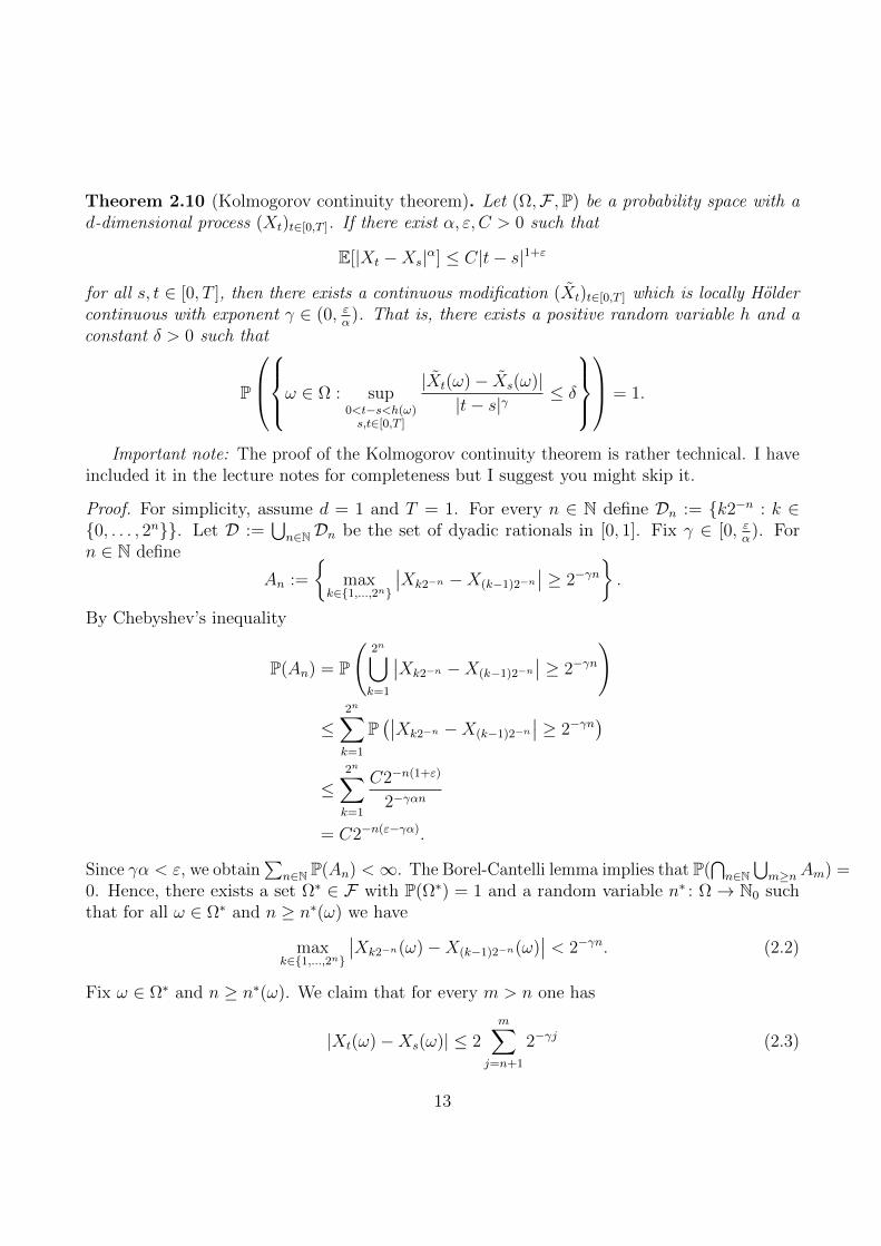
Theorem 2.10 (Kolmogorov continuity theorem). Let (Ω,F ,P) be a probability space with ad-dimensional process (Xt)t∈[0,T ]. If there exist α, ε, C > 0 such that

E[|Xt −Xs|α] ≤ C|t− s|1+ε

for all s, t ∈ [0, T ], then there exists a continuous modification (Xt)t∈[0,T ] which is locally Holdercontinuous with exponent γ ∈ (0, ε

α). That is, there exists a positive random variable h and a

constant δ > 0 such that

P

ω ∈ Ω : sup

0<t−s<h(ω)s,t∈[0,T ]

|Xt(ω)− Xs(ω)||t− s|γ

≤ δ

= 1.

Important note: The proof of the Kolmogorov continuity theorem is rather technical. I haveincluded it in the lecture notes for completeness but I suggest you might skip it.

Proof. For simplicity, assume d = 1 and T = 1. For every n ∈ N define Dn := k2−n : k ∈0, . . . , 2n. Let D :=

⋃n∈NDn be the set of dyadic rationals in [0, 1]. Fix γ ∈ [0, ε

α). For

n ∈ N define

An :=

max

k∈1,...,2n

∣∣Xk2−n −X(k−1)2−n∣∣ ≥ 2−γn

.

By Chebyshev’s inequality

P(An) = P

(2n⋃k=1

∣∣Xk2−n −X(k−1)2−n∣∣ ≥ 2−γn

)

≤2n∑k=1

P(∣∣Xk2−n −X(k−1)2−n

∣∣ ≥ 2−γn)

≤2n∑k=1

C2−n(1+ε)

2−γαn

= C2−n(ε−γα).

Since γα < ε, we obtain∑

n∈N P(An) <∞. The Borel-Cantelli lemma implies that P(⋂n∈N

⋃m≥nAm) =

0. Hence, there exists a set Ω∗ ∈ F with P(Ω∗) = 1 and a random variable n∗ : Ω→ N0 suchthat for all ω ∈ Ω∗ and n ≥ n∗(ω) we have

maxk∈1,...,2n

∣∣Xk2−n(ω)−X(k−1)2−n(ω)∣∣ < 2−γn. (2.2)

Fix ω ∈ Ω∗ and n ≥ n∗(ω). We claim that for every m > n one has

|Xt(ω)−Xs(ω)| ≤ 2m∑

j=n+1

2−γj (2.3)

13

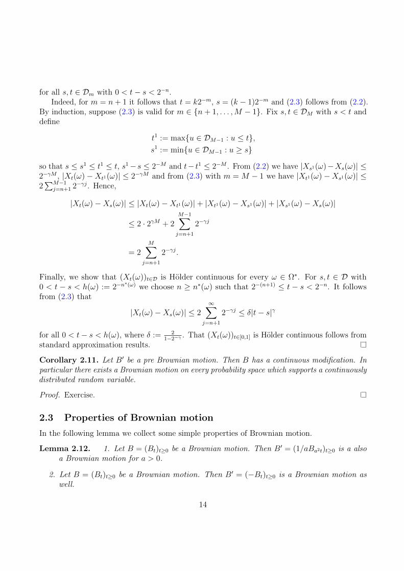
for all s, t ∈ Dm with 0 < t− s < 2−n.Indeed, for m = n+ 1 it follows that t = k2−m, s = (k − 1)2−m and (2.3) follows from (2.2).

By induction, suppose (2.3) is valid for m ∈ n+ 1, . . . ,M − 1. Fix s, t ∈ DM with s < t anddefine

t1 := maxu ∈ DM−1 : u ≤ t,s1 := minu ∈ DM−1 : u ≥ s

so that s ≤ s1 ≤ t1 ≤ t, s1−s ≤ 2−M and t− t1 ≤ 2−M . From (2.2) we have |Xs1(ω)−Xs(ω)| ≤2−γM , |Xt(ω)−Xt1(ω)| ≤ 2−γM and from (2.3) with m = M − 1 we have |Xt1(ω)−Xs1(ω)| ≤2∑M−1

j=n+1 2−γj. Hence,

|Xt(ω)−Xs(ω)| ≤ |Xt(ω)−Xt1(ω)|+ |Xt1(ω)−Xs1(ω)|+ |Xs1(ω)−Xs(ω)|

≤ 2 · 2γM + 2M−1∑j=n+1

2−γj

= 2M∑

j=n+1

2−γj.

Finally, we show that (Xt(ω))t∈D is Holder continuous for every ω ∈ Ω∗. For s, t ∈ D with0 < t − s < h(ω) := 2−n

∗(ω) we choose n ≥ n∗(ω) such that 2−(n+1) ≤ t − s < 2−n. It followsfrom (2.3) that

|Xt(ω)−Xs(ω)| ≤ 2∞∑

j=n+1

2−γj ≤ δ|t− s|γ

for all 0 < t− s < h(ω), where δ := 21−2−γ

. That (Xt(ω))t∈[0,1] is Holder continuous follows fromstandard approximation results.

Corollary 2.11. Let B′ be a pre Brownian motion. Then B has a continuous modification. Inparticular there exists a Brownian motion on every probability space which supports a continuouslydistributed random variable.

Proof. Exercise.

2.3 Properties of Brownian motion

In the following lemma we collect some simple properties of Brownian motion.

Lemma 2.12. 1. Let B = (Bt)t≥0 be a Brownian motion. Then B′ = (1/aBa2t)t≥0 is a alsoa Brownian motion for a > 0.

2. Let B = (Bt)t≥0 be a Brownian motion. Then B′ = (−Bt)t≥0 is a Brownian motion aswell.

14

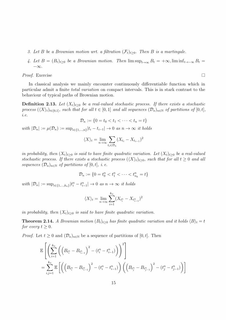
3. Let B be a Brownian motion wrt. a filtration (Ft)t≥0. Then B is a martingale.

4. Let B = (Bt)t≥0 be a Brownian motion. Then lim supt→∞Bt = +∞, lim inft→−∞Bt =−∞.

Proof. Exercise

In classical analysis we mainly encounter continuously differentiable function which inparticular admit a finite total variation on compact intervals. This is in stark contrast to thebehaviour of typical paths of Brownian motion.

Definition 2.13. Let (Xt)t≥0 be a real-valued stochastic process. If there exists a stochasticprocess (〈X〉t)t∈[0,1], such that for all t ∈ [0, 1] and all sequences (Dn)n∈N of partitions of [0, t],i.e.

Dn := 0 = t0 < t1 < · · · < tn = t

with |Dn| := µ(Dn) := supi∈1,...,n|ti − ti−1| → 0 as n→∞ it holds

〈X〉t = limn→∞

∑ti∈Dn

(Xti −Xti−1)2

in probability, then (Xt)t≥0 is said to have finite quadratic variation. Let (Xt)t≥0 be a real-valuedstochastic process. If there exists a stochastic process (〈X〉t)t≥0, such that for all t ≥ 0 and allsequences (Dn)n∈N of partitions of [0, t], i. e.

Dn := 0 = tn0 < tn1 < · · · < tnnk = t

with |Dn| := supi∈1,...,kn|tni − tni−1| → 0 as n→∞ it holds

〈X〉t = limn→∞

kn∑i=1

(Xtni−Xtni−1

)2

in probability, then (Xt)t≥0 is said to have finite quadratic variation.

Theorem 2.14. A Brownian motion (Bt)t≥0 has finite quadratic variation and it holds 〈B〉t = tfor every t ≥ 0.

Proof. Let t ≥ 0 and (Dn)n∈N be a sequence of partitions of [0, t]. Then

E

( kn∑i=1

((Btni−Btni−1

)2

− (tni − tni−1)

))2

=kn∑i,j=1

E[((

Btni−Btni−1

)2

− (tni − tni−1)

)((Btnj−Btnj−1

)2

− (tnj − tnj−1)

)]

15

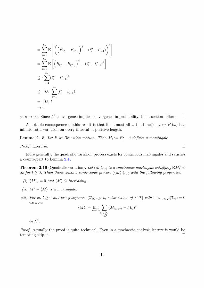
=kn∑i=1

E

[((Btni−Btni−1

)2

− (tni − tni−1)

)2]

=kn∑i=1

E[(Btni−Btni−1

)4

− (tni − tni−1)2

]

≤ ckn∑i=1

(tni − tni−1)2

≤ c|Dn|kn∑i=1

(tni − tni−1)

= c|Dn|t→ 0

as n→∞. Since L2-convergence implies convergence in probability, the assertion follows.

A notable consequence of this result is that for almost all ω the function t 7→ Bt(ω) hasinfinite total variation on every interval of positive length.

Lemma 2.15. Let B be Brownian motion. Then Mt := B2t − t defines a martingale.

Proof. Exercise.

More generally, the quadratic variation process exists for continuous martingales and satisfiesa counterpart to Lemma 2.15.

Theorem 2.16 (Quadratic variation). Let (Mt)t≥0 be a continuous martingale satisfying EM2t <

∞ for t ≥ 0. Then there exists a continuous process (〈M〉t)t≥0 with the following properties:

(i) 〈M〉0 = 0 and 〈M〉 is increasing.

(ii) M2 − 〈M〉 is a martingale.

(iii) For all t ≥ 0 and every sequence (Dn)n∈N of subdivisions of [0, T ] with limn→∞ µ(Dn) = 0we have

〈M〉t = limn→∞

∑ti∈Dnti≤t

(Mti+1∧t −Mti)2

in L2.

Proof. Actually the proof is quite technical. Even in a stochastic analysis lecture it would betempting skip it...

16

2.4 The Ito-integral

In this section we discuss the definition of a integrals of the form∫ T

0Ht dXt, where H and X

are stochastic processes. Such integrals are of fundamental importance not just for stochasticanalysis but also for mathematical finance. The reason is that they represent the continuoustime counterpart of the process (H ·X) encountered in the discrete time setup. We will comeback to this finance interpretation at a later stage.

As discussed in the previous section the paths of Brownian motion have infinite total variationon every finite interval. As a consequence we can not form a derivative dBt(ω)

dtand likewise it

does not work to define an stochastic integral in a ‘pathwise sense’: Given an arbitrary (saybounded continuous) stochastic process H there is not reason why the Riemann-Stiltjes integral(or the Lebesgue-Stiltjes integral) ∫ T

0

Ht(ω) dBt(ω) (2.4)

should exist. Indeed, for this we would need precisely that the function t 7→ Bt(ω) has finitetotal variation on the interval [0, T ].

The same problem occurs not only for Brownian motion but virtually for all (continuous)martingales which are not identically 0. A way out of this is to define integrals in slightlydifferent way. It turns out that a natural class of processes for which one can define a usefulstochastic integral consists in so called semi martingales :

Definition 2.17. A continuous adapted process X is a semimartingale1 if there exist a contin-uous martingale M and a continuous process A such that almost surely ω 7→ At(ω) has almostsurely finite variation on every finite interval with

X = M + A. (2.5)

Remark 2.18. 1. Apparently every martingale is a semi martingale and in particular Brow-nian motion is a semi martingale.

2. The semi-martingale decomposition in (2.5) is unique if we demand in addition thatA0 = 0.

3. The celebrated Doob-Meyer Theorem implies that every sub-martingale that is sufficientlybounded is a semi-martingale.

1Actually, this definition is not quite precise. Rigorously the following, wider definition should be used: Acontinuous process X is a semimartingale if it is locally the sum of a martingale and a finite variation process.I.e. if there exists a sequences of stopping times Tn, martingales Mn, and finite variation processes An such thatlimn T

n =∞ a.s. and Xt(ω) = Mnt (ω) + An

t (ω) for t ≤ Tn(ω).

17

Theorem 2.19. Assume that X is a semi-martingale and that H is a continuous boundedadapted process.

There exists a continuous adapted stochastic process I =: (H ·X) =:∫ .

0Hs dXs, such that

for all t ≥ 0 and all sequences (Dn)n∈N of partitions of [0, t], i.e.

Dn := 0 = tn0 < tn1 < · · · < tnnk = t

with |Dn| := supi∈1,...,kn|tni − tni−1| → 0 as n→∞ it holds

It = limn→∞

kn∑i=1

Htni(Xtni

−Xtni−1)

in probability.

Definition 2.20. In the context of Theorem 2.19, the process given by It = (H ·X)t =:∫ t

0Hs dXs

is called the Ito-integral or stochastic integral of H wrt. X.

It is straightforward to see that the Ito-integral is linear in both the integrand (H in theabove definition) as well as the integrator (X in the above definition).

Note also that if t 7→ At(ω) has almost surely finite variation and is continuous in t, then

the Ito-integral IT =∫ T

0Hs dAs satisfies

IT (ω) =

∫ T

0

Ht(ω) dAt(ω), (2.6)

where the right hand side of (2.6) denotes the usual Riemann-Stieltjes integral of the functiont 7→ Ht(ω) wrt. the continuous, finite variation function t 7→ At(ω).

Next we turn to the definition of stochastic integrals for so called simple integrands:

Definition 2.21. A process H = (Ht)t∈[0,T ] is called simple if

Ht(ω) =n∑i=1

H iI(si,si+1],

where 0 ≤ s1 ≤ . . . ≤ sn and each H i is Fsi-measurable and bounded. Let X be a continuousadapted process.

For simple integrands we set

(H ·X)u :=

∫ u

0

Hs dXs := Iu :=

∫ u

0

Ht dXt :=n∑i=1

H i(Xsi+1∧u −Xsi∧u).

18

The Ito-integral for simple integrands has a clear interpretation in mathematical financeterms: as in the discrete time setup, Xt stands for the price of a financial asset at time t,while Ht denotes the number of shares we hold at time t. Then (H · X)T represents exactlygains/losses accumulated from trading until time T .

The definition of the stochastic integral for simple processes connects to our previousdefinition through appropriate convergence results for stochastic integrals. Here we will onlymention a version of the dominated convergence Theorem of stochastic integration.

To state it, we need a definition.

Definition 2.22. A process L is called locally bounded if there exists a sequence of stoppingtimes τn, n ≥ 1, limn→∞ τn =∞ such that (t, ω) 7→ Lτnt (ω) := Lt∧τn(ω)(ω) is bounded for everyn.

Clearly every bounded process is locally bounded. We also have:

Lemma 2.23. Let L be a continuous process such that L0 is bounded. Then L is locally bounded.

Sketch of proof. The idea is to use that the sequence of stopping times given by

τn := inft ≥ 0 : |Lt| ≥ n.

Using this notion we can formulate a version of the dominated convergence Theorem forstochastic integrals:

Theorem 2.24. Let H,Hn, n ≥ 1 be adapted processes, which are simple or continuous. Assumethat L is a locally bounded process such that |H|, |Hn| ≤ L and that X is a continuous semimartingale. Then

limn→∞

(Hn ·X)T = (H ·X)T

in probability.

Proof. The proof of this result is beyond the scope of our lecture.

In view of Theorem 2.24 it is natural to try to extend the Ito-integral to all locally boundedintegrands that can be approximated by simple functions.

Definition 2.25. A process that is the pointwise limit of simple functions is called predictable.

Lemma 2.26. Every (left-)continuous adapted process is predictable.

Proof. Exercise.

If H is a predictable process which is locally bounded, the stochastic integral∫ T

0Hs dXs can

be defined by approximating with H with simple functions. Theorem 2.24 then applies also inthe case where H,Hn, n ≥ 1 are only predictable but not necessarily continuous or simple.

19

2.5 Alternative construction of the Ito-integral for Brownian motion

In this section we will sketch an alternative definition of the stochastic integral∫Ht dBt,

i.e. of the particular case where the integrator is Brownian motion. We fix T > 0 and concentrateon the interval [0, T ].

Definition 2.27.

(i) A function H : Ω× [0, T ]→ R is measurable, if it is F⊗B([0, T ])-measurable. It is adapted,if Ht(·) = H(·, t) is Ft-measurable for every t ∈ [0, T ].

(ii) Let

H2 := H2([0, T ])

:=

H : Ω× [0, T ]→ R measurable, adapted, E

[∫ T

0

H2s (·) ds

]<∞

.

(iii) Let

H20 :=

H =

n−1∑i=0

ai11(ti,ti+1] : 0 = t0 < t1 < · · · < tn = T, ai ∈ L2(Ω,Fti ,P),

for every i ∈ 0, . . . , n− 1, n ∈ N

.

(iv) For H =∑n−1

i=0 ai11(ti,ti+1] ∈ H20 let

(H ·B)T := I(H) :=

∫ T

0

H(·, s) dBs :=n−1∑i=0

ai(Bti+1−Bti).

Lemma 2.28 (Ito’s isometry). For H ∈ H20 we have

‖I(H)‖L2(Ω,F ,P) = ‖H‖L2(Ω×[0,T ],F⊗B([0,T ]),P⊗λ) .

Proof. Let H =∑n−1

i=0 ai11(ti,ti+1] ∈ H20. With Fubini’s theorem we obtain

‖H‖22 =

n−1∑i=0

E[a2i ](ti+1 − ti).

20

Moreover,

‖I(H)‖22 = E[I(H)2]

=n−1∑i,j=0

E[aiaj(Bti+1

−Bti)(Btj+1−Btj)

]=

n−1∑i=0

E[E[a2i (Bti+1

−Bti)2∣∣Fti]]

=n−1∑i=0

E[a2i ]E[(Bti+1

−Bti)2]

=n−1∑i=0

E[a2i ](ti+1 − ti),

where we have used the independence of the increments of B.

The following lemma is need to prove Proposition 2.30 below in which we obtain that the H20

is dense in H2 with respect to the L2-norm. Both the proof of the lemma and the propositionare quite technical. I put the proofs here for completeness but strongly suggest that you omitthem.

Lemma 2.29. Let H : Ω⊗ [0, T ]→ R be measurable and bounded. Then

limh↓0

E[∫ T

0

∣∣H(·, t)−H(·, (t− h)+)∣∣2 dt

]= 0.

Proof.

(i) For t ∈ [0, T ] and n ∈ N let

g(·, t) :=

∫ t

0

H(·, s) ds,

Hn(·, t) := n(g(·, t)− g

(·,(t− 1

n

)+))

so that |Hn(·, t)| ≤ n∫ t

(t− 1n

)+|H(·, s)| ds ≤ ‖H‖∞. Let

A :=

(ω, t) ∈ Ω× [0, T ] : limn→∞

Hn(ω, t) 6= H(ω, t),

Aω := t ∈ [0, T ] : (ω, t) ∈ A

for ω ∈ Ω. By the theorem of Lebesgue we have λ(Aω) = 0 for every ω ∈ Ω, henceP⊗ λ(A) = 0. Therefore, by dominated convergence

limn→∞

E[∫ T

0

|Hn(·, t)−H(·, t)|2 dt

]= 0.

21

(ii) For ε > 0 we can find n ∈ N and h0 > 0 such that

E[∫ T

0

|Hn(·, t)−H(·, t)|2 dt

]< ε

and

E[∫ T

0

∣∣Hn(·, (t− h)+)−H(·, (t− h)+∣∣2 dt

]≤ ε

for all 0 < h < h0. Using the triangle inequality we obtain

E[∫ T

0

∣∣H(·, t)−H(·, (t− h)+∣∣2 dt

] 12

≤ E[∫ T

0

|H(·, t)−Hn(·, t)|2 dt

] 12

+ E[∫ T

0

∣∣Hn(·, t)−Hn(·, (t− h)+)∣∣2 dt

] 12

+ E[∫ T

0

∣∣Hn(·, (t− h)+)−H(·, (t− h)+)∣∣2 dt

] 12

≤ 2ε+ E[∫ T

0

∣∣Hn(·, t)−Hn(·, (t− h)+)∣∣2 dt

] 12

.

We let h ↓ 0 and conclude from the continuity of t 7→ Hn(·, t) and the dominatedconvergence theorem that

limh↓0

E[∫ T

0

∣∣Hn(·, t)−Hn(·, (t− h)+)∣∣2 dt

] 12

= 0.

Proposition 2.30. The set H20 is dense in H2 with respect to the L2-norm.

Proof.

(i) Let H ∈ H2. For n ∈ N define Hn := (−n) ∨ (H ∧ n) which is bounded and adapted. Bydominated convergence ‖Hn −H‖2 → 0 as n→∞.

(ii) By (i) we can assume that H is measurable, bounded and adapted. We have to show thatthere exists (Hn)n∈N ⊆ H2

0 with ‖Hn −H‖2 → 0. To that end, for all n ∈ N and t ∈ Rdefine

ϕn(t) :=∑j∈Z

j − 1

2n11( j−1

2n, j2n ](t).

Since t− 12n≤ ϕn(t− s) + s < t and ϕn only takes discrete values, the process

Hn,s(·, t) := H(·, (s+ ϕn(t− s))+)

22

is adapted and a member of H20. Moreover, we claim that

E[∫ T

0

∫ 1

0

|Hn,s(·, t)−H(·, t)|2 ds dt

]→ 0 (2.7)

as n→∞. Indeed, for n ∈ N we have

E[∫ T

0

∫ 1

0

|Hn,s(·, t)− f(·, t)|2 ds dt

]= E

[∫ T

0

∫ 1

0

∣∣H (·, (s+ ϕn(t− s))+)−H(·, t)∣∣2 ds dt

]=∑j∈Z

E

[∫ T

0

∫[t− j

2n,t− j−1

2n )∩[0,1]

∣∣∣H (·, (s+ j−12n

)+)−H(·, t)

∣∣∣2 ds dt

]

≤ 2n(T + 1)E

[∫ T

0

∫ 2−n

0

∣∣H (·, (t− h)+)−H(·, t)

∣∣2 dh dt

]

= 2n(T + 1)

∫ 2−n

0

E[∫ T

0

∣∣H (·, (t− h)+)−H(·, t)

∣∣2 dt

]dh

→ 0

as n→∞ by Lemma 2.29. This shows (2.7).

Finally according to (2.7), there exists a subsequence (nk)k∈N such that (ω, t, s) 7→Hnk,s(ω, t) converges to f P ⊗ λ ⊗ λ-as. Fubini’s theorem implies Hnk,s → H P ⊗ λ-as for λ-almost all s ∈ [0, 1]. Hence, we may choose s ∈ [0, 1] such that Hnk,s → H P⊗λ-as.By dominated convergence we get

E[∫ T

0

|Hnk,s(·, t)−H(·, t)|2 dt

]→ 0

as k →∞. Since (Hnk,s)k∈N is a sequence in H20, the proof is complete.

Thus we can extend the stochastic integral from H20 to H2. Indeed, for H ∈ H2 let

(Hn)n∈N ⊆ H20 be a sequence such that ‖Hn −H‖2 → 0. In particular, (Hn)n∈N is a Cauchy

sequence in H2. By Lemma 2.28 we get

‖I(Hm)− I(Hn)‖2 = ‖I(Hm −Hn)‖2 = ‖Hm −Hn‖2

showing that (I(Hn))n∈N is a Cauchy sequence in L2(Ω,F ,P). Since L2(Ω,F ,P) is complete,we can define the stochastic integral

I(H) := limn→∞

I(Hn) ∈ L2(Ω,F ,P).

23

Remark 2.31. The stochastic integral I is well-defined. Suppose there exist two sequences(H1

n)n∈N and (H2n)n∈N converging to f ∈ L2 in L2. Then, by Lemma 2.28 we have∥∥I(H1

n)− I(H2n)∥∥

2=∥∥H1

n −H2n

∥∥2≤∥∥H1

n − f∥∥

2+∥∥H −H2

n

∥∥2→ 0

as n→∞.

Theorem 2.32 (Ito’s isometry). For H ∈ H2we have ‖H‖2 = ‖I(H)‖2.

Proof. Let (Hn)n∈N be a sequence in H20 such that ‖Hn −H‖2 → 0. By definition of I(H), we

have ‖I(Hn)− I(H)‖2 → 0, so that Lemma 2.28 yields

‖H‖2 = limn→∞

‖Hn‖2 = limn→∞

‖I(Hn)‖2 = ‖I(H)‖2 .

2.6 Ito’s formula

In this section we discuss the “chain rule of stochastic calculus”, the celebrated Ito-formula.For reference, let’s recall the usual chain rule:

(f g)′(t) = f ′(g)(t) · g′(t) ⇐⇒ df(g)

dt=df

dg

dg

dt= f ′(g)

dg

dt. (2.8)

Our goal is to derive a similar formula for the case where g is replaced by Brownian motion.As an intermediate step, we consider the case where g is not necessarily integrable but still

has finite variation. Formally we can multiply the right hand side of (2.8) with dt to obtain

df(g) = f ′(g)dg. (2.9)

To give (2.9) a rigorous meaning we need to write it in integrated form:

f(g(T ))− f(g(0)) =

∫ T

0

1 df(g) =

∫ T

0

f ′(g(t)) dg(t). (2.10)

The validity of (2.10) is a basic result for the Riemann-Stieltjes integral. We can ask ourselveswhether (2.10) remains true when we replace the finite variation function t 7→ g(t) with Brownianmotion t 7→ Bt. Remarkably, this is not the case, rather there is an additional correction term:

Theorem 2.33 (Ito’s formula). Let f ∈ C2(R).2 Then

f(Bt) = f(B0) +

∫ t

0

f ′(Bs) dBs +1

2

∫ t

0

f ′′(Bs) ds

for every t ∈ [0, T ].

2Let C2(R) denote the space of twice differentiable functions f : R→ R with continuous second derivative.

24

Usually Ito’s formula is given in a shorthand version similar to (2.9). It then reads

df(Bt) = f ′(Bt) dBt +1

2f ′′(Bt)dt. (2.11)

We will first give a heuristic derivation of (2.11). The key idea is that, informally, Theorem 2.14on the quadratic variation of Brownian motion asserts that

dB2t = dt (2.12)

. To estimate df(Bt) we can then use Taylor’s formula to obtain

df(Bt) = f(Bt+dt)− f(Bt) = f((Bt) + dBt)− f(Bt) (2.13)

= f ′(Bt)dBt +1

2f ′′(Bt)dB

2t +

1

6f ′′′(Bt)dB

3t + . . . (2.14)

= f ′(Bt)dBt +1

2f ′′(Bt)dB

2t . (2.15)

Note that all terms including dBnt , n ≥ 3 are of higher order than dt an thus do not contribute to

sum. However the term dB2t is of the same order as dt (in fact equal to it) and thus leads to an

important contribution. This is the decisive difference to the case of finite variation functions.In the remainder of this section, we give a rigorous proof of Ito’s formula. I think that it

doesn’t add that much to the heuristic discussion above, feel free to skip it. The proof of Ito’sformula is based on the following result.

Theorem 2.34. Let f : R→ R be continuous, ti := inT for i ∈ 0, . . . , n. Then

n∑i=1

f(Bti−1)(Bti −Bti−1

)→∫ T

0

f(Bs) dBs

in probability as n→∞.

Proof.

(i) For m ∈ N letτm := inft ≥ 0 : |Bt| ≥ m ∧ T.

Then (τm)m∈N is a localizing sequence for f(B). Further, there exists a continuous functionfm : R→ R with compact support and f |[−m,m] = fm|[−m,m]. By construction∫ ·

0

f(Bs) dBs =

∫ ·0

fm(Bs) dBs

on [0, τm].

25

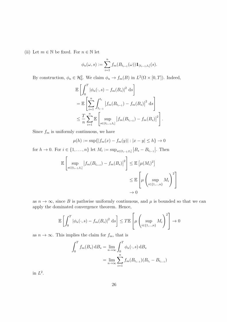
(ii) Let m ∈ N be fixed. For n ∈ N let

φn(ω, s) :=n∑i=1

fm(Bti−1(ω))11(ti−1,ti](s).

By construction, φn ∈ H20. We claim φn → fm(B) in L2(Ω× [0, T ]). Indeed,

E[∫ T

0

|φn(·, s)− fm(Bs)|2 ds

]= E

[n∑i=1

∫ ti

ti−1

∣∣fm(Bti−1)− fm(Bs)

∣∣2 ds

]

≤ T

n

n∑i=1

E

[sup

s∈(ti−1,ti]

∣∣fm(Bti−1)− fm(Bs)

∣∣2] .Since fm is uniformly continuous, we have

µ(h) := sup|fm(x)− fm(y)| : |x− y| ≤ h → 0

for h→ 0. For i ∈ 1, . . . , n let Mi := sups∈(ti−1,ti]

∣∣Bs −Bti−1

∣∣. Then

E

[sup

s∈(ti−1,ti]

∣∣fm(Bti−t)− fm(Bs)∣∣2] ≤ E

[µ(Mi)

2]

≤ E

µ( supi∈1,...,n

Mi

)2

→ 0

as n → ∞, since B is pathwise uniformly continuous, and µ is bounded so that we canapply the dominated convergence theorem. Hence,

E[∫ T

0

|φn(·, s)− fm(Bs)|2 ds

]≤ TE

µ( supi∈1,...,n

Mi

)2→ 0

as n→∞. This implies the claim for fm, that is∫ T

0

fm(Bs) dBs = limn→∞

∫ T

0

φn(·, s) dBs

= limn→∞

n∑i=1

fm(Bti−1)(Bti −Bti−1

)

in L2.

26

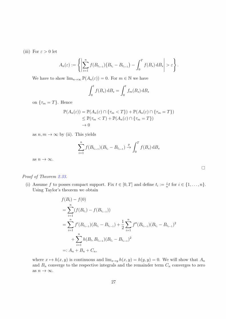
(iii) For ε > 0 let

An(ε) :=

∣∣∣∣∣n∑i=1

f(Bti−1)(Bti −Bti−1

)−∫ T

0

f(Bs) dBs

∣∣∣∣∣ > ε

.

We have to show limn→∞ P(An(ε)) = 0. For m ∈ N we have∫ t

0

f(Bs) dBs =

∫ t

0

fm(Bs) dBs

on τm = T. Hence

P(An(ε)) = P(An(ε) ∩ τm < T) + P(An(ε) ∩ τm = T)≤ P(τm < T ) + P(An(ε) ∩ τm = T)→ 0

as n,m→∞ by (ii). This yields

n∑i=1

f(Bti−1)(Bti −Bti−1

)P→∫ T

0

f(Bs) dBs

as n→∞.

Proof of Theorem 2.33.

(i) Assume f to posses compact support. Fix t ∈ [0, T ] and define ti := int for i ∈ 1, . . . , n.

Using Taylor’s theorem we obtain

f(Bt)− f(0)

=n∑i=1

(f(Bti)− f(Bti−1))

=n∑i=1

f ′(Bti−1)(Bti −Bti−1

) +1

2

n∑i=1

f ′′(Bti−1)(Bti −Bti−1

)2

+n∑i=1

h(Bt, Bti−1)(Bti −Bti−1

)2

=: An +Bn + Cn,

where x 7→ h(x, y) is continuous and limx→y h(x, y) = h(y, y) = 0. We will show that Anand Bn converge to the respective integrals and the remainder term Cn converges to zeroas n→∞.

27

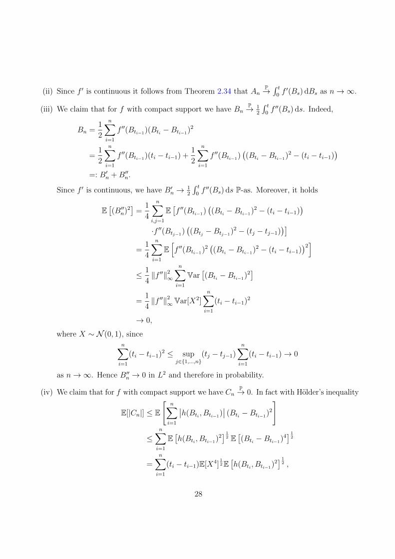
(ii) Since f ′ is continuous it follows from Theorem 2.34 that AnP→∫ t

0f ′(Bs) dBs as n→∞.

(iii) We claim that for f with compact support we have BnP→ 1

2

∫ t0f ′′(Bs) ds. Indeed,

Bn =1

2

n∑i=1

f ′′(Bti−1)(Bti −Bti−1

)2

=1

2

n∑i=1

f ′′(Bti−1)(ti − ti−1) +

1

2

n∑i=1

f ′′(Bti−1)((Bti −Bti−1

)2 − (ti − ti−1))

=: B′n +B′′n.

Since f ′ is continuous, we have B′n → 12

∫ t0f ′′(Bs) ds P-as. Moreover, it holds

E[(B′′n)2

]=

1

4

n∑i,j=1

E[f ′′(Bti−1

)((Bti −Bti−1

)2 − (ti − ti−1))

·f ′′(Btj−1)((Btj −Btj−1

)2 − (tj − tj−1))]

=1

4

n∑i=1

E[f ′′(Bti−1

)2((Bti −Bti−1

)2 − (ti − ti−1))2]

≤ 1

4‖f ′′‖2

∞

n∑i=1

Var[(Bti −Bti−1

)2]

=1

4‖f ′′‖2

∞Var[X2]n∑i=1

(ti − ti−1)2

→ 0,

where X ∼ N (0, 1), sincen∑i=1

(ti − ti−1)2 ≤ supj∈1,...,n

(tj − tj−1)n∑i=1

(ti − ti−1)→ 0

as n→∞. Hence B′′n → 0 in L2 and therefore in probability.

(iv) We claim that for f with compact support we have CnP→ 0. In fact with Holder’s inequality

E[|Cn|] ≤ E

[n∑i=1

∣∣h(Bti , Bti−1)∣∣ (Bti −Bti−1

)2

]

≤n∑i=1

E[h(Bti , Bti−1

)2] 1

2 E[(Bti −Bti−1

)4] 1

2

=n∑i=1

(ti − ti−1)E[X4]12E[h(Bti , Bti−1

)2] 1

2 ,

28

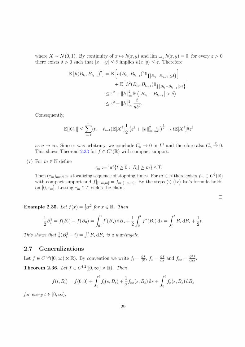
where X ∼ N (0, 1). By continuity of x 7→ h(x, y) and limx→y h(x, y) = 0, for every ε > 0there exists δ > 0 such that |x− y| ≤ δ implies h(x, y) ≤ ε. Therefore

E[h(Bti , Bti−1

)2]

= E[h(Bti , Bti−1

)211|Bti−Bti−1|≤δ]

+ E[h2(Bti , Bti−1

)11|Bti−Bti−1|>δ]

≤ ε2 + ‖h‖2∞ P

(∣∣Bti −Bti−1

∣∣ > δ)

≤ ε2 + ‖h‖2∞

t

nδ2.

Consequently,

E[|Cn|] ≤n∑i=1

(ti − ti−1)E[X4]1

2

(ε2 + ‖h‖2

∞tnδ2

) 12 → tE[X4]

12 ε2

as n→∞. Since ε was arbitrary, we conclude Cn → 0 in L1 and therefore also CnP→ 0.

This shows Theorem 2.33 for f ∈ C2(R) with compact support.

(v) For m ∈ N defineτm := inft ≥ 0 : |Bt| ≥ m ∧ T.

Then (τm)m∈N is a localizing sequence of stopping times. For m ∈ N there exists fm ∈ C2(R)with compact support and f |[−m,m] = fm|[−m,m]. By the steps (i)-(iv) Ito’s formula holdson [0, τm]. Letting τm ↑ T yields the claim.

Example 2.35. Let f(x) = 12x2 for x ∈ R. Then

1

2B2t = f(Bt)− f(B0) =

∫ t

0

f ′(Bs) dBs +1

2

∫ t

0

f ′′(Bs) ds =

∫ t

0

Bs dBs +1

2t.

This shows that 12(B2

t − t) =∫ t

0Bs dBs is a martingale.

2.7 Generalizations

Let f ∈ C1,2([0,∞)× R). By convention we write ft = ∂f∂t

, fx = ∂f∂x

and fxx = ∂2f∂xx

.

Theorem 2.36. Let f ∈ C1,2([0,∞)× R). Then

f(t, Bt) = f(0, 0) +

∫ t

0

ft(s, Bs) +1

2fxx(s, Bs) ds+

∫ t

0

fx(s, Bs) dBs

for every t ∈ [0,∞).

29

In short we would express this as

df(t, Bt) =

[ft(t, Bt) +

1

2fxx(t, Bt)

]dt+ fx(t, Bt) dBt. (2.16)

As above, it is not hard to argue this on an intuitive level using Taylor’s formula. We have:

df(t, Bt) = f(t+ dt, Bt+dt)− f(Bt) =

= ft(t, Bt)dt+ fxx(t, Bt)dBt +1

2fxx(t, Bt)dB

2t + ftx(t, Bt)dtdBt +

1

6ftxx(t, Bt)dB

2t + . . .

= ft(t, Bt)dt+ fx(t, Bt)dBt +1

2fxx(t, Bt)dB

2t .

As before we use here that all terms of order dtdBt, dB3t and higher do not contribute at the

level of dt. We thus obtain (2.16) based on dB2t = dt.

We do not discuss a rigorous version of this argument which in any case would be verysimilar to the one in the previous section.

The Ito-formula in (2.16) is again just a very special case of a much more general Ito formulafor semimartingales.

To state this general version of the Ito-formula we need the concept of quadratic co-variation:

Definition 2.37. Let (Xt)t≥0, (Yt)t≥0 be a real-valued stochastic processes. A stochastic process(〈X, Y 〉t)t∈[0,1], such that for all t ∈ [0, 1] and all sequences (Dn)n∈N of partitions of [0, t] with|Dn| := µ(Dn) := supi∈1,...,n|ti − ti−1| → 0 as n→∞ it holds

〈X, Y 〉t = limn→∞

∑ti∈Dn

(Xti −Xti−1)(Yti − Yti−1

)

in probability, is called the quadratic co-variation process of X, Y .

If X, Y are continuous semi-martingales, 〈X, Y 〉 exists. Apparently we have 〈X,X〉 = 〈X〉.It is also easy to see that

〈X, Y 〉 =1

4(〈X + Y 〉 − 〈X − Y 〉). (2.17)

Often the quadratic covariation process is defined simply through (2.17). (A definition of thistype is called ‘definition by polarization’.)

Using this concept we have the following version of Ito’s formula: Assume that f : R2 → Ris C2 and that X, Y are continuous semi-martingales. Then we have

df(Xt, Yt) = fx(Xt, Yt)dXt + fy(Xt, Yt)dYt+

1/2fxx(Xt, Yt)d〈X〉t + fxy(Xt, Yt)d〈X, Y 〉t + 1/2fyy(Xt, Yt)d〈Y 〉t.(2.18)

Naturally, an analogue of (2.18) for functions in more than two variables is valid as well. Weomit it due to the more complicated notations. Likewise we omit the integral form of (2.18)and its proof.

In the next section we will describe a class of semi-martingales for which we can calculatethe quadratic covariation process explicitly.

30

2.8 Ito-processes

Let (Ω,F ,P) be a probability space, B = (Bt)t∈[0,T ] a Brownian motion with standard filtration(Ft)t∈[0,T ].

Definition 2.38. A continuous stochastic process X = (Xt)t∈[0,T ] is called Ito process, if

Xt = X0 +

∫ t

0

a(·, s) ds+

∫ t

0

b(·, s) dBs,

where X0 ∈ R, a, b : Ω × [0, T ] → R are F ⊗ B([0, T ])-measurable and adapted such that∫ T0|a(·, s)| ds <∞ and

∫ T0|b(·, s)|2 ds <∞ P-as.

Ito-processes are a relatively tractable class of stochastic processes that is sufficiently generalto cover many important applications. In this section we collect basic results concerning Ito-processes as integrators and the quadratic variation of Ito-processes. We will omit the respectiveproofs but emphasize that they usually follow a rather basic scheme: First one proves the resultsfor the case where the ‘coefficients’ a, b are simple processes which is fairly straightforward.Then one establishes the general case through limiting arguments.

Proposition 2.39. Let Xt = X0 +∫ t

0a(·, s) ds+

∫ t0b(·, s) dBs be an Ito process. Then for f : Ω×

[0, T ]→ R measurable and adapted with∫ T

0|f(·, s)a(·, s)| ds <∞ and

∫ T0|f(·, s)b(·, s)|2 ds <∞

P-as the Ito integral is given by∫ t

0

f(·, s) dXs =

∫ t

0

f(·, s)a(·, s) ds+

∫ t

0

f(·, s)b(·, s) dBs.

Proposition 2.40. Let X be an Ito process with representation

X = X10 +

∫ ·0

a1(·, s) ds+

∫ ·0

b1(·, s) dBs

= X20 +

∫ ·0

a2(·, s) ds+

∫ ·0

b2(·, s) dBs.

Then X10 = X2

0 , a1 = a2 and b1 = b2 P⊗ λ-as.

Theorem 2.41 (Quadratic variation of an Ito process). Let

X =

∫ ·0

a(·, s) ds+

∫ ·0

b(·, s) dBs

be an Ito process. Then

〈X〉t =

∫ t

0

b2(·, s) ds.

31

Let

X i =

∫ ·0

ai(·, s) ds+

∫ ·0

bi(·, s) dBs, i = 1, 2

be Ito processes. Then

〈X1, X2〉t =

∫ t

0

b1(·, s)b2(·, s) ds.

Informally we would express this result as

d〈X1, X2〉 = b1t b

2t dt (2.19)

We conclude this section by giving the Ito-formula for Ito-processes. Importantly this is justa special case of (2.18) (in particular it is recommended to only memorize (2.18) and the ‘rule’given in (2.19)).

Theorem 2.42. Let f ∈ C1,2([0,∞)×R) and X =∫ ·

0a(·, s) ds+

∫ ·0b(·, s) dBs be an Ito process.

Then we have

f(t,Xt) = f(0, 0) +

∫ t

0

ft(s,Xs) ds+

∫ t

0

fx(s,Xs) dXs +1

2

∫ t

0

fxx(s,Xs) d〈X〉s

= f(0, 0) +

∫ t

0

(ft(s,Xs) + fx(s,Xs)a(·, s) +

1

2fxx(s,Xs)b

2(·, s))

ds

+

∫ t

0

fx(s,Xs)b(·, s) dBs

for every t ∈ [0, T ].

2.9 Introduction to stochastic differential equations

We consider stochastic differential equations (SDE) of the formdXt = µ(t,Xt) dt+ σ(t,Xt) dBt,

X0 = x0,

where x0 ∈ R. This equation should be interpreted as an informal way of expressing thecorresponding integral equation

Xt = x0 +

∫ t

0

µ(s,Xs) ds+

∫ t

0

σ(s,Xs) dBs.

In view of our goals later on, the following example is the most important part of this section:

32

Example 2.43 (Geometric Brownian motion). We consider the SDEdXt = µXt dt+ σXt dBt,

X0 = x0,

where x0, µ ∈ R and σ > 0. We start by making the ansatz Xt = f(t, Bt). By Ito’s formula weobtain

dXt = ft(t, Bt) dt+ fx(t, Bt) dBt + 12fxx(t, Bt) dt

=(ft(t, Bt) + 1

2fxx(t, Bt)

)dt+ fx(t, Bt) dBt

!= µXt dt+ σXt dBt

= µf(t, Bt) dt+ σf(t, Bt) dBt.

By comparison of coefficients we get µf = ft + 12fxx and σf = fx. From the second equation we

obtainf(t, x) = exp(σx+ g(t))

for (t, x) ∈ [0,∞)× R. Plugging in f into the first equation yields

µf = g′f + 12σ2f,

so that for instanceg(t) =

(µ− 1

2σ2)t

for t ∈ [0,∞). Hence,Xt = x0 exp

(σBt +

(µ− 1

2σ2)t)

which is the Black-Scholes model, the price process of a financial asset with drift µ and volatilityσ.

For completeness we state (without proof) the most important criterion for existence anduniqueness of solutions to SDEs. The Lipschitz conditions appearing therein should be familiarfrom the theory of deterministic ODEs.

Theorem 2.44 (Existence and uniqueness of solutions). Let µ, σ : [0,∞)× R→ R such that

|µ(t, x)− µ(t, y)|2 + |σ(t, x)− σ(t, y)|2 ≤ K|x− y|2,|µ(t, x)|2 + |σ(t, x)|2 ≤ K

(1 + |x|2

)hold for all t ∈ [0, T ], x, y ∈ R for some K > 0. Then the SDE

dXt = µ(t,Xt) dt+ σ(t,Xt) dBt,

X0 = x0,

has a unique continuous, adapted solution with supt∈[0,T ] E [|Xt|2] <∞.

33

2.10 Stochastic integral and martingales

Recall that a process H = (Ht)t∈[0,T ] is simple if

Ht(ω) =n∑i=1

H iI(si,si+1],

where 0 ≤ s1 ≤ . . . ≤ sn and each H i is Fsi-measurable and that for simple integrands thestochastic integral is given by

(H ·X)u :=

∫ u

0

Hs dXs := Iu :=

∫ u

0

Ht dXt :=n∑i=1

H i(Xsi+1∧u −Xsi∧u). (2.20)

From this definition it is straight forward (Exercise) to see that if M is a continuous martingaleand H is a bounded simple process, then (H ·M)t, t ∈ [0, T ] is a continuous martingale.

Using limiting arguments, this can be extended to the case of general H. For instance onecan prove:

Proposition 2.45. Let H be a bounded predictable process and let M be a continuous martingale.Then (H ·M)t, t ∈ [0, T ] is a continuous martingale.

(More generally, if H is locally bounded and M is a continuous martingale, then (H ·M) iscontinuous local martingale.)

As usual, such results are simpler to prove in the case where we are integrating againstBrownian motion. In this case we have the following:

Theorem 2.46. Let B be a Brownian motion and ϕ ∈ H2([0, T ]). Then

Xt :=

∫ t

0

ϕs dBs

is a continuous martingale and E[X2T ] <∞.

Proof. Exercise.

We also note that an Ito-process is a martingale only if the “dt-part” vanishes: the Itoprocess

Xt = X0 +

∫ t

0

a(·, s) ds+

∫ t

0

b(·, s) dBs,

is a martingale if and only if a(·, ·) = 0, P ⊗ λ-a.s. (Exercise.) In view of this, the term∫ t0a(·, s) ds is called drift part, while

∫ t0b(·, s) dBs is called martingale part.

The above comments should are probably not very surprising. In contrast the followingrepresents a rather remarkable converse of Theorem 2.46:

34

Theorem 2.47 (martingale representation theorem). Let (Bt)Tt=0 be Brownian motion and

write F = (Ft)t∈[0,T ] for the filtration generated by B. Let (Xt)t∈[0,T ] be a martingale adapted to(Ft)t∈[0,T ] and E[X2

T ] <∞. Then there exists a unique ϕ ∈ H2([0, T ]) such that

Xt = X0 +

∫ t

0

ϕs dBs (2.21)

for every t ∈ [0, T ].

Below we will prove an important special case of Theorem 2.47. Before going into this,we make some important comments: First of all X0 = EXT since F0 is the trivial σ-algebra.Moreover, uniqueness of φ is a straight forward consequence of Ito’s isometry.

Next we claim that it is sufficient for Theorem 2.47 to show that for each X ∈ L2(Ω,FT ,P)there exists ϕ ∈ H2([0, T ]) such that

XT = E[X0] +

∫ T

0

ϕt dBt. (2.22)

Indeed, (2.21) follows from (2.22) by applying the conditional expectation operator E[·|Ft].We will now prove (2.22) in an important and instructive case:Assume that X = f(BT ), where f ∈ C2(R) is such that E[f(BT )2] < ∞. We define the

martingale (Xt)t∈[0,T ] through Xt = E[f(BT )|Ft]. The crucial point is to notice that there existsa function f(t, b), (t, b) ∈ [0, T ]× R such that

E[f(BT )|Ft] = f(t, Bt). (2.23)

To see this, note first that E[f(BT )|Ft] = E[f(Bt + (BT −Bt))|Ft] = E[f(Bt + (BT −Bt))|Bt]since (BT −Bt) is independent of Ft. Moreover E[f(Bt + (BT −Bt))|Bt] = f(t, Bt), where

f(t, b) :=

∫f(b+ y) dγT−t(y) (2.24)

and γT−t denotes the centered Gaussian with variance T − t. (Exercise.)Since f ∈ C2, we can apply Ito’s formula to the process Xt = f(t, Bt) to obtain

dXt = fx(t, Bt) dBt + [fxx(t, Bt) + ft(t, Bt)] dt. (2.25)

Next we note that the drift term [fxx(t, Bt) + ft(t, Bt)] vanishes. This can either be showndirectly from the definition of f(t, b) or, more elegantly, by noticing that the drift term vanishesnecessarily since Xt = E[f(BT )|Ft] is a martingale by definition. It follows that (3.12) asserts(in integral form) that

Xt = X0 +

∫ t

0

fx(u,Bu) dBu (2.26)

35

as required.Summing up, in the particular case where XT is given in the form f(BT ) we have not

only established the martingale representation theorem, but we have also found an explicitrepresentation of the required integrand ϕ.

We note that the approach presented here can in fact be used to establish Theorem 2.47 in thegeneral case: In the first step, one iterates the above idea to provide an explicit representationin the case where X = f(Bt1 , . . . , Btn) for 0 ≤ t1 ≤ . . . ≤ tn ≤ T . Then, in the second step, oneuses that the set of all X of this form is dense in L2(Ω,FT ,P).

We close this section with a result two results that will not be required in the remainderof this lecture but are very much connected to the above ideas on representing martingales interms of Brownian motion. Moreover they highlight the particular role the Brownian motionhas in stochastic analysis.

Theorem 2.48 (Levy’s characterization of Brownian motion). Let M be a continuous (local)martingale starting at M0 = 0 and assume that 〈M〉t = t for t ≥ 0. Then M is Brownianmotion.

Sketch of proof. What we should prove that differences of the form Mti+1−Mti are Gaussian

with variance ti+1 − ti. Instead of this we just show that Mt ∼ N(0, t). (The general case wouldfollow using the same idea.) To do this we will calculate the moment generating function

λ 7→ E exp (λMt) = φt(λ).

To show that Mt ∼ N(0, t) we need to prove that φt is the moment generating function of theappropriate normal distribution, i.e. that φt(λ) = 1

2λ2t. To do this we consider the process

Xt := exp (λMt − 12λ2t).

By Ito’s formula, we have

dXt = λXt dMt + 12λ2d〈Mt〉 − 1

2λ2 dt = λXt dMt.

Ignoring issues of boundedness, we thus obtain that X is a martingale hence we have

E exp (λMt − 12λ2t) = EXt = EX0 = 1

which yields E exp (λMt) = 12λ2t as required.

In order to give the real proof, one usually works with the characteristic functions instead ofthe moment generating function since this avoids (as usual) problems associated to boundedness.I went with the moment generating function to avoid considering complex numbers.

Let X be a stochastic process, let (τt)t≥0 be a family of stopping times such that for s < twe have τs ≤ τt. Then Yt := Xτt , t ≥ 0 is called a time-change of X.

In essence, the following results says that every continuous martingale looks like Brownianmotion up to a time-change.

36

Corollary 2.49. Let M be a continuous martingale such that M0 = 0 and 〈M〉∞ =∞. Set

τt := infu ≥ 0 : 〈M〉u = t.

Then Bt := Mτt is a Brownian motion.

Sketch of Proof. To establish this, one proves that a time-change of a martingale is still amartingale and that

〈B〉t = 〈M〉τt = t.

Then Levy’s characterization theorem applies.

2.11 Girsanov’s Theorem

In this section we present the final ingredient from stochastic analysis that is important for ourconsiderations in mathematical finance.

A basic viewpoint on this result is the following: Consider a Brownian motion with drift, say

Xt := Bt + µ · t, t ≥ 0,

where µ is a positive constant. We are interested to determine in which sense X behaves isdifferent from a Brownian motion.

First of all note that the paths of X still have the same quadratic variation as the paths ofB since the finite variation part is irrelevant for this.

A crucial difference between X and B is the following: At time t the paths of B are (onaverage) close to 0, paths which are at level ±µt are relatively rare. In contrast, typical pathsof X at time t are at height µt, while paths which are at level 0 (or 2µt) are rare. The ideabehind Girsanov’s theorem is that one can turn X into a Brownian motion by changing theprobability of individual paths: I.e., to make X look like a Brownian motion, paths which endat 0 should get a much higher weight while paths that end at µt should get a much smallerweight. In Girsanov’s Theorem one changes the underlying measure accordingly, so that Xbecomes a Brownian motion.

Theorem 2.50 (Girsanov). For T > 0 let µ ∈ H2([0, T ]) be bounded. Consider

Xt := Bt +

∫ t

0

µs ds

and

Mt := exp

(−∫ t

0

µs dBs −1

2

∫ t

0

µ2s ds

)for t ∈ [0, T ]. Define Q by dQ

dP := MT .

(i) The process (Mt)t∈[0,T ] is a P-martingale.

37

(ii) The process (XtMt)t∈[0,T ] is a P-martingale.

(iii) The process (Xt)t∈[0,T ] is a Q-Brownian motion.

(As common by now, I advise to only skim over the proof.)

Proof.

(i) Ito’s formula applied to the Ito process

Ft := −∫ t

0

µs dBs −1

2

∫ t

0

µ2s ds

yields

dMt = exp(Ft) dFt + 12

exp(Ft) d〈F 〉t= −Mtµt dBt − 1

2Mtµ

2t dt+ 1

2Mtµ

2t dt

= −µtMt dBt.

Hence, M is a positive local martingale and therefore a supermartingale (by Fatou’slemma). Moreover, for t ∈ [0, T ] and every p > 1 we have

Mpt = exp

(−∫ t

0

pµs dBs −1

2

∫ t

0

(pµs)2 ds

)exp

(p(p− 1)

2

∫ t

0

µ2s ds

)= St exp

(p(p− 1)

2

∫ t

0

µ2s ds

),

where S is a supermartingale. Therefore, with |µ| ≤ c we obtain

E[∫ T

0

µ2sM

2s ds

]≤ c2

∫ T

0

E[M2s ] ds ≤ c2T exp(c2T ).

Hence, µM ∈ H2([0, T ]) so that M is a P-martingale. In particular, we have E[MT ] =M0 = 1.

(ii) Let Y := XM . It holds

dXt = dBt + µt dt,

dMt = −µtMt dBt

so that d〈X,M〉t = −µtMt dt. By the product formula we get

dYt = Xt dMt +Mt dXt + d〈X,M〉t= −µtMtXt dBt +Mt dBt +Mtµt dt− µtMt dt

= Mt(1− µtXt) dBt.

38

Therefore Y is a local martingale. Moreover, using Holder’s inequality and (i) we have

E[∫ T

0

M2s (1− µsXs)

2 ds

]≤ E

[∫ T

0

M2s (1 + µ2

s +X2s + µ2

sX2s ) ds

]≤ (1 + c2)

(E[∫ T

0

M2s ds

]+ E

[∫ T

0

M4s ds

] 12

E[∫ T

0

X4s ds

] 12

)<∞.

Hence, M(1− µX) ∈ H2([0, T ]) so that Y is a P-martingale.

(iii) Let 0 ≤ s ≤ t ≤ T and A ∈ Fs. Then

EQ[Xt11A] = E[MTXt11A]

= E[MtXt11A]

= E[MsXs11A]

= E[MTXs11A]

= EQ[Xs11A].

Hence X is a Q-martingale. By Levy’s characterization Theorem, X is a Q-Brownianmotion.

3 The financial models of Bachelier and Black-Scholes

3.1 The Bachelier model

Louis Bachelier (1870-1946). We assume that the asset follows the dynamics

Xt = x0 +mt+ σBt,

where m ∈ R is the drift parameter, σ > 0 is called the volatility and (Bt)t∈[0,∞) is a Brownianmotion on (Ω,F ,P) with standard Brownian filtration (Ft)t∈[0,∞). It is our goal to find areplicating strategy for a contingent claim of the form f(XT ), where f : R→ [0,∞). As usualwe are particularly interested in European Call / Put options.

Example 3.1.

(i) Let f : R→ [0,∞), x 7→ (x−K)+, then (XT −K)+ is a European call option with strikeprice K > 0.

39

(ii) Let f : R→ [0,∞), x 7→ (K − x)+, then (K −XT )+ is a European put option with strikeprice K > 0.

According to Girsanov’s theorem,

B∗t := Bt +m

σt

defines a P∗-Brownian motion, where dP∗

dP = exp(−mσBT − m2

2σ2T ). In particular,

Xt = x0 + σB∗t

is a P∗-martingale, that is P∗ is an equivalent martingale measure.The principle idea is now to apply the martingale representation theorem to the P∗-martingale

Mt := EP∗ [f(XT )|Ft]. Since our payoff function has a very simple form, we will even obtainexplicit formulas:

Define g(b∗) := f(x0 + σb∗) and

g(t, b∗) := EP∗ [g(B∗)|Ft]

so that g(t, B∗t ) = Mt. As in (3.11) we have

g(t, b) =

∫g(b+ y) dγT−t(y) (3.1)

and

Mt = M0 +

∫ t

0

gb(s, B∗s )dB

∗s . (3.2)

In terms of X we can rewrite this as

Mt = M0 +

∫ t

0

1σgb(s, (Xs − x0)/σ)dX∗s .

Noting that M0 = EP∗ [f(XT )] =: p we thus obtain

f(XT ) = p+ (H ·X)T , (3.3)

where Ht = 1σgb(t, (Xt − x0)/σ).

Remark 3.2. In the above treatise we have been imprecise at two points:

1. To arrive at (3.11), we would like the function f(t, x), or, g(t, b), resp. to be C2. This isnot the case if take f to be a European put / call function. However this can be easilyovercome: The convolution with respect to a Gaussian in (3.1) is ‘smoothing’ and henceg(t, b) is C2 for t < T . It is then not hard to see that this is enough for our arguments togo through.

40

2. We would like the hedging relation (3.3) to hold with respect to P but our derivation waswith respect to the measure P∗. In principle there could be problem here since the stochasticintegral was defined with a fixed underlying probability measure in mind. However, thisis not an issue since the stochastic integral remains the same as long as one switches toan equivalent probability. This is trivial as long as one considers only simple integrands.Moreover this remains true when passing to limits in probability (which remains unalteredunder changes to an equivalent probability measure) which allows us to conclude.

Example 3.3. Consider again the European call option f(XT ) = (XT − K)+. Since f isincreasing and 1-Lipschitz, it follows that g is increasing and σ-Lipschitz. Since these propertiesare preserved under convolution with a Gaussian, g(t, .) is also increasing and σ-Lipschitz.As the convolution operator smoothes, g(t, .) is differentiable for t ∈ [0, T ) and the derivativesatisfies gb(t, .) ∈ [0, σ]. Considering the hedging strategy obtained in (3.2), we find that

Ht(Xt) = 1σgb(t, (Xt − x0)/σ) ∈ [0, 1].

In particular, it is no “short-selling” is necessary to hedge a European call option in theBachelier-model.

Note also that convexity of f implies that gb(t, ·) and then also Ht(·) is increasing.

Theorem 3.4. In the Bachelier model, the fair price of a contingent claim f(XT ) is given byEP∗ [f(XT )].

More generally then Theorem 3.4 we have:

Theorem 3.5. Let G ∈ L2(Ω,FT ,P∗) be a contingent claim. Then there exists a unique pair(a,H), a ∈ R, H ∈ H2(0, T ) such that

a+ (H ·X)T = G. (3.4)

Moreover we have a = EP∗ [G].

Proof. We apply the martingale representation theorem to G and the P∗-Brownian motion B∗

to obtain a strategy H such that

EP∗ [G] +

∫ T

0

H dB∗ = G.

Setting Ht := 1σHt for t ≤ T we arrive at

G = EP∗ [G] +

∫ T

0

H d(σB∗) = EP∗ [G] +

∫ T

0

H dX.

As in the martingale representation theorem, a and H are uniquely determined.

41

In reminiscence of Theorem 1.24 a consequence of Theorem 3.14 is the following:

Theorem 3.6. The measure P∗ is the only equivalent martingale measure.

Idea of proof. For instance one can show that the claims of the form G = a+ (H ·X)T with Hbounded are dense in L2(Ω,FT ,P) and for these claims all equivalent martingale measures Psatisfy EPG = a.

3.2 Geometric Brownian motion – the Black-Scholes model

The asset is modeled byXt = X0 exp

(σBt +

(m− 1

2σ2)t),

that is X is the solution of dXt = Xt(σ dBt + m dt). As before, m ∈ R is called the driftparameter, σ > 0 is called the volatility and (Bt)t∈[0,∞) is a Brownian motion on (Ω,F ,P) withstandard Brownian filtration (Ft)t∈[0,∞). Again, we want to find a replicating strategy for acontingent claim of the form G = f(XT ), where f : R→ [0,∞). That is, we would like to havea perfect hedge in the sense that

G = f(XT ) = a+

∫ T

t

Hs dXs,

for some pair (a,H). In fact, as before, it would be highly appreciated if we can also obtainconcrete representations of a and H. As in the case of Bachelier’s model, our starting point isto appropriately change the underlying probability measure to turn X into a martingale.

According to Girsanov’s theorem,

B∗t := Bt +m

σt

defines a P∗-Brownian motion, where dP∗

dP = exp(−mσBT − m2

2σ2T ).

Lemma 3.7. The process

Xt = X0 exp(σB∗t − 1

2σ2t)

(3.5)

is a P∗-martingale.

Proof. Since B∗t −B∗s is independent of Fs, we have

E∗ [Xt|Fs] = E∗[Xse

σ(B∗t−B∗

s )− 12σ2(t−s)

∣∣∣Fs]= Xse

− 12σ2(t−s)E∗

[eσ(B∗

t−B∗s )]

= Xs.

42

Remark 3.8. Sometimes the term ‘geometric Brownian motion’ is reserved to the process (3.5)under the measure P∗, i.e. to the particular case where there is no drift appearing. Sometimesone asks in addition that also σ ≡ 1.

As before X is also determined through the SDE

dXt = σXt dB∗t (3.6)

We will now give two (very) slightly different derivations for the price / hedge of a contingentclaim f(Xt):

1. As in the case of the Bachelier model we can proceed by simply rewriting all relevantterms using B∗t instead of Xt.

I.e. we setf(XT ) = f

(expσB

∗t−1/2σ2T

)=: g(B∗t )

and define g(t, b) :=∫g(b+ y) dγT−t(y) as before. Note that

B∗t = 1σ

log(Xt) + 12σt, dBt = dXt

σXt.

We thus obtain

f(XT )− EP∗f(XT ) = g(B∗T )− EP∗g(B∗T ) (3.7)

=

∫ T

0

g′(t, B∗t ) dB∗t (3.8)

=

∫ T

0

g′(t, 1σ

log(Xt) + 12σt)dXtσXt

. (3.9)

We have thus fund a hedging strategy for the claim f(XT ) as desired. Through somecalculations (which are only mildly tedious) one can also eliminate the appearance ofg′(t, b) in the above formula.

2. An alternative to the above derivation is to redo the our derivation of the martingalerepresentation theorem directly for the process X instead of Brownian motion:

We define the P∗-martingale (Mt)t∈[0,T ] through Mt = EP∗ [f(XT )|Ft]. We have

XT = Xt expσ(BT−Bt)−12σ2(T−t) .

Thus

EP∗ [f(XT )|Ft] = f(t,Xt), (3.10)

43

where

f(t, x) :=

∫f

(x expσy−

12σ2(T−t)

)dγT−t(y) =

1√2π

∫Rf

(xeσ

√T−ty−1

2σ2(T−t)

)e−

y2

2 dy.

(3.11)

and γT−t denotes the centered Gaussian with variance T − t as before.

Applying Ito’s formula to the process Mt = f(t,Xt) (and using that Mt is a martingale)we obtain

df(t,Xt) = fx(t,Xt) dXt. (3.12)

Summing up we obtain the desired hedging strategy

f(XT ) = EP∗f(XT ) +

∫ T

0

fx(t,Xt) dXt. (3.13)

As in the case of the Bachelier model, pricing and hedging works for much more derivatives:

Theorem 3.9. Let G ∈ L2(Ω,FT ,P∗) be a contingent claim. Then there exists a unique pair(a,H) such that

a+ (H ·X)T = G, (3.14)

and H ∈ H2(0, T ), where Ht := σXtHt, t ≤ T . Moreover we have a = EP∗ [G].

Proof. We apply the martingale representation theorem to G and the P∗-Brownian motion B∗

to obtain a strategy H such that

EP∗ [G] +

∫ T

0

H dB∗ = G.

Setting Ht := 1σXt

Ht for t ≤ T we arrive at

G = EP∗ [G] +

∫ T

0

HσXt dB∗ = EP∗ [G] +

∫ T

0

H dX.

As in the martingale representation theorem, a and H are uniquely determined.

We conclude this section with some further remarks concerning pricing and hedging:

1. Assume that G is a contingent claim and a,H are so that

a+ (H ·X)T = G.

44

SettingGt := EP∗ [G|Ft],

we then havea+ (H ·X)t = G(t)

which entails that

G(t) +

∫ T

t

Hs dXs = G.

The mathematical finance interpretation of this equation is that, at time t (and given theinformation available up to time t), Gt is exactly the amount of money that is required toreplicate the future payoff G (using the strategy (Hs)

Ts=t). This implies that the fair price

of G at time is given by G(t). We make the important comment that the argument so fardoes not depend on the fact that we are working with the Black-Scholes model.

Let us now specify to the case where G = f(XT ). Using the notations above we then have

f(t,Xt) = Gt = EP∗ [f(XT )|Ft] = EP∗ [f(XT )|Xt],

and, resp. f(t, x) = EP∗ [f(XT )|Xt = x]. In particular f(t, x) denotes the fair price at timet of the payoff f(XT ) given the asset price at time t equals x. Recall also that by (3.13)we have f(XT ) = f(0, X0) + (H ·X)T for the strategy H = fx(t,Xt). We are now in theposition to give a new interpretation of the hedging strategy H: the amount of stocks weshould hold at time t is the derivative of the value of the contingent claim.

2. (“Put-Call parity”). There is an important relationship between the prices of call- andput options: Observe that

(XT − k)+ − (k −XT )+ = XT − k.

Applying the expectation operator wrt P∗ we thus obtain

price(call)− price(put) = X0 − k.

Once again we note that this does actually not depend on the specific structure of theBlack-Scholes model.

3.3 The Call option in the Black-Scholes model

Warning: this section is added mostly out of tradition. You have my full understanding if youchoose not to pay detailed attention to the tedious calculations that follow.

Our starting point is formula (3.11) which yields and explicit representation for the P∗-martingale EP∗ [f(XT )|Ft] = f(t,Xt)

45

Defining α := σ√T − t we have

xeαy−12α2 ≥ K ⇐⇒ log x

K+ αy − 1

2α2 ≥ 0

⇐⇒ y ≥ 1α

(− log x

K+ 1

2α2)

=: z.

Hence, we have

f(t, x) =1√2π

∫ ∞z

(xeαy−

12α2 −K

)e−

y2

2 dy

=x√2π

∫ ∞z

eαy−12α2− y

2

2 dy −KΦ(−z)

=x√2π

∫ ∞z

e−(y−α)2

2 dy −KΦ(−z)

=x√2π

∫ ∞z−α

e−u2

2 du−KΦ(−z)

= xΦ(α− z)−KΦ(−z).

In particular, we obtain the Black-Scholes formula

f(t, x) = xΦ(d+(t, x))−KΦ(d−(t, x)), (3.15)

where

d±(t, x) =log x

K± 1

2α2

α=

log xK± 1

2σ2(T − t)

σ√T − t

.

Of course we are particularly interested in the European call option, i.e. f call(x) = (x− k)+

(and f call(., .) defined accordingly).

Lemma 3.10. It holds f callx (t, x) = Φ(d+(t, x)).

Proof. Let ϕ := Φ′, then we have

f callx (t, x) = Φ(d+(t, x)) + xϕ(d+(t, x))

∂

∂xd+(t, x)−Kϕ(d−(t, x))

∂

∂xd−(t, x).

Since d+(t, x) = d−(t, x) + σ√T − t we have

−1

2d+(t, x)2 = −1

2d−(t, x)2 + log

K

x

so that

∂

∂xd+(t, x) =

∂

∂xd−(t, x),

ϕ(d−(t, x)) =x

Kϕ(d+(t, x))

it follows f callx (t, x) = Φ(d+(t, x)).

46

Remark 3.11.

(i) We have f callx (t, x) = Φ(d+(t, x)) ≥ 0 so that x 7→ f call(t, x) is increasing.

(ii) Since x 7→ d+(t, x) is increasing, also x 7→ f callx (t, x) is increasing, i. e. x 7→ f call(t, x) is

convex.

3.4 Some notes on more general models

An obvious question at this stage is whether the Black-Scholes model is able to describe thebehaviour of financial assets appropriately.

A simple way to test this is to look a the “log-returns”, i.e. lgSt of a financial asset. TheBlack-Scholes model postulates that we should observe a dynamic of the form

lgSt = σBt + µt

for some µ ∈ R, i.e. that the volatility of the log price is constant. Classical time-series analysisnegates that.

Another question would be whether the Black-Scholes formula gives adequate predictionsfor the prices of financial derivatives. Given a single call option CT,K with time to maturity Tand strike price K we can observe its market price pT,K and determine the unique σ = σ(T,K)such that the Black-Scholes formula reproduces the price pT,K . The value σ(T,K) is called theBlack-Scholes implied volatility.

Assuming that the Black-Scholes model is correct, σ(T,K) should be constant in timeand space. Again, empirical evidence suggest that this is not the case: Generally speaking,T 7→ σ(T,K) is increasing while K 7→ σ(T,K) appears to be convex in K with a minimal valuebe attained for K close to S0. 3

During the last (three or so) decades substantial effort has gone into the question to findmodels which provide better descriptions of real financial markets. Frequently considered modelsare the so called Heston-model and the SABR-model. In the last five years, rough volatilitymodels have received specific attention.

In practise, Black-Scholes is still the most frequently used model. Maybe the second mostcommon model is the so called local volatility model introduced by Dupire. The principal idea isto modify the Black-Scholes model or the Bachelier model by allowing σ to depend also on timeand space: that is on assumes that asset price process under the risk-neutral measure followsthe dynamics

dSt = σloc(t, St) dBt. (3.16)

Interestingly, all sufficiently regular models can, in a certain sense be approximated by a modelwith dynamics as in (3.17)

3Interestingly, it has been argued that the Black-Scholes model was an adequate model for many financialmarkets until the 1987 stock-crash an is much less adequate since then.

47

Theorem 3.12 (Gyongy, ’81). Assume the a process S, S0 ∈ R has dynamics given by

dSt = σ(t)dBt, (3.17)

where σ is an adapted process which is bounded away from 0 and ∞. Set

σ2loc(t, s) := E[σ2|St = s].

Then there is a process S with S0 = S0 which satisfies the SDE

dSt = σloc(t, St) dBt. (3.18)

Bruno Dupire realised that if the prices of all call options C(T,K), T,K ≥ 0 are known frommarket data (and satisfy some mild regularity conditions), then there exists a unique functionσloc such the model given by (3.17) reproduces these prices exactly.

This is reassuring in that we can specify at least some model which is consistent with marketdata.

4 Risk measures

Let (Ω,F ,P) be a probability space.We interpret given random variables X, Y as potential losses a company might endure. A

risk measure is a mapping that assigns to each random variable a real number that aims toquantify the ‘amount of risk’ associated to the corresponding random variable. For instance wemight want to compare the risk associated to X and Y resp. or we might want to evaluate howmuch reserve we should put aside to protect against a certain amount of risk.

4.1 Mean-variance, Sharpe ratio, value at risk, expected shortfall

Definition 4.1. Let X ∈ L0(P).

(i) If X ∈ L2(P) define the variance of X by Var[X] := E[(X − E[X])2].

(ii) If X ∈ L2(P) define the standard deviation of X by σ(X) :=√

Var[X] = ‖X − E[X]‖2.

(iii) Define the cumulative distribution function of X by

FX : R→ [0, 1], t 7→ P(X ≤ t).

(iv) For u ∈ (0, 1) a u-quantile of X is any q ∈ R satisfying

P(X < q) ≤ u ≤ P(X ≤ q).

Further, we define the upper quantile function by

qX : (0, 1)→ R, u 7→ infx ∈ R : FX(x) > u

and note that it holds qX(u) = supx ∈ R : FX(x) ≤ u.

48

Remark 4.2. For every x ∈ R one has

u ∈ (0, 1) : u < FX(x) ⊆ u ∈ (0, 1) : qX(u) ≤ x ⊆ u ∈ (0, 1) : u ≤ FX(x).

Hence, P(X ≤ x) = FX(x) = λ(qX ≤ x), where λ denotes the Lebesgue measure on R. Inparticular, P X−1 = λ q−1

X .

Definition 4.3 (Mean-variance, Markowitz (1952)). For X ∈ L2(P) and α > 0 define

MV α(X) := E[X]− α

2Var[X].

Lemma 4.4. The Mean-variance satisfies the following properties:

(N) Normalization: It holds MV α(0) = 0.

(D) Distribution-based: For all X, Y ∈ L2(P) with P X−1 = P Y −1 it holds MV α(X) =MV α(Y ).

(T) Translation property: For all X ∈ L2(P) and m ∈ R it holds MV α(X+m) = MV α(X)+m.

(C) Concavity: For all X, Y ∈ L2(P) and λ ∈ [0, 1] it holds

MV α(λX + (1− λ)Y ) ≥ λMV α(X) + (1− λ)MV α(Y ).

Proof. We only show (T) and (C). Clearly,

MV α(X +m) = E[X +m]− α

2Var[X +m]

= E[X] +m− α

2Var[X]

= MV α(X) +m.

As the expectation is linear, it suffices to show that Var is convex. Indeed, due to convexity ofR→ R, x 7→ x2 we have

Var[λX + (1− λ)Y ] = E[(λ(X − E[X]) + (1− λ)(Y − E[Y ]))2

]≤ λE

[(X − E[X])2

]+ (1− λ)E[(Y − E[Y ])2]

= λVar[X] + (1− λ)Var[Y ].

Remark 4.5. Note that the mean variance MV α is not monotone, i. e. there exist X, Y ∈ L2(P)with X ≤ Y but MV α(X) > MV α(Y ).

49

Definition 4.6 (Sharpe ratio, Sharp (1966)). For X ∈ L2+(P) with σ(X) > 0 define

SR(X) :=E[X]

σ(X).

Lemma 4.7. The Sharpe ratio satisfies the following properties:

(D) Distribution-based: For all X, Y ∈ L2+(P) with σ(X) > 0, σ(Y ) > 0 and PX−1 = PY −1

it holds SR(X) = SR(Y ).

(S) Scale-invariance: For every X ∈ L2+(P) with σ(X) > 0 and λ > 0 it holds SR(λX) =

SR(X).

Proof. Obvious.

Remark 4.8. The Sharpe ratio SR is not monotone.

Definition 4.9 (Value at risk). For X ∈ L0(P) the value at risk at level α ∈ (0, 1) is defined by

V aRα(X) := −qX(α) = infm ∈ R : P(X +m < 0) ≤ α.

Lemma 4.10. The value at risk satisfies the following properties:

(N) Normalization: It holds V aRα(0) = 0.

(M) Monotonicity: For all X, Y ∈ L0(P) with X ≤ Y it holds V aRα(X) ≥ V aRα(Y ).

(T) Translation property: For all X ∈ L0(P) and m ∈ R it holds V aRα(X +m) = V aRα(X)−m.

(P) Positive homogeneity: For all X ∈ L0(P) and λ > 0 it holds

V aRα(λX) = λV aRα(X).

(D) Distribution-based: For all X, Y ∈ L0(P) with P X−1 = P Y −1 it holds V aRα(X) =V aRα(Y ).

Proof. Exercise.

Remark 4.11. Note that we do not have V aRα(X + Y ) ≤ V aRα(X) + V aRα(Y ) for allX, Y ∈ L0(P). There exists n ∈ N and X1, . . . , Xn iid such that

V aRα

(n∑k=1

Xk

)> 0 ≥ nV aRα(X1).

50

Definition 4.12 (Expected shortfall). The expected shortfall of X ∈ L1(P) at level α ∈ (0, 1)is defined by

ESα(X) := −E[X|X ≤ qX(α)] = E[−X| −X ≥ V aRα(X)].

Lemma 4.13. The expected shortfall satisfies the following properties:

(N) Normalization: It holds ESα(0) = 0.

(M) Monotonicity: For all X, Y ∈ L1(P) with X ≤ Y it holds ESα(X) ≥ ESα(Y ).

(T) Translation property: For all X ∈ L1(P) and m ∈ R it holds ESα(X +m) = ESα(X)−m.

(P) Positive homogeneity: For all X ∈ L1(P) and λ > 0 it holds

ESα(λX) = λESα(X).

(D) Distribution-based: For all X, Y ∈ L1(P) with P X−1 = P Y −1 it holds ESα(X) =ESα(Y ).

Proof. Exercise.

4.2 Coherent, convex and quasi-convex risk measures

Let X ⊆ L0(P) be a subspace containing L∞(P).

Definition 4.14. A monetary risk measure on X is a function ρ : X → R ∪ +∞ whichsatisfies (N), (M) and (T), i. e.

(N) Normalization: It holds ρ(0) = 0.

(M) Monotonicity: For all X, Y ∈ X with X ≤ Y it holds ρ(X) ≥ ρ(Y ).

(T) Translation property: For all X ∈ X and m ∈ R it holds ρ(X +m) = ρ(X)−m.

A monetary risk measure ρ is called a convex risk measure, if it satisfies (C), i. e.

(C) Convexity: For all X, Y ∈ X and λ ∈ [0, 1] it holds

ρ(λX + (1− λ)Y ) ≤ λρ(X) + (1− λ)ρ(Y ).

A convex risk measure ρ is called a coherent risk measure, if it satisfies (P), i. e.

(P) Positive homogeneity: For all X ∈ X and λ > 0 it holds

ρ(λX) = λρ(X).

51

Lemma 4.15.

(i) Under (P), convexity (C) and subadditivity (SA) are equivalent.

(ii) A monetary risk measure is Lipschitz continuous with respect to ‖·‖∞. In particular, it isreal-valued on L∞(P).

Proof.

(i) If ρ is convex, then ρ(X + Y ) = 2ρ(

12X + 1

2Y)≤ 2

(12ρ(X) + 1

2ρ(Y )

)= ρ(X) + ρ(Y ).

Conversely, we obtain ρ(λX + (1− λ)Y ) ≤ ρ(λX) + ρ((1− λ)Y ) = λρ(X) + (1− λ)ρ(Y ).

(ii) Let X, Y ∈ L∞(P), then by (M) and (T) we have

ρ(X) ≥ ρ(Y + ‖X − Y ‖∞) = ρ(Y )− ‖X − Y ‖∞ ,i. e. ρ(Y )− ρ(X) ≤ ‖X − Y ‖∞. Analogously, ρ(X) ≤ ρ(Y ) + ‖X − Y ‖∞.

Definition 4.16. The acceptance set of a monetary risk measure ρ is given by

Aρ := X ∈ X : ρ(X) ≤ 0.Lemma 4.17. For a monetary risk measure ρ we have

ρ(X) = infm ∈ R : X +m ∈ Aρfor every X ∈ X . This represents the capital requirement. The monetary risk measure ρ isconvex (coherent) if and only if its acceptance set Aρ is convex (a convex cone).

Proof. Exercise.

Definition 4.18. A quasi-convex risk measure is a function ρ : X → R ∪ +∞ satisfying (N),(M) and

(Q) Quasi-convexity: For all X, Y ∈ X and λ ∈ [0, 1] we have

ρ(λX + (1− λ)Y ) ≤ ρ(X) ∨ ρ(Y ).

Remark 4.19. The condition (M) is interpreted as “more is better than less”, whereas (Q)means “averages are better than extremes”, i. e. we assume there exists some diversificationeffect.

Lemma 4.20. A function ρ : X → R satisfying (T) and (Q) also satisfies (C).

Proof. For X, Y ∈ X and λ ∈ [0, 1] we have

ρ(λX + (1− λ)Y )− λρ(X)− (1− λ)ρ(Y )

= ρ(λ(X + ρ(X)) + (1− λ)(Y + ρ(Y )))

≤ ρ(X + ρ(X)) ∨ ρ(Y + ρ(Y ))

= 0.

52

4.2.1 Average value at risk

Definition 4.21. For X ∈ L1(P) define the average value at risk at level α ∈ (0, 1) by

AV aRα(X) :=1

α

∫ α

0

V aRu(X) du = − 1

α

∫ α

0

qX(u) du.

Remark 4.22. The average value at risk AV aRα is a coherent risk measure. The properties(N), (M), (T), (P) and (D) are obvious, whereas (C) follows from the following theorem.

Theorem 4.23. For X ∈ L1(P) we have

AV aRα(X) = maxQ∈Qα

EQ[−X] (4.1)

= mins∈R

(EP[(s−X)+]

α− s), (4.2)

whereQα :=

Q :

∥∥dQdP

∥∥∞ ≤

1α

.

The minimum in (4.2) is attained by any α-quantile q of X, the maximum in (4.1) by Q definedby

dQdP

:=1

α11X<q + c11X=q,

where q is any α-quantile of X and c ∈ [0,∞) is such that Q is a probability measure.

Proof. Since qX has the same distribution under λ as X under P, we have for q = qX(α)

AV aRα(X) = − 1

α

∫ α

0

qX(u) du

=1

α

∫ α

0

(q − qX(u)) du− q

=1

αEλ[(q − qX)+]− q

=1

αEP[(q −X)+]− q.

For Q ∈ Qα and s ∈ R we have

EQ[−X] = EQ[s−X]− s ≤ 1

αEP[(s−X)+]− s.

On the other hand, for an α-quantile q of X, if

dQdP

:=1

α11X<q + c11X=q,

53

then

EQ[−X] = EQ[q −X]− q = EP[

1α

11X<q(q −X)]− q =

1

αEP[(q −X)+]− q.

Hence,

AV aRα(X) =1

αEP[(q −X)+]− q = EQ[−X] ≥ EQ[−X]

for every Q ∈ Qα and

EQ[−X] ≤ 1

αEP[(s−X)+]− s

for every s ∈ R.

4.2.2 Entropic risk measure

Definition 4.24. For X ∈ L1(P) define the entropic risk measure at level α > 0 by

ρ(X) :=1

αlogEP[exp(−αX)].

Remark 4.25. The entropic risk measure satisfies (N), (M) and (T), but not (P).

Theorem 4.26. For some probability measure Q on (Ω,F) define the entropy of Q relative toP by

H(Q|P) :=

EQ[log dQ

dP

], Q P,

+∞, otherwise.

Then for every X ∈ L∞(P) we have

ρ(X) = maxQP

(EQ[−X]− 1

αH(Q|P)

).

Proof. Define PX bydPXdP

:=e−αX

EP[e−αX ].

Note that x log x : (0,∞)→ R is bounded from below so that the entropy of Q relative to P iswell-defined. Since x log x : (0,∞)→ R is convex, Jensen’s inequality yields

EQ

[log

dQdP

]= EP

[dQdP

logdQdP

]≥ EP

[dQdP

]logEP

[dQdP

]= 0

54

with equality if and only if Q = P. Therefore,

H(Q|P) = EQ

[log

dQdP

]= EQ

[log

dQdPX

]+ EQ

[log

dPXdP

]≥ EQ

[log

dPXdP

]= αEQ[−X]− logEP[e−αX ]

so that1

αlogEP

[e−αX

]≥ EQ[−X]− 1

αH(Q|P)

for every Q P with equality if and only if Q = PX .

4.3 Variance optimal hedging

We return to the very basic question of this lecture: what is a reasonable price of a financialderivative? In contrast to our previous approaches, we do not make the assumption thatour market model is complete. In this case, it is in general no longer possible to perfectlyhedge/replicate a financial derivative. Still, a reasonable approach could be to hedge against atleast part (as much as possible) of the risk that comes with buying/selling a financial derivative.

The literature provides a number of suggestions how to interpret this task. We give here abrief introduction to the concept of variance-optimal hedging. The idea is to approximate thefinancial derivative as well as possible in the sense of L2-distance. For simplicity, we return tothe setup of the first chapter and assume in a addition that asset price X = (Xt)

Tt=0 is already a

martingale under the measure P. (This assumption is a bit rough, but not totally unreasonablefrom a practical perspective. And without this assumption, the results would be less neat.)In addition, we assume that the underlying probability space is finite. (Note that this notnecessary, in fact it is rather simple to guess the appropriate L2-assumptions one would need tomake otherwise.)

Definition 4.27. We call the pair (a,H) (where a ∈ R and H is a hedging strategy) the varianceoptimal hedging strategy for the derivative C if it minimizes the expected squared hedging error

E(C − a′ − (H ′ ·X)T )2 (4.3)

over all strategies (a′, H ′).

It is imperative to reinterpret Definition (4.27) as the L2-projection it really is: Write

SR := a+ (H ·X)T : a ∈ R, H predictable

55

for the space of all derivatives that can be exactly replicated. Then (a,H) is a variance optimalhedging strategy iff a+ (H ·X)T is the L2(P)-projection of the claim C.

While the L2-projection is of course unique, there can be some ambiguity concerning (a,H)(think, e.g. of X being constant in time). We thus obtain only the following statement concerningexistence and uniqueness:

Lemma 4.28. Let C be a financial derivate. There exists a variance optimal hedging strategy.Assume that (a,H), (a′, H ′) are variance optimal hedging strategies. Then (a,H), (a′, H ′) havethe same wealth process, i.e.

a+ (H ·X)t = a′ + (H ′ ·X)t. (4.4)

Specifically we have a = a′ = E[C].

Proof. Existence and uniqueness of the minimizing element a + (H · X)t ∈ SR follow fromuniqueness and existence of the L2-projection. (4.4) then follows by taking conditional expecta-tions.

The following martingale decomposition plays a crucial role for variance minimal hedging:

Theorem 4.29 (Galchouk-Kunita-Watanabe-decomposition). Assume that V is a martingale.Then there exists a decomposition

V = V0 + (H ·X)T +M, (4.5)

where H is predictable and M is a martingale which is orthogonal to X in the sense that MXis a martingale.

The martingales M and (H ·X) in this decomposition are unique.

Proof. Denote by Y = a+ (H ·X)T the orthogonal projection of VT onto SR and write U for themartingale generated by Y , i.e. Ut := E[Y |Ft]. Set M := V − U . As a difference of martingales,M is a martingale as well.

Since Y is the orthogonal projection, we have

E(VN − Y )(a′ + (H ′ ·X)T ) = 0

for a′ ∈ R, H ′ predictable. Considering a′ = 1, H ′ ≡ 0 we obtain that E(VN − Y ) = 0, henceV0 = a.

Let t ∈ 1, . . . , T and A ∈ Ft. Define a predictable process H ′ by

H ′s =

IA if s ≥ t

0 else.

56

Then we have

0 = E(VT − Y )(H ′ ·X)T (4.6)

= E(MT IA(XT −Xt−1) (4.7)

= E(MT IAXT )− E(MT IAXt−1) (4.8)

= E(MT IAXT )− E(Mt−1IAXt−1). (4.9)

Hence MX is a martingale.We have seen that E(MT (H ′ ·X)T ) = 0 for all predictable H ′ implies that MX is a martingale.

Conversely it is easy to see that, if M is a martingale orthogonal to X, then E(M(H ′ ·X)T ) = 0for all predictable H ′. From this it follows that (a,H) is the variance minimal hedge of VT . Inparticular MT is unique.

As a consequence of the above proof we obtain:

Corollary 4.30. Denote byVt = V0 + (H ·X)t +Mt

the Galchouk-Kunita-Watanabe decomposition of the martingale Vt := E[C|Ft]. Then (V0, H) isthe variance minimal hedge of the derivative C.

5 Question you should be able to answer after complet-

ing this course

1. What is a model of a financial market? (discrete time, finite Ω)

2. What is a financial derivative?

3. What is an arbitrage opportunity (economically and mathematically)? (discrete time,finite Ω)

4. Why is “No Arbitrage” a reasonable assumption in math. finance?

5. How can we characterize martingales in terms of trading strategies? (discrete time, finiteΩ

6. How do can one characterize absence of arbitrage in terms martingale measures? Howwould you prove it? (discrete time, finite Ω)

7. When is a financial derivative attainable? What does this tell us about its price?

8. How can we use martingales to characterize the attainable claims? (discrete time, finite Ω)

57

9. What is a complete market? What does this have to do with attainability of financialclaims? (discrete time, finite Ω)

10. Why is not a sensible why of pricing a financial derivative to take the expectation of itspayoff?

11. What could be a sensible pricing rule for general financial derivatives in an incompletemodel? (discrete time, finite Ω).

12. Give an example of a martingale / a model with arbitrage / a model without arbitrage /a non complete model and financial derivative that can be replicated / etc.

13. What is a Brownian motion? Alternative definition?

14. What are the important steps in constructing a Brownian motion?

15. Are the paths of Brownian motion continuously differentiable?

16. What is a modification / version of a stochastic process? When are two stochastic processesindistinguishable?

17. What is quadratic variation?

18. Why can’t we just consider a Riemann-Stiltjes integral wrt. BM?

19. What are ways of defining a stochastic integral wrt. BM / semi-martingales?

20. What is the Ito-Isometry? Why are we interested in it?

21. What is the Ito-formula? What is the main difference to the usual chain rule?

22. What is the martingale representation theorem?

23. What is the content Levy’s characterization of Brownian motion?

24. What does Girsanov’s theorem say?

25. What is the Bachelier model? Is it free of arbitrage? Does it admit an equivalent martingalemeasure? How would you charactrize that equivalent martingale measure? How do weprice a financial derivative in the Bachelier model?

26. What is geometric Brownian motion?

27. Is it free of arbitrage? Does it admit an equivalent martingale measure? How would youcharactrize that equivalent martingale measure? How do we price a financial derivative inthe Bachelier model?

58

28. What are advantages of the Black-Scholes model over the Bachelier model?

29. What is problematic about the Black-Scholes model?

30. What is “put-call parity”?

31. What is “Black-Scholes-implied volatility”?

References

[1] R. C. Dalang, A. Morton, and W. Willinger. Equivalent martingale measures and no-arbitrage in stochastic securities market models. Stochastics Stochastics Rep., 29(2):185–201,1990.

[2] F. Delbaen and W. Schachermayer. The mathematics of arbitrage. Springer Finance.Springer-Verlag, Berlin, 2006.

[3] H. Follmer and A. Schied. Stochastic finance. De Gruyter Graduate. De Gruyter, Berlin,2016. An introduction in discrete time, Fourth revised and extended edition of [ MR1925197].

59