Methods and Semantics forTelecommunications Systems EngineeringInauguraldissertationder Philosophisch-naturwissenschaftlichen Fakult�atder Universit�at Bernvorgelegt vonStefan Leuevon DeutschlandLeiter der Arbeit:Prof. Dr. Dieter Hogrefe,Universit�at BernVon der Philosophisch-naturwissenschaftlichen Fakult�at angenommen.Der DekanBern, den 19. Januar 1995 Prof. Dr. C. Brunold

Erschienen im SelbstverlagBern, Dezember 1994c 1994 by Stefan Leue

F�ur meine Eltern,Christa und Rudolf

Mi�verst�andnis zweier Surrealisten\es regnet"sagte sie\m�anner in schwarzen m�antelngehen vorbei"sagte sieMagritte aberh�orte sienicht mehr genau(sie sagte es n�amlich erst Jahrenach seinem Tod)So h�orte er nicht mehrihre letzten zwei Worteund verstand nur\es regnet m�anner in schwarzen m�anteln"Das malte er Erich Fried

PrefaceThis thesis addresses three aspects arising from the use of software engineering techniques,based on formal methods, in telecommunications systems development. Firstly, it will con-sider a formal semantics for Message Flow Graphs and Message Sequence Charts whichare formal techniques of particular importance in telecommunications systems engineering.Certain aspects of the speci�cation of quality of service (QoS) requirements of telecom-munications systems are then addressed, with particular respect being paid to real-timerequirements. Finally, a method for deriving optimized parallel implementations fromformal protocol speci�cations is proposed.Parts of the thesis are the result of joint work. The semantics of Message Flow Graphsand Message Sequence Charts has been developed jointly with Prof. Peter Ladkin, and thework on parallel optimized protocol implementation originates from a collaboration withPhilippe Oechslin.Some of the work described in this thesis has already been published or will be pub-lished in the nearer future. The work on the semantics for Message Flow Graphs andMessage Sequence Charts will appear in the journal Formal Aspects of Computing [95].Part of the work was also published in the proceedings of the 6th International Conferenceon Formal Description Techniques (FORTE'93) [93], and a discussion of implications ofthe formal semantics appeared in the proceedings of the 7th International Conference onFormal Description Techniques (FORTE'94) [94]. Work on the speci�cation of Quality ofService requirements was presented at the Montreal Workshop on Distributed MultimediaApplications and Quality of Service Veri�cation [104]; while the work on protocol imple-mentation was presented at the 4th International IFIP Workshop on Protocols for HighSpeed Networks [106], and at the 2nd IEEE International Conference on Network Proto-cols (ICNP-94) [105]. (Precursors of this work were presented at the 4th IEEE Workshopon Future Trends of Distributed Computing Systems [107]). Unless absolutely necessary,references to these publications within the text have been omitted.

viAcknowledgementsThe work documented in this thesis has been carried out while I was a research assistantat the Department of Computer Science and Applied Mathematics of the University ofBerne, Switzerland. The following organizations have supported my research �nancially:The Swiss Telecom, The Hasler Fund, The Swiss Federal O�ce for Education and Scienti�cResearch, and The Swiss National Science Foundation. I wish to express my gratitude tothese organizations for their generous support.I would like to thank my thesis advisor Prof. Dieter Hogrefe for his guidance andadvice, and for providing me with the excellent environment to allow me to carry out myresearch.Prof. Reinhard Gotzhein, Prof. Peter Ladkin, and Prof. Claude Petitpierre were theexternal reviewers of my thesis. I wish to thank them for �nding the time to do the reviewsand for their many helpful suggestions for improvement, at early as well as at late stagesof my work.I am deeply indebted to Prof. Peter Ladkin for his constant encouragement, adviceand friendship throughout the last �ve years since we �rst met in Berkeley in 1989. Hisconstructive criticism and his collaboration have helped me greatly to appreciate the truenature of what it means to do research work in the �eld of computer science, and indeveloping the skills necessary to achieve my research goals.My very special thanks are also due to Philippe Oechslin for his friendship and col-laboration. His practitioner's perspective on problems in telecommunications systemsengineering have greatly helped to relate my theoretical ideas to real-world problems.In addition to the above mentioned individuals many more people have given me theirvaluable opinion on the research presented in this thesis. The comments I received fromJohn Donaldson, Prof. Jean-Pierre Hubaux, Dr. Robert Kurshan and Dr. Ekkart Rudolphwere particularly in uential and helpful. From John Donaldson I also received extensiveadvice on linguistic questions, and I thank him for �nding the time to review major partsof the text.Finally, I would like to thank all of my colleagues, friends and relatives who haveencouraged me in the past to pursue my research career { and I sincerely hope that theywill continue to help me in very much the same way in facing future challenges.Berne, December 1994 Stefan Leue

ContentsI Introduction 1II The Semantics of Message Flow Graphs and Message SequenceCharts 91 Introduction 112 What is a Message Flow Graph? 152.1 Simple Message Flow Graphs : : : : : : : : : : : : : : : : : : : : : : : : : : 162.2 From MSCs to MFGs : : : : : : : : : : : : : : : : : : : : : : : : : : : : : : 182.3 Message Flow Graphs with Conditions : : : : : : : : : : : : : : : : : : : : : 182.3.1 Iterations in MFGs : : : : : : : : : : : : : : : : : : : : : : : : : : : : 192.3.2 Non-determinism in MFGs : : : : : : : : : : : : : : : : : : : : : : : 212.4 The Property (*). : : : : : : : : : : : : : : : : : : : : : : : : : : : : : : : : : 222.5 Message Flow Graphs: an Abstract Syntax : : : : : : : : : : : : : : : : : : 242.6 Overview of the MFG Semantics : : : : : : : : : : : : : : : : : : : : : : : : 243 Occurrences of Message Flow Graphs 273.1 Telecommunications Systems Description : : : : : : : : : : : : : : : : : : : 273.2 Analysis of Parallel Code : : : : : : : : : : : : : : : : : : : : : : : : : : : : 273.3 Object-Oriented Analysis and Design Techniques : : : : : : : : : : : : : : : 303.3.1 MSCs in Real-Time Object-Oriented Modeling : : : : : : : : : : : : 313.3.2 MSCs in Object-Oriented Modeling and Design : : : : : : : : : : : : 334 Requirements for the Semantics 354.1 Traces of Message Events are Interleavings : : : : : : : : : : : : : : : : : : : 354.2 Finite-State Semantics : : : : : : : : : : : : : : : : : : : : : : : : : : : : : : 354.3 Liveness Conditions : : : : : : : : : : : : : : : : : : : : : : : : : : : : : : : 364.4 B�uchi- and Other !-Automata. : : : : : : : : : : : : : : : : : : : : : : : : : 374.5 What About Complexity? : : : : : : : : : : : : : : : : : : : : : : : : : : : : 374.6 Handling Synchronous Communication : : : : : : : : : : : : : : : : : : : : : 38

viii Contents4.7 Communication Mechanism : : : : : : : : : : : : : : : : : : : : : : : : : : : 405 Why a Finite-State Semantics? 415.1 What is the Event `Connection'? : : : : : : : : : : : : : : : : : : : : : : : : 415.2 Finiteness of the Number of Message Occurrences : : : : : : : : : : : : : : : 425.3 Timestamps May Be Eliminated : : : : : : : : : : : : : : : : : : : : : : : : 435.4 There are Global States. : : : : : : : : : : : : : : : : : : : : : : : : : : : : : 445.5 The Di�erent States Engendered by a Message Occurrence : : : : : : : : : : 445.6 Finiteness and Uniqueness of the Global State Transition Graph : : : : : : 455.7 A General Argument for Finite-Stateness in Telecommunications : : : : : : 456 Requirements for MSC Supporting Tools 476.1 Overview : : : : : : : : : : : : : : : : : : : : : : : : : : : : : : : : : : : : : 476.2 Requirements on the GEODE Toolset. : : : : : : : : : : : : : : : : : : : : : 487 The Semantics of Message Flow Graphs 497.1 Overview : : : : : : : : : : : : : : : : : : : : : : : : : : : : : : : : : : : : : 497.2 Formal De�nition of MFGs : : : : : : : : : : : : : : : : : : : : : : : : : : : 507.2.1 Message Flow Graphs Formally : : : : : : : : : : : : : : : : : : : : : 507.2.2 Formal Mapping of Basic MSCs to Basic MFGs : : : : : : : : : : : : 527.2.3 MFGs with Conditions : : : : : : : : : : : : : : : : : : : : : : : : : : 527.2.4 Unfolding of MFG Speci�cations : : : : : : : : : : : : : : : : : : : : 557.3 From MFGs to Global State Transition Graphs : : : : : : : : : : : : : : : : 567.3.1 Obtaining the Global States, the Start State, and the TransitionRelation : : : : : : : : : : : : : : : : : : : : : : : : : : : : : : : : : : 567.3.2 Enabling and State Transitions for Branching MFGs : : : : : : : : : 597.3.3 GSTGs can be Complicated. : : : : : : : : : : : : : : : : : : : : : : 607.4 Formal De�nition of GSTGs : : : : : : : : : : : : : : : : : : : : : : : : : : : 607.4.1 Enabling : : : : : : : : : : : : : : : : : : : : : : : : : : : : : : : : : 607.4.2 Construction of a Successor State : : : : : : : : : : : : : : : : : : : : 617.4.3 The Transition Relation : : : : : : : : : : : : : : : : : : : : : : : : : 617.4.4 Global States and the Transition Graph. : : : : : : : : : : : : : : : : 627.5 From GSTGs to Automata via Liveness Properties : : : : : : : : : : : : : : 627.5.1 De�nition of Global State Automaton : : : : : : : : : : : : : : : : : 627.5.2 A Discussion of Two Liveness Properties : : : : : : : : : : : : : : : : 637.6 MFGs and their Connection to Temporal Logic : : : : : : : : : : : : : : : : 647.7 Formal De�nition of the Connection to Temporal Logic : : : : : : : : : : : 657.8 Logical Properties of MFGs. : : : : : : : : : : : : : : : : : : : : : : : : : : : 687.8.1 Properties Satis�ed by all MFG Speci�cations : : : : : : : : : : : : : 687.8.2 Some Potential Requirements on MFG Speci�cations. : : : : : : : : 68

Contents ix7.9 Representing Synchronous Communication in MFGs : : : : : : : : : : : : : 697.9.1 Example : : : : : : : : : : : : : : : : : : : : : : : : : : : : : : : : : : 697.9.2 Formalisation of Extended Message Flow Graphs : : : : : : : : : : : 727.9.3 Semantics of Extended MFGs : : : : : : : : : : : : : : : : : : : : : : 737.9.4 Postscript : : : : : : : : : : : : : : : : : : : : : : : : : : : : : : : : : 757.9.5 Liveness Properties : : : : : : : : : : : : : : : : : : : : : : : : : : : : 757.10 Abstraction of Automata : : : : : : : : : : : : : : : : : : : : : : : : : : : : 767.11 Concluding Remarks : : : : : : : : : : : : : : : : : : : : : : : : : : : : : : : 798 Discussion of Some Issues in the Semantics 818.1 Introduction : : : : : : : : : : : : : : : : : : : : : : : : : : : : : : : : : : : : 818.2 Conditions and Non-Local Choice : : : : : : : : : : : : : : : : : : : : : : : : 838.2.1 Non-Local Choice, and Choice History : : : : : : : : : : : : : : : : : 848.2.2 An Example : : : : : : : : : : : : : : : : : : : : : : : : : : : : : : : 848.2.3 De�nition of Transition Relation With Non-Local Conditions : : : : 868.2.4 Non-Local Choice May Imply Non-Finite-State Control : : : : : : : 878.3 A Crossing Anomaly : : : : : : : : : : : : : : : : : : : : : : : : : : : : : : : 898.4 MSC Speci�cations can `Count' Receptions. : : : : : : : : : : : : : : : : : : 908.5 Liveness Properties and Acceptance Criteria : : : : : : : : : : : : : : : : : : 919 Semantic Features of MSCs in Z.120 959.1 Commentary on Z.120 : : : : : : : : : : : : : : : : : : : : : : : : : : : : : : 959.1.1 MSCs and SDL : : : : : : : : : : : : : : : : : : : : : : : : : : : : : : 959.1.2 Environment : : : : : : : : : : : : : : : : : : : : : : : : : : : : : : : 969.1.3 Conditions : : : : : : : : : : : : : : : : : : : : : : : : : : : : : : : : 979.1.4 Message Types in Textual and Graphical Representation : : : : : : : 979.1.5 Miscellaneous Concepts : : : : : : : : : : : : : : : : : : : : : : : : : 1019.2 Global System States in Z.120 : : : : : : : : : : : : : : : : : : : : : : : : : : 10310 Alternative Approaches to a Semantics for MSCs 10510.1 Comparison with an ITU-T Standardized Semantics : : : : : : : : : : : : : 10510.1.1 Textual Representation : : : : : : : : : : : : : : : : : : : : : : : : : 10510.1.2 Computation of Allowable Orderings : : : : : : : : : : : : : : : : : : 10610.1.3 Coverage of the Z.120 Language : : : : : : : : : : : : : : : : : : : : 10810.1.4 Finite-Stateness : : : : : : : : : : : : : : : : : : : : : : : : : : : : : : 10910.1.5 Pragmatics : : : : : : : : : : : : : : : : : : : : : : : : : : : : : : : : 11010.1.6 Communication Mechanism : : : : : : : : : : : : : : : : : : : : : : : 11110.2 A Petri-Net based Approach : : : : : : : : : : : : : : : : : : : : : : : : : : : 11210.3 Miscellaneous Approaches : : : : : : : : : : : : : : : : : : : : : : : : : : : : 112

x ContentsIII Quality of Service Speci�cation 11311 Introduction 11512 A Critique of the SDL Real-Time Mechanism 11912.1 Real-Time Requirements : : : : : : : : : : : : : : : : : : : : : : : : : : : : : 11912.2 The SDL Real-Time Mechanism : : : : : : : : : : : : : : : : : : : : : : : : 12012.3 Critique : : : : : : : : : : : : : : : : : : : : : : : : : : : : : : : : : : : : : : 12212.4 Remedies : : : : : : : : : : : : : : : : : : : : : : : : : : : : : : : : : : : : : 12313 A State-Transition Model for SDL Speci�cations 12513.1 Introduction : : : : : : : : : : : : : : : : : : : : : : : : : : : : : : : : : : : : 12513.2 Process State Transition Systems : : : : : : : : : : : : : : : : : : : : : : : : 12813.2.1 De�nition Process State Transition System (pSTS) : : : : : : : : : : 12813.2.2 Transition Relation, Admissible Sequences, and Reachable States. : 12813.2.3 Input Queue Formally. : : : : : : : : : : : : : : : : : : : : : : : : : : 12913.3 Interpreting SDL-Processes as pSTS : : : : : : : : : : : : : : : : : : : : : : 12913.3.1 Formal Treatment of INPUT Statements : : : : : : : : : : : : : : : : 13013.3.2 Formal Treatment of Variable Assignments : : : : : : : : : : : : : : 13113.3.3 Formal Treatment of DECISION Statements : : : : : : : : : : : : : : 13213.3.4 Handling Iterative Transitions : : : : : : : : : : : : : : : : : : : : : : 13213.4 Input/Output Labeling of Transitions : : : : : : : : : : : : : : : : : : : : : 13413.5 Global State Transition Systems : : : : : : : : : : : : : : : : : : : : : : : : 13413.5.1 SDL Speci�cations Formally : : : : : : : : : : : : : : : : : : : : : : : 13413.5.2 Formal Treatment of Communication in SDL Speci�cations : : : : : 13513.5.3 Global System States and Transitions : : : : : : : : : : : : : : : : : 13514 Using Temporal Logic for SDL Speci�cations 13714.1 Propositional Temporal Logic : : : : : : : : : : : : : : : : : : : : : : : : : : 13814.2 Metric Temporal Logic : : : : : : : : : : : : : : : : : : : : : : : : : : : : : : 13914.3 Complementary Speci�cations : : : : : : : : : : : : : : : : : : : : : : : : : : 14014.4 Using PTL and MTL for MSC speci�cations : : : : : : : : : : : : : : : : : 14015 Specifying QoS: Delays 14315.1 Delay bounds on SRS : : : : : : : : : : : : : : : : : : : : : : : : : : : : : : 14515.1.1 Service Response Delay Bound : : : : : : : : : : : : : : : : : : : : : 14515.1.2 Service Processing Delay Bound : : : : : : : : : : : : : : : : : : : : 14515.1.3 Message Transmission Delay Bound at Service Interface : : : : : : : 14515.1.4 Medium Transmission Delay Bound : : : : : : : : : : : : : : : : : : 14515.1.5 Minimal Medium Service Response Time : : : : : : : : : : : : : : : 146

Contents xi15.2 Delay variation: Jitter : : : : : : : : : : : : : : : : : : : : : : : : : : : : : : 14615.2.1 Delay Jitter : : : : : : : : : : : : : : : : : : : : : : : : : : : : : : : : 14615.2.2 Isochronicity : : : : : : : : : : : : : : : : : : : : : : : : : : : : : : : 14615.2.3 Rates : : : : : : : : : : : : : : : : : : : : : : : : : : : : : : : : : : : 14716 Specifying QoS-mechanisms 14916.1 QoS Negotiation : : : : : : : : : : : : : : : : : : : : : : : : : : : : : : : : : 14916.2 Reaction on QoS Violation. : : : : : : : : : : : : : : : : : : : : : : : : : : : 14916.3 Delay Jitter Compensation : : : : : : : : : : : : : : : : : : : : : : : : : : : 15017 Discussion 15317.1 System Performance to QoS Mapping : : : : : : : : : : : : : : : : : : : : : 15317.2 Veri�cation of QoS Requirements : : : : : : : : : : : : : : : : : : : : : : : : 15417.2.1 Formal Veri�cation or Theorem Proving : : : : : : : : : : : : : : : : 15417.2.2 Model Checking : : : : : : : : : : : : : : : : : : : : : : : : : : : : : 15417.3 Conclusions : : : : : : : : : : : : : : : : : : : : : : : : : : : : : : : : : : : : 155IV E�cient Protocol Implementation 15718 Introduction 15918.1 Overview : : : : : : : : : : : : : : : : : : : : : : : : : : : : : : : : : : : : : 15918.2 Related Work : : : : : : : : : : : : : : : : : : : : : : : : : : : : : : : : : : : 16118.3 The Role of SDL : : : : : : : : : : : : : : : : : : : : : : : : : : : : : : : : : 16219 A Discussion of SDL Speci�cations 16319.1 SDL Speci�cations of Protocol Stacks : : : : : : : : : : : : : : : : : : : : : 16319.1.1 Communication and Concurrency : : : : : : : : : : : : : : : : : : : : 16319.1.2 The Two-Layer Protocol Stack Example : : : : : : : : : : : : : : : : 16519.2 Inadequacy of `Faithful' Implementations : : : : : : : : : : : : : : : : : : : 16620 Dependence Analysis for SDL Processes 16920.1 Transitions in SDL Speci�cations : : : : : : : : : : : : : : : : : : : : : : : : 16920.2 Control Flow and Data Flow Dependences : : : : : : : : : : : : : : : : : : : 17020.3 Transition Dependence Graphs (TDG) : : : : : : : : : : : : : : : : : : : : : 17120.4 Example SDL Processes and TDGs : : : : : : : : : : : : : : : : : : : : : : : 17221 Dependence Graphs for Protocol Stacks 17721.1 Input/Output labeled Transition Dependence Graphs (IOTDGs) : : : : : : 17721.2 Multi-layer Dependence Graph (MLDG) : : : : : : : : : : : : : : : : : : : : 178

xii Contents22 Determination of the Common Path Graph 18522.1 Common Path Graph (CPG) : : : : : : : : : : : : : : : : : : : : : : : : : : 18722.2 Labeling of MLDGs : : : : : : : : : : : : : : : : : : : : : : : : : : : : : : : 18723 Construction of the Relaxed Dependence Graph 18923.1 Anticipation of the Common Case : : : : : : : : : : : : : : : : : : : : : : : 19023.2 Relaxation of Dependences : : : : : : : : : : : : : : : : : : : : : : : : : : : 19124 Optimizations based on the RDG 19524.1 Grouping of Data Manipulation Operations. : : : : : : : : : : : : : : : : : : 19524.2 An Algorithm for Grouping of DMOs : : : : : : : : : : : : : : : : : : : : : 19725 Implementing the Optimized Graph 20125.1 Preserving Ordering Constraints : : : : : : : : : : : : : : : : : : : : : : : : 20225.2 Scheduling : : : : : : : : : : : : : : : : : : : : : : : : : : : : : : : : : : : : : 20225.3 Ensuring Consistency - Treatment of Uncommon Cases : : : : : : : : : : : 20325.4 Case Study: an IP/TCP/FTP Protocol Stack : : : : : : : : : : : : : : : : : 20426 Alternative SDL Communication Mechanisms 20726.1 Synchronous Communication Primitive : : : : : : : : : : : : : : : : : : : : : 20726.2 Remote Procedure Calls : : : : : : : : : : : : : : : : : : : : : : : : : : : : : 20826.3 Shared Values : : : : : : : : : : : : : : : : : : : : : : : : : : : : : : : : : : : 20927 Conclusions 211V Conclusion 21328 Concluding Remarks 21528.1 Recapitulation : : : : : : : : : : : : : : : : : : : : : : : : : : : : : : : : : : 21528.2 Directions for Future Research : : : : : : : : : : : : : : : : : : : : : : : : : 217VI Bibliography 221VII Appendix 235A De�nitions and Notation 237B Translation of Poem on Page iv 241

List of Figures2.1 A simple Message Sequence Chart (top) and the corresponding simple Mes-sage Flow Graph (bottom). : : : : : : : : : : : : : : : : : : : : : : : : : : : 162.2 MSC I and corresponding MFG I : : : : : : : : : : : : : : : : : : : : : : : : 192.3 MSC II and corresponding MFG II : : : : : : : : : : : : : : : : : : : : : : : 202.4 MSC III and corresponding MFG III : : : : : : : : : : : : : : : : : : : : : : 202.5 MSC IV and corresponding MFG IV : : : : : : : : : : : : : : : : : : : : : : 202.6 MSC speci�cation with conditions : : : : : : : : : : : : : : : : : : : : : : : 212.7 MFGs with conditions : : : : : : : : : : : : : : : : : : : : : : : : : : : : : : 232.8 `Unfolding' a set of cMFGs into a single pbMFG : : : : : : : : : : : : : : : 233.1 Concurrent pseudo code for abridged connection establishment and dataexchange protocol : : : : : : : : : : : : : : : : : : : : : : : : : : : : : : : : : 283.2 Commstat-reduced loop process code for example in Figure 3.1 . : : : : : : 293.3 Message Flow Graph. : : : : : : : : : : : : : : : : : : : : : : : : : : : : : : 303.4 MSC describing Internal Message Sequence for the DyeingSystem class def-inition (taken from [137] ). : : : : : : : : : : : : : : : : : : : : : : : : : : : : 313.5 MSC describing a Two-Phase-Commit protocol (taken from [137] ). : : : : : 313.6 MSC describing an event trace for an ATM scenario (part of an exampletaken from [132] ). : : : : : : : : : : : : : : : : : : : : : : : : : : : : : : : : 337.1 Global State Transition Graph for MFG I : : : : : : : : : : : : : : : : : : : 577.2 Global State Transition Graph for MFG II : : : : : : : : : : : : : : : : : : : 577.3 Global State Transition Graph for MFG III : : : : : : : : : : : : : : : : : : 587.4 Part of an MFG with asynchronous communication : : : : : : : : : : : : : : 597.5 Global state transition graph : : : : : : : : : : : : : : : : : : : : : : : : : : 637.6 Strong and weaker liveness examples : : : : : : : : : : : : : : : : : : : : : : 637.7 Strong liveness violated by branching : : : : : : : : : : : : : : : : : : : : : : 647.8 MSC with synchronous communication : : : : : : : : : : : : : : : : : : : : : 697.9 MFG with synchronous communication : : : : : : : : : : : : : : : : : : : : 707.10 Part of an MFG with synchronous communication : : : : : : : : : : : : : : 717.11 MFG with synchronous communication : : : : : : : : : : : : : : : : : : : : 75

xiv List of Figures7.12 MSC with asynchronous and synchronous communication : : : : : : : : : : 767.13 Global State Transition Graph : : : : : : : : : : : : : : : : : : : : : : : : : 777.14 An Abstraction Graph : : : : : : : : : : : : : : : : : : : : : : : : : : : : : : 787.15 MFG V and its GSTG : : : : : : : : : : : : : : : : : : : : : : : : : : : : : : 788.1 An MSC speci�cation generating non-local control choice : : : : : : : : : : 858.2 An MFG with non-local-choice nodes : : : : : : : : : : : : : : : : : : : : : : 858.3 MFGs without (left) and with (right) cross-over of messages : : : : : : : : : 898.4 A MFG and the corresponding GSTG whose liveness may not be speci�edby B�uchi acceptance : : : : : : : : : : : : : : : : : : : : : : : : : : : : : : : 929.1 Partial MFGs with environment receive (left) and environment send(right) events : : : : : : : : : : : : : : : : : : : : : : : : : : : : : : : : : : : 969.2 MSCs without (left) and with (right) crossing message arrows : : : : : : : : 9810.1 MSC / MFG example3 from [114] : : : : : : : : : : : : : : : : : : : : : : : 10610.2 GSTG for MSC example3 : : : : : : : : : : : : : : : : : : : : : : : : : : : : 10812.1 SDL speci�cation of the INRES connection establishment : : : : : : : : : : 12115.1 MSC Speci�cation of SRS example. : : : : : : : : : : : : : : : : : : : : : : : 14415.2 SDL Speci�cation of SRS example. : : : : : : : : : : : : : : : : : : : : : : : 14416.1 MSC Speci�cation of QoS negotiation. : : : : : : : : : : : : : : : : : : : : : 15019.1 Layered protocol architecture and schematic SDL speci�cation of two-layeredprotocol stack. : : : : : : : : : : : : : : : : : : : : : : : : : : : : : : : : : : 16419.2 The Two Layer Protocol Stack (TLS) Example, SDL-GR representation : : 16419.3 The Two Layer Protocol Stack (TLS) Example, SDL-PR representation : : 16520.1 Data and control- ow dependence graphs for processes of the TLS Example 17321.1 IOTDGs for Example TLS : : : : : : : : : : : : : : : : : : : : : : : : : : : : 17921.2 MLDGs for Example TLS : : : : : : : : : : : : : : : : : : : : : : : : : : : : 18222.1 Common/uncommon labeled MLDGs for Example TLS : : : : : : : : : : : 18622.2 CPG for Example TLS : : : : : : : : : : : : : : : : : : : : : : : : : : : : : : 18823.1 Control- ow dependence relaxed (middle) and complete RDG (right) forExample TLS : : : : : : : : : : : : : : : : : : : : : : : : : : : : : : : : : : : 19324.1 Dependence graph with grouped DMOs : : : : : : : : : : : : : : : : : : : : 199

List of Tables10.1 GSTG derivation for example3 : : : : : : : : : : : : : : : : : : : : : : : : : 10813.1 SDL Transition I : : : : : : : : : : : : : : : : : : : : : : : : : : : : : : : : : 13113.2 pSTS predicates for Transition I : : : : : : : : : : : : : : : : : : : : : : : : 13113.3 SDL Transition II, with variable assignment : : : : : : : : : : : : : : : : : : 13213.4 pSTS predicates for Transition II : : : : : : : : : : : : : : : : : : : : : : : : 13213.5 SDL Transition III, with decision predicate : : : : : : : : : : : : : : : : : : 13213.6 pSTS predicates for transition III : : : : : : : : : : : : : : : : : : : : : : : : 13313.7 SDL Transition IV, with decision predicate and looping transition branch. : 13313.8 pSTS for Transition IV : : : : : : : : : : : : : : : : : : : : : : : : : : : : : : 13413.9 Transitions involving inter-process communication : : : : : : : : : : : : : : 13613.10Predicates describing inter-process communication : : : : : : : : : : : : : : 136

xvi List of Tables

Part IIntroduction

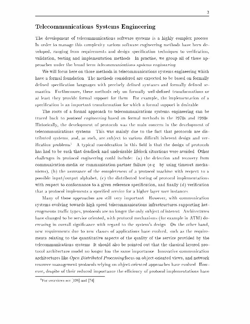
3Telecommunications Systems EngineeringThe development of telecommunications software systems is a highly complex process.In order to manage this complexity various software engineering methods have been de-veloped, ranging from requirements and design speci�cation techniques to veri�cation,validation, testing and implementation methods. In practise, we group all of these ap-proaches under the broad term telecommunications systems engineering.We will focus here on those methods in telecommunications systems engineering whichhave a formal foundation. The methods considered are expected to be based on formallyde�ned speci�cation languages with precisely de�ned syntaxes and formally de�ned se-mantics. Furthermore, these methods rely on formally well-de�ned transformations orat least they provide formal support for them. For example, the implementation of aspeci�cation is an important transformation for which a formal support is desirable.The roots of a formal approach to telecommunications systems engineering can betraced back to protocol engineering based on formal methods in the 1970s and 1980s.Historically, the development of protocols was the main concern in the development oftelecommunications systems. This was mainly due to the fact that protocols are dis-tributed systems, and, as such, are subject to various di�cult inherent design and ver-i�cation problems1. A typical consideration in this �eld is that the design of protocolshas had to be such that deadlock and undesirable lifelock situations were avoided. Otherchallenges in protocol engineering could include: (a) the detection and recovery fromcommunication-media or communication-partner failure (e.g. by using timeout mecha-nisms), (b) the assurance of the completeness of a protocol machine with respect to apossible input/output alphabet, (c) the distributed testing of protocol implementationswith respect to conformance to a given reference speci�cation, and �nally (d) veri�cationthat a protocol implements a speci�ed service for a higher layer user instances.Many of these approaches are still very important. However, with communicationsystems evolving towards high speed telecommunications infrastructures supporting het-erogeneous tra�c types, protocols are no longer the only subject of interest. Architectureshave changed to be service oriented, with protocol mechanisms (for example in ATM) de-creasing in overall signi�cance with regard to the system's design. On the other hand,new requirements due to new classes of applications have evolved, such as the require-ments relating to the quantitative aspects of the quality of the service provided by thetelecommunications systems. It should also be pointed out that the classical layered pro-tocol architecture model no longer has the same importance. Innovative communicationarchitectures like Open Distributed Processing focus on object-oriented views, and networkresource management protocols relying on object-oriented approaches have evolved. How-ever, despite of their reduced importance the e�ciency of protocol implementations have1For overviews see [108] and [74]

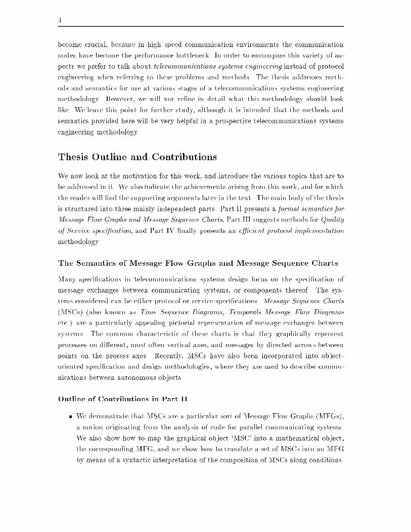
4become crucial, because in high speed communication environments the communicationnodes have become the performance bottleneck. In order to encompass this variety of as-pects we prefer to talk about telecommunications systems engineering instead of protocolengineering when referring to these problems and methods. The thesis addresses meth-ods and semantics for use at various stages of a telecommunications systems engineeringmethodology. However, we will not re�ne in detail what this methodology should looklike. We leave this point for further study, although it is intended that the methods andsemantics provided here will be very helpful in a prospective telecommunications systemsengineering methodology.Thesis Outline and ContributionsWe now look at the motivation for this work, and introduce the various topics that are tobe addressed in it. We also indicate the achievements arising from this work, and for whichthe reader will �nd the supporting arguments later in the text. The main body of the thesisis structured into three mainly independent parts. Part II presents a formal semantics forMessage Flow Graphs and Message Sequence Charts, Part III suggests methods for Qualityof Service speci�cation, and Part IV �nally presents an e�cient protocol implementationmethodology.The Semantics of Message Flow Graphs and Message Sequence ChartsMany speci�cations in telecommunications systems design focus on the speci�cation ofmessage exchanges between communicating systems, or components thereof. The sys-tems considered can be either protocol or service speci�cations. Message Sequence Charts(MSCs) (also known as Time Sequence Diagrams, Temporals Message Flow Diagramsetc.) are a particularly appealing pictorial representation of message exchanges betweensystems. The common characteristic of these charts is that they graphically representprocesses on di�erent, most often vertical axes, and messages by directed arrows betweenpoints on the process axes. Recently, MSCs have also been incorporated into object-oriented speci�cation and design methodologies, where they are used to describe commu-nications between autonomous objects.Outline of Contributions in Part II.� We demonstrate that MSCs are a particular sort of Message Flow Graphs (MFGs),a notion originating from the analysis of code for parallel communicating systems.We also show how to map the graphical object `MSC' into a mathematical object,the corresponding MFG, and we show how to translate a set of MSCs into an MFGby means of a syntactic interpretation of the composition of MSCs along conditions.

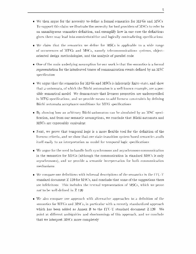
5� We then argue for the necessity to de�ne a formal semantics for MFGs and MSCs.To support this claim we illustrate the necessity for tool providers of MSCs to refer toan unambiguous semantics de�nition, and exemplify how in one case the de�nitionsgiven there may lead into counterintuitive and logically contradicting speci�cations.� We claim that the semantics we de�ne for MSCs is applicable to a wide rangeof occurrences of MFGs and MSCs, namely telecommunications systems, object-oriented design methodologies, and the analysis of parallel code.� One of the main underlying assumption for our work is that the semantics is a formalrepresentation for the interleaved traces of communication events de�ned by an MSCspeci�cation.� We argue that the semantics for MFGs and MSCs is inherently �nite-state, and showthat !-automata, of which the B�uchi automaton is a well-known example, are a pos-sible semantical model. We demonstrate that liveness properties are underspeci�edin MFG speci�cations, and we provide means to add liveness constraints by de�ningB�uchi automata acceptance conditions for MFG speci�cations.� By showing how an arbitrary B�uchi-automaton can be simulated by an MSC speci-�cation, and from our semantic assumptions, we conclude that B�uchi-automata andMSCs are expressibly equivalent.� Next, we prove that temporal logic is a more exible tool for the de�nition of theliveness criteria, and we show that our state-transition system based semantics availsitself easily to an interpretation as model for temporal logic speci�cations.� We argue for the need to handle both synchronous and asynchronous communicationin the semantics for MFGs (although the communication in standard MSCs is onlyasynchronous), and we provide a semantic interpretation for both communicationmechanisms.� We compare our de�nitions with informal descriptions of the semantics in the ITU-Tstandard document Z.120 for MSCs, and conclude that some of the suggestions thereare infelicitous. This includes the textual representation of MSCs, which we provenot to be well-de�ned in Z.120.� We also compare our approach with alternative approaches to a de�nition of thesemantics for MFGs and MSCs, in particular with a recently standardized approachwhich has been added as Annex B to the ITU-T standard document Z.120. Wepoint at di�erent ambiguities and shortcomings of this approach, and we concludethat we interpret MSCs more completely.

6 � We show that seemingly innocuous syntactic choices, in particular the cross-overof messages, can have implications on hidden assumptions on the behaviour of theenvironment. We criticise this because in our view when dealing with a very simpleand intuitive speci�cation style like MSCs what you see should be what you get.� As a consequence of the what you see is what you get requirement as well as of ourarguments for a �nite state semantics, we conclude that there are no queues involvedin the communications between processes.� Furthermore, we point out that the one-to-one communication relationship betweensending and receiving of messages (later in the text called `the property (*)') dis-tinguishes communications in MSCs from many other concurrent speci�cation tech-niques, like for example SDL.� Finally, we show that the unimpeded use of conditions leads to so-called non-localchoice situations, which can only be handled by using potentially unbounded historyvariables in the environment, or similar mechanisms. This contradicts both our�nite-state assumption, as well as our what you see is what you get requirement.Quality of Service Speci�cationTelecommunications Systems are evolving towards highly complex systems providing het-erogeneous services at very high communication speeds. A consequence of this develop-ment is that quantitative aspects of the quality of the service provided need to be spec-i�ed, and mechanisms for assuring their satisfaction need to be implemented. Examplesfor these requirements are delay bounds, delay jitter bounds, throughput rates and lossrates which are essential to video transmissions in multimedia applications. These sortsof requirements are often referred to as Quality of Service (QoS) requirements, and theyusually rely on real-time and probabilistic properties. The standard Formal DescriptionTechniques (FDTs) like Estelle, LOTOS and SDL, however, do not provide for expressingthese properties, therefore we investigate approaches for their speci�cation in Part III.Outline of Contributions in Part III.� We analyze the real-time mechanism in SDL, and we conjecture that it is unsuitableto specify real-time progress or bounded response properties, due to a lack of urgenceof events.� We show that it is possible to interpret SDL speci�cations as models for temporallogic formulas, and we provide a sketch of such an interpretation.� We de�ne the concept of complementary speci�cations, which are joint SDL/MSCand temporal logic speci�cations.

7� We then extend the interpretation to timed models and real-time temporal logics inorder to specify hard real-time constraints for SDL speci�cations.� Then we exemplify the application of these complementary speci�cations to thespeci�cation of some common real-time related quality of service requirements fortelecommunications services, to real-time related aspects of protocols, and to QoSmechanisms.E�cient Protocol ImplementationA further consequence of the evolution of telecommunications systems and in particularof the underlying optical transmission technology is that, as opposed to conventional com-munications systems, the performance bottleneck is no longer the transmission link, butinstead the protocol processing machine. This can be illustrated by a simple example:consider a standard workstation with a 32 bit architecture and a bus clock with a fre-quency of 25 MHz, then this yields a maximal data transfer rate inside the machine of800 Mbit/sec, even if the processor runs at a multiple of the bus clock frequency [121].This data transfer rate is easily exceeded by data transmission rates in broadband com-munication infrastructures like ATM. It is therefore imperative to have e�cient protocolimplementations available. In Part IV we therefore propose a method to transform the se-quential structure of operations inside the processes of an SDL speci�cations into optimizedrelaxed dependence graphs which serve as a basis for for e�cient parallel implementationsof the speci�ed protocol.Outline of Contributions in Part IV.� We show that it is ine�cient to implement SDL speci�cations in a `faithful' way bystructuring the implementation according to the structure of the speci�cation.� It is argued that the lack of explicit parallelism inside SDL speci�cations, the struc-turing of SDL speci�cations into processes, and the asynchronous inter-layer com-munication mechanism object to the e�cient direct implementation of SDL speci�-cations in a `faithful' way.� We suggest the construction of a multi-layer dependence graph of statements indi�erent layers of an SDL speci�cation. We transform this graph into a relaxeddependence graph, mainly by discarding sequential control ow dependences andretaining data dependences.� The relaxed dependence graph serves as a basis for the interpretation of di�erentprotocol implementation optimization methods, like combined execution of data ma-nipulation operations, and for a parallel execution.

8 � Depending on the target hardware and the resource constraints of individual op-erations this leads to a scheduling problem, which may be solved at compile- orrun-time.Acknowledgements. As already mentioned, a major part of the work in Part IV arosefrom collaboration with Philippe Oechslin, and is based on his and the author's joint ideathat control ow dependences need to be relaxed in order to allow for e�cient implemen-tations of the operations in a protocol stack. The ideas and concepts in Part IV due tocontributions made by Philippe are: the determination and derivation of a Common PathGraph, the Anticipation of the Comon Case, the notion of Auxiliary Dependences whichneed to be added to data dependences to form the Relaxed Dependence Graph, and theideas concerning a Scheduling of Operations in an implementation. The respective materialwill be published in [122].

Part IIThe Semantics of Message FlowGraphs and Message SequenceCharts

Chapter 1Introduction\Formalized methods : : : continue to rely on the intuitive understanding of thenotations and concepts employed: they may replace a possibly wooly naturallanguage description with, say, an apparently precise diagram { but the preci-sion is illusory if there is no underlying semantics giving a strict meaning tothe diagram." [133]The purpose of this part of the thesis is to give a precise formal semantics to a speci�-cation formalism often referred to as Message Flow Graphs (MFGs). Experience in bothacademic research and in industry has shown that MFGs lend themselves to easy picto-rial representation of inter-process communications, and they are consequently found intelecommunications, distributed, and object-oriented system design, and are frequentlyused in textbooks. Informally, they make helpful pictures, which are easy for the readerto relate to, and this undoubtedly accounts for their popularity.One type of MFG, is the Message Sequence Chart (MSC), de�ned in InternationalTelecommunications Union (ITU-T)1 Recommendation Z.120 [33]. MSCs provide a syn-tactically standardised description technique for telecommunications system design andvalidation. Throughout the remainder of this thesis, we shall refer to the ITU-T MSCstandard simply as Z.120.What Are MFGs and MSCs Good For? MFGs and MSCs describe process controlstructures and message exchanges of communicating processes. However they abstractfrom internal process computation. This distinguishes them from speci�cation languageslike SDL [32], Estelle [77] or LOTOS [78]. These languages specify the internal behaviourof communicating processes and the communication behaviour can only be inferred fromthe process code. Concludingly, one can say that MFGs and MSCs specify explicit com-munication behaviour while the process behaviour is implicit, whereas SDL, Estelle and1The former ITU standardization body CCITT has been renamed ITU-T in 1993.

12 1. IntroductionLOTOS specify the process behaviour explicitly while the communication behaviour is im-plicit. The system view represented by MFGs and MSCs can be helpful at all those stagesof the telecommunications systems engineering process at which an easy and graphicallyappealing representation of a system's communication behaviour is particularly helpful,as for example at early design stages, or in conformance testing. For a discussion of someoccurrences of MFGs and MSCs see Chapter 3.Why a Formal Semantics? Work on formal semantics of MSCs has often been criti-cised by claiming that MSC speci�cations only show(a) a partial view of the system behaviour, or(b) an intuitive and possibly inexact description of behaviour traces or scenarios,and that both points defeat the de�nition of an unambiguous, formal semantics. However,we are easily able to counter both of these points.� Firstly, our work does not focus on methodological aspects. MSCs are used widely(sometimes intuitively, sometimes formally) at various stages of the software engi-neering cycle for telecommunications systems, and, used in such a manner, MSCspeci�cations do describe system behaviours. Some opponents of a formal semanticsargue that MSC descriptions only represent `incomplete' traces of system behaviour.It remains unclear however, just what the completeness measure in this type of ar-gument is, and we have come to the conclusion that it is irrelevant. Indeed, weprovide a meaning to MSCs as they are given, independent of any particular con-text of application. However, we propose that the meaning we give is a canonicalinterpretation of MFGs and MSCs, and is thus applicable in any context.� Secondly, we propose that for MFGs and MSCs to have any use at all, a precisemeaning is indispensable. System speci�cation methods used in industry can be verydi�erent from those investigated by researchers. One might say that while commonindustrial methods are good at book-keeping, well-engineered and relatively easy toteach, they can be fuzzy in stating system properties. In contrast, mathematicalmethods such as those based on logic or automata are more precise and expressive,but require greater depth of mathematical or logical understanding to use. Webelieve there is value in bringing the precision of logic-based speci�cation methodsto existing industrial methods.Rigorous speci�cation methods such as Z, VDM, LOTOS, and the B Toolkit arealready �nding favor in industry. These methods seem to be following a path fromuse in academia to industrial research applications. In contrast, MFGs and MSCs areused in industry already, often informally. A precise semantics helps to illuminate

1. Introduction 13system features and clarify issues during system development, and is highly desirableand almost certainly essential when wanting to use MSCs or MFGs in the contextof system veri�cation, validation and testing. In particular, it enables MFGs andMSCs to be used in high reliability or safety-critical contexts, in which precision isof the essence.Motivation. Our motivation for this work came from two di�erent directions. We be-lieve that it is a touchstone of a worthwhile abstraction that it applies in di�erent contexts.� Firstly, it was demonstrated in [96] and [98] (summaries in [99], [97], with the com-plete material in [100]) that MFGs are very useful in deadlock and reachabilityanalyses of parallel code. The MFGs were rather simple, involving loops but nobranching. To extend the analysis, it became clear that some mechanism to keeptrack of branching was required.� Secondly, in apparently unrelated work, we wanted to provide a rigorous seman-tics for MSCs and Time Sequence Diagrams (TSDs) [81] in an telecommunicationssystems engineering context, and we found it convenient to base their semantic in-terpretation on MFGs2.Given that MFGs have proved useful in di�erent contexts, a natural next step is to de�nean unambiguous formal interpretation of each MFG, hence the present work.2In earlier publications we sometimes referred to ne/sig graphs, a special form of MFG.

Chapter 2What is a Message Flow Graph?MFGs are a graphical, intuitive method for describing partial message-passing interactionsbetween processes in communicating systems. They are frequently found in documentson design, validation and veri�cation, as well as in textbooks. They are frequently usedin describing aspects of telecommunications systems, and recently also gained importancein the description of communications in Object Models for object-oriented software devel-opment. One particularly important class of MFGs is that of Message Sequence Charts(MSCs), standardised by ITU-T Recommendation Z.120.Telecommunications protocol and service speci�cations as well as the speci�cation ofcommunications in Object Models are distinguished amongst general system speci�cationsby an emphasis on communication between processes rather than computation within aprocess, and by the relatively simple nature of the messages exchanged. Message FlowGraphs (MFGs) have been invented as a suitably abstract description method for this classof systems. They describe a system merely by the control structure of its processes, andby the structure of the inter-process message exchanges.Where are MFGs Found? MFGs have been de�ned in the context of static analysis ofparallel code. The currently most prominent area of application of MFGs is the design anddevelopment of telecommunications systems, where they can mainly be found as MSCsand TSDs. Recently, with the development of object-oriented design methods MFGs haveentered a new �eld of application. For more information on the occurrences of MFGs seeChapter 3.Systems Employing MFGs. MFGs have found their place in various software engi-neering methodologies and hence there are quite a number of commercial or non-commercialtools supporting MFGs that have been developed in academia and industry. Importantgroups of tools are those evolving from telecommunications systems engineering, and thoserelated to object models. We shall mention some tools and discuss requirements on one

16 2. What is a Message Flow Graph?a

!b ?bb

!d

?a!a

c

d

!c

?d

TopTopTop

?c

c

b

d

Bottom Bottom Bottom

a

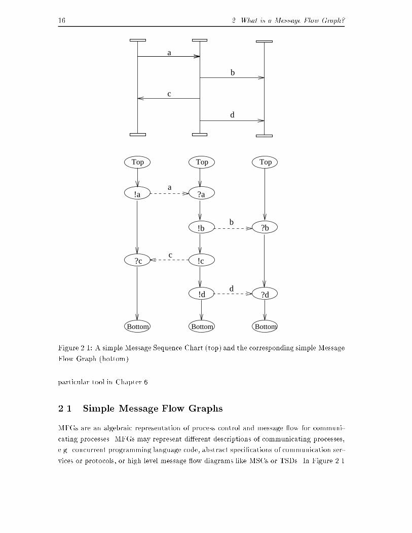
Figure 2.1: A simple Message Sequence Chart (top) and the corresponding simple MessageFlow Graph (bottom).particular tool in Chapter 6.2.1 Simple Message Flow GraphsMFGs are an algebraic representation of process control and message ow for communi-cating processes. MFGs may represent di�erent descriptions of communicating processes,e.g. concurrent programming language code, abstract speci�cations of communication ser-vices or protocols, or high level message ow diagrams like MSCs or TSDs. In Figure 2.1

2.1 Simple Message Flow Graphs 17the MFG on the bottom represents the intuitive picture on the top which is similar to anMSC or TSD. The MFG in this example does not contain conditions (a notion introducedfurther down), we therefore call it a simple MFG.In the picture on the top of Figure 2.1 processes are represented by vertical lines,and the signals sent between processes are represented by horizontal or sloping arrows.Communication is asynchronous. The junction between a vertical process line and ahorizontal signal line represents an event at which a signal of the type speci�ed is sentor received by the process. In each process axis, the events are temporally ordered fromtop to bottom, hence the ordering of events along a process axis is total. However, dueto the concurrent nature of the di�erent processes the picture describes a partial order ofthe communication events related to the sending and receiving of messages a; b; c and d.The message send1 and receive events are represented by the intersection of the messagearrows with the process lines. In the example, the �rst process sends a signal of type ato the second process, which upon reception sends a signal of type b to the third process,a signal of type c to the �rst process, and �nally a signal of type d to the third process.The system terminates when all processes have terminated.The MFG corresponding to this picture is on the bottom in the same Figure. The basicidea of the MFG is that it is represented by a graph structure which has an underlyingontology of message send and receive events represented as nodes. MFGs have twokinds of edges, next event (ne) and signal (sig) edges, representing explicit relations onthe nodes. The nodes are connected by solid arrows representing the next-event (ne)relation, indicating the next node in the same process (the process control), and dashedarrows corresponding to the signal (sig) relation, indicating from which node and to whichnode a message is passed. All nodes in an MFG, with the exception of the start andfinish nodes, must be connected to precisely one other node.The nodes (representing the events) are labeled with the event type. We use a variantof a common notation. The event node at the tail of a sig edge must be labeled with !a(send a message of type a), for some symbol `a' denoting the message type, and the eventnode at the head with ?a (receive a message of type a), for the same `a'. (In some uses,it might be preferred to label the sig edge with a and omit the node labels.) An MFG hasstart nodes (in the domain but not the range of the ne relation) labeled Top, and maybeend nodes (in the range but not the domain of ne) labeled Bottom2. We will present aformalisation of this informal de�nition of MFGs in Section 7.2.1We sometimes abuse notation mildly by using the phrase `message A' when we really mean `instanceof a message of type A', which is an awkward, although more accurate, phrase.2In later MFG examples we sometimes also write a lower-case letter within a node to allow us to referto that node in the text. These additional identifying letters do not occur in the MFG itself.

18 2. What is a Message Flow Graph?2.2 From MSCs to MFGsMSCs are graphical devices, whereas MFGs are mathematical objects (graphs). As thesemantics is based on the mathematical object we need to describe how to translate theformer into the latter (although some readers may consider this a pedantry).The translation is quite obvious. The MSC standard Z.120 de�nes notions like in-stances (the processes' control ows), message output and message input symbols. Z.120de�nes these symbols for both a graphical and a textual representation of MSCs.� In the graphical representation, an instance is represented by a vertical line, calledinstance axis. The instance axis may have horizontal or sloping arrows pointing awayfrom it or to it. We call the intersection of the departing arrow with an instanceaxis an output symbol, and the intersection of an incoming arrow and an instanceaxis an input symbol.� In the textual representation an instance is denoted by the keyword instance andcomprises the subsequent code until an endinstance symbol is reached. The corecode of an instance contains message input statements, denoted by keyword in, andmessage output statements, denoted by keyword out.To cover both representations (although we mainly use the graphical form in our examples)we will from here on only use the terms message input symbol and message outputsymbol, with the obvious meaning in the context of any chosen representation. We will nowsimply identify these symbols with the nodes in the MFG (representing the correspondingevents) and ensure that the MFG structure is consistent with the structure of the MSC.This means for example that the message input and message output symbols relatedto the message of type a in the MSC example in Figure 2.1 are mapped to a pair of nodesin the MFG so that this pair of send and receive nodes is in the sig relation of the MFG,and that it is labeled with signal type a. Furthermore, in order to represent the control ow of the left process in the corresponding MFG the node corresponding to the sendingof message a must be connected with a node which corresponds to the message inputsymbol related to a message of type c in the MSC, etc. We formalise this mapping inSection 7.2.2.2.3 Message Flow Graphs with ConditionsTo this end, we de�ne conditions in MFGs. Conditions are global labels on process axes3.We also de�ne a composition operation which allows MFGs to be `joined' at these con-ditions. This composition is a purely syntactic operation on MFGs. By allowing more3The term condition has been introduced in Z.120. A condition is a syntactic label and should not bemisunderstood as a condition in a logical sense.

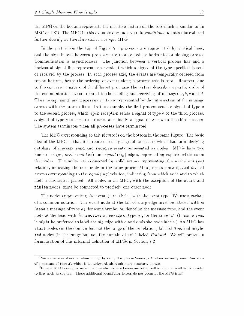
2.3 Message Flow Graphs with Conditions 19C

C

a

I

a!a ?a

T1 T2

y

w x

zFigure 2.2: MSC I and corresponding MFG Ithan one possible joining, one obtains the e�ect of non-deterministic choice in MFGs (butconditionals de�ned on the values of state predicates are still not possible). By writingthe same condition at the beginning as well as the end of an MFG, one obtains non-terminating-loop-like behavior. This allows us to de�ne the (partial) use of conditions asconceived in Z.120, but as we will note in Section 8.2, unrestricted use of conditions seemsto entail that the environment has powerful implicit properties which are not explicit inan MFG speci�cation.The simple MSC and MFG example in Figure 2.1 does not show looping behaviorof MFGs, as seen in Figures 2.2, 2.3, 2.4, and 2.5. A loop in an MSC speci�cation iscaused by conditions, as described below. A loop in an MFG is simply a cycle in thenext-event (solid-arrow) relation. In such a case, the nodes in an MFG may no longerrepresent events, since in a trace of the MFG they are or may be traversed multiple times.Thus nodes in an MFG should be properly thought of in the manner of statements of aprogramming language, which may be executed multiple times, each execution of whichis a message-passing event.Whereas the MFGs in Figures 2.2 and 2.3 are simple non-branching non-nested loopstructures, Figure 2.7 shows MFGs with conditions, represented by the diamond-shapednodes, corresponding to the MSC speci�cation in Figure 2.6. The idea is that control thatarrives at a condition node may continue in another MFG from a condition node withan identical label, as if the MFGs were `joined' at these condition nodes. Thus di�erentMFGs starting with identical condition nodes provide di�erent ways to continue control4.We now elaborate two reasons for incorporating looping and branching structures intoMFGs: the need to represent iterations and non-determinism in MFG speci�cations.2.3.1 Iterations in MFGs4We are not totally convinced that this can be done without di�culty, as noted in Section 8.2. Never-theless, we provide in Section 7.4 the apparatus to e�ect it.

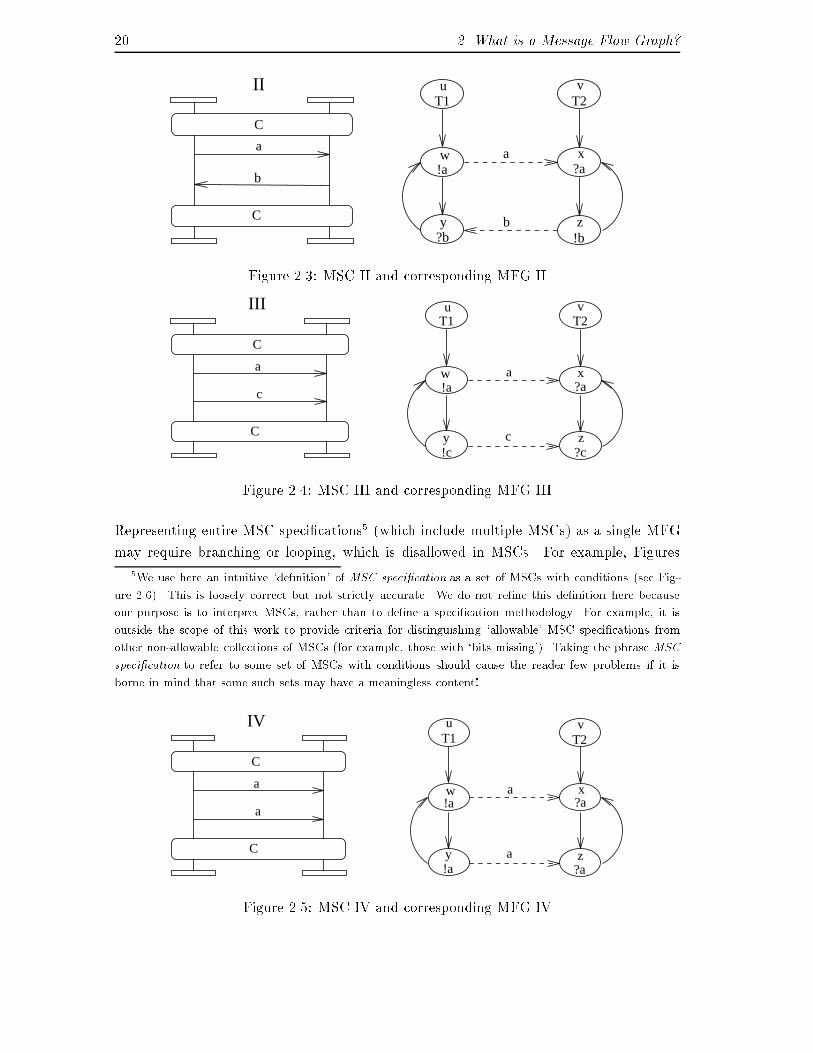
20 2. What is a Message Flow Graph?C

C

a

b

II

b

a!a ?a

T2T1

?b !bzy

xw

vu

Figure 2.3: MSC II and corresponding MFG IIC

C

a

c

III

a

c

T1 T2

!a ?a

?c!c

u v

x

y z

wFigure 2.4: MSC III and corresponding MFG IIIRepresenting entire MSC speci�cations5 (which include multiple MSCs) as a single MFGmay require branching or looping, which is disallowed in MSCs. For example, Figures5We use here an intuitive `de�nition' of MSC speci�cation as a set of MSCs with conditions (see Fig-ure 2.6). This is loosely correct but not strictly accurate. We do not re�ne this de�nition here becauseour purpose is to interpret MSCs, rather than to de�ne a speci�cation methodology. For example, it isoutside the scope of this work to provide criteria for distinguishing `allowable' MSC speci�cations fromother non-allowable collections of MSCs (for example, those with `bits missing'). Taking the phrase MSCspeci�cation to refer to some set of MSCs with conditions should cause the reader few problems if it isborne in mind that some such sets may have a meaningless content!C

C

a

IV

a

a

a

T1 T2

?a!a

u v

w x

y z!a ?aFigure 2.5: MSC IV and corresponding MFG IV

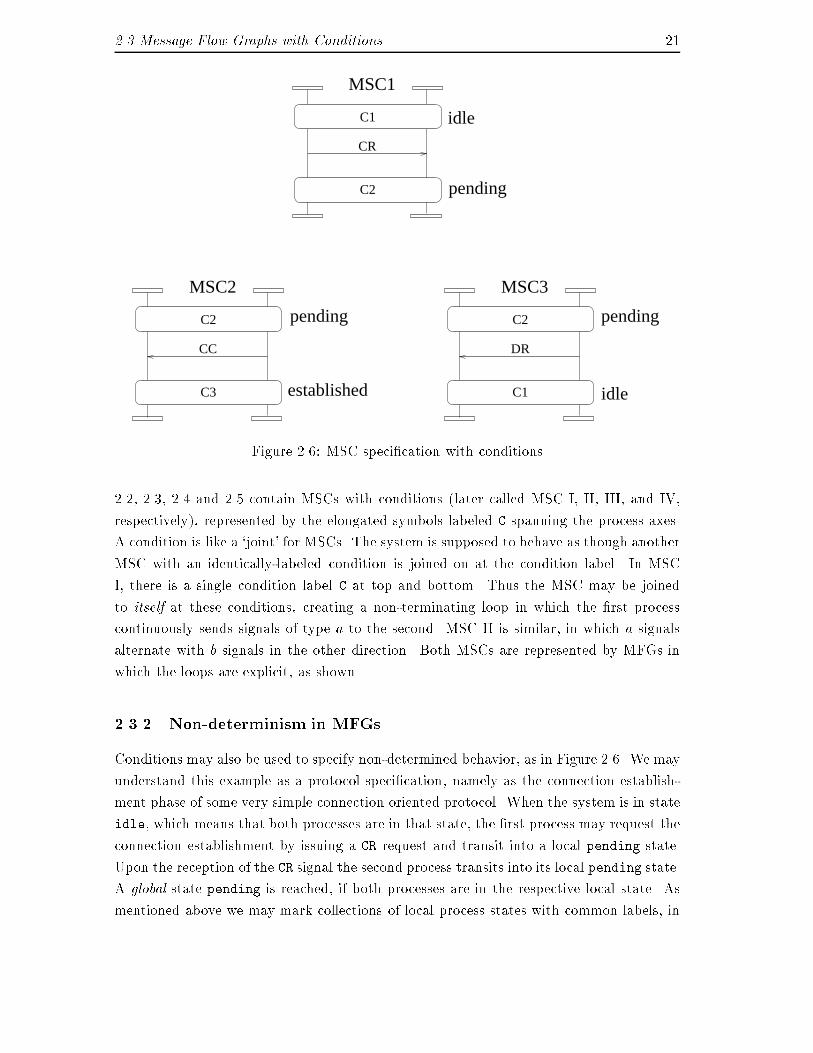
2.3 Message Flow Graphs with Conditions 21idle

DR

MSC3

C2 pendingC2

C3

CC

pending

established C1

MSC2

MSC1

C2

C1

CR

pending

idle

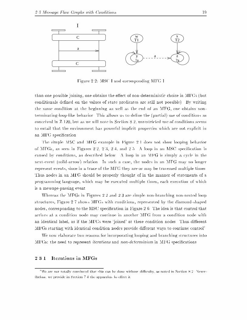
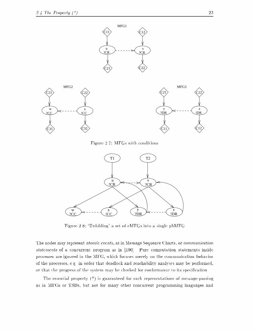
Figure 2.6: MSC speci�cation with conditions2.2, 2.3, 2.4 and 2.5 contain MSCs with conditions (later called MSC I, II, III, and IV,respectively), represented by the elongated symbols labeled C spanning the process axes.A condition is like a `joint' for MSCs. The system is supposed to behave as though anotherMSC with an identically-labeled condition is joined on at the condition label. In MSCI, there is a single condition label C at top and bottom. Thus the MSC may be joinedto itself at these conditions, creating a non-terminating loop in which the �rst processcontinuously sends signals of type a to the second. MSC II is similar, in which a signalsalternate with b signals in the other direction. Both MSCs are represented by MFGs inwhich the loops are explicit, as shown.2.3.2 Non-determinism in MFGsConditions may also be used to specify non-determined behavior, as in Figure 2.6. We mayunderstand this example as a protocol speci�cation, namely as the connection establish-ment phase of some very simple connection oriented protocol. When the system is in stateidle, which means that both processes are in that state, the �rst process may request theconnection establishment by issuing a CR request and transit into a local pending state.Upon the reception of the CR signal the second process transits into its local pending state.A global state pending is reached, if both processes are in the respective local state. Asmentioned above we may mark collections of local process states with common labels, in

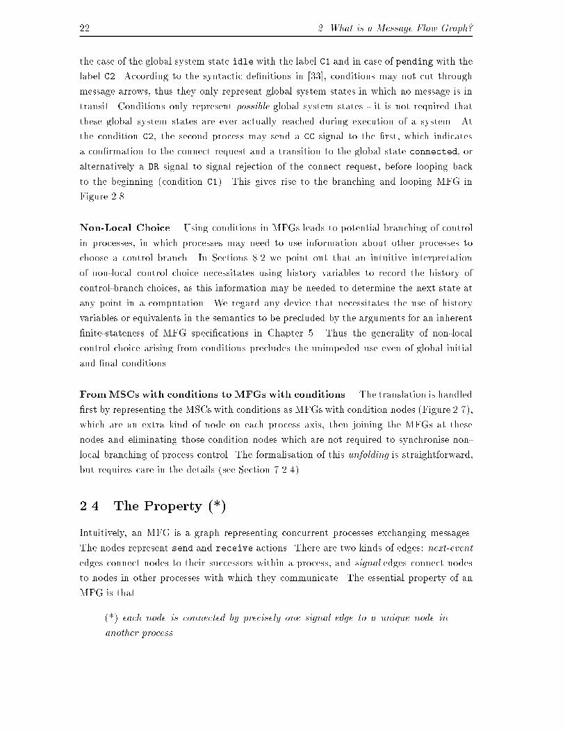
22 2. What is a Message Flow Graph?the case of the global system state idle with the label C1 and in case of pending with thelabel C2. According to the syntactic de�nitions in [33], conditions may not cut throughmessage arrows, thus they only represent global system states in which no message is intransit. Conditions only represent possible global system states - it is not required thatthese global system states are ever actually reached during execution of a system. Atthe condition C2, the second process may send a CC signal to the �rst, which indicatesa con�rmation to the connect request and a transition to the global state connected, oralternatively a DR signal to signal rejection of the connect request, before looping backto the beginning (condition C1). This gives rise to the branching and looping MFG inFigure 2.8.Non-Local Choice. Using conditions in MFGs leads to potential branching of controlin processes, in which processes may need to use information about other processes tochoose a control branch. In Sections 8.2 we point out that an intuitive interpretationof non-local control choice necessitates using history variables to record the history ofcontrol-branch choices, as this information may be needed to determine the next state atany point in a computation. We regard any device that necessitates the use of historyvariables or equivalents in the semantics to be precluded by the arguments for an inherent�nite-stateness of MFG speci�cations in Chapter 5. Thus the generality of non-localcontrol choice arising from conditions precludes the unimpeded use even of global initialand �nal conditions.FromMSCs with conditions to MFGs with conditions. The translation is handled�rst by representing the MSCs with conditions as MFGs with condition nodes (Figure 2.7),which are an extra kind of node on each process axis, then joining the MFGs at thesenodes and eliminating those condition nodes which are not required to synchronise non-local branching of process control. The formalisation of this unfolding is straightforward,but requires care in the details (see Section 7.2.4).2.4 The Property (*).Intuitively, an MFG is a graph representing concurrent processes exchanging messages.The nodes represent send and receive actions. There are two kinds of edges: next-eventedges connect nodes to their successors within a process, and signal edges connect nodesto nodes in other processes with which they communicate. The essential property of anMFG is that(*) each node is connected by precisely one signal edge to a unique node inanother process.

2.4 The Property (*). 23C21 C22

C32C31

?CCw

!CCx

MFG2

C12C11

C22C21

!CR ?CRu v

MFG1

C21 C22

C11 C12

?DR !DRy z

MFG3

Figure 2.7: MFGs with conditionsT1

!CR ?CR

?CC !CC ?DR

u v

!DRx yw z

T2

Figure 2.8: `Unfolding' a set of cMFGs into a single pbMFGThe nodes may represent atomic events, as in Message Sequence Charts, or communicationstatements of a concurrent program as in [100]. Pure computation statements insideprocesses are ignored in the MFG, which focuses merely on the communication behaviorof the processes, e.g. in order that deadlock and reachability analyses may be performed,or that the progress of the system may be checked for conformance to its speci�cation.The essential property (*) is guaranteed for such representations of message-passingas in MFGs or TSDs, but not for many other concurrent programming languages and

24 2. What is a Message Flow Graph?speci�cation techniques6. However, for other structures such as processes with a singlenon-terminating loop, proving the existence of an MFG describing the progress of thesystem can be non-trivial. An algorithm for constructing a minimal MFG from a collectionof concurrent so-called loop processes was given in [100].2.5 Message Flow Graphs: an Abstract SyntaxDi�erent types of communication can have contrasting features, for example synchronousor asynchronous, channelled or broadcast, �nitely or in�nitely bu�ered, reliable or unre-liable. Similarly, processes may be deterministic or non-deterministic, including parallelconstructions or not, terminating or non-terminating. Because an MFG may be used todescribe a mathematical syntax for the message-passing features of di�erent speci�cationmethods, the graph is neutral with regard to the meaning of signal edges, the types of com-munication, or the control structure of processes. However, it does determine staticallythe sender and recipients of each communication (c.f. property (*)). Thus it is an abstractsyntax: a syntax because it encodes only minimal semantic assumptions, and abstract be-cause it abstracts from the details of the syntax of any speci�c application. The semanticsarises from how the MFG is interpreted, as a particular kind of global state transitionsystem. One major purpose of the MFG is to be able to derive a single MFG, wherepossible, from a collection of simpler descriptions of communicating processes. As seenabove, for MSCs such a collection cannot be represented by a single MSC if the collectiondescribes looping behavior of any sort. Representing a collection of MFGs with conditionsas a single MFG without conditions (by means of the unfolding construction) enables useventually to de�ne the global state transitions and thus the automaton corresponding toa speci�cation.2.6 Overview of the MFG SemanticsIn Chapter 3 we present some occurrences of MFGs and MSCs, namely their occurrence inthe description of telecommunications systems (Section 3.1), in the analysis of parallel code(Section 3.2), and in object-oriented system analysis and design methodologies (Section3.3).We then specify our requirements for the semantics (see Chapter 4). These are mostimportantly that we use interleaved traces of message events, that the semantics is �nite-state, that liveness is underspeci�ed in MFGs and thus deserves special treatment, andthat we include the handling of synchronous communication. In Chapter 5 we elaborateour arguments for a �nite-state semantics. We further motivate our requirements on6Note that in SDL one OUTPUT(X) statement can be matched by many INPUT(X) statements.

2.6 Overview of the MFG Semantics 25the semantic with a discussion of industrial tools employing MSCs, in particular on theGEODE toolset, in Chapter 6.Chapter 7 contains the main part of the semantics de�nition. In Sections 7.3 and 7.4we obtain a global state transition graph (GSTG) from an MFG. A GSTG is like a �nite-state automaton but lacks de�nition of end-states. We consider end-state de�nitions inSection 7.5. Each possible end-state de�nition gives a B�uchi automaton. The MFG spec-i�cation under-de�nes the resulting automaton, in that end-state de�nitions are relatedto di�erent safety and liveness properties that one might wish to require as additions tothe speci�cation. We show in Section 7.6 how this may be done via a connection withtemporal logic, and we specify liveness properties for MFG speci�cations using temporallogic formulas there. We discuss some properties expressed in temporal logic which allMFGs satisfy, and some potentially desirable ones which some MFGs might be requiredto satisfy in some uses, in Section 7.8. We then show in Section 7.9 how synchronouscommunication can be accommodated along with asynchronous communication in MFGs,and give some reasons why this may be desired. We also note that the occurrence ofsynchronous communication in an MFG can simplify the liveness analysis. In Section 7.10we show how to simulate an arbitrary B�uchi automaton with an MFG speci�cation, andconclude that MFGs are expressively equivalent to B�uchi automata.In Chapter 8 we scrutinize the semantics of MFGs. In particular, we show that theunimpeded use of conditions leads to the need of history variables of unbounded size, thusdefeating our �nite-state assumption. Furthermore, we show that crossing message arrowscan cause undesirable implicit assumptions on the behaviour of the environment, thatMFGs can `count', and that liveness properties are better expressed by using TemporalLogic than by the use of acceptance conditions for B�uchi automata.In Chapter 9 we discuss the relation of our MFG semantics work to the MSC Z.120standard document, including a description of the extent to which our work covers theMSC language as de�ned in Z.120. In Chapter 10 we discuss alternative approachesto a semantics for MSCs. Recently, a process algebra based semantics for MSCs hasbeen standardized and added as Annex B to the Z.120 standard document. We o�er acomparison of our approach with the standard in Section 10.1.We suggest that readers primarily interested in the technical construction of our se-mantics directly proceed to Chapter 7.

Chapter 3Occurrences of Message FlowGraphsWe discuss and give examples for the most important occurrences of MFGs: in telecom-munications systems design, in the analysis of parallel code, and in object models.3.1 Telecommunications Systems DescriptionThe most prominent use of MFGs is in telecommunication systems design, in particularwhen specifying communication protocols and services. Most frequently, MFGs occur asMSCs or TDGs, both standardized graphical description methods (see [33] and [81]).Many examples of MFGs can be found in textbooks on database systems and computernetworks [140], where the use is mainly informal. In [147], where they are called primitivesequences, MFGs are used in the design of telecommunications systems. In industrialapplication contexts, MFGs are central to the work in [40] where they are called temporalmessage ow diagrams, and in [138] where they are called MSCs. For further use inindustry see [41]. MFGs are also used in telecommunications standards, see for example[30] and [31].As MFGs are widely accepted and reported in connection with telecommunicationssystems engineering, no particular examples are introduced here. However, the MFGexamples used in this thesis (e.g. Figures 2.1 and 2.6) contain typical uses of MFGs intelecommunications.3.2 Analysis of Parallel CodeMFGs were introduced in [96] as a means of analysing parallel code, in order to performdeadlock analysis and other optimisation at compile time. Analysis based on MFGs maybe found in [97], [99], and [100].

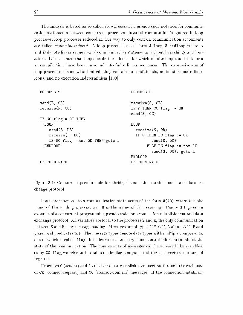
28 3. Occurrences of Message Flow GraphsThe analysis is based on so-called loop processes, a pseudo-code notation for communi-cation statements between concurrent processes. Internal computation is ignored in loopprocesses, loop processes reduced in this way to only contain communication statementsare called commstat-reduced. A loop process has the form A loop B endloop where Aand B denote linear sequences of communication statements without branchings and iter-ations. It is assumed that loops inside these blocks for which a �nite loop count is knownat compile time have been unwound into �nite linear sequences. The expressiveness ofloop processes is somewhat limited, they contain no conditionals, no indeterminate �niteloops, and no execution indeterminism [100].PROCESS S PROCESS Rsend(R, CR) receive(S, CR)receive(R, CC) IF P THEN CC.flag := OKsend(S, CC)IF CC.flag = OK THENLOOP LOOPsend(R, DR) receive(S, DR)receive(R, DC) IF Q THEN DC.flag := OKIF DC.flag = not OK THEN goto L send(S, DC)ENDLOOP ELSE DC.flag := not OKsend(S, DC); goto LENDLOOPL: TERMINATE L: TERMINATEFigure 3.1: Concurrent pseudo code for abridged connection establishment and data ex-change protocolLoop processes contain communication statements of the form W(AB) where A is thename of the sending process, and B is the name of the receiving. Figure 3.1 gives anexample of a concurrent programming pseudo code for a connection establishment and dataexchange protocol. All variables are local to the processes S and R, the only communicationbetween S and R is by message passing. Messages are of types CR;CC;DR and DC. P andQ are local predicates to R. The message types denote data types with multiple components,one of which is called flag. It is designated to carry some control information about thestate of the communication. The components of messages can be accessed like variables,so by CC.flag we refer to the value of the ag component of the last received message oftype CC.Processes S (sender) and R (receiver) �rst establish a connection through the exchangeof CR (connect-request) and CC (connect-con�rm) messages. If the connection establish-

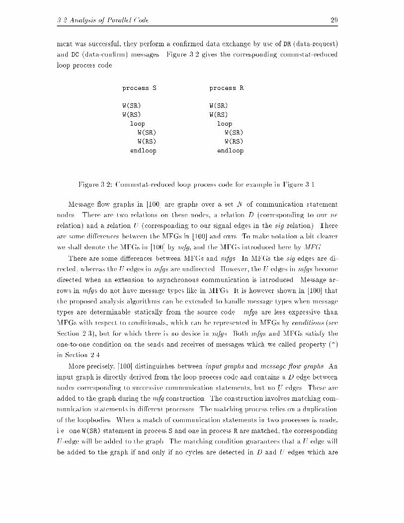
3.2 Analysis of Parallel Code 29ment was successful, they perform a con�rmed data exchange by use of DR (data-request)and DC (data-con�rm) messages. Figure 3.2 gives the corresponding commstat-reducedloop process code. process S process RW(SR) W(SR)W(RS) W(RS)loop loopW(SR) W(SR)W(RS) W(RS)endloop endloopFigure 3.2: Commstat-reduced loop process code for example in Figure 3.1.Message ow graphs in [100] are graphs over a set N of communication statementnodes. There are two relations on these nodes, a relation D (corresponding to our nerelation) and a relation U (corresponding to our signal edges in the sig relation). Thereare some di�erences between the MFGs in [100] and ours. To make notation a bit clearerwe shall denote the MFGs in [100] by mfg, and the MFGs introduced here by MFG.There are some di�erences between MFGs and mfgs. In MFGs the sig edges are di-rected, whereas the U edges in mfgs are undirected. However, the U edges in mfgs becomedirected when an extension to asynchronous communication is introduced. Message ar-rows in mfgs do not have message types like in MFGs. It is however shown in [100] thatthe proposed analysis algorithms can be extended to handle message types when messagetypes are determinable statically from the source code. mfgs are less expressive thanMFGs with respect to conditionals, which can be represented in MFGs by conditions (seeSection 2.3), but for which there is no device in mfgs. Both mfgs and MFGs satisfy theone-to-one condition on the sends and receives of messages which we called property (*)in Section 2.4.More precisely, [100] distinguishes between input graphs and message ow graphs. Aninput graph is directly derived from the loop process code and contains a D edge betweennodes corresponding to successive communication statements, but no U edges. These areadded to the graph during the mfg construction. The construction involves matching com-munication statements in di�erent processes. The matching process relies on a duplicationof the loopbodies. When a match of communication statements in two processes is made,i.e. one W(SR) statement in process S and one in process R are matched, the correspondingU -edge will be added to the graph. The matching condition guarantees that a U edge willbe added to the graph if and only if no cycles are detected in D and U edges which are

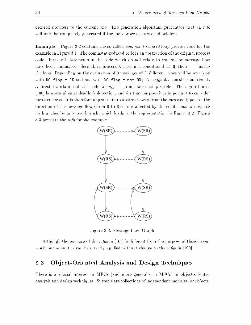
30 3. Occurrences of Message Flow Graphsordered previous to the current one. The generation algorithm guarantees that an mfgwill only be completely generated if the loop processes are deadlock-free.Example. Figure 3.2 contains the so called commstat-reduced loop process code for theexample in Figure 3.1. The commstat-reduced code is an abstraction of the original processcode. First, all statements in the code which do not relate to control- or message owhave been eliminated. Second, in process R there is a conditional if Q then ... insidethe loop. Depending on the evaluation of Q messages with di�erent types will be sent (onewith DC.flag = OK and one with DC.flag = not OK). As mfgs do contain conditionalsa direct translation of this code to mfgs is prima facie not possible. The algorithm in[100] however aims at deadlock detection, and for that purpose it is important to considermessage ows. It is therefore appropriate to abstract away from the message type. As thedirection of the message ow (from R to S) is not a�ected by the conditional we replaceits branches by only one branch, which leads to the representation in Figure 3.2. Figure3.3 presents the mfg for the example.W(SR) W(SR)

W(SR) W(SR)

W(RS) W(RS)

W(RS) W(RS)Figure 3.3: Message Flow Graph.Although the purpose of the mfgs in [100] is di�erent from the purpose of those in ourwork, our semantics can be directly applied without change to the mfgs in [100].3.3 Object-Oriented Analysis and Design TechniquesThere is a special interest in MFGs (and more generally in MSCs) in object-orientedanalysis and design techniques. Systems are collections of independent modules, or objects.

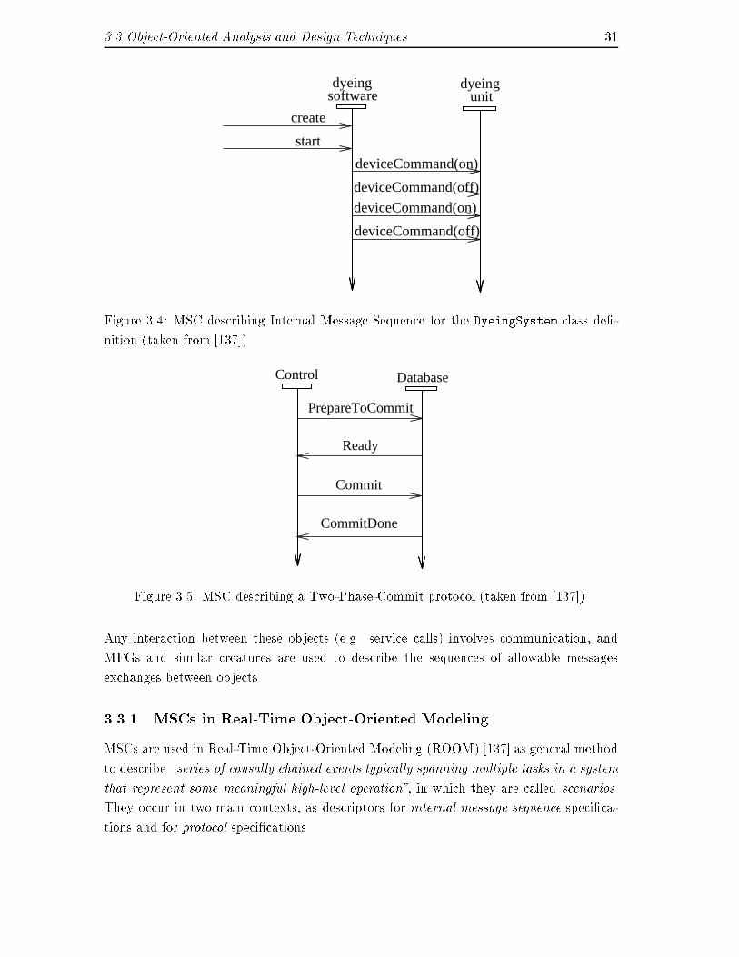
3.3 Object-Oriented Analysis and Design Techniques 31create

start

unitdyeing

softwaredyeing

deviceCommand(on)

deviceCommand(off)

deviceCommand(on)

deviceCommand(off)Figure 3.4: MSC describing Internal Message Sequence for the DyeingSystem class de�-nition (taken from [137]).PrepareToCommit

Control Database

CommitDone

Commit

Ready

Figure 3.5: MSC describing a Two-Phase-Commit protocol (taken from [137]).Any interaction between these objects (e.g. service calls) involves communication, andMFGs and similar creatures are used to describe the sequences of allowable messagesexchanges between objects.3.3.1 MSCs in Real-Time Object-Oriented ModelingMSCs are used in Real-Time Object-Oriented Modeling (ROOM) [137] as general methodto describe \series of causally chained events typically spanning multiple tasks in a systemthat represent some meaningful high-level operation", in which they are called scenarios.They occur in two main contexts, as descriptors for internal message sequence speci�ca-tions and for protocol speci�cations.

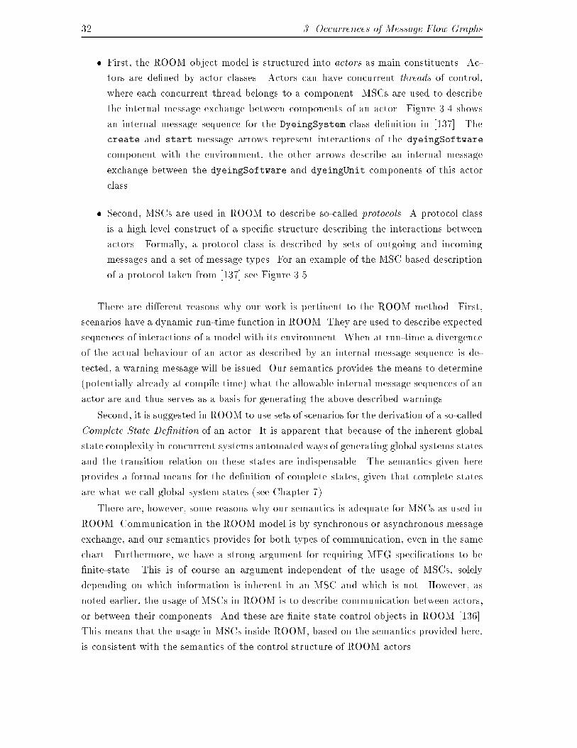
32 3. Occurrences of Message Flow Graphs� First, the ROOM object model is structured into actors as main constituents. Ac-tors are de�ned by actor classes. Actors can have concurrent threads of control,where each concurrent thread belongs to a component. MSCs are used to describethe internal message exchange between components of an actor. Figure 3.4 showsan internal message sequence for the DyeingSystem class de�nition in [137]. Thecreate and start message arrows represent interactions of the dyeingSoftwarecomponent with the environment, the other arrows describe an internal messageexchange between the dyeingSoftware and dyeingUnit components of this actorclass.� Second, MSCs are used in ROOM to describe so-called protocols. A protocol classis a high level construct of a speci�c structure describing the interactions betweenactors. Formally, a protocol class is described by sets of outgoing and incomingmessages and a set of message types. For an example of the MSC based descriptionof a protocol taken from [137] see Figure 3.5.There are di�erent reasons why our work is pertinent to the ROOM method. First,scenarios have a dynamic run-time function in ROOM. They are used to describe expectedsequences of interactions of a model with its environment. When at run-time a divergenceof the actual behaviour of an actor as described by an internal message sequence is de-tected, a warning message will be issued. Our semantics provides the means to determine(potentially already at compile time) what the allowable internal message sequences of anactor are and thus serves as a basis for generating the above described warnings.Second, it is suggested in ROOM to use sets of scenarios for the derivation of a so-calledComplete State De�nition of an actor. It is apparent that because of the inherent globalstate complexity in concurrent systems automated ways of generating global systems statesand the transition relation on these states are indispensable. The semantics given hereprovides a formal means for the de�nition of complete states, given that complete statesare what we call global system states (see Chapter 7).There are, however, some reasons why our semantics is adequate for MSCs as used inROOM. Communication in the ROOM model is by synchronous or asynchronous messageexchange, and our semantics provides for both types of communication, even in the samechart. Furthermore, we have a strong argument for requiring MFG speci�cations to be�nite-state. This is of course an argument independent of the usage of MSCs, solelydepending on which information is inherent in an MSC and which is not. However, asnoted earlier, the usage of MSCs in ROOM is to describe communication between actors,or between their components. And these are �nite state control objects in ROOM [136].This means that the usage in MSCs inside ROOM, based on the semantics provided here,is consistent with the semantics of the control structure of ROOM actors.

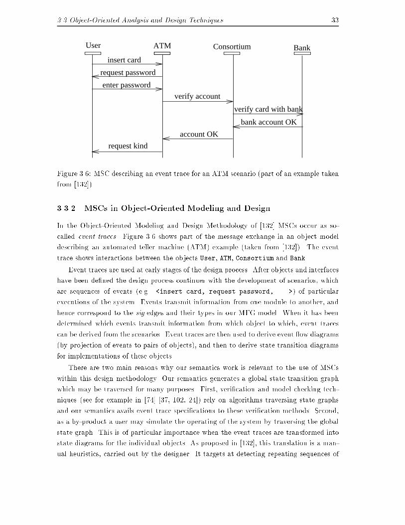
3.3 Object-Oriented Analysis and Design Techniques 33User ATM Consortium Bank

enter password

request password

insert card

verify account

account OK

request kind

verify card with bank

bank account OKFigure 3.6: MSC describing an event trace for an ATM scenario (part of an example takenfrom [132]).3.3.2 MSCs in Object-Oriented Modeling and DesignIn the Object-Oriented Modeling and Design Methodology of [132] MSCs occur as so-called event traces. Figure 3.6 shows part of the message exchange in an object modeldescribing an automated teller machine (ATM) example (taken from [132]). The eventtrace shows interactions between the objects User, ATM, Consortium and Bank.Event traces are used at early stages of the design process. After objects and interfaceshave been de�ned the design process continues with the development of scenarios, whichare sequences of events (e.g. <insert card, request password, ...>) of particularexecutions of the system. Events transmit information from one module to another, andhence correspond to the sig edges and their types in our MFG model. When it has beendetermined which events transmit information from which object to which, event tracescan be derived from the scenarios. Event traces are then used to derive event ow diagrams(by projection of events to pairs of objects), and then to derive state transition diagramsfor implementations of these objects.There are two main reasons why our semantics work is relevant to the use of MSCswithin this design methodology. Our semantics generates a global state transition graphwhich may be traversed for many purposes. First, veri�cation and model checking tech-niques (see for example in [74] [37, 102, 24]) rely on algorithms traversing state graphsand our semantics avails event trace speci�cations to these veri�cation methods. Second,as a by-product a user may simulate the operating of the system by traversing the globalstate graph. This is of particular importance when the event traces are transformed intostate diagrams for the individual objects. As proposed in [132], this translation is a man-ual heuristics, carried out by the designer. It targets at detecting repeating sequences of

34 3. Occurrences of Message Flow Graphsevents in order to detect potential loops in the object's control ow, and thus to deter-mine potential system states of individual objects. This step can be greatly enhanced bya simulation of the systems execution. Also, having a precise mathematical description ofwhat the event trace means helps in automating this manual task.

Chapter 4Requirements for the SemanticsWe now discuss our requirements for the MFG semantics. These are mainly, that we con-sider our semantics to be a determination of the interleaved sequences of communicationevents speci�ed by an MFG, that they be �nite-state, that liveness properties are under-speci�ed in MFGs and that therefore they deserve special treatment, that the complexityentailed by our semantics is not devastating, and that we handle both synchronous andasynchronous communications.4.1 Traces of Message Events are InterleavingsWe consider a semantics to be a precise determination of which execution traces a descrip-tion allows. Since we focus only on communication events, we take trace to mean traceof communication events only. Internal process computation is ignored, although it caneasily be added if desired. An interleaving model is one in which a trace is an interleavingof all observable atomic message-passing events of the system which is consistent with thelinear ordering of events within each process, from the point of view of a global observer.Interleaving models are used for many important speci�cation styles, including TLA [101],CSP [68], and LOTOS [78]. Taking traces of message passing events to be interleavingsis consistent with industrial use of MFGs. MSCs are often used for talking about frag-ments of tests, as they are in GEODE [6]. Taking traces to be interleavings of events isconsistent with the standard test de�nition language TTCN [79]. Thus we take traces tobe interleavings of atomic communication events.4.2 Finite-State SemanticsEven if it is assumed that there is only a �nite number of possible control states withrespect to messages, it nevertheless might be possible, if communication is asynchronous,for there to be an unbounded number of messages in the system (i.e. sent but not received).

36 4. Requirements for the SemanticsThus it is not immediately obvious that there are a �nite number of global communicationstates if one includes the messages in the system as well as the process control predicates.However, we shall argue in Section 5.6 that provided that the global state assumptionis satis�ed, and traces are interleavings, there are only �nitely many global states withrespect to the message-passing behavior of the system described by an MFG. Thus wemay de�ne a global �nite-state automaton, whose accepted language is identical with theset of system traces described by the MFG.Besides this argument which is particular to MFGs, justi�cation for a �nite-state re-quirement in general for telecommunications system speci�cations may be found in [74].The primary advantage for �nite-state interpretations is that reasonable veri�cation andvalidation techniques may be applied. There are many practical techniques for analysisand veri�cation of �nite-state systems ([37, 102, 43] as well as [74]). Such methods canexhibit a high degree of automation. They have been used successfully to validate systemswith up to 1014 states [42] by exhaustive state search, and up to 1020 states are beingconsidered [29].In contrast, non-�nite-state methods usually employ theorem-proving techniques whichare comparatively human-labor-intensive, are often research vehicles, and are currentlylimited in practical use. [91] argues for mixing the two sorts of techniques to obtain theadvantages of both. The authors use COSPAN and TLA to verify a hardware multiplierdesign. As of the time of writing, the state-of-the-art in practical telecommunicationssystem veri�cation and validation is �nite-statecraft.One consequence of �nite-stateliness is that MSCs, even those sets of MSCs with con-ditions (see below) that describe in�nite traces, exhibit only �nitely many global states.As we stated above, alternative proposals for the semantics of MSCs such as [134, 48, 64]do not de�ne the semantics of composed MSCs, and therefore provide much less cover-age than our semantics described in this document. Even if they did, our argument for�nite-stateliness indicates that since the states of the system may be enumerated, thesealternative approaches based on non-�nite-state methods need to argue their case on tech-nical grounds of greater e�ciency, or maybe on aesthetic grounds, but no evidence has yetbeen given that either of these pertain. We will elaborate the �nite-stateness requirementin our semantics in some more detail in Chapter 5.4.3 Liveness ConditionsGiven that a system is described by a �nite state-transition graph, there is nevertheless aquestion as to whether all traces through this graph are acceptable traces of the system, orwhether only a subset of them are. With asynchronous communication, a means is requiredfor expressing liveness and safety assumptions in addition to the basic vocabulary of MFGs,argued in Section 7.5 and solved in Section 7.6. In order to facilitate the expression of a

4.4 B�uchi- and Other !-Automata. 37wider array of liveness properties, it is necessary to go beyond the Global State TransitionGraph (GSTG) to consider which traces through the graph are allowed by the description(along with the liveness properties) and which are not. A standard way to express theseconditions is to consider the GSTG as providing most of the de�nition of an !-automaton,lacking only an end-state de�nition, and to provide that end-state de�nition.However, when communication is synchronous, the expression of safety and livenessare much simpli�ed, as noted in Section 7.9, and any non-�nite-state semantics for thiscase would be contrived. If one is de�ning a speci�cation method, this would provide agood reason for preferring synchronous communication primitives, as argued in [68, 119].However, MSCs as they are normally used utilise asynchronous message-passing.4.4 B�uchi- and Other !-Automata.Since traces may be in�nite, a �nite-state semantics requires use of a �nite-state automatonwhich accepts in�nite strings. This is the class of so-called !-automata [143] of which theB�uchi automaton is probably the most well-known. B�uchi automata have been used inthe determination of safety and liveness properties of distributed systems [8], [9]. Givena general MFG speci�cation, involving a family of MFGs with conditions, we de�ne inSection 7.3 the graph of global states with transitions, which is uniquely determined bythe MFG speci�cation. From this graph, various di�erent end-state de�nitions will de�nevarious di�erent !-automata, each of which identi�es the set of system traces speci�ed bythe MFG with the set of accepted traces of the automaton. The Global-State TransitionGraph itself de�nes a B�uchi automaton, namely the one in which the end-states are theset of all states. These automata are similar to ordinary �nite automata, except for theacceptance condition. For example, a (possibly in�nite) string is accepted by a B�uchiautomaton just in case the automaton passes through a �nal state unboundedly oftenon the string (this de�nition also works for �nite strings, normally turned into in�nitestrings for this purpose by simply repeating the last item for ever). Even though B�uchiautomata de�ne a very rich class of trace-sets (in fact, they express a �11-complete set),in order to use them exibly one must be at liberty freely to design the state set. Weare constrained by having to use the global states de�ned in the GSTG, and we show inSection 8.5 that the B�uchi acceptance condition does not su�ce to de�ne certain naturalliveness conditions, given the GSTG states and transitions. Therefore other acceptanceconditions may be preferable.4.5 What About Complexity?A single MFG without conditions obtained from a set of MFGs with conditions by elimi-nating the conditions (see unfolding operation in Section 7.2.4) may be exponential in the

38 4. Requirements for the Semanticssize of the speci�cation. Also, the global system state graph generated from a message ow graph may be exponential in the size of the message ow graph. Are these kinds ofcomplexities devastating to a proposed semantics?We would argue that it depends what the semantics is used for. The point of oursemantics for MFGs is to be precise about which traces they describe. To discriminateamongst traces, it is not always necessary to enumerate the global state set. Besides, ingeneral, complexities of this nature should be expected if a description method is to beanything more useful than just a succession of cute pictures. There would be little pointin using MFGs if it were just as easy to write down a global system automaton directly- one would simply write down the automaton and be done. Because this automaton ispotentially exponentially more complex than a series of MFGs, it makes sense to writedown the MFGs as shorthand for the larger object. It should still be analysable withoutexplicit representation. The message ow graph is a structure of comparable size to thereduced state-graph structures used in [59], based on trace theory [115]. However, it is alsoa more picturesque, and therefore we would argue more intuitively appealing, structure.4.6 Handling Synchronous CommunicationIn [100] the inter-process communication is both synchronous and asynchronous messagepassing. MSCs, however, are most frequently interpreted as asynchronous message passing,for example in Z.120. We give some reasons here why wanting to incorporate synchronouscommunication in our semantics, which, as we observe later, involves only minor modi-�cations to the asynchronous case. Mixtures of synchronous and asynchronous messagepassing are also handled easily, as shown in Section 7.9.De�nitions. MFGs are most useful in an environment in which the sender and receiverof a process are statically determined, as in CSP or OCCAM, but unlike SDL, ADA orRemote Procedure Call. In the communication we consider, there is a single sender and asingle receiver for every message type. Thus, all communication is transparent two-processin the terminology of [98].� Synchronous communication in this work is an atomic action participated in by twoprocesses; sender and receiver block if one of them is not ready. We translate thisatomicity into one atomic global system state transition in our semantics.� Sender action and receiver action in asynchronous communication are separate atomicactions and hence correspond to di�erent global system state transitions. Sendernever blocks, while receiver blocks if all sent communications have already been re-ceived. We translate the asynchronous communication mechanism into our semanticsby treating sending and receiving events as separate atomic global state transitions.

4.6 Handling Synchronous Communication 39Reasons for Handling Synchronous Communication. We provide here some rea-sons for wanting to include synchronous communication signals into MFGS, and for want-ing to interpret this synchronous communication primitive semantically within the frame-work of our semantics.1. Arguments given in [68], [119] suggest that e�ective formal methods are much eas-ier to devise for communication relying on synchronous primitives. Synchronousprimitives are useful as an abstraction.2. Many speci�cation and description languages rely on synchronous communicationprimitives, for example the process-algebra-based speci�cation languages CSP [68],CCS [119] and LOTOS [78], the CSP implementation language OCCAM [75], and thefamily of so-called synchronous languages such as ESTEREL [23], SIGNAL [22, 21]and LUSTRE [20]. For such formal methods to avail themselves of MFG analysistechniques, it is necessary that synchronous primitives be handled in MFGs.3. Within the context of telecommunications systems conforming to ISO OSI [76], syn-chronous events naturally occur at the interface between service layers, because thesame event is looked at in two di�erent ways by the two di�erent layers. This pointmay be expressed another way, that the relation between di�erent levels of abstrac-tion in the design of a communications system can elegantly be expressed by meansof synchronous communication primitives. It is closely related to the �rst pointabove.4. There are examples where synchronicity and asynchronicity co-exist in one speci�-cation style, so for example in the dialect ESTELLE� [44, 45] of the speci�cationlanguage ESTELLE [77]. In a suggested extension of SDL with synchronous commu-nication primitives [72], it is argued that synchronous communication mechanismsare needed in open systems speci�cations. For example, it is argued there that syn-chronous communication is needed to specify a backpressure ow control mechanism,which cannot be described in standard SDL with only asynchronous communication.5. Synchronous communication lends itself naturally to �nite-state interpretation, andproblems with liveness assumptions which we note later in Section 8.5 do not high-light inadequacies of the speci�cation method in the same way. Similarly, an MSCwith mixed synchronous and asynchronous messages has as few problems with live-ness de�nition as an MSC with purely synchronous messages.6. As we discussed earlier, MSCs are used in the object-oriented modeling methodin [137] to specify inter-object communications. These communications can be ei-ther asynchronous or synchronous message passing, another reason to incorporatesynchronous communication in our semantics.

40 4. Requirements for the SemanticsIn Chapter 7 we will �rst de�ne a semantics for asynchronous communication in MFGs,which we extend to synchronous communication in Section 7.9.Remark concerning Z.120. Synchronous communication is not yet a feature of MSCsin the ITU standard Z.120. It is beyond the scope of this work to evaluate in detail thearguments for incorporating synchronous communication into Z.120. However, given thearguments above for inclusion, and the relative simplicity of accommodating synchrony,we believe that allowing synchronous signal arrows would give the user of MSCs added exibility at no extra cost.4.7 Communication MechanismWhat You See - What You Get. We think that in a good speci�cation method `whatyou see' should be `what you get', i.e. there should not be any hidden semantic elements(e.g. properties of the environment, states of bu�ers) determining the functioning of thesystem. It is a standard requirement for a semantics to be compositional on the syntax, i.e.to follow the syntax of a term as it is built from subterms, and to say what the meaning ofeach subterm is as it is built. A semantics which pays attention to hidden elements thataren't represented syntactically cannot do that.Implication on the Communication Mechanism Employed. Asynchronous com-munication in a telecommunications system is often thought of as based on (potentiallyunbounded) bu�ers or queues in between processes. In MSCs and MFGs there is no suchthing like a bu�er or queue visible in the speci�cation, and we therefore do not includeany concept similar to a bu�er or a queue into our semantics. The asynchronous commu-nication we shall de�ne for MFGs only states that a message of some type is on the way(sent but not yet received), or not.There is a further argument against the use of queues in our semantics. We will show inChapter 5 that MFG and MSC speci�cations are inherently �nite-state. Now, any devicebu�ering messages for a looping MFG would have to remember a potentially unboundednumber of messages, which entails that the system would have an unbounded number ofstates. This contradicts the inherent �nite-stateness property of MFGs. As a consequence,there is no device in our semantics remembering for example how many messages of onetype have been sent, but not yet received.

Chapter 5Why a Finite-State Semantics?One reason for wanting a �nite-state semantics for MFGs is that �nite-state property-checking methods are largely automatic. The major problem is controlling state-explosionwhen exhaustively checking properties through all possible states. However, this is anargument from convenience. There is a strong argument from the intuitive meaning ofMFGs that MFGs are inherently �nite-stately, which we provide here. It is based oninquiring what system information is explicit in MFG descriptions, and which informationis hidden. We argue that the explicit information available from an MFG allows only�nitely many global system control states.5.1 What is the Event `Connection'?The connection between events in di�erent processes is exhibited in the MFG in Figure 2.1by means of dotted arrows, in the MSC by means of horizontal (or inclined) arrows,between di�erent processes. We already introduced the property (*) earlier which describesthe relation between send and receive events syntactically as a unique one-to one relation.What can this symbolic one-to-one connection correspond to in reality?The connection is between send and receive events of the same type. Thus, maybethe connection is that the identical message instance that is sent by the event statementat the arrowtail is received by the event statement at the arrowhead. However, this is toostrong an identity to be useful. Channels, even Ethernet channels, may be lossy. Proto-cols can try to ensure that if a message of a particular type is sent but not acknowledged,then the contents of the message, along with any message-ID, is regenerated and resent,until successful reception is acknowledged. If message-identity was taken to be message-instance identity, (the actual voltage values raised on the cable), MFGs would be unableto describe higher-level services based on an unreliable underlying protocol. So, ratherthan this strong identity condition, the connection could represent a successful receptionof some uncorrupted message instance with a particular message-ID. This is a reasonable

42 5. Why a Finite-State Semantics?interpretation for the case in which an MSC is used to represent a higher-layer interaction,such as in a service description (e.g. for INRES in [19], or JVTOS in [51]), or in objectmodels [132, 84]. In some sense, therefore, the message-arrow represents the `same' mes-sage sent and received, where `same message' is an individuation potentially �ner than`message of the same type', and potentially coarser than `identical message-instance' (al-though it allows both extremes should they be appropriate to the description at hand).We shall call such a creature a message occurrence. Thus, MSCs represent sends andreceives of individual message occurrences. The sending and reception properties ofmessage occurrences are guaranteed by underlying protocols such as Ethernet protocols.Further, and most importantly for our argument, message occurrences are the �nest pos-sible individuation of message objects. This means that it is impossible in principle totell at the chosen level of description if the sending and reception of a message occurrenceis also a sending and reception of one message instance, or of multiple instances (unlessmessage occurrences are in fact message instances in the particular case at hand).5.2 Finiteness of the Number of Message OccurrencesIn order to demonstrate the proposition that the number of message occurrences in a givenMFG speci�cation is �nite, we consider how message occurrences may be individuated.The usual means is by an identi�er which is added at message-generation time, such asa timestamp. We shall generically refer to all such individuation codes as timestamps.We know of no timestamping mechanism used in real protocols that allows in�nite times-tamps. These methods frequently assign timestamps generated by a mechanism formallyequivalent to picking numbers in some increasing order from the integers modulo N , forN some large integer. Thus, the assignment of timestamps occurs cyclically, and there areat most N di�erent timestamps that may be used. We conclude that MFG descriptionscan in principle only individuate �nitely many message occurrences.This conclusion also holds for MSCs, since they are MFGs, showing that MSCs arevery di�erent in principle from SDL speci�cations. In SDL, there are explicit data vari-ables which may take values and be subject to operations that generate an unboundedset of di�erent data values. In principle, one may use a data variable with an in�niterange as a timestamp in messages in an SDL speci�cation. There is thus the ability inSDL to distinguish unboundedly many message occurrences. Furthermore, in SDL thecommunication between processes is explicitly by means of unbounded FIFO queues. It istherefore explicit in the SDL de�nition that an SDL speci�cation may have unboundedlymany states. However, there is nothing in Z.120 or in the thinking about MSCs that wouldrequire MSCs to have unboundedly many states in the same way. Giving MSCs the abilityto use unboundedly many timestamps would require an addition to the MSC de�nition -an addition which would be unmotivated by any practical criterion, and irrelevant to the

5.3 Timestamps May Be Eliminated 43purpose for which MSCs are used.5.3 Timestamps May Be EliminatedIn Figure 2.1, the system generates and processes four message occurrences, and each ofthese message occurrences has a di�erent type. Therefore, the types may be used to indi-viduate messages. However, in Figure 2.2, an unbounded number of message occurrencesis speci�ed, indicated by the condition in the MSC, and the corresponding loop in theMFG obtained by `joining' the two condition occurrences. Timestamps may be used toindividuate the occurrences of messages. Suppose that timestamps modulo N are used.Then, using timestamps, N iterations through the loop of MSC I in Figure 2.2 may beindividuated. Suppose we duplicate the loop body N times. (For a formal de�nition ofloopbody duplication, see [100].) This corresponds to a (maybe much!) larger MFG, inwhich there are N message arrows. Thus message-occurrence individuation correspondsto di�erent message-occurrence arrows. For MFGs with conditions but without explicitloops, such as MSCs, loopbody duplication corresponds to a syntactic operation of MFGcomposition, de�ned formally in Section 7.2.3.3. Although we have invited the reader toconsider only a very simple example from Figure 2.2, we assert that this operation can becarried out for all MFGs with cycles.1 We call this loopbody duplication/composition op-eration timestamp-reduction. Suppose timestamp-reduction has been performed. Di�erentmessage instances generated by the same arrows in the timestamp-reduced graph cannotbe individuated. Thus, the timestamps no longer individuate message occurrences �nerthan the di�erent edges in the timestamp-reduced MFG. They individuate precisely thedi�erent message arrows in the timestamp-reduced MFG and we may thus remove them.The timestamp-reduced MFG may be much larger than the original MFG. However, itdoes not have timestamps. For purposes of semantics it is not necessary to pay attentionto the increase in size that actually performing timestamp-reduction entails, just as it isunnecessary when giving a �nite-state semantics for any system actually to write out theentire state graph. It is only important that in principle this reduction may be carriedout.We have shown how timestamps may be eliminated. The reduction yields an MFG inwhich message occurrences are individuated by the actual arrows that indicate them. Inthe reduction, two message instances generated by the same arrow cannot be individuated.Thus, we can identify the arrows in such a reduction with the message occurrences in theMFG. We shall assume from now on that all MFGs have been timestamp-reduced in thisway.1Writing out the details would be tedious and mathematically unilluminating, since the operation isquite simple.

44 5. Why a Finite-State Semantics?5.4 There are Global States.We assume that a system described by an MFG has a well-de�ned set of global partialstates with respect to message sending and reception. Note that this does not requirethat global (total) states of the system are well-de�ned, but only that at any point oftime control in each process is located between or at speci�c message-passing statementsor events. Since each process Pi; 0 � i � n is de�ned by a �nite amount of code (i.e. a�nite ne-component { c.f. Figure 2.1), there are a �nite number of statements de�ningmessage-passing events ei1 ; : : : ; eini in P . These statements in P correspond with nodesin an MFG. Control in Pi always lies between or at one of these em. Thus we require thatat any point, for any Pi, the Boolean value of the state predicateLast(e)Pi 4, the last message event that occurred in Pi was one corresponding to node e:is well-de�ned, where e is one of the eik . This entails there is a well-de�ned vectorhep1 ; : : : ; epni of the next message event for all processes. To handle the startup case,we also include a predicateLast(start)Pi 4, no message event has yet occurred in Pi:When interpreting MFGs, the only thing we care about concerning the control state ofeach process Pi is the values of the state predicates Last(e)Pi (more exactly, the preciseone of them which is true at that point).5.5 The Di�erent States Engendered by a Message Occur-renceWe assume that MFG descriptions have been timestamp-reduced. Given the ontology ofevents, there are three state predicates that a system may satisfy with respect to a givenmessage occurrence m: no send or receive of a message occurrence m has occurred; amessage occurrence m has been sent but not received; a message occurrence m has beensent and received.The timestamp-reduction yields an MFG in which one instance of m may not bediscriminated from another. It follows that these three state predicates are mutuallyexclusive, and thus the system may be in one of precisely three states with respect toevery message occurrence - precisely one of the three predicates above is true in any givensystem state, for each message occurrence (message arrow) m.

5.6 Finiteness and Uniqueness of the Global State Transition Graph 455.6 Finiteness and Uniqueness of the Global State Transi-tion GraphThe state predicates of a given state of the MFG are therefore the predicates Last(e)Pi(precisely one of which has the value true at any time) indicating the position of theprogram counter of each process, and, for each message occurrence m, the truth values ofthe three state predicates above (precisely one of which has the value true at any time).2The potential global states of the system therefore consist of consistent assignments oftruth values to these state predicates. There are precisely as many of them as there arenodes in the MFG plus the number of message arrows times three. This number is �nite.We have thus shown that there are only �nitely many global states of the MFG.Since there is a �nite collection of global states, it remains to determine the state tran-sition function in order to obtain the global state transition graph (GSTG) that representsthe traces consistent with the MFG description. The nodes of the GSTG are the states.State transitions may be represented by edges between pairs of states. State transitionsare caused by events (nodes of the MFG), thus an edge of the GSTG may be labeledwith the event triggering the transition. Every event causes a change in true value ofprecisely two predicates of the form Last(e)Pi , and a change in truth value of preciselytwo message-occurrence predicates.5.7 A General Argument for Finite-Stateness in Telecom-municationsAlthough it is strictly unnecessary for the argument here, which concerns the �nite-statebehavior of MFGs, there is a general argument for requiring semantics of message-passingin any real telecommunications protocol or service to be �nite-state, even those speci�edby SDL which in principle may utilise unboundedly many timestamps. We present thatargument here.In a protocol or service de�nition, each individual process control is usually a �nite-state device with respect to sends and receives. The unboundedly many states areusually attributed to the unboundedly many states a true asynchronous channel mayhave. But consider now system recovery from faults. Irrespective of its size, a �nitestate device can only remember a bounded computation history. Suppose, as the systemruns, communication channels are compromised (someone cuts a cable). Also assume theprocesses themselves are not compromised. A consistent state must be reconstructed.Each process must be asked its state, namely where it thinks its control is, and what it2These predicates are not independent Boolean variables, because which message occurrences have beensent and received of course depends on the position of the program counters.

46 5. Why a Finite-State Semantics?remembers from what it has done. No other information may be assumed to be available.The system itself can have been operating for a very long time, much longer than thebounded memory of any single process. What can be reconstructed from the memories ofthe processes is bounded, no matter how long the system has been running previous to thefault. Hence, two such failures which result in the same local states to the processes areequivalent from the point of view of the potentially knowable state of the system. So eachsuch equivalence class can be identi�ed with a global state of the system. Since there are�nitely many �nite-state processes, the global states are some equivalence (probably theidentity) relation on a subset of the cartesian product of the state spaces of the individualprocesses, and thus there are only �nitely many global states. A conservative upper boundto the number of these states is the size of this cartesian product.It is often suggested that asynchronous communication is equivalent to the presenceof lossless queues of unbounded capacity on each channel, e.g. in SDL. It is well knownthat in theory queues may be con�gured to contain the entire system history information,which is �nite at any one point, but unbounded through the history of the system. By theargument above, since the number of practically distinguishable global states is bounded,the contents of these theoretical queues cannot be part of the system, in general, andproperties of `queue' contents may only be inferred from the processes that generated andreceived those contents { and that information is bounded, as we have noted.

Chapter 6Requirements for MSCSupporting Tools6.1 OverviewAmongst companies developing or supplying MSC tools are Siemens AG (ZFE Divisionin M�unchen, Germany), Verilog (Toulouse, France), Telelogic (Malm�o, Sweden), and Ob-jecTime (Ottawa, Canada), and AT&T Bell Labs (Naperville, Illinois, USA). Verilog'sGEODE SDL tool, Telelogic's SDT tool and the ObjecTime tool are sold commercially.The GEODE and SDT tools both support the editing of MSCs and the interactive execu-tion of MSC speci�cations. Both tools are typical telecommunications systems engineeringtools centered around SDL speci�cations. As discussed earlier, MFGs have particular im-portance in Object Models. The ObjecTime tool supports the use of MSCs as run-timemonitors for the behaviour of actors.The non-commercial test case generation tool SAMSTAG, developed at the Universityof Berne, uses MSCs for the description of test cases. SDL speci�cation of the systemunder test are simulated by message exchanges described as MSCs, and based on thissimulation the tool generates TTCN test cases (see [63]). The MSC simulator part of thistool is based on the semantics described here.We developed our requirements for the MFG semantics in Chapter 4. Three of theserequirements, that there are global states, that traces are interleavings, and that the se-mantics is �nite-state, are also requirements of the Verilog GEODE toolset. We thereforedescribe in more detail how MSCs are used in GEODE, and what the semantics assump-tions inside GEODE are, in the next Section.

48 6. Requirements for MSC Supporting Tools6.2 Requirements on the GEODE Toolset.To further motivate our requirements, we describe brie y the role of MSCs in the GEODEtoolset of Verilog. GEODE contains MSC tools, which are being enhanced within theAVALON project [6]. MSCs are used as a special kind of observer dealing with signalsequences, and they are used to specify parts of traces which may or may not be availableunder a given SDL speci�cation. One may compare traces de�ned by MSCs with SDLspeci�cations in GEODE in a variety of ways. The reader may �nd it useful to refer tothe MSC in Figure 2.1 during the discussion.GEODE employs two styles of interpretation, the local ordering, which only considersordering of events relative to a given process, and consists in reading the event orderingo� each vertical process axis independently, and the global ordering, in which an eventoccurs before another if and only if that event occurs graphically higher up in the entireMSC diagram. In other words, it's as if there is a global clock and the vertical processaxes are all calibrated according to that global clock. Thus a given MSC de�nes a uniquetrace according to the global ordering.Our MSC semantics produces a �nite-state automaton from what [6] call the causalordering. The causal ordering is favored by the Z.120 standard [33]. GEODE does notimplement the causal ordering, because under this ordering MSCs \cannot be formalizedeasily as automata. This makes it di�cult to use causal ordering [along with other GEODEmethods]" [6]. Our work here formulates the causal ordering using �nite state automata,incidentally providing a theoretical solution to this problem of integration within GEODE.Other operators on MSCs are available in GEODE, and are being extended in AVALON,such as sequencing (our composition), exclusion, exception and loops (which appear in ourMFGs). These operators on MSCs are transformed into operators on the FSMs that in-terpret the global or local semantics, so that a global MSC may be obtained. In general,this global MSC is non-deterministic, and is transformed into a deterministic machine forthe validation tools [5].There still remain open questions about the semantics of MSCs as used in GEODE.What is the interpretation of an MSC if both the send and the receive events are locatedat the same height in the MSC diagram? And what is the interpretation if the send eventoccurs further down than the receive event to which it is related by the message arrow?These open questions may have found a pragmatic answer inside the GEODE tool set,however we point out the necessity for a more general and unambiguous resolution, whichour semantics provides1.1In particular our representation of the graphical MSC as an algebraic object, the MFG, avoids similarambiguities. We de�ne the ne and sig relations to imply an ordering of send and receive events which isindependent of their location in the MSC diagram.

Chapter 7The Semantics of Message FlowGraphsWe now develop the semantics for MFGs formally. As discussed before (see Chapters4 and 5) our main requirements are �rstly, to determine unambiguously exactly whatexecution traces are speci�ed by an MFG, and secondly, to use a �nite-state interpretation.As argued for above, our methods will function for both asynchronous and synchronouscommunications.From a set of MFGs, we de�ne a transition system of global states, and from that aB�uchi automaton by considering safety and liveness properties of the system. In ordereasily to describe liveness properties, we interpret the traces of the transition system as amodel of Manna-Pnueli temporal logic. Finally, we describe the expressive power of MFGsby mimicking an arbitrary B�uchi automaton by means of a set of MFGs.7.1 OverviewWe introduced MFGs informally in Chapter 2. Section 7.2 formalises the notion of MFGs.In Section 7.3 we obtain a global state transition graph (GSTG) from an MFG. A GSTG islike a �nite-state automaton but lacks de�nition of end-states. Section 7.4 formalises theGSTG notions. We consider end-state de�nitions in Section 7.5. Each possible end-statede�nition gives a B�uchi automaton. The MFGs under-de�ne the resulting automaton, inthat end-state de�nitions are related to di�erent liveness properties not explicit in theMFGs. We show in Section 7.6 how these may be made explicit via a connection withtemporal logic, in which these properties may be formulated. In Section 7.7 we describethis connection formally. We discuss some properties expressed in temporal logic which allMFGs satisfy, and some potentially desirable ones which some MFGs might be requiredto satisfy in some uses, in Section 7.8. We then show in Section 7.9 how synchronouscommunication can be accommodated along with asynchronous communication in MFGs.

50 7. The Semantics of Message Flow GraphsWe also note that the occurrence of synchronous communication in an MFG can simplifythe liveness analysis. Finally, in Section 7.10 we show how to simulate an arbitrary B�uchiautomaton with MFGs. For a de�nition of the notation see Appendix A.7.2 Formal De�nition of MFGsIn Chapter 2 we informally described MFGs to be graphs where the nodes representcommunication events and edges represent either process control (ne relation) or message ow (sig relation). This Section provides the formal de�nition of MFGs.7.2.1 Message Flow Graphs FormallyLet S;C and X denote arbitrary pairwise disjoint sets, the elements of which we callsending events, receiving events and extra nodes. Furthermore, let ST and ET denotearbitrary disjoint sets (also disjoint from S;C and X), whose elements we call signal andevent types. We de�ne a Message Flow Graph as a tupleG = (S;C;X;ne; sig; ST; stype; ET; etype; Top; Bottom)where (S [C [X; ne; etype; ET ) is a digraph with node1 labels and (S [C; sig; stype; ST )is a digraph with edge labels satisfying the following conditions:1. sig � S � C is a (necessarily bipartite) bijective relation, where S = domain(sig)and C = range(sig) (G satis�es the property (*), see Section 2.4);2. The set ET = (f!; ?g � ST ) [ fTop; Bottomg contains the event types (we write !tfor (!; t) and ?t for (?; t)).3. If the type of a signal is t, then the corresponding send and receive events are oftype !t and ?t respectively:(a; b) 2 sig ! (9t 2 ST )(stype((a; b)) = t ^ etype(a) =!t ^ etype(b) =?t);4. Every component of the ne relation graph contains at most one start event:(e; e0 =2 range(ne)^ (e; e0) 2 ne�)! (e = e0):1We have remarked previously that we may de�ne a Message Flow Graph with either sig labels or nodelabels, and that either may be useful. For convenience, we de�ne an MFG formally with both, along witha coherence condition saying that the sig label had better say what the corresponding node labels say, andvice versa.

7.2 Formal De�nition of MFGs 51A Basic MFG (bMFG) is an MFG which satis�es the following additional condition: Startnodes (de�ned to be nodes in the set fe 2 X j (ne . feg) = ;g) are of type Top and �nishnodes (nodes in the set fe 2 X j (feg / ne) = ;g) of type Bottom:e =2 range(ne)$ etype(e) = Top and e =2 domain(ne)$ etype(e) = Bottom:A Basic MFG with predicate labels (pbMFG) has in addition a functional relationpredlab � ne � PS, where PS is a set disjoint from all the others, interpreted as a setof predicate symbols. We will note in Section 8.2 how pbMFGs are used to interpretcommunicating systems with control branching.7.2.1.1 Process TypeA process is de�ned as a connected component of the ne relation. Since every componentcontains only one start node, we could de�ne the set PT of all process types to consist ofall start nodes, i.e.ptype(a) = e i� a 2 range(feg / ne+) ^ e =2 range(ne):However, we shall later wish to identify processes across di�erent cMFGs when we de�necMFG composition, so we specify only that ptype � S[C[X�PT is a functional relationrelating every node of the MFG to its process type, and the set of process types PT isdisjoint from every other set in sight.7.2.1.2 Simple MFGsLet E 4= S [ C [ X the set of all events. An MFG is simple (an sMFG) if the followingconditions are satis�ed:� (8a 2 E)(j domain(fag / ne) j= 1) (there is no branching in the ne relation)� ne+ \ idE = ; (there are no cycles in the ne relation),� (8(a; b) 2 sig)(ptype(a) 6= ptype(b)) (there is no self-sending),� (8e 2 T )(range(feg /ne+) = range(feg /ne�)) (all elements in some component arereachable from the start node), and� (8x 2 ST )(j range(field(domain(stype . fxg)) / ptype) j� 2) (for any signal type,there is a unique sender and a unique receiver process).Note that sMFGs may not be basic, since they may include nodes, such as conditionnodes, that start or �nish the MFG, but are not Top or Bottom nodes. The three MFGswith conditions in Figure 2.7 are not bMFGs in that they do not start with start nodes

52 7. The Semantics of Message Flow Graphsor �nish with �nish nodes, however they are simple, and may easily be obtained fromMessage Sequence Charts describing the scenario which motivated the example.Basic MFGs with or without predicates are for us the major descriptive objects. How-ever, we have also noted the need, when interpreting Message Sequence Charts and alsowhen analysing parallel code, for MFGs with condition nodes, which may be composedto form pbMFGs. Figure 2.7 showed three MFGs with conditions, in which the controlbranching was shown as two separate MFGs, which may be composed to form the pbMFGin Figure 2.8. We de�ne MFGs with conditions below. Simplicity arises from purely prac-tical considerations. In most examples we have seen in which it was necessary to composeMFGs, the MFGs are simple. Certainly, Message Sequence Charts and Time SequenceDiagrams yield simple MFGs. So we have de�ned simplicity here, and the reader may liketo consider our further constructions under the assumption of simple MFG arguments,although the constructions also take non-simple arguments.7.2.2 Formal Mapping of Basic MSCs to Basic MFGsEarlier (see Section 2.2) we de�ned informally what it means to map a basic MSC ona corresponding simple MFG structure. We will now formalize this mapping. Given ansimple MSC in graphical form (see for example Figure 2.1) we de�ne a set of sending eventsS of which each element corresponds to a message output symbol and a set of consumingevents C of which every element corresponds to a message input symbol. We call thearrow connecting a message input and a message output symbol a message symbol.For simple MSCs, the corresponding simple MFG is so close to the MSC that it may beregarded as just syntactic sugar. So we shall identify an sMSC with its MFG by identifyingelements of S and C with their graphical MSC representation if they correspond in theabove sense. Let ne � (S [C)� (S [C) denote a next-event relation and let sig � S �Cdenote a signal relation such that (x; y) 2 ne i� y is a direct successor of x on someinstance axis, and (v; w) 2 sig i� v and w are connected by a message symbol.7.2.3 MFGs with ConditionsWe de�ne MFGs with conditions (cMFGs). Generally, it is only necessary to considercMFGs that are also simple, but we do not assume simplicity in the de�nition. We in-troduce a set I of condition nodes, which are elements of X . Condition nodes intuitivelycorrespond to particular segments of instance axes in between directly connected messagesymbols (namely, to those segments intersected by a condition node in the graphical rep-resentation).De�nitions. An MFG with conditions (cMFG) is a labeled digraphM = (S;C;X;ne; sig; ST; stype; ET; etype; Top; Bottom;CL; cond)

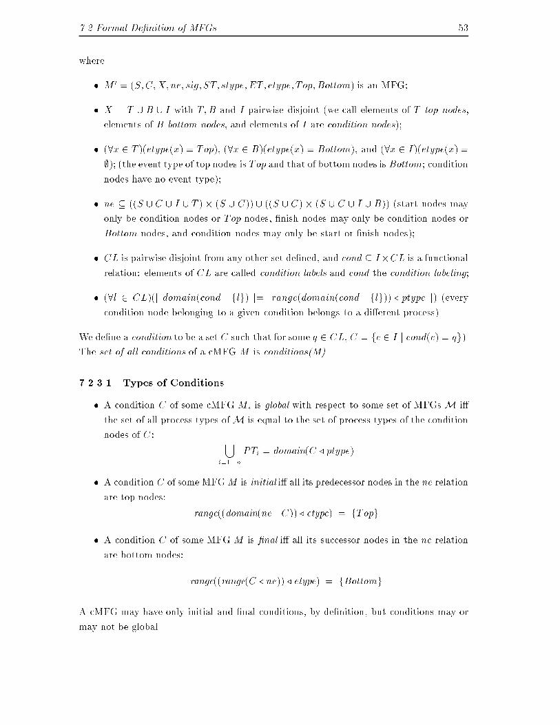
7.2 Formal De�nition of MFGs 53where� M 0 = (S;C;X;ne; sig; ST; stype; ET; etype; Top; Bottom) is an MFG;� X = T [ B [ I with T;B and I pairwise disjoint (we call elements of T top nodes,elements of B bottom nodes, and elements of I are condition nodes);� (8x 2 T )(etype(x) = Top), (8x 2 B)(etype(x) = Bottom), and (8x 2 I)(etype(x) =;); (the event type of top nodes is Top and that of bottom nodes is Bottom; conditionnodes have no event type);� ne � ((S [ C [ I [ T ) � (S [ C)) [ ((S [ C) � (S [ C [ I [ B)) (start nodes mayonly be condition nodes or Top nodes, �nish nodes may only be condition nodes orBottom nodes, and condition nodes may only be start or �nish nodes);� CL is pairwise disjoint from any other set de�ned, and cond � I�CL is a functionalrelation: elements of CL are called condition labels and cond the condition labeling;� (8l 2 CL)(j domain(cond . flg) j=j range(domain(cond . flg)) / ptype j) (everycondition node belonging to a given condition belongs to a di�erent process).We de�ne a condition to be a set C such that for some q 2 CL, C = fc 2 I j cond(c) = qg).The set of all conditions of a cMFG M is conditions(M).7.2.3.1 Types of Conditions� A condition C of some cMFG Ms is global with respect to some set of MFGs M i�the set of all process types ofM is equal to the set of process types of the conditionnodes of C: [i=1:::nPTi = domain(C / ptype)� A condition C of some MFGM is initial i� all its predecessor nodes in the ne relationare top nodes: range((domain(ne . C)) / etype) = fTopg� A condition C of some MFG M is �nal i� all its successor nodes in the ne relationare bottom nodes: range((range(C / ne)) / etype) = fBottomgA cMFG may have only initial and �nal conditions, by de�nition, but conditions may ormay not be global.

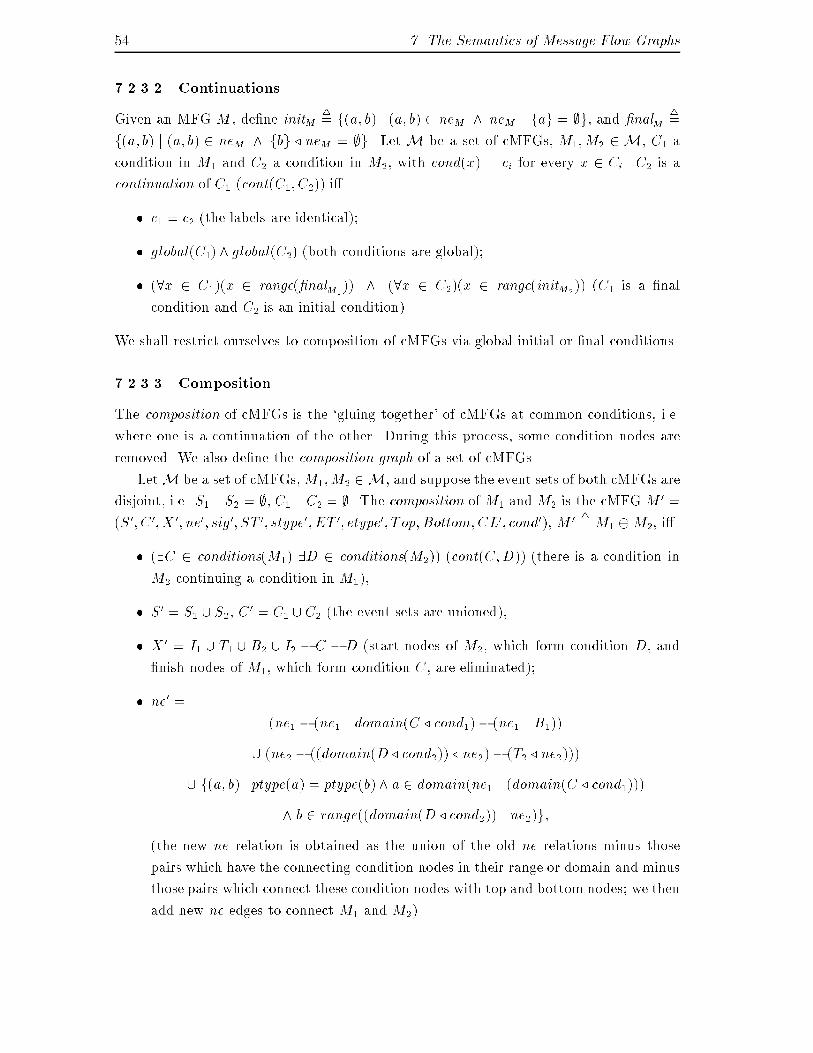
54 7. The Semantics of Message Flow Graphs7.2.3.2 ContinuationsGiven an MFG M , de�ne initM 4= f(a; b) j (a; b) 2 neM ^ neM . fag = ;g, and �nalM 4=f(a; b) j (a; b) 2 neM ^ fbg / neM = ;g. Let M be a set of cMFGs, M1;M2 2 M, C1 acondition in M1 and C2 a condition in M2, with cond(x) = ci for every x 2 Ci. C2 is acontinuation of C1 (cont(C1; C2)) i�� c1 = c2 (the labels are identical);� global(C1) ^ global(C2) (both conditions are global);� (8x 2 C1)(x 2 range(�nalM1)) ^ (8x 2 C2)(x 2 range(initM2)) (C1 is a �nalcondition and C2 is an initial condition).We shall restrict ourselves to composition of cMFGs via global initial or �nal conditions.7.2.3.3 CompositionThe composition of cMFGs is the `gluing together' of cMFGs at common conditions, i.e.where one is a continuation of the other. During this process, some condition nodes areremoved. We also de�ne the composition graph of a set of cMFGs.LetM be a set of cMFGs,M1;M2 2 M, and suppose the event sets of both cMFGs aredisjoint, i.e. S1 \S2 = ;, C1 \C2 = ;. The composition of M1 and M2 is the cMFGM 0 =(S0; C0; X 0; ne0; sig0; ST 0; stype0; ET 0; etype0; Top; Bottom;CL0; cond0), M 0 4=M1 �M2, i�� (9C 2 conditions(M1) 9D 2 conditions(M2)) (cont(C;D)) (there is a condition inM2 continuing a condition in M1),� S0 = S1 [ S2, C0 = C1 [ C2 (the event sets are unioned),� X 0 = I1 [ T1 [ B2 [ I2 � C � D (start nodes of M2, which form condition D, and�nish nodes of M1, which form condition C, are eliminated);� ne0 = (ne1 � (ne1 . domain(C / cond1)� (ne1 . B1))[ (ne2 � ((domain(D/ cond2)) / ne2)� (T2 / ne2)))[ f(a; b) j ptype(a) = ptype(b)^ a 2 domain(ne1 . (domain(C / cond1)))^ b 2 range((domain(D / cond2)) . ne2)g;(the new ne relation is obtained as the union of the old ne relations minus thosepairs which have the connecting condition nodes in their range or domain and minusthose pairs which connect these condition nodes with top and bottom nodes; we thenadd new ne edges to connect M1 and M2)

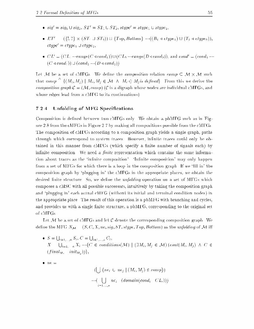
7.2 Formal De�nition of MFGs 55� sig0 = sig1 [ sig2, ST 0 = ST1 [ ST2, stype0 = stype1 [ stype2,� ET 0 = (f!; ?g � (ST1 [ ST2)) [ fTop; Bottomg � ((B1 / etype1) [ (T2 / etype2)),etype0 = etype1 [ etype2,� CL0 = (CL1� range(C / cond1))[ (CL2� range(D/cond2)), and cond0 = (cond1�(C / cond1)) [ (cond2 � (D / cond2)).Let M be a set of cMFGs. We de�ne the composition relation comp � M �M suchthat comp 4= f(Mi;Mj) j Mi;Mj 2 M ^ Mi �Mjis de�nedg. From this we derive thecomposition graph C = (M; comp) (C is a digraph whose nodes are individual cMFGs, andwhose edges lead from a cMFG to its continuations).7.2.4 Unfolding of MFG Speci�cationsComposition is de�ned between two cMFGs only. We obtain a pbMFG such as in Fig-ure 2.8 from the cMFGs in Figure 2.7 by making all compositions possible from the cMFGs.The composition of cMFGs according to a composition graph yields a single graph, pathsthrough which correspond to system traces. However, in�nite traces could only be ob-tained in this manner from cMFGs (which specify a �nite number of signals each) byin�nite composition. We need a �nite representation which contains the same informa-tion about traces as the `in�nite composition'. `In�nite composition' may only happenfrom a set of MFGs for which there is a loop in the composition graph. If we `�ll in' thecomposition graph by `plugging in' the cMFGs in the appropriate places, we obtain thedesired �nite structure. So, we de�ne the unfolding operation on a set of MFGs whichcomposes a cMSC with all possible successors, intuitively by taking the composition graphand `plugging in' each actual cMFG (without its initial and terminal condition nodes) inthe appropriate place. The result of this operation is a pbMFG with branching and cycles,and provides us with a single �nite structure, a pbMFG, corresponding to the original setof cMFGs.Let M be a set of cMFGs and let C denote the corresponding composition graph. Wede�ne the MFG NM = (S;C;X;ne; sig; ST; stype; Top;Bottom) as the unfolding ofM i�� S = Si=1;:::;n Si, C = Si=1;:::;nCi,X = Si=1;:::;nXi � fC 2 conditions(M) j (9Mi;Mj 2 M) (cont(Mi;Mj) ^ C 2(finalMi \ initMj ))g,� ne = ([ fnei [ nej j (Mi;Mj) 2 compg)� ( [i=1;:::;nnei . (domain(condi . CLi)))

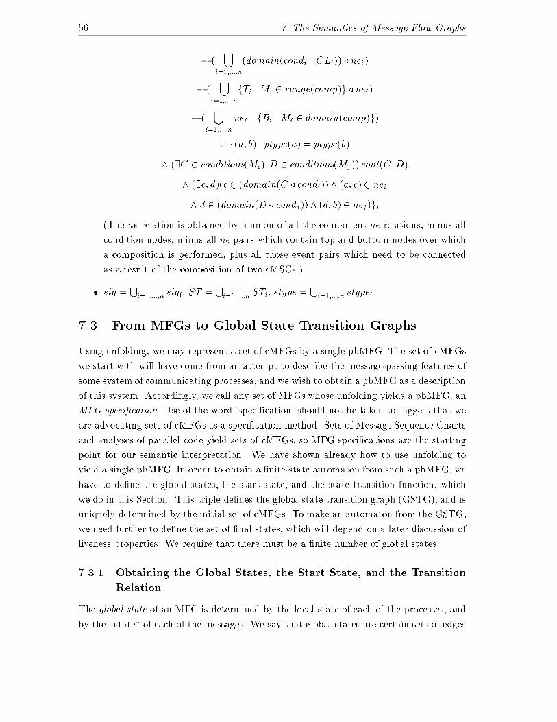
56 7. The Semantics of Message Flow Graphs� ( [i=1;:::;n(domain(condi . CLi)) / nei)� ( [i=1;:::;nfTi jMi 2 range(comp)g / nei)� ( [i=1;:::;nnei . fBi jMi 2 domain(comp)g)[ f(a; b) j ptype(a) = ptype(b)^ (9C 2 conditions(Mi); D 2 conditions(Mj)) cont(C;D)^ (9c; d)(c 2 (domain(C / condi))^ (a; c) 2 nei^ d 2 (domain(D / condj)) ^ (d; b) 2 nej)g;(The ne relation is obtained by a union of all the component ne relations, minus allcondition nodes, minus all ne pairs which contain top and bottom nodes over whicha composition is performed, plus all those event pairs which need to be connectedas a result of the composition of two cMSCs.)� sig = Si=1;:::;n sigi, ST = Si=1;:::;n STi, stype = Si=1;:::;n stypei.7.3 From MFGs to Global State Transition GraphsUsing unfolding, we may represent a set of cMFGs by a single pbMFG. The set of cMFGswe start with will have come from an attempt to describe the message-passing features ofsome system of communicating processes, and we wish to obtain a pbMFG as a descriptionof this system. Accordingly, we call any set of MFGs whose unfolding yields a pbMFG, anMFG speci�cation. Use of the word `speci�cation' should not be taken to suggest that weare advocating sets of cMFGs as a speci�cation method. Sets of Message Sequence Chartsand analyses of parallel code yield sets of cMFGs, so MFG speci�cations are the startingpoint for our semantic interpretation. We have shown already how to use unfolding toyield a single pbMFG. In order to obtain a �nite-state automaton from such a pbMFG, wehave to de�ne the global states, the start state, and the state transition function, whichwe do in this Section. This triple de�nes the global state transition graph (GSTG), and isuniquely determined by the initial set of cMFGs. To make an automaton from the GSTG,we need further to de�ne the set of �nal states, which will depend on a later discussion ofliveness properties. We require that there must be a �nite number of global states.7.3.1 Obtaining the Global States, the Start State, and the TransitionRelationThe global state of an MFG is determined by the local state of each of the processes, andby the \state" of each of the messages. We say that global states are certain sets of edges

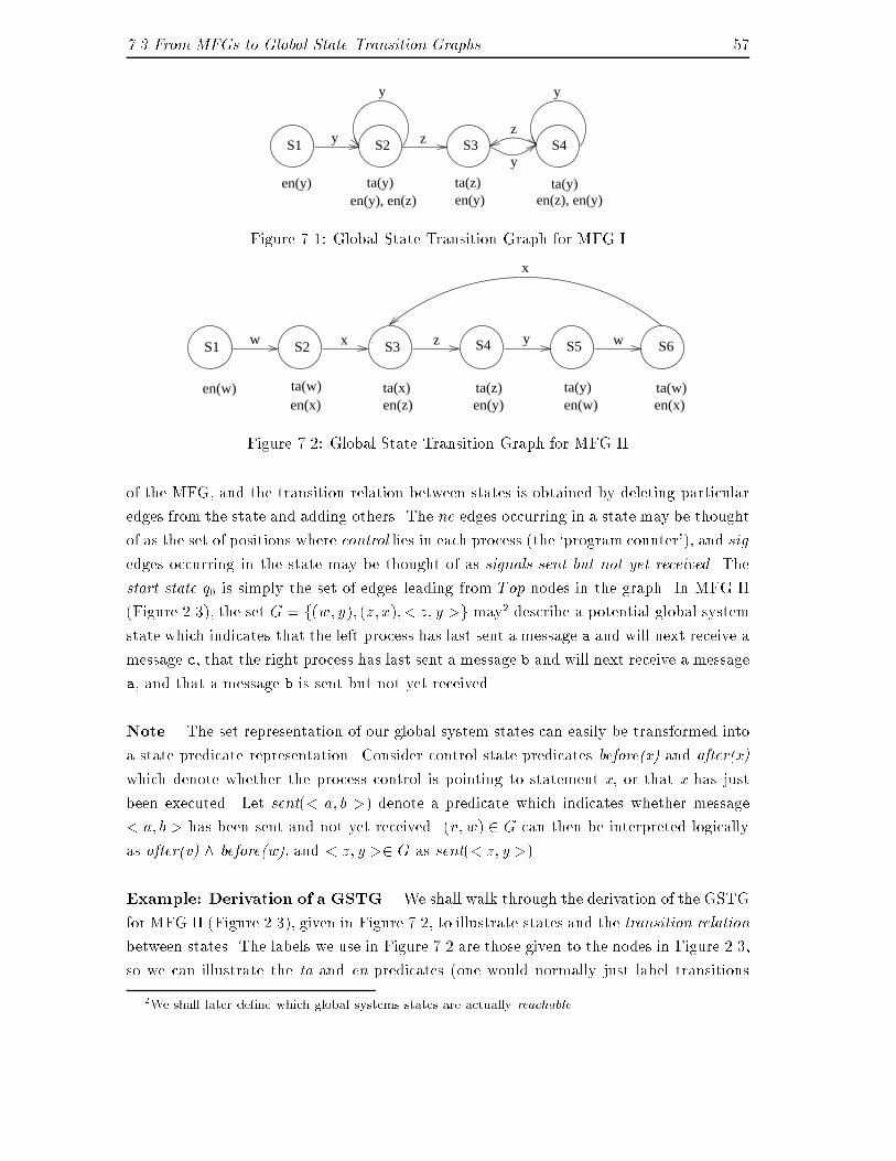
7.3 From MFGs to Global State Transition Graphs 57en(y)

S1 y

y

S2

ta(y)en(y), en(z)

ta(z)en(y)

S3z

y

y

ta(y)en(z), en(y)

S4zFigure 7.1: Global State Transition Graph for MFG IS1

en(w)

w

ta(w)en(x)

S2 x

ta(x)

S3 z S4

en(z)ta(z)en(y)

x

S5y w

en(w)ta(y)

en(x)ta(w)

S6Figure 7.2: Global State Transition Graph for MFG IIof the MFG, and the transition relation between states is obtained by deleting particularedges from the state and adding others. The ne edges occurring in a state may be thoughtof as the set of positions where control lies in each process (the `program counter'), and sigedges occurring in the state may be thought of as signals sent but not yet received. Thestart state q0 is simply the set of edges leading from Top nodes in the graph. In MFG II(Figure 2.3), the set G = f(w; y); (z; x);< z; y >g may2 describe a potential global systemstate which indicates that the left process has last sent a message a and will next receive amessage c, that the right process has last sent a message b and will next receive a messagea, and that a message b is sent but not yet received.Note. The set representation of our global system states can easily be transformed intoa state predicate representation. Consider control state predicates before(x) and after(x)which denote whether the process control is pointing to statement x, or that x has justbeen executed. Let sent(< a; b >) denote a predicate which indicates whether message< a; b > has been sent and not yet received. (v; w) 2 G can then be interpreted logicallyas after(v) ^ before(w), and < z; y >2 G as sent(< z; y >).Example: Derivation of a GSTG. We shall walk through the derivation of the GSTGfor MFG II (Figure 2.3), given in Figure 7.2, to illustrate states and the transition relationbetween states. The labels we use in Figure 7.2 are those given to the nodes in Figure 2.3,so we can illustrate the ta and en predicates (one would normally just label transitions2We shall later de�ne which global systems states are actually reachable.

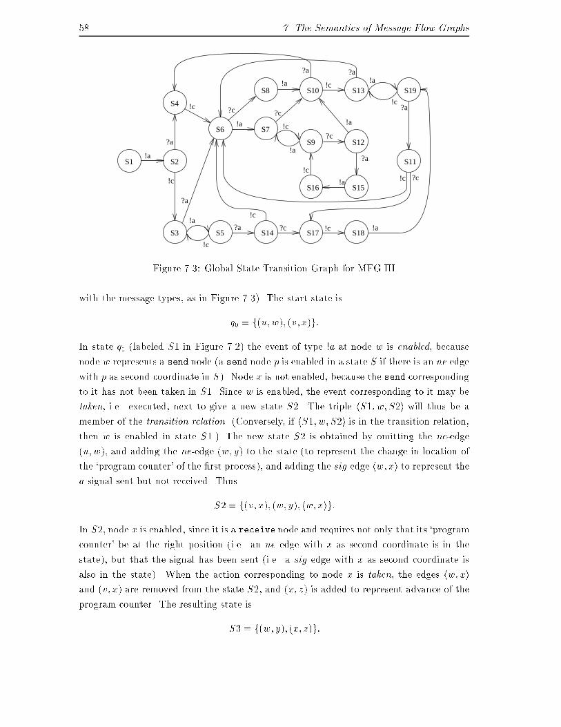
58 7. The Semantics of Message Flow GraphsS1 S2

S4

S3 S5

S6 S7

S9

S10

S12

S13 S19

S11

S15S16

S18S17S14

?a

!a !c

!a

?c

?a

!a

!c

!c

?a

!a?c !a

!a

!c

!c

?a

!c

!c

?c

!c

!a

?c

!c

?a

!a

!c ?c

S8!a

?a?a

Figure 7.3: Global State Transition Graph for MFG IIIwith the message types, as in Figure 7.3). The start state isq0 = f(u; w); (v; x)g:In state q0 (labeled S1 in Figure 7.2) the event of type !a at node w is enabled, becausenode w represents a send node (a send node p is enabled in a state S if there is an ne edgewith p as second coordinate in S). Node x is not enabled, because the send correspondingto it has not been taken in S1. Since w is enabled, the event corresponding to it may betaken, i.e. executed, next to give a new state S2. The triple hS1; w; S2i will thus be amember of the transition relation. (Conversely, if hS1; w; S2i is in the transition relation,then w is enabled in state S1.) The new state S2 is obtained by omitting the ne-edge(u; w), and adding the ne-edge (w; y) to the state (to represent the change in location ofthe `program counter' of the �rst process), and adding the sig edge hw; xi to represent thea signal sent but not received. ThusS2 = f(v; x); (w; y); hw; xig:In S2, node x is enabled, since it is a receive node and requires not only that its `programcounter' be at the right position (i.e. an ne edge with x as second coordinate is in thestate), but that the signal has been sent (i.e. a sig edge with x as second coordinate isalso in the state). When the action corresponding to node x is taken, the edges hw; xiand (v; x) are removed from the state S2, and (x; z) is added to represent advance of theprogram counter. The resulting state isS3 = f(w; y); (x; z)g:

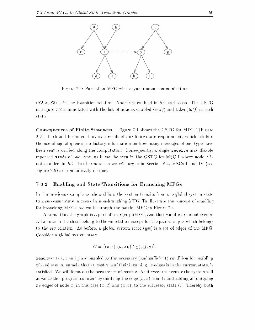
7.3 From MFGs to Global State Transition Graphs 59y

i

g

fb

x

a

c

d e hFigure 7.4: Part of an MFG with asynchronous communicationhS2; x; S3i is in the transition relation. Node z is enabled in S3, and so on. The GSTGin Figure 7.2 is annotated with the list of actions enabled (en()) and taken(ta()) in eachstate.Consequences of Finite-Stateness. Figure 7.1 shows the GSTG for MFG I (Figure2.2). It should be noted that as a result of our �nite-state requirement, which inhibitsthe use of signal queues, no history information on how many messages of one type havebeen sent is carried along the computation. Consequently, a single receive may disablerepeated sends of one type, as it can be seen in the GSTG for MSC I where node z isnot enabled in S3. Furthermore, as we will argue in Section 8.4, MSCs I and IV (seeFigure 2.5) are semantically distinct.7.3.2 Enabling and State Transitions for Branching MFGsIn the previous example we showed how the system transits from one global system stateto a successor state in case of a non-branching MFG. To illustrate the concept of enablingfor branching MFGs, we walk through the partial MFG in Figure 7.4.Assume that the graph is a part of a larger pbMFG, and that c and g are send events.All arrows in the chart belong to the ne relation except for the pair < x; y > which belongsto the sig relation. As before, a global system state (gss) is a set of edges of the MFG.Consider a global system stateG = f(a; c); (a; x); (f; y); (f; g)g:Send events c; x and g are enabled as the necessary (and su�cient) condition for enablingof send events, namely that at least one of their incoming ne-edges is in the current state, issatis�ed. We will focus on the occurrence of event x. As it executes event x the system willadvance the `program counter' by omitting the edge (a; x) from G and adding all outgoingne edges of node x, in this case (x; d) and (x; e), to the successor state G0. Thereby both

60 7. The Semantics of Message Flow Graphspotential successor events d and e are potentially enabled, depending only on whetherthey are send or receive events. However, one has to do a bit more, removing also thepossibility of choosing the enabled actions represented by c and g, which represent choicealternatives to the occurrence of the x event. Hence the edges (a; c) and (f; g) are removedfrom G as we transit via x to G0. Finally, one has to represent that the sending eventx leaves a message in transit, and thus the sig edge < x; y > is added to G to form thesuccessor state G0. HenceG0 = f(x; d); (x; e); < x; y >; (f; y); (f; g)g:We de�ne the transition relation formally in Section 7.4.7.3.3 GSTGs can be Complicated.It should be no surprise that GSTGs can rapidly become very complicated, for examplethe GSTG for MFG III in Figure 2.3 has nineteen states (Figure 7.3). This is partly dueto the asynchronous communication, and partly to interleavings of non-related events.MFG II and MFG III are similar, di�ering only in that the second message goes in op-posite directions. In MFG II this forces a unique execution sequence, and the GSTG iscorrespondingly simple (Figure 7.2). However, in MFG III, the two sends might occurbefore either receive, or alternatively sends and receives might be interleaved. Thusthe GSTG is more complex. However, it is not our intention to recommend explicit con-struction of the GSTG for every MFG, for the usual state-explosion reasons advancedin [74]. We use it later formally to relate liveness and safety properties as expressed intemporal logic or by B�uchi automata to MFGs.7.4 Formal De�nition of GSTGsThis Section provides the technical de�nition of Global State Transition Graphs, and maybe skipped on a �rst reading. We de�ne the notions of a global system state, of enablinga set of events in a global system state, and �nally the global state transition graph.7.4.1 EnablingA potential system state (pss) G � ne [ sig is any subset of the union of the ne and sigedges of the pbMFG. It is useful to de�ne state transitions for pss's. An (actual) globalsystem state (gss) will later be de�ned as a pss reached by taking the transitive closureof the transition relation from the start state (the set of all start nodes of the processes).De�nition of a gss therefore waits upon de�nition of the transition relation.Let V � S [ C denote a set of events and let G denote a potential system state. Wecall V enabled in G i� for every event in V one incoming ne edge is in G, and for every

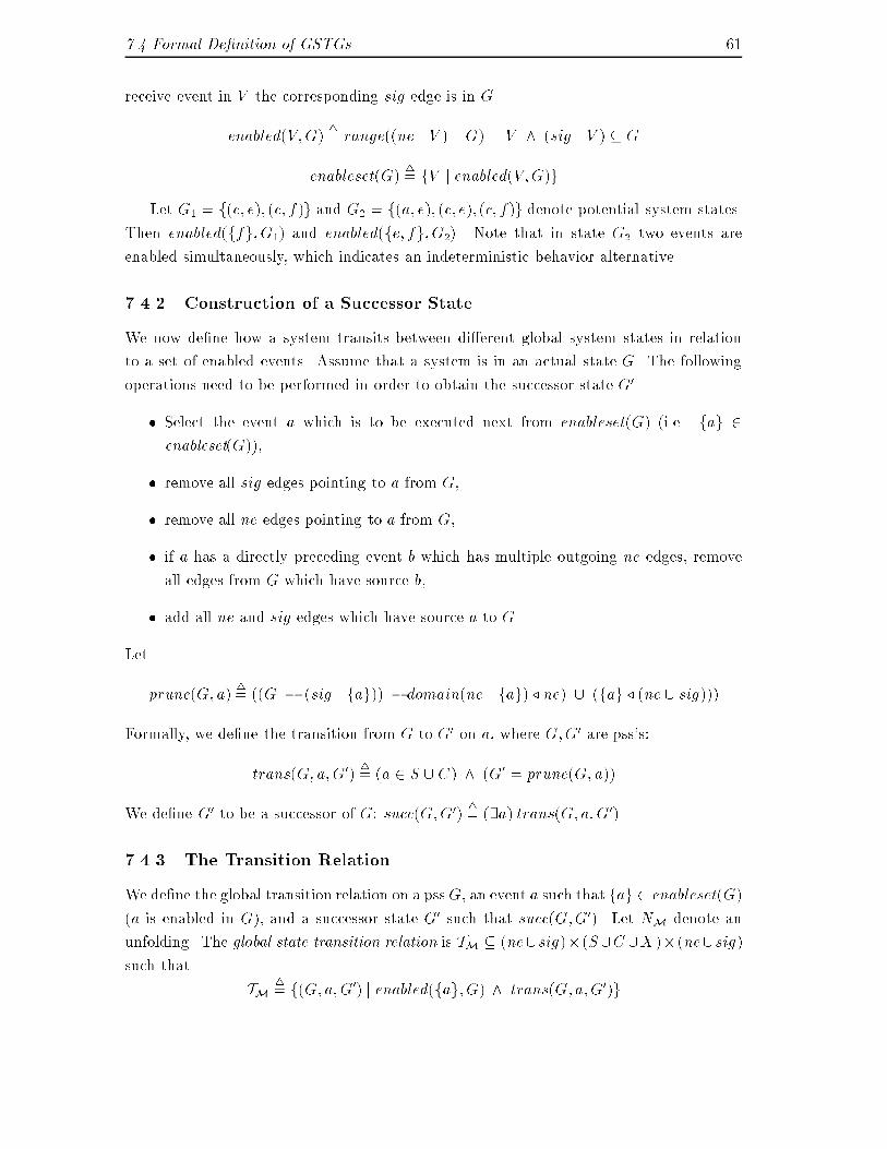
7.4 Formal De�nition of GSTGs 61receive event in V the corresponding sig edge is in G.enabled(V;G) 4= range((ne . V ) \ G) = V ^ (sig . V ) � Genableset(G) 4= fV j enabled(V;G)gLet G1 = f(c; e); (c; f)g and G2 = f(a; e); (c; e); (c; f)g denote potential system states.Then enabled(ffg; G1) and enabled(fe; fg; G2). Note that in state G2 two events areenabled simultaneously, which indicates an indeterministic behavior alternative.7.4.2 Construction of a Successor StateWe now de�ne how a system transits between di�erent global system states in relationto a set of enabled events. Assume that a system is in an actual state G. The followingoperations need to be performed in order to obtain the successor state G0.� Select the event a which is to be executed next from enableset(G) (i.e. fag 2enableset(G)),� remove all sig edges pointing to a from G,� remove all ne edges pointing to a from G,� if a has a directly preceding event b which has multiple outgoing ne edges, removeall edges from G which have source b,� add all ne and sig edges which have source a to G.Letprune(G; a) 4= ((G � (sig . fag)) � domain(ne . fag) / ne) [ (fag / (ne [ sig)))Formally, we de�ne the transition from G to G0 on a, where G;G0 are pss's:trans(G; a;G0) 4= (a 2 S [ C) ^ (G0 = prune(G; a))We de�ne G0 to be a successor of G: succ(G;G0) 4= (9a) trans(G; a;G0).7.4.3 The Transition RelationWe de�ne the global transition relation on a pssG, an event a such that fag 2 enableset(G)(a is enabled in G), and a successor state G0 such that succ(G;G0). Let NM denote anunfolding. The global state transition relation is TM � (ne[sig)� (S[C[X)� (ne[sig)such that TM 4= f(G; a;G0) j enabled(fag; G) ^ trans(G; a;G0)g

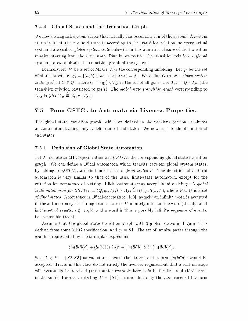
62 7. The Semantics of Message Flow Graphs7.4.4 Global States and the Transition Graph.We now distinguish system states that actually can occur in a run of the system. A systemstarts in its start state, and transits according to the transition relation, so every actualsystem state (called global system state below) is in the transitive closure of the transitionrelation starting from the start state. Finally, we restrict the transition relation to globalsystem states to obtain the transition graph of the system.Formally, letM be a set of MFGs, NM the corresponding unfolding. Let q0 be the setof start states, i.e. q0 = f(a; b) 2 ne j (fag / ne) = ;g. We de�ne G to be a global systemstate (gss) i� G 2 Q, where Q = fq0g / T +M is the set of all gss's. Let TM = Q / TM (thetransition relation restricted to gss's). The global state transition graph corresponding toNM is GSTGM 4= (Q; q0; TM).7.5 From GSTGs to Automata via Liveness PropertiesThe global state transition graph, which we de�ned in the previous Section, is almostan automaton, lacking only a de�nition of end-states. We now turn to the de�nition ofend-states.7.5.1 De�nition of Global State AutomatonLetM denote an MFG speci�cation and GSTGM the corresponding global state transitiongraph. We can de�ne a B�uchi automaton which transits between global system states,by adding to GSTGM a de�nition of a set of �nal states F . The de�nition of a B�uchiautomaton is very similar to that of the usual �nite-state automaton, except for thecriterion for acceptance of a string. B�uchi automata may accept in�nite strings. A globalstate automaton for GSTGM = (Q; q0; TM) is AM 4= (Q; q0; TM; F ), where F � Q is a setof �nal states. Acceptance is B�uchi-acceptance [143], namely an in�nite word is acceptedi� the automaton cycles through some state in F in�nitely often on the word (the alphabetis the set of events, e.g. ?a; !b, and a word is thus a possibly in�nite sequence of events,i.e. a possible trace).Assume that the global state transition graph with 3 global states in Figure 7.5 isderived from some MFG speci�cation, and q0 = S1. The set of in�nite paths through thegraph is represented by the !-regular expression(!a(!b?b)!) + (!a(!b?b)�?a)! + (!a(!b?b)�?a)�:(!a(!b?b)!):Selecting F = fS2; S3g as end-states means that traces of the form !a(!b?b)! would beaccepted. Traces in this class do not satisfy the liveness requirement that a sent messagewill eventually be received (the counter example here is !a in the �rst and third termsin the sum). However, selecting F = fS1g ensures that only the fair traces of the form

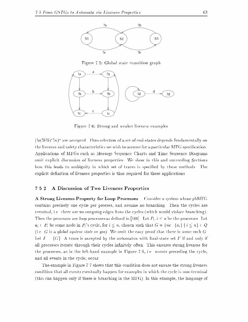
7.5 From GSTGs to Automata via Liveness Properties 63S1

?a

S2

?b

S3

!a !bFigure 7.5: Global state transition grapha

b d

c?c

!b

!a ?a

?b

!c

!d ?dFigure 7.6: Strong and weaker liveness examples(!a(!b?b)�?a)! are accepted. Thus selection of a set of end-states depends fundamentally onthe liveness and safety characteristics we wish to assume for a particular MFG speci�cation.Applications of MFGs such as Message Sequence Charts and Time Sequence Diagramsomit explicit discussion of liveness properties. We show in this and succeeding Sectionshow this leads to ambiguity in which set of traces is speci�ed by these methods. Theexplicit de�nition of liveness properties is thus required for these applications.7.5.2 A Discussion of Two Liveness PropertiesA Strong Liveness Property for Loop Processes. Consider a system whose pbMFGcontains precisely one cycle per process, and assume no branching. Then the cycles areterminal, i.e. there are no outgoing edges from the cycles (which would violate branching).Then the processes are loop processes as de�ned in [100]. Let Pi; i � n be the processes. Letai 2 Pi be some node in Pi's cycle, for i � n, chosen such that G = fne.faig j i � ng 2 Q(i.e. G is a global system state or gss). We omit the easy proof that there is some such G.Let F = fGg. A trace is accepted by the automaton with �nal-state set F if and only ifall processes iterate through their cycles in�nitely often. This ensures strong liveness forthe processes, as in the left-hand example in Figure 7.6, i.e. events preceding the cycle,and all events in the cycle, occur.The example in Figure 7.7 shows that this condition does not ensure the strong livenesscondition that all events eventually happen for examples in which the cycle is non-terminal(this can happen only if there is branching in the MFG). In this example, the language of

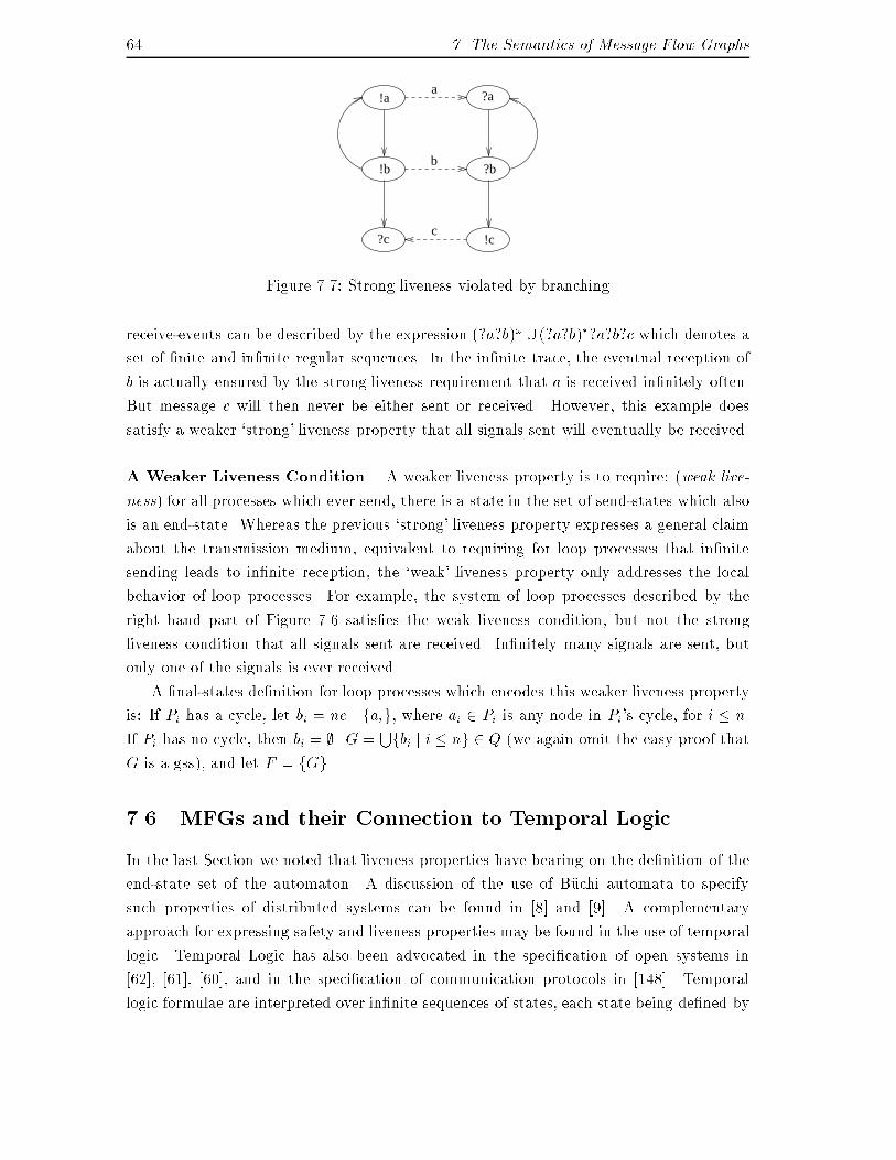
64 7. The Semantics of Message Flow Graphsa

b

c?c

!b

!a ?a

?b

!cFigure 7.7: Strong liveness violated by branchingreceive-events can be described by the expression (?a?b)! [ (?a?b)�?a?b?c which denotes aset of �nite and in�nite regular sequences. In the in�nite trace, the eventual reception ofb is actually ensured by the strong liveness requirement that a is received in�nitely often.But message c will then never be either sent or received. However, this example doessatisfy a weaker `strong' liveness property that all signals sent will eventually be received.A Weaker Liveness Condition. A weaker liveness property is to require: (weak live-ness) for all processes which ever send, there is a state in the set of send-states which alsois an end-state. Whereas the previous `strong' liveness property expresses a general claimabout the transmission medium, equivalent to requiring for loop processes that in�nitesending leads to in�nite reception, the `weak' liveness property only addresses the localbehavior of loop processes. For example, the system of loop processes described by theright hand part of Figure 7.6 satis�es the weak liveness condition, but not the strongliveness condition that all signals sent are received. In�nitely many signals are sent, butonly one of the signals is ever received.A �nal-states de�nition for loop processes which encodes this weaker liveness propertyis: If Pi has a cycle, let bi = ne . faig, where ai 2 Pi is any node in Pi's cycle, for i � n.If Pi has no cycle, then bi = ;. G = Sfbi j i � ng 2 Q (we again omit the easy proof thatG is a gss), and let F = fGg.7.6 MFGs and their Connection to Temporal LogicIn the last Section we noted that liveness properties have bearing on the de�nition of theend-state set of the automaton. A discussion of the use of B�uchi automata to specifysuch properties of distributed systems can be found in [8] and [9]. A complementaryapproach for expressing safety and liveness properties may be found in the use of temporallogic. Temporal Logic has also been advocated in the speci�cation of open systems in[62], [61], [60], and in the speci�cation of communication protocols in [148]. Temporallogic formulae are interpreted over in�nite sequences of states, each state being de�ned by

7.7 Formal De�nition of the Connection to Temporal Logic 65the truth values of state predicates. We relate these formulae to the automata obtainedfrom the semantics de�nition. We remain informal here, referring the reader to the formalde�nitions in Section 7.7 for more precision. We base our temporal logic interpretation onthe Manna-Pnueli approach [113].Basic Transition Systems. Following [113] we interpret global state transition graphsas so-called basic transition systems (BTS). A BTS consists of a �nite set of states �, atransition function � mapping a state to a set of possible successor states, and an initialcondition. We denote the set of all transitions � by T . For an MFG M , � will be the setof states Q of GSTGM , the transitions � will be the communication events that lead fromone global state to another, and the initial state of the BTS will be the initial state of theGSTG.Computations and State Predicates. Manna and Pnueli de�ne the following notions[113]. An in�nite state sequence � = s0; s1; : : : is a computation i� s0 is the initial state ofthe BTS, and for all consecutive pairs si; si+1 2 � there exists � 2 T such that si+1 2 �(si).The indices i of � are positions. Transition � is enabled at position i of some computation�, written as en(�), i� �(si) 6= ;. Transition � is (has been) taken at position i+1, writtenas ta(�), i� si+1 2 �(si).To correlate these de�nitions with the global state transition graph, we need to de�nethe enabled and taken predicates. Roughly speaking, a transition is enabled if it is enabledin the sense used earlier in Section 7.3. Similarly, a transition is taken in a state if thattransition has led to the state from an immediately preceding state (notice the `past tense'sense of the predicate taken).Temporal Logic. Given these interpretations of a GSTG as a model for temporal logic,we may de�ne a temporal logic in the usual way, e.g. [113]. The language has statepredicates en(�) and ta(�) as only basic propositions, includes the Boolean connectives (weuse just : and _ for simplicity), and the temporal operators3 (eventually), 2 (henceforth),3� (sometime in the past), � (previous) and S (since). The semantics is de�ned as usual.A temporal logic formula p is interpreted over state sequences �, and we de�ne the usualmodel-theoretic notion (�; i) j= p, that formula p is satis�ed in position i of sequence �.7.7 Formal De�nition of the Connection to Temporal LogicIn this Section, we formally de�ne the Manna-Pnueli-style temporal logic interpretationof GSTGs. The Section may be skipped on a �rst reading.Let NM = (S;C;X; ne; sig; ST; stype; Top; Bottom) denote the pbMFG unfolded fromsome MFG speci�cation M and let GSTGM = (Q; q0; TM) denote the corresponding

66 7. The Semantics of Message Flow GraphsGSTG. First, we relate the GSTG to a basic transition system as de�ned in [113]. Thenwe consider state predicates, computations and �nally the syntax and semantics of temporallogic.Basic Transition System. BTSM 4= (�;�; T ;�) is a basic transition system corre-sponding to GSTGM , where� � denotes a set of state variables, which is empty in the case of a set of cMFGs sincethey do not contain data3,� � denotes the �nite set of states, so � = Q.� T denotes a set of transitions, � : � ! 2�, for � 2 T . For s; s0 2 � let �(s) 4= fs0 j(s; �; s0) 2 TMg (the symbol � now has, harmlessly, both a GSTG syntax and a BTSsyntax). For MFGs, transitions are events of type !a or ?a, where a is a signal type.� � denotes an initial condition, in our case simply that the initial state is the initialstate q0 in GSTGM .The states of BTSM correspond to global system states of GSTGM (they are sets of edgesof the ne and sig relations), and the transitions � of BTSM correspond to communicationevents of the pbMFG obtained from the MFG speci�cation.State Predicates. Manna and Pnueli introduce an assertion which they call the transi-tion relation4 of the form �� : C�(�)^ (�y0 = �e) describing the change of the values of statevariables in state s to their values in state s0 into which the system transits from state sby taking transition � . Since � = ; for MFGs, C� is a constant, denoting the enablingcondition which describes the condition under which the state s may have a successorstate by taking the � transition. (�y0 = �e) stands for a conjunct which expresses the valuesof a sequence of state variables after the transition has been performed. Since there areno state variables in MFGs, this conjunct is vacuous, and so the transition relation �� isequivalent to the enabling condition C� (which is just that there is some � 0 2 �(s)) thus�� holds in a state s for some transition � i� there exists s0 2 � such that s0 2 �(s).Thus a transition � is enabled in some state s i� �(s) 6= ;. Conversely, � is disabled ins i� �(s) = ;. Mapping this to our MFG de�nitions we have that � is enabled in state s i�there is some state s0 such that hs; �; s0i 2 TM. Consequently, the Manna-Pnueli enablingcondition for an action � is true in precisely those GSTG states in which � is enabled inthe sense in which we de�ned this predicate for GSTGs earlier.3The only data in MFGs is signal type information, which is encoded in state information.4We will show that this notion is simpli�ed for MFGs, so there will be no confusion with our notion oftransition relation for GSTGs.

7.7 Formal De�nition of the Connection to Temporal Logic 67Computations and State Predicates en and ta. An in�nite state sequence � =s0; s1; : : : is a computation [113], i�� s0 j= �, which means just s0 = q0, and� for all consecutive pairs si; si+1 2 � there exists � 2 T such that si+1 2 �(si).The indices i of � are positions. Transition � is enabled (disabled) at position i of somecomputation � i� it is enabled (disabled) in si. We say that transition � is taken atposition i+ 1 i� si+1 2 �(si). We de�ne the predicate en(�) to hold in state si 2 � i� � isenabled at position i and we de�ne the predicate ta(�) to hold in state si 2 � i� � is takenat position i5. As noted, these de�nitions cohere with our former GSTG de�nitions. InFigures 7.2 and 7.1, we annotate each state with the instances of en and ta that are truein that state.Temporal Logic. We de�ne a temporal logic in the usual way, following [112]. Thelanguage has state predicates en(�) and ta(�) as basic propositions, includes the Booleanconnectives (we use just : and _ for simplicity), and the temporal operators 3 (eventu-ally), 2 (henceforth), 3� (sometime in the past), � (previous) and S (since).The semantics are de�ned as usual. A temporal logic formula p is interpreted overstate sequences �, and we de�ne (�; i) j= p, i.e. that formula p is satis�ed in position i ofsequence �.� If p is a basic assertion, then (�; i) j= p i� p is true in si as de�ned above.� (�; i) j= :p i� not (�; i) j= p� (�; i) j= p _ q i� (�; i) j= p or (�; i) j= q� (�; i) j= 3p i� for some j � i (�; j) j= p� (�; i) j= pSq i� for some k; 0 � k � i; (�; k) j= q,and for every j such that k < j � i; (�; j) j= p� (�; i) j= � p i� i > 0 and (�; i� 1) j= pAs syntactic abbreviations we introduce the following notation.� 2p 4= :3:p� 3�p 4= true S pWe say that a formula p holds on sequence � i� (�; 0) j= p, that it is satis�able i� it holdsfor some computation, and valid i� it holds for all computations.5In order to avoid notational confusion with our de�nitions for MFGs we distinguish our notationslightly from the notation used in [113].

68 7. The Semantics of Message Flow Graphs7.8 Logical Properties of MFGs.We can now give examples of properties expressed in temporal logic which can charac-terise pbMFGs obtained by unfolding sets of simple MFGs. In this Section, the MFGspeci�cations considered all contain simple cMFGs only. The classi�cation of propertiesas safety, recurrence, etc, refers to the classi�cation in [112].7.8.1 Properties Satis�ed by all MFG Speci�cationsThe following properties are satis�ed by all computations derived fromMFG speci�cations,as may be seen by inspection.1. Enabling of a send event (a safety property): If a send event is taken, it musthave been enabled previously. However, the enabling does not have to persist untilthe event is disabled, because a send event may also be disabled by a nondeterminis-tic behavior alternative (some branch is taken rather than another) in the process'scontrol ow. 2(ta(x) � 3�en(x))where x 2 S.2. Persistent enabling of a receive event: (a safety property) A receive eventmay only be taken if it has been previously enabled by a send event of the same type.Additionally, the enabling of a receive event can only be disabled by a receiveevent, therefore an enabling of a receive event persists up until the state when itis taken. 2(ta(y) � � (en(y) S ta(x)))where hx; yi 2 sig.7.8.2 Some Potential Requirements on MFG Speci�cations.Some liveness properties are not automatically ful�lled by an MFG speci�cationM . It wasnoted earlier that some of these properties were de�nable by making di�erent selectionsof the set of �nal states of a B�uchi automaton de�ned on GSTGM . If it is requiredfor an application that these properties should hold, they must explicitly be stated as anannotation to a pbMFG or an MFG speci�cation. Well-known examples of such propertiesare1. Weak fairness (a recurrence property): it is not the case that any transition �is enabled continuously without ever being taken.23(:en(�)_ ta(�))

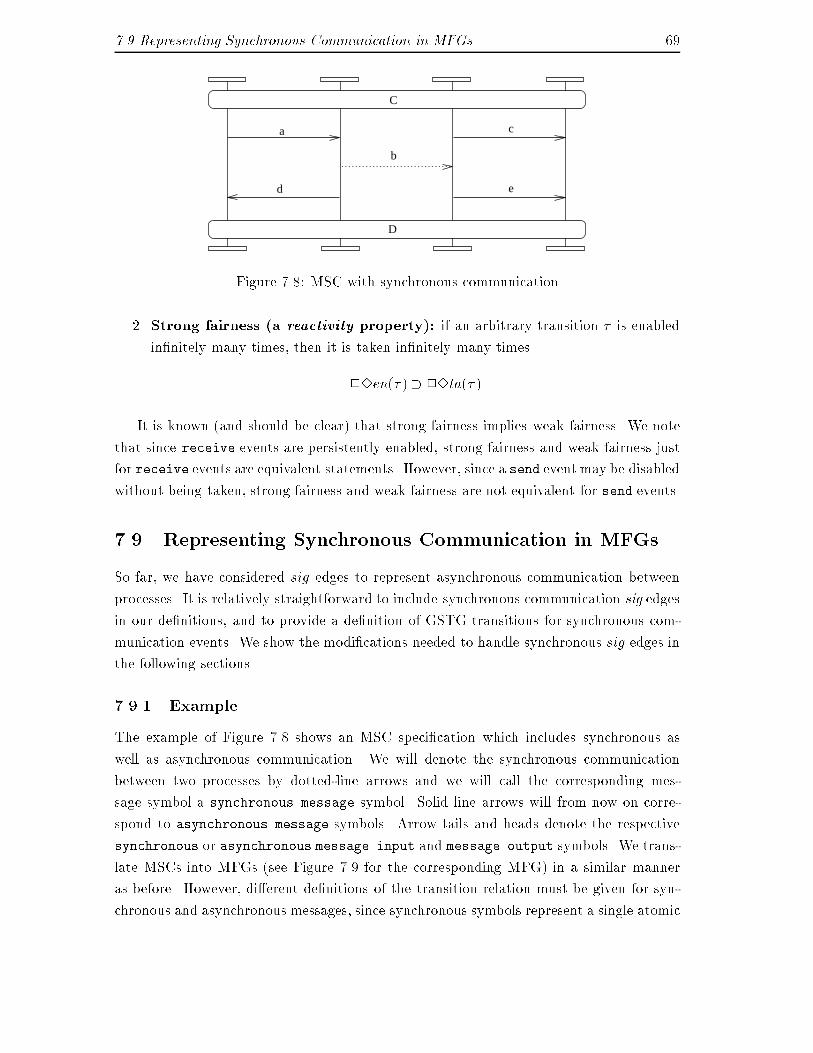
7.9 Representing Synchronous Communication in MFGs 69a

d

b

e

c

C

DFigure 7.8: MSC with synchronous communication2. Strong fairness (a reactivity property): if an arbitrary transition � is enabledin�nitely many times, then it is taken in�nitely many times.23en(�) � 23ta(�)It is known (and should be clear) that strong fairness implies weak fairness. We notethat since receive events are persistently enabled, strong fairness and weak fairness justfor receive events are equivalent statements. However, since a send event may be disabledwithout being taken, strong fairness and weak fairness are not equivalent for send events.7.9 Representing Synchronous Communication in MFGsSo far, we have considered sig edges to represent asynchronous communication betweenprocesses. It is relatively straightforward to include synchronous communication sig edgesin our de�nitions, and to provide a de�nition of GSTG transitions for synchronous com-munication events. We show the modi�cations needed to handle synchronous sig edges inthe following sections.7.9.1 ExampleThe example of Figure 7.8 shows an MSC speci�cation which includes synchronous aswell as asynchronous communication. We will denote the synchronous communicationbetween two processes by dotted-line arrows and we will call the corresponding mes-sage symbol a synchronous message symbol. Solid line arrows will from now on corre-spond to asynchronous message symbols. Arrow tails and heads denote the respectivesynchronous or asynchronous message input and message output symbols. We trans-late MSCs into MFGs (see Figure 7.9 for the corresponding MFG) in a similar manneras before. However, di�erent de�nitions of the transition relation must be given for syn-chronous and asynchronous messages, since synchronous symbols represent a single atomic

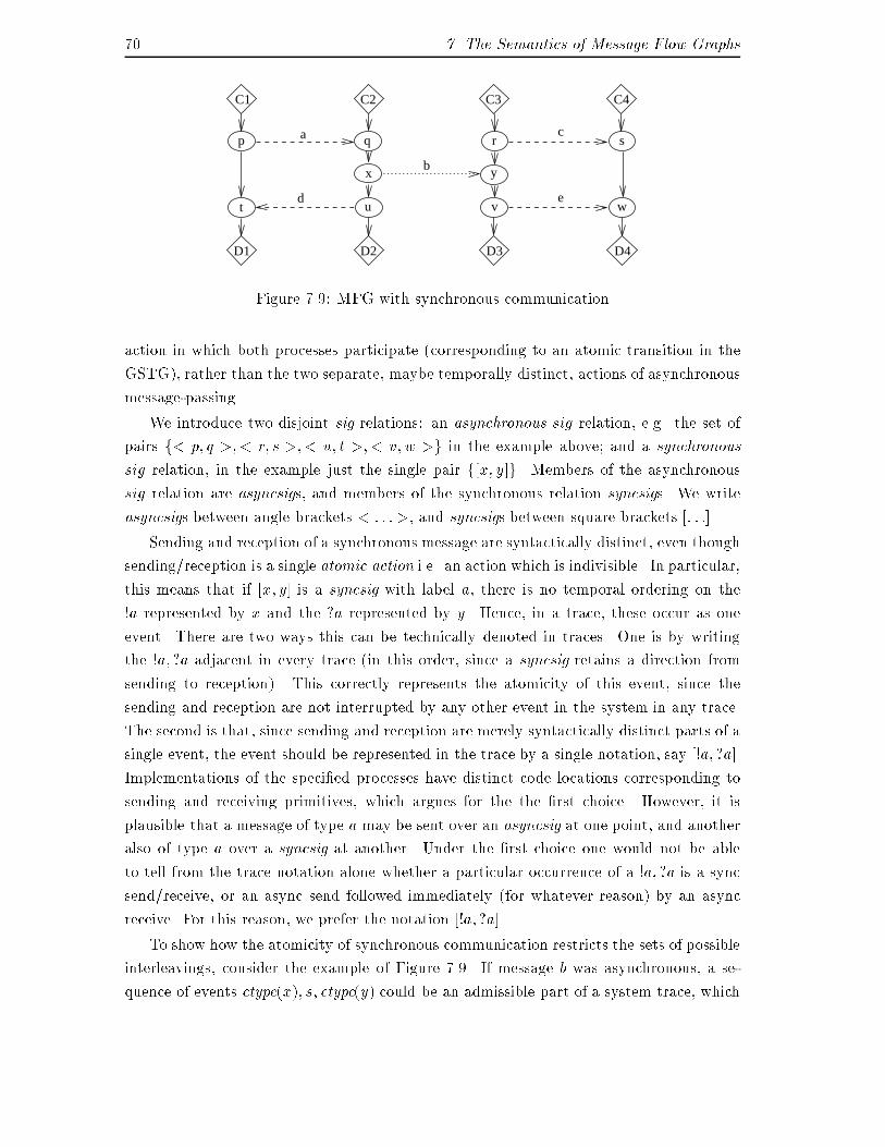
70 7. The Semantics of Message Flow Graphsa

d e

c

C1 C4

D2D1 D4

C3C2

p q

xb

r

y

ut v

D3

s

wFigure 7.9: MFG with synchronous communicationaction in which both processes participate (corresponding to an atomic transition in theGSTG), rather than the two separate, maybe temporally distinct, actions of asynchronousmessage-passing.We introduce two disjoint sig relations: an asynchronous sig relation, e.g. the set ofpairs f< p; q >;< r; s >;< u; t >;< v; w >g in the example above; and a synchronoussig relation, in the example just the single pair f[x; y]g. Members of the asynchronoussig relation are asyncsigs, and members of the synchronous relation syncsigs. We writeasyncsigs between angle brackets < : : : >, and syncsigs between square brackets [: : :].Sending and reception of a synchronous message are syntactically distinct, even thoughsending/reception is a single atomic action i.e. an action which is indivisible. In particular,this means that if [x; y] is a syncsig with label a, there is no temporal ordering on the!a represented by x and the ?a represented by y. Hence, in a trace, these occur as oneevent. There are two ways this can be technically denoted in traces. One is by writingthe !a; ?a adjacent in every trace (in this order, since a syncsig retains a direction fromsending to reception). This correctly represents the atomicity of this event, since thesending and reception are not interrupted by any other event in the system in any trace.The second is that, since sending and reception are merely syntactically distinct parts of asingle event, the event should be represented in the trace by a single notation, say [!a; ?a].Implementations of the speci�ed processes have distinct code locations corresponding tosending and receiving primitives, which argues for the the �rst choice. However, it isplausible that a message of type a may be sent over an asyncsig at one point, and anotheralso of type a over a syncsig at another. Under the �rst choice one would not be ableto tell from the trace notation alone whether a particular occurrence of a !a; ?a is a syncsend/receive, or an async send followed immediately (for whatever reason) by an asyncreceive. For this reason, we prefer the notation [!a; ?a].To show how the atomicity of synchronous communication restricts the sets of possibleinterleavings, consider the example of Figure 7.9. If message b was asynchronous, a se-quence of events etype(x); s; etype(y) could be an admissible part of a system trace, which

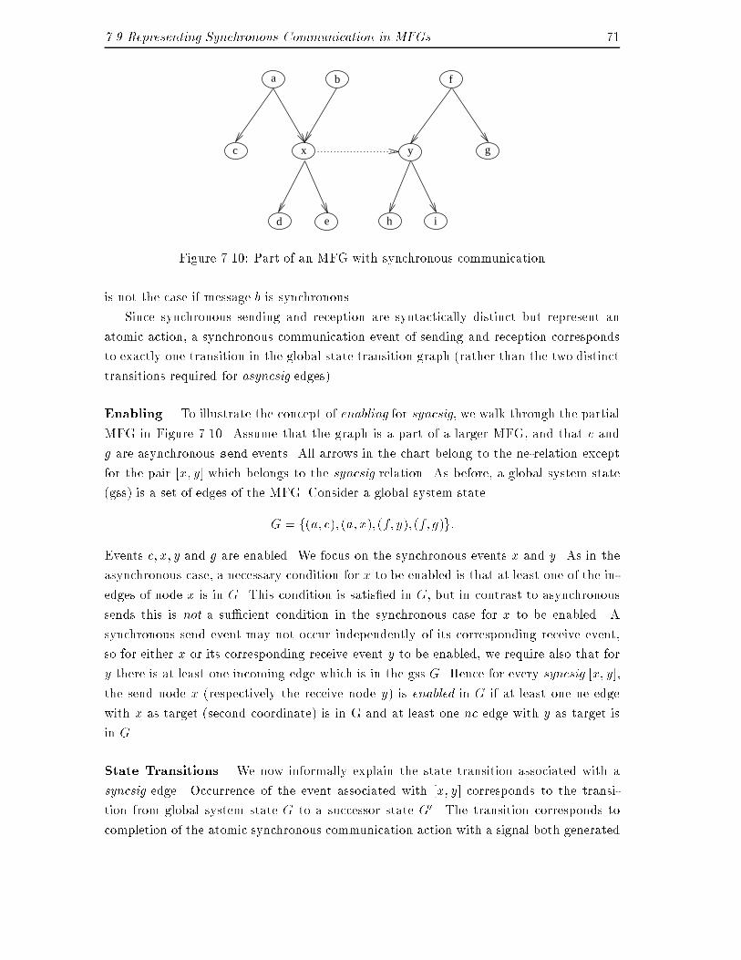
7.9 Representing Synchronous Communication in MFGs 71y

i

g

fb

x

a

c

d e hFigure 7.10: Part of an MFG with synchronous communicationis not the case if message b is synchronous.Since synchronous sending and reception are syntactically distinct but represent anatomic action, a synchronous communication event of sending and reception correspondsto exactly one transition in the global state transition graph (rather than the two distincttransitions required for asyncsig edges).Enabling. To illustrate the concept of enabling for syncsig, we walk through the partialMFG in Figure 7.10. Assume that the graph is a part of a larger MFG, and that c andg are asynchronous send events. All arrows in the chart belong to the ne-relation exceptfor the pair [x; y] which belongs to the syncsig relation. As before, a global system state(gss) is a set of edges of the MFG. Consider a global system stateG = f(a; c); (a; x); (f; y); (f; g)g:Events c; x; y and g are enabled. We focus on the synchronous events x and y. As in theasynchronous case, a necessary condition for x to be enabled is that at least one of the in-edges of node x is in G. This condition is satis�ed in G, but in contrast to asynchronoussends this is not a su�cient condition in the synchronous case for x to be enabled. Asynchronous send event may not occur independently of its corresponding receive event,so for either x or its corresponding receive event y to be enabled, we require also that fory there is at least one incoming edge which is in the gss G. Hence for every syncsig [x; y],the send node x (respectively the receive node y) is enabled in G if at least one ne edgewith x as target (second coordinate) is in G and at least one ne edge with y as target isin G.State Transitions. We now informally explain the state transition associated with asyncsig edge. Occurrence of the event associated with [x; y] corresponds to the transi-tion from global system state G to a successor state G0. The transition corresponds tocompletion of the atomic synchronous communication action with a signal both generated

72 7. The Semantics of Message Flow Graphsand received. This signal can never be `in transit' in any distinct system state, so it neverappears as part of a system state. Both nodes x and y are enabled in G, and the transitionoccurs as both processes advance their program counters to the next event, represented byomitting ne edges of the form (�; x) and (�; y) and adding edges of the form (x; �); (y; �)to the ne relation.As in the asynchronous case, however, one has to do a bit more, removing also thepossibility of choosing the enabled actions represented by c and g, which represent choicealternatives to the occurrence of the [x; y] event. Hence the edges (a; c) and (f; g) areremoved from G as we transit via [x; y] to G0. HenceG0 = f(x; d); (x; e); (y; h); (y; i)g:We de�ne the transition relation formally below.7.9.2 Formalisation of Extended Message Flow GraphsOur formal de�nitions are based on previous de�nitions. All parts of the de�nitions whichare not explicitly rede�ned here remain valid. We refer to MFGs with both synchronousand asynchronous communication as extended MFGs or XMFGs.Extended MFGs. To handle both asyncsigs and syncsigs, we simply split each set ofsend nodes (receive nodes) into two disjoint sets of syncsend (syncreceive) and asyncsend(asyncreceive) nodes, and the sig relation into two disjoint syncsig and asyncsig relations.Let Sa; Ss; Ca; Cs and X denote arbitrary pairwise disjoint sets, the elements of whichwe call asyncsend nodes, syncsend nodes, asyncrec nodes, syncrec nodes, and extra nodes.Let ST and ET denote arbitrary disjoint sets whose elements we call signal and eventtypes. For compatibility with the MFG de�nition we de�ne S 4= Sa[Ss, and C 4= Ca[Cs.An extended MFG is a tupleGX = (Sa; Ss; Ca; Cs; X; ne; siga; sigs; ST; stype; ET; etype; Top; Bottom)where (S[C[X; ne; etype; ET ) is a digraph with node labels, and (Sa[Ca; siga; stype; ST )and (Ss [ Cs; sigs; stype; ST ) are digraphs with edge labels satisfying the following condi-tions:1. siga � Sa � Ca2. sigs � Ss � Cs3. sig 4= siga [ sigs,4. all other conditions as for MFGs are satis�ed.This splitting of S, C and sig are the only changes required in the MFG (the `abstractsyntax'). Note that siga and sigc are both bipartite relations.

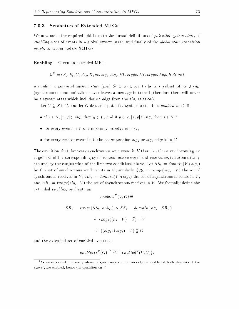
7.9 Representing Synchronous Communication in MFGs 737.9.3 Semantics of Extended MFGsWe now make the required additions to the formal de�nitions of potential system state, ofenabling a set of events in a global system state, and �nally of the global state transitiongraph, to accommodate XMFGs.Enabling. Given an extended MFGGX = (Sa; Ss; Ca; Cs; X; ne; siga; sigs; ST; stype; ET; etype; Top; Bottom)we de�ne a potential system state (pss) G � ne [ sig to be any subset of ne [ siga(synchronous communication never leaves a message in transit, therefore there will neverbe a system state which includes an edge from the sigs relation).Let V � S [ C, and let G denote a potential system state. V is enabled in G i�� if x 2 V; [x; y]2 sigs then y 2 V , and if y 2 V; [x; y] 2 sigs then x 2 V ,6� for every event in V one incoming ne edge is in G,� for every receive event in V the corresponding siga or sigs edge is in G.The condition that, for every synchronous send event in V there is at least one incoming needge in G of the corresponding synchronous receive event and vice versa, is automaticallyensured by the conjunction of the �rst two conditions above. Let SSV = domain(V /sigs)be the set of synchronous send events in V ; similarly SRV = range(sigs . V ) the set ofsynchronous receives in V ; ASV = domain(V / sigs) the set of asynchronous sends in V ;and ARV = range(sigs .V ) the set of asynchronous receives in V . We formally de�ne theextended enabling predicate as enabledX(V;G) 4=SRV = range(SSV / sigs) ^ SSV = domain(sigs . SRV )^ range((ne . V )\ G) = V^ ((sigs [ siga) . V ) � Gand the extended set of enabled events asenablesetX(G) 4= fV j enabledX(V;G)g:6As we explained informally above, a synchronous node can only be enabled if both elements of thesyncsig are enabled, hence the condition on V .

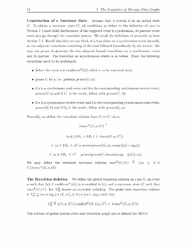
74 7. The Semantics of Message Flow GraphsConstruction of a Successor State. Assume that a system is in an actual stateG. To obtain a successor state G0, all conditions as before in the de�nition of succ inSection 7.4 must hold; furthermore, if the triggered event is synchronous, its partner eventmust also go through the transition process. We recall the de�nition of prune(G; a) fromSection 7.4. Recall also that we can think of a transition on a synchronous event formallyas two adjacent transitions consisting of the send followed immediately by the receive. Wemay use prune to generate the two adjacent formal transitions on a synchronous eventand its partner. The transition on asynchronous events is as before. Thus, the followingoperations need to be performed:� Select the event a 2 enablesetX(G) which is to be executed next;� prune G by a, i.e. perform prune(G; a);� if a is a synchronous send event and b is the corresponding synchronous receive event,prune(G; a) and if G1 is the result, follow with prune(G1; b);� if a is a synchronous receive event and b is the corresponding synchronous send event,prune(G; b) and if G2 is the result, follow with prune(G2; a).Formally, we de�ne the transition relation from G to G0 via a:transX (G; a;G0) 4=(a 2 (ASV [ARV ) ^ trans(G; a;G0))_ (a 2 SSV ^ G0 = prune(prune(G; a); range(fag / sigs)))_ (a 2 SRV ^ G0 = prune(prune(G; domain(sigs . fag)); a)):We may de�ne the extended successor relation succX(G;G0) 4= (9a 2 S [C) transX(G; a;G0).The Transition Relation. We de�ne the global transition relation on a pss G, an eventa such that fag 2 enablesetX(G) (a is enabled in G), and a successor state G0 such thatsuccX(G;G0). Let NXM denote an extended unfolding. The global state transition relationis T XM � (ne [ siga)� (S [ Ca [X)� (ne [ siga) such thatT XM 4= f(G; a;G0) j enabledX(G; fag; G0) ^ transX(G; a;G0)g:The notions of global system state and transition graph are as de�ned for MFGs.

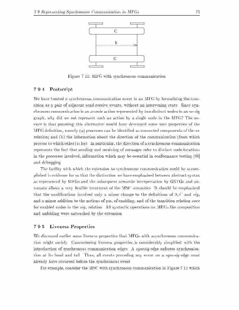
7.9 Representing Synchronous Communication in MFGs 75C

C

bFigure 7.11: MFG with synchronous communication7.9.4 PostscriptWe have treated a synchronous communication event in an MFG by formalising the tran-sition as a pair of adjacent send-receive events, without an intervening state. Since syn-chronous communication is an atomic action represented by two distinct nodes in an ne-siggraph, why did we not represent such an action by a single node in the MFG? The an-swer is that pursuing this alternative would have destroyed some nice properties of theMFG de�nition, namely (a) processes can be identi�ed as connected components of the nerelation; and (b) the information about the direction of the communication (from whichprocess to which other) is lost. In particular, the direction of a synchronous communicationrepresents the fact that sending and receiving of messages refer to distinct code-locationsin the processes involved, information which may be essential in conformance testing [80]and debugging.The facility with which the extension to synchronous communication could be accom-plished is evidence for us that the distinction we have emphasised between abstract syntaxas represented by MFGs and the subsequent semantic interpretation by GSTGs and au-tomata allows a very exible treatment of the MSC semantics. It should be emphasisedthat the modi�cations involved only a minor change to the de�nitions of S;C and sig,and a minor addition to the notions of pss, of enabling, and of the transition relation succfor enabled nodes in the sigs relation. All syntactic operations on MFGs like compositionand unfolding were untouched by the extension.7.9.5 Liveness PropertiesWe discussed earlier some liveness properties that MFGs with asynchronous communica-tion might satisfy. Guaranteeing liveness properties is considerably simpli�ed with theintroduction of synchronous communication edges. A syncsig edge enforces synchronisa-tion at its head and tail. Thus, all events preceding any event on a syncsig edge mustalready have occurred before the synchronous event.For example, consider the MSC with synchronous communication in Figure 7.11 which

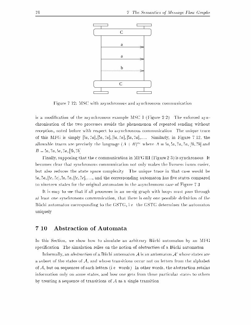
76 7. The Semantics of Message Flow GraphsC

a

C

a

bFigure 7.12: MSC with asynchronous and synchronous communicationis a modi�cation of the asynchronous example MSC I (Figure 2.2). The enforced syn-chronisation of the two processes avoids the phenomenon of repeated sending withoutreception, noted before with respect to asynchronous communication. The unique traceof this MFG is simply [!a; ?a]; [!a; ?a]; [!a; ?a]; [!a; ?a]; : : :. Similarly, in Figure 7.12, theallowable traces are precisely the language (A + B)1 where A = !a; !a; ?a; ?a; [!b; ?b] andB = !a; ?a; !a; ?a; [!b; ?b].Finally, supposing that the c communication in MFG III (Figure 2.3) is synchronous. Itbecomes clear that synchronous communication not only makes the liveness issues easier,but also reduces the state space complexity. The unique trace in that case would be!a; ?a; [!c; ?c]; !a; ?a; [!c; ?c]; : : :, and the corresponding automaton has �ve states comparedto nineteen states for the original automaton in the asynchronous case of Figure 7.3.It is easy to see that if all processes in an ne-sig graph with loops must pass throughat least one synchronous communication, that there is only one possible de�nition of theB�uchi automaton corresponding to the GSTG, i.e. the GSTG determines the automatonuniquely.7.10 Abstraction of AutomataIn this Section, we show how to simulate an arbitrary B�uchi automaton by an MFGspeci�cation. The simulation relies on the notion of abstraction of a B�uchi automaton.Informally, an abstraction of a B�uchi automatonA is an automatonA0 whose states area subset of the states of A, and whose transitions occur not on letters from the alphabetof A, but on sequences of such letters (i.e. words). In other words, the abstraction retainsinformation only on some states, and how one gets from these particular states to othersby treating a sequence of transitions of A as a single transition.

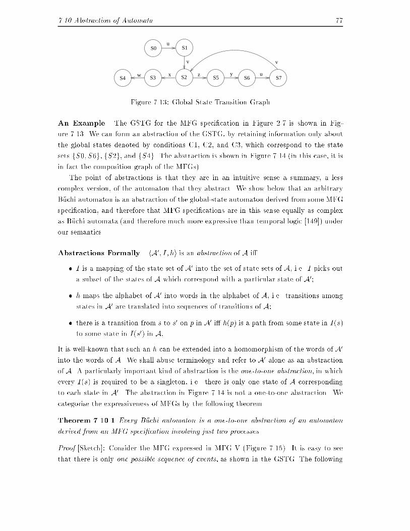
7.10 Abstraction of Automata 77u

S1

w x

v

z y u

v

S3

S0

S4 S2 S5 S6 S7Figure 7.13: Global State Transition GraphAn Example. The GSTG for the MFG speci�cation in Figure 2.7 is shown in Fig-ure 7.13. We can form an abstraction of the GSTG, by retaining information only aboutthe global states denoted by conditions C1, C2, and C3, which correspond to the statesets fS0; S6g, fS2g, and fS4g. The abstraction is shown in Figure 7.14 (in this case, it isin fact the composition graph of the MFGs).The point of abstractions is that they are in an intuitive sense a summary, a lesscomplex version, of the automaton that they abstract. We show below that an arbitraryB�uchi automaton is an abstraction of the global-state automaton derived from some MFGspeci�cation, and therefore that MFG speci�cations are in this sense equally as complexas B�uchi automata (and therefore much more expressive than temporal logic [149]) underour semantics.Abstractions Formally. hA0; I; hi is an abstraction of A i�� I is a mapping of the state set of A0 into the set of state sets of A, i.e. I picks outa subset of the states of A which correspond with a particular state of A0;� h maps the alphabet of A0 into words in the alphabet of A, i.e. transitions amongstates in A0 are translated into sequences of transitions of A;� there is a transition from s to s0 on p in A0 i� h(p) is a path from some state in I(s)to some state in I(s0) in A,It is well-known that such an h can be extended into a homomorphism of the words of A0into the words of A. We shall abuse terminology and refer to A0 alone as an abstractionof A. A particularly important kind of abstraction is the one-to-one abstraction, in whichevery I(s) is required to be a singleton, i.e. there is only one state of A correspondingto each state in A0. The abstraction in Figure 7.14 is not a one-to-one abstraction. Wecategorise the expressiveness of MFGs by the following theorem.Theorem 7.10.1 Every B�uchi automaton is a one-to-one abstraction of an automatonderived from an MFG speci�cation involving just two processes.Proof [Sketch]: Consider the MFG expressed in MFG V (Figure 7.15). It is easy to seethat there is only one possible sequence of events, as shown in the GSTG. The following

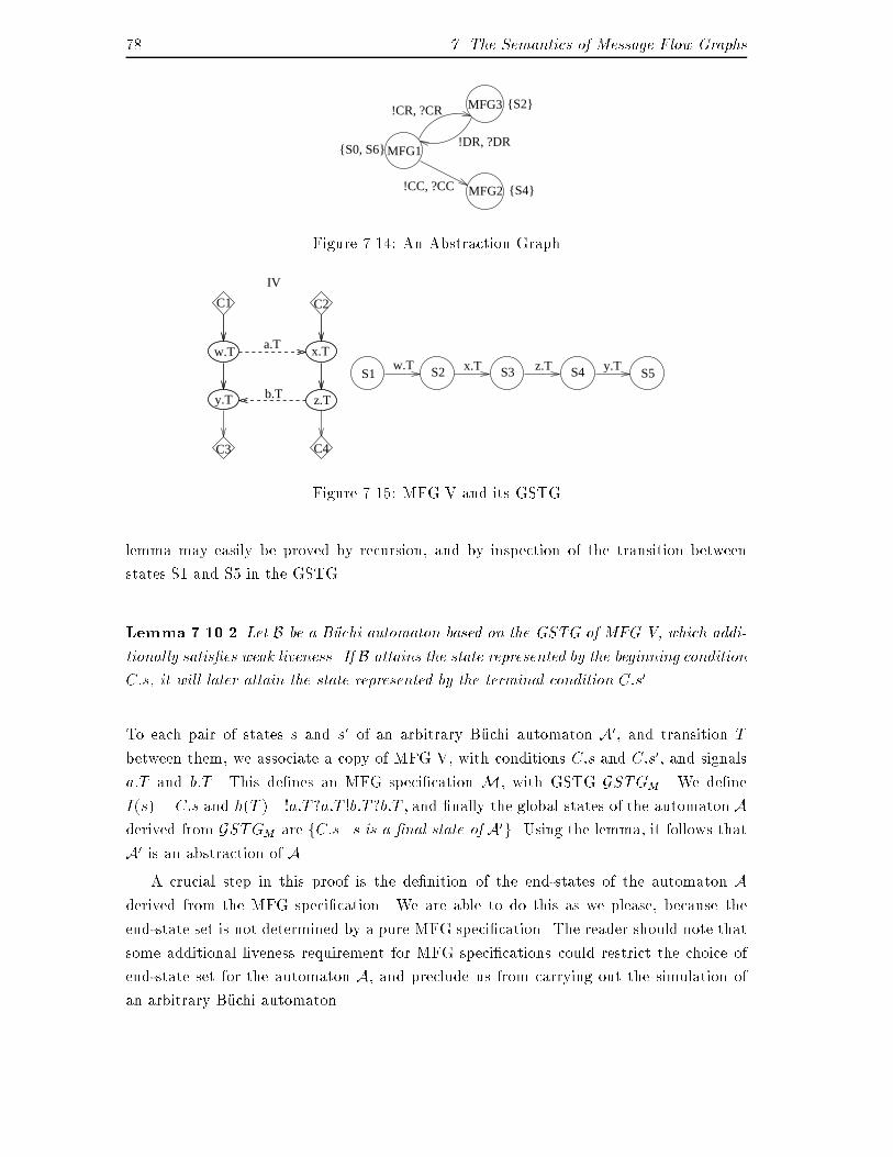
78 7. The Semantics of Message Flow GraphsMFG1

MFG2

MFG3!CR, ?CR

!DR, ?DR

!CC, ?CC

{S0, S6}

{S4}

{S2}Figure 7.14: An Abstraction Grapha.T

b.T

w.T x.T z.T y.T

C1 C2

w.T x.T

y.T z.T

C3 C4

S1 S2 S3 S4 S5

IV

Figure 7.15: MFG V and its GSTGlemma may easily be proved by recursion, and by inspection of the transition betweenstates S1 and S5 in the GSTG.Lemma 7.10.2 Let B be a B�uchi automaton based on the GSTG of MFG V, which addi-tionally satis�es weak liveness. If B attains the state represented by the beginning conditionC:s, it will later attain the state represented by the terminal condition C:s0.To each pair of states s and s0 of an arbitrary B�uchi automaton A0, and transition Tbetween them, we associate a copy of MFG V, with conditions C:s and C:s0, and signalsa:T and b:T . This de�nes an MFG speci�cation M, with GSTG GSTGM . We de�neI(s) = C:s and h(T ) =!a:T?a:T !b:T?b:T , and �nally the global states of the automaton Aderived from GSTGM are fC:s j s is a �nal state of A0g. Using the lemma, it follows thatA0 is an abstraction of A.A crucial step in this proof is the de�nition of the end-states of the automaton Aderived from the MFG speci�cation. We are able to do this as we please, because theend-state set is not determined by a pure MFG speci�cation. The reader should note thatsome additional liveness requirement for MFG speci�cations could restrict the choice ofend-state set for the automaton A, and preclude us from carrying out the simulation ofan arbitrary B�uchi automaton.

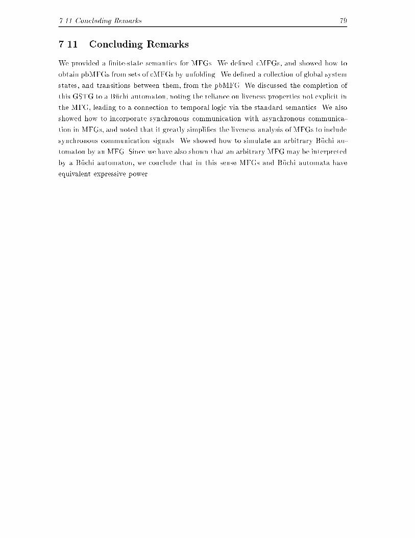
7.11 Concluding Remarks 797.11 Concluding RemarksWe provided a �nite-state semantics for MFGs. We de�ned cMFGs, and showed how toobtain pbMFGs from sets of cMFGs by unfolding. We de�ned a collection of global systemstates, and transitions between them, from the pbMFG. We discussed the completion ofthis GSTG to a B�uchi automaton, noting the reliance on liveness properties not explicit inthe MFG, leading to a connection to temporal logic via the standard semantics. We alsoshowed how to incorporate synchronous communication with asynchronous communica-tion in MFGs, and noted that it greatly simpli�es the liveness analysis of MFGs to includesynchronous communication signals. We showed how to simulate an arbitrary B�uchi au-tomaton by an MFG. Since we have also shown that an arbitrary MFG may be interpretedby a B�uchi automaton, we conclude that in this sense MFGs and B�uchi automata haveequivalent expressive power.

Chapter 8Discussion of Some Issues in theSemanticsWe now discuss a few more issues arising from our semantics. We required that a systemdescribed by an MFG has global states with respect to its message-passing behavior, withinstantaneous transitions between these states e�ected by atomic message-passing actions.Under this assumption, we argue now that� the unrestricted use of `conditions' requires processes to keep control history variablesof unbounded size,� that allowing `crossing' messages of the same type implies certain properties of theenvironment that are neither explicit nor desirable,� that MFG speci�cations can `count' receptions of messages, and� that liveness properties of MFGs are more easily expressed by temporal logic formulasover the control states than by B�uchi acceptance conditions over the same set ofstates.8.1 IntroductionThe purpose of this Chapter is to discuss issues arising from the task of giving a precisemathematical semantics for MFGs and MSCs. Seemingly innocuous syntactic choices,made for example in the syntactic de�nition of MSCs in Z.120, may have profound andsomewhat contrary semantic consequences. We point out some of those consequences here,not to resolve them (for resolution depends on standardisation group consensus), but toemphasise both the need for resolution, and the danger of introducing syntactic featureswithout thinking through their semantic consequences.

82 8. Discussion of Some Issues in the SemanticsIt is generally accepted that the underlying ontology of MFGs (e.g. in their MSC form)is that of events (as also in the various proposed MSC semantics of [134, 48, 64]). We cansummarise the representation of event features in an MFG as follows:� (a) represented events are message sends and receives only;� (b) the occurrence of an event is represented;� (c) the order of occurrence of events within an individual process is represented;� (d) the types of the events are represented.These features are represented in the message-passing fragments of other imperative lan-guages such as the original version of CSP [70], Esterel [23], Estelle [49] or SDL [32].Representing this information in a graph such as an MFG is a mathematically more pre-cise reformulation of the pictorial information about events and their ordering. However,this is not all the information that an MFG appears to contain. It is an additional featureof MFGs, not present in either CSP, Esterel, Estelle or SDL, that each of these events (in asimple MFG) or `program statements' (in MFGs with conditions) is somehow `connected'to precisely one other,1 (c.f. the property (*) for MFGs in Section 2.4). A semantics ofMFGs must explain how and what this connection is supposed to denote.Next we brie y describe the issues concerning the semantics of MFGs discussed in theremainder of this Chapter.The problem of non-local choice. Because of the requirements of the MSC standard,in order to treat MSCs as MFGs we de�ned a notion of condition for MFGs, and com-position of MFGs by conditions (see Section 7.2.3.3). Conditions are global labels suchthat two MFGs may be `joined' at this label. By allowing more than one possible joining,one obtains the e�ect of non-deterministic choice in MFGs (but conditionals de�ned onthe values of state predicates are still not possible). By writing the same condition atthe beginning as well as the end of an MFG, one obtains non-terminating-loop-like be-havior. We argue in Section 8.2 that the unimpeded use of conditions requires the use ofunbounded history variables ranging over decision predicates in order to resolve non-localchoices. In other words, a complete history of control branching must be accessible to aprocess, and must either be held by the environment, and communicated implicitly to aprocess on demand, or must be communicated implicitly by the environment to a processdynamically, and held in a history variable of potentially unbounded size in the processitself.1This may not quite be accurate. MSCs used informally sometimes have sends going nowhere, toindicate a lost message. But this is not in the MSC standard, and we do not think it's particularlysigni�cant for the argument made here.

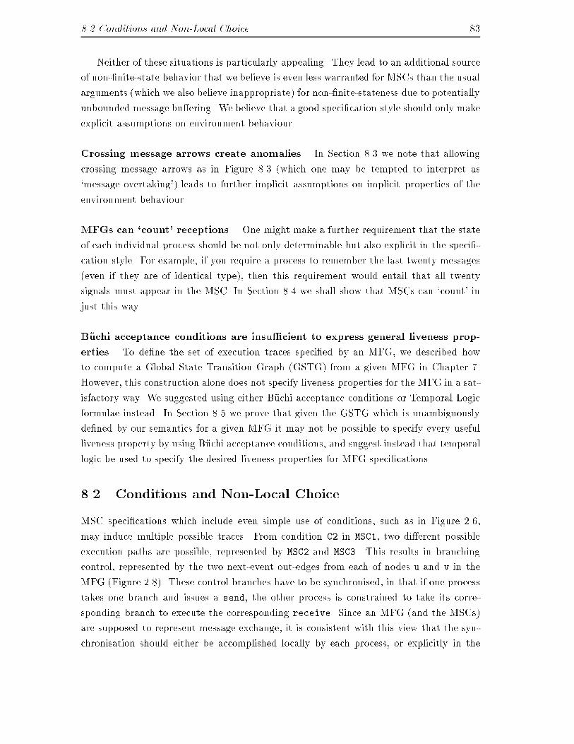
8.2 Conditions and Non-Local Choice 83Neither of these situations is particularly appealing. They lead to an additional sourceof non-�nite-state behavior that we believe is even less warranted for MSCs than the usualarguments (which we also believe inappropriate) for non-�nite-stateness due to potentiallyunbounded message bu�ering. We believe that a good speci�cation style should only makeexplicit assumptions on environment behaviour.Crossing message arrows create anomalies. In Section 8.3 we note that allowingcrossing message arrows as in Figure 8.3 (which one may be tempted to interpret as`message overtaking') leads to further implicit assumptions on implicit properties of theenvironment behaviour.MFGs can `count' receptions. One might make a further requirement that the stateof each individual process should be not only determinable but also explicit in the speci�-cation style. For example, if you require a process to remember the last twenty messages(even if they are of identical type), then this requirement would entail that all twentysignals must appear in the MSC. In Section 8.4 we shall show that MSCs can `count' injust this way.B�uchi acceptance conditions are insu�cient to express general liveness prop-erties. To de�ne the set of execution traces speci�ed by an MFG, we described howto compute a Global State Transition Graph (GSTG) from a given MFG in Chapter 7.However, this construction alone does not specify liveness properties for the MFG in a sat-isfactory way. We suggested using either B�uchi acceptance conditions or Temporal Logicformulae instead. In Section 8.5 we prove that given the GSTG which is unambiguouslyde�ned by our semantics for a given MFG it may not be possible to specify every usefulliveness property by using B�uchi acceptance conditions, and suggest instead that temporallogic be used to specify the desired liveness properties for MFG speci�cations.8.2 Conditions and Non-Local ChoiceMSC speci�cations which include even simple use of conditions, such as in Figure 2.6,may induce multiple possible traces. From condition C2 in MSC1, two di�erent possibleexecution paths are possible, represented by MSC2 and MSC3. This results in branchingcontrol, represented by the two next-event out-edges from each of nodes u and v in theMFG (Figure 2.8). These control branches have to be synchronised, in that if one processtakes one branch and issues a send, the other process is constrained to take its corre-sponding branch to execute the corresponding receive. Since an MFG (and the MSCs)are supposed to represent message exchange, it is consistent with this view that the syn-chronisation should either be accomplished locally by each process, or explicitly in the

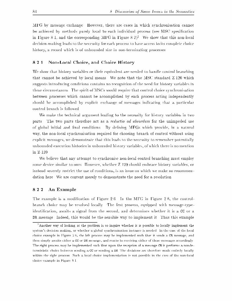
84 8. Discussion of Some Issues in the SemanticsMFG by message exchange. However, there are cases in which synchronisation cannotbe achieved by methods purely local to each individual process (see MSC speci�cationin Figure 8.1, and the corresponding MFG in Figure 8.2)2. We show that this non-localdecision-making leads to the necessity for each process to have access to its complete choicehistory, a record which is of unbounded size in non-terminating processes.8.2.1 Non-Local Choice, and Choice HistoryWe show that history variables or their equivalent are needed to handle control branchingthat cannot be achieved by local means. We note that the MSC standard Z.120 whichsuggests introducing conditions contains no recognition of the need for history variables inthese circumstances. The spirit of MSCs would require that control choice synchronisationbetween processes which cannot be accomplished by each process acting independentlyshould be accomplished by explicit exchange of messages indicating that a particularcontrol branch is followed.We make the technical argument leading to the necessity for history variables in twoparts. The two parts therefore act as a reductio ad absurdum for the unimpeded useof global initial and �nal conditions. By de�ning MFGs which provide, in a naturalway, the non-local synchronisation required for choosing branch of control without usingexplicit messages, we demonstrate that this leads to the necessity to remember potentiallyunbounded execution histories in unbounded history variables, of which there is no mentionin Z.120.We believe that any attempt to synchronise non-local control branching must employsome device similar to ours. However, whether Z.120 should embrace history variables, orinstead severely restrict the use of conditions, is an issue on which we make no recommen-dation here. We are content merely to demonstrate the need for a resolution.8.2.2 An ExampleThe example is a modi�cation of Figure 2.6. In the MFG in Figure 2.8, the control-branch choice may be resolved locally. The �rst process, equipped with message-type-identi�cation, awaits a signal from the second, and determines whether it is a CC or aDR message. Indeed, this would be the sensible way to implement it. Thus this example2Another way of looking at the problem is to inquire whether it is possible to locally implement thesystem's decision making, or whether a global synchronization instance is needed. In the case of the localchoice example in Figure 2.6, the left process may be implemented such that it sends a CR message, andthen simply awaits either a CC or DR message, and reacts to receiving either of these messages accordingly.The right process may be implemented such that upon the reception of a message CR it performs a nonde-terministic choice between sending a CC or sending a DR. The decisions are therefore made entirely locallywithin the right process. Such a local choice implementation is not possible in the case of the non-localchoice example in Figure 8.1.

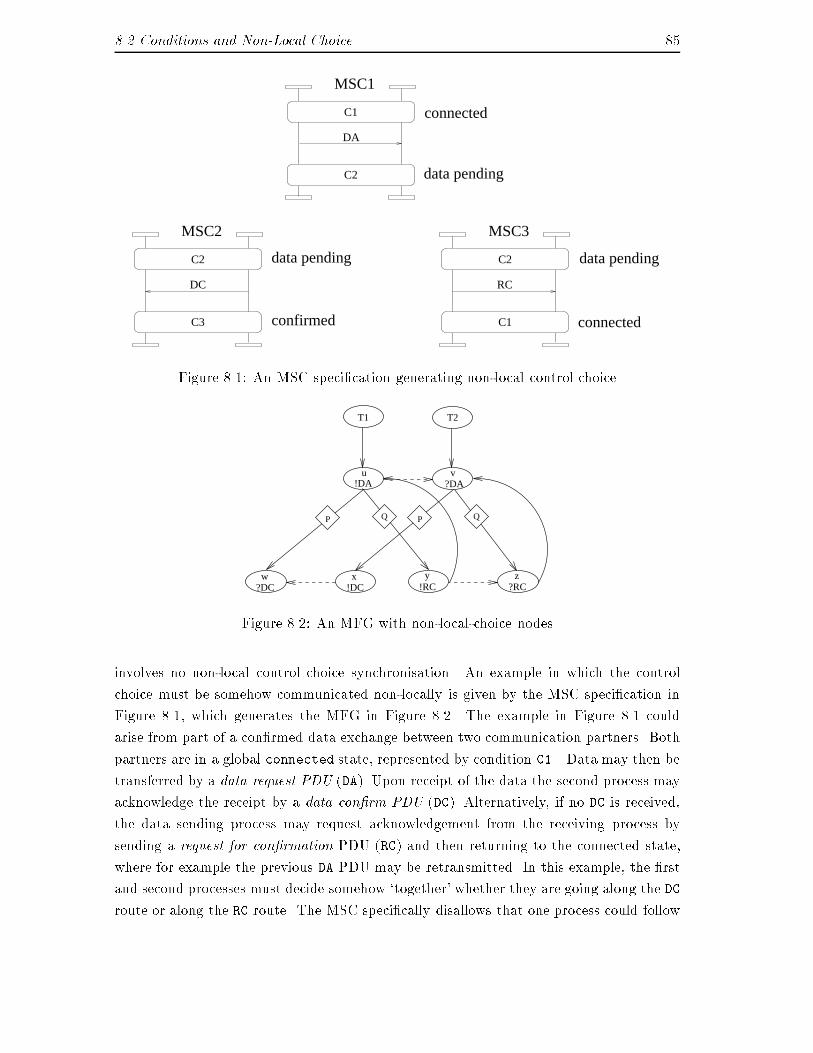
8.2 Conditions and Non-Local Choice 85connectedC1

MSC1

C2

MSC2

C3

DC

data pending

confirmed

DA

C2 C2

MSC3

C1

RC

data pending

connected

data pending

Figure 8.1: An MSC speci�cation generating non-local control choiceT1

u v

Q

T2

x yw z

!DA ?DA

?DC !DC !RC ?RC

PP QFigure 8.2: An MFG with non-local-choice nodesinvolves no non-local control choice synchronisation. An example in which the controlchoice must be somehow communicated non-locally is given by the MSC speci�cation inFigure 8.1, which generates the MFG in Figure 8.2. The example in Figure 8.1 couldarise from part of a con�rmed data exchange between two communication partners. Bothpartners are in a global connected state, represented by condition C1 . Data may then betransferred by a data request PDU (DA). Upon receipt of the data the second process mayacknowledge the receipt by a data con�rm PDU (DC). Alternatively, if no DC is received,the data sending process may request acknowledgement from the receiving process bysending a request for con�rmation PDU (RC) and then returning to the connected state,where for example the previous DA PDU may be retransmitted. In this example, the �rstand second processes must decide somehow `together' whether they are going along the DCroute or along the RC route. The MSC speci�cally disallows that one process could follow

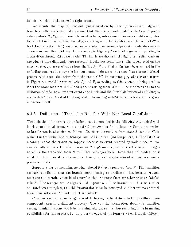
86 8. Discussion of Some Issues in the Semanticsits left branch and the other its right branch.We denote this required control synchronisation by labeling next-event edges atbranches with predicates. We assume that there is an unbounded collection of predi-cate symbols P1; P2; : : :, di�erent from all other symbols used. Given a condition symbolfor which there exist at least two MSCs starting with that symbol (e.g. the symbol C2 inboth Figures 2.6 and 8.1), we label corresponding next-event edges with predicate symbolsas we construct the unfolding. For example, in Figure 8.2 we label edges corresponding toa transition through C2 as we unfold. The labels are shown in the �gure using diamonds onthe edges (these diamonds here represent labels, not conditions). The labels used on thenext-event edges are predicates from the list P1; P2; : : : that so far have been unused in theunfolding construction, say the �rst such ones. Labels are the same if each branch of eachprocess with that label arises from the same MSC. In our example, labels P and Q usedin Figure 8.2 would be respectively P1 and P2 according to this scheme, P being used tolabel the branches from MSC2 and Q those arising from MSC3. The modi�cations to thede�nition of MSC to allow next-event edge-labels and the formal de�nition of unfolding toaccomplish this method of handling control branching in MSC speci�cations will be givenin Section 8.2.3.8.2.3 De�nition of Transition Relation With Non-Local ConditionsThe de�nition of the transition relation must be modi�ed in the following way to deal withlabeled conditional branches in a pbMFG (see Section 7.4). These predicates are neededto handle non-local choice conditions. Consider a transition from state S to state S0, inwhich the transition occurs through node u in process (ne-component) A. The intuitivemeaning is that the transition happens because an event denoted by node u occurs. Wecan formally de�ne a transition to occur through node u just in case the only out-edgesadded in the transition from S to S0 are out-edges to u. Note that ne in-edges to umust also be removed in a transition through u, and maybe also other in-edges from apredecessor of u.Suppose u has an incoming ne edge labeled P that is removed from S. The transitionthrough u indicates that the branch corresponding to predicate P has been taken, andrepresents a potentially non-local control choice. Suppose there are other ne edges labeledP in S. These edges are ne-edges to other processes. The branch on P has been takenon transition through u, and this information must be conveyed to other processes whichhave a control choice to make which includes P.Consider such an edge hx; yi labeled P, belonging to state S but in a di�erent ne-component (thus in a di�erent process). One way the information about the transitionthrough umight be conveyed is by retaining edge hx; yi in S0, but removing other branchingpossibilities for this process, i.e. all other ne edges of the form hx; �i with labels di�erent

8.2 Conditions and Non-Local Choice 87from P are removed in the transition from S to S0. This technical device retains the �nite-state character, however, it is inappropriate for the following reason. Consider the case inwhich the node u is part of a loop in the MFG. Transitions in this loop can potentially occurunboundedly often, and although this time the transition through u, and thus on predicateP, has occurred, other processes may not be on the same iteration through the loop. Inparticular the process containing x may be on some earlier iteration, on which a di�erentchoice of control branch had been made. Thus it would be inappropriate to remove thenon-P ne out-edges from x, on a transition through u as suggested above, without knowingwhich iteration each process was on. Some processes may reach a particular control branchchoice later than others, because of the asynchronous communication, thus some historyof control branch choices must be retained.Retaining the history of control branch choices necessitates the use of control historyvariables or their equivalent. History variables could be used as follows to maintain thehistory of control branch choices. A global list of control predicates is created by consec-utive choices of branching control that are made. De�ne the control vocabulary of eachprocess to be those control predicates which it uses. Associated with each process B is asublist of the global list, consisting of some tail of the global list restricted to the controlvocabulary of B, de�ned below. Call this list the B-list. The B-list is maintained in thefollowing way. As a predicate P is added to the global list, it is added to a particularB-list if and only if P is in the control vocabulary of B. When control transitions through anode u of B which involves branching control, it must transition along that ne edge whosepredicate matches that at the head of the B-list, and at the same time the head of theB-list is removed from the B-list.As we will show in more detail in Section 8.2.4 maintenance of the B-lists leads di-rectly to a non-�nite-state (in fact non-context-free) semantics. Thus such use of controlpredicates contravenes our desire to maintain a �nite-state semantics.8.2.4 Non-Local Choice May Imply Non-Finite-State ControlIf it is argued that asynchronous message-passing is non-�nite-state, the reason given isusually that message bu�ers are potentially unbounded, and that the state of the systemmust include the state of the message bu�ers. It is often granted that computation withina process may be �nite-state. However, if conditions are allowed in MFGs, then some sys-tems described by MFGs require non-�nite-state computation within individual processes.Speci�cally, either unbounded history variables are required to keep track of choices madeon conditions, or certain very simple MFGs with conditions that require non-local choice,such as those in Figure 8.1, must be regarded as ill-formed.The set of MFGs in Figure 8.1 may represent a higher-level requirement on systembehavior. A system implementing this behavior must conform to the requirement. Let us

88 8. Discussion of Some Issues in the Semanticssuppose that the implementation may perform some rudimentary amount of error recoveryon, say, temporary loss of transmission, such that the system continues to satisfy the MSCrequirement.We refer to the process whose `line' is on the left [resp. right] in Figures 8.1 and 8.2as the `left' [resp. `right'] process. Suppose we label the left branches of both processes inthe MFG in Figure 8.2 with P , to represent a choice of continuation with MSC2, and theright branches of both processes with Q to represent a continuation with MSC3. Supposenow that the system executes a trace in which the successive choices between continuationwith MSC2 and MSC3 are made as follows: 1 P choice, followed by 2 successive Q choices,then 3 successive P , then 4 successive Q, then 5 successive P , ...... The semantics ofasynchronous communication allows the the left process to fall arbitrarily behind theright process. Somehow, the history of control choices made by the right process must beknown by the left process, in order that the left process `knows' which type of messageto receive next. Suppose that the history of the last n control choices in each process isretained, in a `history variable', which we can assume is an array of length n. After atmost �k�nk = n:(n + 1)=2 branch choices, the history array contains either (a) all P 's;(b) all Q's; or (c) at most one change from P 's to Q's or vice versa. It is easy to see thereare 2:(n � 1) such possibilities for (c), which along with (a) and (b) yields 2:n possiblecon�gurations of the history variable after n:(n� 1)=2 branch choices.Suppose a recoverable fault occurs, and the system is restarted with (i) all messagebu�ers intact as when the fault occurred; (ii) all data (including history variables) intact;(iii) program counters in the same position. Suppose the fault has occurred after somewhatmore than n:(n�1)=2 branch choices. There are only 2:n possibilities for the con�gurationof the history variables in each process. Hence there are only (2:n)2 total pairs of valuesof both history variables. Suppose there are k outstanding messages. It is easy to showthat there are in�nitely many possibilities of the choice history of each process compatiblewith each given con�guration of the two history variables plus the number of outstandingmessages. However, because of the construction of the example, unless the two processesstart in corresponding places in the choice history, they will not ful�l the requirementexpressed by the MSCs in Figure 8.1.Importantly, not only the control branching history of that process but also the historyof other processes that are `further ahead', in order that the current process may makethe same control branches! To ensure that this condition is ful�lled, under even these mildrecovery conditions, either (a) the process must have an implicit means of communicatingwith the environment in order to access this history, which is held somehow by the envi-ronment in a history variable; or if not then (b) the environment must communicate thisinformation implicitly to a process as it happens, and the process must itself retain thisentire history in a variable, which must be of potentially unbounded size.These conclusions reveal highly unsatisfactory semantic situations, since they require

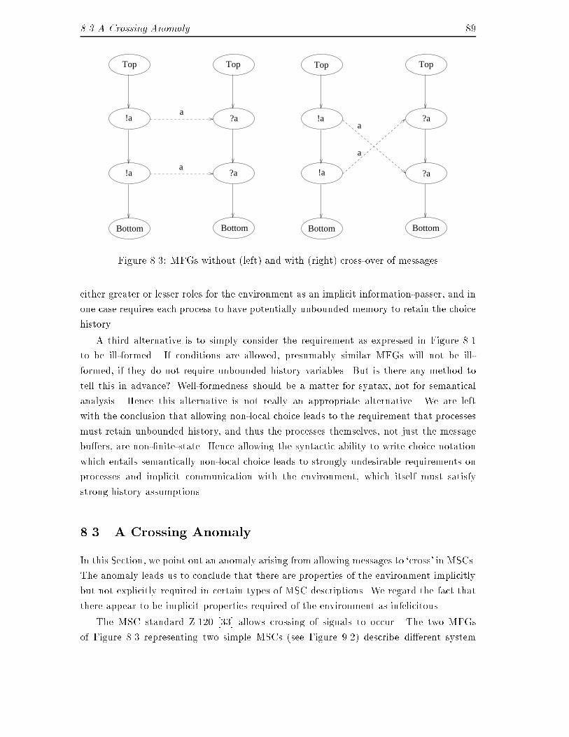
8.3 A Crossing Anomaly 89a

a

Top Top

?a!a

!a ?a

Bottom Bottom

a

Top Top

!a ?a

!a ?a

Bottom Bottom

aFigure 8.3: MFGs without (left) and with (right) cross-over of messageseither greater or lesser roles for the environment as an implicit information-passer, and inone case requires each process to have potentially unbounded memory to retain the choicehistory.A third alternative is to simply consider the requirement as expressed in Figure 8.1to be ill-formed. If conditions are allowed, presumably similar MFGs will not be ill-formed, if they do not require unbounded history variables. But is there any method totell this in advance? Well-formedness should be a matter for syntax, not for semanticalanalysis. Hence this alternative is not really an appropriate alternative. We are leftwith the conclusion that allowing non-local choice leads to the requirement that processesmust retain unbounded history, and thus the processes themselves, not just the messagebu�ers, are non-�nite-state. Hence allowing the syntactic ability to write choice notationwhich entails semantically non-local choice leads to strongly undesirable requirements onprocesses and implicit communication with the environment, which itself must satisfystrong history assumptions.8.3 A Crossing AnomalyIn this Section, we point out an anomaly arising from allowing messages to `cross' in MSCs.The anomaly leads us to conclude that there are properties of the environment implicitlybut not explicitly required in certain types of MSC descriptions. We regard the fact thatthere appear to be implicit properties required of the environment as infelicitous.The MSC standard Z.120 [33] allows crossing of signals to occur. The two MFGsof Figure 8.3 representing two simple MSCs (see Figure 9.2) describe di�erent system

90 8. Discussion of Some Issues in the Semanticsbehaviors. In both cases an identical type of signal is transmitted twice. The second casedi�ers from the �rst in that a `cross-over' of the messages is speci�ed. The observablebehavior of each individual process is identical in the two examples (one sends two `a'signals, the other receives two `a' signals), hence code implementing each process will beidentical in both examples. However, the two examples have di�erent sets of valid traces.The set of traces (interleaved observable events) of the �rst MSC is f<!a; !a; ?a; ?a >,<!a; ?a; !a; ?a >g, and that of the second is is f<!a; !a; ?a; ?a >g. A system exhibitingbehavior <!a; ?a; !a; ?a > satis�es the �rst speci�cation but not the second. However, asystem exhibiting behavior f<!a; !a; ?a; ?a >g and no other may satisfy either speci�cation.Since there is no di�erence in process code for the two examples, the di�erent tracesets must be accounted for by a di�erence in the behavior of the environment. Thus, eventhough the environment is not explicitly represented in this speci�cation, its propertiesmust be invoked implicitly. One may try to resolve this problem by representing theenvironment explicitly, as a single vertical line like a process axis, provided it engages inmessage interaction with the processes (cf. [28]). However, this is no solution. Even ifthe environment is explicitly represented as such a third axis, �rstly one can still obtainanalogous process behavior by using cross-overs, and secondly this behavior may only beobtained by using a cross-over.One criterion for a good speci�cation method (to distinguish it, say, from the averageprogramming language) is that all asserted properties be represented explicitly, includingconstraints from the environment. Our example shows that MSCs with cross-over donot pass this test. Further, even if the environment is explicit, cross-over is at best anunintuitive method of enforcing certain orderings on behavior, for which there is no otherrepresentation mechanism. Such `programming tricks' have no place in a good descriptionmethod.8.4 MSC Speci�cations can `Count' Receptions.We now show that MSCs can `count' receptions, which was pointed out in Chapter 5,where we used this ability to argue for the possibility of individuation of �nitely manymessages in an MFG, to be a feature which is a non-anomalous, expected consequence ofa semantics, even though intuitively it may appear strange.The example arises from our requirement that processes engage in �nite-state controlbehavior with regard to messages (Chapter 5). Compare MSC I, Figure 2.2, with MSCIV, Figure 2.5. Both examples express a non-terminating send of a signal of type a fromthe �rst process to the second, so at �rst glance one might imagine that they de�ne thesame set of traces. However, in MSC I, taking a ?a action removes the edge hy; zi from thestate, and thus disables a further ?a action until after a further !a action has put the edgeback in the state. Thus there may be no two consecutive receives, although there may

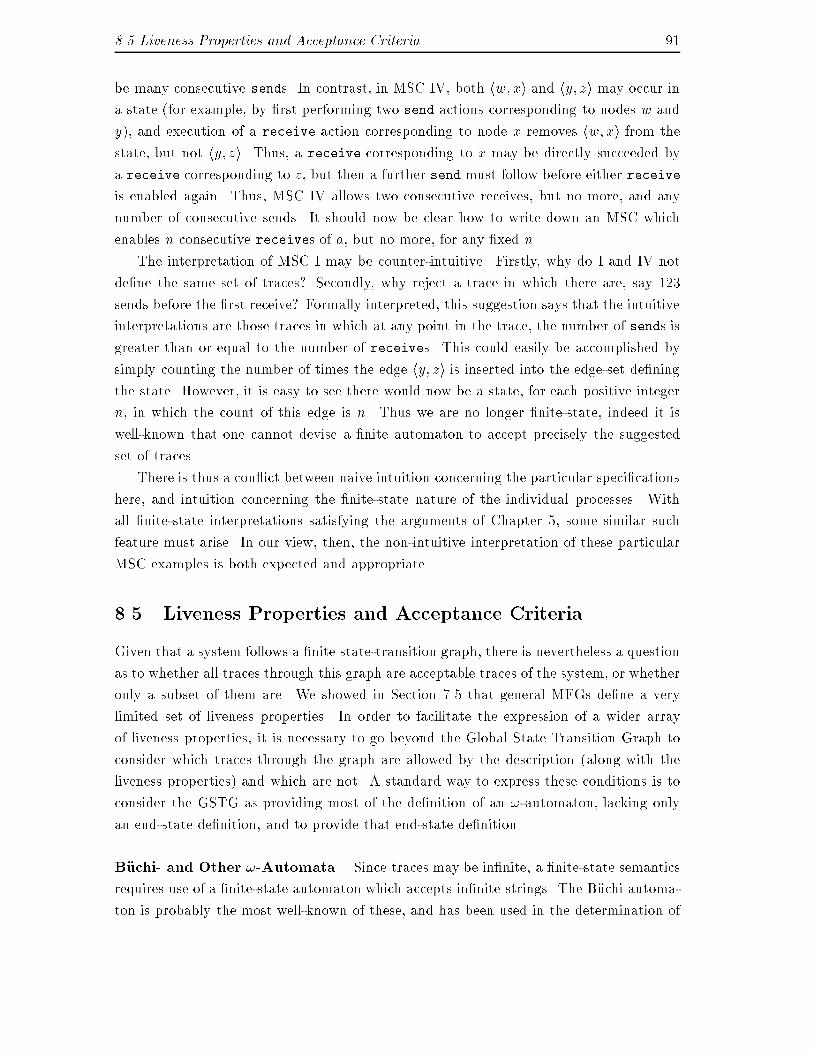
8.5 Liveness Properties and Acceptance Criteria 91be many consecutive sends. In contrast, in MSC IV, both hw; xi and hy; zi may occur ina state (for example, by �rst performing two send actions corresponding to nodes w andy), and execution of a receive action corresponding to node x removes hw; xi from thestate, but not hy; zi. Thus, a receive corresponding to x may be directly succeeded bya receive corresponding to z, but then a further send must follow before either receiveis enabled again. Thus, MSC IV allows two consecutive receives, but no more, and anynumber of consecutive sends. It should now be clear how to write down an MSC whichenables n consecutive receives of a, but no more, for any �xed n.The interpretation of MSC I may be counter-intuitive. Firstly, why do I and IV notde�ne the same set of traces? Secondly, why reject a trace in which there are, say 123sends before the �rst receive? Formally interpreted, this suggestion says that the intuitiveinterpretations are those traces in which at any point in the trace, the number of sends isgreater than or equal to the number of receives. This could easily be accomplished bysimply counting the number of times the edge hy; zi is inserted into the edge-set de�ningthe state. However, it is easy to see there would now be a state, for each positive integern, in which the count of this edge is n. Thus we are no longer �nite-state, indeed it iswell-known that one cannot devise a �nite automaton to accept precisely the suggestedset of traces.There is thus a con ict between naive intuition concerning the particular speci�cationshere, and intuition concerning the �nite-state nature of the individual processes. Withall �nite-state interpretations satisfying the arguments of Chapter 5, some similar suchfeature must arise. In our view, then, the non-intuitive interpretation of these particularMSC examples is both expected and appropriate.8.5 Liveness Properties and Acceptance CriteriaGiven that a system follows a �nite state-transition graph, there is nevertheless a questionas to whether all traces through this graph are acceptable traces of the system, or whetheronly a subset of them are. We showed in Section 7.5 that general MFGs de�ne a verylimited set of liveness properties. In order to facilitate the expression of a wider arrayof liveness properties, it is necessary to go beyond the Global State Transition Graph toconsider which traces through the graph are allowed by the description (along with theliveness properties) and which are not. A standard way to express these conditions is toconsider the GSTG as providing most of the de�nition of an !-automaton, lacking onlyan end-state de�nition, and to provide that end-state de�nition.B�uchi- and Other !-Automata. Since traces may be in�nite, a �nite-state semanticsrequires use of a �nite-state automaton which accepts in�nite strings. The B�uchi automa-ton is probably the most well-known of these, and has been used in the determination of

92 8. Discussion of Some Issues in the SemanticsT1 T2

!CR ?CR

!DR?DR!CC?CCS3S2

S1

S0

[!CR,?CR]

[!CR,?CR]

[!CR,?CR]

[!CC,?CC]

[!DR,?DR]Figure 8.4: A MFG and the corresponding GSTG whose liveness may not be speci�ed byB�uchi acceptancesafety and liveness properties of distributed systems [8], [9]. As mentioned earlier, theseautomata are similar to ordinary �nite automata, except for the acceptance condition.B�uchi automata include in their de�nition a set of states called the end-state set. A (pos-sibly in�nite) string is accepted by a B�uchi automaton just in case the automaton passesthrough an end state unboundedly often on the string (for �nite strings, the �nal statemust be an end state).Given a general MFG speci�cation, involving a family of MFGs with conditions, theGSTG is uniquely determined. From this graph, various di�erent end-state de�nitionswill de�ne various di�erent !-automata, each of which identi�es the set of system tracesspeci�ed by the MFG with the set of accepted traces of the automaton. The Global-State Transition Graph itself de�nes a B�uchi automaton, namely the one in which theend-states are the set of all states. Even though B�uchi automata de�ne a very rich classof trace-sets (in fact, they express a �11-complete set), in order to use them exibly onemust be at liberty freely to design the state set. We are constrained by having to use theglobal states de�ned in the GSTG, and we show now that the B�uchi acceptance conditiondoes not su�ce to de�ne certain natural liveness conditions, given the GSTG states andtransitions. Therefore other acceptance conditions may be preferable.B�uchi automata are su�cient to describe liveness properties of systems, provided thatthe speci�er is free to choose the states of the automaton during the course of designing anautomaton to accept precisely the desired traces. However, the global states of an MFGare speci�ed, uniquely, by the MFG. We are not free to choose an alternative state set3.If one needs to specify liveness properties of an MFG description, the de�nition of B�uchiacceptance may not su�ce. Consider the GSTG on the right hand side of in Figure 8.4,3It may be possible to devise a general transformation of a GSTG into another GSTG G0 satisfyingidentical safety properties such that a di�erent set of of liveness properties may be de�ned for G0 based onB�uchi acceptance. However, we do not know of one, or whether such a transformation might have otherdisadvantages.

8.5 Liveness Properties and Acceptance Criteria 93derived from the MFG on the left hand side in the same Figure4. It represents a systemwhich when in state S1 makes a non-deterministic choice between transiting into twostates S2 and S3, and then returns to state S1. A important liveness property may be torequire that the system performs a fair choice between the subbehaviours S2 and S3. Thisis expressed in temporal logic as (23at S2 ^ 23at S3)5. It is easy to see that there isno set of end-states under which this liveness condition is expressed by B�uchi acceptance(just look at the 15 possible non-trivial end-state sets).We conclude that the proper de�nition of liveness properties for the GSTG and there-fore for the system described by the MFGs may be accomplished better by temporal logicformulae than by B�uchi acceptance. This is because the design of the B�uchi automatonis constrained by the necessary selection of a particular transition graph, the GSTG. Itremains to be seen whether other acceptance criteria su�ce to de�ne automata suitablefor all potential liveness criteria. In the meantime, temporal logic appears to be able tode�ne the liveness criteria which users of MFGs may want. We have de�ned the preciserelationship between temporal logic assertions and MFG `executions' in Section 7.6.

4Note that the signal arrows in this MFG indicate synchronous communication, since we can make ourpoint with this GSTG, which is much simpler than that derived from the same MFG with asynchronouscommunication. This may be another indication that life with synchronous communication is easier.5As described in [113], at S2 and at S3 are state predicates asserting that the system is in state S2 orS3, respectively.

Chapter 9Semantic Features of MSCs inZ.120As mentioned before, standard MSCs are de�ned as an activity of the ITU-T standardiza-tion body, formulated in standard document Z.120. We note here some di�erences betweenan interpretation consistent with our requirements and some comments in Z.120, the cur-rent standard on MSCs. We do not regard this as a disadvantage of our semantics, butrather as a demonstration of the need for further formal analysis of the meaning of MSCs.There is no formal description of a semantics in Z.120, but some informal explanationsare given. Our comments refer to what we understand from these informal explanations1.9.1 Commentary on Z.1209.1.1 MSCs and SDLAlthough MFGs are sometimes used in their MSC form in combination with SDL [32],we consider them an independent technique. Examples of use of MFGs independently ofSDL are [140, 147, 132, 84, 137, 96, 100] (see also Chapter 3). We think it unwise torestrict ourselves to uses in the context of SDL. It is thus in exible to de�ne an MSCas representing a set of traces of an SDL-speci�cation, as in Z.120. In our semantics, anMSC de�nes a set of traces of send and receive events for the message types speci�edin the MSC de�nition. This allows MSCs to be given meaning independent of an SDLspeci�cation, while remaining consistent with an interpretation in an SDL context, andaccruing no disadvantages that we can see.1A semantics for MSCs has recently been standardised and added as Annex B to the Z.120 document.For a discussion of this semantics see Section 10.1.

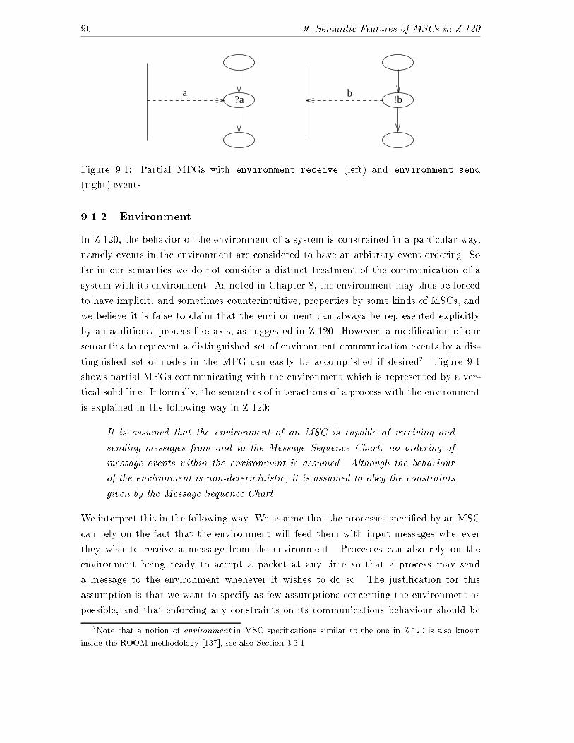
96 9. Semantic Features of MSCs in Z.120!b?a

a bFigure 9.1: Partial MFGs with environment receive (left) and environment send(right) events9.1.2 EnvironmentIn Z.120, the behavior of the environment of a system is constrained in a particular way,namely events in the environment are considered to have an arbitrary event ordering. Sofar in our semantics we do not consider a distinct treatment of the communication of asystem with its environment. As noted in Chapter 8, the environment may thus be forcedto have implicit, and sometimes counterintuitive, properties by some kinds of MSCs, andwe believe it is false to claim that the environment can always be represented explicitlyby an additional process-like axis, as suggested in Z.120. However, a modi�cation of oursemantics to represent a distinguished set of environment communication events by a dis-tinguished set of nodes in the MFG can easily be accomplished if desired2. Figure 9.1shows partial MFGs communicating with the environment which is represented by a ver-tical solid line. Informally, the semantics of interactions of a process with the environmentis explained in the following way in Z.120:It is assumed that the environment of an MSC is capable of receiving andsending messages from and to the Message Sequence Chart; no ordering ofmessage events within the environment is assumed. Although the behaviourof the environment is non-deterministic, it is assumed to obey the constraintsgiven by the Message Sequence Chart.We interpret this in the following way. We assume that the processes speci�ed by an MSCcan rely on the fact that the environment will feed them with input messages wheneverthey wish to receive a message from the environment. Processes can also rely on theenvironment being ready to accept a packet at any time so that a process may senda message to the environment whenever it wishes to do so. The justi�cation for thisassumption is that we want to specify as few assumptions concerning the environment aspossible, and that enforcing any constraints on its communications behaviour should be2Note that a notion of environment in MSC speci�cations similar to the one in Z.120 is also knowninside the ROOM methodology [137], see also Section 3.3.1.

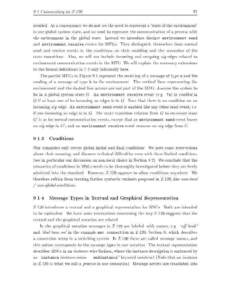
9.1 Commentary on Z.120 97avoided. As a consequence we do not see the need to represent a `state of the environment'in our global system state, and no need to represent the communication of a process withthe environment in the global state. Instead we introduce distinct environment sendand environment receive events for MFGs. They distinguish themselves from normalsend and receive events in the conditions on their enabling and the semantics of thestate transitions. Also, we will not include incoming and outgoing sig edges related toenvironment communication events in the MFG. We will explain the necessary extensionsto the formal de�nitions in 7.4 only informally here.The partial MFGs in Figure 9.1 represent the receiving of a message of type a and thesending of a message of type b to the environment. The vertical lines representing theenvironment and the dashed line arrows are not part of the MFG. Assume the system tobe in a global system state G. An environment receive event (e.g. ?a) is enabled inG if at least one of its incoming ne edges is in G. Note that there is no condition on anincoming sig edge. An environment send event is enabled like any other send event, i.e.if one incoming ne edge is in G. The state transition relation from G to successor stateG0 is as for normal communication events, except that an environment send event leavesno sig edge in G0, and an environment receive event removes no sig edge from G.9.1.3 ConditionsOur semantics only covers global initial and �nal conditions. We note some reservationsabout their meaning, and discover technical di�culties even with these limited conditions(see in particular our discussion on non-local choice in Section 8.2). We conclude that thesemantics of conditions in MSCs needs to be thoroughly investigated before they are freelyadmitted into the standard. However, Z.120 appears to allow conditions anywhere. Wetherefore refrain from treating further syntactic variants proposed in Z.120, like non-local/ non-global conditions.9.1.4 Message Types in Textual and Graphical RepresentationZ.120 introduces a textual and a graphical representation for MSCs. Both are intendedto be equivalent. We have some reservations concerning the way Z.120 suggests that thetextual and the graphical notation are related.In the graphical notation messages in Z.120 are labeled with names, e.g. `o� hook'and `dial tone on' in the example msc connection in Z.120, Section 6, which describesa connection setup in a switching system. In Z.120 these are called message names, andthis notion corresponds to the message types in our notation. The textual representationdescribes MSCs in an instance-wise fashion, where the instance description is embraced byan \instance instance-name ... endinstance" keyword construct (Note that an instancein Z.120 is what we call a process in our semantics). Message arrows are translated into

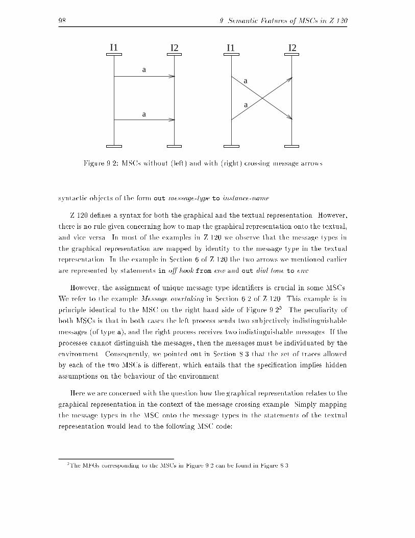
98 9. Semantic Features of MSCs in Z.120a

a

a

a

I1 I2 I1 I2

Figure 9.2: MSCs without (left) and with (right) crossing message arrowssyntactic objects of the form out message-type to instance-name.Z.120 de�nes a syntax for both the graphical and the textual representation. However,there is no rule given concerning how to map the graphical representation onto the textual,and vice versa. In most of the examples in Z.120 we observe that the message types inthe graphical representation are mapped by identity to the message type in the textualrepresentation. In the example in Section 6 of Z.120 the two arrows we mentioned earlierare represented by statements in o� hook from env and out dial tone to env.However, the assignment of unique message type identi�ers is crucial in some MSCs.We refer to the example Message overtaking in Section 6.2 of Z.120. This example is inprinciple identical to the MSC on the right hand side of Figure 9.23. The peculiarity ofboth MSCs is that in both cases the left process sends two subjectively indistinguishablemessages (of type a), and the right process receives two indistinguishable messages. If theprocesses cannot distinguish the messages, then the messages must be individuated by theenvironment. Consequently, we pointed out in Section 8.3 that the set of traces allowedby each of the two MSCs is di�erent, which entails that the speci�cation implies hiddenassumptions on the behaviour of the environment.Here we are concerned with the question how the graphical representation relates to thegraphical representation in the context of the message crossing example. Simply mappingthe message types in the MSC onto the message types in the statements of the textualrepresentation would lead to the following MSC code:3The MFGs corresponding to the MSCs in Figure 9.2 can be found in Figure 8.3.

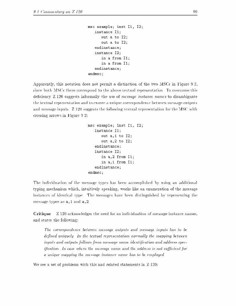
9.1 Commentary on Z.120 99msc example; inst I1, I2;instance I1;out a to I2;out a to I2;endinstance;instance I2;in a from I1;in a from I1;endinstance;endmsc;Apparently, this notation does not permit a distinction of the two MSCs in Figure 9.2,since both MSCs there correspond to the above textual representation. To overcome thisde�ciency Z.120 suggests informally the use of message instance names to disambiguatethe textual representation and to ensure a unique correspondence between message outputsand message inputs. Z.120 suggests the following textual representation for the MSC withcrossing arrows in Figure 9.2:msc example; inst I1, I2;instance I1;out a,1 to I2;out a,2 to I2;endinstance;instance I2;in a,2 from I1;in a,1 from I1;endinstance;endmsc;The individuation of the message types has been accomplished by using an additionaltyping mechanism which, intuitively speaking, works like an enumeration of the messageinstances of identical type. The messages have been distinguished by representing themessage types as a,1 and a,2.Critique. Z.120 acknowledges the need for an individuation of message instance names,and states the following:The correspondence between message outputs and message inputs has to bede�ned uniquely. In the textual representation normally the mapping betweeninputs and outputs follows from message name identi�cation and address spec-i�cation. In case where the message name and the address is not su�cient fora unique mapping the message instance name has to be employed.We see a set of problems with this and related statements in Z.120:

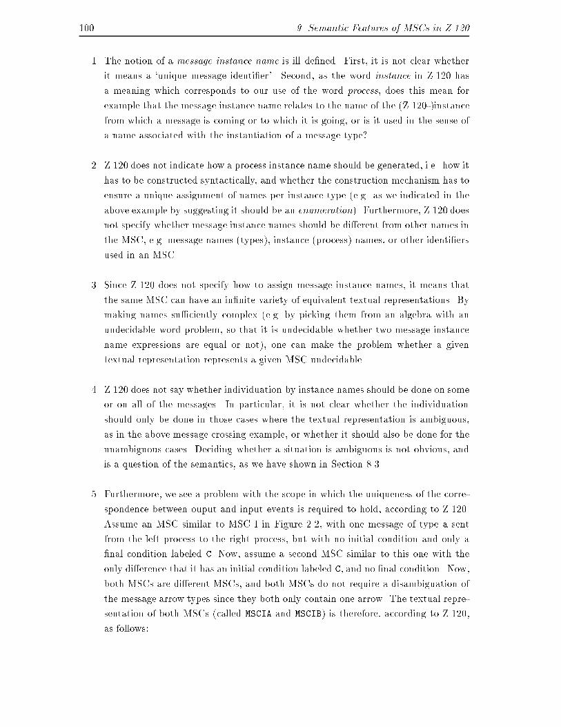
100 9. Semantic Features of MSCs in Z.1201. The notion of a message instance name is ill de�ned. First, it is not clear whetherit means a `unique message identi�er'. Second, as the word instance in Z.120 hasa meaning which corresponds to our use of the word process, does this mean forexample that the message instance name relates to the name of the (Z.120-)instancefrom which a message is coming or to which it is going, or is it used in the sense ofa name associated with the instantiation of a message type?2. Z.120 does not indicate how a process instance name should be generated, i.e. how ithas to be constructed syntactically, and whether the construction mechanism has toensure a unique assignment of names per instance type (e.g. as we indicated in theabove example by suggesting it should be an enumeration). Furthermore, Z.120 doesnot specify whether message instance names should be di�erent from other names inthe MSC, e.g. message names (types), instance (process) names, or other identi�ersused in an MSC.3. Since Z.120 does not specify how to assign message instance names, it means thatthe same MSC can have an in�nite variety of equivalent textual representations. Bymaking names su�ciently complex (e.g. by picking them from an algebra with anundecidable word problem, so that it is undecidable whether two message instancename expressions are equal or not), one can make the problem whether a giventextual representation represents a given MSC undecidable.4. Z.120 does not say whether individuation by instance names should be done on someor on all of the messages. In particular, it is not clear whether the individuationshould only be done in those cases where the textual representation is ambiguous,as in the above message crossing example, or whether it should also be done for theunambiguous cases. Deciding whether a situation is ambiguous is not obvious, andis a question of the semantics, as we have shown in Section 8.3.5. Furthermore, we see a problem with the scope in which the uniqueness of the corre-spondence between ouput and input events is required to hold, according to Z.120.Assume an MSC similar to MSC I in Figure 2.2, with one message of type a sentfrom the left process to the right process, but with no initial condition and only a�nal condition labeled C. Now, assume a second MSC similar to this one with theonly di�erence that it has an initial condition labeled C, and no �nal condition. Now,both MSCs are di�erent MSCs, and both MSCs do not require a disambiguation ofthe message arrow types since they both only contain one arrow. The textual repre-sentation of both MSCs (called MSCIA and MSCIB) is therefore, according to Z.120,as follows:

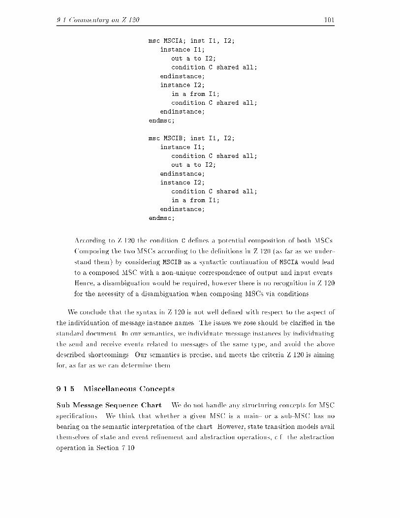
9.1 Commentary on Z.120 101msc MSCIA; inst I1, I2;instance I1;out a to I2;condition C shared all;endinstance;instance I2;in a from I1;condition C shared all;endinstance;endmsc;msc MSCIB; inst I1, I2;instance I1;condition C shared all;out a to I2;endinstance;instance I2;condition C shared all;in a from I1;endinstance;endmsc;According to Z.120 the condition C de�nes a potential composition of both MSCs.Composing the two MSCs according to the de�nitions in Z.120 (as far as we under-stand them) by considering MSCIB as a syntactic continuation of MSCIA would leadto a composed MSC with a non-unique correspondence of output and input events.Hence, a disambiguation would be required, however there is no recognition in Z.120for the necessity of a disambiguation when composing MSCs via conditions.We conclude that the syntax in Z.120 is not well de�ned with respect to the aspect ofthe individuation of message instance names. The issues we rose should be clari�ed in thestandard document. In our semantics, we individuate message instances by individuatingthe send and receive events related to messages of the same type, and avoid the abovedescribed shortcomings. Our semantics is precise, and meets the criteria Z.120 is aimingfor, as far as we can determine them.9.1.5 Miscellaneous ConceptsSub Message Sequence Chart. We do not handle any structuring concepts for MSCspeci�cations. We think that whether a given MSC is a main- or a sub-MSC has nobearing on the semantic interpretation of the chart. However, state transition models availthemselves of state and event re�nement and abstraction operations, c.f. the abstractionoperation in Section 7.10.

102 9. Semantic Features of MSCs in Z.120Abstraction. We do not consider re�nement and abstraction corresponding to the pro-cess and sub-MSC concepts of Z.120.Process model. The process model discussed employed in our semantics is static, with-out dynamic generation of processes. However, it may easily be modi�ed to include dy-namic process generation, in the following way. A create instruction to generate a processis introduced as a node in the MFG. Its meaning would be similar to the semantics of asynchronous communication. The predecessor node of a node corresponding to a createreceive event may only be a Top node. The termination of an instance, in Z.120 calledprocess stop, can be treated similarly.Coregion. Events along instance axes are totally ordered in our approach. We have noconcept comparable to the coregion of Z.120. A treatment of the coregion concept couldbe accomplished similarly to the treatment of the event ordering for the environment,allowing for an arbitrary interleaving of events in the coregion with any other event in thesystem.Timer. We do not address the timer concept in Z.120 here. However, [117] presents analgorithm for the veri�cation of real-time constraint annotated MSCs, and in Part III wewill discuss the use of real-time temporal logic for the speci�cation of real-time constraintsfor MSCs.Parameter Lists. Z.120 allows messages to be parametrized. However, there is no dataconcept in MSCs, and thus no data type mechanisms are available. We conclude thatthere can be only �nitely many di�erent parameter lists in an MSC speci�cation, and wede�ne the parameter lists to be part of the message types.Instance Names. Z.120 uses in both the graphical and the textual representation pro-cess names (there called instance names). We do not include instance names into oursemantics. However, we noted that processes form connected components of the ne re-lation in MFGs (see Section 7.2), and it is straightforward to de�ne a labeling of eachconnected component of the MFG into a name alphabet4. Figure 9.2 shows an exampleof two MSCs where the instances have been named I1 and I2, respectively.Action. Z.120 introduces so-called actions which represent non-communication events.We doubt that this is a useful concept as MSC and MFG speci�cations seem to focus onmessage exchanges between processes and abstract from internal computation. However,4C.f. the process name alphabet PT and the labeling function ptype in our semantics.

9.2 Global System States in Z.120 103actions can be interpreted similarly to the environment communication events we de�nedabove.9.2 Global System States in Z.120According to Z.120a global system state is determined by the values of the variables and the stateof execution of each process and the contents of the message queues.This seems to contradict the informal semantics de�nition given in Z.120, which containsno concept of data and thus no concept of variables. Furthermore, message queues arenot represented explicitly in MSCs, and we have presented an argument why this shouldremain so in Chapter 5 above.There is a further human-factors argument against incorporating potentially un-bounded message queues, as seemingly suggested in Z.120. Users of MSCs do not alwayswant to think of the states of queues in order to see what their MSCs de�ne. In contrastto many other speci�cation methods, the appeal of MSCs lies in their relatively simplegraphics for talking about sequences of messages. If determining the global system staterequired information about the contents of queues at any point in a trace, then `what yousee' in an MSC would not be `what you get', i.e. there would be non-explicit semanticinformation concerning the history of a computation that had to be taken into accountwhen determining the next state of the system. This contradicts the argument put forwardin Section 4.7. In our MSC semantics, we only employ features which are explicitly repre-sented in MSCs, thus we do not consider data, and we do not explicitly represent queues.We thus consider the above quoted global states argument of Z.120 to be misguided.

Chapter 10Alternative Approaches to aSemantics for MSCsThe syntax of MSCs has been standardized in Z.120. Various attempts have been madeto also standardise the semantics of MSCs, and ITU-T has recently added one of theseproposals as Annex B to the Z.120 standard document [83]. We have some reservationsconcerning this semantics, and we o�er a discussion and comparison with our work inSection 10.1. An approach towards the semantics based on Petri-Nets will be discussed inSection 10.2, and we will �nally mention some more approaches in Section 10.3.10.1 Comparison with an ITU-T Standardized SemanticsThe ITU document [83] standardizes a formal semantics for MSCs based on Process Al-gebra. A condensed version of the semantics appears in [114]. In the remainder we willrefer to the standards document as Z.120 Annex B, or simply as Annex B. The semanticsis based on an interpretation of the textual representation of MSCs as de�ned in Z.120.Annex B de�nes a notion of Basic Message Sequence Charts, identical to our sMFGs,which are then translated into expressions of a process algebra called PAMSC which isbased on ACP [16].10.1.1 Textual RepresentationMSCs are graphical objects arranged according to a graphical syntax. In our semantics weinterpret these graphical objects as mathematical objects, namely as labeled graphs calledMFGs, and we base the semantics directly on these graphs. In contrast to that AnnexB prefers not to interpret the graphical notation directly, but instead to use the textualrepresentation according to Z.120 as the starting point for the semantic interpretation. Wenoted in Chapter 9.1 problems with the relation of graphical to textual representation in

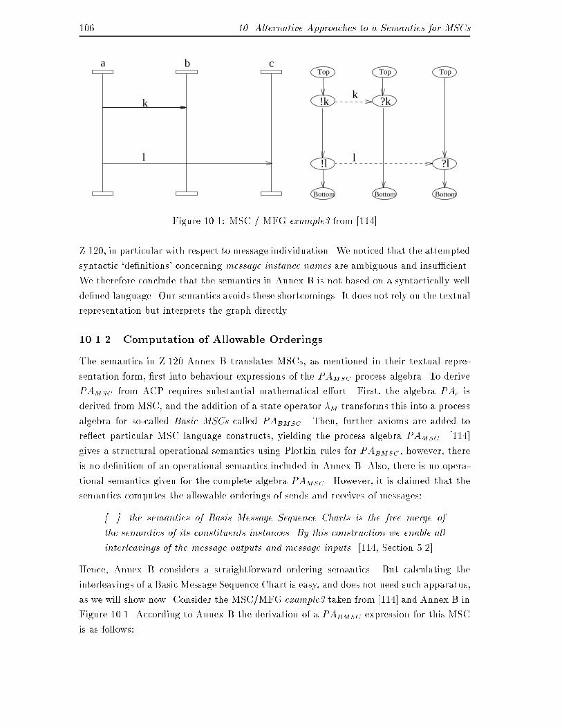
106 10. Alternative Approaches to a Semantics for MSCsBottom Bottom Bottom

l

k

TopTopTopa b c

!k ?kk

l!l ?lFigure 10.1: MSC / MFG example3 from [114]Z.120, in particular with respect to message individuation. We noticed that the attemptedsyntactic `de�nitions' concerning message instance names are ambiguous and insu�cient.We therefore conclude that the semantics in Annex B is not based on a syntactically wellde�ned language. Our semantics avoids these shortcomings. It does not rely on the textualrepresentation but interprets the graph directly.10.1.2 Computation of Allowable OrderingsThe semantics in Z.120 Annex B translates MSCs, as mentioned in their textual repre-sentation form, �rst into behaviour expressions of the PAMSC process algebra. To derivePAMSC from ACP requires substantial mathematical e�ort. First, the algebra PA� isderived from MSC, and the addition of a state operator �M transforms this into a processalgebra for so-called Basic MSCs called PABMSC . Then, further axioms are added tore ect particular MSC language constructs, yielding the process algebra PAMSC . [114]gives a structural operational semantics using Plotkin rules for PABMSC , however, thereis no de�nition of an operational semantics included in Annex B. Also, there is no opera-tional semantics given for the complete algebra PAMSC . However, it is claimed that thesemantics computes the allowable orderings of sends and receives of messages:[...] the semantics of Basis Message Sequence Charts is the free merge ofthe semantics of its constituents instances. By this construction we enable allinterleavings of the message outputs and message inputs. [114, Section 5.2]Hence, Annex B considers a straightforward ordering semantics. But calculating theinterleavings of a Basic Message Sequence Chart is easy, and does not need such apparatus,as we will show now. Consider the MSC/MFG example3 taken from [114] and Annex B inFigure 10.1. According to Annex B the derivation of a PABMSC expression for this MSCis as follows:

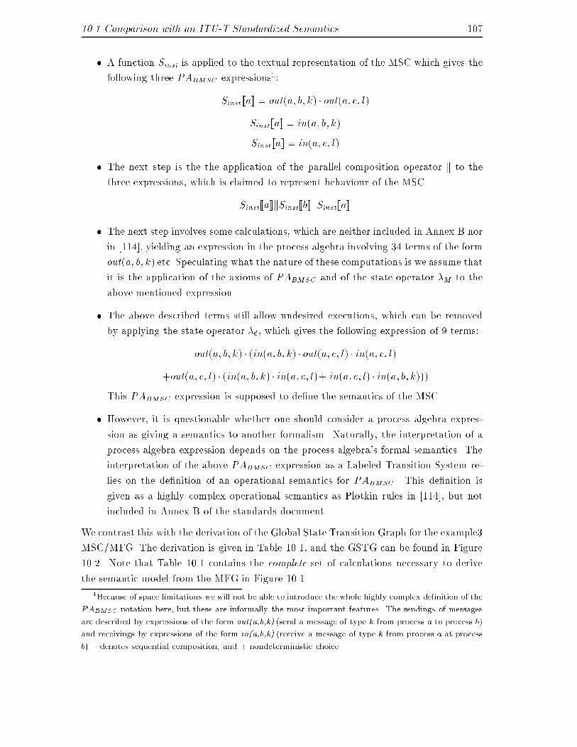
10.1 Comparison with an ITU-T Standardized Semantics 107� A function Sinst is applied to the textual representation of the MSC which gives thefollowing three PABMSC expressions1:Sinst[[a]] = out(a; b; k) � out(a; c; l)Sinst[[a]] = in(a; b; k)Sinst[[a]] = in(a; c; l)� The next step is the the application of the parallel composition operator k to thethree expressions, which is claimed to represent behaviour of the MSC.Sinst[[a]]kSinst[[b]]kSinst[[a]]� The next step involves some calculations, which are neither included in Annex B norin [114], yielding an expression in the process algebra involving 34 terms of the formout(a; b; k) etc. Speculating what the nature of these computations is we assume thatit is the application of the axioms of PABMSC and of the state operator �M to theabove mentioned expression.� The above described terms still allow undesired executions, which can be removedby applying the state operator �;, which gives the following expression of 9 terms:out(a; b; k) � (in(a; b; k) � out(a; c; l) � in(a; c; l)+out(a; c; l) � (in(a; b; k) � in(a; c; l)+ in(a; c; l) � in(a; b; k)))This PABMSC expression is supposed to de�ne the semantics of the MSC.� However, it is questionable whether one should consider a process algebra expres-sion as giving a semantics to another formalism. Naturally, the interpretation of aprocess algebra expression depends on the process algebra's formal semantics. Theinterpretation of the above PABMSC expression as a Labeled Transition System re-lies on the de�nition of an operational semantics for PABMSC . This de�nition isgiven as a highly complex operational semantics as Plotkin rules in [114], but notincluded in Annex B of the standards document.We contrast this with the derivation of the Global State Transition Graph for the example3MSC/MFG. The derivation is given in Table 10.1, and the GSTG can be found in Figure10.2. Note that Table 10.1 contains the complete set of calculations necessary to derivethe semantic model from the MFG in Figure 10.1.1Because of space limitations we will not be able to introduce the whole highly complex de�nition of thePABMSC notation here, but these are informally the most important features. The sendings of messagesare described by expressions of the form out(a,b,k) (send a message of type k from process a to process b)and receivings by expressions of the form in(a,b,k) (receive a message of type k from process a at processb). � denotes sequential composition, and + nondeterministic choice.

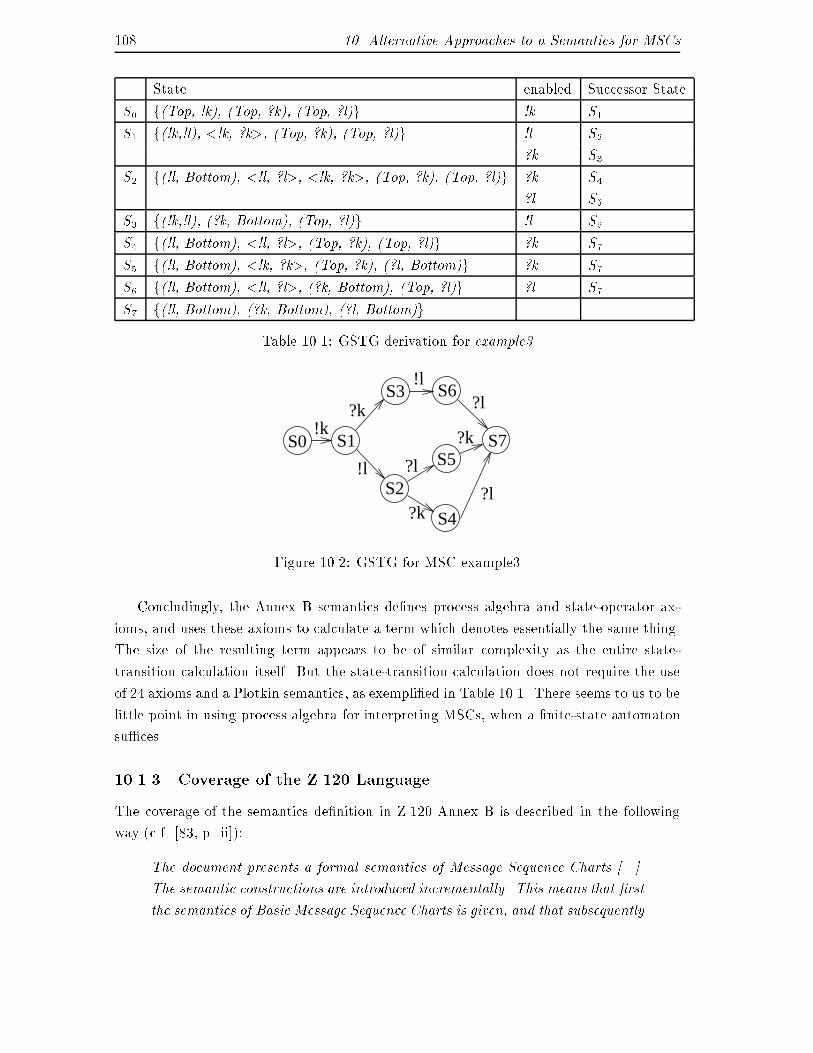
108 10. Alternative Approaches to a Semantics for MSCsState enabled Successor StateS0 f(Top, !k), (Top, ?k), (Top, ?l)g !k S1S1 f(!k,!l), <!k, ?k>, (Top, ?k), (Top, ?l)g !l S2?k S3S2 f(!l, Bottom), <!l, ?l>, <!k, ?k>, (Top, ?k), (Top, ?l)g ?k S4?l S5S3 f(!k,!l), (?k, Bottom), (Top, ?l)g !l S6S4 f(!l, Bottom), <!l, ?l>, (Top, ?k), (Top, ?l)g ?k S7S5 f(!l, Bottom), <!k, ?k>, (Top, ?k), (?l, Bottom)g ?k S7S6 f(!l, Bottom), <!l, ?l>, (?k, Bottom), (Top, ?l)g ?l S7S7 f(!l, Bottom), (?k, Bottom), (?l, Bottom)gTable 10.1: GSTG derivation for example3S0 S1

S3

S2

S5

S4

!k?k

!l ?l

!l?l

?k

?l

S6

S7

?kFigure 10.2: GSTG for MSC example3Concludingly, the Annex B semantics de�nes process algebra and state-operator ax-ioms, and uses these axioms to calculate a term which denotes essentially the same thing.The size of the resulting term appears to be of similar complexity as the entire state-transition calculation itself. But the state-transition calculation does not require the useof 24 axioms and a Plotkin semantics, as exempli�ed in Table 10.1. There seems to us to belittle point in using process algebra for interpreting MSCs, when a �nite-state automatonsu�ces.10.1.3 Coverage of the Z.120 LanguageThe coverage of the semantics de�nition in Z.120 Annex B is described in the followingway (c.f. [83, p. ii]):The document presents a formal semantics of Message Sequence Charts [...].The semantic constructions are introduced incrementally. This means that �rstthe semantics of Basic Message Sequence Charts is given, and that subsequently

10.1 Comparison with an ITU-T Standardized Semantics 109additional features are added until the complete language is covered.In other words, Annex B claims to give a semantics de�nition of the complete MSC lan-guage as de�ned in Z.120. We show that this is false. As we noted earlier, the MSCstandard includes conditions, which are to be used to `join' MSCs, in such a way thatdi�erent MSCs may describe consecutive parts of the same system execution. Basic MSCsdo not include conditions. However, as indicated above Annex B pursues an incrementalextension of the semantics, and in Section B.4.8 a treatment of conditions is consequentlydescribed. The function mapping MSC textual language constructs onto PAMSC expres-sions maps a condition symbol to the empty process �. Consequently, the explanatorytext reads:Note that the semantics of a chart containing conditions is simply the semanticsof the chart with the conditions deleted from it. [83, p. 27]This can clearly not be considered a treatment of the condition construct, and we concludethat the claim to cover \the complete language" is false. This has various implications,namely that the class of MSCs described by the resulting process algebra expression hasa trivial semantics, and that it only describes �nite, non-iterating and non-branching be-haviour. We have in our work addressed the semantics of conditions by de�ning a compo-sition operation and by interpreting the branching and iterating MFGs which potentiallyresult from the use of conditions.10.1.4 Finite-StatenessWe have argued at length in Chapter 5 that MSCs are inherently �nite-state systems.The semantics in Annex B is �nite-state, for a trivial reason: as we argued above, itonly describes �nite behaviours. However, extending the semantics in Annex B to in�nitebehaviours, e.g. by giving a meaning to iterating MSC speci�cations due to the use of con-ditions, would require means of expressiveness for in�nite behaviours. In process algebrasthis is usually accomplished by the use of recursion, and it is mathematically a non-trivialtask to restrict recursive process de�nitions to only express �nite-state equivalent systems.It is equally di�cult to show that a recursive process de�nition corresponds to a �nite-state system. Furthermore, there is evidence that the semantics as described in Annex Bis inherently non-�nite state, when extended to cover in�nite behaviours. According to[114, Section 4.2]this operator [the state operator �M , see above] remembers all message outputsthat have been executed in a set M and only allows a message input if itscorresponding message output is in that set.We see a few problems in this de�nition.

110 10. Alternative Approaches to a Semantics for MSCs� First, we doubt that this operator can allow the retention of complete executionhistories even for �nite MSCs. The de�nition of the operator as given in Table 4of [114] speci�es that when applying it to an out(a,b,l) expression, then the stringrepresenting this expression will be added to the set M of sent but not yet receivedmessages. In analogy to that the application to an in(a,b,l) expression will removethe out(a,b,l) expression from M . Now, let's look at the left MSC in Figure 9.2.Applying the de�nition of �M to this example would mean that there is an allowableexecution in which two times out(a,b,l) will be added to M , followed by just oneremoval of out(a,b,l), which means that two message sendings will be followed byone reception. It is obvious that this is not the intended semantics of the MSC inFigure 9.2. Although the functioning of the �M operator is similar to the addingof a sig edge to the current global system state in our semantics the distinctionbetween communication events and signal types in our semantics avoids the describedproblem2.� Second, if the semantics in Annex B was extended to capture in�nite executionslike our semantics, and the �M operator was actually de�ned in such a way thatit could remember a potentially unbounded number of sends of messages, then thiswould lead to a non-�nite state system3. Furthermore, as we point out in Chapter5 and Section 8.2, there is nothing in the state of any telecommunications systemimplementing a given MSC corresponding to keeping track of the system's completeexecution history.We conclude that the semantics in Annex B does not extend nicely to in�nite systems.10.1.5 PragmaticsWhen discussing the application of formalisations of MSCs the Z.120 Annex B documentstates:Tool builders can use the semantics for derivation of prototypes directly fromthe de�nitions provided or they can base their computer applications on thesede�nitions. [83, p. ii]Exactly how tool builders are supposed to derive prototypes from MSCs is not speci�ed.For example, BMSCs include no branching behavior, and we've noted that the branchingbehavior of general MSCs is incompletely and confusedly speci�ed by Z.120. However,2In our interpretation we would map the the signals in Figure 9.2 to two pairs of communication events(sig edges), say < u; v > and < x;y > where the signal type of both edges is a. We can thus add twodistinct sig edges to the current system state, < u; v > for the �rst message a, and < x;y > for the second.3For a similar argument see our discussion of non-local choice and the resulting need for potentiallyunbounded history variables in Section 8.2.

10.1 Comparison with an ITU-T Standardized Semantics 111most software includes at least one branch, with usually a clear meaning. Z.120 givesno clue how to specify such a branch. We conclude that the statement that softwaredevelopers may derive prototypes from ... is gratuitous.More particularly, we doubt that it will be possible to derive system prototypes fromMSC speci�cations because their behaviour will be of a much higher degree of complexitythan any behaviour which could be expressed by an MSC. However, we note that MSCsmay be useful for simulations of the message passing of a system, or for deriving objectcontrol state machines as in some object-oriented design methodologies (c.f. [132]). Wefeel that the models for MSC speci�cations resulting from our semantics (the Global StateTransition Graph) is much closer to any use in a software tool than those resulting fromthe semantics in Annex B, and therefore more practical. This for two reasons:� The main application of a formal semantics lies in the use of the generated semanticmodel for veri�cation purposes. Nowadays, most of the practical veri�cation is doneby so-called model-checking which entails traversals of the state graphs of systems(see for example in [74]).� As an important by-product software engineering tools may use a formalization toexecute a speci�cation by traversing the state transition graph. This may be helpfulwhen wanting to debug a speci�cation, or when animating the system's behaviour.We conclude that the ability to traverse a state transition graph is an importantrequirement for a semantics to be practical. It has been argued that a process algebramodel can be translated into a state-transition model. However, this is a non-trivialoperation4, and we do not see a point in doing so when a direct translation into a state-transition model can easily be done, as we have demonstrated by our approach. This meansthat the semantics in Annex B is much less practical than our approach, and thereforemuch less helpful in serving as a basis for computer applications, as required in Annex B.10.1.6 Communication MechanismThe Semantics in Annex B describes only asynchronous communication, which is the onlycommunication mechanism known to Z.120. However, we believe that our semantics, whichcovers both synchronous and asynchronous communication, is more exible and thereforehas a broader scope of applications, as for example in object-oriented methodologies (seeSection 3.3) which make use of both mechanisms.4C.f. the work on translating LOTOS speci�cations into state-machines described in [86].

112 10. Alternative Approaches to a Semantics for MSCs10.2 A Petri-Net based ApproachAn approach to MSC semantics based on Petri Net interpretations was suggested in [64].The example given there yields an interpretation which is easily and intuitively translatedinto a �nite-state automaton. The authors do not address many of the questions thatconcern us in our approach to a semantics, such as varying interpretations due to di�er-ent liveness properties, problems of synchronising non-determinism under composition byconditions, and assessing the expressive strength of MSC speci�cations, and they do notaddress the question of how to handle composition under conditions, as shown in Section7.2.3. One of the authors has suggested that a Petri Net-based semantics will not ingeneral be �nite-state [131]. We see this as a problem, since we argue in Chapter 4 thatMSCs are inherently �nite-state. Furthermore, using a semantics not based on �nite-statemethods may cause di�culty with proper use of MSCs inside some tools which, like theGEODE tool, assume MSCs to be �nite-state.10.3 Miscellaneous ApproachesSome further approaches to a semantics for MSCs focus on formalisations, data structures,and operations on MSCs [39] [40] [144]. However, they do not provide an operationalsemantics for MSCs in the way we do in our work. A formal interpretation of SDLappears in [28], where MSCs are introduced as ways of specifying `traces' with which agiven SDL speci�cation may be compared. MSCs in [28] seem to be regarded as more ofa test-derivation language, and are not themselves given a formal semantics therein.[48] describes a di�erent process-algebra based approach to the semantics of MSCs.It also considers only condition-free MSCs, and therefore only simple �nite behaviors. Amessage corresponds to two separate send and receive events. This is a simple translationof a �nite MSC into a �nite collection of partially ordered events.

Part IIIQuality of Service Speci�cation

Chapter 11IntroductionMany telecommunications systems engineers �nd it convenient to specify functional prop-erties of their systems using state-transition based formal description techniques like SDLor Message Sequence Charts (MSCs). However, the expressiveness of these techniques doesnot capture Quality of Service (QoS) requirements because many of these rely on real-timeconstraints which SDL and MSC speci�cation do not allow to express. However, suitablyextended temporal logics allow for a description of these requirements. We introduce amethod for the integration of functional system speci�cations given in SDL or MSC withtemporal logic based speci�cations of QoS requirements, and we call the resulting speci�ca-tions complementary speci�cations. We show how SDL and MSC speci�cations �t togetherwith temporal logic and real-time extended temporal logic speci�cations. Then we giveexamples of real-time related delay bound, delay jitter, and isochronicity constraint QoSspeci�cations. We discuss how our method helps in the speci�cation of: system perfor-mance to QoS mapping problems, of QoS negotiation mechanisms, and of QoS monitoring.Finally we hint at methods for the formal veri�cation of QoS speci�cations.Properties of Telecommunications SystemsIn telecommunications systems design, a lot of work has been devoted to using formaldescriptions for the speci�cation of functional properties of the designed systems. SDL[32] and Message Sequence Charts (MSCs) [33] are frequently used for this purpose, andthey will therefore play a central role here1.Properties are sets of observable sequences of events in a system. Many authors haveintroduced notions of safety and liveness properties, see for example [7, 8]. Safety prop-erties ensure that nothing bad happens, whereas liveness properties ensure that eventuallysomething good will happen. Informally, the requirement that a connection has to be1For an overview of the use of formal description techniques in telecommunications systems engineeringsee for example [108, 19, 145].

116 11. Introductionestablished before the data exchange may begin is describing such a functional property,according to the classi�cation in [7, 8] a safety property. Another property can be de-scribed by the requirement that whenever a message has been sent, then it will eventuallybe received which is according to [7, 8] classi�ed as a liveness property. We consider safetyand liveness properties as well as all combinations of these to be functional properties ofa system2.In addition to the functional aspects real-time mechanisms have been used in the designof protocols in order to ensure progress of the system, and also in order to detect errorslike message losses or unavailability of resources. For the use of the SDL timer mechanismin order to achieve the second goal see for example [19]. However, as we will show laterthe asynchronous SDL timer mechanism is unsuited to ensure progress of a system. Thishas also bearing on QoS aspects as far as they are related to hard real-time bounds [55],e.g. delay and delay jitter bounds for multimedia services.OverviewIn Chapter 12 we investigate the SDL timer mechanism and we observe limitations inits expressiveness; in particular with regard to the speci�cation of real-time boundedresponse properties. We recommend the use of complementary real-time temporal logicspeci�cations to remedy this pitfall. This requires providing a model for SDL speci�cationsbased on which temporal logic formulas can also be interpreted.In Chapter 13 we introduce a state transition model and show how SDL speci�cationscan be interpreted based on this model. This interpretation is similar to the interpretationof SDL speci�cations as communicating extended �nite state machines, for which somesuggestions exist in the literature (see Chapter 13). However, the existing proposals areeither informal, incomplete, or they do not adequately capture the SDL semantics, inparticular as far as the potentially iterative structure of SDL process transitions and theparticular semantics of the SDL INPUT statement are concerned.In Chapter 14 we show how temporal logics can be used in combination with SDLspeci�cations when these are interpreted based on the state transition model as de�ned inChapter 13. The underlying idea is that both the SDL speci�cation as well as the temporallogic speci�cation constrain the allowable behaviour of the system, and we require bothspeci�cations to be satis�ed by a system. We say that the temporal logic speci�cation isa complementary speci�cation of the basic SDL speci�cation. Temporal logic, however,allows for the speci�cation of state-based properties whereas we are often interested inspecifying properties of sequences of events, such as INPUT and OUTPUT events. We showin Chapter 14 how these events can be de�ned in terms of state predicates.2However, we should note that like MFG and MSC speci�cations SDL speci�cations do not expressliveness properties.

11. Introduction 117In Chapter 15 we specify a range of di�erent real-time constraint based QoS require-ments complementing SDL and MSC speci�cation examples. These include service re-sponse and message transmission delay bounds, delay jitter bounds, isochronicity relatedrequirements, and requirements on transmission rates.In Chapter 16 we exemplify how some QoS related mechanisms can be speci�ed usingour approach, like QoS negotiation and reaction to QoS guarantee violation.We conclude with a discussion in Chapter 17. Section 17.1 exempli�es the use of ourspeci�cation method in the context of system performance to QoS mapping problems. InSection 17.2 we discuss some issues concerning the formal veri�cation of QoS requirements.Related work. A wide range of literature is available on many of the topics discussedin this part of the thesis. We will mention the appropriate references in places where theyare relevant. However, some general literature on QoS should be mentioned here. Theproposed standardisation of QoS concepts in the ISO/OSI and ODP context is documentedin [82]. [90] gives a complementary overview over QoS topics.

Chapter 12A Critique of the SDL Real-TimeMechanismSDL has a built-in real-time mechanism, relying on an asynchronous timer mechanism.We will argue here that this mechanism is inexpressive with respect to the most importantclass of real-time requirements, namely hard real-time or bounded response constraints (seefor example [55] [14]). We will brie y explain why this sort of constraints is an importantrequirement for real-time systems, and we will then address the unsuitability of the SDLmechanism.12.1 Real-Time RequirementsWe introduced liveness properties as properties of a system which state that \somethinggood will eventually happen". This class of theoretically interesting properties has provedto be of limited practical use. By asserting that one can rely on the fact that when onehas requested a service, the request is eventually going to be served does not exclude thepossibility that one may need to wait a �nite but apparently limitless period of time forthe servicing of the request1. It is theoretically possible to specify situations which areperfectly \legal" from a liveness point of view but which could result in the user havingto wait for an impractically long period of time before the servicing of his request (e.g.exceeding human life expectancy !). Using liveness assertions in such an empirical mannerare clearly of little value and alternative approaches have to be considered if appositeuse is to be made of their bene�ts. It should also be pointed out that a closely relatedproblem associated with pure liveness requirements is the fact that liveness properties arenot testable [92], and which provides still further proof of the limited practical use of thisclass of properties.1For a similar argument in the context of a lift system speci�cation see [116].

120 12. A Critique of the SDL Real-Time MechanismTo overcome this problem, real-time models enforcing progress have been introduced.These models introduce the idea of the urgence of events which means that events arerequired to happen after a speci�ed period of time. This implies that we need to introducea notion of time into the so far purely untimed state and event sequence model. A suitabletimed execution model for our purposes is the model of timed traces [14], where steps insystem traces are labeled with monotonically increasing timestamps. The requirementthat a service request be serviced within t time units of the current moment in time isexpressed in the timed trace execution model as:the request will be serviced in a state Si, i � j, so that the timestamp ts(Si)di�ers from the current time stamp ts(Sj) by not more than t time units.We call such a requirement a bounded response requirement [67]. Bounded response re-quirements are crucial in many control system speci�cations, e.g. in communication pro-tocols and safety-critical systems [55]2.12.2 The SDL Real-Time MechanismReal-time is introduced into SDL by an asynchronous timer mechanism3. An SDL spec-i�cation can access the value of a global clock by reference to a variable called NOW. Thisvariable always refers to the current moment in time.Timers are similar to variables: they can be set, reset, and they can expire. A timercan be \set" in the course of a state transition by the SDL command set, usually beingset to a value greater than the current value of the system clock. For example, the SDLcommand set(now+t, T) would be used to set the value of a timer called T to a point oftime t time units greater than the current moment of time. This command is implementedby synchronously reading the global time value in variable NOW and adding the time distancevalue t, which yields the value to which the timer is set. We call a process which sets atimer the timed process.The set timer is administered by a timer process. Each time a timed process sets a timeran instance of the timer process will be generated. The timer process runs independentlyand asynchronously from the timed process. The timer process continuously compares thevalue to which the timer is set with the current global time value. When the value to whichthe timer is set is reached or exceeded, the timer process communicates the expiry to the2It is interesting to note that from a theoretical point of view the liveness property that the eventwill eventually be serviced becomes a safety property when it is transformed in such a bounded responserequirement [67]. This is due to the fact that in every state of the system it is possible to evaluate whetherthe requirement is satis�ed by the system execution up to the current state, or not. This is not possiblefor liveness properties.3For an instructive explanation of the SDL timer mechanism on which we base our discussion here see[19].

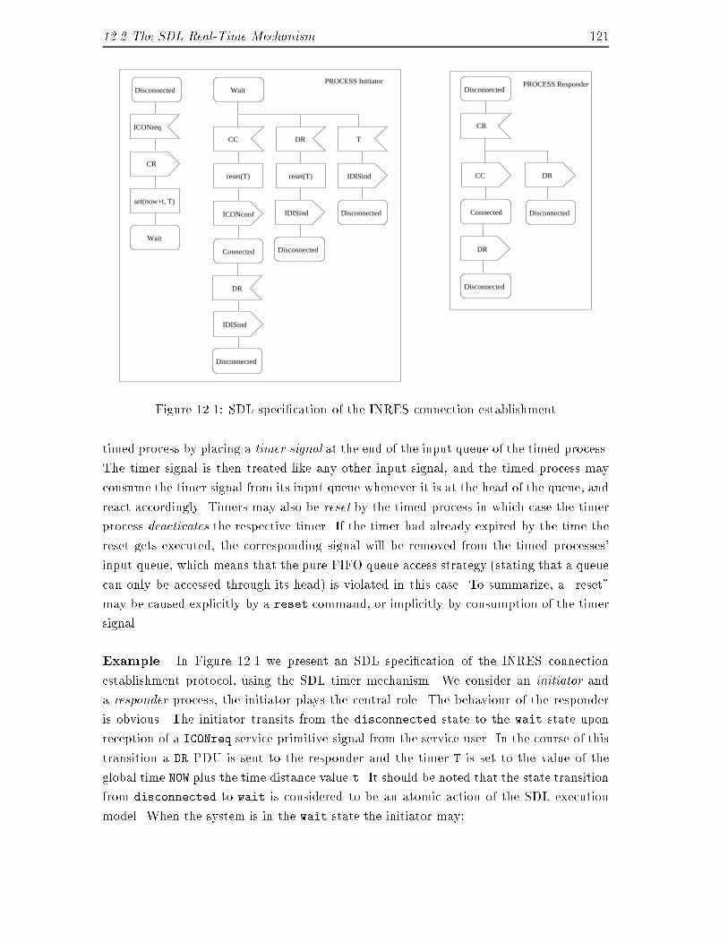
12.2 The SDL Real-Time Mechanism 121Disconnected

ICONreq

set(now+t, T)

Disconnected

Wait

Connected

CR

DR

Connected

reset(T) reset(T)

Disconnected

Disconnected

IDISind

DR

Disconnected

T

IDISind

ICONconf

DR

CC DR

Disconnected

IDISind

WaitPROCESS Initiator

Disconnected

CR

CC

PROCESS Responder

Figure 12.1: SDL speci�cation of the INRES connection establishmenttimed process by placing a timer signal at the end of the input queue of the timed process.The timer signal is then treated like any other input signal, and the timed process mayconsume the timer signal from its input queue whenever it is at the head of the queue, andreact accordingly. Timers may also be reset by the timed process in which case the timerprocess deactivates the respective timer. If the timer had already expired by the time thereset gets executed, the corresponding signal will be removed from the timed processes'input queue, which means that the pure FIFO queue access strategy (stating that a queuecan only be accessed through its head) is violated in this case. To summarize, a \reset"may be caused explicitly by a reset command, or implicitly by consumption of the timersignal.Example. In Figure 12.1 we present an SDL speci�cation of the INRES connectionestablishment protocol, using the SDL timer mechanism. We consider an initiator anda responder process, the initiator plays the central role. The behaviour of the responderis obvious. The initiator transits from the disconnected state to the wait state uponreception of a ICONreq service primitive signal from the service user. In the course of thistransition a DR PDU is sent to the responder and the timer T is set to the value of theglobal time NOW plus the time distance value t. It should be noted that the state transitionfrom disconnected to wait is considered to be an atomic action of the SDL executionmodel. When the system is in the wait state the initiator may:

122 12. A Critique of the SDL Real-Time Mechanism� receive a CC PDU from the responder, which indicates that the responder acceptsthe connection establishment, and it may then transit to state connected,� or it may receive a DR PDU which indicates a rejection of the connection request bythe responder,� or it may receive a timer signal T.After the reception of DR or T signals the initiator indicates closing of the connection orunsuccessful connection establishment respectively by issuing a IDISind service primitiveto the Initiator-user.This speci�cation example represents a very common usage of the SDL timer mech-anism in protocol speci�cations. It is generally assumed that the above use of the SDLtimer ensures progress of the system, and thereby ensures its liveness. The underlyingassumption is that the expiry of the timer forces the timed process Initiator to react,within a bounded time frame. We will now show that this assumption is false.12.3 CritiqueWe claim that the above described timer mechanism is unable to express real-time prop-erties relying on the urgence of events, as seen, for example in the bounded responserequirement introduced in Section 12.1. We consider and comment upon the followingaspects concerning the timer mechanism in SDL.� Processes receive the timer signals through their input queue. This implies that thereaction on the expiry of the timer is decoupled from the expiry itself. We maytherefore only infer that the system reacts some time after the timer expires.� Furthermore, no estimation can be made for the time it takes to consume all eventsin the queue which may (potentially) have arrived earlier than the timer signal. Thismeans that the time span between adding the timer signal to the input queue andwhen it is at the head of the queue is �nite but unbounded.� The interaction between the input queue and the process is asynchronous. Even ifa timer signal has arrived when the input queue of the timed process was emptyit cannot be guaranteed how long it will take for the timed process to actuallyconsume the timer signal and react accordingly. However, if one assumes a basictrivial liveness assumption (namely that every enabled transition will eventually betaken) then it is at least guaranteed that the reaction will eventually happen.More formally, the argument is stated as follows. Assume that at time Tnow a processsets a timer � to a time value Tnow+Tv. When the timer process expires (the system clock

12.4 Remedies 123reaches the value Tnow + Tv), then a timer expiry signal (hereafter called a timer signal)is generated. The timer signal is placed in the timed processes' input queue some T1 � 0time units later. It will be consumed (i.e. removed from the head of the receiving process'input queue) some T2 � 0 time units later by the timed process. Note that a �nite butunbounded number of messages can be in the input queue of the timed processes ahead ofthe timer signal. Note also, that depending on the structure of the speci�cation, the timedprocess may run into some state from which it will never neither reach a reset instructionnor a timer signal input statement. This will imply that at some point the timer signalwill reach the head of the timed processes' input queue, but it will be discarded and thesystem will then not react on the timer expiry at all. Finally, the earliest reaction tothe timer expiry will happen T3 � 0 time units after the consumption of the time expirysignal. This means that the delay � between the point of time when the timer expires,and the moment at which the SDL speci�cation reacts to the expiry, can be estimated as0 � � � T1 + T2 + T3, and there is no upper bound for the value of T1 + T2 + T3. Thisleads to the following points of criticism:� As there is no upper bound for the value of T1+T2+T3, it is not possible to specifya bounded response requirement using the timer mechanism.� The only property, however, which can be expressed is that before the global timehas reached the value Tnow+� the timer signal T will not be consumed. In the Inresexample this means that when the system remains in state wait, before the timeTnow + � has been reached a IDISind signal will not be issued, unless the systemhas received a CC or DR signal. It is questionable, however, whether this is a usefulproperty.We conclude that it is not possible to enforce system progress or liveness by usingthe SDL timer mechanism, and therefore that SDL does not provide an expressiveness forspecifying time-critical systems. This implies that SDL is not capable of specifying manyimportant real-time QoS requirements which rely on real-time bounds.12.4 RemediesA large number of proposals for real-time formalisms and semantics has been made inthe literature, and space limitations do not allow for a complete overview here. SDL is aspeci�cation language based on a state transition model, and the transitions are describedusing a programming language-like formalism. It therefore seems obvious here to discussapproaches to providing SDL with real-time expressiveness based on automata models andtemporal logics. We see in particular the following possibilities for a remedy of the abovedescribed shortcoming of the SDL real-time mechanism.

124 12. A Critique of the SDL Real-Time Mechanism� It has been suggested that to describe real-time constraints on state transition basedsystems may be achieved by so-called timed automata [118] [146, 111] [12, 13]. A com-mon feature of these approaches is that transitions of automata are being attributedby time constraints. Time is introduced into these systems by clock variables, andtransitions may only be taken if associated constraints on the clock values are sat-is�ed. We do not directly pursue this approach because it requires the translationof an SDL speci�cation into a state-transition system, and then to de�ne the clockvalues and constraints on them based on the state-transition model.� [18] suggest labeling SDL transitions by transition time and transition rate parame-ters. These parameters refer to time constraints on repeated executions of a transi-tion. We need a much more exible mechanism here, allowing us to specify timingconstraints referring to di�erent transitions (c.f. the discussion of the INRES exam-ple in Section 12.3), or even to events or transitions in di�erent processes. A furtherde�cit of the approach described in [18] is that no formal semantics is introduced forthe suggested constructs.� [15] suggests a method to `take a programming language o� the shelf and upgradeit into a real-time programming language'. This upgrade is accomplished by theintroduction of clock variables and a so-called guarded wait statement. Applyingthis suggestion to SDL is certainly a very appealing idea, in particular because theNOW variable in SDL already o�ers a time variable concept, but we refrain fromchanges to the SDL language for the time being.� Finally, the use of real-time extended temporal logics has been put forward bymany authors to specify and reason about real-time constraints for reactive, state-transition based systems [67, 14] [1] [87] [125]. The logic formulas in most of theseapproaches allow to refer to state predicates representing time values (a.g. the valuesof distinct clock variables), and in some of the approaches the modal operators areextended by time indices. This approach enjoys a high degree of exibility in thespeci�cation of real-time constraints, and we will therefore pursue the idea in thefollowing Chapters.

Chapter 13A State-Transition Model for SDLSpeci�cationsIn Chapter 12.1 we suggested using a combination of SDL speci�cations and temporal logicformulas to express real-time requirements for which SDL does not have the necessaryexpressiveness. In this Chapter we will connect the semantic models underlying SDLspeci�cations and temporal logics by interpreting SDL speci�cations as state transitionsystems. We describe states of these state transition systems in terms of logical predicates.13.1 IntroductionIn this Chapter we de�ne a rudimentary computational model for SDL speci�cations, aso-called Global State Transition System (GSTS). This model has certain similarities withthe state transition model GSTG introduced in the semantics for MFGs in Chapter 7. Asin the GSTG model we de�ne the global state in the GSTS model to be determined bythe local state of the processes plus the state of the communications in between processes.However, we note that as opposed to the GSTG model for MFGs the GSTS model for SDLspeci�cations is not �nite. This is due to the fact that SDL speci�cations contain datavariables over in�nite domains, and that message queues between processes may containa potentially unbounded number of messages.The unwinding of the GSTS model will describe all admissible sequences of states of anSDL speci�cation. In describing sequences of states, the model also describes sequences ofstate transitions, which are in turn triggered by events in the system. The most interestingof these events are inputs and outputs of signals. The GSTS de�nes a computational modelfor SDL speci�cations, the computations can be derived from the GSTS by unwinding allvalid state sequences. The computations described by the GSTS will later on serve asmodels for what we call complementary temporal logic speci�cations. These speci�cationsare complementary because they rely on the GSTS model and express all those properties

126 13. A State-Transition Model for SDL Speci�cationswhich SDL speci�cations cannot express, like liveness properties, real-time constraints,etc. Only those speci�cations which satisfy both the properties expressed by the SDLspeci�cation as well as the properties expressed by the temporal logic speci�cations satisfythe composed speci�cation. The temporal logic speci�cations may thus be considered a�lter on the computations de�ned by the GSTS model.It should be emphasized that the goal here is not to de�ne a, or as some would preferto say, yet another formal semantics for SDL. A formal semantics has been standardised in[32], and alternative formal treatment of the SDL semantics have been widely discussed,e.g the approach based on stream functions in [28]. The goal of the work presented hereis to make SDL speci�cations available to a complementary treatment by temporal logics,and none of the above cited formal semantics provides for that directly. Therefore, weunderstand this work as putting SDL into a suitable model theoretic context, based onan intuitive understanding of the elsewhere speci�ed formal semantics. For the remainderof this Part we assume that the reader has some familiarity with the SDL syntax andsemantics. The main components of the GSTS model are:� Process control and data manipulation. This component describes the local be-haviour of an SDL process. An SDL process executes transitions between symbolicstates. In the course of these transitions, variables will be manipulated and processcontrol progresses.� Communication. SDL processes communicate via potentially unbounded queues,and each SDL process has exactly one input queue handling all incoming commu-nication from any other process1. We describe the local state of an SDL process asthe combination of current values for the data variables, the point of local processcontrol, and the state of the input queue.� Global System States and State Transitions. The global system state (GSS) is theproduct of all local states of all processes of an SDL speci�cation. SDL processesrun concurrently. The approach we take to model this concurrency aspect is aninterleaving semantics, which is consistent with the SDL semantics as de�ned in thestandard document [32]. In a given GSS a number of transitions of the individualSDL processes may be enabled. A nondeterministic algorithm decides which oneof the enabled transitions is selected for execution. The execution of a selectedtransition changes the local state of the respective process. Furthermore, in casethe selected statement is an OUTPUT(X) statement, the local state of the receivingprocess is modi�ed by adding the signal X to the tail of its input queue. The resultis a new global system state.1For reasons of conciseness we do not address inter-process communication mechanisms like viewing orremote procedure call. However, a treatment of these communication mechanisms within our framework isstraightforward.

13.1 Introduction 127Overview. We proceed in three steps. First, in Section 13.2 we de�ne the notion of aprocess state transition system (pSTS). A pSTS has components similar to an extended�nite state machine, plus a process unique input queue which we model as a local datastructure. We also de�ne a transition relation and the notion of an admissible statesequence for pSTS here. The interpretation of pSTS as SDL processes is presented inSection 13.3. We explain how to map SDL process states to symbolic states in the pSTS,and how to formally treat INPUT statements, variable assignments, decision statements,and iterating transitions in the pSTS model. In Section 13.4 we demonstrate how toaugment INPUT and OUTPUT statements to state-propositions, which helps us later in usingreferences to these events in temporal logic speci�cations. In Section 13.5 �nally wede�ne global state transition systems (GSTS). SDL speci�cations consist of collections ofconcurrent processes. In the de�nition of the pSTS we attributed the message queues tothe receiving process, thus a global state can be considered to be the cartesian productof all local pSTS states. We show in this Section also how to formally handle OUTPUTstatements, and we de�ne global system state sequences which yields the computationalmodel over which we will later interpret temporal logic formulas.Related Work. Our de�nitions here are close to the de�nitions of state transition sys-tems in [113] where they are called Basic Transition Systems. They can be seen as a gen-eralisation of Finite State Machines (FSM) and Extended Finite State Machines (EFSM).A partly formal introduction to FSM and EFSM can be found in [108]. EFSM are usuallydistinguished from FSM in that they allow the explicit representation of data variables andsymbolic control states. Typically, due to the in�nite range of data variables EFSM rep-resent in�nite state spaces. The modeling of SDL processes as EFSM has been suggestedin [19]. However, as we will see later the mapping of SDL process transitions as informallydescribed in [19] is too coarse in order to represent the structure and the complexity ofthe computation occurring in the course of an SDL transition. A similar criticism appliesto the formalization given in [135]. [110] contains a formalization of SDL based on FSM,hence without treating data variables over in�nite domains. Formalizations of EFSM canbe found in [74] (where the state space is �nite by limitation of the range of data variablesand variables representing the state of communication channels to �nite domains), and in[34] and [88] (from where we take part of our formalization). [25] describes and formalizesthe use of queues to model the collective behaviour of concurrent FSM which communicateasynchronously via queues (there called protocols). We use a similar approach when con-structing a global state transition system representing an SDL speci�cation. [27] presenta temporal logic based semantics for the speci�cation language Estelle.

128 13. A State-Transition Model for SDL Speci�cations13.2 Process State Transition SystemsThe process state transition systems (pSTS) we de�ne here represent an SDL process by aset of symbolic states, a set of program variables (consisting of control and data variables),and by its interactions with the environment (input and output of signals). The `logic'of an SDL process is encoded in its state transition relation. A state transition relatesa current state of the system (involving enabling conditions on the current values of theprogram variables) and an input signal to a successor state (including an update of theprogram variables) and an output signal. For a de�nition of the mathematical notationwe use here we refer the reader to Appendix A.13.2.1 De�nition Process State Transition System (pSTS)A Process State Transition System P is de�ned as a tuple (S;D; V;O; I;Q; T;C) whereS is a �nite set of symbolic states,D is an n-dimensional linear space where each Dn is an interpretation domain,V is a �nite set of program variables, V = f�; v1; : : : ; vng where � is a control variableranging over elements of S and v1; : : : ; vn are data variables so that v = (v1; : : : ; vn) 2D,O is a �nite set of output signal types,I is a �nite set of input signal types,Q is a linear sequence q1; : : : ; qm (in the standard mathematical sense) of elements fromI �D which we call input queue,T is a transition relation, with T : S � 2D � Q! S � 2D � Q, andC is an initial condition on S � 2D �Q.A state s is a function s : V �Q! 2S� 2D assigning a value to every variable in V and toQ. By s[x] we denote the value of variable x in state s. We denote the set of all variablesby V . Apparently, V can be in�nite.13.2.2 Transition Relation, Admissible Sequences, and ReachableStates.We associate a set TT = f�1; : : : ; �mg of transitions with the transition relation T of anpSTS. With each transition �j we associate a pair of state propositions Pj and Qj and we

13.3 Interpreting SDL-Processes as pSTS 129call Pj a precondition and Qj a postcondition of transition �j2. We assume the existence ofa satisfaction relation j=P which relates assertions about the system state to system statesfor a given pSTS P 3. In particular, we write s j= p i� state s satis�es state-propositionp4. Now, in order to relate states s and s0 we say that (s; s0) 2 T i�(9�j 2 T )(s j= Pj ^ s0 j= Qj):Let � = s0; : : : ; sk denote a �nite sequence of states. We call this sequence admissible i�(80 � j < k)((sj; sj+1) 2 T ). This de�nition extends to in�nite sequences in the obviousway. A state sk is a reachable state i� the sequence � = s0; : : : ; sk is admissible ands0 j= C, i.e. s0 is the initial state. In state formulas, when referring to states s and s0with (s; s0) 2 T we sometimes denote s[v] by v and s0[v] by v0. In order to express that atransitions �k is enabled in a state s we write s j= en(�k) i� s j= Pk. For a pair of states(s; s0) we say the transition �l has been taken i� s j= en(�l) and s0 j= Ql. We denote thisby ta(s; s0; �l)13.2.3 Input Queue Formally.Let the variables X and Y range over the queues of a pSTS, i.e. over sequences of signaltypes, and A over signal types. The concatenation of a sequence and a singleton elementis expressed by juxtaposition. For a signal queue X and a signal type A the term XAdescribes a sequence where A is the last element. Conversely, AY describes a sequencewhere A is the �rst element.13.3 Interpreting SDL-Processes as pSTSAfter having de�ned the pSTS model we now explain the mapping of an SDL processspeci�cation to the components of an pSTS P. So-called transitions in an SDL speci�cationdescribe the change of processes control from one symbolic state to a symbolic successorstate. In SDL symbolic states are identi�ed by the STATE and NEXTSTATE keywords. Inthe example in Table 13.1 the two symbolic states are S1 and S2. We map the symbolicstates onto elements of S, which means S = fS1; S2g in this case.2Note the similarity to Hoare-triples consisting of a pre-condition, a program(-statement), and a post-condition [69]. [27] argue that Hoare-triples are insu�cient to describe the semantics of Estelle andsuggest the use of Dijkstra's predicate transformers instead. However, their reason for requiring predicatetransformers is that they are more useful for veri�cation purposes. Our main interest is not in availingSDL speci�cations to veri�cation, we therefore prefer the use of more intuitive Hoare triples.3We omit the reference to P when this is clear from the context.4We will not de�ne all details of the relation j= formally. For a detailed description of how to de�nesuch a relation for a given state transition system we refer the reader to [113]. We will concentrate hereon the formal de�nition which are particular for an SDL process based pSTS.

130 13. A State-Transition Model for SDL Speci�cationsThe body of a transition consists of the speci�cation of di�erent sorts of statements, likeassignments, decisions, communication statements, etc. In order to describe the state ofthe system before and after the execution of a transition we assign pre- and postconditionsto every transition. In a few cases, when the transition body has a trivial structure, thedetermination of pre- and post-conditions is straightforward. However, as we shall see inthe remainder, this is not always the case, and we shall discuss the treatment of morecomplex transition structures later in this section.13.3.1 Formal Treatment of INPUT StatementsFor the time being we only consider local systems, we do not yet interpret e�ects ofcommunication. Therefore, we only give meaning to INPUT statements, OUTPUT statementswill be formally interpreted later when we construct a global state transition system outof a set of pSTS. INPUT statements in SDL have, surprisingly, a purely local semantics.When executing an INPUT statement a process simply removes the signal at the head ofthe input queue and assigns its value to a local variable.Table 13.2 shows the mapping of an SDL transition to transitions �j of the correspond-ing pSTS. The above given explanation of the semantics of an INPUT statement is not yetquite accurate. We need to observe the following particularity of the semantics of INPUTstatements:� When executing a transition associated with an INPUT(X) statement the processreads the value of the head of the input queue and assigns its value, if any, to a localvariable with the name X5. More precisely: it is �rst checked, whether the signalat the head of the queue is of type X, if this is true then the signal is consumed asdescribed above.� However, if the signal at the head of the queue does not have the expected type,i.e. it is not of type X, then the message is removed from the head of the queue,discarded, and the same INPUT statement is re-enabled.Concludingly one can say that the INPUT statement in SDL is an abridged notation for amuch more complex operation.We therefore need to split the treatment of INPUT statements into two logical cases, the�rst being the one where the expected signal type is not at the head of the queue, and thesecond being the one where the expected signal is at the head. This also means that wetreat transitions with INPUT statements as two transitions which are mutually exclusive.Therefore, even though the Example in Table 13.1 only contains one transition, we needtwo transition predicates �1 and �2 to describe this transition. The logical exclusion is5For reasons of conciseness we do not treat the handling of SAVE statements here, for their modeling inthe context of an FSM interpretation we refer the reader to [110].

13.3 Interpreting SDL-Processes as pSTS 131STATE S1;INPUT(A);OUTPUT(B);NEXTSTATE S2;Table 13.1: SDL Transition I�j Pj Qj�1 � = S1^ Q = AX �0 = S2 ^Q0 = X�2 � = S1^Q = CX ^ C 6= A �0 = S1 ^Q0 = XTable 13.2: pSTS predicates for Transition Iencoded by the test Q = AX which is true in case the head of the input queue containsthe message of expected type A, and the test Q = CX ^C 6= A which evaluates to true i�this is not the case.Attention has also to be paid to the control ow in a transition. If we consider atransition which brings a process from symbolic state S1 into symbolic state S2, thenthis can be interpreted as though control lies in code location S1 before execution of thetransition, and in location S2 afterwards. Now, we de�ned a particular variable � to rangeover code locations, called symbolic states, and we use this variable to formulate pre- andpostconditions on the control ow inside an SDL process. To describe the transition froma state S1 into a state S2 we use the precondition � = S1 and the postcondition � = S2,see also Table 13.2.613.3.2 Formal Treatment of Variable AssignmentsVariable assignments are treated on a very standard way, as for example described in[101]. Let x and y denote variables in a state s, let x0 and y0 denote these variables inthe successor state s0, and let the system transit from s to s0 through the execution of astatement y:= x + 1. The we describe this transition by the state predicate y0 = x + 1which is required to hold in state s0. This is the postcondition for this transition, there isno obvious precondition characterising this statement. The SDL transition in Table 13.3involves the update of the local variable x, and Table 13.4 shows the predicates we use to6It is interesting to compare the notion of a transition and it's enabling here with those used in thecontext of our MFG semantics in Section 7.4. For MFGs, a transition is only enabled if the process controllies in the right place, and the expected signal has been sent but not yet received (in the case of a receiveevent). As opposed to that, an SDL transition is enabled to be executed as soon as the process control hasreached the right point, in our above example symbolic state S1. However, it may happen that the signalat the head of the input queue is not the one which is expected, in which case the transition is executed,the signal discarded, and control returns to the initial point. This exempli�es again that the semantics oftransitions in MFGs is much more generic than the much more high-level construction of SDL transtions.

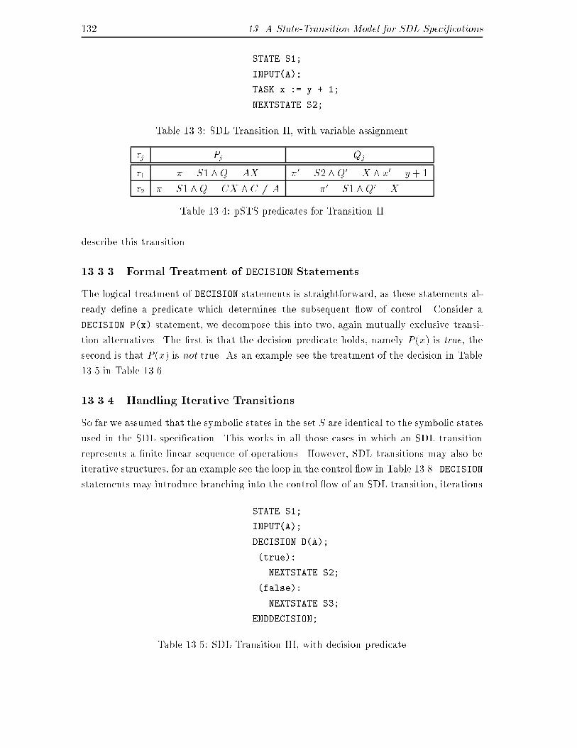
132 13. A State-Transition Model for SDL Speci�cationsSTATE S1;INPUT(A);TASK x := y + 1;NEXTSTATE S2;Table 13.3: SDL Transition II, with variable assignment�j Pj Qj�1 � = S1 ^Q = AX �0 = S2^ Q0 = X ^ x0 = y + 1�2 � = S1 ^Q = CX ^ C 6= A �0 = S1 ^Q0 = XTable 13.4: pSTS predicates for Transition IIdescribe this transition.13.3.3 Formal Treatment of DECISION StatementsThe logical treatment of DECISION statements is straightforward, as these statements al-ready de�ne a predicate which determines the subsequent ow of control. Consider aDECISION P(x) statement, we decompose this into two, again mutually exclusive transi-tion alternatives. The �rst is that the decision predicate holds, namely P (x) is true, thesecond is that P (x) is not true. As an example see the treatment of the decision in Table13.5 in Table 13.6.13.3.4 Handling Iterative TransitionsSo far we assumed that the symbolic states in the set S are identical to the symbolic statesused in the SDL speci�cation. This works in all those cases in which an SDL transitionrepresents a �nite linear sequence of operations. However, SDL transitions may also beiterative structures, for an example see the loop in the control ow in Table 13.8. DECISIONstatements may introduce branching into the control ow of an SDL transition, iterationsSTATE S1;INPUT(A);DECISION D(A);(true):NEXTSTATE S2;(false):NEXTSTATE S3;ENDDECISION;Table 13.5: SDL Transition III, with decision predicate

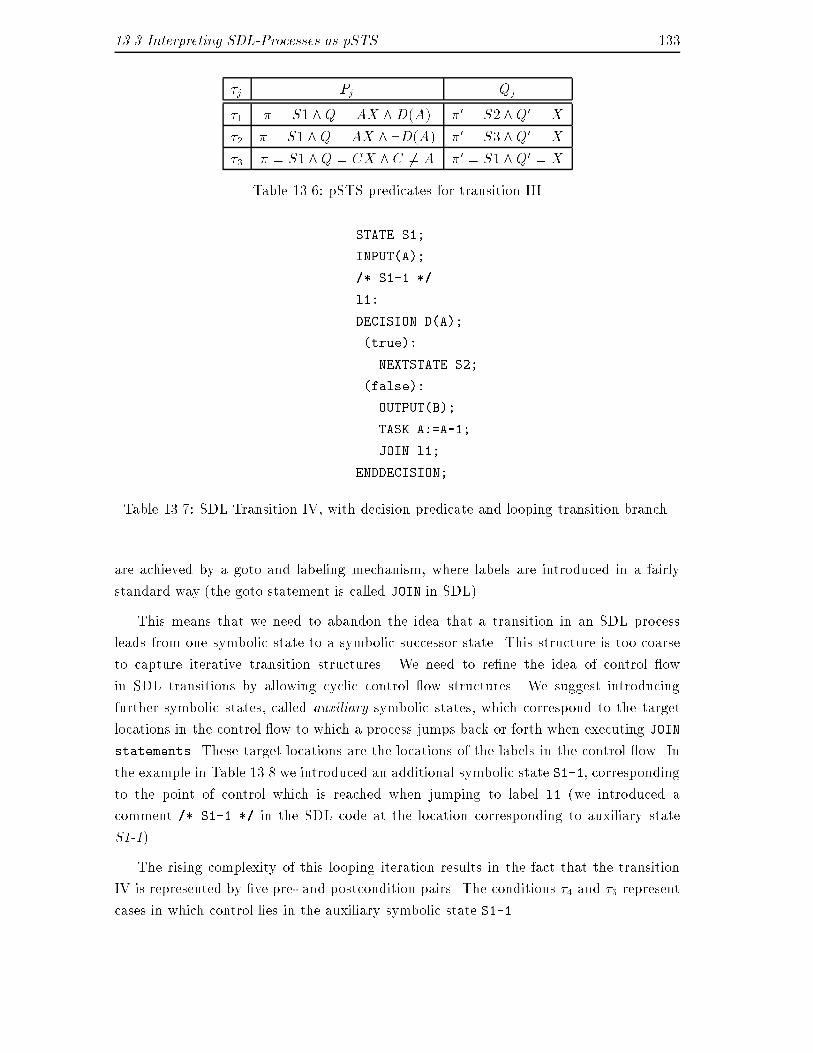
13.3 Interpreting SDL-Processes as pSTS 133�j Pj Qj�1 � = S1^Q = AX ^D(A) �0 = S2^Q0 = X�2 � = S1 ^Q = AX ^ :D(A) �0 = S3^Q0 = X�3 � = S1^Q = CX ^ C 6= A �0 = S1^Q0 = XTable 13.6: pSTS predicates for transition IIISTATE S1;INPUT(A);/* S1-1 */l1:DECISION D(A);(true):NEXTSTATE S2;(false):OUTPUT(B);TASK A:=A-1;JOIN l1;ENDDECISION;Table 13.7: SDL Transition IV, with decision predicate and looping transition branch.are achieved by a goto and labeling mechanism, where labels are introduced in a fairlystandard way (the goto statement is called JOIN in SDL).This means that we need to abandon the idea that a transition in an SDL processleads from one symbolic state to a symbolic successor state. This structure is too coarseto capture iterative transition structures. We need to re�ne the idea of control owin SDL transitions by allowing cyclic control ow structures. We suggest introducingfurther symbolic states, called auxiliary symbolic states, which correspond to the targetlocations in the control ow to which a process jumps back or forth when executing JOINstatements. These target locations are the locations of the labels in the control ow. Inthe example in Table 13.8 we introduced an additional symbolic state S1-1, correspondingto the point of control which is reached when jumping to label l1 (we introduced acomment /* S1-1 */ in the SDL code at the location corresponding to auxiliary stateS1-1).The rising complexity of this looping iteration results in the fact that the transitionIV is represented by �ve pre- and postcondition pairs. The conditions �4 and �5 representcases in which control lies in the auxiliary symbolic state S1-1.

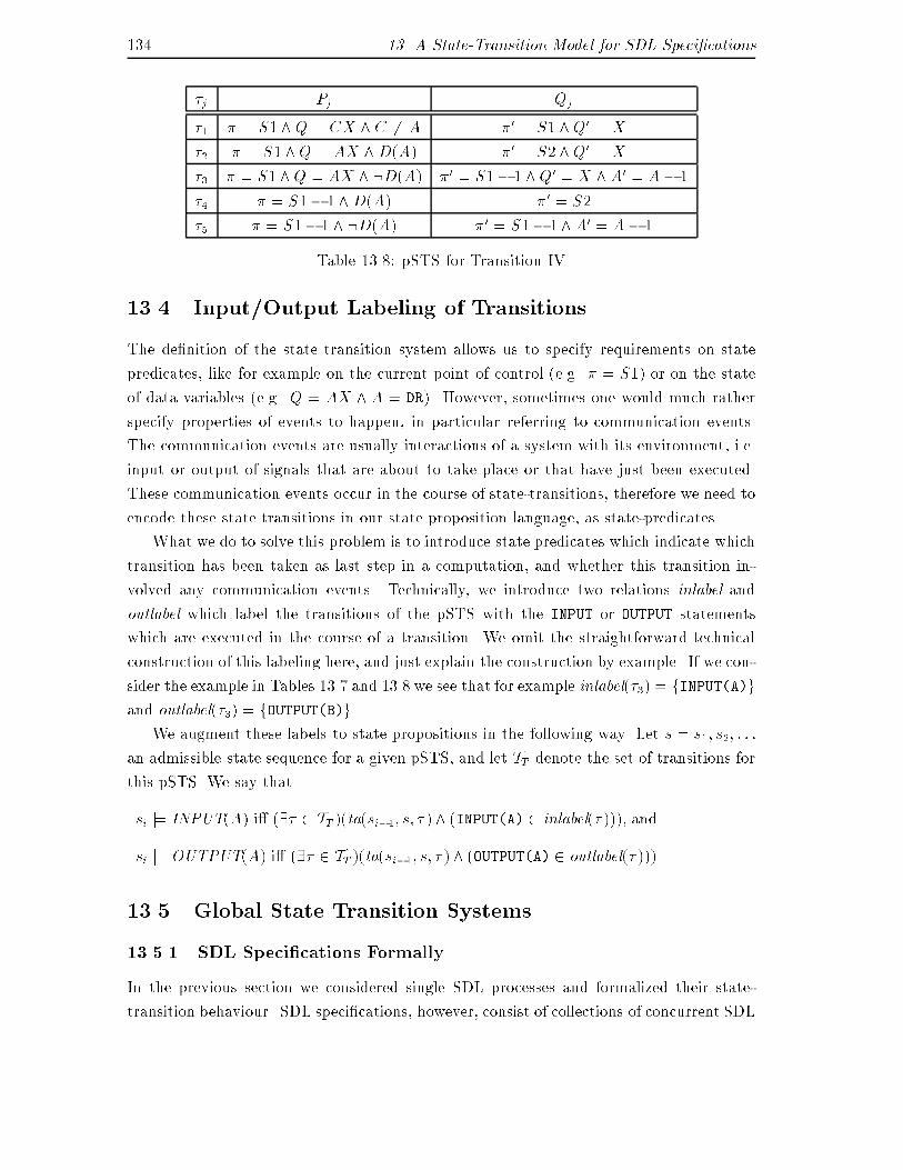
134 13. A State-Transition Model for SDL Speci�cations�j Pj Qj�1 � = S1^ Q = CX ^ C 6= A �0 = S1^Q0 = X�2 � = S1^Q = AX ^D(A) �0 = S2^Q0 = X�3 � = S1^Q = AX ^ :D(A) �0 = S1� 1 ^Q0 = X ^ A0 = A� 1�4 � = S1� 1^D(A) �0 = S2�5 � = S1� 1 ^ :D(A) �0 = S1� 1 ^A0 = A� 1Table 13.8: pSTS for Transition IV13.4 Input/Output Labeling of TransitionsThe de�nition of the state transition system allows us to specify requirements on statepredicates, like for example on the current point of control (e.g. � = S1) or on the stateof data variables (e.g. Q = AX ^ A = DR). However, sometimes one would much ratherspecify properties of events to happen, in particular referring to communication events.The communication events are usually interactions of a system with its environment, i.e.input or output of signals that are about to take place or that have just been executed.These communication events occur in the course of state-transitions, therefore we need toencode these state transitions in our state proposition language, as state-predicates.What we do to solve this problem is to introduce state predicates which indicate whichtransition has been taken as last step in a computation, and whether this transition in-volved any communication events. Technically, we introduce two relations inlabel andoutlabel which label the transitions of the pSTS with the INPUT or OUTPUT statementswhich are executed in the course of a transition. We omit the straightforward technicalconstruction of this labeling here, and just explain the construction by example. If we con-sider the example in Tables 13.7 and 13.8 we see that for example inlabel(�3) = fINPUT(A)gand outlabel(�3) = fOUTPUT(B)g.We augment these labels to state propositions in the following way. Let s = s1; s2; : : :an admissible state sequence for a given pSTS, and let TT denote the set of transitions forthis pSTS. We say thatsi j= INPUT(A) i� (9� 2 TT )(ta(si�1; s; �)^ (INPUT(A) 2 inlabel(�))), andsi j= OUTPUT(A) i� (9� 2 TT )(ta(si�1; s; �)^ (OUTPUT(A) 2 outlabel(�))).13.5 Global State Transition Systems13.5.1 SDL Speci�cations FormallyIn the previous section we considered single SDL processes and formalized their state-transition behaviour. SDL speci�cations, however, consist of collections of concurrent SDL

13.5 Global State Transition Systems 135processes. We say that the Global State Transition System (GSTS) GP corresponding toan SDL speci�cation P is a tuple GP = (P 0; : : : ; Pn) where each P i for i = 1; : : : ; n is apSTS. P 0 represents the environment. P 0 (which represents the environment behaviour)is not a full pSTS, it only consists of an input and an output alphabet, and an inputqueue. P 0 has no state and we rely on the facilitating assumption that P 0 will provideany of the other processes with input signals whenever these wish to consume any suchsignal, and that P 0 consumes instantly any signal which it receives from any process ofthe SDL system.13.5.2 Formal Treatment of Communication in SDL Speci�cationsSDL processes communicate asynchronously via in�nite queues. There is one input queueper SDL process. For an SDL speci�cation we interpret the sending of a signal A from aprocess P 1 to a process P 2, indicated by an OUTPUT(A) statement, such that a signal oftype A is appended to P 2's input queue Q2. We slightly simplify the SDL mechanism ofmapping of an output signal to a receiving process by assuming that a signal A is sent froma process P i to a process P j i� A 2 Ij7. Furthermore, we require (8i = 1; : : : ; n)(8a 2Oi)(9j 6= i)(a 2 Ij) and (8i = 1; : : : ; n)(Oi \ I i = ;). As we saw in Section 13.3, theexecution of an INPUT(A) statement (which in the SDL terminology is often just referredto as signal-consumption) represents an action purely local to an SDL process, and wehave given the semantic interpretation there.Transition Predicates for OUTPUT statements. The execution of an OUTPUTstatement involves a non-local action. It means that the execution of the statement isa local event to the sending process, whereas the reception (which in SDL is di�erent fromthe consumption of the message and just means that the message will be appended to thetail of the receiving process' input queue) is a local event of another (the receiving) process.Therefore, one can not formalize these transitions by state propositions that solely refer tostate variable of only one process. Table 13.10 presents a simple example of a two-processSDL speci�cation P = (P 0; P 1; P 2). Transition �11 describes both the state change in P 1and the appending of the signal B to the input queue of P 2. Although strictly speakingthis transition also changes the state of process P 2 for our formal treatment we considertransition �11 to be a transition belonging to process P 1.13.5.3 Global System States and TransitionsLet GP = (P 0; : : : ; Pn) denote the GSTS for an SDL speci�cation P . We say that thevector s = (s1; : : : ; sn) is a global system state (GSS) of the SDL speci�cation P i� si is a7In SDL this involves a mapping of signal names via signal lists to signal routes which point to thereceiving process.

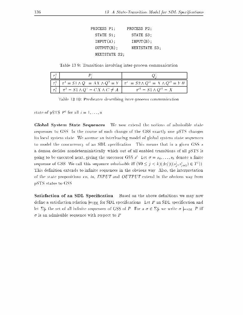
136 13. A State-Transition Model for SDL Speci�cationsPROCESS P1; PROCESS P2;STATE S1; STATE S3;INPUT(A); INPUT(B);OUTPUT(B); NEXTSTATE S3;NEXTSTATE S2;Table 13.9: Transitions involving inter-process communication�1j P 1j Q1j�11 �1 = S1^Q1 = AX ^Q2 = Y �01 = S2^ Q01 = X ^Q02 = Y B�12 �1 = S1 ^Q1 = CX ^ C 6= A �01 = S1 ^Q01 = XTable 13.10: Predicates describing inter-process communicationstate of pSTS P i for all i = 1; : : : ; n.Global System State Sequences. We now extend the notions of admissible statesequences to GSS. In the course of each change of the GSS exactly one pSTS changesits local system state. We assume an interleaving model of global system state sequencesto model the concurrency of an SDL speci�cation. This means that in a given GSS sa demon decides nondeterministically which out of all enabled transitions of all pSTS isgoing to be executed next, giving the successor GSS s0. Let � = s0; : : : ; sk denote a �nitesequence of GSS. We call this sequence admissible i� (80 � j < k)(9� il )((sij; sij+1) 2 T i)).This de�nition extends to in�nite sequences in the obvious way. Also, the interpretationof the state propositions en, ta, INPUT and OUTPUT extend in the obvious way frompSTS states to GSS.Satisfaction of an SDL Speci�cation. Based on the above de�nitions we may nowde�ne a satisfaction relation j=SDL for SDL speci�cations. Let P an SDL speci�cation andlet �!P the set of all in�nite sequences of GSS of P . For a � 2 �!P we write � j=SDL P i�� is an admissible sequence with respect to P .

Chapter 14Using Temporal Logic for SDLSpeci�cationsMany authors have advocated the use of temporal logics for high level speci�cation ofabstract requirements on communication protocols and services (see for example [148] and[61, 62]). The characterisation of properties by the use of temporal logic is accomplishedby interpreting the temporal logic speci�cation as a �lter on the set of all state sequences,resulting in a set of admissible state sequences.Now, as we have seen in Chapter 13, SDL speci�cations also specify admissible se-quences of states. But, as we have noted before, not all desirable properties are expressiblein SDL, as for example liveness properties and hard real-time bounds. What we suggestnow is to use a combination SDL and temporal logic speci�cations, where the tempo-ral logic speci�cation acts as a �lter on the admissible sequences described by an SDLspeci�cation. We call these combined speci�cations complementary speci�cations.When using this speci�cation approach a crucial point is the selection of a suitabletemporal logic language. For an overview over temporal logics we refer to [52]. In theremainder we will use a temporal logics similar to the logic described in [113], calledPropositional Temporal Logic (PTL), and extensions based on PTL. However, it shouldbe fairly easy to translate formulas into other temporal logic frameworks, for example intothe Temporal Logic of Actions (TLA) [101], or into branching time temporal logics [52].A State Proposition Language. When using complementary QoS speci�cations weneed to identify a set of state propositions which we may use in the temporal logic formulas.When determining the set of state propositions one also determines which part of thestate information is observable1. We will not treat this question in depth here. Thedetermination of the visible state component is mainly dependent upon the particular1This corresponds to the determination of the sets �(�) in [14].

138 14. Using Temporal Logic for SDL Speci�cationsspeci�cation problem considered. We assume that the state propositions we use all referto observable components of the system state, and we use in particular the following statepropositions for an SDL speci�cation P :� Actual State: let S = Si1; : : : ; Sin denote the symbolic states for a given process P iof P , then at Sik denotes the state proposition that the i-th component of the globalsystem state is in symbolic state Sik, i.e. �i = Sik.� Input and output: we use the state propositions INPUT and OUTPUT as de�nedabove to denote that we are in a state where an input or an output of a signal hasjust occurred in the last GSS transition.� Data: we allow the reference to visible data variables and allow standard comparisonoperators on the variables. However, we require that the resulting expressions remainstate propositions.We allow state formulas to be constructed by using boolean operators between state propo-sitions.Example. The state formula n � 3 ^ INPUT(A) holds in all GSS in which the valueof variable n is less than or equal to 3 and an input of a signal of type A has just beenexecuted. The state formula at S1 � n � 3 holds in all those GSS in which if the controlis in symbolic state S1 then the value of variable n is greater than or equal to 3.14.1 Propositional Temporal LogicThe Propositional Temporal Logic (PTL) we use here is a linear time temporal logic takenfrom [113]. For a formalization of the syntax and semantics of PTL we refer the readerto [113]. Let p denote a state predicate. This means that p is constructed from statepropositions. We say that the formula 3p holds in a state s i� p holds in s or in somefuture state. In addition to the standard operators of PTL as de�ned in [113] we de�ne astrong eventuality operator 3: so that 3: p holds in some future state s2. The formula 2p,which denotes a syntactic abbreviation for :3:p, holds in a state s i� p holds in s and inevery successor state of s. Temporal Logic includes the propositional calculus. The formalsemantics of PTL de�ne a satisfaction relation j=PTL. An execution sequence � = s0; : : :of states si satis�es a formula � i� � holds in s0, and we write � j=PTL �. We say that asystem satis�es a formula � i� all its execution sequences satisfy �.2The formal de�nition of the semantics of this operator is si j= 3: p i� (9j > i)(sj j= p).

14.2 Metric Temporal Logic 13914.2 Metric Temporal LogicReal-Time extended temporal logic has been suggested in various places as a suitable toolfor the speci�cation of real-time systems (see for example [67], [1], [87] and [124]). Weapply a variant of these logics called metrical temporal logic (MTL) to the speci�cationof QoS requirements3. The language of Propositional Temporal Logic (PTL) is a propersyntactic subset of MTL.Timed Observation Sequences. The models over which we interpret PTL formulasare timed observation sequences o = o1; : : : (see [14]). Each oi corresponds to a pair si; Iiwhere si is a state and Ii is a numeric interval expression. Let li and ri denote the leftand right boundaries of the Interval Ii, then for example the timed observation (si; [li; ri[)means that state si can be observed in the interval starting with li and ending with,but not including, ri. As we only consider instantaneous state changes the sequence ofintervals II can be replaced by single time stamps, for example for an interval Ii alwaysby the left interval boundary li. We assume sequences li to be monotonic. We assume�nite precision of our clocks, i.e. we assume that every state change coincides with a clickof the clock from which we derive the timed observation. Therefore the set of naturalnumbers N su�ces as domain for the interval expressions [14]. We use MTL to specifyproperties of concurrent systems based on an interleaving interpretation of concurrent statetransitions. Assume that s1; s2 and s3 are GSS of an SDL speci�cation. Furthermore, letboth s1; s2; s3; : : : and s1; s3; s2; : : : be admissible sequences in the untimed model. If wenow want to express that both s2 and s3 may occur at the same time (which means thatthey have the same time stamp) in any order we have to allow that both timed observationsequence (s1; l1) ! (s2; l2) ! (s3; l3) ! : : : and (s1; l1) ! (s3; l2) ! (s2; l3) ! : : : areadmissible and that l2 = l3. Hence in this interleaving model we assume the sequence lito be weakly-monotonic [14].MTL language and semantics. MTL contains formulas of the form 3I� which assertthat one of the following states within the time-interval described by expression I is astate which satis�es �. Formulas of the form 2I� assert that all states in the time-intervaldescribed by I satisfy �. The expression I describes an either open or closed intervalover the time domain and we sometimes use semi-algebraic expressions to refer to theseintervals. As an example the formula2�5(:OUTPUT(A))3Our introduction will be rather informal and we will not present all possible operators, we restrictourselves to a minimal subset of the language which we need to carry out our example. For a completeformal de�nition of the syntax and semantics of MTL we refer the reader to [14] and [67, chapter 3.4]

140 14. Using Temporal Logic for SDL Speci�cationsexpresses the property that in all subsequent system states i in which the time stampTi is less than or equal to 5 the state proposition OUTPUT(A) is false. In analogy tothe satisfaction relation for PTL we write o j=MTL p i� the sequence o satis�es the MTLformula p.14.3 Complementary Speci�cationsAssume we have an SDL speci�cation P and a set of formulas M in MTL. Now, P andM are complementary speci�cations if we require from the speci�ed system that for all itstimed observation sequences o = (s0; t0); : : : the following condition holds:s j=SDL P ^ o j=MTL M:4Example. Let us consider the INRES connection establishment example in Figure 12.1again. The SDL speci�cation describes a sequence of possible executions. We will usecomplementary speci�cations to specify an interesting liveness property and a boundedresponse hard real-time constraint.First we will look at liveness. It is important to require that the system is live, namelythat when a request for a connection establishment has been issued by sending a CRmessage, then eventually the process Initiator will eventually receive either a CC or aDR signal, or it will eventually issue a IDISind signal to the service user to indicate that aconnection establishment was not possible. Liveness properties are not expressed by SDLspeci�cations, so this requirement can be expressed by the following complementary PTLformula:2(OUTPUT(CR) � 3(INPUT(CC)_ INPUT(DR)_ OUTPUT(IDISind))):Now, as we argued in Chapter 12.1, it is important to know that any of these responsesto the sending of the CR signal happens within a reasonable period of time, say within ttime units. In the SDL speci�cation the timer T has been used to require this, but we haveargued above why the usage of the timer in this context cannot guarantee this conditionto hold. Therefore we transform the above liveness requirement into a real-time boundedresponse requirement which we specify using MTL in the following way:2(OUTPUT(CR) � 3�t(INPUT(CC)_ INPUT(DR)_ OUTPUT(IDISind))):14.4 Using PTL and MTL for MSC speci�cationsIn Section 7.6 we explained how GSTGs derived from MSC speci�cations relate to Manna-Pnueli Basic Transition Systems and how PTL can be used to specify liveness properties4Note that PTL is a syntactic subset of MTL and hence included in this de�nition.

14.4 Using PTL and MTL for MSC speci�cations 141for MSCs. The state propositions we use as basic propositions for PTL formulas are thepredicates en(�) and ta(�) where � is a transition in the GSTG. In a similar way like forSDL speci�cations we would like to make assertions not only on these state predicates,but also using propositions referring to communication events.It is therefore necessary to use a similar labeling technique like for the transitions inan SDL speci�cation. We label transitions with the names of the communication eventswhich cause the transition to happen, so in the GSTG in Figure 7.1 the transition fromS1 to S2 is labeled by y. It should be noted that for example the state proposition ta(y)holds in several di�erent states (S2 and S4), namely all those states that can be enteredby executing a y event. If the transition y represents a send (receive) event of a messageof type a, then we sometimes use the event types as state propositions, e.g. we write !a,instead of ta(y), and ?a instead of ta(z).Example. If we were for example to require that in our example a send event willeventually be followed by a receive event, which is a liveness requirement that preventsthe system from looping on state S2 forever, we would write in PTL2(!a � 3?a):The interpretation of MTL formulas over models generated by MSC speci�cations is astraightforward extension of the interpretation of the formulas over SDL speci�cations.

Chapter 15Specifying QoS: DelaysFigure 15.1 presents the example of a simple Sender/Receiver Service (SRS) speci�ed usingMSCs. The example works as follows. A user U1 of the service requests the transmissionof some data by sending a UDreq signal to the sender process S which in turn requests thetransmission of the data from a medium service M by sending a MDreq. The medium serviceis unreliable. However, in case the transmission is successful the medium service will deliverthe data to the receiver process R by means of an MDind message, and the receiver deliversthe data to the user process U2. Although the medium service is unreliable we neverthelessassume that it is capable of reliably indicating to the sender process by means of an MDconsignal whether the data has been delivered successfully to the receiver process, or by anMDrej that this is not the case. Successful delivery will be indicated to the service user U1by an UDcon signal, and unsuccessful delivery by an UDrej signal.The example does not re ect any particular real-world telecommunications service,however as pointed out in [103] some Asynchronous Transfer Mode (ATM) adaptationlayer service will have to implement a similar functionality as the medium service in theSRS example. The SDL speci�cation presented in Figure 15.2 presents a similar service.However, in the SDL speci�cation we focus on the speci�cation of the behaviour of thesender S and receiver R processes and omit a speci�cation of the behaviour of processesU1, M and U2.Related work. For an overview on specifying real-time constraints using MTL we referthe reader to [14]. [51] describes aspects of the JVTOS service using MSCs, and describesQoS measurements in TLA [101]. It has been suggested to attribute MSCs with timinginformation, and [117] investigates how timing constraints attached to MSCs can be veri-�ed using the Dechter, Meiri and Pearl algorithm. This work relies on timing informationrequiring earliest and latest occurrence of one event on the occurrence of another event.

144 15. Specifying QoS: DelaysC1

C2

U1 S M R U2

U1 S M R U2

C2

C1

U1 S M R U2

C2

C1

MDconMDind

UDrej

UDreqMDreq

UDcon

MDrej

UDind

Figure 15.1: MSC Speci�cation of SRS example.UDind

MDind

UDcon

MDconMDrejMDreq

S1

UDrej

UDreq

S2

S1

S2

S1

S1

S2

PROCESS S PROCESS R

Figure 15.2: SDL Speci�cation of SRS example.

15.1 Delay bounds on SRS 14515.1 Delay bounds on SRSWe now discuss a few potential delay bounds on the SRS service and specify them usingcomplementary MSC and PTL speci�cations. The speci�cations given here are inteded todemonstrate the applicability of the approach in principle.15.1.1 Service Response Delay BoundSimilar to what we discussed in the context of the INRES example an important livenessrequirement for the SRS service is that if the service process has received a UDreq it willeventually indicate either an UDcon or a UDrej signal to the service user in order to indicatesuccessful or unsuccessful delivery of data. We describe this requirement by2(!UDreq � 3(?UDcon_?UDrej)):However, many real-time applications may require an indication to be given within a real-time bound of for example t1 time units, which is expressed by the following boundedresponse requirement: 2(!UDreq � 3�t1(?UDcon_?UDrej)):15.1.2 Service Processing Delay BoundThe sender process S may need some time to process the user data before sending outa MDreq to request data transmission from the medium service. The service processingdelay bound requirement reads2(?UDreq � 3�t2!MDreq):15.1.3 Message Transmission Delay Bound at Service InterfaceDepending on the communication mechanism used at the service interface between pro-cesses S and M the transmission of a message between both may consume time. In orderto limit the transmission time to at most t3 time units we write2(!MDreq � 3�t3?MDreq):15.1.4 Medium Transmission Delay BoundThe process M is an abstraction for the whole communication subsystems which we use inorder to transfer the data. One may wish to constrain the time between the events of thereception of the MDreq signal and the output of the MDind signal to t4 time units, but onlyif the transmission is successful.2((?MDreq^3!MDind) � 3�t4!MDind)

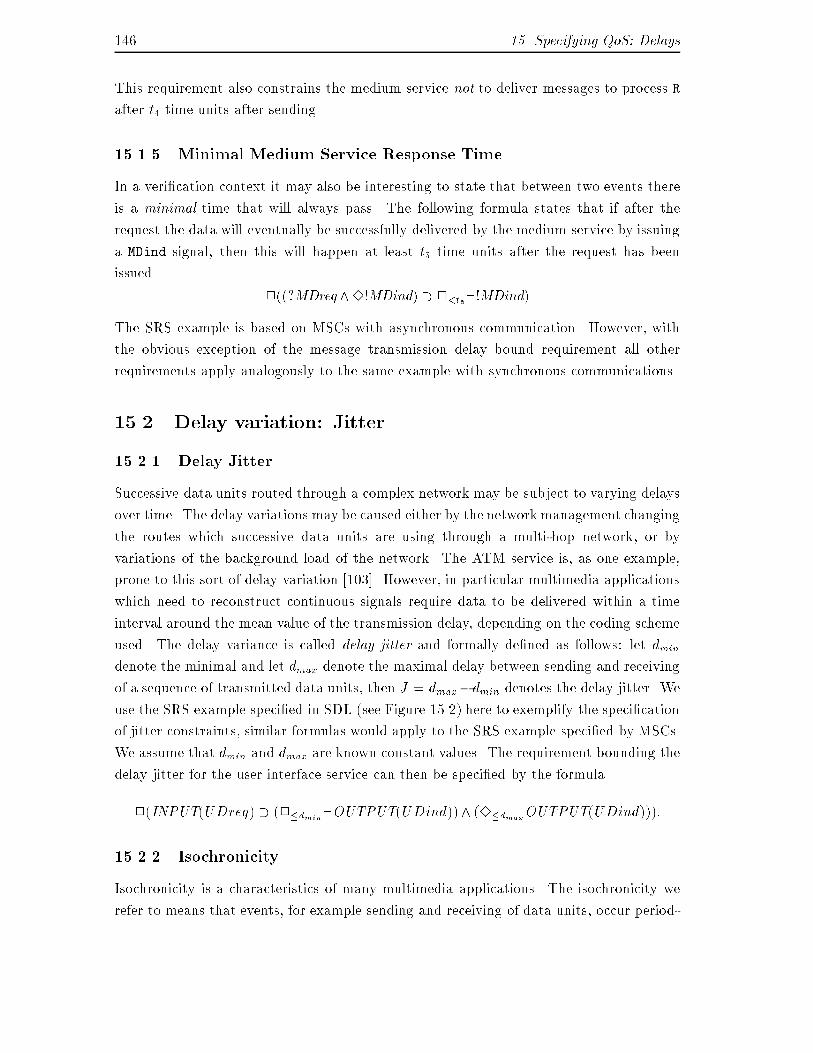
146 15. Specifying QoS: DelaysThis requirement also constrains the medium service not to deliver messages to process Rafter t4 time units after sending.15.1.5 Minimal Medium Service Response TimeIn a veri�cation context it may also be interesting to state that between two events thereis a minimal time that will always pass. The following formula states that if after therequest the data will eventually be successfully delivered by the medium service by issuinga MDind signal, then this will happen at least t5 time units after the request has beenissued. 2((?MDreq^3!MDind) � 2<t5:!MDind)The SRS example is based on MSCs with asynchronous communication. However, withthe obvious exception of the message transmission delay bound requirement all otherrequirements apply analogously to the same example with synchronous communications.15.2 Delay variation: Jitter15.2.1 Delay JitterSuccessive data units routed through a complex network may be subject to varying delaysover time. The delay variations may be caused either by the network management changingthe routes which successive data units are using through a multi-hop network, or byvariations of the background load of the network. The ATM service is, as one example,prone to this sort of delay variation [103]. However, in particular multimedia applicationswhich need to reconstruct continuous signals require data to be delivered within a timeinterval around the mean value of the transmission delay, depending on the coding schemeused. The delay variance is called delay jitter and formally de�ned as follows: let dmindenote the minimal and let dmax denote the maximal delay between sending and receivingof a sequence of transmitted data units, then J = dmax�dmin denotes the delay jitter. Weuse the SRS example speci�ed in SDL (see Figure 15.2) here to exemplify the speci�cationof jitter constraints, similar formulas would apply to the SRS example speci�ed by MSCs.We assume that dmin and dmax are known constant values. The requirement bounding thedelay jitter for the user interface service can then be speci�ed by the formula2(INPUT(UDreq) � (2�dmin:OUTPUT(UDind))^ (3�dmaxOUTPUT(UDind))):15.2.2 IsochronicityIsochronicity is a characteristics of many multimedia applications. The isochronicity werefer to means that events, for example sending and receiving of data units, occur period-

15.2 Delay variation: Jitter 147ically at equally distanced points of time. Again, the example formulas given here refer tothe SDL speci�cation of the SRS example.Isochronous sending and receiving. Isochronous sending is a characteristic of a traf-�c source. It is a characteristical requirement on simple coding schemes for audio orvideo data where samples of the analogous signal are taken and sent periodically. Thecharacterization of isochronous sending reads2(INPUT(UDreq) � (:3: <tINPUT(UDreq)^3=tINPUT(UDreq))):On the receiving side the receiver may require to have successive data units availableat isochronous moments in time. This may be expressed in a way very similar to theisochronous send characterization, namely as2(INPUT(UDind) � (:3: <tINPUT(UDind)^3=tINPUT(UDind))):15.2.3 RatesRates like throughput are usually measured by the number of data units processed pertime period. The temporal logic we have proposed so far does not permit the countingof events. Event counting requires a non-trivial extension of the logic1. However, it maybe useful to specify that the time interval in between two events of some particular type,e.g. the sending of events, is restricted to a time span t. This is a reciprocal considerationcompared to the number of events per time unit based rate speci�cation. For example, inorder to specify a constraint on the output rate of the medium service used in the SRSexample we may require that the time between two successive MDind events is limited tobe less than or equal to t6.2(OUTPUT(MDind) � 3: �t6OUTPUT(MDind)):It is more appropriate to call this requirement the bounded inter-send time requirementinstead of calling it a throughput requirement because throughput may be achieved bysmall inter-send times for a while, followed by a period of silence. This is not captured bythe requirement presented here.1For an example of how to incorporate event counting in Temporal Logics see [61, 62].

Chapter 16Specifying QoS-mechanismsIn this Chapter we show a method for the speci�cation of QoS mechanisms based on thecomplementary use of SDL and MSC speci�cations and temporal logic formulas. The QoSmechanisms we refer to are QoS negotiation, reaction on QoS guarantee violation, anddelay jitter compensation.16.1 QoS NegotiationFigure 16.1 describes a QoS negotiation scenario. Assume that this speci�cation is some-how related to the speci�cation of the SRS example in Figure 15.11. The functioning ofthe negotiation is quite obvious. The user U1 requests an increase in bandwidth by send-ing a UINCreq signal which the service forwards to the medium (MINCreq) (it is assumedthat there it is processed by the appropriate network management process). The mediumeither grants the increase (MINCcon) or it refuses the increase (MINCrej). Both reactionsare indicated accordingly to the user. The following formula limits the constraining im-pact of the response time requirement on the medium service by only requiring the QoSguarantee to be satis�ed if the QoS level has been granted (by the medium issuing theMINCcon signal).2(!MINCcon � 2((?MDreq^3!MDind) � 3�t4!MDind)))16.2 Reaction on QoS Violation.It may be useful to specify a reaction on the violation of QoS requirement without requiringthat the violation invalidates the behaviour against the system speci�cation. Let us lookat the SRS example again and let us assume that we monitor the response time behaviour1The example has been inspired by an example of QoS negotiation in the context of ATM based virtualprivate networks given in [58].

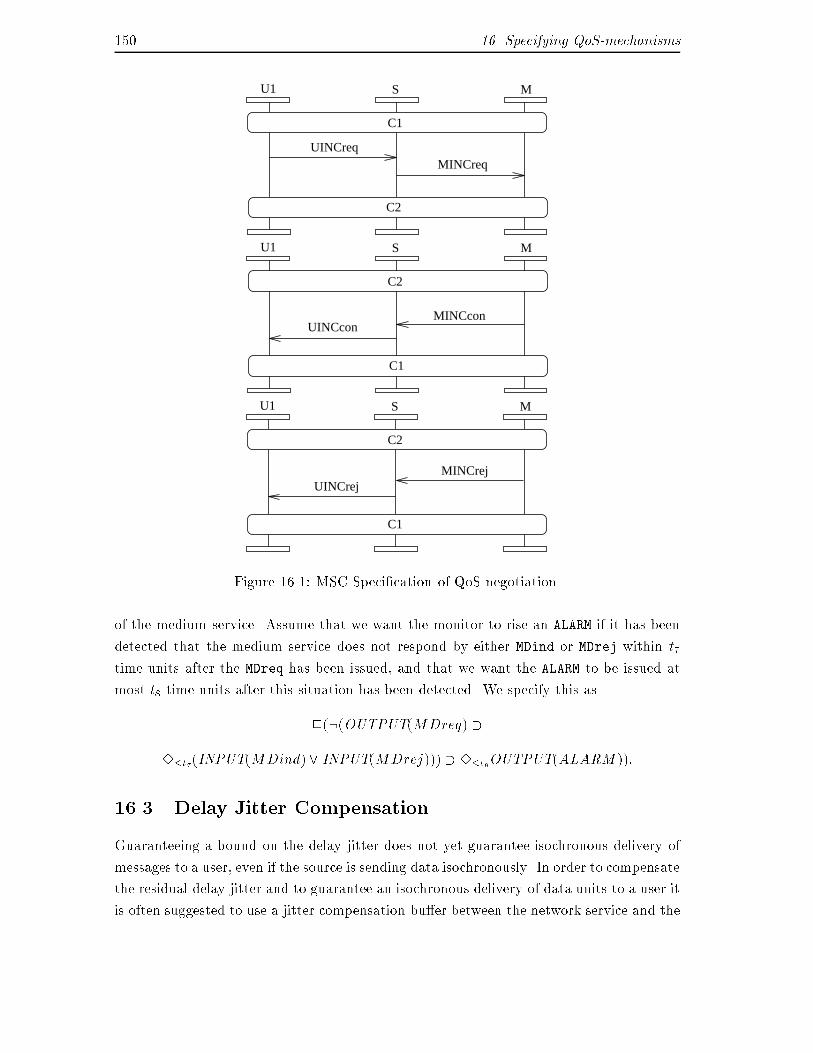
150 16. Specifying QoS-mechanismsS

MINCconUINCcon

MU1

C1

C2

S M

MINCrejUINCrej

C2

C1

U1

S M

UINCreqMINCreq

C1

C2

U1

Figure 16.1: MSC Speci�cation of QoS negotiation.of the medium service. Assume that we want the monitor to rise an ALARM if it has beendetected that the medium service does not respond by either MDind or MDrej within t7time units after the MDreq has been issued, and that we want the ALARM to be issued atmost t8 time units after this situation has been detected. We specify this as2(:(OUTPUT(MDreq) �3�t7(INPUT(MDind) _ INPUT(MDrej))) � 3�t8OUTPUT(ALARM)):16.3 Delay Jitter CompensationGuaranteeing a bound on the delay jitter does not yet guarantee isochronous delivery ofmessages to a user, even if the source is sending data isochronously. In order to compensatethe residual delay jitter and to guarantee an isochronous delivery of data units to a user itis often suggested to use a jitter compensation bu�er between the network service and the

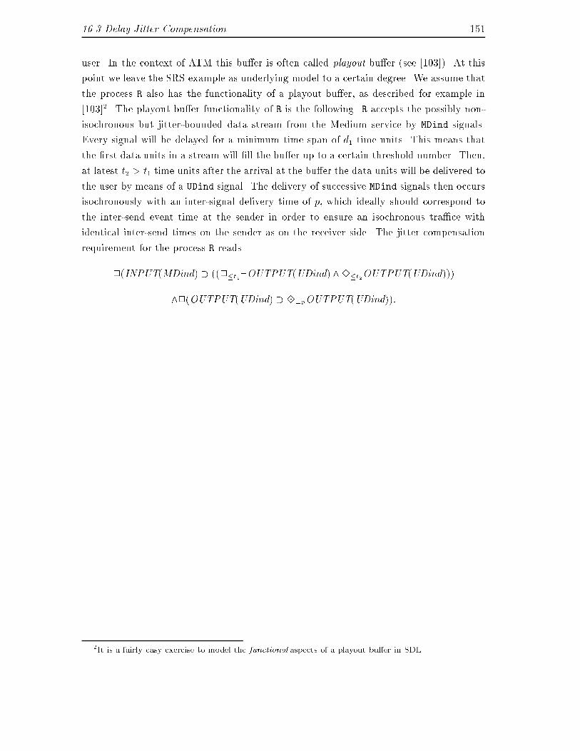
16.3 Delay Jitter Compensation 151user. In the context of ATM this bu�er is often called playout bu�er (see [103]). At thispoint we leave the SRS example as underlying model to a certain degree. We assume thatthe process R also has the functionality of a playout bu�er, as described for example in[103]2. The playout bu�er functionality of R is the following. R accepts the possibly non-isochronous but jitter-bounded data stream from the Medium service by MDind signals.Every signal will be delayed for a minimum time span of d1 time units. This means thatthe �rst data units in a stream will �ll the bu�er up to a certain threshold number. Then,at latest t2 > t1 time units after the arrival at the bu�er the data units will be delivered tothe user by means of a UDind signal. The delivery of successive MDind signals then occursisochronously with an inter-signal delivery time of p, which ideally should correspond tothe inter-send event time at the sender in order to ensure an isochronous tra�ce withidentical inter-send times on the sender as on the receiver side. The jitter compensationrequirement for the process R reads2(INPUT(MDind) � ((2�t1:OUTPUT(UDind) ^3�t2OUTPUT(UDind)))^2(OUTPUT(UDind) � 3: =pOUTPUT(UDind)):

2It is a fairly easy exercise to model the functional aspects of a playout bu�er in SDL.

Chapter 17DiscussionWe will discuss some problems arising from the use of complementary speci�cations inthe context of quality of service speci�cations. First, we discuss the relation of systemperformance and quality of service. We address the speci�cation of the characteristics of alower layer communication system, a communication mechanism, and how this relates tothe QoS characteristics o�ered to a higher layer user. This leads to a veri�cation problem,and we discuss which veri�cation methods can be applied.17.1 System Performance to QoS MappingA communications system generally o�ers a service to a higher-layer user, and usually usesa lower layer communications infrastructure. We will now investigate the question how theQoS requirements which the higher layer user imposes on the system, the communicationmechanisms inside the communications system, and �nally the QoS requirements on thelower layer communications infrastructure are interrelated. To make the terminologyless ambiguous we call the requirements of the upper layer application on the serviceQoS requirements, and the description of the properties of the underlying communicationinfrastructure system performance (a similar terminology is used in [82]).Assume that we are given a speci�cation P of the system performance, speci�cation Sof the service or the protocol which we investigate, and a speci�cation Q of the user QoSrequirements. Assume that all three speci�cations are given in terms of logic1. We nowask whether P together with S can ensure that Q can be satis�ed, or more formally:P ^ S � Q:Example. Let us consider the SRS example again, and let us assume that SRS has beentranslated into logic and is given as a speci�cation S. Furthermore, assume the system1We have shown earlier how to translate SDL speci�cations into logic descriptions.

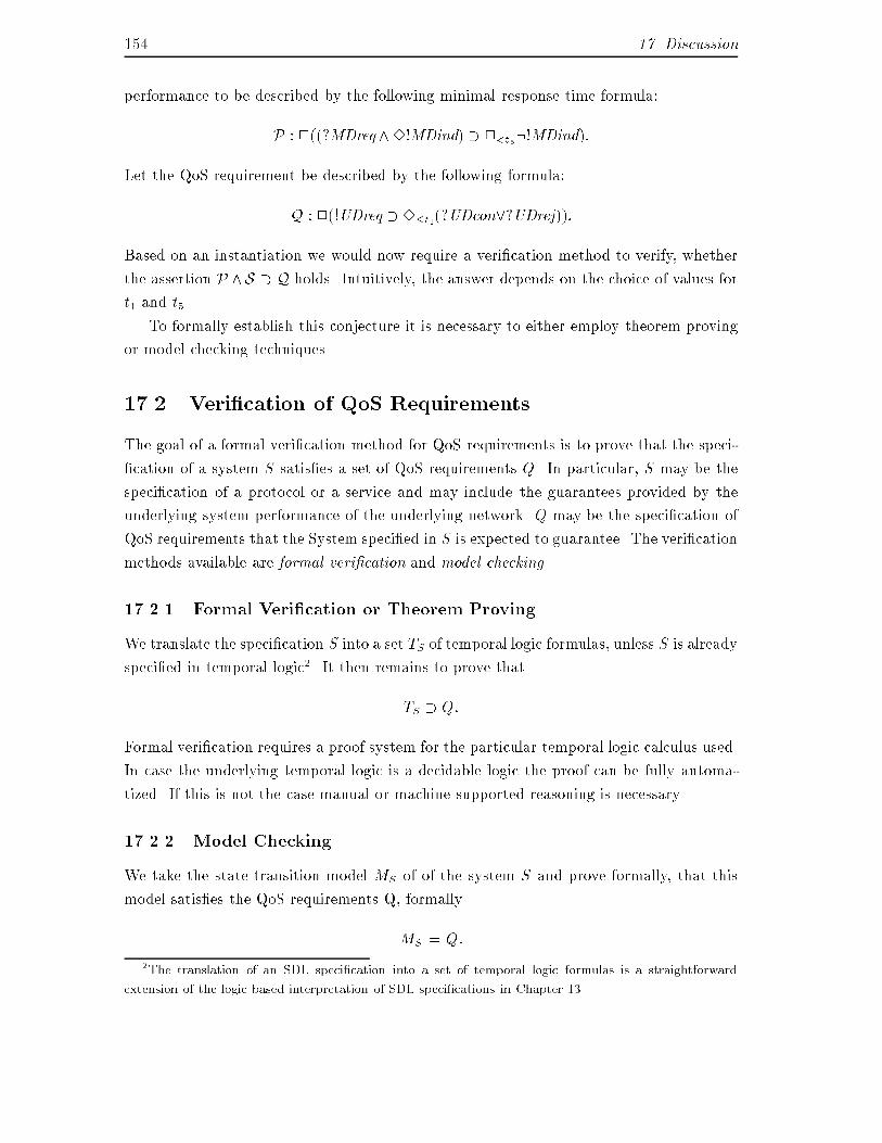
154 17. Discussionperformance to be described by the following minimal response time formula:P : 2((?MDreq^3!MDind) � 2<t5:!MDind):Let the QoS requirement be described by the following formula:Q : 2(!UDreq � 3�t1(?UDcon_?UDrej)):Based on an instantiation we would now require a veri�cation method to verify, whetherthe assertion P ^S � Q holds. Intuitively, the answer depends on the choice of values fort1 and t5.To formally establish this conjecture it is necessary to either employ theorem provingor model checking techniques.17.2 Veri�cation of QoS RequirementsThe goal of a formal veri�cation method for QoS requirements is to prove that the speci-�cation of a system S satis�es a set of QoS requirements Q. In particular, S may be thespeci�cation of a protocol or a service and may include the guarantees provided by theunderlying system performance of the underlying network. Q may be the speci�cation ofQoS requirements that the System speci�ed in S is expected to guarantee. The veri�cationmethods available are formal veri�cation and model checking.17.2.1 Formal Veri�cation or Theorem ProvingWe translate the speci�cation S into a set TS of temporal logic formulas, unless S is alreadyspeci�ed in temporal logic2. It then remains to prove thatTS � Q:Formal veri�cation requires a proof system for the particular temporal logic calculus used.In case the underlying temporal logic is a decidable logic the proof can be fully automa-tized. If this is not the case manual or machine supported reasoning is necessary.17.2.2 Model CheckingWe take the state transition model MS of of the system S and prove formally, that thismodel satis�es the QoS requirements Q, formallyMS j= Q:2The translation of an SDL speci�cation into a set of temporal logic formulas is a straightforwardextension of the logic based interpretation of SDL speci�cations in Chapter 13.

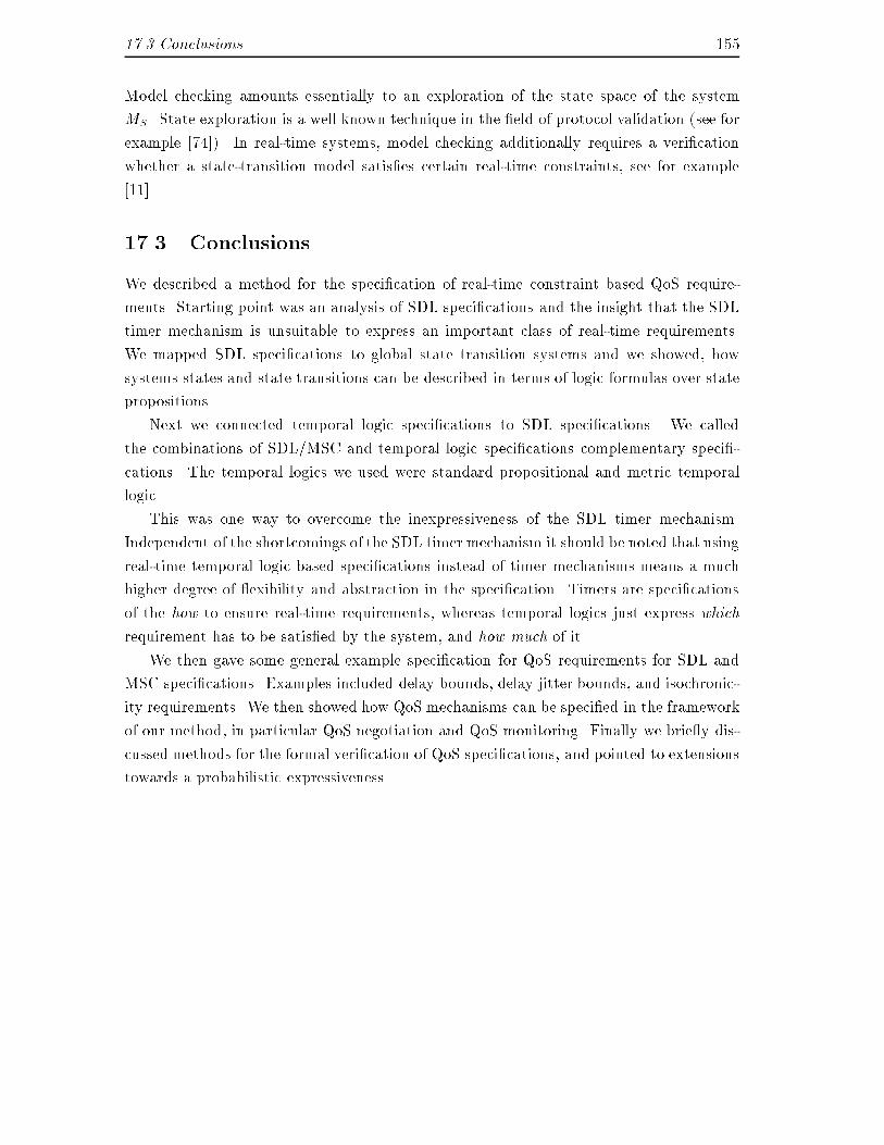
17.3 Conclusions 155Model checking amounts essentially to an exploration of the state space of the systemMS . State exploration is a well known technique in the �eld of protocol validation (see forexample [74]). In real-time systems, model checking additionally requires a veri�cationwhether a state-transition model satis�es certain real-time constraints, see for example[11].17.3 ConclusionsWe described a method for the speci�cation of real-time constraint based QoS require-ments. Starting point was an analysis of SDL speci�cations and the insight that the SDLtimer mechanism is unsuitable to express an important class of real-time requirements.We mapped SDL speci�cations to global state transition systems and we showed, howsystems states and state transitions can be described in terms of logic formulas over statepropositions.Next we connected temporal logic speci�cations to SDL speci�cations. We calledthe combinations of SDL/MSC and temporal logic speci�cations complementary speci�-cations. The temporal logics we used were standard propositional and metric temporallogic.This was one way to overcome the inexpressiveness of the SDL timer mechanism.Independent of the shortcomings of the SDL timer mechanism it should be noted that usingreal-time temporal logic based speci�cations instead of timer mechanisms means a muchhigher degree of exibility and abstraction in the speci�cation. Timers are speci�cationsof the how to ensure real-time requirements, whereas temporal logics just express whichrequirement has to be satis�ed by the system, and how much of it.We then gave some general example speci�cation for QoS requirements for SDL andMSC speci�cations. Examples included delay bounds, delay jitter bounds, and isochronic-ity requirements. We then showed how QoS mechanisms can be speci�ed in the frameworkof our method, in particular QoS negotiation and QoS monitoring. Finally we brie y dis-cussed methods for the formal veri�cation of QoS speci�cations, and pointed to extensionstowards a probabilistic expressiveness.

156 17. Discussion

Part IVE�cient Protocol Implementation

Chapter 18IntroductionIn this part of the thesis we present a method for the automatic derivation of e�cientprotocol implementations from a formal speci�cation. Optimized e�cient protocol imple-mentation has become an important issue in telecommunications systems engineering asrecently network throughput has increased much faster than computer processing power.E�ciency will be attained by two measures. First, the inherent parallelism in protocolspeci�cations will be exploited. Second, the order of execution of the operations involvedin the processing of the protocol data will be allowed to di�er from the order prescribedin the speci�cation, thus allowing operations to be executed jointly and more e�ciently.The method will be de�ned formally which is useful when implementing it as a tool.Our method starts with the SDL speci�cation of a protocol stack. We �rst derive adata- and control ow dependence graph from each SDL process. Then, in order to performcross-layer optimizations we combine the dependence graphs of di�erent SDL processes.Next, we determine the common path through the multi-layer dependence graph. Wethen parallelise this graph wherever possible which yields a relaxed dependence graph.Based on this relaxed dependence graph we interpret di�erent optimization concepts thathave been suggested in the literature, in particular the combination of data manipulationoperations. Together with these interpretations the relaxed dependence graph can beused as a foundation for a compile-time schedule on a sequential or parallel machinearchitecture.18.1 OverviewIn Figure 19.2 we present a (partial) view of the SDL speci�cation of a two layer protocolstack. It will serve as a running example in this part and we will refer to it as TLS. Thespeci�cation in Figure 19.2 is given in graphical SDL syntax (GR), Figure 19.3 contains thesame speci�cation in the textual SDL syntax (PR). We also give this textual representationto emphasize that the syntactic analysis steps we present here can be automated. A �rst

160 18. Introductionattempt towards automation of the data- and control ow analysis for SDL speci�cationshas been made in [151]. It is the purpose of our optimization and implementation methodto transform speci�cations similar to TLS into parallelised and optimized implementations.In Chapter 19 we discuss the sort of layered SDL speci�cations we consider in thispart. Here, we also argue why a direct and faithful implementation of SDL speci�cationswould lead to ine�cient implementations. This is mainly due to the structuring of SDLspeci�cations into per-layer processes and the resulting inter-layer asynchronous queuebased communication mechanism. Then we turn to a description of our analysis andoptimization method:� First, we construct a dependence graph representing control- ow and data depen-dences among statements in an SDL speci�cation. This leads us to so-called Tran-sition Dependence Graphs. Their construction is explained in Section 20.1. Forthe dependence graphs for example TLS see Figure 20.1. The dependence graphconstruction is an application of methods known from the domain of compiler op-timization and parallel compilation as they are for example described in [56] and[17]. Control ow dependences relate directly successive statements (e. g. S2 andS3 in Figure 20.1) whereas data dependences relate statements where the dependingstatement uses a variable that is de�ned in the other statement (e. g. S3 and D1 inFigure 20.1).� We optimise and parallelise operations related to processing a packet. We considerthe way the packet takes from the point where it enters the protocol stack to whereit exits. Therefore we combine transition dependence graphs belonging to di�erentSDL processes. We do so by eliminating the inter-layer communication statements,e. g. the statements S4 and S9 in the example TLS. The result is a Multi-LayerDependence graph. We describe the constructions in Chapter 21, for an example seeFigure 21.2.� Third, we identify the path a packet takes through the protocol stack in the so-called common case, from the root node representing the point where a packet isaccepted from the environment to the exit node, where the packet is conveyed tothe environment. For example, we assume that in the example TLS decision D1has one common and one uncommon branch, whereas decision D2 has two commonbranches. This resulting graph is called common path graph, for an example seeFigure 22.2. We will apply our later optimizations only to the common case part ofthe speci�cation.� Fourth, we relax dependences on the common path graph in the following steps.{ Anticipation of the common case: In this step we ignore that certain state-ments depend on a decision, namely for those decisions for which we assumed

18.2 Related Work 161a common outcome. Henceforth we treat these decision nodes as if no othernode depends on their execution. An example is decision D1 (see Figure 22.2).{ Parallelising: We construct a relaxed dependence graph by taking the data ow dependence relation of the CPG and by adding additional dependenceswhich ensure that a node is never executed before the last decision node onwhich it depends in the control ow dependence relation has been executed(see Section 23.2). For example node S10 (Figure 23.1, right hand side) isnot data ow dependent on decision node D2, but still both nodes may not beexecuted in any order, because the execution of S10 depends on the evaluationof D2. However, S10 and S11 are not data dependent and may thus be executedin parallel (meaning in any order).� Finally, in Chapter 24 we show how suggestions that have been made in the literatureto optimize the implementation of communication protocols can be interpreted basedon the relaxed dependence graph. We refer to the concepts of Lazy Messages (see[123]), and, in particular, Grouping of Data Manipulation Operations (see [35], [36]and [2]).The optimized and parallelised graph now serves as a foundation for an implementation oneither a sequential or a parallel machine architecture. We discuss some issues concerningan implementation of the optimized graph in Chapter 25. In Chapter 26 we discusshow to accommodate our dependence analysis method to alternative SDL inter-processcommunication mechanisms.18.2 Related WorkE�ciency of implementation has become an imperative requirement in the context ofhigh speed protocols. Aspects of hardware and software architecture that increase animplementation's e�ciency are discussed in [35], [36], [123], [46] and [142]. Hardwareimplementations for high speed protocols have been proposed in [89]. In the literature onoptimized protocol implementation special attention has been paid to parallelising protocolimplementations, so for example in [26] and [150]. However, the parallelisation proposedin these papers depends entirely on the intuition of the designer and thus its e�ciencymay be non-optimal. Therefore automated support for the parallelisation is desirable. Anapproach based on the scheduling of parallel tasks generated by an Estelle compiler ispresented in [57]. [120] describes the determination of data- ow dependence graphs forparallel implementations of stream processing programs on transputers.Work presented in [128] analyses data ows in networks of Communicating �nite statemachines for the purpose of the detection of so-called non-progress properties. [130] suggest

162 18. Introductiona method for the analysis of data ows in distributed communicating processes. The mainobjective of the work presented here is the detection of unreachable program statements,and the compile time determination of values of program expressions. Closely relatedwork is included in [100] (see also Section 3.2) which analyzes the data- and message owdependences between communicating processes for static analysis purposes (e.g. compile-time deadlock detection). The algorithms given are highly complex. Our later assumptionthat there is a one-to-one mapping of send and receive primitives in the code greatlyfacilitate the message ow analysis in our model and, in fact, makes it trivial.Precursors. An earlier version of our method has been applied to an IP/TCP/FTPprotocol stack SDL speci�cation [107].18.3 The Role of SDLThe formal speci�cation technique we consider is the CCITT standardized Speci�cationand Description Language SDL [32]. We consider this language because it enjoys wideacceptance in the protocol engineering community. For an overview of SDL see [19] and[145]. The choice of a formal description technique as starting point connects our methodto existing techniques and methods in the domain of telecommunications systems andprotocol engineering (see for example [108]). We may for example assume that as result ofa previous veri�cation step the speci�cations on which we base our optimization are dead-and live-lock free. Also, conformance tests developed based on the formal speci�cationcan be directly applied to the implementation.Part of our method (dependence analysis and construction of multi-layer dependencegraphs) are speci�c to features of SDL. However, we claim that for many other proceduralspeci�cation methods an easy adaptation is possible. The later steps (starting with theCPG construction and down to the optimization steps we describe) are independent ofthe speci�cation method on which the dependence graph is based.

Chapter 19A Discussion of SDL Speci�cationsIn this Chapter we discuss some features of layered SDL speci�cations of protocol stacks,like communication and concurrency issues. We then argue why `faithful' implementationsof these speci�cations are ine�cient which gives rise to our `non-faithful' implementationmethod.19.1 SDL Speci�cations of Protocol Stacks19.1.1 Communication and ConcurrencySDL is a Formal Description Technique frequently used in the speci�cation of telecommu-nications systems, in particular for the layered speci�cation of communications protocols.Figure 19.1 shows a schematic model of the representation of a protocol stack by an SDLspeci�cation. Each layer of a protocol stack consists of a number of interacting protocolentities. Protocol entities of adjacent layers form a protocol stack (see Figure 19.1). InSDL processes communicate with the environment as well as with other processes via asyn-chronous communication through process-unique input queues of unbounded capacity. Inthe example in Figure 19.1 the process n-Entity, which represents the layer n protocolmachine, communicates with the adjacent layer process n-1-Entity via the exchange ofN-1-SDU messages, and with the user located in the environment by exchange of UDATmessages.The processing inside an SDL process is sequential. However, at run-time all processesbelonging to an SDL speci�cation run concurrently, so an SDL speci�cation can be seenas a collection of sequential processes that run in parallel. Each process can be structuredinto a set of transitions, each transition leading from a symbolic state to another or thesame symbolic state, triggered by an input signal (see for example Figure 19.2). The labelsthat identify the di�erent states allow for loops and branchings in the control ow of the

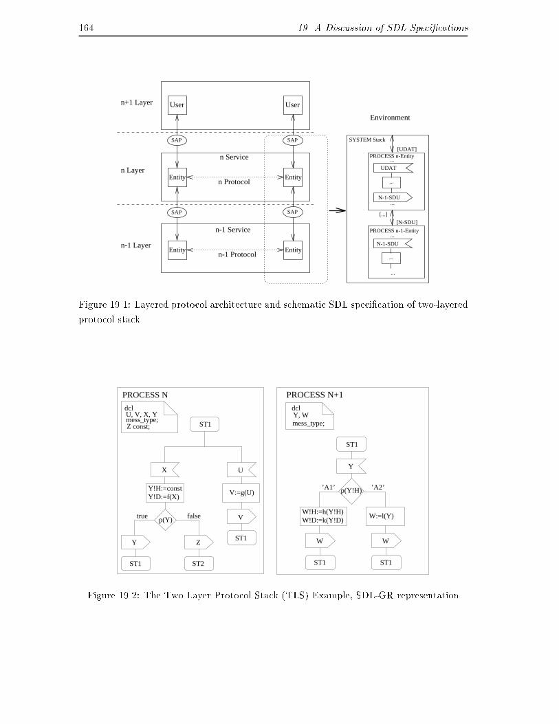
164 19. A Discussion of SDL Speci�cationsn Protocol

EntityEntity

User Usern+1 Layer

n Layer

n-1 Layer

n Service

n-1 Service

SAPSAP

SAP SAP

SYSTEM Stack

[UDAT]

Environment

PROCESS n-Entity...

...

...

...

...

UDAT

...

[...]

[N-SDU]

PROCESS n-1-Entity

N-1-SDU

N-1-SDU

Entity Entityn-1 ProtocolFigure 19.1: Layered protocol architecture and schematic SDL speci�cation of two-layeredprotocol stack.

p(Y)

PROCESS N

dcl

W:=l(Y)

mess_type;

W!D:=k(Y!D)

mess_type;

dcl

ST1ST1

W!H:=h(Y!H)

Y, W

X

Y!H:=constY!D:=f(X)

true false

ZY

ST1 ST2

ST1

U

V:=g(U)

V

ST1

PROCESS N+1

W

U, V, X, Y

Z const;

’A2’

W

p(Y!H)’A1’

Y

ST1

Figure 19.2: The Two Layer Protocol Stack (TLS) Example, SDL-GR representation

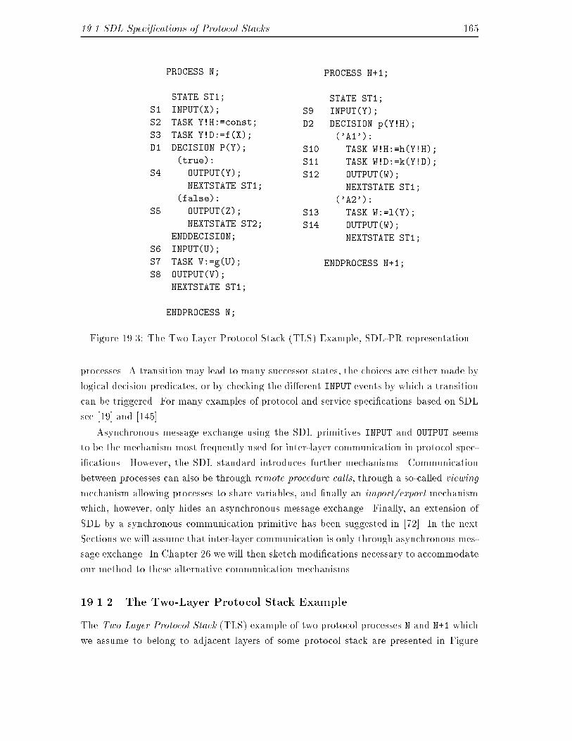
19.1 SDL Speci�cations of Protocol Stacks 165PROCESS N;...STATE ST1;S1 INPUT(X);S2 TASK Y!H:=const;S3 TASK Y!D:=f(X);D1 DECISION P(Y);(true):S4 OUTPUT(Y);NEXTSTATE ST1;(false):S5 OUTPUT(Z);NEXTSTATE ST2;ENDDECISION;S6 INPUT(U);S7 TASK V:=g(U);S8 OUTPUT(V);NEXTSTATE ST1;...ENDPROCESS N;PROCESS N+1;...STATE ST1;S9 INPUT(Y);D2 DECISION p(Y!H);('A1'):S10 TASK W!H:=h(Y!H);S11 TASK W!D:=k(Y!D);S12 OUTPUT(W);NEXTSTATE ST1;('A2'):S13 TASK W:=l(Y);S14 OUTPUT(W);NEXTSTATE ST1;...ENDPROCESS N+1;Figure 19.3: The Two Layer Protocol Stack (TLS) Example, SDL-PR representationprocesses. A transition may lead to many successor states, the choices are either made bylogical decision predicates, or by checking the di�erent INPUT events by which a transitioncan be triggered. For many examples of protocol and service speci�cations based on SDLsee [19] and [145].Asynchronous message exchange using the SDL primitives INPUT and OUTPUT seemsto be the mechanism most frequently used for inter-layer communication in protocol spec-i�cations. However, the SDL standard introduces further mechanisms. Communicationbetween processes can also be through remote procedure calls, through a so-called viewingmechanism allowing processes to share variables, and �nally an import/export mechanismwhich, however, only hides an asynchronous message exchange. Finally, an extension ofSDL by a synchronous communication primitive has been suggested in [72]. In the nextSections we will assume that inter-layer communication is only through asynchronous mes-sage exchange. In Chapter 26 we will then sketch modi�cations necessary to accommodateour method to these alternative communication mechanisms.19.1.2 The Two-Layer Protocol Stack ExampleThe Two Layer Protocol Stack (TLS) example of two protocol processes N and N+1 whichwe assume to belong to adjacent layers of some protocol stack are presented in Figure

166 19. A Discussion of SDL Speci�cations19.21. Both processes are only partially speci�ed:Process N either accepts a message of type X from a non-speci�ed lowerlayer service, which is then processed and sent out as amessage of either type Y or type Z,or it accepts a message of type U which after processing isbeing sent out as a message of type V.Process N+1 accepts a message Y which is processed and sent outas a message W.Hereafter, we shall sometimes abbreviate the terminology by saying a message X insteadof a message of type X. In SDL, the mapping of the output signals of the sending processto the corresponding input signals of the receiving process is done using a relatively com-plicated mapping of signal names to signal routes, where the signal routes carry the senderand receiver identi�cation information. For reasons of conciseness of the presentation wewill use an abstraction of this mechanism and will simply identify sender and receiver ofmessages by the identity of the message type. Thus, in the TLS example the message Ysent out by process N is consumed by process N+1.19.2 Inadequacy of `Faithful' ImplementationsBy the term faithful implementation we refer to an implementation which follows in itsstructure and in the sequence of operations exactly the original SDL speci�cation fromwhich it is derived. This may for example mean (a) that the SDL speci�cation is directlycompiled so that every statement in the SDL speci�cation is mapped to a (sequence of)statement(s) in the implementation, (b) that every SDL process corresponds to a processin the implementation, and (c) that the processes in the implementation communicateusing the SDL asynchronous communication mechanism via in�nite queues. However, aswe argue in the following such a faithful implementation is not e�cient.� No explicit parallelism: Although SDL processes run concurrently the processinginside an SDL process is strictly sequential. This means that the structuring ofthe speci�cation into processes, which in many cases is in uenced by general designdecisions, determines the degree of parallelism of a speci�cation. It also means thatwithout optimizations the sequential processing of operations inside a process maybe ine�cient compared to a parallel execution.1Note that this will be the running example throughout the subsequent development of this part of thethesis.

19.2 Inadequacy of `Faithful' Implementations 167� Structuring of the speci�cation into processes: The structure of the speci�cation oftenmeans that there is one process per protocol layer peer entity of the protocol (see forexample the speci�cations presented in [19] and [145]). The design of communicationprotocols is often governed by the principle that `a good speci�cation is a highlymodular and layered speci�cation'. Though from a structured-design point of view alayered design may be desirable, we stipulate that in order to derive e�cient parallelprotocol implementations such a layered design is obstructive. This is can mainlybe attributed to the fact that the parallel scheduling and combined execution ofoperations belonging to di�erent protocol layers, which can lead to a considerablegain in e�ciency, are inhibited by the layer-wise structuring of the speci�cation.Similar arguments can be found in [46].� Asynchronous inter-layer communication via in�nite queues: An e�cient imple-mentation of a protocol stack for one peer entity will usually be a non-distributedsystem. Apparently it is very ine�cient to implement the exchange of data in anon-distributed system via asynchronous queues. Instead, the protocol data will bestored in a local memory and the communication between the processes will be byshared variables.The objectives of our method are therefore to remove the boundaries between processes, toremove the asynchronous communication between processes, and to analyze dependencesbetween statements so that parallel and combined execution of statements belonging todi�erent processes is enabled.

Chapter 20Dependence Analysis for SDLProcessesIn this Chapter we explain how a data- and control- ow dependence graph can be obtainedby syntactic analysis from an SDL speci�cation. For a de�nition of the mathematicalnotation we use here and in later Chapters see Appendix A. First we will explain howtransitions as basic building blocks of SDL process speci�cations can be formalized andthen how entire protocol stacks can be represented as graphs, built up from the graphsrepresenting single transitions.20.1 Transitions in SDL Speci�cationsSyntactic structure. A transition in an SDL speci�cation is a construct which describesthe transition of an SDL process from one symbolic state into a successor symbolic state.The body of a transition consists of a collection of statements which we group in the set ofstatements S. We only consider a limited subset of SDL-statements, namely INPUT, TASK,DECISION and OUTPUT statements, and we identify one of these four statement types withevery element of S. The statement STATE denotes the current symbolic state and precedesa transition. The statement NEXTSTATE denotes the next symbolic state into which thesystem transits after executing the steps in the transition body. The STATE and NEXTSTATEstatements do not belong to the transition body. We assume that the transition body hasthe following syntactical structure. A transition starts with an INPUT statement. AnINPUT statement may be followed by a TASK, DECISION or OUTPUT statement, or it may bedirectly followed by a NEXTSTATE statement. The TASK statement may be followed by aDECISION, TASK, OUTPUT or NEXTSTATE statement. A DECISION statement may be followedby a TASK, DECISION, OUTPUT or NEXTSTATE statement. An OUTPUT statement is the �nalstatement of a transition and always followed by a NEXTSTATE statement.

170 20. Dependence Analysis for SDL ProcessesJusti�cation. The syntactic subset we have chosen is a reduced subset of the full SDLsyntax. For the sake of conciseness we have limited our considerations to the languagesubset described above but we conjecture that an adequate treatment of other languageconstructs is a straightforward extension. Furthermore, we conjecture that the languagesubset chosen here allows for an analysis of most of the standard protocol speci�cationsas presented in [19].20.2 Control Flow and Data Flow DependencesThe syntactical analysis of the SDL speci�cations that we describe in this Section yieldsa graph structure over the set of statements S of an SDL speci�cation. This so-calleddependence graph identi�es the two types of dependences between members of S, namelycontrol ow and data ow dependences.Dependences. We now describe the di�erent types of dependences between statementsinformally.� Statements, which according to the syntactical and semantical rules of SDL aredirect successors, are part of the control ow dependence relation cfd over the setS. A statement of type DECISION has two or more directly succeeding statements,all pairs of a DECISION statement and it successor statements are part of the cfdrelation. The execution of a statement directly succeeding a DECISION statementdepends on the run-time evaluation of the decision predicate. This is representedby a branching of the cfd graph. We will in later optimization steps, in particularwhen parallelising the dependence graph, have to ensure that statements will onlybe executed when the decision on which they depend has been taken.� A statement usually describes operations on process variables in which these areusually referenced in two di�erent ways.{ We say that a statement Sn uses a variable x i� it references the variablescurrent value without modifying it. Note that in one statement more than onevariable may be used. A typical use of a variable would be to reference its valuein the expression on the right hand side of an assignment statement.{ We say that a statement Sn de�nes a variable x i� it assigns an initial or newvalue to the variable without referencing its previous value. A typical exampleis the de�nition of a variable on the left hand side of an assignment statement.It should be noted that for reasons of simplicity we only allow one variable to bede�ned in one statement, hence all assignment statements are single assignmentstatements.

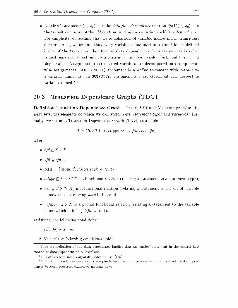
20.3 Transition Dependence Graphs (TDG) 171� A pair of statements (s1; s2) is in the data ow dependence relation dfd if (s1; s2) is inthe transitive closure of the cfd-relation1 and s2 uses a variable which is de�ned in s1.For simplicity we assume that no re-de�nition of variable names inside transitionsoccurs2. Also, we assume that every variable name used in a transition is de�nedinside of the transition, therefore no data dependences from statements in othertransitions exist. Function calls are assumed to have no side-e�ects and to return asingle value. Assignments to structured variables are decomposed into component-wise assignments. An INPUT(X) statement is a de�ne statement with respect toa variable named X , an OUTPUT(Y) statement is a use statement with respect tovariable named Y 3.20.3 Transition Dependence Graphs (TDG)De�nition Transition Dependence Graph. Let S, STT and X denote pairwise dis-joint sets, the elements of which we call statements, statement types and variables. For-mally, we de�ne a Transition Dependence Graph (TDG) as a tupleT = (S; STT; X; sttype; use; de�ne; cfd; dfd)where� cfd � S � S,� dfd � cfd+,� STT = finput; decision; task; outputg,� sttype � S�STT is a functional relation (relating a statement to a statement type),� use � S � P(X) is a functional relation (relating a statement to the set of variablenames which are being used in it), and� de�ne � S �X is a partial functional relation (relating a statement to the variablename which is being de�ned in it),satisfying the following conditions:1. (S; cfd) is a tree.2. 8s 2 S the following conditions hold:1Thus our de�nition of the data dependence implies that an `earlier' statement in the control owcannot be data dependent on a `later' one.2This avoids additional output dependences, see [126].3The data dependences we consider are purely local to the processes, we do not consider data depen-dences between processes caused by message ows.

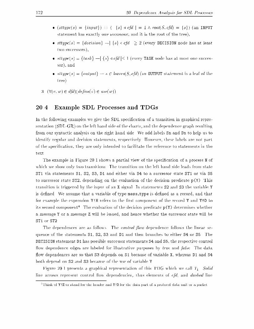
172 20. Dependence Analysis for SDL Processes� (sttype(s) = finputg) $ (j fsg / cfd j = 1 ^ root(S; cfd) = fsg) (an INPUTstatement has exactly one successor, and it is the root of the tree),� sttype(s) = fdecisiong !j fsg / cfd j � 2 (every DECISION node has at leasttwo successors),� sttype(s) = ftaskg !j fsg / cfd j� 1 (every TASK node has at most one succes-sor), and� sttype(s) = foutputg ! s 2 leaves(S; cfd) (an OUTPUT statement is a leaf of thetree).3. (8(v; w) 2 dfd)(de�ne(v) 2 use(w)).20.4 Example SDL Processes and TDGsIn the following examples we give the SDL speci�cation of a transition in graphical repre-sentation (SDL-GR) on the left hand side of the charts, and the dependence graph resultingfrom our syntactic analysis on the right hand side. We add labels Sn and Dn to help us toidentify regular and decision statements, respectively. However, these labels are not partof the speci�cation, they are only intended to facilitate the reference to statements in thetext.The example in Figure 20.1 shows a partial view of the speci�cation of a process N ofwhich we show only two transitions. The transition on the left hand side leads from stateST1 via statements S1, S2, S3, D1 and either via S4 to a successor state ST1 or via S5to successor state ST2, depending on the evaluation of the decision predicate p(Y). Thistransition is triggered by the input of an X signal. In statements S2 and S3 the variable Yis de�ned. We assume that a variable of type mess type is de�ned as a record, and thatfor example the expression Y!H refers to the �rst component of the record Y and Y!D toits second component4. The evaluation of the decision predicate p(Y) determines whethera message Y or a message Z will be issued, and hence whether the successor state will beST1 or ST2.The dependences are as follows. The control ow dependence follows the linear se-quence of the statements S1, S2, S3 and D1 and then branches to either S4 or S5. TheDECISION statement D1 has possible successor statements S4 and S5, the respective control ow dependence edges are labeled for illustrative purposes by true and false. The data ow dependences are so that S3 depends on S1 because of variable X, whereas D1 and S4both depend on S2 and S3 because of the use of variable Y.Figure 20.1 presents a graphical representation of this TDG which we call T1. Solidline arrows represent control ow dependencies, thus elements of cfd, and dashed line4Think of Y!H to stand for the header and Y!D for the data part of a protocol data unit or a packet.

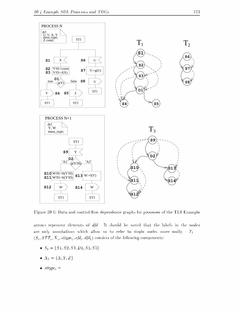
20.4 Example SDL Processes and TDGs 173

W!D:=k(Y!D)

mess_type;Y, Wdcl

ST1

W!H:=h(Y!H)

ST1

PROCESS N+1

WW S14S12

S11

X

Y!H:=constY!D:=f(X)

true false

ZY

ST1 ST2

D1

S2

ST1

U

V:=g(U)

V

ST1

S1

S3

S5

S6

S7

S8p(Y)

S4

PROCESS N

dcl

mess_type;U, V, X, Y

Z const;

W:=l(Y)S10

’A2’

S13

p(Y!H)D2

S9

’A1’

Y

ST1

S7

S6

S3

S5

S1

S2

D1

S4

S8

T1 T2

T3

S9

D2

S10

S11

S13

S14

S12Figure 20.1: Data and control- ow dependence graphs for processes of the TLS Examplearrows represent elements of dfd. It should be noted that the labels in the nodesare only annotations which allow us to refer to single nodes more easily. T1 =(S1; STT1; X1; sttype1; cfd1; dfd1) consists of the following components:� S1 = fS1; S2; S3;D1; S4; S5g� X1 = fX; Y; Zg� sttype1 =

174 20. Dependence Analysis for SDL Processesf(S1; input); (S2; task); (S3; task); (D1; decision); (S4; output); (S5; output)g� use1 = f(S1; ;); (S2; ;); (S3; fXg); (D1; fY g); (S4; fY g); (S5; fZg)g� de�ne1 = f(S1; X); (S2; Y !H); (S3; Y !D)g� cfd1 = f(S1; S2); (S2; S3); (S3;D1); (D1; S4); (D1; S5)g� dfd1 = f(S1; S3); (S2;D1); (S2; S4); (S3;D1); (S3; S4)gWhen in state ST1 process N may execute two di�erent transitions, depending onwhether the signal available at the head of the input queue is of type X or of type U. Abovewe described the transition for the �rst case, for the second case the second transition leadsfrom ST1 via statements S6, S7 and S8 to state ST1. The syntactical analysis as describedabove leads to the transition dependence graph T2 = (S2; STT2; X2; sttype2; cfd2; dfd2)which consists of the following components:� S2 = fS6; S7; S8g� X2 = fU; V g� sttype2 = f(S6; input); (S7; task); (S8; output)g� use2 = f(S6; ;); (S7; fUg); (S8; fV g)g� de�ne2 = f(S6; U); (S7; V )g� cfd2 = f(S6; S7); (S7; S8)g� dfd2 = f(S6; S7); (S7; S8)gFor our later argumentation, which aims at combining multiple processes to one pro-cess, we need a further example SDL process. We will use the process named N+1 �rstpresented in Figure 19.2. The syntactical analysis leads to the transition dependence graphT3 in Figure 20.1. The structure of T3 is quite similar to the structure of T1. It should alsobe noted that the decision D2 does not have a boolean evaluations, instead it evaluatesto strings A1 or A2. Algebraically, T3 = (S3; STT3; X3; sttype3; cfd3; dfd3) consists of thefollowing components:� S3 = fS9; D2; S10; S11; S12; S13; S14g� X3 = fY;Wg� sttype3 = f(S9; input); (D2; decision); (S10; task); (S11; task); (S12; output);(S13; task); (S14; output)g

20.4 Example SDL Processes and TDGs 175� use3 = f(S9; ;); (D2; fY g); (S10; fY g); (S11; fY g); (S12; fWg); (S13; fY g);(S14; fWg)g� de�ne3 = f(S9; Y ); (S10;W ); (S11;W ); (S13;W )g� cfd3 = f(S9; D2); (D2; S10); (S10; S11); (S11; S12); (D2; S13); (S13; S14)g� dfd3 = f(S9; S13); (S9;D2); (S9; S10); (S9; S11); (S13; S14); (S10; S12);(S11; S12)gPreview. The purpose of the transformation of SDL speci�cations into dependencegraphs is to obtain an algebraic representation as input for later optimizations steps (inparticular for the parallelisation). The parallel execution of statements is allowed if theyare neither directly nor indirectly data ow dependent on each other. In TDG T1 in Figure20.1 statement S3 is control ow, but not data dependent on statement S2. This revealsan opportunity for parallelising that we shall exploit later on.

Chapter 21Dependence Graphs for ProtocolStacksAs we saw in Chapter 19 protocol stacks are usually speci�ed by a set of independentconcurrent processes. Each of these processes consists of a number of transitions. InChapter 20 we described how to syntactically analyze each of these processes in order toderive a set of transition dependence graphs for each process. As we argued in Section19.2, it is advantageous to remove the boundaries between layers of SDL processes and toeliminate the inter-layer communication via in�nite queues. In this Chapter we describethe necessary steps to combine the transition dependence graphs of di�erent SDL processesand to remove the communication between them. Technically, we perform this in two steps:� First, we label all TDGs of all processes by so-called input/output labels. Theselabels are the names of the signals exchanged by the INPUT and OUTPUT statementsat the beginning and at the end of each transition.� Second, we combine all TDGs with matching input/output labels, eliminate theOUTPUT(X)/INPUT(X) statement pairs, and perform a cross-layer data dependenceanalysis. We may do this because we assume that every OUTPUT statement can bemapped to a unique INPUT statement of another process. The result is a graph whichwe call Multi-Layer Dependence Graph.21.1 Input/Output labeled Transition Dependence Graphs(IOTDGs)We assume that all transitions we consider for the combination process start with an INPUTstatement accepting a data packet from an adjacent layer process, and end with an OUTPUTstatement which delivers the processed packet to the next adjacent layer process. Hence,

178 21. Dependence Graphs for Protocol Stackswe assume that all the processing for a packet in a layer process is carried out in thecourse of one transition, and that no looping and branching due to JOIN statements insidea transition occurs. Thus, our dependence graphs are always trees. Di�erent transitionsstarting in di�erent states in one process may exist, but they only represent the process tobe in di�erent states (e. g. state waiting and state transmission). Furthermore, we assumethat the packet passing is unidirectional, either from the medium towards the user or viceversa.Formal De�nition of Input/Output labeled TDGs. Based on the above statedassumptions on the structure of the SDL Transitions we formalize the concept of labelingof root and leaf nodes of TDGs by the appropriate signal names as follows. Let T =(S; STT; X; sttype; use; de�ne; cfd; dfd) denote a TDG and let SIG denote a set disjointfrom any other set in sight, the elements of which we call signal names. Furthermore, letinsig � ((S \ root(T )) � SIG) and outsig � ((S \ leaves(T )) � SIG) denote functionalrelations. We de�ne an Input-Output labeled Transition Dependence Graph (IOTDG) asa tuple I = (S; STT; X; SIG; sttype; cfd; dfd; insig; outsig)for which the following conditions hold1:� sttype(root(I)) = input, and� (8x 2 leaves(I))(sttype(x) = output).These two conditions imply that all transitions we consider start with an INPUT statementand end with an OUTPUT statement. In other words, we exclude all those transitions thatdo not end with an OUTPUT statement.Example IOTDG In Figure 21.1 we show the three IOTDGs representing the TDGsfor Example TLS.21.2 Multi-layer Dependence Graph (MLDG)What we have obtained so far is a set T = fT1; : : : ; Tng of IOTDGs. T represents thedependences of all transitions of the speci�cation that we analyze. In this section wedescribe an algorithm that transforms T into a setM of Multi-Layer Dependence Graphs(MLDG). Each MLDG represents the dependences of the processing of one packet orprotocol data unit in adjacent layers of the protocol stack. We are interested in followingthe processing of one packet from the code location where it enters into the protocol stack1We omit the mentioning relations use and de�ne in this and later de�nitions of modi�ed dependencegraphs.

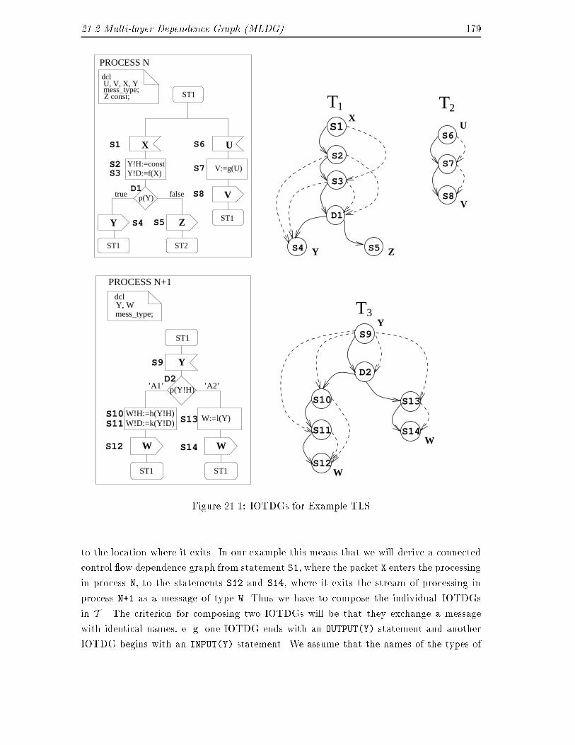
21.2 Multi-layer Dependence Graph (MLDG) 179V

UX

Y

W

W

Y

Z

ZY

UX

V

Y

W W

W:=l(Y)W!D:=k(Y!D)

Y, Wmess_type;

dcl

ST1ST1

W!H:=h(Y!H)

PROCESS N+1

S14S12

S11S10

’A2’

S13

p(Y!H)D2

S9

’A1’

ST1

Z const;

U, V, X, Ymess_type;

dcl

PROCESS N

S4

p(Y) S8

S7

S6

S5

S3

S1

ST1

V:=g(U)

ST1

S2

D1

ST2ST1

falsetrue

Y!D:=f(X)Y!H:=const

3T

2T1T

S12

S14

S13

S11

S10

D2

S9

S5S4

D1

S2

S1

S3

S8

S7

S6

Figure 21.1: IOTDGs for Example TLSto the location where it exits. In our example this means that we will derive a connectedcontrol ow dependence graph from statement S1, where the packet X enters the processingin process N, to the statements S12 and S14, where it exits the stream of processing inprocess N+1 as a message of type W. Thus we have to compose the individual IOTDGsin T . The criterion for composing two IOTDGs will be that they exchange a messagewith identical names, e. g. one IOTDG ends with an OUTPUT(Y) statement and anotherIOTDG begins with an INPUT(Y) statement. We assume that the names of the types of

180 21. Dependence Graphs for Protocol Stacksthe messages exchanged are unique at the interfaces between two processes, and that thedirection of the message ow is uniquely determined by the message type names. Also,we assume that every OUTPUT statement can be mapped to a unique INPUT statement.Note that SDL transitions are deterministic on INPUT signals, i. e. in one state the futurebehavior is uniquely determined by the type of the message that is consumed next.MLDG Construction Algorithm. The functioning of Algorithm 1 is as follows. First,a set T 0 of initial IOTDGs is selected (step I.). This set contains all those IOTDGs thatdo not input a message that is output-ed by another IOTDG. The algorithm then loopsover all these IOTDGs (III.). The set Z (V.) contains all those IOTDGs that can beappended to a leaf node of an IOTDG from T . The next loop (VI.) performs the mergingof two IOTDGs (VII. to XVI.) for all elements of Z . The merging of two IOTDGscomprises the elimination of the two nodes x and root(Z) by which the two graphs aremerged (IX.), this corresponds to the elimination of the OUTPUT/INPUT statements. XIII.describes the construction of the new cfd relation. Every node which depended on root(Z)is made dependent on every node from which x depended. The construction of the newdfd relation (XIV.) is very similar, but we additionally check whether a node on whichx depended de�nes a variable which is used in a node that depended on root(Z). XVII.constructs the result, a set M of MLDGs.

21.2 Multi-layer Dependence Graph (MLDG) 181Algorithm 1I. SELECT T 0 = fT 01; : : : ; T 0mg � T SO THAT(8T 0i)(8Tj)(insig(root(T 0i)) \Sj 6=i outsig(leaves(Tj)) = ;);II. M := ;;III. FOR ALL T 0i 2 T 0IV. M := T 0i ;V. Z := fT 2 T j outsig(leaves(M)) \ (insig(root(T ))) 6= ;g;VI. WHILE Z 6= ;VII. FOR ALL Z 2 ZVIII. SELECT x 2 leaves(M) SO THAT(outsig(x) 2 insig(root(Z)));IX. S0M := SM [ SZ � fxg � root(Z);X. X 0M := XM [XZ ;XII. sttype0M := S0M / (sttypeM [ sttypeZ);XIII. cfd0M := cfdM [ cfdZ � (cfdM . fxg)� (root(Z) / cfdZ)[ fdomain(cfdM . fxg)� range(root(Z) / cfdZ)g;XIV. dfd0M := dfdM [ dfdZ � (dfdM . fxg)� (root(Z) / dfdZ)[f(v; w) 2 fdomain(dfdM .fxg)� range(root(Z)/dfdZ)g j de�ne(v) �use(w)g;XV. M := (S0M ; STTM; X 0M ; sttype0M ; cfd0M ; dfd0M)XVI. Z := fT 2 T j outsig(leaves(M)) \ (insig(root(T ))) 6= ;g;XVII. M :=M[MAs a result we obtain a set of MLDGs M. Each M 2 M is a multi-edged labeled tree(S; STT; X; SIG; sttype; cfd; dfd). Note, however, that not all of the conditions we requiredfor IOTDGs still hold. For example it is not true any more that a node of type input hasno predecessor in the cfd relation.Entry, Exit and Branching Nodes. For a MLDG M we say that a node in root(M)is an entry node, that a node in branchnodes(M) is a branching node, and that a nodein leaves(M) is an exit node. An entry node represents a statement where a message (inmost cases a packet or protocol data unit) is accepted from the environment, and an exitnode refers to a statement in the code where a message is delivered to the environment.Example MLDG Figure 21.2 shows the set M which we obtain by applying our algo-rithm to the IOTDGs of our example TLS. It contains two MLDGs, one with root S1 andone with root S6. Note that the cfd-relation forms the skeleton of the MLDGs. The nodesS4 and S9 have been eliminated, re ecting the elimination of the OUTPUT(Y) / INPUT(Y)statement pair. The additional cfd pair (D1; D2) has been added. Furthermore, data de-

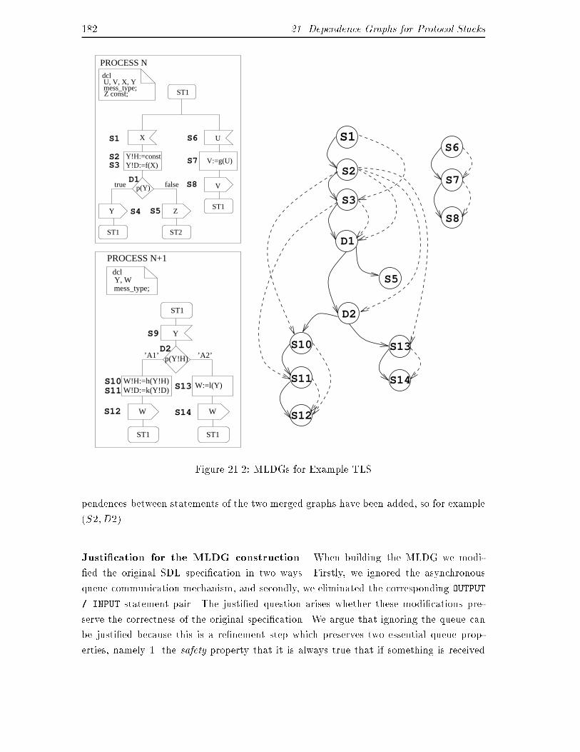
182 21. Dependence Graphs for Protocol StacksST1

S8

S4

PROCESS Ndcl

Z const;

W!D:=k(Y!D)

Y, Wmess_type;

dcl

ST1

X

Y!H:=constY!D:=f(X)

true false

ZY

ST1 ST2

D1

S2

ST1

U

V:=g(U)

V

ST1

S1

S3

S5

S6

S7

p(Y)

mess_type;U, V, X, Y

ST1

W!H:=h(Y!H)

PROCESS N+1

WW S14S12

W:=l(Y)S11

Y

’A1’

S10

’A2’

S13

p(Y!H)D2

S9S10

S11

S13

S14

S12

S3

S1

S2

D1

S5

S6

S7

S8

D2

Figure 21.2: MLDGs for Example TLSpendences between statements of the two merged graphs have been added, so for example(S2; D2).Justi�cation for the MLDG construction. When building the MLDG we modi-�ed the original SDL speci�cation in two ways. Firstly, we ignored the asynchronousqueue communication mechanism, and secondly, we eliminated the corresponding OUTPUT/ INPUT statement pair. The justi�ed question arises whether these modi�cations pre-serve the correctness of the original speci�cation. We argue that ignoring the queue canbe justi�ed because this is a re�nement step which preserves two essential queue prop-erties, namely 1. the safety property that it is always true that if something is received

21.2 Multi-layer Dependence Graph (MLDG) 183it must have been sent before, and 2. the liveness property that it is always true that ifsomething is sent it will eventually be received.The safety property is trivially satis�ed because the order of the OUTPUT(X) andINPUT(X) statements is preserved. The liveness property is satis�ed if we assume ourimplementation to be live, namely that every transition which is continuously enabled willeventually be taken.Furthermore, the elimination of the OUTPUT / INPUT statement pair can be justi�edby the fact that we preserved all control ow and data ow dependences. Thus, the aboveargument concerning the safety properties now holds for all those statements which aredirect predecessors or successors of the OUTPUT / INPUT statements that we eliminated.Another way of looking at it is to consider the traces generated by each of the alter-natives. Let !X stand for an OUTPUT(X) and let ?X stand for an INPUT(X) event and letthe system be in an in�nite loop. Then the language of events that can be observed inthe case of asynchronous queue communication can be described by the !-regular expres-sion (!X+?X+)! whereas our implementation generates the expression (!X?X)!. Hence,the traces generated by our implementation are a subset of the traces allowed by theoriginal SDL speci�cation semantics, and we argue that our implementation is a correctimplementation with respect to a trace inclusion implementation relation.Concluding we can say that out of the many interleavings of events which are possibleaccording to the original speci�cation we only implement one possible representative,namely the interleaving where a packet is accepted at one end of the protocol stack,entirely processed, and �nally handed over at the other end before the next packet isaccepted for processing.As opposed to the ESTELLE related work reported in [71] we do not eliminate theasynchronous queue communication mechanism between adjacent layer processes by re-placing these processes by one product automaton because this would induce an extremeblow-up in the complexity of the implementation.

Chapter 22Determination of the CommonPath GraphThe later steps of our optimization method rely on the assumption that we optimize theprocessing of a packet only for the `common case' (we will come to a clearer understand-ing of this expression in this Chapter). Restricting the optimization to the common casehas the advantage of reducing the complexity of the code that needs to be optimized andtherefore leads to more compact optimized code modules. Furthermore, in Section 23 weintroduce optimization steps that anticipate certain common decision results according toa common case assumption. These optimization steps, which rely on relaxing the depen-dences of statements before and after certain decisions, would be impossible without thecommon case assumption. We consider our common path determination a generalizationof the Common Path optimization as advocated in [35].Protocols usually have the task of hiding imperfect behavior of lower layer servicesfrom upper layer users. This means that a major part of their functionality aims at de-tection and treatment of many kinds of exceptions and errors. Exceptions and errors,however, are usually uncommon, in particular in typical high speed communication envi-ronments. On the other hand, optimizing the common case implies that we need to takecare of uncommon cases using alternate non-optimized error-case implementations. But,as we argued above, because of the low probability of these error handling cases we cantolerate the non-optimized processing of these error cases without risking a considerabledegradation of the performance of the protocol. However, not all branching in the control ow can be classi�ed so that one branch is common and all others are uncommon. It mayas well be the case that more than one alternative is a common choice, namely when thebranching does not aim at handling exception cases.Now, what does the term common case mean technically? We distinguish the decisionedges (outgoing cfd-edges of a node with outdegree > 1) of the cfd relation of an MLDGMdisjointly into those which are taken with a probability above a certain value (the common

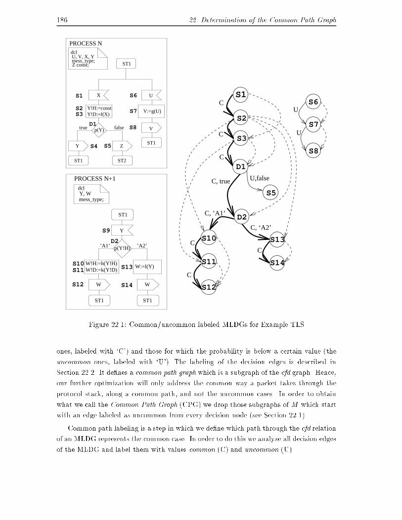
186 22. Determination of the Common Path GraphUX

Y!H:=constY!D:=f(X)

true false

Y

ST1

Y

’A1’

S9

D2p(Y!H)

S13

’A2’

S10S11

S12 S14W W

PROCESS N+1

W!H:=h(Y!H)

ST1 ST1

dcl

mess_type;Y, W

W!D:=k(Y!D)W:=l(Y)

ST1

S6

S7

S8p(Y)

dcl

mess_type;U, V, X, Y

Z const;

ST1

S1

S3

ZS5

ST2

D1

S2

ST1

V:=g(U)

V

PROCESS N

S4

S10

S11

S13

S14

S12

S3

S1

S2

D1

S5

S6

S7

S8

D2

C

C

C

U

C

C

C

C, true U,false

C, ’A1’

C, ‘A2’

U

Figure 22.1: Common/uncommon labeled MLDGs for Example TLSones, labeled with `C') and those for which the probability is below a certain value (theuncommon ones, labeled with `U'). The labeling of the decision edges is described inSection 22.2. It de�nes a common path graph which is a subgraph of the cfd graph. Hence,our further optimization will only address the common way a packet takes through theprotocol stack, along a common path, and not the uncommon cases. In order to obtainwhat we call the Common Path Graph (CPG) we drop those subgraphs of M which startwith an edge labeled as uncommon from every decision node (see Section 22.1).Common path labeling is a step in which we de�ne which path through the cfd relationof an MLDG represents the common case. In order to do this we analyze all decision edgesof the MLDG and label them with values common (C) and uncommon (U).

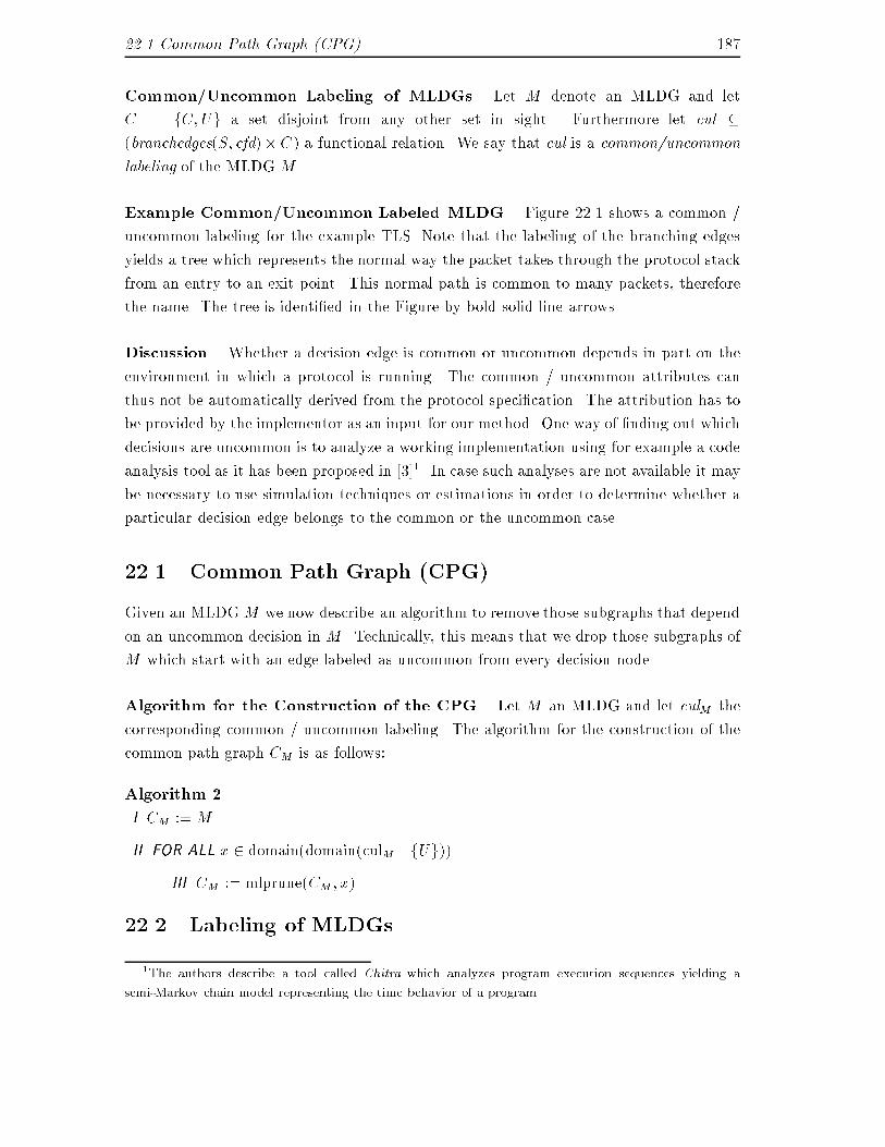
22.1 Common Path Graph (CPG) 187Common/Uncommon Labeling of MLDGs. Let M denote an MLDG and letC = fC;Ug a set disjoint from any other set in sight. Furthermore let cul �(branchedges(S; cfd)� C) a functional relation. We say that cul is a common/uncommonlabeling of the MLDG M .Example Common/Uncommon Labeled MLDG. Figure 22.1 shows a common /uncommon labeling for the example TLS. Note that the labeling of the branching edgesyields a tree which represents the normal way the packet takes through the protocol stackfrom an entry to an exit point. This normal path is common to many packets, thereforethe name. The tree is identi�ed in the Figure by bold solid line arrows.Discussion. Whether a decision edge is common or uncommon depends in part on theenvironment in which a protocol is running. The common / uncommon attributes canthus not be automatically derived from the protocol speci�cation. The attribution has tobe provided by the implementor as an input for our method. One way of �nding out whichdecisions are uncommon is to analyze a working implementation using for example a codeanalysis tool as it has been proposed in [3]1. In case such analyses are not available it maybe necessary to use simulation techniques or estimations in order to determine whether aparticular decision edge belongs to the common or the uncommon case.22.1 Common Path Graph (CPG)Given an MLDGM we now describe an algorithm to remove those subgraphs that dependon an uncommon decision in M . Technically, this means that we drop those subgraphs ofM which start with an edge labeled as uncommon from every decision node.Algorithm for the Construction of the CPG. Let M an MLDG and let culM thecorresponding common / uncommon labeling. The algorithm for the construction of thecommon path graph CM is as follows:Algorithm 2I. CM :=MII. FOR ALL x 2 domain(domain(culM . fUg))III. CM := mlprune(CM ; x)22.2 Labeling of MLDGs1The authors describe a tool called Chitra which analyzes program execution sequences yielding asemi-Markov chain model representing the time behavior of a program.

188 22. Determination of the Common Path GraphS8

S4

PROCESS Ndcl

Z const;

W!D:=k(Y!D)

Y, Wmess_type;

dcl

ST1

X

Y!H:=constY!D:=f(X)

true false

ZY

ST1 ST2

D1

S2

ST1

U

V:=g(U)

V

ST1

S1

S3

S5

S6

S7

p(Y)

mess_type;U, V, X, Y

ST1

W!H:=h(Y!H)

PROCESS N+1

WW S14S12

ST1

S11W:=l(Y)

Y

’A1’

S10

’A2’

S13

p(Y!H)D2

S9

S10

S11

S13

S14

S12

S3

S1

S2

D1

D2

Figure 22.2: CPG for Example TLSExample CPG. In Figure 22.2 we present the CPG derived from the common / un-common labeled MLDG in Figure 22.1. The subgraph starting with the edge (D1; S5) hasbeen removed. The subgraphs starting in node D2 have both been retained as they bothrepresent common branches of a decision. Also, the TDG starting in node S6 has beenremoved as it has no edge belonging to the common path.Preview. In the rest of this document we will focus on the optimization and implemen-tation of the common path of protocols. However, the result of the dependence analysisin Chapter 20 has been a set M of MLDGs, whereas this Chapter only addresses thedetermination of a CPG based on a single MLDG. We expect that the user decides whichelements of M he wishes to be optimized by the later optimization steps, based on asimilar common/uncommon decision as we discussed earlier.

Chapter 23Construction of the RelaxedDependence GraphIn the previous Chapters we have shown how a common path graph (CPG) can be derivedfrom an SDL speci�cation based on a control and data ow dependence analysis. Inthis Chapter we will construct a relaxed dependence graph (RDG) which will be thestarting point for later optimization and implementation steps. The relaxation will bemainly a relaxation of the sequentiality constraints imposed by the sequential control owdependence relations in the CPG. The implementations of the CPG will be, as we argue,correct implementations of the original speci�cation, but they will execute more e�cientlythan `faithful' implementations. The relaxation will consist in the following steps:� Anticipation of the common case: Most nodes in the CPG depend on1 a decisionnode, and normally nodes depending on a decision node can only be executed whenthe last decision node on which they depend has been executed. However, we haveidenti�ed some nodes in the CPG which are of type decision but only have oneoutgoing cfd edge (cf. node D1 in Figure 22.2), so they do not represent a decisionalong the common path. We therefore anticipate the outcome of this decision tobe always the way which we predicted when determining the common path. Wehenceforth treat these decision nodes as nodes representing `normal' statements, andas if no other node depended on their execution. Thereby we reduce the amountof linear sequential execution conditions. We call the resulting graph an anticipatedCPG.� Parallelising: We relax the anticipated CPG such that we �rst strip away the cfdrelation and only retain the dfd relation. However, we need to add some additionaldependences which ensure that a node is never executed before the last decision1For a node x to depend on a node y here means that x is in the transitive closure of the cfd relationrestricted to y on its �rst component.

190 23. Construction of the Relaxed Dependence Graphnode on which it depends in the cfd relation has been executed. The result is aRelaxed Dependence Graph (RDG). In the later implementation two statements canbe executed in parallel i� they do not depend on each other in the RDG.23.1 Anticipation of the Common CaseThe CPG may contain nodes corresponding to decisions with only one outcome belongingto the common path. Decisions enforce an execution order because a node can only beexecuted after all decisions it depends on have been taken. Decisions thus limit potentialparallelism. To enhance potential parallelism we anticipate the outcome of decisions thathave only one outcome in the CPG, which means that we treat such decisions as if theyrepresented nodes of type task instead of nodes of type decision.What does this exactly imply? A successor of an anticipated decision can henceforthbe executed before the outcome of the decision is known. If the outcome corresponds tothe anticipation we have a potential gain in parallelism. However, in the very few caseswhere we process a packet for which our anticipation of the common outcome of a decisionwas wrong, e.g. an erroneous packet has been processed and the error was detected, thenstatements which have already been executed in anticipation of the common outcomeof the decision may need to be undone. In Chapter 25 we discuss the handling of theuncommon case in an implementation and argue that there is always a way to handlethese situations consistently.Anticipation of the common case step is applied to the CPG using Algorithm 3. Givena CPG C, the algorithm selects all decision nodes from the set SC that have only one (I.)and changes the type of these nodes to task (III.).Algorithm 3I. SELECT D = fD1; : : : ; Dmg � SC SO THAT(8Di)((sttype(Di) = decision) ^ (j fDig / cfd j= 1))II. FOR ALL Di 2 D DOIII. sttype(Di) := taskNote that the result of the algorithm is a graph in which all nodes of type decision havemore than one successor in cfd. All decision nodes are thus branching nodes as de�ned in21.1.Example. Anticipating the common case in our example results in changing the state-ment type of D1 from decision to task. When the sequential cfd dependences have beenremoved this will allow us to execute node D1 in Figure 22.2 after node S11.

23.2 Relaxation of Dependences 19123.2 Relaxation of DependencesIn this transformation we remove the cfd dependences from the CPG in order to increasethe potential for parallel execution2. More precisely, we remove all cfd edges, retainthe dfd edges, and add some auxiliary dependences. We obtain a graph, called relaxeddependence graph (RDG), which has the same set of nodes as the anticipated CPG, butonly one dependence relation on its nodes. We call this relation the relaxed dependencerelation (rxd).There are three types of precedence constraints which the relaxed dependence graphhas to enforce:� Data ow dependences: the data ow dependence relation as de�ned by the CPGhas to be respected (a node using a variable may not be executed before a nodewhich de�nes that variable).� Control ow dependences: a node which is (directly or transitively) control owdependent on a decision or root node may not be executed before the decision orroot node has been executed3.� Final execution of exit nodes: Exit nodes must be the last nodes to be executedbecause they are the point where a protocol interacts with its environment andmakes the result of the processing available to the environment. Thus all non-exitnodes must be forced to be executed prior to executing an exit node, and auxiliarydependences need to ensure this.The Algorithm. Starting from an anticipated CPG C we create the RDG and its rxdrelation in three steps. First we include all elements of the original CPG's dfd relation inrxd. This will ensure that data dependences are respected in the RDG. Then we examineeach node of the RDG to see if it already depends (directly or transitively) on its nearestpreceding decision or root node in the original CPG's cfd relation. If not, we add adependence between the examined node and that nearest decision or root node. Thisensures that a node is not executed before the last decision it depends on is executed.Finally, we check whether all exit nodes reachable from a given node in the CPG arealso dependent of that node in the RDG. If this is not the case, then we add relaxeddependences between the given node and the concerned exit nodes. This last step ensuresthat the exit nodes which check whether the anticipations of common outcomes of decisions2By parallel execution of the graph we more precisely mean the parallel execution of the implementationof the statements represented by the nodes of the graph.3Note that some former decision nodes were anticipated in the anticipation step and that these nodeare now considered regular non-decision nodes.

192 23. Construction of the Relaxed Dependence Graphare justi�ed for the respective packet or whether the execution has to be rolled back areactually executed as last steps.Algorithm 4 is the RDG construction algorithm. Starting with an anticipated CPG Cit uses the cfdC and dfdC relations to create the rxd relation over SC � SC of the resultingRDG. The algorithm �rst selects a set D of all decision nodes of the graph plus the root ofthe graph (I.). It includes all elements of dfdC into rxd (II.). Then, for every node x of thegraph, it �nds the nearest node in D from which x is transitively dependent in the cfdCrelation (III.). If in the rxd relation x is not yet transitively dependent of that nearestnode, a new auxiliary dependence is added. Next, all nodes except the exit nodes of thegraph are examined. A dependence is added (V.) between an examined (VI.) node y andeach exit node which is transitively dependent on y in the cfdC relation of the CPG butnot in the rxd relation of the RDG (VII. and VIII.).Algorithm 4I. SELECT D = fD1; : : : ; Dmg � SC SO THAT(8Di)(sttype(Di) = decision _Di = root(C))II. rxd := dfdCIII. FOR ALL n 2 SC � root(C)IV. SELECT Dn SO THATfs 2 D j (s; n) 2 cfd+C ^ (Dn; s) 2 cfd+Cg = ;V. IF (Dn; n) =2 rxd+ THEN rxd := rxd [ f(Dn; n)gVI. FOR ALL m 2 S � leaves(C)VII. FOR ALL x 2 leaves(C)VIII. IF (m; x) 2 cfd+C ^ (m; x) =2 rxd+ THENrxd := rxd [ f(m; x)gWe call the resulting directed graph R = (SC; rxd) the relaxed dependence graph forCPG C. It should be noted that R is not a tree any more.Example. Figure 23.1 shows the RDG for the anticipated CPG in Figure 22.2. Thedependence graph in the middle is the one obtained after executing step II of the algorithmwhen only the dfd relation of the original graph is retained. The complete RDG is shownon the right hand side of the Figure. It is obtained by adding auxiliary dependences. Inorder to ensure the dependence of nodes from their closest decision or root node the edges(S1; S2); (D2; S10); (D2; S11) and (D2; S13) have been added. In order to ensure that theexit nodes S12 and S14 are actually executed last, and to avoid the anticipated decisionnode D1 to be executed last, the dependences (D1; S12) and (D1; S14) were added. Wesee that S2 and S3 depend both on S1, but they do not depend on each other. This meansthat once S1 has been executed S2 and S3 can be executed in parallel.

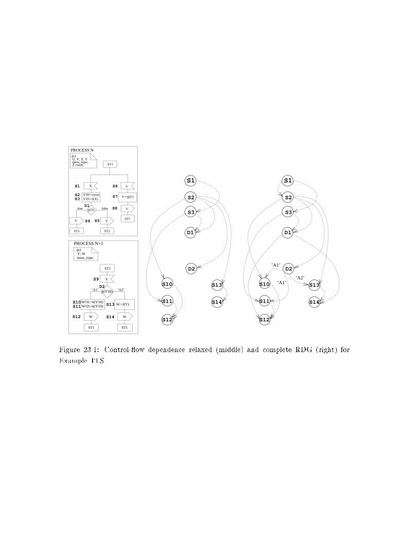
S10

S8

S4

PROCESS Ndcl

Z const;

W!D:=k(Y!D)

Y, Wmess_type;

dcl

ST1

X

Y!H:=constY!D:=f(X)

true false

ZY

ST1 ST2

D1

S2

ST1

U

V:=g(U)

V

ST1

S1

S3

S5

S6

S7

p(Y)

mess_type;U, V, X, Y

ST1

W!H:=h(Y!H)

PROCESS N+1

WW S14S12

ST1

S11

Y

’A1’

W:=l(Y)

’A2’

S13

p(Y!H)D2

S9S10

S11

S13

S14

S12

S3

S1

S2

D1

D2

’A1’

’A1’

’A2’S10

S11

S13

S14

S12

S3

S1

S2

D1

D2Figure 23.1: Control- ow dependence relaxed (middle) and complete RDG (right) forExample TLS

194 23. Construction of the Relaxed Dependence Graph

Chapter 24Optimizations based on the RDGThe RDG will be the basis for an implementation of the common path portion of theprotocol stack. The run-time or compile-time scheduling of the operations in the RDG ona given hardware architecture is an important task of an implementation. When schedulingthe operations, the scheduler may take advantage of the relaxation of dependences in theRDG. In particular, relative to other operations the execution of an operation may bescheduled in an order di�erent from the order prescribed in the original sequential SDLspeci�cation. Therefore, the scheduler may schedule the processing of certain operationswhenever it seems optimal, for example when the required resources and data are available.This also ensures that the inherent potential for parallelism in the RDG can be exploited.A further gain in e�ciency can be achieved by combining the execution of so-called DataManipulation Operations (DMOs), which also depends on some freedom in the ordering ofoperations. In the next Section we will discuss how this concept can be interpreted basedon an RDG.24.1 Grouping of Data Manipulation Operations.We call data manipulation operations (DMOs) operations that manipulate entire dataparts of protocol data units. Examples are checksum calculation and encryption of data.Combining two such operations into one that does two manipulations at the same timesaves an extra storing and fetching of all the data and therefore executes much faster thanthe non-combined execution of both operations. This has already been demonstrated in[35]. It is also central to the work reported in [36] and [2]. Particularly, it has been shownin [123] that in presence of decisions along the path of execution of a packet in the protocolstack it is advantageous to wait with the execution of DMOs until all decisions have beentaken. At that point the set of DMOs to be executed is known and the DMOs can becombined. The technique of deferment of the execution of operations is referred to as lazymessages in the literature.

196 24. Optimizations based on the RDGIn this section we present an algorithm which manipulates the RDG such that thescheduler is enabled to schedule the execution of DMOs in a combined fashion. Thealgorithm is a generalization of the `lazy messages' technique. The grouping of DMOsmeans that we tightly couple the processing of operations which in the RDG are notdependent, so that their joint processing requires less execution time. In order to enablejoint scheduling of operations the RDG has to be modi�ed. It has to be taken intoaccount that when grouping the execution of two DMOs so that one operation dependson a decision higher up in the RDG than the other operation, the higher operation mustbe executed along every possible path through the RDG. It is thus necessary to distributeDMOs over the RDG.Example. Let us assume that the operations S3 (TASK Y!D:=f(X)) and S11 (TASKW!D:=k(Y!D)) in the TLS example (see Figure 23.1) are DMOs. In a real-world exampleS3 might be a translation routine translating every byte of the message X and assigningit to the data part of message Y, whereas S11 might be another such operation on thesame data resulting in the data part of message W. The identi�cation of DMOs as such isa manual task here, however, it is certainly possible to partly automate the detection ofDMOs in the SDL speci�cation.We include all identi�ed DMOs in an RDG in a set called DMO, hence in this exampleDMO = fS3; S11g. However, in order to allow two DMOs to be combined the followingcondition needs to be satis�ed. It is necessary to require that there may not exist a nodewhich is rxd dependent on one DMO, so that the second DMO is rxd dependent on thisnode. Such a node would clearly have to be executed after the �rst DMO but beforethe second, thus defeating the combined execution of the DMOs. For two DMOs to beexecuted at the same time, all decisions on which their execution depends must have beentaken before the combined execution can be permitted. In our TLS example, even if S3does not depend on D2 we would nevertheless have to execute S3 after D2 because onlythen we know if S11 will need to be executed at all. To make sure that S3 is executedafter D2 we modify the RDG so that S3 depends directly on D2 rather than on S1, thenode it is originally depending on in the RDG.We have, however, to take into account that S3 will have to be executed independentlyof what the evaluation of the decision node D2 is. Thus we need to \distribute" S3 overall possible evaluations of D2, or, more precisely, over all subgraphs with root note D2.Distributing a DMO over the possible evaluations of a decision predicate means that wemake one copy of the node representing the DMO for each possible outcome of the decision.In our example there will be two copies, one corresponding to the 'A1' evaluation of D2(we'll call this new node S301), and one to corresponding to the 'A2' evaluation (S302). IfD2 evaluates to 'A2' we can execute a combined DMO S302/S11. If D2 evaluates to 'A1',then we execute S301 alone.

24.2 An Algorithm for Grouping of DMOs 19724.2 An Algorithm for Grouping of DMOsWe propose a recursive algorithm that starts at the root of a given RDG (see Algorithm5). The algorithm is �rst applied to the root node of a RDG C, and then recursively tothe whole rest of the graph. The algorithm also takes as input the cfd relation of the CPGfrom which the RDG C was originally derived. This will help in determining from whichclosest decision or root node a node is cfd dependent. Let B be the name of the node thealgorithm is currently applied to. The algorithm distributes the DMOs that depend onB over each decision depending on B (we refer to any one of these as B0) if and only ifother DMOs exist which can only be executed after B0. The algorithm is then recursivelyapplied to all decisions B0 which depend on B.Starting from a node B, the algorithm functions as follows. For each DMO D whichdepends on B (I.) a second DMO D2 depending on another decision node is searchedin the subset of nodes that may be executed1 if D is executed (II.). If such a DMOexists, the decision node B0 depending on B and leading to D2 is found (III.). Then Dis removed from the graph (IV.-VI.) and several copies of D, called D0i, are created, onefor each possible evaluation of B0 (VII.-X.). Dependences are added from D0i to all exitnodes which can be reached from B0 with the corresponding evaluation of the predicate(XI.). Once all DMOs depending on B have been treated, the algorithm is applied toall decision nodes depending on B (XII. and XIII.). The algorithm stops when B has no1In the algorithm this subset is found using the transitive closure of the cfd relation of the originalCPG.

198 24. Optimizations based on the RDGmore successors which are decision nodes.Algorithm 5RecursiveCombine(B)I. FOR ALL fD 2 DMO j (B;D) 2 rxdgII. IF 9D2 2 DMO j (D;D2) 2 cfd+ ANDfs 2 SC j (D; s) 2 rxd+ ^ (s;D2) 2 rxd+g = ;III. B0 = s 2 branchnodes(C) j (B; s) 2 rxd ^ (s;D2) 2 rxd+IV. SC := SC � fDgV. DMO := DMO � fDgVI. rxd := rxd � fD / rxd [ rxd . DgVII. FOR ALL Ni 2 B0 / cfdVIII. SC := SC [ fD0igIX. DMO := DMO [ fD0igX. rxd := rxd [ (B0; D0i)XI. rxd := rxd [ f(D0i; x); x 2 leaves(C) j (Ni; x) 2 cfd+gXII. FOR all nodes newB 2 B / rxd and sttype(newB) = decisionXIII. call RecursiveCombine(newB)The algorithm creates groups of DMOs that are selected by the same evaluation ofa decision. Such groups of DMOs can be combined to one complex DMO which canbe implemented in a much more e�cient way. The actual rewriting of the DMOs intoone complex DMO is done during implementation. One method for doing this has beensuggested in [2].Example. An application of the algorithm to our example is exempli�ed in Figure 24.1.We de�ned two nodes, namely S3 and S11, to be DMOs. S3 is replicated for eachevaluation of D2, yielding S301 and S302. If D2 evaluates to 'A1' then a combined DMOS301=S11 can be executed. If D2 evaluates to 'A2', then S302 is executed alone. In the�nal implementation the schedule of the operations has to be such that depending on theevaluation of the decision predicate D2 either S301 or S302 is executed before D1, but notboth.

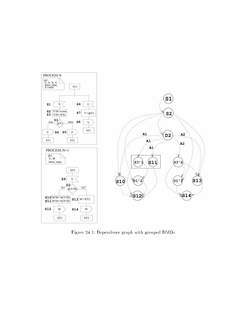
S8p(Y)

S4

PROCESS Ndcl

Z const;

W!D:=k(Y!D)

Y, Wmess_type;

dcl

ST1

X

Y!H:=constY!D:=f(X)

true false

ZY

ST1 ST2

D1

S2

ST1

U

V:=g(U)

V

ST1

S1

S3

S5

S6

S7

ST1

W!H:=h(Y!H)

mess_type;U, V, X, Y

WW S14S12

S11

PROCESS N+1

W:=l(Y)

ST1

Y

’A1’

S10

’A2’

S13

p(Y!H)D2

S9

S12

S10

S11

S14

S1

S2

D2

S13

S3’1 S3’2

D1’2 D1’1

A1

A1 A2

A2A1

Figure 24.1: Dependence graph with grouped DMOs

200 24. Optimizations based on the RDG

Chapter 25Implementing the OptimizedGraphIn the previous chapters we have shown how a multi-layer dependence graph (MLDG) canbe derived from an SDL speci�cation, how a common path graph (CPG) can be extractedfrom the MLDG, and how this CPG can be transformed into a relaxed dependence graph(RDG). This chapter addresses �nal aspects of the method, namely the implementationof the considered protocol stack based on the derived RDG.Implementing the RDG means that we map the statements corresponding to each nodeto a set of software- or hardware instructions. When performing this mapping we have toconsider the following three aspects:� First, we have to respect the ordering constraints on the operations as speci�ed bythe rxd relation of the RDG.� Second, assuming the availability of parallel processing resources, the operationshave to be scheduled on the hardware resources according to the ordering constraints,the qualitative resource requirements, and the expected time consumption of everyoperation on particular hardware components.� Finally, we have to take care of the fact that the RDG only describes the commoncase of packet processing, i. e. we need to provide for an alternate processing whena packet belongs to an uncommon case. This includes assuring that the system is ina consistent state after a packet has been detected not to comply with the commoncase.

202 25. Implementing the Optimized Graph25.1 Preserving Ordering ConstraintsThe RDG imposes a set of ordering constraints on the operations to be executed. Ingeneral, this is a partial order. If we look back at the RDG in Figure 23.1 it is easy tosee that for the subset fD2; S10; S11g of operations the following partial order, expressedinformally in terms of a process algebra like behavior expression, is (D2; (S10 || S11)).Any interleaving trace derived from this expression is the trace of a valid implementation,e. g. the traces (D2; S10; S11) and (D2; S11; S10). However, for the exact derivation of anoptimal implementation these possible interleavings do not provide su�cient information,in particular for the following two reasons.� The operations may be executed in a machine environment with limited parallel pro-cessing resources, so the theoretical maximal possible degree of parallelism may notalways be attainable. Also, the processing resources may not be homogeneous andcertain operations may have particular requirements of the particular characteristicsof the resources on which they are to be executed.� Furthermore, operations are not atomic, as the interleaving model suggests, but theyhave a duration. This also means that they may be executed partly simultaneously,and one operation may be executed simultaneously with a sequence of di�erent otheroperations. All relations that are valid for two or more convex intervals are possiblefor the operations in the RDG. However, for two operations A and B where Bdepends on A we require that A has to be �nished before B starts.25.2 SchedulingConcludingly, the RDG de�nes ordering constraints on the operations that need to beexecuted in an implementation. However, in order to come to an implementation thetarget hardware architecture also has to be taken into account. Assuming that the im-plementation is supposed to run on a parallel hardware architecture this leads to theproblem of deriving an optimal schedule. The schedule does not only re ect the order ofthe execution of operations, but also answers questions about how long an operation willoccupy a certain hardware component. Last, because we cannot assume that all parallelcomponents of the hardware have equal qualitative characteristics, the schedule will alsohave to respect qualitative constraints, like which operation has to be executed on whichhardware component.

25.3 Ensuring Consistency - Treatment of Uncommon Cases 20325.3 Ensuring Consistency - Treatment of UncommonCasesThe RDG we derived from the initial speci�cation is based on the so-called common caseassumption. This means that we assume that the packets processed inside the RDG allcomply with the assumptions made to determine the common path through the protocolstack, e.g. that they are error-free, that they do not require exception handling etc. As aconsequence we anticipated the results of some of the decisions along the common path.This means that we presumed a certain evaluation of some of the decisions and removeddependences of statements depending on these presumed decisions. In other words, someoperations have been decoupled from the decision predicates by which they were `guarded'in the original speci�cation. This may lead to inconsistent sequences of operation. Forexample, a division by zero may be executed concurrently with the test for non-zeronessof the respective operand if we assumed that non-zeroness is the common case. In theoriginal speci�cation of our example TLS (see Figure 20.1) the execution of D2 (throughS4) depends on the evaluation of decision D1 to true. However, in the RDG in Figure 23.1S4 does not depend on the evaluation of D1. This implies that D2 may even be executedbefore D1 is evaluated. A possible inconsistency can only be detected when the processingof a packet reaches an exit node.Apparently, consistency ensuring mechanisms have to be applied. This leads to thefollowing three requirements.� First, as we argued before we need to have a faithful and complete backup imple-mentation of the whole protocol stack available. The backup implementation coversall decisions, exception handling mechanisms etc. as foreseen in the original spec-i�cation. It takes over control when the optimized implementation detects that apacket violates the common case assumption, namely if a test does not evaluate tothe value which was anticipated during the common path determination.� Second, because we saw that operations may be executed prior to the evaluation ofa decision predicate by which they were originally guarded, all operations must berobust. This means that no matter when an operation is executed it is ensured thatthe system will not enter a failure state.� Third, when the processing control is handed over to the classical implementation,the state of the system when the packet has entered the protocol stack through anentry node has to be reestablished. To ensure that this initial state can always bereestablished we suggest using the following mechanism.{ We distinguish operations in reversible and irreversible operations. We claimthat most operations are irreversible, in particular operations reading data or

204 25. Implementing the Optimized Graphcopying data from one storage location into a register, modifying the data, andwriting it to a second storage location. Operations of this sort are reversible(because the unmodi�ed data is still available in the old location), and theycan easily be undone when control needs to be transferred to the backup im-plementation.{ All those operations which are irreversible, and we claim that that is only aminor part of all operations, need to be secured by a checkpointing mecha-nism. This means that the data which is a�ected by these operations will becheckpointed before the respective operation is executed. If not all decisionsare evaluated in the way it was anticipated, i. e. the packet is not processedaccording to the common case, the checkpoint information can be used to undoall irreversible operations.Discussion. It arises the justi�ed question how advantageous our optimization is in lightof these time consuming consistency ensuring mechanisms. We claim that the resetting tothe initial state only occurs very infrequently, namely when an uncommon case has beenreached. This holds in particular in high speed communication protocols where error ratesare low, and ow control mechanisms are very often omitted. Also, we think that onlyvery few operations in high speed protocols are reversible and require a checkpointing forthe state of the protocol stack. However, when uncommon cases occur more and moreoften it is clear that there will be a break-even point between the e�ciency gain due to theparallel and resequenced operation, and the resource consumption for consistency ensuringmechanisms.25.4 Case Study: an IP/TCP/FTP Protocol StackIn [107] we presented the application of an earlier version of our method to the SDLspeci�cation of an IP/TCP/FTP protocol stack. The SDL speci�cation on which we basedthis example was developed in the context of our work. We �rst mapped operations orsequences of operations in the protocol stack to statements in the SDL speci�cation. (Thegranularity of the resulting set of operations in the SDL speci�cation greatly in uencesthe complexity of the dependence graphs). We identi�ed 21 statements (operations anddecisions) in the speci�cation. Some of the operations were procedure calls which hidmore complex operations. We determined a common path, constructed a dependencegraph, and determined a relaxed dependence graph.Based on the relaxed dependence graph we combined two DMOs, namely the TCPchecksum calculation, and the translation from internal into external ASCII representationinside the FTP layer. We scheduled the operations on a hardware architecture withlimited parallelism which consisted of independent medium and host interface components,

25.4 Case Study: an IP/TCP/FTP Protocol Stack 205two FIFO queues feeding the interfaces, a special purpose Data Manipulation Unit, ageneral purpose microprocessor, and a random access memory unit. We assigned resourceconsumptions and qualitative resource constraints to each of the operations, and appliedan enumerative scheduling algorithm to this problem.In the optimal schedule the both DMOs were executed jointly, and in parallel withother operations (both DMOs were scheduled to be executed on the data manipulationunit, whereas the other operations were executed in parallel on the microprocessor). Theoptimal schedule would have been executed within 413 process cycle time units, whereasthe strictly sequential execution of the packet processing along the common path in a`faithful' fashion according to the SDL speci�cation would have taken 1036 processorcycle time units.

Chapter 26Alternative SDL CommunicationMechanismsWe assumed that the inter-layer communication mechanism in the SDL protocol stackspeci�cation relies on the asynchronous exchange of messages by means of INPUT andOUTPUT statements. For all we know, this is the common way to specify data exchange atlayer interfaces in SDL speci�cations, c.f. the many examples in [19] and [145]. However,SDL o�ers alternative inter-process communication mechanisms. We do not know whetherthese are used anywhere for specifying inter-layer communications, and we do not neces-sarily recommend using them for this purpose, however we feel that a short discussionof how our dependence analysis method extends to these communication mechanisms isnecessary.We shall discuss the following alternative communication mechanisms in the followingSections: [72] suggests extending SDL by a synchronous communication primitive. TheSDL-92 standard [32] introduces a synchronous communication mechanism by means of aremote procedure call (rpc) mechanism (c.f. [53]). Furthermore, there are two mechanismswhich rely on so-called shared values, namely the viewing mechanism and the export andimport of variable values.26.1 Synchronous Communication Primitive[72] suggests extending SDL by a multi-way synchronization primitive calledSYNCHRONIZATION. It refers to a signal type, and all processes having this signal typein their input alphabet (or, more precisely, having this signal type in their incoming signallist) will have to synchronize in order to jointly execute the synchronization statement.Note that this is only a proposed extension and not included in the current SDL standard.Let us restrict the multiway synchronization to the two process case and let us assumethat a process A wishes to synchronize with process B by sending a signal of type X.

208 26. Alternative SDL Communication MechanismsLet us furthermore assume that X has one parameter, and that upon synchronization Awants to assign the value of the parameter to a variable u, whereas B wants to �ll theparameter position with the value of its variable v. Finally, let both A and B have signalname X on their incoming signal list. Then, A would contain a SYNCHRONIZATION X(?u)and B would contain a SYNCHRONIZATION X(!v) statement. Both statements will only beexecuted in the course of one atomic action if in one global system state both processes areprepared to execute the synchronization. Note that like the synchronous communicationmechanism we de�ned in Section 7.9 for MFGs and MSCs the synchronization here isdirected, representing a direction of data ow.In the context of the dependence analysis for inter-layer communications in the protocolstack the SYNCHRONIZATION X(?u) is a de�ne statement with respect to variable u. TheSYNCHRONIZATION X(!v) statement is a use statement with respect to variable v. Notethat one SYNCHRONIZATION statement may contain data ows in di�erent directions.26.2 Remote Procedure CallsSynchronous communication has been introduced into the SDL-92 standard by means ofa remote procedure call (rpc) mechanism. Procedures can return values, and if they arelabeled exported, then they can be declared as imported by another process. This otherprocess may call such a remote procedure and receive the return value of the procedure.The calling process will be blocked until the remote procedure terminates.As mentioned above we currently do not know of any example of the use of remoteprocedure calls for inter-layer communication, but in principle the rpcs could be used forthis purpose in the following way. Assume that a process A wishes to receive a value fromprocess B, and that process B has this value stored in a variable U. Furthermore, assumethat B contains the declaration of a remote procedure P which does nothing else thantaking the global variable U, assigning it to a reserved name called result (i.e. result :=U), and then terminates1. The value in result will be the value returned to the callingprocess. Now, to achieve synchronization, process B has to be in a state in which it canexecute P (for details concerning when this is the case see [53]), and process A has to callP by executing a V := call P statement. A will be blocked until the value of P has beenreturned and assigned to V. According to [53] the noti�cation of a call to the procedure Pas well as the noti�cation that P has been executed and the return of the result value isimplemented as an implicit asynchronous signal exchange. Hence, the rpc mechanism ismerely an implicit protocol enforcing process synchronization, based on the standard SDLasynchronous signal exchange mechanism.1Note that remote procedures are local scope units, but variables of the global scope are accessible andmodifyable.

26.3 Shared Values 209From the point of view of the data ow dependence analysis the above scenario wouldneed to be treated in the following way. Inside process A the V := call P statement isa de�ne with respect to the variable V. However, to determine the dependences relatingto the procedure call requires some more apparatus, and for an exact de�nition of thedependence analysis we refer the reader to [56]. Informally, the V := call P statementis of course also an indirect use statement with respect to the variable U of process P.26.3 Shared ValuesViewing Mechanism. The viewing mechanism allows to access variables de�ned inother processes within the same block. A process A making a variable X available to an-other process would declare this variable as revealed: dcl revealed X ...;. The processB would access the value of X by a view statement: view (process A X);. Apparently,the assignment of a value to X in process A would mean a de�ne of the variable. In processB, the access of the variable X of process A would mean a de�ne of the variable A insidethe scope of process B. According to [145] the usage of the viewing mechanism is not rec-ommended and is only included in the SDL language for backwards compatibility reasonswith older versions. Also, it should be noticed that the viewing mechanism provides forno synchronization between the processes, i.e. the process B in the above example will notknow when the value of variable X has been updated. To make this communication mecha-nism useful in the context of inter-layer communication would require the implementationof additional synchronization mechanisms.Import and Export. A process A may export a variable X, which has been declaredexported, by executing the statement export(X). A process B may import the variable byuse of an import statement, for example in the course of the following assignment: taskY:= import(X, A). It should be noted that according to [19, 145] the export/importmechanism is implemented as an asynchronous signal exchange like for OUTPUT and INPUTstatements. Hence, the import/export mechanism is not a true shared memorymechanism.The treatment with respect to the data ow analysis is hence similar to the treatment ofOUTPUT and INPUT statements. The export(X) statement is a use of variable X, whiletask Y:= import(X, A) is both a de�ne of X in the process scope of B and a use of A, aswell as of course a de�ne with respect to Y.

Chapter 27ConclusionsIn this Part of the thesis we presented formalizations and algorithms for the derivation ofoptimized protocol implementations from SDL speci�cations. We started with a syntac-tical dependence analysis for SDL processes. We then showed how multiple dependencegraphs can be combined to multi-layer dependence graphs. Next we determined the com-mon path graph, a subgraph of a multi-layer dependence graph which represents thecommon case of processing of a packet in the protocol stack. This graph was the ba-sis for an optimization by anticipating the evaluation of some decision statements in theCPG, and then by relaxing the dependences. This essentially meant to omit control owdependences and to only consider data ow dependences and dependences that expressthe dependence of a statement from the evaluation of a decision predicate. We called theresult a relaxed dependence graph. When scheduling the operations on a given hardwarearchitecture the scheduler may take advantage of the relaxation of dependences in theRDG in particular by scheduling certain operations at a di�erent point of time comparedto the sequential execution in the SDL speci�cation. In particular we showed how theoptimization concepts of lazy messages and grouping of Data Manipulation Operationscan be interpreted based on the Relaxed Dependence Graph.In general, implementing the RDG means that we map the statements correspondingto each node to a set of software instructions or hardware modules. When performingthis mapping we have to consider three aspects. First, we have to preserve the orderingconstraints imposed by the RDG. Second, assuming the availability of parallel processingresources the operations have to be scheduled according to the ordering constraints, theresource requirements and the expected time consumption of every operation. Finally wehave to take care of the fact that our RDG only addresses the common case, i. e. we needto solve the problem of the alternate processing when a packet belongs to the uncommoncase. A preliminary description of these implementation aspects is given in [107] (see alsoChapter 25).

212 27. Conclusions

Part VConclusion

Chapter 28Concluding RemarksWe arrived at the point where it is time to recapitulate the chief technical arguments madeso far, and to point at directions for future research.28.1 RecapitulationWe have been addressing two major problems arising from the use of formal methods inthe telecommunications systems engineering process.Speci�cation and SemanticsFirst, we were concerned with formal semantics for speci�cation methods in telecommu-nications systems engineering.Semantics for Message Flow Graphs and Message Sequence Charts. We werelooking in particular at a speci�cation formalism called Message Sequence Chart, whichis a specialization of the Message Flow Graph concept. We noticed their occurrences indi�erent domains of software engineering, namely in telecommunications engineering butalso in the analysis of concurrent code and in object models, and we argued for a need tode�ne a formal semantics for these charts.Our requirements were that the semantics are in�nite traces of interleaved communi-cation events, and that these traces have to be representable by a �nite state automatonbecause MFG and MSC speci�cations represent inherently �nite-state systems. We fur-thermore required that the semantics handles both asynchronous and synchronous commu-nications, even in the same chart. We brie y described the requirements on the GEODEtoolset and observed that it shares the �nite-state assumption with our semantics.The basic model we chose as representation for the sets of traces speci�ed by an MFGwas the B�uchi automaton, however we noticed that liveness properties are underspeci-�ed in MFG speci�cations, and that these need to be added to MFG speci�cations in

216 28. Concluding Remarksorder to determine the end-state selection criteria for the B�uchi automaton. We noticedthat temporal logic can be a more exible tool for the speci�cation of liveness propertiescompared to the de�nition of end-state sets for the B�uchi automaton, and we showedhow to interpret the global state transition graphs resulting from our interpretation of anMFG speci�cation as models of propositional linear time temporal logic. Furthermore, weproved that MFG speci�cation are expressibly equivalent to B�uchi automata.We located problems and ambiguities in some of the concepts underlying MFG spec-i�cations. First, we showed that the unimpeded use of conditions in MFG speci�cationsleads to non-local choice conditions. The resolution of these hinges on the availability ofhidden devices capable of remembering potentially unbounded execution histories, whichcontradicts our �nite-stateness requirement. Furthermore, we proved that crossing mes-sage arrowsmay entail hidden and non-explicit assumptions on the environment behaviour,in our view an undesirable feature.We also investigated the ITU-T standards document Z.120 for MSCs and its AppendixB which standardizes a Process Algebra Based semantics, and we related our approachto both documents. We discussed problems in the relation of the textual and the graph-ical representation of MSCs as described in Z.120. This entailed as we showed that thesemantics in Annex B of Z.120, which relies on the textual representation of MSCs, isnot based on a well-de�ned language. Furthermore, we criticised that from a pragmaticviewpoint the process algebra based semantics of Z.120 Annex B is the less useful one,because it avails itself to state based veri�cation methods only indirectly by means of afurther translation step.Quality of Service Speci�cation. We noted that hard real-time constraints are animportant class of requirements in telecommunications systems engineering, and that thesemantics of the speci�cation language SDL is inexpressive with respect to hard real-time constraints. This is mainly due to the timer mechanism relying on asynchronousmessage exchange. We put forward the idea to use real-time extended temporal logics asa complement to SDL speci�cations in order to express hard real-time constraints.This entailed the de�nition of a common model theoretic foundation for SDL andlinear time temporal logic. In the course of doing so we exempli�ed how SDL can beinterpreted in terms of logic, and we clari�ed the relation of symbolic states and systemstates in SDL speci�cations. By usage of complementary Metric Temporal Logic (MTL)formulas in combination with SDL speci�cations we showed how to specify a number ofreal-time related Quality of Service constraints for SDL speci�cations. The previouslyde�ned state-transition based semantics for MFGs allowed us to use MTL speci�cationsalso in combination with MFGs and MSCs.

28.2 Directions for Future Research 217ImplementationNext we considered a method for the derivation of optimized, parallel implementationsfrom SDL speci�cations of protocol stacks. We argued that the e�ciency of the protocolprocessing is crucial because communication bandwidths have increased signi�cantly inrecent years and turned the protocol processing machines into a performance bottleneck.First, we noted that it is ine�cient to implement SDL speci�cations of protocol stacks`faithfully'. We noted that in particular sequential control ow dependences as well as thebu�ered inter process communication mechanism and the distribution of protocol functionsof di�erent processes obstruct an e�cient implementation.To overcome this de�ciency we suggested a data- and control ow analysis of thetransitions in SDL processes. Then we assumed that packets are processed in a sequenceof steps on their way through the protocol stack and we removed the boundaries betweendi�erent protocol layers. Next we determined a so-called common path of a packet throughthe protocol stack, which allowed us in the next step to relax the dependences inside thegraph by abstracting away from the sequential control ow dependences. Based on therelaxed dependence graph we were then able to perform a grouping of data manipulationoperations, and the resulting graph �nally acted as a basis for the implementation of theprotocol stack, subject to the solution of a scheduling problem.The fact that we have provided a rigorous formal description of our method clearlysupports the implementation of our algorithms in a comprehensive toolset. It also con-nects our method well to other formally supported steps in telecommunications systemsengineering, like testing, veri�cation and validation.28.2 Directions for Future ResearchThe Semantics of MSCs and MFGsThe de�nition of the semantics has provided us both with an operational model for anMFG speci�cation as well as with insight in the inherent intricacies of speci�cations basedon MFGs. While this has been a worthwhile endeavour, and while the operational modelis certainly useful when wanting to use veri�cation algorithms for MFGs, we suggest thatfrom the abstraction point of view the translation of MFGs into a logic based frameworklike TLA [101] could be a worthwhile extension of our work1.This for di�erent reasons. First, a translation into TLA would make the underspeci�ca-tion of liveness properties in MFG speci�cations even more apparent. Second, logic basedformalisms avail themselves very directly of formal veri�cation, namely theorem proving.Finally, as noted above, MSCs and MFGs enjoy a high degree of acceptance amongst1See [51] for the concerted use of MSCs and TLA in the speci�cation of a telecommunications service.The relation between MSCs and TLA remains informal there, though.

218 28. Concluding Remarkstelecommunications systems engineers. The translation into TLA may therefore convincemany engineers to start incorporating the use of logic based methods into their designmethodologies, albeit we concede that the software tool support for TLA is currently notsatisfactory.From a pragmatic point of view we hope that the constructions presented here willeasily �nd their way into software tools relying on MSC and MFG speci�cations. Asmentioned above, a by-product of the semantics is that the GSTG we de�ne allows fora simulation of the behaviour speci�ed by an MSC, and we see this as one of the mostimportant practical uses of our semantics, next to availing MSCs of formal veri�cationmethods.QoS Speci�cationProbability Aspects. So far we described the speci�cation of QoS requirements basedon real-time constraints. However, many practical QoS requirements require probabilisticexpressiveness, so for example in the informal requirements that every sending of a packetwill result in a delivery of a packet with probability � p within t time units. We think thatit is desirable to extend our method of complementary QoS speci�cation to these aspects.The essentials of extending real-time temporal logics to probabilities have already beenpresented in the literature. [66, 65] and [10] have extended real-time temporal logics byprobability operators, albeit both approaches are based on branching time temporal logicswhereas MTL relies on linear time models. The underlying state-transition model is ex-tended by a probability labeling yielding a generalized markov-chain model in [66, 65] and[10]. It is fairly straightforward to extend the concept of complementary speci�cations toprobability aspects and to combine SDL and probabilistic real-time temporal logic spec-i�cations. This means that the state transition model obtained from SDL speci�cationsmust be extended by an assignment of probability labels to the transitions. Both [65] and[10] provide model checking algorithms for the extended logics they present, where themodel against which the speci�ed requirements are checked is the underlying generalizedmarkov chain model.In addition to the probability labeling of choices in an SDL speci�cation2 probabilitiescan also be used to specify requirements on unreliable media, like for example cell lossrates, an important QoS parameter in ATM [103]. However, communication channelsin SDL are reliable and do not lose messages. It will therefore be necessary to considerprobabilistic reliability requirements as a re�nement of SDL channel speci�cations.2Note that the SDL-92 standard introduced a notion of nondeterministic choice into SDL.

28.2 Directions for Future Research 219Optimized Parallel Protocol ImplementationImproved Message Flow Graph Analysis. We made signi�cant facilitating assump-tions concerning the assumed message ows between processes in our model. These werein particular the assumption that one sending of a signal corresponds to exactly one re-ceiving of that signal by the partner process. The method will gain a lot in exibility ifmore sophisticated message ows can be treated.Lateral Communication. In our method we have so far assumed that the processing ofa packet is a non-interrupted sequence of operations from the point where the packet entersthe protocol stack, to where it exits. We have not treated e�ects of lateral communication,namely when processes exchange control data like ow control information in addition tothe protocol data we considered. Each such lateral communication would entail in ourmodel an exit point from the protocol stack, and many exit points reduce the possiblee�ciency gain of our method considerably.Tool Support. First attempts have been made to implement parts of the describedmethod as a toolset. The software described in [151] uses a Yacc/Lex based SDL parserin order to derive TDGs from SDL speci�cations. The construction of an MLDG is astraightforward application of the algorithm described here. The labeling of the commonpath graph has to be contributed manually, but then the generation of a CPG and a RDGis straightforward, and �rst steps towards an implementation of the respective algorithmshave been taken at EPF Lausanne [122]. Finally, the derivation of an optimal schedulebased on the RDG, the resource constraints, and the hardware architecture can be auto-mated. The optimal schedule which we developed in [107] for the IP/TCP/FTP protocolstack example was generated automatically.

220 28. Concluding Remarks

Part VIBibliography

Bibliography[1] M. Abadi and L. Lamport. An old-fashioned recipe for real time. In [47], pages1{27, 1992.[2] M. Abbott and L. Peterson. Increasing network throughput by integrating protocollayers. IEEE/ACM Transactions on Networking, 1(5):600{610, October 1993.[3] M. Abrams, N. Doraswamy, and A. Mathur. Chitra: Visual ananlysis of parallel anddistributed programs in the time, event, and frequency domains. IEEE Transactionson Parallel and Distributed Systems, 3(6):672{685, 1992.[4] S. Aggrawal and K. Sabnani, editors. Protocol Speci�cation, Testing and Veri�cation,VIII. Proceedings of the IFIP WG 6.1 Eighth International Symposium on ProtocolSpeci�cation, Testing and Veri�cation. North Holland, 1989.[5] B. Algayres. Personal communication, 1993.[6] B. Algayres, Y. Lejeune, F. Hugonnet, and F. Hantz. The AVALON Project: AVALidatioON Environment for SDL/MSC Descriptions. Unpublished Manuscript.Verilog, Toulouse, France, February 1993.[7] B. Alpern and F. B. Schneider. De�ning liveness. Information Processing Letters,21:181{185, October 1985. North Holland.[8] B. Alpern and F. B. Schneider. Recognizing safety and liveness. Distributed Com-puting, 2:117{126, 1987.[9] B. Alpern and F. B. Schneider. Verifying temporal properties without temporallogic. ACM Transactions on Programming Languages, 11(1):147{167, 1989.[10] R. Alur, C. Courcoubetis, and D. Dill. Model checking for probabilistic real-timesystems. In M. Rodriguez Artalejo J. Leach Albert, B. Monien, editor, InternationalColloquium on Automata, Languages and Programming, volume 510 of Lecture Notesin Computer Science. Springer Verlag, 1991.

224 Bibliography[11] R. Alur, C. Courcoubetis, and D. L. Dill. Model checking for real-time systems. InFifth Annual Symposium on Logic in Computer Science, pages 414{425, 1990.[12] R. Alur and D. Dill. Automata for modeling real-time systems. In M. S. Paterson,editor, Automata, Languages and Programming, Lecture Notes in Computer Science443, volume 443 of LNCS, pages 323{335. Springer Verlag, 1990.[13] R. Alur and D. Dill. The theory of timed automata. In [47], pages 45{73, 1992.[14] R. Alur and T. A. Henzinger. Logics and models of real-time: A survey. In [47],pages 45{73, 1992.[15] R. Alur and T. A. Henzinger. Real-time system = discrete system + clock variables.In T. Rus and C. Rattray, editors, Theories and Experiences for Real-Time SystemDevelopment, pages 1{30, 1994. To appear.[16] J. C. M. Baeten and W. P. Wijland. Process Algebra, volume 18 of Cambridge Tractsin Theoretical Computer Science. Cambridge University Press, 1990.[17] U. Banerjee, R. Eigenmann, A. Nicolau, and D. Padua. Automatic program paral-lelization. Proceedings of the IEEE, 81(2):211{243, feb 1993.[18] F. Bause and P. Buchholz. Protocol analysis using a timed version of SDL. In [129],pages 269{285, 1990.[19] F. Belina, D. Hogrefe, and A. Sarma. SDL with Applications from Protocol Speci�-cation. Prentice Hall International, 1991.[20] A. Benveniste and G. Berry. The synchronous approach to reactive and real-timesystems. Research Report 581, IRISA, Rennes, France, 1991.[21] A. Benveniste and P. Le Guernic. Hybrid dynamical systems theory and the SIGNALlanguage. IEEE Transactions on Automatic Control, 35(5):535{546, May 1990.[22] A. Benveniste, P. Le Guernic, and C. Jacquemot. Synchronous programming withevents and relations: the SIGNAL language and its semantics. Science of ComputerProgramming, 16(2):103{149, September 1991.[23] G. Berry and G. Gonthier. The Esterel synchronous programming language: design,semantics, implementation. Science of Computer Programming, 19:87{152, 1992.[24] G. v. Bochmann and D. K. Probst, editors. CAV'92: Computer Aided Veri�cation,volume 663 of Lecture Notes in Computer Science. Springer Verlag, 1993.[25] D. Brand and P. Za�ropulo. On communicating �nite-state machines. Journal ofthe ACM, 30(2):323{342, April 1983.

Bibliography 225[26] T. Braun and M. Zitterbart. Parallel transport system design. In A. Danthineand O. Spaniol, editors, Proceedings of the 4th IFIP conference on high performancenetworking, 1992.[27] J Bredereke, R. Gotzhein, and F. H. Vogt. Design of a formal Estelle semantics forveri�cation. In [50], pages 153{168, 1993.[28] M. Broy. Towards a formal foundation of the speci�cation and description languageSDL. Formal Aspects of Computing, 3:21{57, 1991.[29] J.R. Burch, E.M. Clarke, K.L. McMillan, D.L. Dill, and L.J. Hwang. Symbolic modelchecking: 1020 states and beyond. In Fifth Annual IEEE Symposium on Logic inComputer Science, pages 428{439, Los Alamitos, CA, 1990. IEEE Computer SocietyPress.[30] CCITT. Recommendation Q.65: Stage 2 of the method for the characterization ofservices supported by ISDN. CCITT, Geneva, 1988.[31] CCITT. Recommendation Q.699: Interworking between the digital subscriber sys-tem layer 3 protocol and the signaling system no. 7, ISDN user part. CCITT, Geneva,1988.[32] CCITT. Recommendation Z.100: CCITT Speci�cation and Description Language(SDL). CCITT, Geneva, 1992.[33] CCITT. Recommendation Z.120: Message Sequence Chart (MSC). CCITT, Geneva,1992.[34] K.-T. Cheng and A. S. Krishnakumar. Automatic functional test generation usingthe extended �nite state machine model. In Proceedings of the 30th Design Automa-tion Conference DAC-93, pages 86{91, 1993.[35] D. D. Clark, V. Jacobson, J. Romkey, and H. Salwen. An analysis of TCP processingoverhead. IEEE Communications Magazine, 27(6):23{29, June 1989.[36] D. D. Clark and D. L. Tennenhouse. Architectural considerations for a new genera-tion of protocols. In Proceedings of the ACM SIGCOMM '90 conference, ComputerCommunication Review, pages 200{208, 1990.[37] E. M. Clarke and R. P. Kurshan, editors. Computer Aided Veri�cation: Proceedingsof CAV'90, volume 531 of Lecture Notes in Computer Science. Springer Verlag,1991.[38] W. R. Cleaveland, editor. CONCUR'92, volume 630 of Lecture Notes in ComputerScience. Springer Verlag, 1992.

226 Bibliography[39] A. A. R. Cockburn. A formalization of temporal message- ow diagrams. In [85],1991.[40] A. A. R. Cockburn and W. Citrin. An executable speci�cation language for history-sensitive systems. Technical Report IBM RZ 2162, IBM R�uschlikon Research Lab-oratory, Z�urich, 1991.[41] A. A. R. Cockburn, W. Citrin, R. F. Hauser, and J. K�anel. An environment forinteractive design of communication architectures. In [109], 1990.[42] D. Cohen and N. Dorn. An experiment in analysing switch recovery procedures. In[50], pages 23{34, 1993.[43] C. Courcoubetis, editor. Computer Aided Veri�cation: Proceedings of CAV'93, vol-ume 697 of Lecture Notes in Computer Science. Springer Verlag, 1993.[44] J.-P. Courtiat. ESTELLE*: a powerful dialect of ESTELLE for OSI protocol de-scription. In [4], 1988.[45] J.-P. Courtiat. Estelle and Petri nets: introducing a rendezvous mechnism in Estelle:Estelle�. In [49], pages 175{203. 1989.[46] J. Crowcroft, I. Wakeman, Z. Wang, and D. Sirovica. Is layering harmful? IEEENetwork Magazine, pages 20{24, january 1992.[47] J. W. de Bakker, C. Huizing, W.P. de Roever, and G.Rozenberg, editors. Real-Time:Theory in Practice, volume 600 of Lecture Notes in Computer Science. Springer-Verlag, 1992.[48] J. De Man. Towards a formal semantics of message sequence charts. In [54], pages157{166. 1993.[49] M. Diaz, J.-P. Ansart, J.-P. Courtiat, P. Az�ema, and V. Chari, editors. The FormalDescription Technique Estelle. North-Holland, 1989.[50] M. Diaz and R. Groz, editors. Formal Description Techniques, V. IFIP Transac-tions C, Proceedings of the Fifth International Conference on Formal DescriptionTechniques. North-Holland, 1993.[51] A.J.M. Donaldson. Speci�cation of quality of service measurement points in JVTOS.Master's thesis, University of Stirling, Scotland, U.K., September 1993.[52] E. A. Emerson. Temporal and modal logic. In J. v. Leeuwen, editor, Handbook ofTheoretical Computer Science, chapter 16. Elsevier Science Publishers B. V., 1990.

Bibliography 227[53] O. F�rgemand and A. Olsen. FORTE-92 tutorial on new features in SDL-92. InM. Diaz and R. Groz, editors, Fifth International Conference on Formal DescriptionTechniques, Participant's Proceedings: Tutorials, 1992.[54] O. F�rgemand and A. Sarma, editors. SDL '93: Using Objects. North-Holland,1993.[55] S. R. Faulk and D. L. Parnas. On synchronisation in hard-real-time systems. Com-munications of the ACM, 31(3):274{287, March 1988.[56] J. Ferrante, K. J. Ottenstein, and J. D. Warren. The program dependence graphand its use in optimization. ACM Transactions on Programming Languages andSystems, pages 319{349, July 1987.[57] S. Fischer and B. Hofmann. An Estelle compiler for multiprocessor platforms. In[141], pages 171{186, 1994.[58] J.-P. Gaspoz, T. Saydam, and J.-P. Hubaux. Object-oriented speci�cation of a band-width management system for ATM-based virtual private networks. Unpublishedmanuscript, submitted for publication, March 1994.[59] P. Godefroid and P. Wolper. Using partial orders for the e�cient veri�cation ofdeadlock freedom and safety properties. In [37], pages 332{341, 1992.[60] R. Gotzhein. Formal de�nition and representation of interaction points. ComputerNetworks and ISDN Systems, 25(1):3{22, August 1992.[61] R. Gotzhein. Temporal logic and applications - a tutorial. Computer Networks andISDN Systems, 24(3):203{218, May 1992.[62] R. Gotzhein. Open distributed systems: on concepts, methods, and design from alogical point of view. Vieweg advanced studies in computer science. Friedr. Vieweg& Sohn Verlagsgesellschaft mbH, Braunschweig/Wiesbaden, Germany, 1993.[63] J. Grabowski, D. Hogrefe, and R. Nahm. Test case generation with test purposespeci�cation by MSCs. In [54], pages 253{265, 1993.[64] P. Graubmann, E. Rudolph, and J. Grabowski. Towards a Petri Net based semanticsde�nition for Message Sequence Charts. In [54], pages 179{190. North-Holland, 1993.[65] H. A. Hanson. Time and Probability in Formal Design of Distributed Systems. PhDthesis, Uppsala University, Sweden, 1991.[66] H. Hansson and B. Jonsson. A framework for reasoning about time and reliability.In Real Time Systems Symposium, pages 102{111, 1989.

228 Bibliography[67] T. A. Henzinger. The Temporal Speci�cation and Veri�cation of Real-Time Systems.Phd thesis, Stanford University, Department of Computer Science, August 1991.Also published as Report No. STAN-CS-91-1380.[68] C. A. R. Hoare. Communicating Sequential Processes. Prentice-Hall International,1985.[69] C. A. R. Hoare. Programs are predicates. In C.A.R. Hoare and J. C. Shepherdson,editors, Mathematical Logic and Programming Languages, pages 141{155. Prentice-Hall, 1985.[70] C.A.R. Hoare. Communicating sequential processes. Communications of the ACM,21(8):666{677, August 1978.[71] B. Hofmann and W. E�elsberg. E�cient implementation of Estelle speci�cations.Technical report Reihe Informatik, Nr. 3/93, University of Mannheim, Mannheim,Germany, 1993.[72] D. Hogrefe. SDL and OSI: On the use of CCITT-SDL in the context of OSI. Habil-itation Thesis, University of Hamburg, 1989.[73] D. Hogrefe and S. Leue, editors. Formal Description Techniques, VII. Proceedings ofthe Seventh International Conference on Formal Description Techniques. Chapman& Hall, 1995. To appear.[74] G. J. Holzmann. Design and Validation of Computer Protocols. Prentice-Hall Inter-national, 1991.[75] Inmos Ltd. The Occam Programming Manual. Prentice-Hall International, 1984.[76] ISO. Information Processing Systems - Open Systems Interconnection - Basic Ref-erence Model. International Standard 7498, International Standards Organisation,1984.[77] ISO. Estelle: A formal description technique based on an extended state transi-tion model. Draft International Standard 9074, International Standards Organisa-tion/IFIP, 1987.[78] ISO. Information Processing Systems - Open Systems Interconnection - LOTOS: A formal description technique based on the temporal ordering of observationalbehavior. International Standard 8807, International Standards Organisation/IEC,1988.

Bibliography 229[79] ISO. Information Processing Systems - Open Systems Interconnection - Confor-mance Testing Methodology and Framework, Part 3: The Tree and Tabular Com-bined Notation. International Standard 9464, International Standards Organisation,ISO/TC97/SC21, 1991.[80] ISO. Information Processing Systems - Open Systems Interconnection - Confor-mance Testing Methodology and Framework, Part 1: General Concepts. Interna-tional Standard 9464, International Standards Organisation, ISO/TC97/SC21, 1991.[81] ISO. Revised Text of CD 10731, Information Processing Systems - Open SystemsInterconnection - Service Conventions. ISO/IEC JTC 1/SC21 N 6341, InternationalStandards Organisation/IEC, January 1991.[82] ISO/IEC JTC 1/SC21 WG1. Quality of service framework, working draft # 3.ISO/IEC, Nov. 1993.[83] ITU-T. Recommendation Z.120, Annex B: Algebraic Semantics of Message SequenceCharts. ITU - Telecommunication Standardization Sector, Geneva, Switzerland,1995. To appear.[84] I. Jacobson. Object Oriented Software Engineering. 1992.[85] B. Jonsson, J. Parrow, and B. Pehrson, editors. Protocol Speci�cation, Testing andVeri�cation, XI. Proceedings of the IFIP WG 6.1 Eleventh International Symposiumon Protocol Speci�cation, Testing and Veri�cation. North Holland, 1992.[86] G. Karjoth. Generating transition graphs from LOTOS speci�cations. In in [50],pages 281{294, 1993.[87] R. Koymans. Specifying Message Passing and Time-Critical Systems with TemporalLogic. PhD thesis, Technical University of Eindhoven, 1989.[88] A. S. Krishnakumar. Reachability and recurrence in extended �nite state machines:Modular vector addition systems. In [43], pages 111{122, 1993.[89] A. S. Krishnakumar and K. Sabnani. VLSI implementation of communication proto-cols - a survey. IEEE Journal on Selected Areas in Communications, 7(7):1082{1090,September 1989.[90] J. Kurose. Open issues and challenges in providing quality of service gurantees inhigh-speed networks. ACM Computer Communication Review, pages 6{15, 1993.[91] R. P. Kurshan and L. Lamport. Veri�cation of a multiplier: 64 bits and beyond. In[43], pages 166{179, 1993.

230 Bibliography[92] P. B. Ladkin. Testing properties of reactive systems. Unpublished manuscript, 1994.[93] P. B. Ladkin and S. Leue. What do Message Sequence Charts Mean? In [141],pages 301{316, 1994.[94] P. B. Ladkin and S. Leue. Four issues concerning the semantics of Message FlowGraphs. In [73]. 1995. To appear.[95] P. B. Ladkin and S. Leue. Interpreting Message Flow Graphs. Formal Aspects ofComputing, 37(9), January 1995.[96] P.B. Ladkin and B.B. Simons. Compile-time analysis of communicating processes.Technical Report RJ 8488, IBM Almaden Research Center, Nov 1991.[97] P.B. Ladkin and B.B. Simons. Compile-time analysis of communicating processes.In Proceedings of the Sixth ACM International Conference on Supercomputing, pages248{259. ACM Press, 1992.[98] P.B. Ladkin and B.B. Simons. Static analysis of concurrent communicating loops.Technical Report RJ 8625, IBM Almaden Research Center, Feb 1992.[99] P.B. Ladkin and B.B. Simons. Static deadlock analysis for CSP-type communica-tions. In D. Fussell, editor, Responsive Computer Systems: Toward Integration ofFault-Tolerance and Real Time. Kluwer, 1994. To appear.[100] P.B. Ladkin and B.B. Simons. Static Analysis of Interprocess Communication. Lec-ture Notes in Computer Science. Springer-Verlag, 1995. To appear.[101] L. Lamport. The Temporal Logic of Actions. ACM Transactions on ProgrammingLanguages and Systems, 16(3):872{923, May 1994.[102] K. G. Larsen and A. Skou, editors. Computer Aided Veri�cation: Proceedings ofCAV'91, volume 575 of Lecture Notes in Computer Science. Springer Verlag, 1992.[103] J.-Y. Le Boudec. The asynchronous transfer mode: a tutorial. Computer Networkand ISDN Systems, 24:279{309, 1992.[104] S. Leue. QoS speci�cation based on SDL/MSC and temporal logic. InG. v. Bochmann, J. de Meer, and A. Vogel, editors, Proceedings of Workshop onDistributed Multimedia Applications and Quality of Service Veri�cation, Montreal,Quebec, Canada, May 1994.[105] S. Leue and Ph. Oechslin. Formalizations and algorithms for optimized parallelprotocol implementation. In Proceedings of the 1994 International Conference onNetwork Protocols, pages 178{185. IEEE Computer Society Press, 1994.

Bibliography 231[106] S. Leue and Ph. Oechslin. From SDL speci�cations to optimized parallel protocolimplementations, extended abstract. In M. Ito and G. Neufeld, editors, Proceed-ings of the 4th International IFIP Workshop on Protocols for High Speed Networks.Chapman & Hall, 1994. To appear.[107] S. Leue and Ph. Oechslin. Optimization techniques for parallel protocol implementa-tion. In Proceedings of the Fourth IEEE Workshop on Future Trends in DistributedComputing Systems, pages 387{393, Lisbon, Sep. 1993.[108] M. T. Liu. Protocol engineering. In M. C. Yovitis, editor, Advances in Computers,volume 29, pages 79{195. Academic Press, Inc., 1989.[109] L. Logrippo, R. L. Probert, and H. Ural, editors. Protocol Speci�cation, Testing andVeri�cation, X. Proceedings of the IFIP WG 6.1 Tenth International Symposiumon Protocol Speci�cation, Testing and Veri�cation. North Holland, 1991.[110] G. Luo, A. Das, and G. v. Bochmann. Software testing based on SDL speci�cationswith save. IEEE Transactions on Software Engineering, 20(1):72{87, 1994.[111] N. Lynch and F. Vaandrager. Forward and backward simulations - part II: timing-based systems. Technical Report MIT/LCS/TM-487.b, MIT Laboratory for Com-puter Science, 1993.[112] Z. Manna and A. Pnueli. A hierarchy of temporal properties. In Proceedings ofthe 9th Annual ACM Symposium on Principles of Distributed Computing, pages377{408. ACM Press, August 1990.[113] Z. Manna and A. Pnueli. The Temporal Logic of Reactive and Concurrent Systems:Speci�cation. Springer-Verlag, 1992.[114] S. Mauw and M.A. Reniers. An algebraic semantics of basic message sequence charts.The Computer Journal, 37(4), 1994.[115] A. Mazurkiewicz. Trace theory. In W. Brauer, W. Reisig, and G. Rozenberg, editors,Petri-Nets, Applications and Relationship to other Models of Concurrency, volume255 of Lecture Notes in Computer Science, pages 279{324. Springer Verlag, 1987.[116] P. M. Melliar-Smith. Extending interval logic to real-time systems. In B. Banieqbal,H. Barringer, and A. Pnueli, editors, Proceedings of the Conference on TemporalLogic in Speci�cations, 1987, volume 398 of Lecture Notes in Computer Science,pages 224{242. Springer-Verlag, 1989.[117] N. Meng-Siew. Reasoning with timing constraints in Message Sequence Charts.Master's thesis, University of Stirling, Scotland, U.K., August 1993.

232 Bibliography[118] M. Merritt, F. Modugno, and M. R. Tuttle. Time-constrained automata. In CON-CUR 91: 2nd International Conference on Concurrency Theory, Lecture Notes inComputer Science 527, 1991.[119] R. Milner. Communication and Concurrency. Prentice Hall International, 1989.[120] A. Mitschele-Thiel. On the integration of model-based performance optimizationand program implementation. In 4th Workshop on Future Trends of DistributedComputing Systems, 93.[121] Ph. Oechslin. Personal Communication, 1994.[122] Ph. Oechslin. Impl�ementation Optimis�ee de Protocoles �a Hauts D�ebits. PhD thesis,Ecole Polytechnique F�ed�erale de Lausanne, Lausanne, Switzerland, 1995. To appear,in French.[123] S. W. O'Malley and L. L. Peterson. A highly layered architecture for high-speednetworks. In M. J. Johnson, editor, Protocols for High Speed Networks II, pages141{156. Elsevier Science Publishers (North-Holland), 1991.[124] J. S. Ostro�. Real-time temporal logic decision procedures. In IEEE Real-Timesystems Symposium, pages 92{101, 1989.[125] J. S. Ostro�. Temporal logic for real-time systems. John Wiley & Sons Inc., 1989.[126] D. A. Padua and M. J. Wolfe. Advanced compiler optimizations for supercomputers.Communications of the ACM, 29(12):1184{1201, Dec 1986.[127] K. R. Parker and G. A. Rose, editors. Formal Description Techniques, IV. IFIPTransactions C, Proceedings of the Third International Conference on Formal De-scription Techniques. North-Holland, 1992.[128] W. Peng and S. Purushothaman. Data ow analysis of communicating �nite statemachines. ACM Transactions on Programming Languages and Systems, 21(3):399{442, 1991.[129] J. Quemada, J. Ma~nas, and E. Vazquez, editors. Formal Description Techniques,III. Proceedings of the Third International Conference on Formal Description Tech-niques. North-Holland, 1991.[130] J. H. Reif and S. A. Smolka. Data ow analysis of distributed communicating pro-cesses. International Journal of Parallel Programming, 19(1):1{31, February 1990.[131] E. Rudolph. Personal communication, 1992.

Bibliography 233[132] J. Rumbaugh, M. Blaha, W. Premerlani, F. Eddy, and W. Lorensen. Object-OrientedModeling and Design. Prentice Hall International, 1991.[133] J. Rushby. Formal methods and the certi�cation of critical systems. TechnicalReport CSL-93-7, SRI International, December 1993.[134] Mauw. S., M. van Wijk, and T. Winter. A formal semantics of synchronous inter-workings. In [54], pages 167{178, 1993.[135] H. Saito, T. Hasegawa, and Y. Kakuda. Protocol veri�cation system for SDL speci-�cations based on acyclic expansion algorithm and temporal logic. In In [127], pages511{526, 1992.[136] B. Selic. Personal Communication, 1994.[137] B. Selic, G. Gullekson, and P.T. Ward. Real-Time Object-Oriented Modelling. JohnWiley & Sons, Inc., 1994.[138] Siemens AG. EWSD Softwareentwicklungshandbuch (Software Development Hand-book), Kapitel B, Register 6, SDL Diagramme. Siemens AG, M�unchen (Munich),1988.[139] J. M. Spivey. The Z Notation. Prentice-Hall International, 1989.[140] A. S. Tanenbaum. Computer Networks. Prentice-Hall International, 2nd edition,1989.[141] R. L. Tenney, P. D. Amer, and M. �U. Uyar, editors. Formal Description Techniques,VI. IFIP Transactions C, Proceedings of the Sixth International Conference onFormal Description Techniques. North-Holland, 1994.[142] Y.H. Thia and C.M. Woodside. High-speed OSI protocol bypass algorithm withwindow ow control. In B. Pehrson, P.Gunningberg, and S. Pink, editors, ProtocolsFor High-Speed Networks III, IFIP Transactions C, pages 53{68. Elsevier PublishersB.V. (North-Holland), 1993.[143] W. Thomas. Automata on in�nite objects. In Handbook of Theoretical Computer Sci-ence, chapter 4, pages 132{191. Elsevier Science Publishers B. V. (North-Holland),1990.[144] P. A. J. Tilanus. A formalisation of message sequence charts. In O. Faergemandand R. Reed, editors, SDL '91: Evolving Methods, pages 273{288. Elsevier SciencePublishers B. V. (North-Holland), 1991.

234 Bibliography[145] K. J. Turner, editor. Using Formal Description Techniques. John Wiley & Sons,1993.[146] F. Vaandrager and N. Lynch. Action transducers and timed automata. TechnicalReport MIT/LCS/TM-480, MIT Laboratory of Computer Science, November 1992.Also in [38].[147] M. Van Sinderen, L. Ferreira Pires, and C. A. Vissers. Protocol design and imple-mentation using formal methods. The Computer Journal, 35(5):478{491, 1992.[148] H. B. Weinberg and L. D. Zuck. Timed Ethernet: Real-time formal speci�cation ofEthernet. In W. R. Cleaveland, editor, CONCUR '92, volume 630 of Lecture Notesin Computer Science, pages 370 { 385. Springer Verlag, 1992.[149] P. Wolper. Temporal logic can be more expressive. Information and Control, 56:72{99, 1983.[150] C. M. Woodside and R. G. Franks. Alternative software architectures for parallelprotocol execution with synchronous IPC. IEEE/ACMTransactions On Networking,1(2):178{186, April 1993.[151] P. Zumbrunn. Erzeugung von Kontroll- und Daten ussgraphen f�ur SDL-Prozesse.Student project report no. IAM-PR-93534, Department of Computer Science, Uni-versity of Berne, 1994. In German.

Part VIIAppendix

Appendix ADe�nitions and NotationRelations. Most of our notation is fairly standard, and is somewhat Z-like [139]. Letf � R�R denote a binary relation over a set R, let x; y 2 R and S a set. We de�ne thefollowing restrictions and operators on a relation f .f . S 4= f(a; b)j(a; b)2 f ^ b 2 SgS / f 4= f(a; b)j(a; b)2 f ^ a 2 Sg(�; y)f 4= f . fyg(x; �)f 4= fxg / fdomain(f) 4= fa j (9b 2 R)((a; b) 2 f)grange(f) 4= fb j (9a 2 R)((a; b) 2 f)g�eld(f) 4= domain(f)[ range(f)In (�; y)f and (x; �)f , we sometimes omit the reference to the relation f if this is clearfrom the context. We also extend / and . to n-ary relations by restricting to the �rst,respectively last, elements in an n-tuple in f in the obvious way. (V;E; type; labels) isa digraph with node labels i� E � V � V , type : V ! labels, and labels = range(type).(V;E; type; labels) is a digraph with edge labels i� E � V � V , type : E ! labels, and labels= range(type). A relation f is functional if and only if each element in its domain is relatedto a unique element in its range. For a functional relation f and an x 2 R we sometimeswrite f(x) to denote range(fxg / f). A relation f is injective if and only if it's functional,and furthermore an element in its range is related to at most one element in its domain.A relation f is bijective if and only if it's functional, and furthermore every element in itsrange is related to exactly one element in its domain. We use f+ to denote the transitiveclosure of a relation f , and f� to denote the transitive re exive closure of f .

238 A. De�nitions and NotationDigraphs and Trees. Let V denote a set and let E � V � V , then we call T = (V;E)a digraph. We call T a tree if and only if the following additional conditions hold:� (9v 2 V )((E . fvg = ;))^ (8w 2 V; w 6= v)(E . fwg 6= ;)) (we call v the root),� (8v; w 2 V )((E . fvg = ;)! (v; w) 2 E+) (all nodes are reachable from the root),� E+ \E� = ; (there are no cycles), and� (8v 2 V )(j fvg/E j� 1) (every node except for the root has exactly one predecessor).Furthermore, for a tree T = (V;E) we de�ne: root(V;E) 4= fv 2 V j E . fvg = ;g,leaves(V;E) 4= fv 2 V j fvg / E = ;g, branchnodes(V;E) 4= fv 2 V j (j fvg / E j) > 1g,and branchedges(V;E) 4= branchnodes(V;E)/ E.Multi-edged and Labeled Trees.� Let E1 : : :En � V � V for n � 1. Then we call T = (V;E1 : : :En) a multi-edged treei� (V;E1) is a tree.� Let T = (V;E1 : : :En) a multi-edged tree. Let D1 : : :Dn denote sets which arepairwise disjoint from any other set in sight. Let L1 : : :Ln denote functional relationswith Li � (Ei � Di). Then we call T = (V;E1 : : :En; D1 : : :Dn; L1 : : :Ln) a multi-edged labeled tree. We shall slightly abuse notation in that we extend the notationsroot(T ) and leaves(T ) to multi-edged labeled trees, in the obvious way.Operations on Trees.� Let T = (V;E) denote a tree and let x 2 V . We de�ne T 0 4= prune(T; x) i�V 0 = V � domain(fxg / E+) and E0 = E � (E . domain(fxg / E+).� Let T denote a multi-edged labeled tree and let x 2 V . We de�ne T 0 4= mlprune(T; x)i� V 0 = V � domain(fxg / E+1 ) and the following conditions hold for all i: E0i =Ei � (Ei . domain(fxg / E+1 ) and L0i = Li � (domain(fxg / E+1 ) / Li).Equivalence Classes. Let R be an equivalence relation. Then [e]R is the equivalenceclass of e in R , i.e. [e]R = fe0 j he; e0i 2 Rg = e / R:Sequences. A sequence t = t0t1t2 : : : over A is a function t : X ! A:t = fi 7! ti 4= t(i) j i 2 Xg; where X 2 ! + 1Thus the domain of t is either an initial segment of, or all of, the natural numbers1.1We use the von Neumann de�nition of the ordinal numbers, namely that 0 is the empty set, and n isthe set of all its predecessors f0, ..., n-1g. ! is the set of natural numbers. !+ 1 = ! [ f!g.

A. De�nitions and Notation 239A sequence is �nite if its domain is a natural number and in�nite if its domain is !. Wede�ne A� 4= ft j t : n 7! A ^ n < !g and A! 4= ft j t : ! 7! Ag. A� is the set of �nitesequences over A, and A! is the set of in�nite sequences over A. Finally, A1 4= A� [ A!.Length and Membership. We de�ne an operation and a relation of mixed type,length : A1 ! ! + 1, and membership, 2 � A�A1.length(t0 : : : tn�1) 4= n for �nite tlength(t0 : : : tn�1 : : :) 4= ! for in�nite ta 2 t 4, (9i � 0 � i � length(t) ^ a = ti)Concatenation. The concatenation of two sequences t and q, where t is �nite, ist_q 4= t [ f(length(t) + k) 7! q(k) j k < length(q)gIf t is in�nite, we de�ne t_q 4= t We often omit the symbol _ between the two sequences,and write tq 4= t_q.Representation of Sequences. We can (and normally do) represent the �nite sequencef0 7! t0; :::; (n� 1) 7! tn�1g by the concatenation t0t1:::tn�1. Extending this to in�nitesequences t = f0 7! t0; :::; (n� 1) 7! tn�1; ::::::g, we write them as t0t1:::tn�1:::

Appendix BTranslation of Poem on Page ivMisunderstanding of two Surrealists\it is raining"she said\men in black coatsare walking by"she saidMagritte, however,could not really hear herany more(she said it only yearsafter his death)So he did not hear any moreher last two wordsand only understood\it is raining men in black coats"Which he painted Erich FriedGerman original version (see page iv) taken from: Erich Fried. Es ist was es ist.Liebesgedichte, Angstgedichte, Zorngedichte. Verlag Klaus Wagenbach, Berlin, 1983.Translation into English by Peter Ladkin and Stefan Leue.

242 B. Translation of Poem on Page

Curriculum VitaeStefan LeueApril 21, 1962 Born in Hamburg, Germany.August 1968 - July 1972 Primary School "Schule an den Teichwiesen"at Hamburg, Germany.August 1972 - August 1981 Secondary School "Gymnasium Buckhorn"at Hamburg, Germany.October 1981 - October 1982 Military Service.October 1982 - October 1990 Studies in Computer Science (Informatik)and Economics at the University of Hamburg, Germany.Degree: Masters (Diplom-Informatiker).Dez. 1990 - Oct. 1991 Consultant, self-employed.since November 1991 Research Assistant (Wissenschaftlicher Assistent)and Doctoral Student at the Department of ComputerScience and Applied Mathematics of the University ofBerne, Switzerland.