missing data techniques with sas - idre stats · each imputed value includes a random component...
TRANSCRIPT

MISSING DATA
TECHNIQUES
WITH SAS
IDRE
Statistical
Consulting
Group

To discuss:
1. Commonly used techniques for handling missing
data, focusing on multiple imputation
2. Issues that could arise when these techniques are
used
3. Implementation of SAS Proc MI procedure
Assuming MVN
Assuming FCS
4. Imputation Diagnostics
ROAD MAP FOR TODAY

Minimize bias
Maximize use of available
information
Obtain appropriate estimates of
uncertainty
GOALS OF STATISTICAL ANALYSIS WITH
MISSING DATA

1. Missing completely at random (MCAR) Neither the unobserved values of the variable with missing nor
the other variables in the dataset predict whether a value will be missing.
Example: Planned missingness
2. Missing at random (MAR) Other variables (but not the variable with missing itself) in the
dataset can be used to predict missingness.
Example: Men may be more likely to decline to answer some questions than women
3. Missing not at random (MNAR) The unobserved value of the variable with missing predicts
missingness.
Example: Individuals with very high incomes are more likely to decline to answer questions about their own income
THE MISSING DATA MECHANISM DESCRIBES THE
PROCESS THAT IS BELIEVED TO HAVE GENERATED
THE MISSING VALUES.

High School and Beyond
N=200
13 Variables
Student Demographics and
Achievement including test
scores
OUR DATA

ANALYSIS OF FULL DATA

1. Complete case analysis (listwise deletion)
2. Mean Imputation
3. Single Imputation
4. Stochastic Imputation
COMMON TECHNIQUES FOR DEALING
WITH MISSING DATA

Method: Drop cases with missing data on any
variable of interest
Appeal: Nothing to implement – default
method
Drawbacks:
Loss of cases/data
Biased estimates unless MCAR
COMPLETE CASE ANALYSIS
(LISTWISE DELETION)

COMPLETE CASE ANALYSIS
(LISTWISE DELETION)
proc means data = ats.hsb_mar nmiss N min max mean std;
var _numeric_ ;
run;

LISTWISE DELETION ANALYSIS DROPS
OBSERVATIONS WITH MISSING VALUES
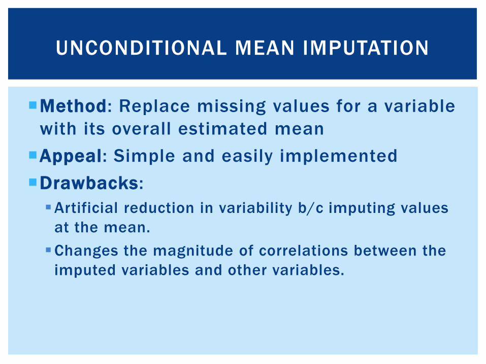
Method: Replace missing values for a variable
with its overall estimated mean
Appeal: Simple and easily implemented
Drawbacks:
Artificial reduction in variability b/c imputing values
at the mean.
Changes the magnitude of correlations between the
imputed variables and other variables.
UNCONDITIONAL MEAN IMPUTATION

MEAN, SD AND CORRELATION MATRIX OF 5 VARIABLES
BEFORE & AFTER MEAN IMPUTATION

Method: Replace missing values with
predicted scores from a regression equation.
Appeal: Uses complete information to impute
values.
Drawback: All predicted values fall directly on
the regression line, decreasing variability.
Also known as regression imputation
SINGLE OR DETERMINISTIC
(REGRESSION) IMPUTATION

SINGLE OR DETERMINISTIC
(REGRESSION) IMPUTATION
p.46, Applied Missing Data Analysis, Craig Enders (2010)

Imputing values directly on the regression
line:
Underestimates uncertainty
Inflates associations between variables because it
imputes perfectly correlated values
Upwardly biases R-squared statistics, even under the
assumption of MCAR
SINGLE OR DETERMINISTIC
(REGRESSION) IMPUTATION

Stochastic imputation addresses these problems
with regression imputation by incorporating or
"adding back" lost variability.
Method: Add randomly drawn residual to imputed
value from regression imputation. Distribution of
residuals based on residual variance from regression
model.
STOCHASTIC IMPUTATION

STOCHASTIC IMPUTATION
p.48, Applied Missing Data Analysis, Craig Enders (2010)

Appeals:
Restores some lost variability.
Superior to the previous methods as it will
produce unbiased coefficient estimates under
MAR.
Drawback: SE’s produced during stochastic
estimation, while less biased, will still be
attenuated.
STOCHASTIC IMPUTATION
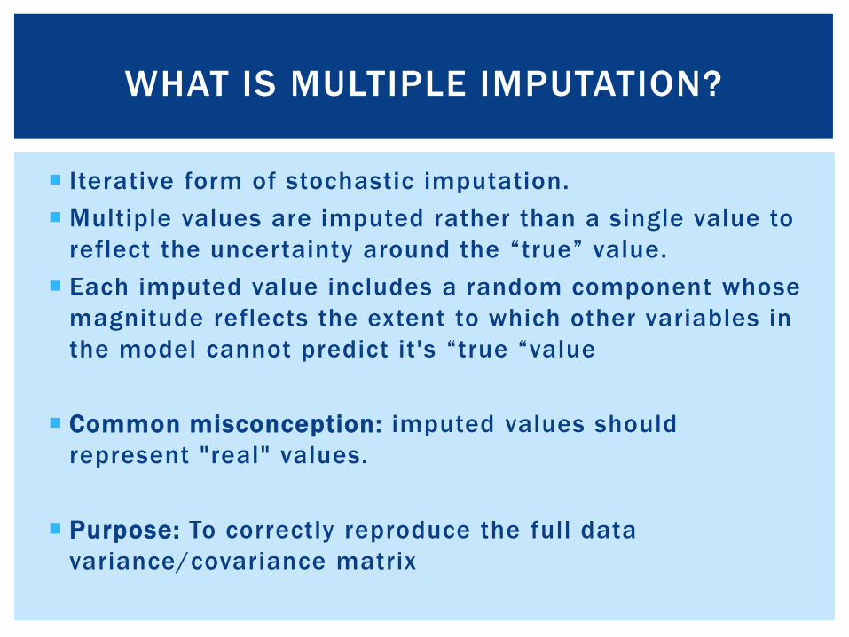
Iterative form of stochastic imputation.
Multiple values are imputed rather than a single value to
reflect the uncertainty around the “true” value.
Each imputed value includes a random component whose
magnitude reflects the extent to which other variables in
the model cannot predict it's “true “value
Common misconception: imputed values should
represent "real" values.
Purpose: To correctly reproduce the full data
variance/covariance matrix
WHAT IS MULTIPLE IMPUTATION?

No.
This is argument applies to single imputation methods
MI analysis methods account for the uncertainty/error
associated with the imputed values.
Estimated parameters never depend on a single value.
ISN'T MULTIPLE IMPUTATION JUST
MAKING UP DATA?
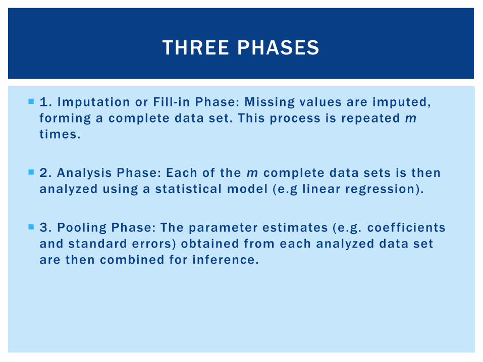
1. Imputation or Fill - in Phase: Missing values are imputed,
forming a complete data set. This process is repeated m
times.
2. Analysis Phase: Each of the m complete data sets is then
analyzed using a statistical model (e.g linear regression).
3. Pooling Phase: The parameter estimates (e.g. coefficients
and standard errors) obtained from each analyzed data set
are then combined for inference.
THREE PHASES

The imputation model should be "congenial“ to or consistent
with your analytic model:
Includes, at the very least, the same variables as the analytic model.
Includes any transformations to variables in the analytic model
E.g. logarithmic and squaring transformations, interaction terms
All relationships between variables should be represented and
estimated simultaneously.
Otherwise, you are imputing values assuming they are
uncorrelated with the variables you did not include.
THE IMPORTANCE OF BEING COMPATIBLE

1. Examine the number and proportion of missing values
among your variables of interest .
2. Examine Missing Data Patterns among your variables of
interest.
3. If necessary, identify potential auxiliary variables
4. Determine imputation method
PREPARING FOR MULTIPLE IMPUTATION

EXAMINE MISSING VALUES: PROC
MEANS NMISS OPTION

EXAMINE MISSING VALUES: NOTE VARIABLE(S ) WITH
HIGH PROPORTION OF MISSING -- THEY WILL IMPACT
MODEL CONVERGENCE THE MOST

proc mi data=hsb_mar nimpute=0 ;
var write read female math prog ;
ods select misspattern;
run;
EXAMINE MISSING DATA PATTERNS:
SYNTAX

EXAMINE MISSING DATA PATTERNS

Characteristics:
Correlated with missing variable (rule of thumb: r> 0.4)
Predictor of missingness
Not of analytic interest, so only used in imputation model
Why? Including auxiliary variables in the imputation model can:
Improve the quality of imputed values
Increase power, especially with high fraction of missing information (FMI >25%)
Be especially important when imputing DV
Increase plausibility of MAR
IDENTIFY POTENTIAL AUXILIARY
VARIABLES

A priori knowledge
Previous literature
Identify associations in data
HOW DO YOU IDENTIFY
AUXILIARY VARIABLES?

AUXILIARY VARIABLES ARE CORRELATED
WITH MISSING VARIABLE

AUXILIARY VARIABLES ARE PREDICTORS
OF MISSINGNESS

IMPUTATION MODEL
EXAMPLE 1:
MI USING MULTIVARIATE
NORMAL DISTRIBUTION
(MVN)

Probably the most common parametric approach for multiple
imputation.
Assumes variables are individually and jointly normally
distributed
Assuming a MVN distribution is robust to violations of
normality given a large enough N.
Uses the data augmentation (DA) algorithm to impute.
Biased estimates may result when N is relatively small and
the fraction of missing information is high.
ASSUMING A JOINT MULTIVARIATE
NORMAL DISTRIBUTION

proc mi data= new nimpute=10 out=mi_mvn seed=54321;
var socst science write read female math progcat1 progcat2 ;
run;
IMPUTATION PHASE

MULTIPLY IMPUTED DATASET

proc glm data = mi_mvn ;model read = write female math progcat1 progcat2;by _imputation_;ods output ParameterEstimates=a_mvn;run;quit;
ANALYSIS PHASE:
ESTIMATE MODEL FOR EACH
IMPUTED DATASET

PARAMETER ESTIMATE DATASET

proc mianalyze parms=a_mvn;
modeleffects intercept write female math
progcat1 progcat2;
run;
POOLING PHASE-
COMBINING PARAMETER ESTIMATES
ACROSS DATASETS


COMPARE MIANALYZE ESTIMATES
TO ANALYSIS WITH FULL DATA
FULL DATA ANALYSIS
MIANALYZE OUPUT

PROC MIANALYZE combines results across imputations
Regression coefficients are averaged across imputations
Standard errors incorporate uncertainty from 2 sources:
"within imputation" - variability in estimate expected with no missing data
The usual uncertainty regarding a regression coefficient
"between imputation" - variability due to missing information.
The uncertainty surrounding missing values
HOW DOES PROC MIANALYZE WORK

OUTPUT FROM MIANALYZE

Sampling variability expected with no missing data.
Average of variability of coefficients within an imputation
Equal to arithmetic mean of sampling variances (SE2)
Example: Add together 10 estimated SE2 for write and divide by10
Vw = 0.006014
VARIANCE WITHIN

Variability in estimates across imputations
i.e. the variance of the mcoefficients
Estimates the additional variation (uncertainty) that results from missing data.
Example: take all 10 of the parameter estimates (β) for write and calculate the variance
VB = 0.000262.
VARIANCE BETWEEN

The total variance is sum of 3 sources of variance.
Within,
Between
Additional source of sampling variance.
What is the sampling variance?
Variance Between divided by number of imputations
Represents sampling error associated with the overall coefficient estimates.
Serves as a correction factor for using a specific number of imputations.
TOTAL VARIANCE

DF for combined results are determined by the number of imputations.
*By default DF = infinity, typically not a problem with large N but can be with smaller samples
The standard formula to estimate DF can yield estimates that are fractional or that far exceed the DF for complete data.
Correction to adjust for the problem of inflated DF has been implemented
Use the EDF option on the proc mianalyze line to indicate to SAS what is the proper adjusted DF.
DEGREES OF FREEDOM
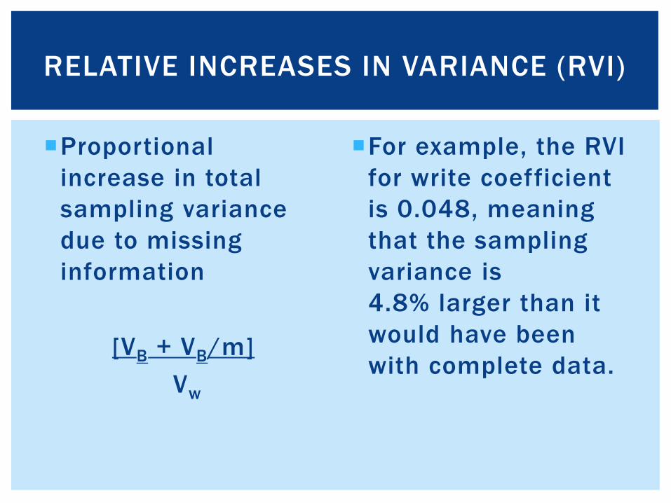
Proportional
increase in total
sampling variance
due to missing
information
[VB + VB/m]
Vw
For example, the RVI
for write coefficient
is 0.048, meaning
that the sampling
variance is
4.8% larger than it
would have been
with complete data.
RELATIVE INCREASES IN VARIANCE (RVI)

Directly related to RVI.
Proportion of total sampling variance that is due to missing data
[VB + VB/m]
VT
For a given variable, FMI based on percentage missing and correlations with other imputation model variables.
Interpretation similar to an R2. Example: FMI=.046 for
write means that 4.6% of sampling variance is attributable to missing data.
FRACTION OF MISSING INFORMATION
(FMI)

Captures how well true population parameters are estimated
Related to both the FMI and m
Low FMI + few m = high efficiency
As FMI increase so should m: Better statistical power and more stable estimate
RELATIVE EFFICIENCY:
IS 5 IMPUTATIONS ENOUGH?

DIAGN0STICS:
HOW DO I KNOW IF IT WORKED?
Compare means and frequencies of observed
and imputed values.
Use boxplots to compare distributions
Look at “Variance Information” tables from
the proc mianalyze output
Plots - Assess convergence of DA algorithm

Convergence for each imputed variable can be
assessed using trace plots.
Examine for each imputed variables
Special attention to variables with a high FMI
proc mi data= ats.hsb_mar nimpute=10
out=mi_mvn;
mcmc plots=trace plots=acf ;
var socst write read female math;
run;
TRACE PLOTS:
DID MY IMPUTATION MODEL CONVERGE?


EXAMPLE OF A POOR TRACE PLOT

Assess possible auto correlation of parameter values between iterations.
Assess the magnitude of the observed dependency of imputed values across iterations.
proc mi data= ats.hsb_mar nimpute=10 out=mi_mvn;mcmc plots=trace plots=acf ;var socst write read female math;run;
AUTOCORRELATION PLOTS:
DID MY IMPUTATION MODEL CONVERGE?


IMPUTATION MODEL
EXAMPLE 2:
MI USING FULLY
CONDITIONAL
SPECIFICATION (FCS)

WHAT IF I DON’T WANT TO ASSUME A
MULTIVARIATE NORMAL DISTRIBUTION?
Alternative method for imputation is Fully Conditional Method (FCS)
FCS does not assume a joint distribution and allows the use of different distributions across variables.
Each variable with missing is allowed its own type of regression (linear, logistic, etc) for imputation
Example uses: Logistic model for binary outcome
Poisson model for count variable
Other bounded values

FCS methods available:
Discriminant function or logistic regression for binary/categorical variables
Linear regression and predictive mean matching for continuous variables.
Properties to Note:
1. Discriminant function only continuous vars as covariates (default).
2. Logistic regression assumes ordering of class variables if more then two levels (default).
3. Regression is default imputation method for continuous vars.
4. PMM will provide “plausible” values.
1. For an observation missing on X, finds cases in data with similar values on other covariates, then randomly selects an X value from those cases
AVAILABLE DISTRIBUTIONS

IMPUTATION PHASE
proc mi data= ats.hsb_mar nimpute=20
out=mi_fcs ;
class female prog;
fcs plots=trace(mean std);
var socst write read female math science prog;
fcs discrim(female prog /classeffects=include)
nbiter =100 ;
run;

proc mi data= ats.hsb_mar nimpute=20
out=mi_new1;
class female prog;
var socst write read female math science prog;
fcs logistic (female= socst science) ;
fcs logistic (prog =math socst /link=glogit)
regpmm(math read write);
run;
ALTERNATE EXAMPLE

proc genmod data=mi_fcs;
class female prog;
model read=write female math prog/dist=normal;
by _imputation_;
ods output ParameterEstimates=gm_fcs;
run;
ANALYSIS PHASE:
ESTIMATE GLM MODEL USING EACH
IMPUTED DATASET


PROC MIANALYZE parms(classvar=level)=gm_fcs;
class female prog;
MODELEFFECTS INTERCEPT write female math
prog;
RUN;
POOLING PHASE-
COMBINING PARAMETER ESTIMATES
ACROSS DATASETS

TRACE PLOTS:
DID MY IMPUTATION MODEL CONVERGE?

FCS HAS SEVERAL PROPERTIES THAT
MAKE IT AN ATTRACTIVE ALTERNATIVE
1. FCS allows each variable to be imputed using its
own conditional distribution
2. Different imputation models can be specified for
different variables. However, this can also cause
estimation problems.
Beware: Convergence Issues such as complete and
quasi-complete separation (e.g. zero cells) when
imputing categorical variables.

MI improves over single imputation methods
because:
Single value never used
Appropriate estimates of uncertainty
The nature of your data and model will
determine if you choose MVN or FCS
Both are state of the art methods for handling
missing data
Produce unbiased estimates assuming MAR
BOTTOM LINE