modeling the impact of a phosphogypsum … modeling the impact of a phosphogypsum stack on the...
TRANSCRIPT

1
MODELING THE IMPACT OF A
PHOSPHOGYPSUM STACK ON THE GROUNDWATER AQUIFER
by
Manfred Koch
and
Takashi Thomas Shinkawa
Temple University
Philadelphia, PA 19122
March, 1997

2
TABLE OF CONTENTS
1. INTRODUCTION………………………………………………
2. BACKGROUND……………………………………………….
Location…………………………………………………….
Geology……………………………………………………..
Hydrogeology………………………………………………
3. METHODS OF DATA ANALYSIS ..…………………………
Phosphogypsum Stack……………………………………
Surficial Aquifer………………………………………….
4. HYDROLOGIC DATA ..………………………………………
Stack Analysis……….……………………………………..
Analysis of Hydraulic Heads………….……………
Cooper-Jacob Straightline Method..…………………
Pressure Transducer Tests …………………………..
Borehole Flowmeter Tests …………………………….
Surficial Aquifer………………………………………….
Regional Flow Trend………………………………….
Water Table Contours……………………………….
Conductivity Analysis………………………………
Kirkham Auger HoleTest……………………
Bouwer Rice Test……………………………..
Precipitation………………………………………………
5. GROUNDWATER FLOW MODEL………………………….
Description of the MODFLOW model…………….
Mathematical Theory
Design of the flow model………………………
The conceptual model
Grid geometry……………………………………..
Hydrologic Parameters…………………………….
Boundary Conditions ……………………………..
3
Sources and Sinks ………………………………..
Calibration……………………………………………….
Sensitivity Analysis………………………………………
Leakance……………………………………………
Conductivities………………………………………
Ditch Specifications………………………………..
Water Budget Analysis…………………………………..
6. CONCLUSIONS……………………………………………
REFERENCES CITED………………………………………….
APPENDICES……………………………………………………….
I: Cooper-Jacob Straightline Plots
II: Pressure Transducer Tests
III: Hydraulic Head Contour Plots
IV: Bouwer Rice Plots

4
CHAPTER 1
INTRODUCTION
Phosphate mining in Florida is currently one of the state’s largest industries, and
produces approximately 40 million tons of material per year (Miller and Sutcliffe, 1984).
Estimates from previous studies indicate that 335 million tons of phosphatic waste have
been stockpiled in above-ground formations called “Phosphogypsum Stacks” (defined as
such by the source and product of their existence). Gypsum and silicon hexafluoride make
up the slimy waste that is pumped out to large evaporite ponds, where the former is
allowed to precipitate. Over time, accumulation at the bottom of the pond is dug out and
piled on the embankments of the pond. This practice is intended to strengthen the walls of
the pond, as it grows in size and elevation. Approximately eighteen such industrial
facilities are located in the Tampa area, with an average area of 227 acres and a range of
heights between 30 and 140 feet.
As the stockpile of gypsum stacks grow to a projected billion-plus tons by the year
2000 (May and Sweeney, 1983), the high concentrations of radionuclides, acid, fluoride,
phosphate, and sulfate become an increasingly problematic characteristic of this
resource, with the potential for groundwater pollution.
The primary focus of this study was to investigate the hydrologic controls of the
phosphogypsum stack, and to provide a model of groundwater flux upon which a future
transport and geochemical model can determine the migration and fate of possible
contaminant leachate plumes and to delineate the physical and chemical processes
involved. As to the more particular objectives of the hydrological part of the research

5
they amount to a quantification of the vertical and horizontal flow rates in the
phosphogypsum stack and the surficial aquifer, respectively, as well as to a
determination of the hydraulic impact of the phosphogypsum stack on the surficial
aquifer.
6
CHAPTER 2
ENVIRONMENTAL SETTING
Geography
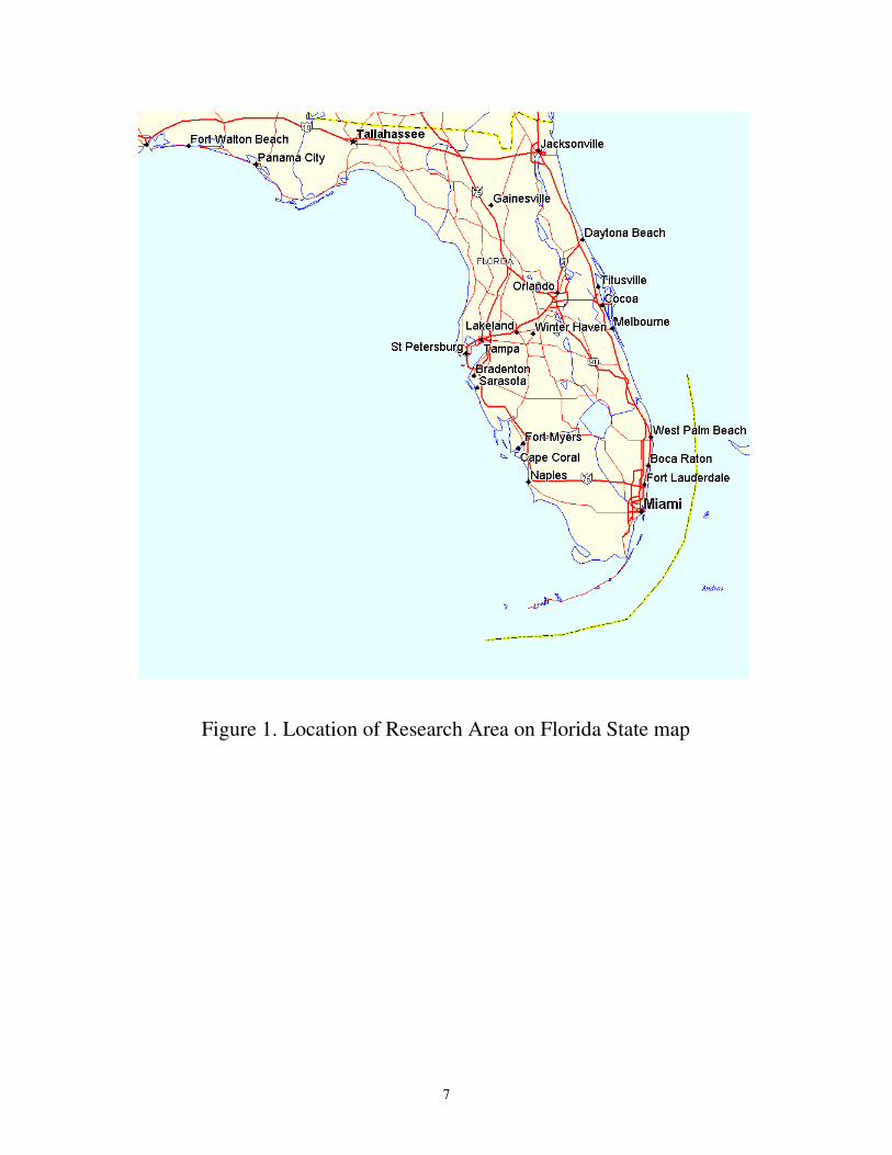
The Piney Point Phosphates facility, located along the coast of western Florida,
lies approximately 30 kilometers south of downtown Tampa in Manatee County, along
Florida route 41 (figure 1). The study area is a rural setting with cattle ranches, citrus
groves, and vegetable farms making up a majority of the businesses close by.
Topographically, the area is relatively flat with drainage flowing either to the Manatee
River in the North, McMullen Creek in the South, or to the Gulf of Mexico in the West
(figure 2). The Piney Point Phosphates complex is at an elevation of 3 - 8 m. above mean
sea level, and is about two kilometers from the shoreline of the Gulf of Mexico.
The climate of the research area is subtropical. Convective thunderstorms
dominate the rainy weather of the summer months, while winter and spring are fairly dry.
Consequently, irrigation demands on the groundwater reach a peak from March through
May.
This particular site, although presently inactive, is an ideal location for studying
fluid migration from phosphogypsum stacks, owing to the fact that local groundwater
movement is toward the Gulf of Mexico and away from any large population in the area.
Major lithologies of stratigraphic units in the area define three distinct groups of
formations (figure 3). Each groups bears significance as a water producing unit with
respective hydrologic importance to its defining lithology. Although heterogeneous
7
Figure 1. Location of Research Area on Florida State map

8
Sho
relin
e
5
10
15 20
25
30
35
0 1 2 km.
SCALELEGEND
Piney Point Complex
Roads
Waterways
5
35
10
35
10
25
30
30
25
20
510
15
20
GULF of MEXICO
Figure 2. Topographical map of Research Area. Data has been taken
from USGS 7.5 -minute maps using 5 foot contour intervals.

9
characterization of lithologies within each group exist (table 1), generalization of the
groups’ defining units will be the limit to which the investigation is concerned.
The base of the stratigraphic column (figure 3) is made up of the Suwanee, Ocala,
and Avon Park Limestones. Together, these formations comprise a 150 - 250 m thick
limestone unit which is commonly referred to as the Floridian Aquifer. Boundaries of this
limestone group are defined beneath by a carbonate unit containing intergranular
evaporites, and above by another carbonate unit with higher percentages of clays (Miller
and Sutcliffe, 1984).
Overlying the Floridian Aquifer are alternating sandy limestone and clay layers.
This alternation of layers is classified as a second lithological group, and is composed of
the Tampa and Hawthorn Formations. Although this intermediate group can be used as a
source of water, it is primarily made of various clays. The upper confine of the unit is
delineated by a phosphatic clay, known as the Bone Valley Formation. It is used as the
ore for the phosphate industry in the area and has been called “one of the world’s most
important sources of phosphate” (Miller and Sutcliffe, 1984). Thickness of the
intermediate unit is from 75 - 125 m , with the phosphatic clay composing the upper 10 -
20 m.
At the surface, a 10-20 m thick unit of undifferentiated sands and clays is
classified as the third lithological group of this section of the stratigraphy. It consists
primarily of surficial sands with occasional clay lenses, and is lithologically distinct from
the other two units.

10
Figure 3. Stratigraphic Cross Section of Regional Geology
A Generalized Lithological Representation of Stratigraphic Units
below Piney Point Phosphates, INC.

11
Table 1. Stratigraphic Framework (Miller and Sutcliffe, 1984)
System
Series
Stratigraphic
Unit
General
Lithology
Major
Lithological
Unit
Hydrogeologic
Unit
Quaternary Holocene,
Pleistocene
Surficial
Sand, terrace
sand,
phosphorite
Predominantly fine
sand; interbedded
clay, marl, shell,
limestone,
phosphorite
Sand Surficial Aquifer
Pliocene Bone Valley
Formation
Clayey and Pebbly
Sand; clay, marl,
shell, phosphatic
Phosphatic
Clay
Confining unit
Hawthorn
Formation
Dolomite, sand,
clay, and
limestone; silty,
phosphatic
Carbonate
and Clastic
Intermediate
Aquifer system
(Includes First
and Second
Aquifers)
Miocene Tampa
Limestone
Limestone, sandy,
phosphatic,
fossiliferous; sand
and clay in lower
part in some areas
Tertiary Oligocene Suwanee
Limestone
Limestone, sandy
limestone,
fossiliferous
Ocala
Limestone
Limestone, chalky,
foraminiferal,
dolomitic near
bottom
Carbonate
Floridan Aquifer
Eocene,
Paleocene
Avon Park
limestone
Limestone and hard
brown dolomite
Lake City,
Oldsmar, and
Cedar Key
Limestones
Dolomite and
chalky limestone,
with intergranular
gypsum and
anhydrite
Carbonate
w/
intergranular
evaporites
lower confining
bed of floridan
aquifer

12
Hydrogeology
Groundwater in the area is commonly drawn from one of the three available water
producing units described above. Flow within these aquifers is, for the most part, in the
horizontal direction with little leakage between layers. The water table in the unconfined
unit varies with precipitation and evaporation, while underlying units modulate their
potentiometric yields according to changing lateral flow from inland areas of recharge
and local points of discharge. Seasonal highs and lows of the potentiometric surfaces
have been recognized by the U.S. Geological survey (Johnson et. al., 1981) as September
and May, respectively, and are mainly associated with groundwater pumpage for
agricultural irrigation.
Comparison of the potentiometric surfaces in the southeastern United States by
Johnston et.al. (1980,1981) before and after development has shown a regional trend in
the vertical flow between aquifer units. Following extensive development of the area in
the late 1970’s, Polk County to the East had become an area of recharge whereas the
coastal area along Tampa Bay had become a zone of discharge to the Gulf of Mexico.
This trend dictates a downward flow to the Floridan Aquifer in the area of recharge, and
an upward flow in the area of discharge. Because the Piney Point facility is in the area of
discharge, there exists an upward flow gradient in the water-bearing units through their
confining beds.
Locally, groundwater is drawn primarily from the Floridan Aquifer, although the
surficial and intermediate aquifers are equally important to some. The surficial unit is
used for domestic lawn irrigation, while the intermediate aquifer system is tapped for use
as a rural domestic source of water and for agricultural irrigation. Additionally, the

13
Floridan aquifer south of the Piney Point facility contains mineralized water, and
promotes the intermediate aquifer as the primary source for municipal water.
In the studies of Miller and Sutcliffe (1982) and Miller and Sutcliffe (1984) the
aquifer system around the Piney Point complex was probed for the first time in more
detail. About forty test holes (wells) whose depths extended from the surficial,
unconfined aquifer to the intermediate, confined (artesian) aquifer were drilled around the
ponds and the gypsum stack during this study. A few older, mostly abandoned irrigation
wells that extend further down into the confined Floridan aquifer were also monitored.
Various geophysical well-logging techniques were applied in some of the boreholes to
determine the lithology of the aquifer substratum. Groundwater table elevations were
taken data during the time and three wells were monitored continuously by means of
recorders. The hydrographs for the three continuously monitored wells show sporadic
evidence of an upward hydraulic head gradient between the intermediate and the surficial
aquifer. This has been taken as evidence that potential surface contamination cannot leak
into the lower intermediate aquifer. However, during the dry season (April to June), when
the intermediate aquifer is heavily pumped for agricultural irrigation, the situation may be
reversed and a downward gradient is observed. The water elevation data shows also a
topographic mounding effect of the gypsum stack on the groundwater-level in the
surficial aquifer.
The Piney Point Phosphate Inc.'s quarterly reports of the groundwater monitoring
survey around the phosphogypsum stack to the Florida Department of Environmental
Protection (FDEP) provide some evidence of the direction of the regional groundwater
flow in the vicinity of the stack. As part of the proposed extension of the phosphogypsum

14
stack to its present-day size, Gerathy & Miller Inc. was consulted by the Piney Point Inc.
to install 7 monitor wells extending into the surficial aquifer on the premises of the
company. Most of these monitor wells are still in use today and are being sampled on a
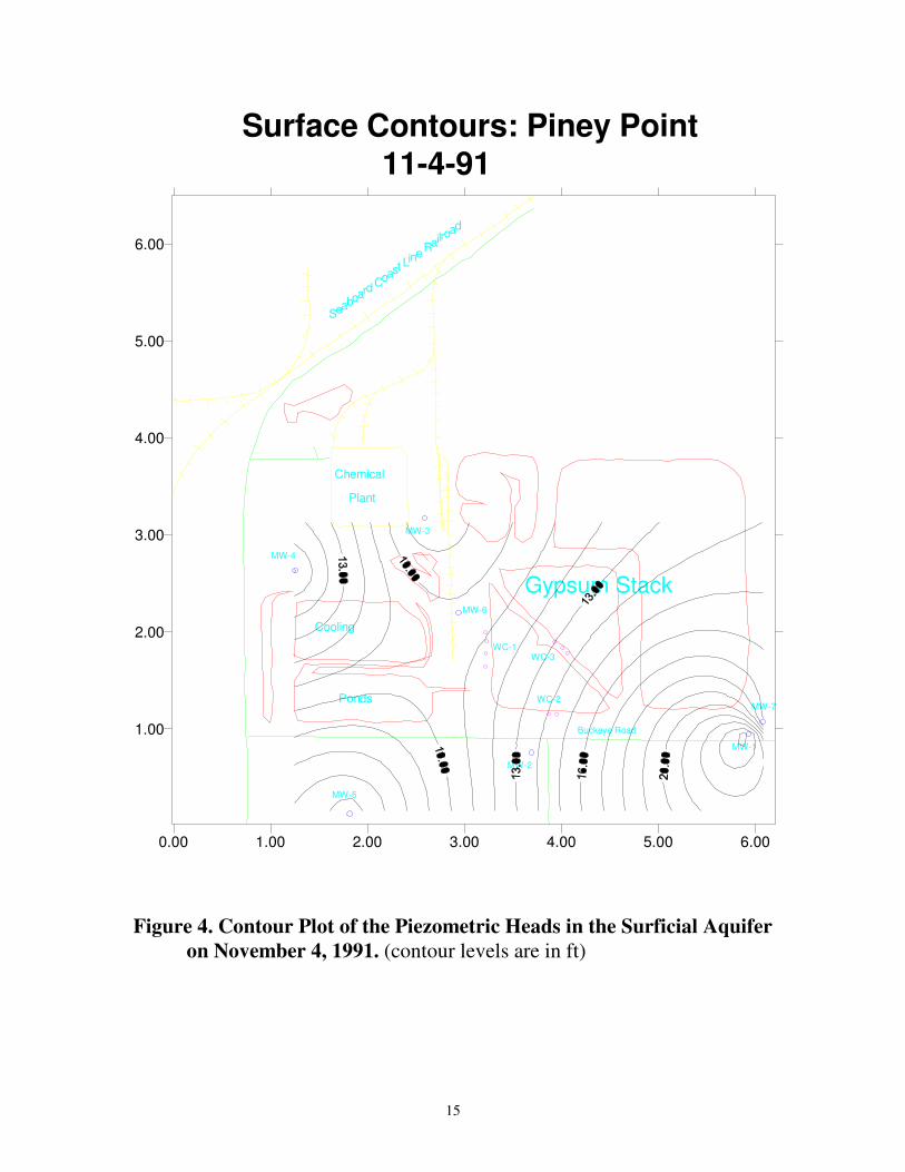
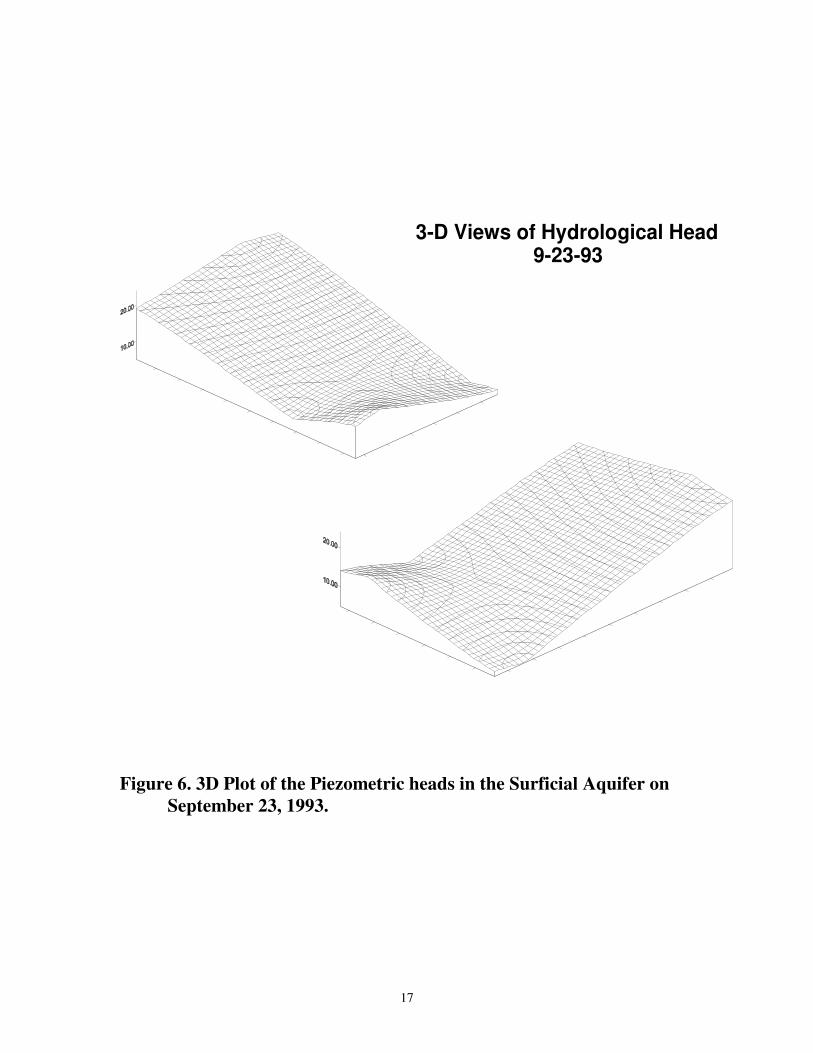
regular basis. Figures 4 and 5 show the piezometric isolines for two particular dates and
Figure 6 illustrates the hydraulic head surface for one of these dates in 3D form. One can
observe from these figures that the groundwater flow is mainly in northwestern direction.
Moreover, the flow system in the surficial aquifer appears to be very much in steady-
state, as witnessed by the similarity of the isoline contours taken two years.
As for the hydrogeology in the phosphogypsum stack itself, only the geotechnical
study of the slope stability carried out by Oaks Geotechnical Inc. (1980) as part of the
proposed extension of the gypsum stack to its present-day size provides some
rudimentary clues about the water flow in the stack. During this study several boreholes
were drilled into the flanks of the stack and water-table levels were monitored over a
period of several months. Because the exact well construction data has not been reported
precise inferences on the stack-flow cannot be made.
15
Gypsum Stack
Buckeye Road
Chemical
Plant
SeaboardCoast
LineRailro
ad
Cooling
Ponds
MW-1
MW-7
MW-5
MW-2
MW-6
MW-4
MW-3
WC-3WC-1
WC-2
0.00 1.00 2.00 3.00 4.00 5.00 6.00
1.00
2.00
3.00
4.00
5.00
6.00
Surface Contours: Piney Point 11-4-91
Figure 4. Contour Plot of the Piezometric Heads in the Surficial Aquifer
on November 4, 1991. (contour levels are in ft)

16
Gypsum Stack
Buckeye Road
Chemical
Plant
Seaboard C
oast Line R
ailroad
Cooling
Ponds
MW-1
MW-7
MW-5
MW-2
MW-6
MW-4
MW-3
WC-3WC-1
WC-2
0.00 1.00 2.00 3.00 4.00 5.00 6.00
1.00
2.00
3.00
4.00
5.00
6.00
Surface Contours: Piney Point 9-23-93
Figure 5. Contour Plot of the Piezometric heads in the Surficial Aquifer
on September 23, 1993. (contour levels are in ft)
17
3-D Views of Hydrological Head 9-23-93
Figure 6. 3D Plot of the Piezometric heads in the Surficial Aquifer on
September 23, 1993.

18
CHAPTER 3
METHODS OF DATA ANALYSIS
Compilation of the data as well as computation for the analyses was conducted in
spreadsheet format using Microsoft Excel. Representation of this data as graphs, in
addition to a regression for the topographical analysis were done in Axum 5.0.
Modification of some figures was accomplished through use of Microsoft Paint, and
Hijaak Pro.
Phosphogypsum Stack
Identification of hydrologic flow within the phosphogypsum pile itself was carried
out through a series of investigations centered around quantifying the hydrologic
parameters of the stack material, and identifying vertical gradients between stratigraphic
layers. Ten partially screened wells and one fully screened well were drilled into the
oldest portion of the stack. The wells were set at various depths (Table 2) in two clusters
of four wells and one cluster of three. Cluster one (PP1) in the west wall and cluster three
(PP3) in the center of the stack along an old working road wall had four wells, while
cluster two (PP2) in the south wall only had three wells (figure 7). The gypsum-aquifer
interface (base of the stack) is at a depth of 20.8 m from the surface, so there is only one
well which taps the surficial aquifer through the gypsum stack

19
00 300300 600600
Seaboard C
oast Line R
ailroad
Seaboard C
oast Line R
ailroad
82 32’82 32’
LakeLake
CoolingCooling
PondsPonds
Buckeye RoadBuckeye Road
55 22
S2
4A4A
38’38’R1
33
CHEMICALCHEMICAL
PLANTPLANT
R2
N
1616 1515
1717
99
10101111
1212
1414
39 39
33
3838 3737
1313
2727OO
41
1818 1919
2020
2121
2222
2424
2323
S1
New PhosphogypsumNew Phosphogypsum
Ponds Ponds
88 11
77
3636
3434
2323
Old Old
PhosphogypsumPhosphogypsum
PondsPonds
Figure 7 - Locations of Monitoring Wells at Figure 7 - Locations of Monitoring Wells at Piney Point Phosphates, Inc. Palmetto, FloridaPiney Point Phosphates, Inc. Palmetto, Florida
DIAMMONIUMDIAMMONIUM
PHOSPHATEPHOSPHATE
PONDPOND
Scale (meters)Scale (meters)
9, 10, 119, 10, 11
Research WellsResearch Wells
Surface Sample SiteSurface Sample Site
Rainfall Sample SiteRainfall Sample Site
Old PiezometersOld Piezometers
PG Stack WellsPG Stack Wells
LegendLegend
USGS WellsUSGS Wells
00
Monitor WellsMonitor Wells
(AMAX)(AMAX)
88
TT
UU
KK JJ
110110
131315156a6a
99
1010
1111

20
Table 2 - Depths of Sampling Wells Drilled into the Stack
Cluster # - Well #
Total Well Depth
(in m. from top of
riser)
Cased
Section
(m. depth)
Screened
Section
(m. depth)
1 - 1 18.0 0 - 14.8 14.8 - 18
1 - 2 14.8 0 - 12.5 12.5 - 14.8
1 - 3 12.5 0 - 9.5 9.5 - 12.5
1 - 4 9.5 0 - 6.6 6.6 - 9.5
2 - 0 23.6 0 - 22.0 22.0 - 23.6
2 - 1 18.0 0 - 14.8 14.8 - 18.0
2 - 2 14.8 0 - 12.5 12.5 - 14.8
2 - 3 11.5 0 - 8.2 8.2 - 11.5
3 - 1 18.0 none 0 - 18.0
3 - 2 14.8 0 - 12.5 12.5 - 14.8
3 - 3 11.5 0 - 8.2 8.2 - 11.5
All wells were constructed with a 10 cm. diameter PVC pipe. Screens were
packed in 20-30 mesh sand with approximately 50 cm of bentonite hole plug overlying
the sand pack except for the PP 2-0 well which has a 2m thick bentonite plug over the
sand pack. The risers were grouted to the surface with a bentonite-cement mixed grout
compound. For the fully screened well PP 3-0 grout-plugs were set at intervals of 1.5m,
in order to reduce the possibility of vertical outer-borehole flow which could corrupt the
borehole flowmeter tests.
Quantification of hydrologic parameters within the stack was determined by one
of the most commonly used non-equilibrium pump tests, the Cooper-Jacob (straight-line)
method. This method was used over the more popular Theis-curve match for its
asymptotic approximation of the well function for a small radius and long times, because
21
it is important to rule out the bias of values representative of the region directly around
the well. A Grundfos 1.2-amp pump was used to pump water out of the well at an
approximate rate of 6 L/min., and head measurements were taken with an electrical head
level indicator.
Hydraulic gradients within the stack were determined by using a pressure
transducer, a new electromagnetic borehole flowmeter (Molz et al., 1994) , and through a
comparison of hydraulic head values. Due to the significance of a hydrologic gradient for
the understanding of the flow system in the stack, the use of these different methods
should increase the reliability of the results obtained.
In situ vertical head measurements were made using a set of inflatable packers
bought from the Tennessee Valley Authority, and a 20 psi pressure transducer from Telog
Instruments, INC. Inflation of the packers above and below the pressure transducer
allowed a section of the well to be isolated, and a reading to be taken. Measurements of
the in situ pressure were taken at all screened intervals possible, along with 3 - 5 cased
intervals (to provide a standard hydrostatic gradient upon which to compare the screened
readings). Variations of anomalous readings in the screened sections were correlated with
the presence of a pressure perturbation (i.e., a flow gradient).
Borehole flowmeter tests were conducted by Quantum Engineering Corporation
using the deepest well of each stack cluster. Ambient flow, induced flow, and pump test
measurements were conducted at all wells; however, a complete analysis was only done
for well 1-1. Results for wells 2-1 and 3-1 were incomplete, owing to the onset of a
thunderstorm the day that the measurements were taken. Results from this testing have
provided data for ambient flow direction and magnitude, as well as response of various

22
vertical sections of the stack to induced flow conditions. Utilization of these induced flow
rates with the measurements for net flow can also be used
Hydraulic head measurements for the monitoring wells on the stack were taken
approximately every three months. Because wells in the same cluster were fairly close
together, comparison of the head measurements were used to indicate possible variations
of head gradients in the vertical direction within the stack. Organization of the data as a
cross-sectional view provided information on internal stack-stratification.
Surficial Aquifer
Analysis of the hydrology in the surficial aquifer includes calculations of
hydraulic conductivities and transmissivities, a contour analysis of monitoring well head
levels, and regional flow gradients in the surficial aquifer. Primary interest of this
research was to quantify horizontal flow rates in the surficial aquifer, as well as to
establish the direction of flow in an attempt to determine the hydraulic impact of the
phosphogypsum stack on the surficial aquifer.
Hydraulic conductivity analyses were conducted by two different analytical
methods, allowing for respective well geometries that were available. USGS well #9
(figure 7) was treated as an auger hole, while all other research wells were drilled to be
partially screened for their lowest 10 feet.
The hydraulic conductivity for the auger hole was calculated according to a
method prescribed by Boast and Kirkham (1971). The well was pumped out by a Grunfos
machine, and the water table (i.e. head) allowed to rebound over the next hour.

23
Measurements of the rebounding head elevation were taken with a conductive measuring
tape, and entered into in a spreadsheet calculation program.
The analysis for the partially penetrating monitor wells was conducted on
proprietary wells 1 and 8, and research wells 11, 18, 21, 22, and 24, using a method
described by Bouwer and Rice (1976). A volume of approximately 200 liters was pumped
out of each well using a Grunfos machine, and then the well was allowed to recharge. As
the hydraulic head rebounded, elevation measurements were taken and imported into a
spreadsheet program.
The contours of the water table on site were compiled every three months using
hydraulic head elevations taken from the following wells : proprietary wells 1 - 5, 8-11,
research wells 8 - 24, U.S.G.S. wells 8, 9, 34, 36, 37, 39, and stack well 2 - 0. Data files
were entered into the Surfer program, and contours generated using the Kriging method.
Because of the importance of the head measurement at well 2-0 (which wasn’t drilled
until March 1996), only contours for months that include measurements at this well are
presented.
The regional flow of the surficial aquifer is partly controlled by the confining unit
beneath it, and its direction and gradient was estimated through an assumption of a
consistent surficial aquifer thickness. Because of a lack of monitor wells further away
from the phosphogypsum stack that would have allowed to properly define the
groundwater gradient the standard assumption was made that the regional flow in the
surficial aquifer is primarily determined by the topographic slope of the land surface. To
determine the latter a three-dimensional regression of the drainage basin using an
equidistant node grid of elevations was made, leading to a first-order representation of the
24
regional flow without the mounding effect of the phosphogypsum stack.. Calculations of
the topographic plane were made in the AXUM graphing program using a collection of
data points taken from topographical maps of the area (figure 3). The transects for the
data point collection were made at a one unit interval (representing 200 m.) of plotted
data in an AutoCAD drawing.
The precipitation for the area was measured daily at stations on site, and at the
U.S.G.S. stations in Ruskin (10 miles to the north), and Bradenton (5 miles to the south).
These data were compared to monitoring well heads and stack pond levels in hydrograph
format. In addition, these hydrographs were analyzed for temporal and spatial relevance
to the possible recharge of the aquifer and the phosphogypsum stack..

25
CHAPTER 4
CHARACTERIZATION OF THE HYDROLOGICAL ENVIRONMENT
This chapter presents the results of the hydrologic characterization of the gypsum
stack and the underlying surficial aquifer, including an analysis of the regional
precipitation data. These characterizations are necessary for the parameter adjustments of
the groundwater model presented in the following chapter. Data are presented in
Appendices I, II, and III.
Stack Analysis
Analysis of Hydraulic Heads
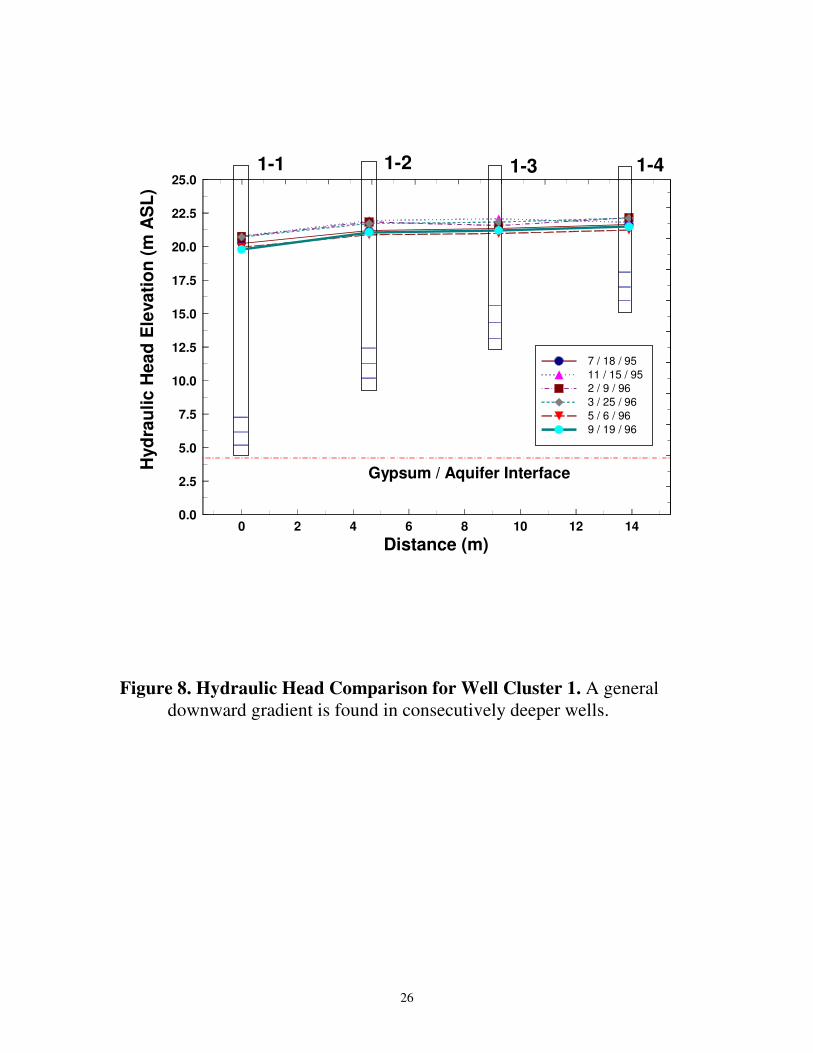
Hydraulic head measurements for all three well clusters demonstrate a downward
flow in all instances. Specific gradients between stratigraphic layers of the gypsum stack
can be made for each of the well regions, as well as a determination of the flow gradient
to the surficial aquifer. Patterns of relative head do not change over time, but can be
correlated to the precipitation record (presented at the end of this chapter).
Well cluster 1 (figure 8) shows a typical illustration of gradualized downward
flow. The occurrence of a slight plateau between wells 1-2 and 1-3 points to a region of
slower flow when compared to the neighboring head gradients to wells 1-1 and 1-4.
Well cluster 3 (figure 9) illustrates flow toward the screening depth of well 3-2,
which is conceptually consistent with well cluster 1, because even though well 3-1 is the
deepest of the three wells, it is fully screened. Thus, head measurements are responding
26
0 2 4 6 8 10 12 14
Distance (m)
0.0
2.5
5.0
7.5
10.0
12.5
15.0
17.5
20.0
22.5
25.0
Hyd
rau
lic
Hea
d E
leva
tio
n (
m A
SL
)
7 / 18 / 95
11 / 15 / 95
2 / 9 / 96
3 / 25 / 96
5 / 6 / 96
9 / 19 / 96
1-1 1-2 1-3 1-4
Gypsum / Aquifer Interface
Figure 8. Hydraulic Head Comparison for Well Cluster 1. A general
downward gradient is found in consecutively deeper wells.

27
0 1 2 3 4 5 6 7 8 9 10 11
Distance (m)
0.0
2.5
5.0
7.5
10.0
12.5
15.0
17.5
20.0
22.5
25.0H
yd
rau
lic H
ead
Ele
va
tio
n (
m M
SL
)
7 / 18 / 95
11 / 15 / 95
2 / 9 / 96
3 / 25 / 96
5 / 6 / 96
5 / 26 / 96
9 / 19 / 96
Gypsum / Aquifer Interface
3-1 3-2 3-3
Figure 9. Hydraulic Head Comparison for Well Cluster 3. A
downward gradient is found toward well 3-2, which represents a head
level for the deepest section of screening in the gypsum stack.
according to their highest screened elevations and force downward flow gradients
between all wells.
28
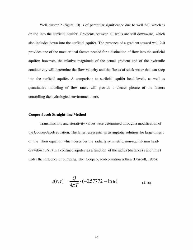
Well cluster 2 (figure 10) is of particular significance due to well 2-0, which is
drilled into the surficial aquifer. Gradients between all wells are still downward, which
also includes down into the surficial aquifer. The presence of a gradient toward well 2-0
provides one of the most critical factors needed for a distinction of flow into the surficial
aquifer; however, the relative magnitude of the actual gradient and of the hydraulic
conductivity will determine the flow velocity and the fluxes of stack water that can seep
into the surficial aquifer. A comparison to surficial aquifer head levels, as well as
quantitative modeling of flow rates, will provide a clearer picture of the factors
controlling the hydrological environment here.
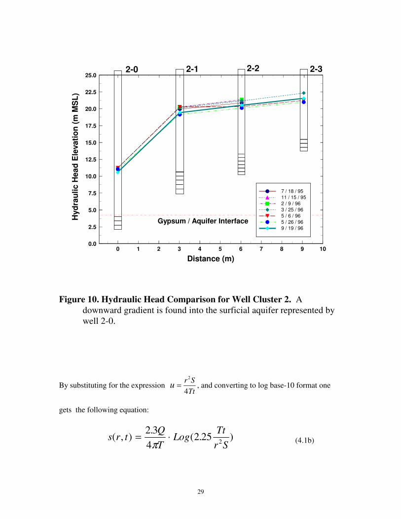
Cooper-Jacob Straight-line Method
Transmissivity and storativity values were determined through a modification of
the Cooper-Jacob equation. The latter represents an asymptotic solution for large times t
of the Theis equation which describes the radially symmetric, non-equilibrium head-
drawdown s(r,t) in a confined aquifer as a function of the radius (distance) r and time t
under the influence of pumping. The Cooper-Jacob equation is then (Driscoll, 1986):
s r tQ
Tu( , ) ( . ln )= ⋅ − −
40 57772
π (4.1a)
29
0 1 2 3 4 5 6 7 8 9 10
Distance (m)
0.0
2.5
5.0
7.5
10.0
12.5
15.0
17.5
20.0
22.5
25.0H
yd
rau
lic H
ea
d E
levati
on
(m
MS
L)
7 / 18 / 95
11 / 15 / 95
2 / 9 / 96
3 / 25 / 96
5 / 6 / 96
5 / 26 / 96
9 / 19 / 96
2-0 2-1 2-2 2-3
Gypsum / Aquifer Interface
Figure 10. Hydraulic Head Comparison for Well Cluster 2. A
downward gradient is found into the surficial aquifer represented by
well 2-0.
By substituting for the expression ur S
Tt=
2
4, and converting to log base-10 format one
gets the following equation:
s r tQ
TLog
Tt
r S( , )
.( . )= ⋅
2 3
42 25
2π
(4.1b)
30
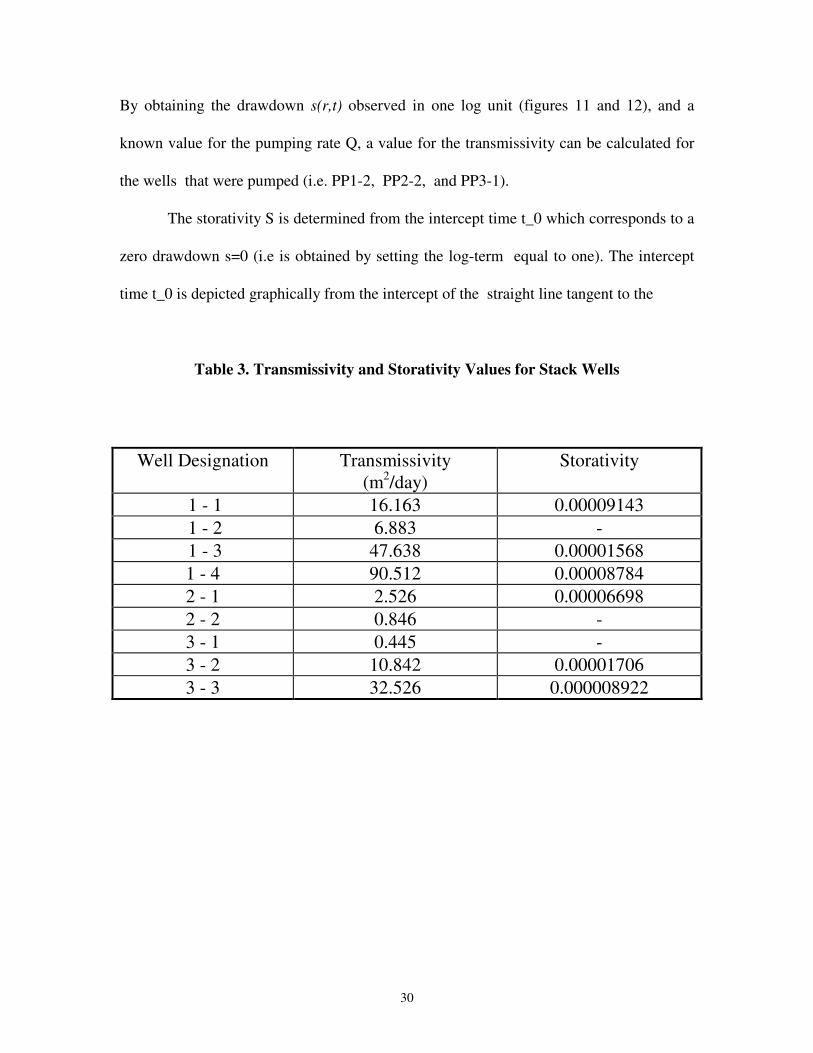
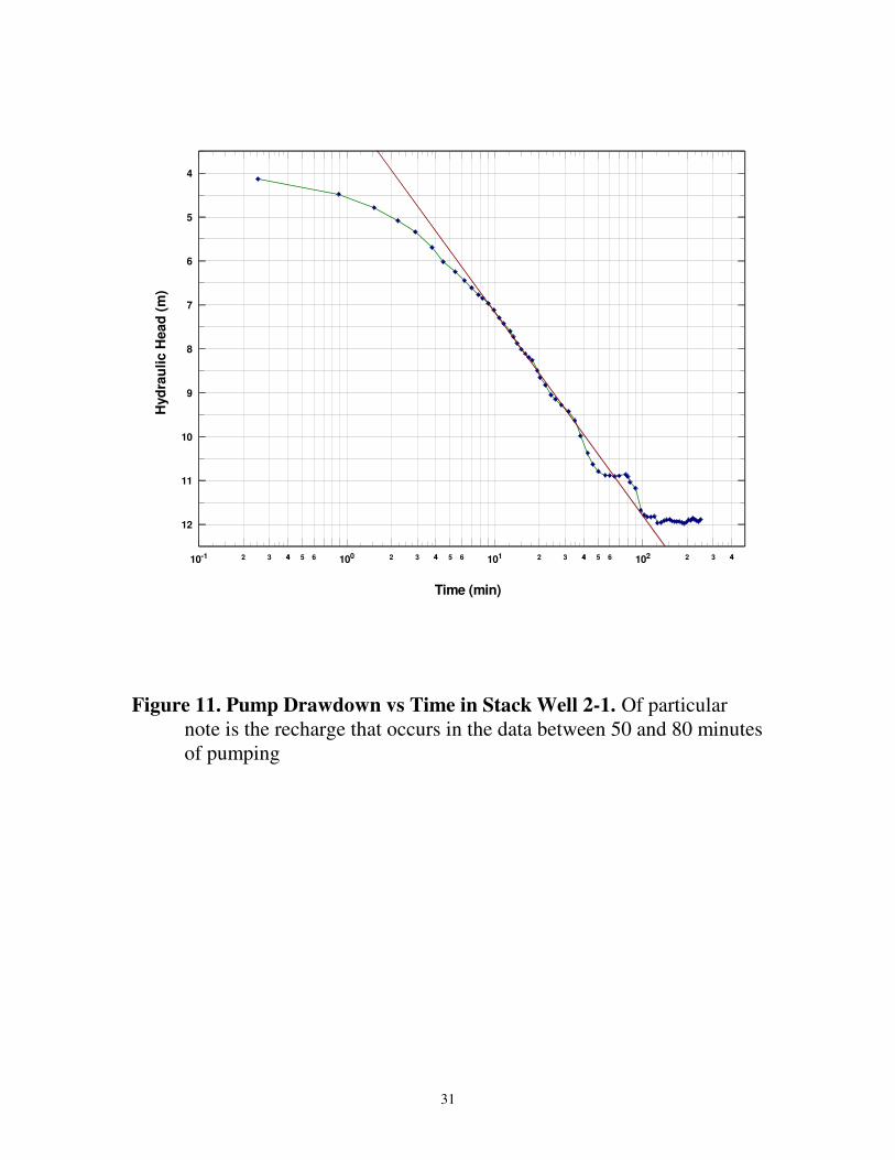
By obtaining the drawdown s(r,t) observed in one log unit (figures 11 and 12), and a
known value for the pumping rate Q, a value for the transmissivity can be calculated for
the wells that were pumped (i.e. PP1-2, PP2-2, and PP3-1).
The storativity S is determined from the intercept time t_0 which corresponds to a
zero drawdown s=0 (i.e is obtained by setting the log-term equal to one). The intercept
time t_0 is depicted graphically from the intercept of the straight line tangent to the
Table 3. Transmissivity and Storativity Values for Stack Wells
Well Designation Transmissivity
(m2/day)
Storativity
1 - 1 16.163 0.00009143
1 - 2 6.883 -
1 - 3 47.638 0.00001568
1 - 4 90.512 0.00008784
2 - 1 2.526 0.00006698
2 - 2 0.846 -
3 - 1 0.445 -
3 - 2 10.842 0.00001706
3 - 3 32.526 0.000008922
31
10-1 2 3 44 5 6 100 2 3 44 5 6 101 2 3 44 5 6 102 2 3 44
Time (min)
12
11
10
9
8
7
6
5
4H
yd
rau
lic
Head
(m
)
Figure 11. Pump Drawdown vs Time in Stack Well 2-1. Of particular
note is the recharge that occurs in the data between 50 and 80 minutes
of pumping

32
2 3 4 55 6 100 2 3 4 55 6 101 2 3 4 55 6 102 2 3 4
Time (min)
6.8
6.6
6.4
6.2
6.0
5.8
5.6
5.4
5.2
5.0
Hyd
rau
lic
He
ad
(m
)
Figure 12. Pump Drawdown vs Time in Stack Well 2-2. Of particular
note is the recharge that occurs in the data between 65 and 90 minutes
of pumping.
33
drawdown curve with the horizontal axis. Values for the storativity S cannot be
determined for the wells that were pumped, since there is a singularity in the solution for r
=0.
Even though transmissivity values for only three of the stack wells were obtained
(Table 3), the wide range found indicates a variation of the transmissivity throughout the
stack. This variation may be caused by modification of the stack structure during
structural maintenance of the stack, whereby gypsum material from the pond is dug out to
strengthen the confining walls. The transmissivity value for well 3-1 is the best
representation of conductivity for the stack as an entire unit (owing to the well’s
representative screened length), while the values for wells 1-2 and 2-2 are more indicative
of particular horizons within the stack.
Storativity values are well constrained, with all values falling within one log unit.
An average of 4.8 x 10⁻⁵ denotes a value comparable to that of natural gypsum,
indicating that the waste material maintains storage properties similar to that of its
chemically related compound.
Although drawdown curves for most of the analyses are typical of a normal
aquifer response, wells 2-1 (figure 11) and 2-2 (figure 12) demonstrate a plateau in their
data close to the equilibrium stage of pumping. This occurrence has been classified as an
influence of recharge, resulting from a proximity to the stack pond. Additionally, the
delay observed between the wells is attributed to the recharge occurring closer to the
pump source. On the other hand, the plateau at well 2-2 is less dramatic because it is on
the perimeter of the drawdown influence.

34
Pressure Transducer Tests
Investigation with the pressure transducer was intended to provide an
identification of horizontal flow within the stack interior. Complete analysis of the
pressure at every depth in all three cluster areas was not possible because of the limited
range provided in the screened sections. Regardless of this restriction, anomalous
horizontal flow was identified in three of the wells. Wells 1-3 (figure 13) and 3-
1 (figure 14) illustrate sections of decreased ambient pressure, while well 3-2 (figure
15) demonstrates a single section of increased pressure. All other wells showed no
deviation from the hydrostatic reference pressure, as computed from the density of the
gypsum stack-water solution, indicating no significant vertical variations of the pressure
and the hydraulic heads in those depths. This means that either there is no significant
amount of vertical flow in that depth-section of the stack that would lead to a detectable
amount of vertical pressure head gradient, or the pressure transducer is just not sensitive
enough to pick it up.
The low pressure zone found at well 1-3 is on the west wall indicating the
presence of a vertical flow gradient at depths approximately 10 m below the surface.
Analysis of well 2-1 examines the same interval on the south wall, but does not indicate
flow different from the expected hydrostatic reference. Thus, no support for a conclusive
statement on the stack edges can be made, but the possibility for flow still exists.
Measurements made at well 3-1 were conducted in a different manner, owing to
the fully screened section of the well. Comparison to unpacked pressure readings instead

35
0 2 4 6 8 10 12 14
Pressure (PSI)
14
12
10
8
6
4
2
De
pth
be
low
Wa
ter
Ta
ble
(m
)Well 1-3
Hydrostatic Norm
Cased Section
Screened Section
Figure 13. Pressure Transducer Measurements for Well 1-3. Deviation
of readings in the screened section (9.5 - 12.5 m.) below the
hydrostatic norm show a regional decrease in ambient pressure.
36
0 2 4 6 8 10 12 14 16 18 20 22
Pressure (PSI)
20
18
16
14
12
10
8
6
4
2
0
De
pth
be
low
We
ll R
iser
(m)
Packers are used
Packers are not used
Your Text
Your Text
Figure 14. Pressure Transducer Measurements for Well 3-1. Deviation
of readings in two sections below the hydrostatic norm (no packers
used) show a regional decrease in ambient pressure.

37
0 2 4 6 8 10 12 14 16
Pressure (PSI)
16
14
12
10
8
6
4
2D
ep
th b
elo
w W
ate
r T
ab
le (
m)
Well 3-2
Hydrostatic Norm
Cased Section
Screened Section
Figure 15. Pressure Transducer Measurements for Well 3-2. Deviation
of readings in the screened section (12.5 - 15.0 m.) above the
hydrostatic norm show a regional increase in ambient pressure.
of a hydrostatic line allows a broader interpretation of the readings; however, two areas of
pressure anomalies are still apparent. Lower pressures found in the “packed”
measurements from 2 - 8 m. are most likely an influx of fluid flow from the nearby pond,

38
whereas spikes found at depths of 16.5 and 18.0 m. are more of a mystery. This
development is either evidence of poor field methods, or an indication of a flow conduit
The latter would suggest cracks or faulting at the intervals of the spikes, although the
large contrast in pressure would suggest that this explanation is unlikely. Therefore, the
spikes are interpreted as evidence of poor grouting of the well, whereby flow can seep
vertically between the outer side of the borehole casing and the back-fill formation..
The high pressure zone of well 3-2, at an approximate depth of 13 - 15 m is quite
important since it is located in the center of the stack between the north and south ponds.
This reading is an indication of an increase in overburden pressure and is evidence for the
conceptualized flow of a typical groundwater mounding model. Because of the fact that
this anomaly is located close to the low pressure anomaly found in well 3-1, the
measurements do not support a regional characterization of downward flow. Thus,
conflicting evidence from both wells indicates heterogeneity of the gypsum stack at
depth. However, because well cluster PP 3 is located essentially at an old pond
construction road, there is also the possibility that some of the observed anomalies do not
reflect the phosphogypsum formation alone, but also the compacted back-fill material
of the road.
Borehole Flowmeter Tests
The Borehole Flowmeter Tests (cf. Burnett et. al., 1985 for details) yield the
following three major pieces of information:

39
1) Ambient flow in the well under natural conditions. The nature of the ambient flow,
especially its direction, provides clues on anomalous fracture and fault zones and
vertical variations of the hydraulic heads.
2) Flow rates for each vertical section under steady-state pumping conditions.
3) Using the results from 1) and 2) vertical variations of the net flow rate in each of the
probed intervals that are directly proportional to the hydraulic conductivity K in that
vertical aquifer section.
Ambient flow measurements for both well 1-1 (figure 16) and well 3-1 (figure 17)
provide strong support for a natural, downward flow of fluid in the stack. This evidence
enhances the theory for topographical mounding of stack waters on the surficial aquifer,
and clarifies specific internal heterogeneities at particular depths. The ambient
differential readings of well 3-1 illustrate this point; readings fluctuate throughout the
stack. These flow inconsistencies indicate that localized fracturing and/or bedding
planes control flow.
A gradual decrease in the ambient flow is noted for both wells near the stack base,
and is important to qualifying the significance of any topographical mounding. Although
this trend is typical of unconfined units, its utilization in clarifying the permeability of the
surficial aquifer interface is critical. Understanding of flow beneath the interface will
determine whether this decrease is a product of an impermeable boundary, or the result of
an unconfined situation.

40
Figure 16. Borehole Flowmeter Results for Stack Well 1-1. Positive
values denote downward flow and negative values upward flow.

41
Figure 17. Borehole Flowmeter Results for Stack Well 3-1. Positive
values denote downward flow and negative values upward flow.
Induced pumping of the wells was undertaken in an attempt to investigate the
response of the aquifer to such conditions and to quantify possible vertical stratifications
of the hydraulic conductivity within the stack, as might be indicated by the presence of
bedding planes that are clearly visible at the stack. As depicted in well 3-1, changes in

42
increase of the net flow (or 2x net flow) denote a region of varied hydraulic conductivity.
This finding gives strength to a theory of the stack as a layered hydraulic structure, with
varying conductivities in different layers. Absolute values for these conductivities could
be calculated from a more complete set of values determined by the Cooper-Jacob Test,
along with the specific thicknesses of various identifying layers. However, this task has
not been carried out here since layered stack conductivities will not be required as an
input parameter in numerical mounding model to be presented in the next chapter .
Surficial Aquifer
Regional Flow Trend
The regression plot of topographical data (figure 18) taken from figure 3 denote a
flow gradient of 1.977 x 10⁻³
at an azimuthal direction of 303.19 0
. This gradient is at
such a low angle that localized influence of the water table will be a large factor on the
direction and speed of flow. Thus, these results may not represent small-scale flow
patterns and gradients for the area, but they do give the best approximation for a
generalized regional flow pattern. In addition, topography around the gypsum stack
complex is relatively flat, so that the resulting gradient from this calculation is still a good
representation of ambient conditions.

43
z = 21.619485 + 0.001655*x -0.001083*y
Figure 18. A 3-Dimensional Regression Plot of Topographic Data. The
above equation represents the trending plane in units of meters,
although the slope and direction of the plane is determined by the x
and y coefficients, which do not change. Resulting slope and
direction of the regression plane are approximated as regional flow
characteristics of the surficial aquifer, due to a consistent thickness of
the unconfined layer.

44
Water Table Contours
Contours of hydraulic heads for surficial aquifer monitoring wells are greatly
impacted with the addition of well 2-0. Thus, accurate representation of the water table in
the unconfined zone cannot be made without inclusion of a measurement taken at this
well. Contours for measurements taken on May 6, 1996 (figure 19) and November 8,
1996 (figure 20) are typical of other data sets analyzed, and represent the extent of values
found in the calculation of the water table for the surficial aquifer. Additional contours
drawn from measurements at other sampling dates are depicted in appendix III.
Most significant of the contouring plots is the influence of the head-reading taken
at well 2-0. The gradient between its location and other monitoring wells, namely,
wells MW 1, RW 8, 11, 18, 21, 22, & 24 is indicative of a flow in the vertical
direction, as well as a flow away from the gypsum stack in almost all horizontal
directions; though flow to the southeast is hindered due to the opposing force of regional
flow. A water table low in the southwest quadrant may be the result of the cooling pond
and the ditch system in that area. Presence of the ditches draws water flowing toward
them to be evaporated and essentially taken out of aquifer system. Thus, the
existence of the evaporating system leads to a lowering of the local water table.
Conductivity Analysis
Kirkham Auger Hole Test
Hydraulic conductivity of the well designated as USGS 9 was determined
following the so-called auger hole method described by Boast and Kirkham (1971) and

45
0 250 500 750 1000 1250 1500 1750 2000 2250 2500 2750
East - West (m)
0
250
500
750
1000
1250
1500
1750
2000
2250
No
rth
- S
ou
th (
m)
Figure 19. Contour Plot of the Surficial Aquifer on May 6, 1996.
Asterisks represent well measurements upon which the contour is
based. Noteworthy characteristics of the map include a large head
value at well 2-0 and regional low in the southwest quadrant.
46
0 250 500 750 1000 1250 1500 1750 2000 2250 2500 2750
East - West (m)
0
250
500
750
1000
1250
1500
1750
2000
2250N
ort
h -
So
uth
(m
)
Figure 20. Contour Plot of the Surficial Aquifer for
September 19, 1996. Asterisks represent well measurements upon
which the contour is based. Noteworthy characteristics of the map
include a large head value at well 2-0 and a regional low in the
southwest quadrant.
Amoozegar and Warrick (1986). This calculation dictates a relationship between the
drawdown (y), time (t), and hydraulic conductivity (K) in the following equation :

47
K r C t t y yi i i i= −+ +
{ / [ ( )]} ln( / )π2
1 1 (4.2)
The hydraulic conductivity is in units of cm/sec, and is compared to known ranges of
unconsolidated material (Bear, 1979). C is a shape factor that is commonly referred to as
a constant of the equation. Three variables are used to calculate the value of C/r in
equation 4.2 :
(1)- the ratio of the cavity height to the well radius,
(2)- the ratio of the cased well section to the well radius, and
(3)- the ratio of the impermeable layer depth beneath the cavity to the well radius.
Although the geometry of USGS 9 does not allow the determination of a constant
from known values (Youngs, 1968), a log base E curve-fit of these values (figure 21) was
able to obtain a viable solution for many ratios of the cavity height to the well radius
hc/r. Based on the most likely geometry of the well, the “hc/r=0” curve was selected as
the most reliable one. Using this type-curve a hydraulic conductivity in the range of
0.00075 - 0.00190 cm./sec. was determined, which is in the range of two geomorphic
classifications : clean sand ( 1 - 10-4
) and silty sand (10-1
-10-5
).

48
0 10 20 30 40 50 60 70 80 90
H/r Ratio
0
5
10
15
20
25
30
35C
on
sta
nt
C/ r
0
.5
1
2
4
8
hc / r Ratio
34.16 - 2.417*ln x
22.94 - 1.443*ln x
15.96 - 0.749*ln x
12.22 - 0.5549*ln x
10.1 - 0.4792*ln x
5.976 - 0.1349*ln x
Figure 21. Determination of Shape Factor C/r by a Natural log
Curve-fit. Approximation of the shape factor for large H/r values was
needed in calculating the conductivity for USGS well #9.
Bouwer Rice Test
Procedure for the pump analysis of wells 2-0, MW 1, RW 8, 11, 18, 21,
22, & 24 followed a “slug” recovery method, developed by H. Bouwer and R.C. Rice

49
(1976) This procedure takes into account the partially screened nature of many
monitoring wells (figure 22) in the calculation of hydraulic conductivity, and allows a
spatial analysis of conductivities around the site.
The Bouwer / Rice theory is based upon a modification of the Thiem equation to :
Q K Ly
R Re w
= 2πln( / )
( 4.3)
where Q is the volume of water flowing into a well at a specific depth y, K is the
hydraulic conductivity, L is the length of the screened section, and Re/Rw is a ratio of the
effective radius of the pumping influence over the effective radius of the well (including
the grouted radius). The rate of water level rise (dy/dt) can be represented as :
dy dt Q rc= − π2
( 4.4 )
where rc is the radius of the cased well section. Insertion of equation 4.4 into 4.3,
followed by integration will produce :
lnln( )
yKLt
r R Rc e w
= − +2
2constant ( 4.5 )
Applying this solution for limits yo and yt where t = 0 to t while solving for K yield the
finalized equation that was used :
Kr R R y y
Lt
c e w t=
2
0
2
ln( ) ln ( ) (4.6 )

50
Figure 22. Generalized Well Geometry of a Partially Screened Well.
Note values for H,L, and D.
Although most parameters are easily determined in the calculation, ln (Re/Rw) is
somewhat variable within various geologic environments. More specifically, the effective

51
radius of influence will vary in relation to the depth of the underlying confining unit
below the bottom of the well. Bouwer and Rice (1976) determined that ln (Re/Rw) varies
inversely with ln [H / Rw] and linearly with ln [(D-H)/ Rw]. Results enabled derivation of
the following two equations: eq. 4.6 for partially penetrating wells and eq (4.7) for
completely penetrating wells (where D-H = 0).
ln.
ln
ln /R R
H R
A B D H R
L Re w
w
w
w
= ++ −L
NMM
OQPP
−
111b g (4.6 )
ln.
lnR R
H R
C
L Re w
w w
= +LNM
OQP
−
1 11
(4.7 )
Coefficients A, B, and C from equations 4.6 & 4.7 are resolved by a relationship that has
been determined through an electrical node analysis (figure 23) presented in Bouwer and
Rice (1976).
In addition to the determination of the value for ln (Re/Rw), hydraulic head values
were graphed against time in a log plot (figure 24) (additional graphs are depicted in the
appendix IV). The resulting slope of the line determined an average value for ln(yo/yt)/t to
be used in the calculation of the hydraulic conductivity.
Results for the hydraulic conductivities determined by this method (Table 4)
characterize three zones of regional conductivity. Well 2-0 represents an area of a low
conductivity (1.3 x 10⁻⁵
cm/sec) for the region beneath the stacks, while higher
conductivities (mean ~ 3.9 x10 -4
cm / sec) are found in wells to the Northwest (RW 18,

52
Figure 23. Relationships of A, B, & C for the Calculation of Re/Rw. Using the formulas from the Bouwer/ Rice method, a range of
possible conductivities were determined for the pump analyses.
53
0 240 480 720 960 1200 1440 1680 1920 2160 2400
Time (sec)
0.010
0.100
1.000
8
2
3
4
567
9
2
3
4
556
8
2
3
4D
raw
do
wn
(m
)
Figure 24. Drawdown vs. Time Plot for Well 18. The slope of the dashed
line above is used in the calculation of conductivity as the value for
log (yo/yt)/t.
21, 22, 24). Southward of the stack (MW 1, USGS 9, RW 8 & 11) moderate values for
conductivities are found (mean ~ 1.3 x 10 -4
cm/sec). A comparison of the
conductivities for the wells in the south to those in the northwest shows that the highest

54
conductivities are determined for RW 18 & 24, where values are 3 - 4 times higher than
the mean for the more southern wells. This is peculiar in relation to the wells’ proximity
to the influence of the stack, but the difference can be attributed to variations in the local
geologic composition of the surficial aquifer.
Table 4. Conductivity Ranges for Surficial Aquifer Wells. Units for all values are in
cm./sec, with maximum and minimum values approximated from individual
slopes between head values in the drawdown plots.
Well Mean Minimum Maximum
PP 2- 0 0.0000131 0.0000093 0.0000136
MW 1 0.0001290 0.0000900 0.0001620
MW 8 0.0000710 0.0000360 0.0001690
USGS 9 0.0001480 0.0001330 0.0002290
MW 11 0.0001700 0.0001100 0.0003480
MW 18 0.0006130 0.0002100 0.0007690
MW 21 0.0002440 0.0001700 0.0003090
MW 22 0.0002590 0.0001130 0.0003180
MW 24 0.0004370 0.0002770 0.0006960
Precipitation
Precipitation records from all three available sources indicated that each was
unique in its measurements, and that not all of the sources could be relied upon in
correlation with the hydrologic system in the stack area. Thus, records from on-site
measurements for 1995-1996 were relied upon in the correlation to precipitation, while
readings from Bradenton and Ruskin were not considered.

55
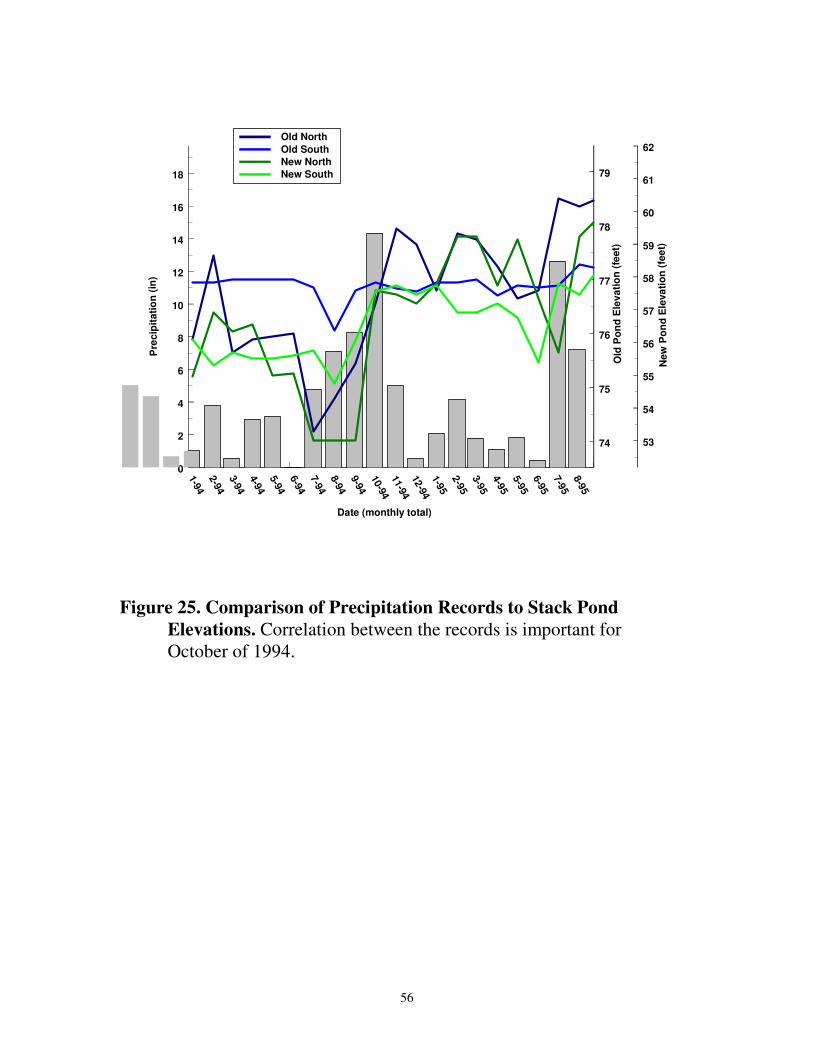
Precipitation measurements showed a high degree of correlation to stack pond
levels (figure 25) and monitor well levels (figure 26). Therefore, hydrologic controls of
these water bodies were considered to be at relative equilibrium with their environment.
Water-table levels of the stack pond were shown to be very small on a monthly scale and
found to impact ambient levels only during large precipitation events, as depicted in the
records for October of 1994. Water-table elevations in monitoring wells are seen to
recover within weeks, owing to the high conductivity of the sandy composition in the
surficial aquifer.
Annual precipitation for 1995 was 159.2 cm. with the highest monthly records in
July and August, and the lowest in the months of December and January. Precipitation
highs and lows are attributable to seasonal variations, with large annual numbers due to
the area’s latitude and proximity to the Gulf of Mexico. Annual totals are minimally
variable from year to year, and consistent in their pattern of distribution each month.
In summary, precipitation has been highly variable spatially over the area but
similar in annual totals. This will, of course, lead to localized variations of the recharge
flux into the hydrologic environment (i.e. the gypsum stack and the surficial aquifer) from
day to day, but should even out when considered on a regional scale over longer periods
of time. Large precipitation events will impact hydraulic head levels in the stack ponds
for months, while influences on the surficial aquifer are found to only last weeks.
56
1-94
2-94
3-94
4-94
5-94
6-94
7-94
8-94
9-94
10-94
11-94
12-94
1-95
2-95
3-95
4-95
5-95
6-95
7-95
8-95
Date (monthly total)
0
2
4
6
8
10
12
14
16
18
Pre
cip
itati
on
(in
)
74
75
76
77
78
79
Old
Po
nd
Ele
vati
on
(fe
et)
53
54
55
56
57
58
59
60
61
62
New
Po
nd
Ele
va
tio
n (
fee
t)
Old North
Old South
New North
New South
Figure 25. Comparison of Precipitation Records to Stack Pond
Elevations. Correlation between the records is important for
October of 1994.

57
2-223-8
3-224-9
4-235-7
5-216-4
6-187-2
7-167-30
8-138-27
9-109-24
Date
3
4
5
6
7
8
9
10H
ead
Level (f
t)
0
1
2
3
4
Pre
cip
itati
on
(in
.)
MW11
MW10
MW9
RW 13
MW3
RW 15
RW 16
MW4
RW 17
MW8
Precip.
Figure 26. Comparison of Precipitation Records to Monitor Well
Levels. Correlation between the records is important during mid-
June.

58
CHAPTER 5
GROUNDWATER FLOW MODEL
Description of the MODFLOW model
Groundwater flow at the Piney Point facility was simulated using Processing
Modflow for Windows (1994), a computer-simulation software package (hereinafter
referred to as MODFLOW) that utilizes a three-dimensional, modular finite difference
method, first developed by McDonald and Harbaugh (1988) for the U.S. Geological
Society. This modeling practice makes use of a nodal network, whereby each node
represents a hydraulic head and is modified through adherence to aquifer parameters (i.e.,
hydraulic conductivity and transmissivity ) and environmental constraints (i.e., ditches
and ponds, recharge from precipitation and evaporation ). These simulations may be run
under transient or steady-state conditions; however, only steady-state solutions are
considered here.
Mathematical Theory
Modflow simulates groundwater flow under the assumption of constant fluid
density, and generates head values for each node within its environment by solving the
following partial differential equation (groundwater flow equation) for the hydraulic head
h as a function of space (x,y,z) and time t (cf. Anderson and Woessner, 1992):
∂
∂
∂
∂
∂
∂
∂
∂
∂
∂
∂
∂
∂
∂xK
x
h yK
y
h zK
z
hS
h
tRx y z s( ) ( ) ( )+ + = −
(5.1)
59
where Kx, Ky, and Kz are hydraulic conductivity values in the x, y, and z coordinate
directions, Ss is the specific storage of the geologic unit, h is the hydraulic head, and R is
a generalized sink / source term of external nature to the system (Anderson and
Woessner, 1992).
Eq. (5.1) is used in its steady-state form by setting the dh/dt-term on the right side
to 0. The resulting steady-state groundwater flow equation changes then to the Poisson
equation which is then integrated by a finite-difference method whereby discrete head
values at each node, by using information from neighboring nodes, are iterated through
the equation until the head change between two consecutive iterations is less than a
chosen value. The numerical procedure used for the iteration process was the
Preconditioned Conjugate Gradient method.
Design of the Flow Model
The Conceptual Model
Primary consideration for the design of the conceptual model was to isolate the
stack-surficial aquifer boundary in the environment, so that a determination of the
hydrologic flux between these two units could be made from the simulated hydraulic
conditions.
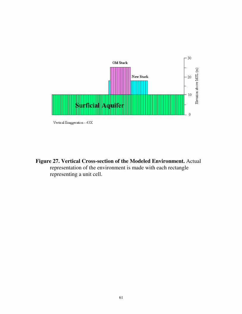
The model is comprised of two layers that represent the two aquifer units being
studied: The stack and the surficial aquifer (figure 27). The overlying stack layer consists
of two regions of 8 and 15m thicknesses, representing new and old stack accumulations,
60
respectively (figure 28), while the surficial aquifer layer is constructed as a flat-lying bed
of a constant 10 m thickness. Regions of the top layer not representing a gypsum unit are
designed to be insignificant through construction as a very thin unit (1 mm) with high
hydraulic conductivity; thus, any water contained within each unit is drained immediately
into the underlying layer and is of no consequence to any other head values.
Topography of the land surface will vary at the site, but it will have no influence
upon the hydrologic head because this value in an unconfined unit will be impacted more
by elevation of the water table. Thus, the effect of stack control on head levels in the
surficial aquifer are just as easily modeled impacting a topographically flat geologic unit
as a varied one.
Grid geometry
The simulation of the stack environment encompasses an area of 1183.36 hectares
and is organized into 6400 cells on an 80 x 80 unit grid (figure 28) . Each of the unit cells
is in a square configuration with dimensions of 43 m x 43 m, and models an actual land
surface of 1849 m2. Although the gypsum stack represents only 6.1% of the total grid, a
large modeling area was intended so that boundary conditions of the modeled
environment would not have any major effect on head values in the stack region.
61
Figure 27. Vertical Cross-section of the Modeled Environment. Actual
representation of the environment is made with each rectangle
representing a unit cell.

62
Figure 28. Specification of Layer 1 Regions. Pink cells are representative
of values in the old stack, blue cells for values in the new stack, and
green cells for the designation of insignificance in the top layer.

63
Hydrologic Parameters
Values for the hydraulic conductivities in both layers are adjusted so that the
horizontal component is calculated from the horizontal conductivity and thickness values
specified, while the vertical component is modeled in the model over the leakance values
between the stack and the surficial aquifer. The leakance value for the stack is varied in
the range of 1.0 x 10⁻²
- 1.0 x 10⁻³
day -1
, while the value at the bottom of the surficial
aquifer is specified five orders of magnitude lower, owing to the presence of the
confining Bone Valley formation. Horizontal conductivity in both units were defined
from the results of the aquifer pump tests; essentially, these estimations include the
transmissivity found for well 3-1 (0.443 m2/day) and the average of the conductivities
measured at the north and south monitoring wells (1.3 x10⁻⁶
m/s & 3.9 x10 -6
m/s).
Regions of horizontal conductivity are specified in the surficial aquifer (figure 29)
as three different sections: a sub-stack area (7.0 x 10⁻⁷
m/s), a northwest high conductivity
zone (3.9 x10 -6
m/s), and a generalized hydraulic conductivity for the remainder of the
modeled cells (1.3 x10⁻⁶
m/s). This modification was made to allow for a good match of
the modeled to the observed contoured head data.
Boundary Conditions
Constant head cells are specified in the top layer with initial head measurements of 18 m
and 25 m for the new and old stack regions, respectively (figure 27). The implication of
the constant head acting as a consistent source of water from stack ponds is intended, as
the ponds are kept at relatively constant levels from precipitation recharge.

64
Figure 29. Zones of Hydraulic Conductivity in the Surficial Aquifer.
Consecutively darker colors signify a relatively faster conductivity;
dark blue denotes a conductivity of 4.0x10⁻⁵
m/s, light blue a
conductivity of 1.3x10 -5
, and light green a conductivity of 7.0x10⁻⁶
.

65
Constant head cells are also specified at the east and west grid boundaries in
order to simulate regional groundwater flow driven by a constant gradient between these
boundaries. The angle and the slope of the regional head trend (determined from
topographical regression in chapter 4) is generated through an offset of northward
decreasing initial head values of the constant head cells. Initial head values for variable
cells of the surficial aquifer are set to 5 m.
Sources and sinks
Sources of water in the system were generated from the constant head designation
discussed above, while sinks for the system were modeled through use of the drain
package in the MODFLOW program.
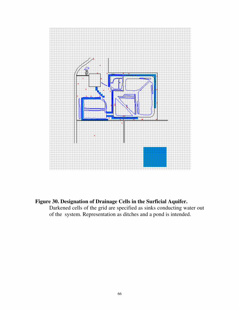
Drainage cells have been included in the top layer to simulate evaporation from
stack flanks, and in the bottom layer to model the influence of engineered ditches around
the perimeter of the stack as, well as an influential pond south of the stack (figure 30).
The insertion of drainage cells involves a specification of the drain conductance and the
elevation of the drain bottom. Drains in the top layer are specified with an elevation of 10
m and a conductance of 43 m2/day. The latter has been determined as the product of the
area, the hydraulic conductivity of the ditch fill, and the assumed thickness of the ditch
bottom.
Drains in the surficial aquifer are generally located at elevations of 3.0 & 6.0 m
with respective conductances of 43 & 21 m2/day. Drainage for the pond south of the stack
was specified at an elevation of 3.0 m, with a conductance of 43 m2/day.
66
Figure 30. Designation of Drainage Cells in the Surficial Aquifer.
Darkened cells of the grid are specified as sinks conducting water out
of the system. Representation as ditches and a pond is intended.

67
Calibration
The water table in the surficial aquifer did not vary enough to demand a complete
calibration of the model to each of the set of monitoring well head levels. Thus, a
calibration to within 10% of the average deviation for any particular head data set was
accepted as satisfactory for the steady state solution. Heterogeneities that could not be
determined or modeled within the aquifer environment were believed to be responsible
for most of the large deviations between modeled and actual head values.
Calibration of the head values in the model to their present form (figure 31) was
initiated as a large scale match to a set of contrived constant head cells which represented
values for a data set of actually measured head observations. Model parameters were then
adjusted until aberrations caused by the constant head cells disappeared and the contours
seemed adequately fit. After this was accomplished, the constant head values for
monitoring wells were taken out, and fine tuning of the parameter values was attempted.
All parameter values were kept as uniform as possible, so as to bring out inconsistencies
that would clarify local heterogeneities. Actual calibration of the model was done
conceptually in four steps:
1) balancing of stack leakance values with sub-stack conductivity to produce a head
match to well 2-0 located in the surficial aquifer,
2) adjustment of stack leakance values to generate vertical fluxes that are consistent with
the effective recharge of the gypsum stack from precipitation (minus evaporation),

68
3.0
2.02.0
3.0
4.0 5.
0
6.0
7.0
3.0
4.0
5.0
6.02.0
7.0
20.0
Figure 31. Contours of the Modeled Heads in the Surficial Aquifer.
Contours are in m intervals. Note the large influence of the cooling
pond ditches on the water table in the northeast section of the
model
3) adjustment of horizontal conductivity values in the surficial aquifer to produce head
values close to those of nearby monitoring wells,
69
4) modification of drain conductance and elevation to constrain large anomalies in head
contours.
The first two steps in the calibration involved a determination of the leakance value
trying to both match the observed hydraulic head in the surficial aquifer well 2-0 and the
estimated effective recharge of the gypsum stack as calculated from the difference
between precipitation and evaporation as measured in the region over the last few years
(see section on precipitation in the previous chapter) . Results of this calibration effort
show the strong dependency of the vertical stack-aquifer flux upon the leakance value
chosen (figure 32). With an estimated effective recharge of about 1600 m 3 /day over the
total area of both the new and the old stack, an optimal leakance value of 3 x10 -3
/day is
obtained.
In the second step, values for horizontal conductivity zones outside of the stack
region were found to be accurately quantified from the aquifer pump tests, and did not
need to be adjusted.
The final part of the calibration was made through changes in ditch elevations and
ditch conductances. Within this step was the addition of drainage cells to represent a pond
to the southeast of the stack. It was thought that impact of this pond contributed to some

70
0 1 2 3 4 5 6 7 8 9 10
Leakance
500
800
1100
1400
1700
2000
2300
2600
2900
Eff
ecti
ve R
ech
arg
e (
cu
. m
/ d
ay)
( )x day10 4 1− −
Sensitivity of Effective Stack
Recharge to Leakance
Estimated Recharge
Op
timal V
alu
e
Figure 32. Relationship of Stack Recharge to Leakance Value. Estimated
recharge values are compared to leakance values so that an optimal
leakance value can be inferred.
of the head drop from the stack in that region. The incorporation of the drainage cells
modeled partly also the effective evaporation of groundwater from the pond and from the
stack flanks, the exact value of which was not explicitly known in this study.

71
Comparison of modeled head values to observed values for September 19, 1996
(figure 20) was made to ensure a model fit (Table 5 & figure 33). The average deviation
of modeled values from well measurements was found to be 24 centimeters, which
approximated an 8.7% variance from actual values. The largest deviation of modeled
head was found to be at MW 5, which is isolated in an agricultural field south of the
research area, and could possibly be under influence of additional hydrologic factors not
considered, (i.e. irrigation pumping). Another significant deviation is exhibited at well
RW 17, which by itself is an anomaly. Contour plots of observed data (figures 19 & 20)
show that RW 17 forces a loop in the 3 m equipotential contour around the complex area.
This pattern is not quite understood, but may be the influence of a high conductivity
region or additional recharge to the groundwater in that area.
Sensitivity Analysis
Values of significance to the calibration of the model were also prime candidates
for a sensitivity analysis of the hydrologic control parameters in both the gypsum
stack and the surficial aquifer. Modeled parameters for leakance, hydraulic conductivity
and ditch specifications were modified over a range of one order of magnitude in either
direction to investigate their relative effect on the contoured modeled heads.
Table 5. Model Output Comparison to Actual Head Values. Comparison is expressed
as both an absolute depth value (in meters above MSL) and as a percentage.

72
W ell num ber 9/19/96 Value M odeled Value D ifference Percentage
M W 1 7.59 7.3 -0.29 -3.82
M W 2 4.17 4.3 0.13 3.12
M W 3 3.08 3.18 0.10 3.25
M W 4a 1.64 1.84 0.20 12.20
M W 5 1.74 2.61 0.87 50.00
M W 8 1.53 1.73 0.20 13.07
M W 9 6.39 5.24 -1.15 -18.00
M W 10 6.82 6.99 0.17 2.49
M W 11 7.26 7.24 -0.02 -0.28
RW 8 7.27 7.22 -0.05 -0.69
RW 9 5.55 5 -0.55 -9.91
RW 10 4.04 4.37 0.33 8.17
RW 11 2.73 2.72 -0.01 -0.37
RW 12 2.97 3.41 0.44 14.81
RW 13 2.91 3.54 0.63 21.65
RW 14 3.39 3.65 0.26 7.67
RW 15 2.44 2.14 -0.30 -12.30
RW 16 1.86 1.89 0.03 1.61
RW 17 3.43 2.7 -0.73 -21.28
RW 18 1.57 2.27 0.70 44.59
RW 19 2.18 2.36 0.18 8.26
RW 20 3.12 3.64 0.52 16.67
RW 21 3.20 3.23 0.03 0.94
RW 22 3.06 3.38 0.32 10.46
RW 23 2.90 3.15 0.25 8.62
RW 24 2.61 3.36 0.75 28.74
USGS 8 6.99 6.76 -0.23 -3.29
USGS 9 4.15 4.51 0.36 8.67
PZ 34 6.58 7.04 0.46 6.99
PZ 36 6.33 6.28 -0.05 -0.79
PZ 37 6.04 6.08 0.04 0.66
Stack 2 - 0 11.73 11.73 0.00 0.00
Average 0.24 8.70

73
0 1 2 3 4 5 6 7 8 9 10 11 12 13
Observed Head (m)
0
1
2
3
4
5
6
7
8
9
10
11
12
13
Mo
de
led
Hea
d (
m)
Figure 33. Modeled versus observed head values. Shown are the
listed values of table 5 with the +/- 1m error band between modeled
and observed heads
Leakance
Uniform leakance volumes from beneath the stack were the most critical value in
reference to overall head values for the entire grid. Conceptually, the leakance was
important in supplying the general volume of water available for flow into the stack and

74
the surficial aquifer. The sensitivity of the effective recharge from the stack ponds and,
owing to a lack of information, neglecting the flank water losses, ergo the flux into the
surficial aquifer to the leakance value chosen can be clearly observed from figure 32.
Thus a variation of a unit change in the leakance was found to increase head levels
beneath the stack on the meter-scale, with a modification by one order of magnitude
leaving too much of an impact on volume fluxes of water into the surficial aquifer. Thus,
the physical flux through the confining layer between the gypsum stack and the surficial
aquifer surface has the most significant impact on the modeled environment.
Conductivities
Modeled conductivity values in the surficial aquifer zones were found to
definitely be within at least one order of magnitude of their actual, measured “group”
quantity. Modification of these values by single units allowed for better model fits to
some data sets, but not to others. Since a generalized, rather homogenous hydraulic
conductivity was intended, the best fit for a generic head representation of observed
values yielded the best solution (as indicated by the differences between modeled and
observed heads of table 5) in the steady state mode. Thus, the modeled values for the
hydraulic conductivities are probably within a range of 5 units from the actual values
determined from the aquifer pump tests (cf. figure 29). It is thought that internal
heterogeneities of the hydraulic conductivity are responsible for localized head anomalies.
Ditch Specifications
Ditch elevation and conductance was determined to be of the most importance to
sinks within the hydrologic environment. Although conductance signified the degree of

75
impact each ditch had, the elevation of the ditches was a limiting factor on whether or not
any impact would be made to the flow system. The presence of ditches within the system
therefore, were a crucial part of the flow barrier surrounding the stack. Actual values of
the ditch elevations were critical to head values nearer to the stack, and although these
numbers were not directly specified from engineered specifications, slight modifications
of the elevation could be made up with additional conductance (which was also not
quantified to specifications but rather to the model fit). Regardless, ditch presence was
absolutely necessary and its parameters could not be altered very much.
As an example of the sensitivity of the model to the conductance of the ditches,
figure 34 illustrates a case whereby a conductance of 0.43 m2/day, instead of the 43
m2/day in figure 31, was used for the cooling pond ditches. With such a low conductance
the inclination of the head contours toward the cooling pond in the western part of the
model , as indicated by the actual heads (figure 20), has nearly disappeared.
Predictions for alteration of the hydrologic system are somewhat restricted to a
change in ditch presence, owing to the fact that hydraulic conductivities and water
recharge from the stack will most likely not change. Filling in of ditches will allow a

76
3.0
2.0
4.0
5.0
6.0
7.0
3.0
4.0
5.0
6.0
2.0
7.0
20.0
Figure 34. Sensitivity of the Modeled Heads in the Surficial Aquifer to
the conductance of the cooling pond ditches. In comparison with
figure 30 where a conductance of 43 m2/day was used, this one here
is only 0.43 m2/day.
larger transfer of groundwater from the stack into the surficial aquifer, and will create a
larger impact (mounding effect) of the stack on the surficial aquifer. Quantification of this

77
influence will be dependent upon how much of the ditch is actually filled in. Greatest
influence of such a change would be made to the west and southwest perimeters, as the
head gradients in those ditches support the largest volume of water conducted out of the
system. As a recommendation for future studies of the problem, ditch elevations should
be monitored more precisely than has been undertaken during the course of this
investigation.
Water Budget Analysis
A volumetric flux analysis of the surficial aquifer (figure 35) shows the actual
impact of the stack on the surficial aquifer. Values for fluxes of the hydraulic system as
obtained from the MODFLOW program and from measured hydrological input
parameters made possible such an analysis of the total water budget of the aquifer system
(stack plus surficial aquifer).
The volumetric calculation of the budgets were made in terms of m3/day and
followed the generalized form of the continuity equation:
Input - Output = Change in Storage
Although there is a short term (weekly and seasonal) change in storage which is indicated
by water level changes in the stack ponds, it can be assumed that there is no

78
PrecipitationPond Evaporation
Flank Evaporation
Dewatering Pipes
????
????
Stack Infiltration
Regional Outflow
Ditch Drainage
Regional Inflow
46 3m day/62 3
m day/
1575 3m day/
15913
m day/
1591 3m day/
31823
m day/
Figure 35. Water Budget Analysis. Input and output of volumetric fluxes
to the gypsum stack and the surficial aquifer are represented as
arrows.

79
change in storage over longer periods that are of the order of the residence times of water
in the gypsum stack and the surficial aquifer (i.e. several seasons and years). Thus, input
will equal output, as required in the steady-state model.
The volumetric input flux of the stack is described completely upon the
precipitation, with large contributors of output flux being pond evaporation and stack
leakance to the surficial aquifer. Pond evaporation was calculated as 50 % of the input
flux, with the leakance taken from a water budget file in MODFLOW. Actual fluxes were
only modeled after pathways that were known, so that smaller pathways of output fluxes
such as flank evaporation, dewatering pipes, and sprayers on top of the stack were not
considered. Upon determination of larger contributions of these smaller fluxes to the total
net output, a smaller vertical flux to the surficial aquifer could be calculated in the future.
The value determined here (figure 35) is, therefore, most likely overestimated by an
unspecified amount and would thus represent a worst-case scenario for the infiltration of
possibly toxic leachates from the phosphogypsum tailings into the surficial aquifer.
With these reservations, the inputs for the surficial aquifer unit include an
(overestimated) leakance from the gypsum stack and transport of regional flow from the
southeast. Outputs include the ditch system, as well as regional losses of groundwater to
the northwest. Most important of to this flux analysis is the comparison of regional flow
input and output to the relative inputs and outputs of the stack and ditches. For the most
part, volumes of water transferred from the stack are taken up entirely by the ditch
system. Any volume of water not taken up by the ditches is added into the regional flow
and seen as a hydrologic impact from primarily the stack; i.e. the mounding effect. This
conceptualization of the flux budget is important for the understanding of the hydraulic

80
control of water in the system. A relatively complete consumption of water to the ditches
indicates that engineering of the hydraulic balances used to minimize impact on the
groundwater are fairly adequate and even if toxic leachate from the gypsum’s stack
infiltrates into the surficial aquifer, it will, to a large extent, be intercepted by the ditch
drainage system. Figure 34 illustrates that only about 16 m3/day of water is bypassing
the ditch structure and being swept with the regional flow. Although such an amount of
non-captured diluted leachate may seem large at first glance, the value must be taken to
be relative to total fluxes in the system. When compared to the input of the surficial
aquifer, it is ~38% of that value, however, in comparison to the stack leakance, this
value is ~1% of the infiltrating flux. Thus, the addition of water to the system is quite
small in comparison to the amount of water that could be impacting the aquifer were
there no ditches. However, the quantity of flux to the system is quite large when
considering the regional flow and must be taken as somewhat of a considerable impact to
the groundwater environment in the vicinity of the phosphogypsum stack.
81
CHAPTER 6
CONCLUSIONS
This study investigates one particular phosphogypsum stack and its environment,
in an attempt to characterize flow processes that would be typical for many of the other
stacks in west central Florida. In an effort to assess flow and transport in a specific
phosphogypsum stack and the possible interaction of the low pH stack solutions with
groundwater in the adjacent surficial aquifer, a comprehensive investigation that included
hydrological testing and flow modeling has been carried out.
Several wells were drilled into the stack and the adjacent aquifer and various
experimental aquifer tests were performed and head measurements over a period of about
18 months taken. The aquifers tests include pressure transducer tests, pump and recovery
tests such as the Cooper-Jacob straight-line method, the Kirkham auger hole test and the
Bouwer Rice test for partially screened and partially penetrating wells, and in situ
flowmeter tests which allow the determination of the vertical stratification of the
hydraulic conductivity.
The pressure transducer tests provide evidence for small vertical gradients that are
reflecting the mounding effect of the stack, accentuated by the presence of a standing
water pond on its top. Although the pump tests result in only average values of the
transmissivity and storativity of the phosphogypsum stack, together with the vertical head
gradients, it hints of some vertical recharge into the gypsum formation and, because of a
significant head gradient between the gypsum stack and the underlying surficial aquifer,
possibly of vertical leakage of gypsum water into the surficial aquifer.

82
The Bouwer Rice pump tests resulted in an anomalously low hydraulic
conductivity beneath the gypsum stack but indicated a high conductivity zone in the
northwest section of the model area. The results of the flowmeter tests for the hydraulic
conductivity support the notion that flow may be partly only along horizontal bedding
planes that were formed during the `sedimentation' process of the phosphogypsum slurry.
The hydrological data was used in a steady-state numerical mounding model using
the MODFLOW model to simulate the hydraulic effect of the stack on the regional flow
and to quantify flux rates from the phosphogypsum stack into the surficial aquifer. The
model was calibrated to within 10% of the average deviation for any particular observed
head data set by adjusting various hydrological input parameters, namely the horizontal
conductivity values in the surficial aquifer; the stack leakance values, and the drain
conductances and elevation of the dewatering ditches.
The sensitivity analysis of the hydrologic control parameters in both the
gypsum stack and the surficial aquifer illustrates that the model is the most sensitive to
the leakance rate and the ditch specifications. By adjusting the vertical stack leakance
values in the model, such as to generate vertical fluxes that are consistent with the
effective recharge of the gypsum stack from precipitation, an optimal value of 3 x10 -4
day -1
was found for the leakance.
The volumetric flux analysis of the surficial aquifer shows the actual impact of
the stack on the surficial aquifer and illustrates furthermore the effectiveness of the ditch
drains in intercepting possible toxic leachate that may have infiltrated from the gypsum
stack into the surficial aquifer. In fact, only a small amount of ~1% of the infiltrating flux
of gypsum stack water is not captured by the ditches and is carried further horizontally

83
through the surficial aquifer. However, because of the neglect of the, heretofore,
unknown estimates of stack water losses due to flank evaporation, spray losses, and
dewatering pipes, the real rate of infiltration may even be less than the value indicated by
the budget analysis presented here. Unfortunately, a more precise evaluation of the true
flux-impact of the phosphogypsum stack onto the surficial aquifer will be possible only
after a more precise quantification of these stack water losses will have become
available.
REFERENCES
Amoozegar, A., and Warrick, A.W. (1986) Hydraulic conductivity of saturated soils:
field methods. Methods of Soil Analysis: Part 1 - Physical and Mineralogical
Methods, Agronomy Monograph no. 9, 735-770.
Anderson, M.P., and Woessner, W.W. (1992) Applied groundwater modeling: simulation
of flow and advective transport. San Diego, California: Academic Press Inc.,
381 pp.
Bear, J. (1979). Hydraulics of groundwater, Mc Graw-Hill Inc., New York.
Boast, C.W., and Kirkham, D. (1971) Auger hole Seepage theory. Soil Science Society of
America Proceedings, 35, 365-373.
Bouwer, H., and Rice, R.C. (1976) A slug test for determining hydraulic conductivity of
unconfined aquifers with completely or partially penetrating wells. Water
Resources Research, 12, 423-428.
Burnett, W.C., Hull, C.D., and Koch, M. (1995) How does phosphogypsum storage affect
groundwaters? Florida Institute of Phosphate Research, draft year-1 report of
project 94-05-042, 70 pp.

84
Chiang, W.H., and Kinzelbach, W. (1994) Processing Modflow for Windows : a
simulation system for modeling groundwater flow and pollution. Software
instructional manual, 196 pp.
Driscoll, F.G. (1986) Groundwater and Wells, Johnson Division, St. Paul, MN.
Gerathy and Miller, INC. (1983) Groundwater monitoring plan, Amax chemical
corporation, piney point plant. Final Report, prepared for Amax chemical
corporation (Ground Water Consultants, Tampa, Florida), 82 pp.
Gerathy & Miller, INC. (1986). Revised groundwater monitoring plan at the AMAX
Phosphate Inc. complex, Technical Report, Gerathy & Miller Inc., Tampa, FL.
Johnston, R.H., Healy, H.G., and Hayes, L.R. (1981) Potentiometric surfaces of the
tertiary limestone aquifer system, southeastern United States: May, 1980. U.S.
Geological Survey, open file report 81-486, 1 pp.
Johnston, R.H., Krause, R.E., Meyer, R.W., Ryder, P.D., Tibbals, C.H., and Hunn, J.D.
(1980) Estimated potentiometric surface for the tertiary limestone aquifer system,
southeastern United States, prior to development. U.S. Geological Survey, open
file report 80-406, 1 pp.
Lewelling, B.R., and Wylie, R.W. (1993) Hydrology and water quality of unmined and
reclaimed basins in phosphate mining areas, west-central Florida. U.S. Geological
Survey, water resources investigations report 93-4002, 93 pp.
May, A., and Sweeney, J.W. (1983) Evaluation of radium and toxic element leaching
characteristics of Florida phosphogypsum stockpiles. Bureau of Mines, report of
investigations 8776, Tuscaloosa AL, 18 pp.
May, A., and Sweeney, J.W. (1984) Assessment of environmental impacts associated
with phosphogypsum in Florida. The Chemistry and Technology of Gypsum,
ASTM Publication 861, 116-139.
Mcdonald, M.C., and Harbaugh, A.W. (1988) MODFLOW: a modular three-dimensional
finite difference ground-water flow model. U.S. Geological Survey, open file

85
report 83-875, 528 pp.
Miller, R.L. and H. Sutcliffe, Jr., (1982) Water-quality and hydrogeological data
for three phosphate industry waste-disposal sites in Central Florida,
U.S. Geological Survey, Water Resources Investigations Report 81-84,
Tallahassee, FL..
Miller, R.L., and Sutcliffe Jr., H. (1984) Effects of three phosphate industrial sites on
ground-water in central Florida, 1979 to 1980. U.S. Geological survey, water
resources investigations report 83-4256, 184 pp.
Molz, F.J., G.K. Boman, S.C. Young and W.R. Waltrop (1994).Borehole flowmeters:
field applications and data analysis, J. Hydrology, 163, 347—371.
Oaks Geotechnical Inc. (1980) Geotechnical investigation of the gypsum
stack complex of AMAX Phosphate Inc., Report, Oaks Geotechnical Inc.
Youngs, E.G. (1968) Shape factors for kirkham’s piezometer method for determining the
hydraulic conductivity of soil in situ for soils overlying an impermeable floor or
infinitely permeable stratum. Soil Science, 106, 235-237.

86
Appendix I: Cooper Jacob Straight-line Analyses
101 1022 3 4 5 6 7 8 9 2 3 4 5 6 7 8 9 2
Time (min)
5.0
4.8
4.6
4.4
4.2
4.0
3.8
Hyd
rau
lic H
ea
d (
m)
Well 1-1

87
10-1.0 100.0 101.0 102.0
Time (min)
11
10
9
8
7
6
5H
yd
rau
lic
Hea
d (
m)
Well 1-2

88
10-1.0 100.0 101.0 102.0
Time (min)
3.400
3.125
2.850
2.575
2.300H
yd
rau
lic
Hea
d (
m)
Well 1-3

89
100 101 102 103 6 3 8 5
Time (min)
2.7000
2.5625
2.4250
2.2875
2.1500H
yd
rau
lic
He
ad
(m
)
Well 1-4
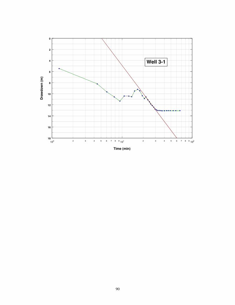
90
100 101 1022 3 4 5 6 7 8 9 2 3 4 5 6 7 8 9
Time (min)
18
16
14
12
10
8
6
4
2
0
Dra
wd
ow
n (
m)
Well 3-1

91
100 101 1029 2 3 4 5 6 7 8 9 2 3 4 5 6 7 8 9
Time (min)
4.55
4.35
4.15
3.95
3.75D
raw
do
wn
(m
)
Well 3-2

92
100 101 1029 2 3 4 5 6 7 8 9 2 3 4 5 6 7 8 9
Time (min)
3.5000
3.3875
3.2750
3.1625
3.0500D
raw
do
wn
(m
)
Well 3-3
Appendix II : Pressure Transducer Tests

93
0 2 4 6 8 10 12 14 16 18 20 22 24
Pressure (PSI)
22
18
14
10
6
2
Depth
belo
w W
ate
r T
able
(m
)
Cased Section
Screened Section
Well 1-1
94
0 2 4 6 8 10 12 14 16 18
Pressure (PSI)
17
15
13
11
9
7
5
3
1
Dep
th b
elo
w W
ate
r T
able
(m
)Well 1-2
Screened Section
Cased Section

95
0 1 2 3 4 5 6 7 8 9 10
Pressure (PSI)
10
9
8
7
6
5
4
3
2
Depth
belo
w W
ate
r T
able
(m
)
Cased Section
Screened Section
Well 1-4

96
0 2 4 6 8 10 12 14 16 18
Pressure (PSI)
19.0
17.5
16.0
14.5
13.0
11.5
10.0
8.5
7.0
5.5
4.0
De
pth
belo
w W
ell
Ris
er
(m)
Screened Section
Cased Section
Well 2-1
97
0 2 4 6 8 10 12 14 16
Pressure (PSI)
16
14
12
10
8
6
4D
ep
th b
elo
w W
ate
r T
able
(m
)
Screened Section
Well 2-2
Screened Section

98
-1 1 3 5 7 9 11 13
Pressure (PSI)
12
10
8
6
4
2D
epth
belo
w W
ate
r T
able
(m
)
Well 3-3
Cased Section
Screened Section
Appendix III : Hydraulic Head Contour Plots

99
0 250 500 750 1000 1250 1500 1750 2000 2250 2500 2750
East - West (m)
0
250
500
750
1000
1250
1500
1750
2000
2250
No
rth
- S
ou
th (
m)
5-26-96
100
0 250 500 750 1000 1250 1500 1750 2000 2250 2500 2750
East - West (m)
0
250
500
750
1000
1250
1500
1750
2000
2250N
ort
h -
So
uth
(m
)
9-19-96

101
Appendix IV : Bouwer Rice Conductivity Tests
0 600 1200 1800 2400 3000 3600 4200 4800 5400 6000
Time (sec)
0.100
1.000
10.000
Dra
wd
ow
n (
m)
Well # : MW-1
102
0 800 1600 2400 3200 4000 4800 5600 6400 7200 8000
Time (sec)
0.100
1.000
10.000D
raw
do
wn
(m
)
Well # : MW-8

103
0 400 800 1200 1600 2000 2400 2800 3200 3600 4000
Time (sec)
0.100
1.000
10.000
Dra
wd
ow
n (
m)
Well # : MW-9

104
0 240 480 720 960 1200 1440 1680 1920 2160 2400
Time (sec)
0.010
0.100
1.000
10.000
Dra
wd
ow
n (
m)
Well # : MW-18

105
0 250 500 750 1000 1250 1500 1750 2000 2250 2500
Time (sec)
0.010
0.100
1.000
10.000
Dra
wd
ow
n (
m)
Well # : MW 21
106
-0 200 400 600 800 1000 1200 1400 1600 1800 2000
Time (sec)
0.100
1.000
10.000
Dra
wd
ow
n (
m)
Well # : MW 22
107
0 500 1000 1500 2000 2500
Time (sec)
0.100
1.000
10.000
Dra
wd
ow
n (
m)
Well # : MW 24
108
0 2500 5000 7500 10000 12500 15000 17500 20000 22500 25000
Time (sec)
1.000
10.000
Dra
wd
ow
n (
m)
Well # : 2-0