modeling the subsurface structure of sunspots
TRANSCRIPT
Solar Phys (2010) 267: 1–62DOI 10.1007/s11207-010-9630-4
Modeling the Subsurface Structure of Sunspots
H. Moradi · C. Baldner · A.C. Birch · D.C. Braun · R.H. Cameron · T.L. Duvall Jr. ·L. Gizon · D. Haber · S.M. Hanasoge · B.W. Hindman · J. Jackiewicz · E. Khomenko ·R. Komm · P. Rajaguru · M. Rempel · M. Roth · R. Schlichenmaier · H. Schunker ·H.C. Spruit · K.G. Strassmeier · M.J. Thompson · S. Zharkov
Received: 27 December 2009 / Accepted: 23 August 2010 / Published online: 19 October 2010© Springer Science+Business Media B.V. 2010
Invited Review.
H. Moradi · R.H. Cameron · L. Gizon (�) · S.M. Hanasoge · H. SchunkerMax-Planck-Institut für Sonnensystemforschung, 37191 Katlenburg-Lindau, Germanye-mail: [email protected]
C. BaldnerDepartment of Astronomy, Yale University, P.O. Box 208101, New Haven, CT 06520, USA
A.C. Birch · D.C. BraunA Division of NorthWest Research Associates, Inc., Colorado Research Associates, 3380 MitchellLane, Boulder, CO 80301-5410, USA
T.L. Duvall Jr.Laboratory for Solar Physics, NASA/Goddard Space Flight Center, Greenbelt, MD 20771, USA
D. Haber · B.W. HindmanJILA, University of Colorado, Boulder, CO 80309-440, USA
J. JackiewiczAstronomy Department, New Mexico State University, P.O. Box 30001, MSC4500, Las Cruces,NM 88003, USA
E. KhomenkoInstituto de Astrofisica de Canarias, 38205, C/Via Láctea, s/n, Tenerife, Spain
R. KommNational Solar Observatory, Tucson, AZ 85719, USA
P. RajaguruIndian Institute of Astrophysics, Bangalore, India
M. Rempel · M.J. ThompsonHAO/NCAR, P.O. Box 3000, Boulder, CO 80307, USA
M. Roth · R. SchlichenmaierKiepenheuer-Institut für Sonnenphysik, Schöneckstr. 6, 79104 Freiburg, Germany
2 H. Moradi et al.
Abstract While sunspots are easily observed at the solar surface, determining their subsur-face structure is not trivial. There are two main hypotheses for the subsurface structure ofsunspots: the monolithic model and the cluster model. Local helioseismology is the onlymeans by which we can investigate subphotospheric structure. However, as current linearinversion techniques do not yet allow helioseismology to probe the internal structure withsufficient confidence to distinguish between the monolith and cluster models, the develop-ment of physically realistic sunspot models are a priority for helioseismologists. This isbecause they are not only important indicators of the variety of physical effects that may in-fluence helioseismic inferences in active regions, but they also enable detailed assessmentsof the validity of helioseismic interpretations through numerical forward modeling. In thisarticle, we provide a critical review of the existing sunspot models and an overview of nu-merical methods employed to model wave propagation through model sunspots. We thencarry out a helioseismic analysis of the sunspot in Active Region 9787 and address the se-rious inconsistencies uncovered by Gizon et al. (2009a, 2009b). We find that this sunspot ismost probably associated with a shallow, positive wave-speed perturbation (unlike the tradi-tional two-layer model) and that travel-time measurements are consistent with a horizontaloutflow in the surrounding moat.
Contents
1 Introduction . . . . . . . . . . . . . . . . . . . . . . . . . . . . . . . . . . . . . . . 31.1 Why Sunspots Are Interesting . . . . . . . . . . . . . . . . . . . . . . . . . . . 31.2 The Need for Sunspot Models in Helioseismology . . . . . . . . . . . . . . . . 41.3 What Basic Properties Should be Included in the Models? . . . . . . . . . . . 71.4 The Premise of the Article . . . . . . . . . . . . . . . . . . . . . . . . . . . . . 7
2 Surface Observational Constraints . . . . . . . . . . . . . . . . . . . . . . . . . . . 72.1 Sunspot Formation and Evolution . . . . . . . . . . . . . . . . . . . . . . . . . 82.2 Sunspot Surface Structure . . . . . . . . . . . . . . . . . . . . . . . . . . . . . 92.3 Sunspot Thermodynamics in the Photosphere . . . . . . . . . . . . . . . . . . 122.4 The Wilson Depression . . . . . . . . . . . . . . . . . . . . . . . . . . . . . . . 13
3 The Deep Structure of Sunspots . . . . . . . . . . . . . . . . . . . . . . . . . . . . 133.1 The Anchoring Problem . . . . . . . . . . . . . . . . . . . . . . . . . . . . . . 143.2 The Issue of Flux Emergence . . . . . . . . . . . . . . . . . . . . . . . . . . . 143.3 Anchoring Where? . . . . . . . . . . . . . . . . . . . . . . . . . . . . . . . . . 15
4 Sunspot Models . . . . . . . . . . . . . . . . . . . . . . . . . . . . . . . . . . . . . 154.1 Semi-Empirical Models of the Sunspot Atmosphere . . . . . . . . . . . . . . . 154.2 Magneto-Hydrostatic (MHS) Models . . . . . . . . . . . . . . . . . . . . . . . 18
H.C. SpruitMax-Planck-Institut für Astrophysik, Karl-Schwarzschild-Str. 1, 85748 Garching, Germany
K.G. StrassmeierAstrophysikalisches Institut Potsdam, An der Sternwarte 16, 14482 Potsdam, Germany
M.J. Thompson · S. ZharkovSchool of Mathematics and Statistics, University of Sheffield, Houndsfield Road, Sheffield S3 7RH, UK
S. ZharkovMullard Space Science Laboratory, University College London, Holmbury St Mary, UK
Modeling the Subsurface Structure of Sunspots 3
4.3 Non-MHS Models . . . . . . . . . . . . . . . . . . . . . . . . . . . . . . . . . 254.4 Numerical Simulations of Radiative Magnetoconvection . . . . . . . . . . . . 27
5 Diagnostics Potential of Helioseismology . . . . . . . . . . . . . . . . . . . . . . . 296 Numerical Forward Modeling of Waves Through Model Sunspots . . . . . . . . . 30
6.1 Numerical Methods . . . . . . . . . . . . . . . . . . . . . . . . . . . . . . . . . 306.2 Background Models Stabilized Against Convective Instability . . . . . . . . . 316.3 Numerical Codes . . . . . . . . . . . . . . . . . . . . . . . . . . . . . . . . . . 316.4 Eikonal Methods . . . . . . . . . . . . . . . . . . . . . . . . . . . . . . . . . . 34
7 Update on the Analysis of AR 9787 . . . . . . . . . . . . . . . . . . . . . . . . . . 357.1 Travel-Times Comparison: Time – Distance and Helioseismic Holography . . 357.2 Frequency Dependence of One-Way Travel Times . . . . . . . . . . . . . . . . 357.3 Effects of Filtering on Travel Times . . . . . . . . . . . . . . . . . . . . . . . . 377.4 Ring-Diagram Structure Inversions . . . . . . . . . . . . . . . . . . . . . . . . 397.5 Moat Flow: Hankel Analysis . . . . . . . . . . . . . . . . . . . . . . . . . . . . 427.6 Ring-Diagram Analysis of Flows . . . . . . . . . . . . . . . . . . . . . . . . . 427.7 Acoustic Halos . . . . . . . . . . . . . . . . . . . . . . . . . . . . . . . . . . . 457.8 Comparison of Observed Cross-Covariances with Simulations . . . . . . . . . 47
8 Discussion and Perspective . . . . . . . . . . . . . . . . . . . . . . . . . . . . . . . 488.1 Sunspot Structure: A Critical Assessment of Existing Models . . . . . . . . . 488.2 The Starspot Connection . . . . . . . . . . . . . . . . . . . . . . . . . . . . . . 528.3 Conflicting Helioseismic Observations . . . . . . . . . . . . . . . . . . . . . . 528.4 Emergence of a New Paradigm in Sunspot Seismology . . . . . . . . . . . . . 54
Acknowledgements . . . . . . . . . . . . . . . . . . . . . . . . . . . . . . . . . . . . 54References . . . . . . . . . . . . . . . . . . . . . . . . . . . . . . . . . . . . . . . . . 55
1. Introduction
1.1. Why Sunspots Are Interesting
Sunspots are the surface manifestations of intense magnetic-flux concentrations that haveintersected with the solar surface. As such, they represent one of the major connections ofthe internal magnetic field of the Sun with its wider environments and are the main sites ofsolar-activity phenomena. They are at the center of many ongoing challenges in the studyof the Sun, as the structure and evolution of sunspots, individually and collectively, are stillnot fully understood.
Sunspots tend to appear at well-defined latitudes, which vary with the 11-year solar cy-cle, as summarized in the so-called butterfly diagram. Any theory of the mechanism of thesolar global dynamo has to be able to explain this collective behavior. Understanding dy-namo processes is of the utmost importance, as they are believed to play crucial roles inmany astrophysical phenomena, and sunspots are the best-known candidates to provide usimportant clues on how they operate.
While the sunspots are easily observed at the surface, determining their subsurface struc-ture is not at all trivial. There are two main hypotheses for the structure of the subsurfacemagnetic configuration of the spot: the monolithic model (e.g. Cowling, 1946, 1957, 1976)and the jellyfish/cluster/spaghetti model (e.g. Parker, 1975, 1979; Spruit, 1981; Zwaan,1981). Determining the parameters of these tubes, that is typical size, field strength etc.,will help reveal details of the operation of the solar dynamo and how magnetic field is trans-ported up through the convection zone.
4 H. Moradi et al.
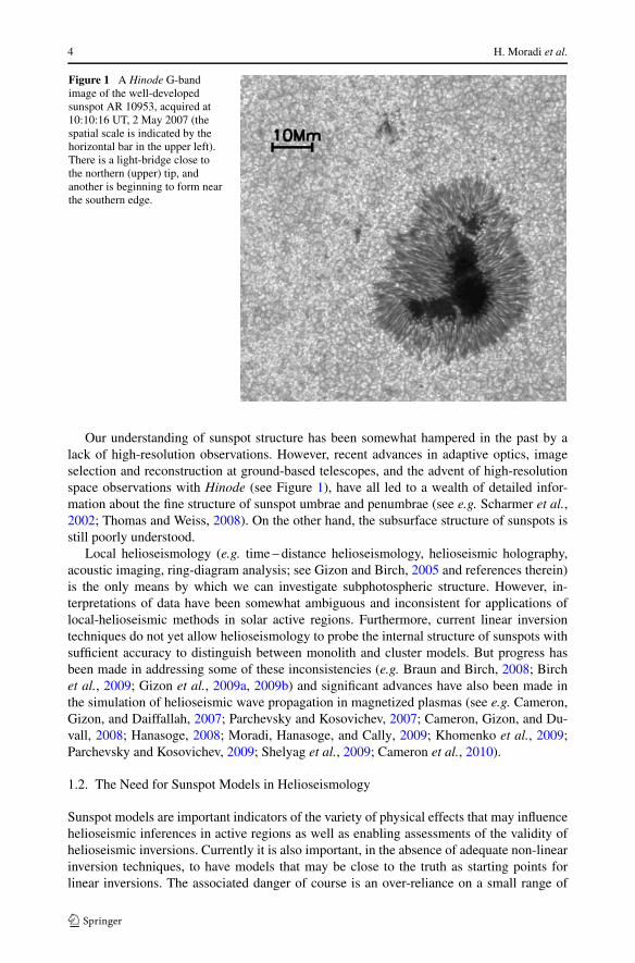
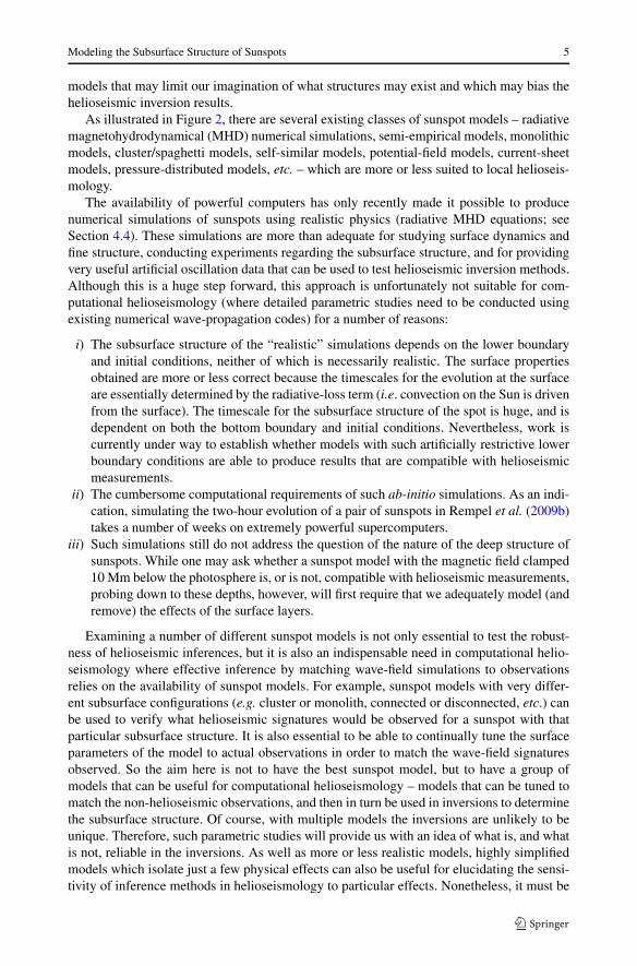
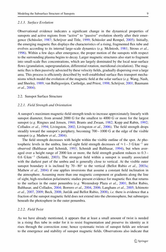
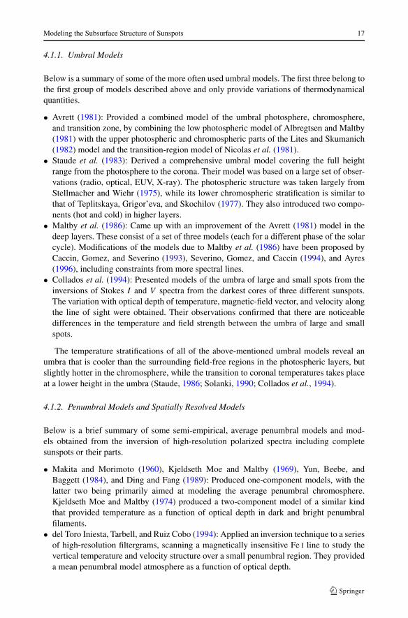
Figure 1 A Hinode G-bandimage of the well-developedsunspot AR 10953, acquired at10:10:16 UT, 2 May 2007 (thespatial scale is indicated by thehorizontal bar in the upper left).There is a light-bridge close tothe northern (upper) tip, andanother is beginning to form nearthe southern edge.
Our understanding of sunspot structure has been somewhat hampered in the past by alack of high-resolution observations. However, recent advances in adaptive optics, imageselection and reconstruction at ground-based telescopes, and the advent of high-resolutionspace observations with Hinode (see Figure 1), have all led to a wealth of detailed infor-mation about the fine structure of sunspot umbrae and penumbrae (see e.g. Scharmer et al.,2002; Thomas and Weiss, 2008). On the other hand, the subsurface structure of sunspots isstill poorly understood.
Local helioseismology (e.g. time – distance helioseismology, helioseismic holography,acoustic imaging, ring-diagram analysis; see Gizon and Birch, 2005 and references therein)is the only means by which we can investigate subphotospheric structure. However, in-terpretations of data have been somewhat ambiguous and inconsistent for applications oflocal-helioseismic methods in solar active regions. Furthermore, current linear inversiontechniques do not yet allow helioseismology to probe the internal structure of sunspots withsufficient accuracy to distinguish between monolith and cluster models. But progress hasbeen made in addressing some of these inconsistencies (e.g. Braun and Birch, 2008; Birchet al., 2009; Gizon et al., 2009a, 2009b) and significant advances have also been made inthe simulation of helioseismic wave propagation in magnetized plasmas (see e.g. Cameron,Gizon, and Daiffallah, 2007; Parchevsky and Kosovichev, 2007; Cameron, Gizon, and Du-vall, 2008; Hanasoge, 2008; Moradi, Hanasoge, and Cally, 2009; Khomenko et al., 2009;Parchevsky and Kosovichev, 2009; Shelyag et al., 2009; Cameron et al., 2010).
1.2. The Need for Sunspot Models in Helioseismology
Sunspot models are important indicators of the variety of physical effects that may influencehelioseismic inferences in active regions as well as enabling assessments of the validity ofhelioseismic inversions. Currently it is also important, in the absence of adequate non-linearinversion techniques, to have models that may be close to the truth as starting points forlinear inversions. The associated danger of course is an over-reliance on a small range of
Modeling the Subsurface Structure of Sunspots 5
models that may limit our imagination of what structures may exist and which may bias thehelioseismic inversion results.
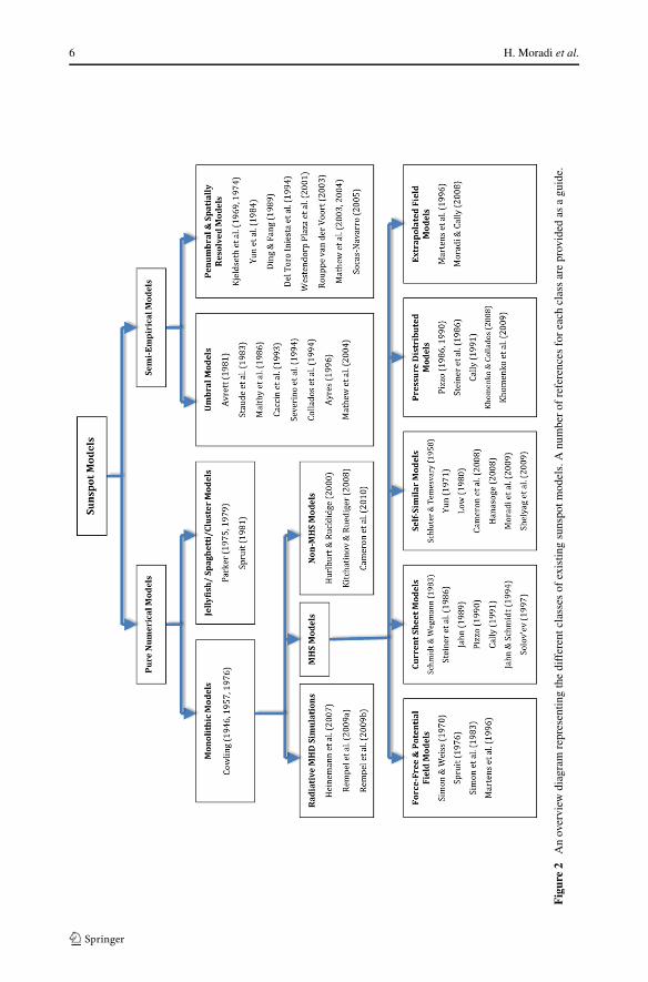
As illustrated in Figure 2, there are several existing classes of sunspot models – radiativemagnetohydrodynamical (MHD) numerical simulations, semi-empirical models, monolithicmodels, cluster/spaghetti models, self-similar models, potential-field models, current-sheetmodels, pressure-distributed models, etc. – which are more or less suited to local helioseis-mology.
The availability of powerful computers has only recently made it possible to producenumerical simulations of sunspots using realistic physics (radiative MHD equations; seeSection 4.4). These simulations are more than adequate for studying surface dynamics andfine structure, conducting experiments regarding the subsurface structure, and for providingvery useful artificial oscillation data that can be used to test helioseismic inversion methods.Although this is a huge step forward, this approach is unfortunately not suitable for com-putational helioseismology (where detailed parametric studies need to be conducted usingexisting numerical wave-propagation codes) for a number of reasons:
i) The subsurface structure of the “realistic” simulations depends on the lower boundaryand initial conditions, neither of which is necessarily realistic. The surface propertiesobtained are more or less correct because the timescales for the evolution at the surfaceare essentially determined by the radiative-loss term (i.e. convection on the Sun is drivenfrom the surface). The timescale for the subsurface structure of the spot is huge, and isdependent on both the bottom boundary and initial conditions. Nevertheless, work iscurrently under way to establish whether models with such artificially restrictive lowerboundary conditions are able to produce results that are compatible with helioseismicmeasurements.
ii) The cumbersome computational requirements of such ab-initio simulations. As an indi-cation, simulating the two-hour evolution of a pair of sunspots in Rempel et al. (2009b)takes a number of weeks on extremely powerful supercomputers.
iii) Such simulations still do not address the question of the nature of the deep structure ofsunspots. While one may ask whether a sunspot model with the magnetic field clamped10 Mm below the photosphere is, or is not, compatible with helioseismic measurements,probing down to these depths, however, will first require that we adequately model (andremove) the effects of the surface layers.
Examining a number of different sunspot models is not only essential to test the robust-ness of helioseismic inferences, but it is also an indispensable need in computational helio-seismology where effective inference by matching wave-field simulations to observationsrelies on the availability of sunspot models. For example, sunspot models with very differ-ent subsurface configurations (e.g. cluster or monolith, connected or disconnected, etc.) canbe used to verify what helioseismic signatures would be observed for a sunspot with thatparticular subsurface structure. It is also essential to be able to continually tune the surfaceparameters of the model to actual observations in order to match the wave-field signaturesobserved. So the aim here is not to have the best sunspot model, but to have a group ofmodels that can be useful for computational helioseismology – models that can be tuned tomatch the non-helioseismic observations, and then in turn be used in inversions to determinethe subsurface structure. Of course, with multiple models the inversions are unlikely to beunique. Therefore, such parametric studies will provide us with an idea of what is, and whatis not, reliable in the inversions. As well as more or less realistic models, highly simplifiedmodels which isolate just a few physical effects can also be useful for elucidating the sensi-tivity of inference methods in helioseismology to particular effects. Nonetheless, it must be
6 H. Moradi et al.
Fig
ure
2A
nov
ervi
ewdi
agra
mre
pres
entin
gth
edi
ffer
entc
lass
esof
exis
ting
suns
potm
odel
s.A
num
ber
ofre
fere
nces
for
each
clas
sar
epr
ovid
edas
agu
ide.
Modeling the Subsurface Structure of Sunspots 7
borne in mind if using such models that other physical effects may have seismic signaturesthat are qualitatively or quantitatively similar.
1.3. What Basic Properties Should be Included in the Models?
Apart from the desired characteristics mentioned above, models of the gross magnetic struc-ture of sunspots for use in computational helioseismology should ideally posses a high de-gree of flexibility and computational efficiency to allow for extensive parameter studiesusing existing numerical simulation codes. A number of other essential, observationallyderived, characteristics should also be embodied by the models. For example, an accurateprescription for the surface (photospheric) magnetic-field characteristics (of both the um-bra and penumbra, e.g. field strength, orientation, twist, return flux, etc., see Section 2.2.1and Section 2.2.2). These should comply with observations and, ideally, one should be ableto model the sunspot field on extrapolations from observed surface magnetic profiles (e.g.vector magnetograms). One should also be able to choose the profile of thermodynamic pa-rameters (pressure, density, temperature, etc., see Section 2.3 and Section 4.1) in the umbraand penumbra from either spectro-polarimetric inversions or semi-empirical models of thesolar atmosphere. Some important dynamical phenomena (e.g. the Evershed flow, moat flow,etc.; see Section 2.2.4 and Section 2.2.5) should also be taken into account, while a realisticand consistent (e.g. Section 2.4) description of the Wilson depression is also essential.
1.4. The Premise of the Article
The basic premise of this article is to satisfy two complementary goals: The first goal isto present a critical review of the existing physical models for the subsurface structure ofsunspots, in the context of local helioseismology and numerical simulations of wave fields,and magnetic field – wave interaction. As discussed above, physical sunspot models are crit-ically important to assess the validity of the helioseismic inversions. In addition, numericalsimulations of the propagation of solar waves through model sunspots are emerging as avalid and realistic technique to interpret helioseismic data. The success of this approachrelies on a very close interaction between sunspot modelers and helioseismologists.
The second goal is to extend the helioseismic analysis undertaken by Gizon et al. (2009a,2009b) of the sunspot in Active Region (AR) 9787, which was the topic of the Third HELAS(European Helio- and Asteroseismology Network) Local Helioseismology Workshop, heldin Berlin on 12 – 15 May 2009. This sunspot was observed during the period 20 – 28 January2002 by the SOHO/MDI instrument. Serious inconsistencies between the different helioseis-mic methods were uncovered, which cannot be left unanswered.
2. Surface Observational Constraints
In this section we briefly review some of the main observational characteristics of sunspotformation and evolution. The aim here is to present a very general overview of some of thepertinent issues related to sunspot observations that need to be considered when developinga realistic sunspot model. Comprehensive reviews by Solanki (2003), Thomas and Weiss(2004), Tobias and Weiss (2004), Schlichenmaier (2009), and the books by Thomas andWeiss (1992, 2008) (and references therein), have excellent extended discussions on boththe observational and theoretical aspects of sunspots and active regions.
8 H. Moradi et al.
2.1. Sunspot Formation and Evolution
2.1.1. Flux Emergence
Individual bundles of magnetic flux are believed to rise from deep in the convection zoneand break through the surface of the Sun. As they approach the surface, each flux bundle isshredded into many separate strands which, upon emergence, are quickly concentrated intosmall, intense (kG strength) magnetic flux bundles (or elements) by the vigorous convectionoccurring in the thin superadiabatic layer at the top of the convection zone. These smallflux elements then accumulate at the boundaries between granules or supergranules, andsome of them coalesce to form small pores (Keppens and Martínez Pillet, 1996; Leka andSkumanich, 1998). Some pores and flux elements in turn coalesce to form sunspots.
A number of studies have examined the buoyant rise of magnetic flux from just belowthe surface and rising into a non-magnetized atmosphere (e.g. Magara and Longcope, 2001,2003; Manchester et al., 2004; Cheung, Schüssler, and Moreno-Insertis, 2007). A number ofstudies modeling the rise of thin flux tubes through the convection zone have also shown thatthe tubes must have a significant amount of twist in order to maintain their integrity and notfragment in the face of hydrodynamic forces, and indeed observations show that magneticflux usually emerges at the surface already in a significantly twisted state (e.g. Riethmülleret al., 2008).
2.1.2. Sunspot Formation and Decay
When the flux does emerge, it is often in the form of pore structures of the order of aMm or so in size (Vrabec, 1974; Zwaan, 1978, 1992; McIntosh, 1981). Pores have con-tinuum intensities ranging from 80% down to 20% of the normal photospheric intensity,with maximum magnetic-field strengths of 1500 – 2000 G. If a growing pore reaches asufficient size (a diameter of about 3500 km, but sometimes as much as 7000 km) or asufficient total magnetic flux of order 1020 Mx (Leka and Skumanich, 1998), and if themagnetic field reaches an inclination from the vertical that is greater than about γ = 35°(Martínez Pillet, 1997), then it forms a penumbra at its periphery and becomes a full-fledged sunspot. The formation of a penumbra is a rapid event, occurring in less than20 – 30 minutes, and the characteristic sunspot magnetic-field configuration and Evershedflow are both established within this same, short time period (Leka and Skumanich, 1998;Yang et al., 2003). Furthermore, the fact that the largest pores are observed to be bigger thanthe smallest sunspots also provides evidence that the pore – sunspot transition is associatedwith hysteresis (Bray and Loughhead, 1964; Rucklidge, Schmidt, and Weiss, 1995).
The time scale for the formation of a large sunspot is between a few hours and severaldays. A sunspot can span a lifetime of months, but more typically of weeks (Solanki, 2003).However, this life expectancy is considerably shorter than the magnetic diffusion time [tD =l2/η where l is the width of the current sheet and η = 1/σ is the magnetic diffusivity] acrossa solar active region where estimates for tD range from hundreds to thousands of years (e.g.Priest and Forbes, 2000). This reduced lifetime suggests that a convective instability sets inthat enhances the decay process, via fragmentation. Another possible process is the actionof turbulent diffusion, owing to the non-linear dependence of the diffusivity on the strengthof the magnetic field (Petrovay and Moreno-Insertis, 1997). An overview of sunspot decaywas presented by Martínez Pillet (2002).
Modeling the Subsurface Structure of Sunspots 9
2.1.3. Surface Evolution
Observational evidence indicates a significant change in the dynamical properties ofsunspots and active regions from “active” to “passive” evolution shortly after their emer-gence (Schüssler, 1987; Schrijver and Title, 1999; Schüssler and Rempel, 2005). Initially,the emerging magnetic flux displays the characteristics of a rising, fragmented flux tube andevolves according to its internal large-scale dynamics (e.g. McIntosh, 1981; Strous et al.,1996). Within a few days after emergence, the proper motion of the sunspots with respectto the surrounding plasma begins to decay. Larger magnetic structures also start to fragmentinto small-scale flux concentrations, which are largely dominated by the local near-surfaceflows (granulation, supergranulation, differential rotation, meridional circulation). The mag-netic flux is then passively advected by these velocity fields, gradually dispersing over a largearea. This process is efficiently described by well-established surface flux-transport mecha-nisms which model the evolution of the magnetic field at the solar surface (e.g. Wang, Nash,and Sheeley, 1989; van Ballegooijen, Cartledge, and Priest, 1998; Schrijver, 2001; Baumannet al., 2004).
2.2. Sunspot Surface Structure
2.2.1. Field Strength and Orientation
A sunspot’s maximum magnetic-field strength tends to increase approximately linearly withsunspot diameter, from around 2000 G for the smallest to 4000 G or more for the largestsunspot (e.g. Ringnes and Jensen, 1960; Brants and Zwaan, 1982; Kopp and Rabin, 1992;Collados et al., 1994; Livingston, 2002; Livingston et al., 2006). The field strength dropssteadily toward the sunspot’s periphery, becoming 700 – 1000 G at the edge of the visiblesunspot (e.g. Mathew et al., 2004).
The field strength decreases with height within the visible outline of the spot. At pho-tospheric levels in the umbra, line-of-sight field strength decreases of ≈ 1 – 3 G km−1 areobserved (Balthasar and Schmidt, 1993; Schmidt and Balthasar, 1994), but when aver-aged over a height range of 2000 km or more, the field strength gradient reduces to 0.3 –0.6 G km−1 (Solanki, 2003). The strongest field within a sunspot is usually associatedwith the darkest part of the umbra and is generally close to vertical. At the visible outersunspot boundary it is inclined by 70 – 80◦ to the vertical (Bellot Rubio et al., 2003a;Mathew et al., 2004) if one applies inversions that assume a constant field inclination inthe atmosphere. Assuming more than one magnetic component or gradients along the lineof sight, high-resolution polarimetric studies present evidence for magnetic flux that returnsto the surface in the outer penumbra (e.g. Westendorp Plaza et al., 2001; Bellot Rubio,Balthasar, and Collados, 2004; Borrero et al., 2004, 2006; Langhans et al., 2005; Ichimotoet al., 2007, 2009; Beck, 2008; Jurcák and Bellot Rubio, 2008), i.e. there is evidence that afraction of the sunspot magnetic field does not extend into the chromosphere, but submergesbeneath the photosphere in the outer penumbra.
2.2.2. Field Twist
As we have already mentioned, it appears that at least a small amount of twist is neededin a rising flux tube in order for it to resist fragmentation and preserve its identity as itrises through the convection zone; hence systematic twists of sunspot fields are relevantto the emergence and stability of sunspot magnetic fields. Observations also indicate that
10 H. Moradi et al.
the magnetic field of regular sunspots can be twisted, with an azimuthal twist φ ≈ 10◦ – 35◦(Hagyard, West, and Cumings, 1977; Gurman and House, 1981; Lites and Skumanich, 1990;Skumanich, Lites, and Martínez Pillet, 1994; Westendorp Plaza et al., 2001).
However, the more recent observations of Mathew et al. (2003) indicate that for regu-lar isolated sunspots, the global azimuthal twist of the field does not significantly exceed20°. Moreover, Yun (1971) and Osherovich and Flaa (1983) have included the effects ofan azimuthal field twist in their (self-similar) sunspot models and find that the introductionof a moderately twisted field, compatible with observations, contributes little to the forcebalance in spots and only slightly changes the main characteristics of their sunspot models(e.g. the mixing-length parameter, effective temperature, Wilson depression, and the centralfield strength remain practically the same). This is not surprising, in view of the fact that themeasured Bψ from observations is small compared to Bz and Br over most of the sunspotregion.
2.2.3. Umbral Dots
Umbral dots, bright dot-like feature observed inside an umbra, are found in almost allsunspots and also in pores (Sobotka, 1997, 2002). They are observed to cover only 3 –10% of the umbral area but contribute 10 – 20% of the total umbral brightness (Sobotka,Bonet, and Vazquez, 1993). Their distribution is not uniform: they can occur in clusters andalignments, and no large dots are found in dark nuclei (Rimmele, 1997).
On average, umbral dots are 500 – 1000 K cooler than the photosphere outside a spot,but about 1000 K hotter than the coolest parts of the umbra itself (Kitai et al., 2007). Themagnetic field in umbral dots appears to be weaker than that in the umbral background(Sobotka, 1997). Socas-Navarro et al. (2004) found differences of several hundred gaussand deduced that the fields were more inclined to the vertical, by about 10°. Furthermore,a small upward velocity of 30 – 50 m s−1 and 200 m s−1 has been reported in umbral dotsrelative to the umbral background by Rimmele (1997) and Socas-Navarro (2002).
Schüssler and Vögler (2006) have presented realistic numerical simulations of umbralmagnetoconvection in the context of the monolithic model, by assuming an initially uniformvertical magnetic field. Their model reproduces all of the principal observed features ofumbral dots, including their dark lanes (Rimmele, 2008). Their results provide support forthe monolithic model, demonstrating that umbral dots can arise naturally as a consequenceof magnetoconvection in a space-filling vertical magnetic field. The more recent numericalsimulations of Heinemann et al. (2007) and Rempel, Schüssler, and Knölker (2009a) alsoconfirm this.
2.2.4. Evershed Flow
The Evershed flow is observed as an outward-directed (horizontal) flow observed in thephotospheric layers of penumbrae. The inverse Evershed flow is an inward-directed flow inchromospheric layers. A number of well-established observational properties of the Ever-shed flow are:
• The averaged flow velocity increases from the inner to the outer penumbra. From observedline asymmetries it is concluded that the flow is located in the deep photosphere (Maltby,1964; Schlichenmaier, Bellot Rubio, and Tritschler, 2004).
• Observed velocities of the flow typically exceed 6 km s−1 (Rouppe van der Voort, 2002;Bellot Rubio et al., 2003a) in the outer penumbra, but can also exceed 10 km s−1 inlocalized patches (e.g. Bellot Rubio, Balthasar, and Collados, 2004).
Modeling the Subsurface Structure of Sunspots 11
• The direction of the Evershed flow is close to horizontal. Azimuthal averages reveal thatthe flow angle varies from 70° (average flow points upward) in the inner penumbra tosome 100° (flow points downward) in the outer penumbra (Schlichenmaier and Schmidt,2000).
• The Evershed flow is magnetized. This is obvious from Stokes V profiles with more thantwo lobes. These additional lobes are Doppler shifted (e.g. Schlichenmaier and Collados,2002).
Two models have been proposed to explain a number of observational properties: the“siphon-flow” model as proposed by Montesinos and Thomas (1997), and the “moving-tube” model by Schlichenmaier, Jahn, and Schmidt (1998). Montesinos and Thomas (1997)elaborated on the idea of Meyer and Schmidt (1968) that the flow is driven by a gas-pressuredifference between the footpoints of a thin magnetic-flux tube in magnetohydrostatic (MHS)equilibrium. On the other hand, Schlichenmaier, Jahn, and Schmidt (1998) developed adynamical 2D model of a thin magnetic-flux tube that acts as a convective element in asuperadiabatic and magnetized penumbral atmosphere. In their model, the convective riseof the thin flux tube to the surface initiates a local pressure-gradient build up, leading to agas flow along the tube. Penumbral grains are then identified as the hot upflow locationswhere the gas reaches the (optical) surface.
Numerical simulations of radiative magnetoconvection in inclined magnetic fields (e.g.Heinemann et al., 2007; Scharmer, Nordlund, and Heinemann, 2008; Rempel, Schüssler,and Knölker, 2009a; Rempel et al., 2009b) are only beginning to reproduce the structureof the outer penumbra, with its horizontal and returning magnetic fields and fast Evershedflows along arched channels. They have already succeeded in reproducing single elongatedfilaments with lengths of up to a few Mm, which resemble in many ways what is observed asthin light bridges and penumbral filaments of the inner penumbra. In their simulations, theyfind that the progression of the filament heads toward the umbra during their formation phaseis not caused by the inward motion of a narrow flux tube, but rather due to the expansion ofthe sheet-like upflow plumes along the filament.
2.2.5. Moat Flow and Moving Magnetic Features
The moat flow is an outflow that initiates immediately after the formation of a penumbra.Moats are typically 10 to 20 Mm wide, with the outer radius of the moat appearing toscale with the size of the enclosed sunspot, being about twice the radius of the spot itself(Brickhouse and Labonte, 1988). The moat-flow velocity is about 0.5 to 1 km s−1, and canbe seen by proper motions of granules as well as by Doppler-shift measurements (Balthasaret al., 1996). The flow usually persists over the duration of the spot’s life, while the areaand magnetic flux of the sunspot decrease at a roughly constant rate. As the moat flowevolves, it pushes the magnetic flux to its periphery, leaving the moat largely free of magneticfield except for small magnetic features (known as moving magnetic features) that moveoutward across the moat at speeds of about 1 km s−1 (Sheeley, 1969, 1972; Vrabec, 1971,1974; Harvey and Harvey, 1973; Brickhouse and Labonte, 1988; Wang and Zirin, 1992;Yurchyshyn, Wang, and Goode, 2001; Sainz Dalda and Bellot Rubio, 2008a).
The moat flow is only present in the presence of a penumbra. Pores that have no penum-bra also lack the moat flow. Observations of irregular sunspots by Vargas Domínguez et al.(2007) indicate that the moat flow exists only on sunspots sides where a penumbra hasformed. On sunspot sides where the umbra and the granulation are adjacent, no moat flow isdetected. Moreover, in such irregular configurations moat flows are only observed as radialextensions of penumbral filaments, but not perpendicular to the filament.
12 H. Moradi et al.
The moat flow has also been detected through local helioseismology, using f -modetime – distance helioseismology. Using azimuthally averaged MDI data, Gizon, Duvall, andLarsen (2000) find an outflow extending well beyond the sunspot boundary (up to 30 Mm)which reaches a peak of 1 km s−1 just outside the penumbra. This flow is consistent with themoat flow. In another recent study, Gizon et al. (2009a, 2009b) used f to p4 ridge-filteredtime – distance travel times to produce linear inversion for flows around AR 9787. Theseinversions showed an azimuthally averaged horizontal outflow in the first 4 Mm beneath thesurface, reaching an amplitude of 230 m s−1 at a depth of 2.6 Mm and radial distance ofsome 5 Mm outside the outer spot boundary. The inversion results were in line with obser-vations of the moat flow in AR 9787 presented by Gizon et al. (2009a, 2009b), the strengthand extent of which was characterized by measuring the observed motion of the movingmagnetic features (MMFs) using a local correlation-tracking method. Their measurementsindicated a peak amplitude of 230 m s−1 for the moat flow, extending out to about 45 Mmfrom the spot center.
As the moat flow is unmagnetized and has velocities that are much smaller than the Ever-shed flow, the link between the two is not obvious. One possibility is that the gas pressurethat builds up beneath the penumbra could drive the moat flow (beneath the penumbra themagnetopause is largely inclined). Sainz Dalda and Bellot Rubio (2008b) detect bipolarMMFs within the penumbra, which migrate outward into and throughout the moat. This isconsistent with a scenario proposed by Schlichenmaier (2002): a magneto-convective over-shoot instability in an Evershed flow channel leads to a bipolar MMF that travels outwardalong the magnetic canopy.
2.3. Sunspot Thermodynamics in the Photosphere
There are a number of semi-empirical and observational models as reference, consistingof both one- and two-component models, for the umbra and for the penumbra (see Sec-tion 4.1 for a more detailed discussion). The basic assumption underlying almost all single-component models is that it is possible to describe all umbrae (or at least those above acertain size) by a single thermal model.
Thus, a very important question in this context is whether sunspot brightness (temper-ature) or magnetic-field strength actually varies with the size of the sunspot. Theoreticalmodels of sunspots based on MHS equilibrium and inhibition of convective heat transport(e.g. Deinzer, 1965; Yun, 1970) typically obtain lower temperatures for stronger magneticfields. However, observations by Rossbach and Schröter (1970) and Albregtsen and Maltby(1981) indicated no dependence of umbral intensity on umbral size for umbral diametersgreater than about 8′′. On the other hand, the observations of Kopp and Rabin (1992) showeda nearly linear decrease in umbral brightness with umbral radius for six sunspots. A similarresult was obtained for seven spots at visible wavelengths by Martínez Pillet and Vazquez(1993) and Collados et al. (1994). This was also confirmed in a more recent study of contin-uum images of more than 160 sunspots taken during Solar Cycle 23 by Mathew et al. (2007).Indeed, Norton and Gilman (2004) use this dependence to predict the peak field strength ofa sunspot from its brightness to an accuracy of about 100 G. Hence, even though the rel-atively homogeneous umbral nuclei cannot be described by a single universal atmosphere,these models may nonetheless be used as boundary conditions in theoretical global sunspotmodels.
Another related question is whether the umbra – photosphere brightness ratio of largesunspots varies over the solar cycle. Albregtsen and Maltby (1978, 1981) find that sunspotswere darkest at the beginning of Sunspot Cycle 20 and that spots appearing later in the cy-cle were progressively brighter (with a nearly linear dependence on the phase of the cycle),
Modeling the Subsurface Structure of Sunspots 13
up until the new Cycle 21 spots appeared, which were again darkest. Subsequent observa-tions showed that the same behavior occurred in Cycle 21 (Maltby et al., 1986). Penn andLivingston (2006) found similar behavior during Cycle 23. However, the results of Mathewet al. (2007) find no significant change in umbral brightness over Cycle 23.
2.4. The Wilson Depression
The reduced opacity in a sunspot, and the consequent depression of the τ = 1 level, arisesmainly from two effects: i) the reduced temperature in the spot atmosphere leads to a de-crease in the H− bound-free opacity, and ii) the radial force balance (including magneticpressure and curvature forces) demands a lower gas pressure within the spot, further reduc-ing the net opacity.
A purely observational determination of the Wilson depression is complicated by evo-lutionary changes in the shape of the spot. Estimates from observations range from400 – 1500 km for mature spots (Bray and Loughhead, 1964; Gokhale and Zwaan, 1972;Balthasar and Wöhl, 1983). Martínez Pillet and Vazquez (1993) assume a linear relation be-tween magnetic pressure and temperature in a spot (as indicated by observations), in whichcase the radial force balance yields a simple relationship between the net magnetic curva-ture force and the Wilson depression. They computed a Wilson depression of 400 – 800 kmin the umbra of their observed sunspot (the range being due to different assumed values ofthe curvature forces). Solanki, Walther, and Livingston (1993) and Mathew et al. (2004)used this approach to determine the variation of the Wilson depression with radius acrossa sunspot. They found values of some 100 km in the penumbra and some 400 km in theumbra, with a fairly sharp transition at the umbra – penumbra boundary. In a more recentstudy, Watson et al. (2009) compared observations of sunspot longitude distribution andMonte Carlo simulations of sunspot appearance using different models for spot growth rate,growth time and depth of Wilson depression, deducing a mean depth for the umbral τ = 1layer of 500 – 1500 km.
3. The Deep Structure of Sunspots
Though the small-scale structure seen at the surface of a sunspot is not exactly in equilib-rium, the spot itself survives on much longer time scales than would be expected if it werea superficial structure. It lives much longer than the time scale on which it would evolve ifit were not in a stable equilibrium, which is the time for the Alfvén speed to cross the spot(on the order of an hour).
The magnetic field of a spot cannot be just a surface phenomenon, however, sincemagnetic-field lines have no ends. The extension of the spot’s field lines above the solarsurface can be observed in the chromosphere and corona, but they must continue belowthe surface as well. In contrast with a scalar field such as pressure, the magnetic field of asunspot cannot be kept in equilibrium simply by pressure balance at the surface: the tensionin the magnetic-field lines continuing below the surface exerts forces as well. The questionof spot equilibrium thus involves deeper layers, down to wherever the field lines continue.This is the well-known “anchoring” problem of sunspots (Parker, 1979): at which depth, andby which agent is the sunspot flux bundle kept together?
14 H. Moradi et al.
3.1. The Anchoring Problem
As an answer to this problem, Parker (1979) postulates the existence of a horizontal flow atsome depth below the surface, converging on and flowing through the magnetic-flux bundleof the spot. The drag force of this flow on the field would prevent the bundle from frag-menting. There are some obstacles to this idea. A horizontal flow is observed around spots(the moat flow), but it is of the opposite sign to the proposed inflow. There is no theory forthe cause of the proposed flow of Parker (1979). In fact, the “heat-flux blocking” by thesunspot would cause a flow of opposite sign, and this is actually observed in the form ofthe moat flow. It is also questionable if the proposed flow would actually be sufficient tokeep the flux bundle together, in view of the (interchange) instabilities to be expected in thispicture (Schüssler, 1984). What has kept Parker’s proposal alive, however, is the helioseis-mic inference (Duvall et al., 1996) of a huge downflow of 2 km s−1 of the sign proposedby Parker. It is a puzzling observation, which, if confirmed, would require new theoreticalideas. However, more recent helioseismic inferences derived from inversions of subsurfaceflows around the sunspot in AR 9787 (see Section 7.6.2) do not confirm the existence of thisdownflow.
A second proposal (already implicit in Cowling, 1953, and developed by Babcock, 1963;Leighton, 1969; Spruit and Roberts, 1983) is that the flux bundle of a spot actually continuesall of the way to the base of the convection zone, to the layer of toroidal field from which theactive region erupted. At this depth, a field strength of ≈ 80 kG is inferred from flux-tubeemerging calculations (see e.g. D’Silva and Choudhuri, 1993; Caligari, Moreno-Insertis, andSchüssler, 1995). The Alfvén travel time for a change at the base to propagate to the surface(more accurately: the propagation time of a transverse tube wave) is then about five days.This is the time scale on which the spot would change if there were nothing to maintainconditions at the base. The idea is thus that a spot, while in equilibrium at the surface, wouldactually be a transient structure in the layers from which its magnetic field originates. Thisproposal agrees roughly with the lifetime of most small spots. It is too short, however, toexplain the anchoring of stable, long-lived spots.
3.2. The Issue of Flux Emergence
The anchoring problem of long-lived spots is thus still somewhat open. Quite clear, how-ever, is the picture of flux emergence: the process by which a loop of flux rises froma horizontal layer of magnetic flux at the base of the convection zone to form an ac-tive region, as discussed briefly in Section 2.1.1. Simplified 1D calculations in the “thintube” approximation (D’Silva and Choudhuri, 1993; Fan, Fisher, and McClymont, 1994;Caligari, Moreno-Insertis, and Schüssler, 1995) point to a field strength of about 105 G atthe base of the convection zone. At this strength, agreement is reached with three inde-pendent key properties of active regions: i) the time scale of emergence (a few days), ii) theheliographic-latitude range of emergence, and iii) the tilt of active-region axes (e.g. Caligari,Schüssler, and Moreno-Insertis, 1998, and references therein). This is also the field strengthat which the horizontal field is first expected to become unstable to the development of bendsin the field lines, creating loops rising to the surface (Schüssler et al., 1994).
However, the picture presented by rising flux-tube simulations is somewhat incomplete,since the last stages of the flux-emergence process in the near-photospheric layers are typi-cally excluded. It has been pointed out by Schüssler and Rempel (2005) that the typical sizeof active regions corresponds to a wavenumber of m = 10 to 60, while buoyant flux tubestypically prefer m = 1 or 2 instabilities. From this mismatch in scales one would expect an
Modeling the Subsurface Structure of Sunspots 15
unrealistic drift of sunspots apart from each other much further than actually observed dueto magnetic tension forces. Possible solutions could include a “dynamical disconnection” assuggested by Schüssler and Rempel (2005) or a flux-emergence process that prefers largerwave numbers from the beginning. Observational evidence for this process has recently beenprovided by Svanda, Klvana, and Sobotka (2009).
Overall, the convergence of these lines of evidence supports the basic correctness of theflux-emergence picture of active-region formation that has long been intuitively evident fromobservations (Cowling, 1953). It has the important implication that the energy density of themagnetic field at its source is more than two orders of magnitude larger than energy densityin convective flows; at such a strength the field is nearly unaffected by convective flows.The same is the case at the surface of a sunspot. This is incompatible with the cornerstoneof traditional mean-field dynamo models based on the effect of convective turbulence act-ing on magnetic fields. The picture sketched above and the mean-field convective dynamomodel thus cannot both be correct. This fact is remarkably politely ignored in discussionson theories of the solar cycle.
3.3. Anchoring Where?
Some details of the evolution of an active region give additional clues about the anchoring ofsunspots. After their formation, long-lived spots wander about a bit in longitude and latitude(e.g. like AR 9787, Gizon et al., 2009a, 2009b), settling to their final position over the courseof a few days (e.g. Mazzucconi, Coveri, and Godoli, 1990). This is similar to the inferredAlfvén travel time from the base of the convection zone and the surface. The observedsettling process thus agrees with the notion of anchoring in deep layers. The “settling timescale”, the Alfvén travel time from the anchor to the surface, agrees with the field strength atthe base of the convection zone inferred from the other properties of the emergence processmentioned above.
While anchoring at the base of the convection zone thus agrees with a range of obser-vational indications, this does not in itself prove that other locations within the convectionzone are excluded. Such locations are, however, somewhat unlikely. Apart from the bound-ary with the stably stratified interior, it is hard to find a plausible location for anchoring amagnetic field in a convecting stellar envelope, which is itself unstable to fluid displace-ments. The anchor of a long-lived spot needs to act over a time longer than the convectiveturnover time of the envelope as a whole (which would be on the order of a month, in theclassical mixing length view).
4. Sunspot Models
4.1. Semi-Empirical Models of the Sunspot Atmosphere
Semi-empirical models of umbral or penumbral atmospheres give the variation of thermo-dynamic variables and magnetic-field vector with optical depth based on empirical data andtheoretical considerations of mechanical equilibrium and radiative transfer. Semi-empiricalmodels can be divided into two groups, based on the observational material and methodsused for their derivation.
One group consists of spatially unresolved, one-dimensional models based on multi-wavelength observations of the continuum, weak and strong spectral lines. The general pro-cedure in constructing a model atmosphere usually involves first determining a temperature –optical depth relation, as a best fit to the empirical data, and then determining the gas and
16 H. Moradi et al.
electron pressures by integrating the equation of hydrostatic equilibrium. In general, a num-ber of assumptions/generalizations are made when calculating this type of semi-empiricalmodels:
i) For the lower photospheric layers, measurements of the center-to-limb variation of con-tinuum intensity at several spectral intervals and the profiles of the weak spectral lines(or the wings of strong lines) are used together with the LTE assumption. For the highchromospheric layers, strong spectral lines are used such as Ca II H and K and IR lines,Hα, Na I D, etc. and the analysis is carried out in NLTE.
ii) Hydrostatic equilibrium is assumed. The question of the magnetic-field distribution isnot addressed.
Most models consist of a single component, meant to represent a horizontal average overthe umbra or penumbra, while a number of models consist of two components, designedto treat bright and dark regions separately in observations that do not fully resolve themspatially.
Another group of models uses a relatively new strategy based on the inversion of thepolarized light radiative-transfer equation (e.g. Ruiz Cobo and del Toro Iniesta, 1992). Theinput data for these models are spectro-polarimetric or spectral observations (typically ofhigh resolution). Formal mathematical methods are used to find the best fit to the spectral-line profiles and only a few spectral lines are required to produce a model atmosphere. Thismethod provides sunspots models (umbra, penumbra, and the surrounding plage) spatiallyresolved to the extent allowed by the observations. The following assumptions are typical:
i) The inversion of the radiative transfer equation is done under LTE conditions for pho-tospheric lines. NLTE inversion results have been reported for the chromospheric Ca II
infrared triplet (Socas-Navarro, 2005). All variables are derived as a function of opticaldepth.
ii) The gas stratification is obtained at heights of formation of spectral lines, at most≈ 120 km below, and up to ≈ 300 – 400 km above the continuum level. The data aboutthe chromospheric layers are less frequent (e.g. Socas-Navarro, 2007).
iii) The models include magnetic-field vector and line-of-sight velocity component with orwithout gradients.
iv) For practical reasons, the atmosphere is assumed to be in MHS equilibrium at eachspatial location.
v) The Wilson depression is not an inherent part of the models, but instead must be deter-mined from additional considerations (e.g. lateral pressure balance).
Such semi-empirical models can include one, two, or more magnetic components describingthe variations of thermodynamic parameters, velocities, and magnetic-field vector at eachindividual spatial location, supposing these variations are not completely resolved by obser-vations. The shapes of the polarization profiles in the penumbra suggest that they result fromat least two different magnetic components, one of them carrying the Evershed flow (Bel-lot Rubio, 2003). Note that the magnetic-field strength and its inclination in the penumbraare correlated with the brightness of the penumbral filaments (Beckers and Schröter, 1969;Schmidt et al., 1992; Title et al., 1992; Bellot Rubio, 2003; Solanki, 2003), thus the compo-nents with different field strengths also typically have different temperatures.
All of these models are useful in constraining certain physical processes that determinethe structure of a real sunspot atmosphere, and also in providing a background model forstudies of element abundances, wave propagation, and other behavior in a sunspot.
Modeling the Subsurface Structure of Sunspots 17
4.1.1. Umbral Models
Below is a summary of some of the more often used umbral models. The first three belong tothe first group of models described above and only provide variations of thermodynamicalquantities.
• Avrett (1981): Provided a combined model of the umbral photosphere, chromosphere,and transition zone, by combining the low photospheric model of Albregtsen and Maltby(1981) with the upper photospheric and chromospheric parts of the Lites and Skumanich(1982) model and the transition-region model of Nicolas et al. (1981).
• Staude et al. (1983): Derived a comprehensive umbral model covering the full heightrange from the photosphere to the corona. Their model was based on a large set of obser-vations (radio, optical, EUV, X-ray). The photospheric structure was taken largely fromStellmacher and Wiehr (1975), while its lower chromospheric stratification is similar tothat of Teplitskaya, Grigor’eva, and Skochilov (1977). They also introduced two compo-nents (hot and cold) in higher layers.
• Maltby et al. (1986): Came up with an improvement of the Avrett (1981) model in thedeep layers. These consist of a set of three models (each for a different phase of the solarcycle). Modifications of the models due to Maltby et al. (1986) have been proposed byCaccin, Gomez, and Severino (1993), Severino, Gomez, and Caccin (1994), and Ayres(1996), including constraints from more spectral lines.
• Collados et al. (1994): Presented models of the umbra of large and small spots from theinversions of Stokes I and V spectra from the darkest cores of three different sunspots.The variation with optical depth of temperature, magnetic-field vector, and velocity alongthe line of sight were obtained. Their observations confirmed that there are noticeabledifferences in the temperature and field strength between the umbra of large and smallspots.
The temperature stratifications of all of the above-mentioned umbral models reveal anumbra that is cooler than the surrounding field-free regions in the photospheric layers, butslightly hotter in the chromosphere, while the transition to coronal temperatures takes placeat a lower height in the umbra (Staude, 1986; Solanki, 1990; Collados et al., 1994).
4.1.2. Penumbral Models and Spatially Resolved Models
Below is a brief summary of some semi-empirical, average penumbral models and mod-els obtained from the inversion of high-resolution polarized spectra including completesunspots or their parts.
• Makita and Morimoto (1960), Kjeldseth Moe and Maltby (1969), Yun, Beebe, andBaggett (1984), and Ding and Fang (1989): Produced one-component models, with thelatter two being primarily aimed at modeling the average penumbral chromosphere.Kjeldseth Moe and Maltby (1974) produced a two-component model of a similar kindthat provided temperature as a function of optical depth in dark and bright penumbralfilaments.
• del Toro Iniesta, Tarbell, and Ruiz Cobo (1994): Applied an inversion technique to a seriesof high-resolution filtergrams, scanning a magnetically insensitive Fe I line to study thevertical temperature and velocity structure over a small penumbral region. They provideda mean penumbral model atmosphere as a function of optical depth.
18 H. Moradi et al.
• Westendorp Plaza et al. (2001): Besides deriving the velocity and temperature profiles,they also derived the magnetic-field stratification of a sunspot from inversions of obser-vations of magnetically sensitive Fe I lines at 630 nm with a spatial resolution of approx-imately 1′′ and one magnetic component together with a stray-light component in eachobserved pixel. Similar models were provided by Mathew et al. (2003, 2004) from theinversion of infrared Fe I spectral lines at 1.56 μm. Mathew et al. (2004) also calculatedmaps of the Wilson depression and plasma parameter β .
• Rouppe van der Voort (2002): The observed radiation temperatures in the Ca II K wingwere used to derive the temperature stratification of fine-structure elements in the penum-bra. Three atmospheric models were constructed to represent cool, intermediate, and hotfeatures within the penumbra, with temperature differences of order 300 K between them.
• Bellot Rubio (2003) and Borrero et al. (2004, 2005, 2006): Inverted the polarization pro-files from the penumbra and considered the uncombed penumbral model with two mag-netic components, where the component with a more horizontal and weaker field harborsthe Evershed flow.
• Socas-Navarro (2005): Produced a 3D sunspot model, up to chromospheric heights, fromNLTE inversion of the Ca II infrared triplet polarized spectra.
• Puschmann, Ruiz Cobo, and Martínez Pillet (2008): By assuming that the fine structureof the penumbra is spatially resolved in high-resolution Hinode/SOT data, they invert thedata with a single-component model. The advantage of their modeling is a very detailedand self-consistent translation from optical depth to geometrical height scale taking intoaccount terms of the Lorentz force and using a generic algorithm. The Wilson depressionwas derived this way and the model was checked to be divergence-free and in equilibriumin the horizontal and vertical directions.
Unlike quiet-Sun models, sunspot models should not be used indiscriminately in all casesand can only be taken as representative examples. As was discussed in Section 2.3, a numberof observations have shown that the thermal stratification of sunspots depends sensitively onits magnetic-field strength, sunspot size, and (possibly) on the solar cycle as well.
4.2. Magneto-Hydrostatic (MHS) Models
The simplest static models of a pore or a sunspot ignore azimuthal variations and treat itas an axisymmetric, poloidal magnetic field (with no azimuthal component) confined to ahomogeneous flux tube of circular cross-section. The equation (in cgs units) describing theMHS equilibrium of the flux tube is
−∇p + ρg + 1
c(J × B) = 0, (1)
where p is the gas pressure, ρ is the gas density, g is the acceleration due to gravity, c is thespeed of light, and B is the magnetic-field vector. The electric current density is given byAmpère’s Law:
J = c
4π(∇ × B). (2)
In reality, magnetic-flux concentrations lack symmetry (like most sunspots). However,occasional long-lived spots, sufficiently separated from other large flux concentrations, tendto be round and to have regular, ring-like penumbras. Therefore, an isolated, axially sym-metric spot with a unipolar magnetic field is somewhat justified. Furthermore, the lifetimeof sunspots is much longer than any dynamical timescale in the solar photosphere. Some
Modeling the Subsurface Structure of Sunspots 19
sunspots persist for several solar rotations, essentially unchanged, whereas perturbationsthat propagate with the Alfvén speed would need about an hour to cross a large sunspot atits photosphere.
There are also a number of other assumptions/generalizations to keep in mind whenconsidering MHS models: i) the MHS models are generally limited to two dimensions,the vertical and radial directions; ii) dynamic phenomena (important for shaping small-scalemagnetic and thermal structure) and all fluctuations related to convective motions are usuallyignored; iii) most MHS models (unrealistically) tend to treat the force-balance in isolationof the energy balance; iv) unless the energy equation is solved together with the force-balance equation, either the magnetic field, temperature, or gas pressure must be specified,as well as an equation of state; and finally v) for models in which the force balance andenergy equations are consistently solved throughout the sunspot, the convective transport istreated by applying the mixing-length formalism and the radiative transport by the diffusionapproximation (see e.g. Chitre, 1963; Deinzer, 1965; Chitre and Shaviv, 1967; Yun, 1970;Jahn, 1989).
4.2.1. Force-Free and Potential Field Models
These are the simplest static models where the magnetic field within the sunspot flux tubeis assumed to be force free, resulting in the atmosphere being horizontally stratified withvariations only in the vertical direction. A number of conditions must be satisfied in order tocreate such a model: i) the force-free field must satisfy the condition:
(∇ × B) × B = 0, (3)
and ii) the assumed axial-symmetry also requires that the field satisfy the current-free con-dition, ∇ × B = 0, and hence B is a potential field B = −∇φ (where φ satisfies Laplace’sequation, ∇2φ = 0).
Potential-field models can thus be effortlessly derived by taking solutions of Laplace’sequations (e.g. using dipole or Bessel function potentials). Simple models of pores wereconstructed Simon and Weiss (1970), using Bessel-function solutions of Laplace’s equa-tion. Subsequent advances of this model were made by Spruit (1976) and by Simon, Weiss,and Nye (1983), who represented the field in a pore by a potential field such that, at thephotosphere, Bz was uniform over a disc with a prescribed radius and zero outside it.
One obvious advantage of this method is that direct solution of Equation (1) is avoided,however the solution now involves the solution of a non-linear boundary-value and free-surface problem (i.e., determining the location of the current sheet, as potential fields fill thewhole atmosphere unless bounded by a current sheet), which is nontrivial.
4.2.2. Current-Sheet Models
A more satisfactory potential-field model can be derived by constructing a field containedwithin a flux tube such that the difference between the internal [pi] and external [pe] gaspressures is balanced by the Lorentz force in a thin current sheet bounding the flux tube,such that
pi + B2
8π= pe. (4)
This bounding current sheet is referred to as the “magnetopause”.
20 H. Moradi et al.
Approximate solutions have been found and applied to sunspots and pores by Simon andWeiss (1970) and Simon, Weiss, and Nye (1983). Wegmann (1981) produced the first gen-eral solution to the free-boundary problem and Schmidt and Wegmann (1983) were the firstto apply this technique to sunspots, successfully modeling pores. More advanced current-sheet models have succeeded in producing relatively realistic sunspot models, including thepenumbra. These models are briefly summarized below.
• Jahn (1989): Provided an extension of the Schmidt and Wegmann (1983) model by in-troducing body/volume currents (distributed in the outer parts of a flux tube, below thephotosphere of the penumbra), in addition to a current sheet at the sunspot – quiet-Sunboundary. The body currents contribute to the lateral force balance and affect the pressurestratification, so that the gas in the penumbra is hotter, thus layers of equal gas pressureassume higher levels than in an umbra where the field is current free. A fit to the magneticand photometric profiles (taken from Beckers and Schröter, 1969) provided a distributionof the electric currents in their model.
• Jahn and Schmidt (1994): Introduced two current sheets, one at the outer boundary ofthe flux tube (the magnetopause) and the other at the interface between the penumbraand the umbra. They did this in order to obtain a more realistic thermal structure of thesunspot with distinctively different umbral and penumbral thermal mechanisms. Theyalso assumed that the umbra is thermally insulated from the penumbra, while some of theenergy radiated from the penumbra itself is supplied by convective processes that transferenergy across the magnetopause.
• Pizzo (1990): Extended the earlier work of Pizzo (1986) (see Section 4.2.4), using multi-grid techniques to calculate the magnetic structure of a sunspot bounded by a currentsheet.
In general, current-sheet models are consistent with the concept that sunspots representdiscrete, erupted, magnetic entities (Solanki, 2003). Observational support for the current-sheet description of spots is taken from the sharp transition between the umbra and quietphotosphere in pores and from the relatively uniform photometric appearance of most um-brae (Gokhale and Zwaan, 1972). The fact that the magnetic field is so large at the white-light boundary of the sunspot also strongly suggests that sunspots are bounded by a currentsheet (Solanki and Schmidt, 1993). However, as Solanki (2003) points out, the rugged na-ture of the sunspot boundary in white-light images means that the current sheet is not as welldefined as one might picture on the basis of simple flux-tube models. Further evidence fora current sheet surrounding sunspots comes from observations suggesting that the field in-side sunspots is close to potential. This suggests that the currents bounding the strong fieldmust be mainly located in a relatively thin sheet at the magnetopause (see e.g. Lites andSkumanich, 1990).
4.2.3. Self-Similar Fields
There is considerable arbitrariness in assigning the distribution of the volume current andthe corresponding radial structure in the sunspot atmosphere. As first shown by Schlüterand Temesváry (1958) (and later extended by others, e.g. Chitre, 1963; Jakimiec, 1965;Jakimiec and Zabza, 1966; Chitre and Shaviv, 1967), the problem can be greatly simplifiedby assuming a self-similar profile for the magnetic field.
In cylindrical coordinates, the (untwisted) Bz and Br components of the magnetic fieldtake the form
Bz(r, z) = f (ζ )B0(z), (5)
Modeling the Subsurface Structure of Sunspots 21
Br(r, z) = − r
2f (ζ )
dB0(z)
dz, (6)
where r and z refer to the radial and vertical coordinates respectively, B0(z) is the fieldstrength at the flux-tube axis, and ζ = r
√B0(z). The shape of the function f (ζ ) may be
freely chosen (usually a Gaussian). For a non-constant f (ζ ), inserting Equations (5) and (6)into (1) reduces the equation of MHS equilibrium to the following equations:
0 = −∂p
∂r+ Bz
4π
(∂Br
∂z− ∂Bz
∂r
), (7)
0 = −∂p
∂z− Br
4π
(∂Br
∂z− ∂Bz
∂r
)− ρg. (8)
Integrating Equation (7) over r from 0 to infinity for constant z leads to the following ex-pression for p(z) = pe(z) − pi(z), the difference in gas pressure between the external[p(∞, z)] and internal [p(0, z)] regions:
p(z) = − 1
8π
(�
2πy
d2y
dz2− y4
), (9)
where � denotes the total magnetic flux and y = √B0(z). Thus this method has the ad-
vantage that it simplifies the mathematical treatment of MHS equilibrium by reducing thepartial differential equation to a second-order, ordinary differential equation for the fieldstrength at the axis of the spot by specifying the cross-sectional shape of the magnetic-fielddistribution within an axisymmetric flux tube.
A general assumption made is that the distribution of magnetic flux on horizontal planesis geometrically similar at each depth. Furthermore, in contrast to current-sheet models,self-similarity allows for a continuous variation of field strength and gas pressure acrossthe spot. The field falls off smoothly from the central axis value to zero at large radial dis-tances (hence, there is no clear definable “inside” or “outside” of the spot in this description,therefore essentially ignoring the fact that sunspots have sharp edges). Thus, there is thecomputational convenience as treatment of the discontinuity associated with a current sheetis avoided. However, the similarity law enforces a somewhat arbitrary distribution of electriccurrent, resulting in the appearance of a bright ring in the emergent intensity. Those currentsdetermine (to some extent) the horizontal temperature variations, which in general need notcomply with the observed photometric profile (Jahn, 1992).
A further disadvantage of a purely self-similar sunspot model is that negative pressuresand densities are often obtained in the photospheric and upper atmospheric layers of the fluxtube, due to the fact that the hydrodynamic pressure and density are decreasing exponen-tially with height, while the magnetic field does not quite decrease at the same rate. Therehave been some proposed work-arounds to this problem (e.g. Hanasoge, 2008), however,such methods are not ideal as they tend to substantially alter the governing differential equa-tions because they require the inclusion of terms in the ideal MHD equations which are notphysical.
Furthermore, since the Lorentz force also drops with height, the magnetic field essen-tially becomes an unbounded, force-free field within a few pressure scale heights above thephotosphere, resulting in a field configuration not too different from a potential field. Thisfact implies that self-similar models are essentially not force free in the regions where theyshould be. Since the shape of the magnetic field at the surface is sensitive to this, one has
22 H. Moradi et al.
here a model that breaks down in an essential way in just those regions where diagnosticsare best.
Nonetheless, due to their simplicity, similarity expansions have been utilized to generatethe field configuration for a number of studies, some of which are summarized below.
• Deinzer (1965): Generalized the Schlüter and Temesváry (1958) model, where the sim-ilarity law for the magnetic field is coupled with the thermodynamic structure along theaxis of a spot, as described by mixing-length theory.
• Yun (1970): Improved the Deinzer (1965) model by the introduction of an “effectivesurface monopole”, which controlled the inclination of the particular field lines identifiedwith the outer edge a spot at the surface. Hence, the upper boundary condition takes intoaccount the fact that the gas pressure difference at the photospheric level is not negligible(as assumed by Deinzer, 1965). Lower boundary conditions were also modified, as theeffects of partial ionization on the relation between the internal and external pressuresand temperatures were included.
• Yun (1971) and Osherovich and Flaa (1983): Demonstrated that the introduction of a mod-erately twisted field (≈ 17° near the surface, compatible with observations) contributeslittle to the force balance in spots and changes only slightly the main characteristics of themodel (as already mentioned in Section 2.2.2).
• Landman and Finn (1979): Imposed an Evershed-type radial velocity distribution in theupper region of the spot atmosphere, in order to get a satisfactory continuum-intensityprofile across the sunspot. However, relatively large values of the Evershed flow (i.e.,close to 10 km s−1) were required to obtain a satisfactory temperature profile.
• Low (1980): Prescribed a method for generating exact solutions of MHS equilibrium de-scribing a cylindrically symmetric magnetic flux tube oriented vertically in a stratifiedmedium. Given the geometric shape of the field lines, compact formulae were presentedfor the direct calculation of all the possible distributions of pressure, density, tempera-ture, and magnetic-field strength compatible with these field lines under the condition ofstatic equilibrium. A particular solution was obtained by this method for a medium-sizedsunspot whose magnetic field obeys the similarity law of Schlüter and Temesváry (1958).
• Osherovich (1982): Extended self-similar models to include field lines in the outer partof the sunspot that return to the solar surface just outside the visible sunspot (return flux).The emerging flux constitutes the penumbra. The predicted continuum intensity of return-flux models was not much closer to the observations than the standard self-similar models.
• Fla, Skumanich, and Osherovich (1982): Applied the return-flux model to a spot with theobservational data of Lites and Skumanich (1982) for pressure, maximum-field strength,and size. The force-balance equation was solved to obtain self-consistent magnetic field,pressure, and temperature distributions. The resulting distributions appeared to yield im-proved representations of umbral – penumbra and penumbra – quiet-Sun boundaries com-pared to regular (e.g. Schlüter and Temesváry, 1958) self-similar models. However, itappears that one needs to introduce an Evershed flow to eliminate the apparent umbralbright ring in the continuum. Similar work on return-flux sunspot models was undertakenby Osherovich and Lawrence (1983), Osherovich and Garcia (1989), and Liu and Song(1996).
• Solov’ev (1997): Extended the self-similar sunspot models by introducing a current sheetat the sunspot boundary.
• Moon, Yun, and Park (1998): Included a description of the energy balance and the ob-served horizontal variation of the Wilson depression when determining the shape functionfrom the observed radial dependence of the magnetic field.
Modeling the Subsurface Structure of Sunspots 23
• Cameron, Gizon, and Duvall (2008), Hanasoge (2008), Moradi, Hanasoge, and Cally(2009), and Shelyag et al. (2009): All employed simple self-similar toy sunspot models inconducting numerical simulations of helioseismic wave propagation through magnetizedplasmas.
As we shall see in the following sections however, constructing more physically realisticsunspot models is practical, especially with the MHD codes (Section 6) that are currentlyused for the wave-propagation problem.
4.2.4. Solution of Full MHS Force Balance
These methods involve solving for the magnetic field on the basis of full MHD equilibrium,with and without a current sheet. Pressure is specified throughout the numerical domain(usually as a function of depth and taken from semi-empirical models), partly depending onthe distribution of field lines (hydrostatic equilibrium acts along each field line).
Pizzo (1986) utilizes the description of Low (1975), who proposed transforming the ther-modynamic parameters (the pressure and temperature of the gas) into functions of the mag-netic vector potential and depth. In this form, a functional form is prescribed for the gaspressure, but not for the magnetic field as in the similarity models, and the equilibrium issolved as a classical non-linear boundary-value problem.
By transforming the pressure and density into functions of the field-line constant u (usedby both Low, 1980 and Pizzo, 1986, it essentially determines the shape of the field lines)and height z, and requiring hydrostatic equilibrium along the field lines, Equation (1) can bereduced to a single scalar equation describing the magnetostatic equilibrium of an axisym-metric, poloidal field:
∂2u
∂r2− 1
r
∂u
∂r+ ∂2u
∂z2= −4πr2 ∂P (u, z)
∂u, (10)
where P is a function related to the gas-pressure distribution. Low (1975) provides an ap-proximation for the distribution of gas pressure along the magnetic-field lines in a vertical,axisymmetric flux tube in magnetostatic equilibrium,
P (u, z) = P0(u) exp
[−
∫ z
0
dz′
h(u, z′)
], (11)
where P0(u) is the gas pressure along the lower boundary, h(u, z) is the isothermal scaleheight [h = RT/μg, where R denotes the ideal gas constant, T the temperature, μ themean molecular weight, and g is the acceleration due to gravity] for a plasma obeying theideal gas law [p = ρRT/μ]. The u = constant curves describe the field lines of the system.The vertical and radial field components may then be expressed in terms of u:
Bz = 1
r
∂u
∂r(12)
and
Br = −1
r
∂u
∂z. (13)
The range of validity is determined by the representative pressure distributions along theaxis and in the field-free atmosphere.
24 H. Moradi et al.
The gas-pressure difference between the quiet photosphere and the axis of the spot isneeded for the computation. Pizzo (1986) takes these values from the semi-empirical modelsof the umbral photosphere derived by Avrett (1981). Pizzo (1986) then develops a methodfor the iterative numerical solution of Equation (10), essentially a second-order, non-linear,elliptic, partial differential equation, which can be easily solved using standard numericaltechniques in the case of fixed boundary conditions.
An advantage of this model is that the Wilson depression and net internal – external pres-sure difference can be adjusted by vertical translation of the absolute height scales of the tworeference atmospheres. However, the configuration considered by Pizzo (1986) has its baseplaced 120 km below the visible surface of the umbra, which corresponds to z = 0 in theAvrett (1981) model, hence his models do not address the question of the spot structurein deeper layers. The model also assumes a Gaussian profile of the magnetic field acrossthe base (i.e. self-similar), thus ignoring the existence of a discontinuous transition fromthe magnetized to field-free plasma (i.e., a current sheet). However, Pizzo (1990) later ex-tends his method by incorporating the free-surface problem in the solution of the equation ofmagnetostatic equilibrium for a flux tube surrounded by an infinitely thin current sheet, uti-lizing a body-fitted mesh generation and multi-grid relaxation techniques for solving Equa-tion (10).
Steiner, Pneuman, and Stenflo (1986) also developed a method for the iterative numeri-cal solution of Equation (10), including a boundary current sheet and also field twist in theirtreatment, while Cally (1991) adopted a full multi-grid method to tackle the free-boundaryproblem by formulating it in terms of inverse or flux coordinates, in which the magnetic-field lines become coordinate lines. This results in the energy equation reducing to ordinarydifferential equations along field lines when the radiation is optically thin. Also, if steadyplasma flow is allowed, Alfvén’s theorem guarantees that there can be no cross-field com-ponent of velocity, i.e. that the fluid flows along field lines.
Khomenko and Collados (2006) used the Pizzo (1986) sunspot model in numerical sim-ulations of magnetoacoustic wave propagation, and more recently Khomenko and Collados(2008) produced a new set of models consisting of concatenation of self-similar modelsin the deep layers, where the gas pressure dominates over magnetic pressure, with modelsin which the pressure distribution is prescribed on the axis. In the deep photospheric lay-ers, a self-similar solution for the magnetic field is calculated following the method of Low(1980), while the pressure and density distributions with height and radius are found fromanalytical expressions. A potential solution is then generated above some arbitrary heightusing the method of Pizzo (1986) – the bottom boundary of this model coincides with thetop boundary of the deep photospheric/self-similar model (approximately z = −1 Mm; itcan be adjusted, however, to limit the upper boundary of the self-similar model). This solu-tion is then used as an initial guess in the integration of the complete force balance equationalong the magnetic-field lines, i.e. Equation (10).
The analytical description of the pressure distribution along magnetic-field lines is takenfrom Pizzo (1986) and Low (1975). The Model S (Christensen-Dalsgaard et al., 1996) pres-sure distribution for the field-free atmosphere is smoothly joined to the VAL-C (Vernazza,Avrett, and Loeser, 1981) model of the solar chromosphere. On the axis, the Avrett (1981)umbral-core model is used in the upper layers, while the linear inversion model of Koso-vichev, Duvall, and Scherrer (2000) is used for deeper layers (down to a depth of 1 Mm,thus ignoring the “hot” layer), which takes the Wilson depression to be at 450 km. A smoothtransition between the models is then calculated for the gas pressure and scale-height distrib-utions, in the same manner as Pizzo (1986), and by changing the parameters of the solution,a set of models with the desired properties can be produced. However, as with the Pizzo
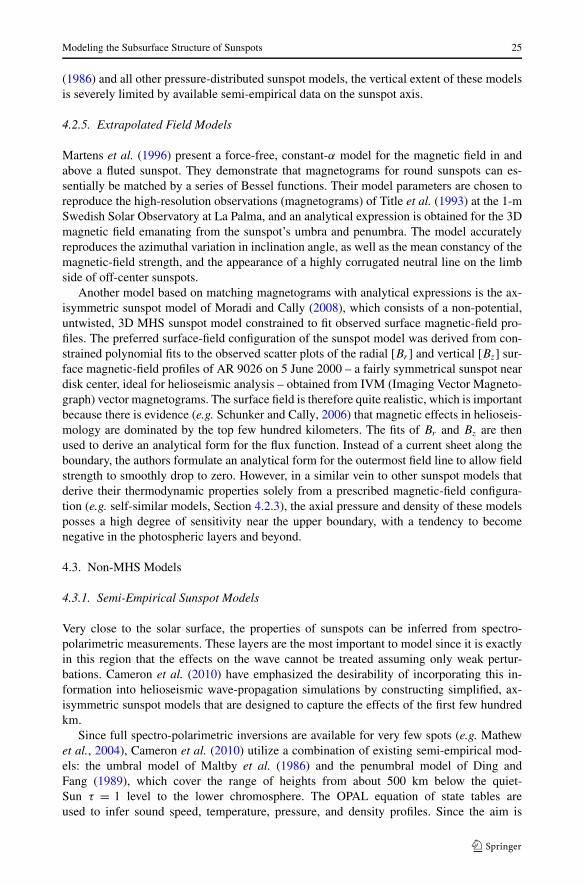
Modeling the Subsurface Structure of Sunspots 25
(1986) and all other pressure-distributed sunspot models, the vertical extent of these modelsis severely limited by available semi-empirical data on the sunspot axis.
4.2.5. Extrapolated Field Models
Martens et al. (1996) present a force-free, constant-α model for the magnetic field in andabove a fluted sunspot. They demonstrate that magnetograms for round sunspots can es-sentially be matched by a series of Bessel functions. Their model parameters are chosen toreproduce the high-resolution observations (magnetograms) of Title et al. (1993) at the 1-mSwedish Solar Observatory at La Palma, and an analytical expression is obtained for the 3Dmagnetic field emanating from the sunspot’s umbra and penumbra. The model accuratelyreproduces the azimuthal variation in inclination angle, as well as the mean constancy of themagnetic-field strength, and the appearance of a highly corrugated neutral line on the limbside of off-center sunspots.
Another model based on matching magnetograms with analytical expressions is the ax-isymmetric sunspot model of Moradi and Cally (2008), which consists of a non-potential,untwisted, 3D MHS sunspot model constrained to fit observed surface magnetic-field pro-files. The preferred surface-field configuration of the sunspot model was derived from con-strained polynomial fits to the observed scatter plots of the radial [Br ] and vertical [Bz] sur-face magnetic-field profiles of AR 9026 on 5 June 2000 – a fairly symmetrical sunspot neardisk center, ideal for helioseismic analysis – obtained from IVM (Imaging Vector Magneto-graph) vector magnetograms. The surface field is therefore quite realistic, which is importantbecause there is evidence (e.g. Schunker and Cally, 2006) that magnetic effects in helioseis-mology are dominated by the top few hundred kilometers. The fits of Br and Bz are thenused to derive an analytical form for the flux function. Instead of a current sheet along theboundary, the authors formulate an analytical form for the outermost field line to allow fieldstrength to smoothly drop to zero. However, in a similar vein to other sunspot models thatderive their thermodynamic properties solely from a prescribed magnetic-field configura-tion (e.g. self-similar models, Section 4.2.3), the axial pressure and density of these modelsposses a high degree of sensitivity near the upper boundary, with a tendency to becomenegative in the photospheric layers and beyond.
4.3. Non-MHS Models
4.3.1. Semi-Empirical Sunspot Models
Very close to the solar surface, the properties of sunspots can be inferred from spectro-polarimetric measurements. These layers are the most important to model since it is exactlyin this region that the effects on the wave cannot be treated assuming only weak pertur-bations. Cameron et al. (2010) have emphasized the desirability of incorporating this in-formation into helioseismic wave-propagation simulations by constructing simplified, ax-isymmetric sunspot models that are designed to capture the effects of the first few hundredkm.
Since full spectro-polarimetric inversions are available for very few spots (e.g. Mathewet al., 2004), Cameron et al. (2010) utilize a combination of existing semi-empirical mod-els: the umbral model of Maltby et al. (1986) and the penumbral model of Ding andFang (1989), which cover the range of heights from about 500 km below the quiet-Sun τ = 1 level to the lower chromosphere. The OPAL equation of state tables areused to infer sound speed, temperature, pressure, and density profiles. Since the aim is
26 H. Moradi et al.
Figure 3 Thermodynamic, sound and fast mode speed profiles of the sunspot model of AR 9787 producedby Cameron et al. (2010). Left panel: Vertical temperature profile of reference stratification (solid) and nearthe center of the umbra (dashed). Right panel: Vertical sound-speed profile of reference stratification (solid)and near the center of the umbra (dashed). The dotted line shows the fast-mode speed in the center of theumbra.
only to model the near-surface region, the atmospheric models are smoothly matched tothe Model S (Christensen-Dalsgaard et al., 1996) quiet-Sun atmosphere below τ5000 = 0and 400 km above. Cameron et al. (2010) combine these 1D models to form a 3D,axisymmetric model of the sunspot in AR 9787, with the umbral and penumbral radiichosen to match those of the observed sunspot (10 and 20 Mm, respectively). Themodel is then stabilized with respect to convection by calculating the relative pertur-bations with respect to the quiet-Sun atmosphere and imposing these on the stabilizedmodel (see Section 6.2 for details). As good measurements of the magnetic field areunavailable for the sunspot in AR 9787, the model assumes that Bz is described by aGaussian horizontal profile and the vertical profile is tuned so the field inclination atthe umbra – penumbra border is approximately 45°. Figure 3 shows the vertical temper-ature, sound and fast mode speed profiles in the center of the umbra of the sunspotmodel.
4.3.2. Dynamical Models
Kitchatinov and Rüdiger (2007) propose a theoretical sunspot model, with complete dynam-ics of both magnetic field and flow, which can reproduce the observed bright rings aroundsunspots (e.g. Rast et al., 1999, 2001). A simplified model was initially used to probe thepossibility of reproducing bright rings by heat transport alone. In this model the mean flowvelocity is put to zero, the spot-like structure of the magnetic field is prescribed and station-ary, and the diffusion equation for the entropy is solved. The authors find that the bright-ness of the region occupied by magnetic field decreases due to magnetic quenching of thethermal diffusivity; however, the resulting surface brightness profile did not show a brightring.
A more consistent MHD model of a sunspot was then considered using the completemomentum equation together with the induction equation. Amplitudes of the initial uniformfield of several hundred Gauss were considered. The surface flow generated is convergentnear the spot but divergent at larger distances. The amplitude of the flow modeled was ap-proximately 800 m s−1. Both brightness and field strength (central value of about 2700 G)
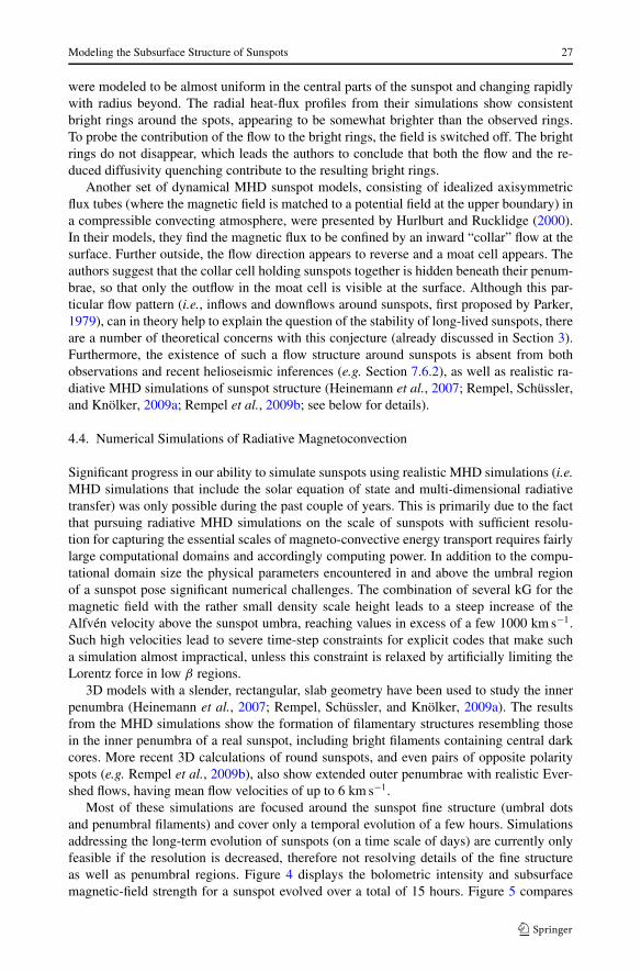
Modeling the Subsurface Structure of Sunspots 27
were modeled to be almost uniform in the central parts of the sunspot and changing rapidlywith radius beyond. The radial heat-flux profiles from their simulations show consistentbright rings around the spots, appearing to be somewhat brighter than the observed rings.To probe the contribution of the flow to the bright rings, the field is switched off. The brightrings do not disappear, which leads the authors to conclude that both the flow and the re-duced diffusivity quenching contribute to the resulting bright rings.
Another set of dynamical MHD sunspot models, consisting of idealized axisymmetricflux tubes (where the magnetic field is matched to a potential field at the upper boundary) ina compressible convecting atmosphere, were presented by Hurlburt and Rucklidge (2000).In their models, they find the magnetic flux to be confined by an inward “collar” flow at thesurface. Further outside, the flow direction appears to reverse and a moat cell appears. Theauthors suggest that the collar cell holding sunspots together is hidden beneath their penum-brae, so that only the outflow in the moat cell is visible at the surface. Although this par-ticular flow pattern (i.e., inflows and downflows around sunspots, first proposed by Parker,1979), can in theory help to explain the question of the stability of long-lived sunspots, thereare a number of theoretical concerns with this conjecture (already discussed in Section 3).Furthermore, the existence of such a flow structure around sunspots is absent from bothobservations and recent helioseismic inferences (e.g. Section 7.6.2), as well as realistic ra-diative MHD simulations of sunspot structure (Heinemann et al., 2007; Rempel, Schüssler,and Knölker, 2009a; Rempel et al., 2009b; see below for details).
4.4. Numerical Simulations of Radiative Magnetoconvection
Significant progress in our ability to simulate sunspots using realistic MHD simulations (i.e.MHD simulations that include the solar equation of state and multi-dimensional radiativetransfer) was only possible during the past couple of years. This is primarily due to the factthat pursuing radiative MHD simulations on the scale of sunspots with sufficient resolu-tion for capturing the essential scales of magneto-convective energy transport requires fairlylarge computational domains and accordingly computing power. In addition to the compu-tational domain size the physical parameters encountered in and above the umbral regionof a sunspot pose significant numerical challenges. The combination of several kG for themagnetic field with the rather small density scale height leads to a steep increase of theAlfvén velocity above the sunspot umbra, reaching values in excess of a few 1000 km s−1.Such high velocities lead to severe time-step constraints for explicit codes that make sucha simulation almost impractical, unless this constraint is relaxed by artificially limiting theLorentz force in low β regions.
3D models with a slender, rectangular, slab geometry have been used to study the innerpenumbra (Heinemann et al., 2007; Rempel, Schüssler, and Knölker, 2009a). The resultsfrom the MHD simulations show the formation of filamentary structures resembling thosein the inner penumbra of a real sunspot, including bright filaments containing central darkcores. More recent 3D calculations of round sunspots, and even pairs of opposite polarityspots (e.g. Rempel et al., 2009b), also show extended outer penumbrae with realistic Ever-shed flows, having mean flow velocities of up to 6 km s−1.
Most of these simulations are focused around the sunspot fine structure (umbral dotsand penumbral filaments) and cover only a temporal evolution of a few hours. Simulationsaddressing the long-term evolution of sunspots (on a time scale of days) are currently onlyfeasible if the resolution is decreased, therefore not resolving details of the fine structureas well as penumbral regions. Figure 4 displays the bolometric intensity and subsurfacemagnetic-field strength for a sunspot evolved over a total of 15 hours. Figure 5 compares
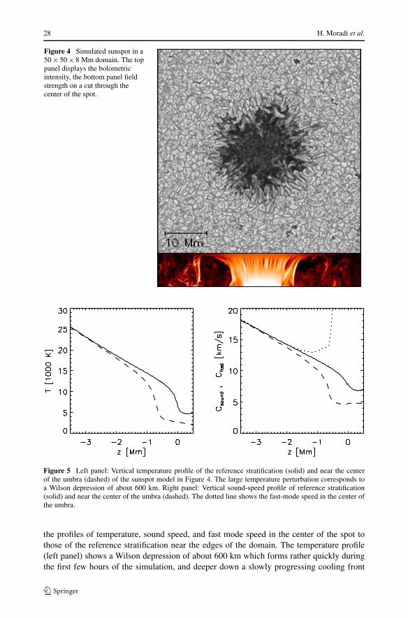
28 H. Moradi et al.
Figure 4 Simulated sunspot in a50 × 50 × 8 Mm domain. The toppanel displays the bolometricintensity, the bottom panel fieldstrength on a cut through thecenter of the spot.
Figure 5 Left panel: Vertical temperature profile of the reference stratification (solid) and near the centerof the umbra (dashed) of the sunspot model in Figure 4. The large temperature perturbation corresponds toa Wilson depression of about 600 km. Right panel: Vertical sound-speed profile of reference stratification(solid) and near the center of the umbra (dashed). The dotted line shows the fast-mode speed in the center ofthe umbra.
the profiles of temperature, sound speed, and fast mode speed in the center of the spot tothose of the reference stratification near the edges of the domain. The temperature profile(left panel) shows a Wilson depression of about 600 km which forms rather quickly duringthe first few hours of the simulation, and deeper down a slowly progressing cooling front
Modeling the Subsurface Structure of Sunspots 29
leads to a moderate adjustment of temperature in layers 1 – 2 Mm beneath the τ = 1 levelin the umbra corresponding to changes of the speed of sound (right panel) on the order ofa few 100 m s−1 to about 1 km s−1. The fast-mode speed shows a steep increase above theτ = 1 level in the umbra, the maximum speed is here artificially limited to about 60 km s−1
to relax the stringent Alfvénic time-step constraint.While these simulations provide a realistic description of the thermal and magnetic struc-
ture in the uppermost few Mm of a sunspot, they cannot address fundamental questions re-garding the subsurface structure and origin of sunspots. Currently the domains are with 8Mm still rather shallow (deeper domains up to 16 Mm are in preparation) and the initialfield structure is based on a monolithic model. Furthermore the magnetic field is fixed at thebottom boundary. Nevertheless these models provide very useful artificial oscillation datathat can be used to test helioseismic inversion methods, since the latter requires primarily aconsistent, rather than a fully realistic model.
5. Diagnostics Potential of Helioseismology
In the previous section we reviewed models of sunspots; each of these provides a prescrip-tion for computing the subsurface structure (i.e. the 3D forms of the sound speed, density,and magnetic field) of a model sunspot over some range of depths. These prescriptions arebased on a wide variety of physical assumptions. In general, it is not known which of theseassumptions are good approximations (in the sense of accurately describing solar condi-tions). Helioseismology promises the ability to infer the subsurface structure of sunspotsand active regions, and thus to test the physical approximations that are used in buildingmodels of these regions.
Helioseismology has shown (see Gizon and Birch, 2005 for a review) that wave prop-agation is different in sunspots in the quiet Sun. For example, single-bounce wave traveltimes are altered by (order of magnitude) about thirty seconds; the details depend stronglyon the data-analysis filters, the first-bounce distance, and the wave frequency (e.g. Braunand Birch, 2008). In Section 7 we provide a follow-up to the detailed helioseismic study un-dertaken by Gizon et al. (2009a, 2009b) of the active region AR 9787. These measurementsclearly demonstrate that helioseismology can measure the changes in wave propagation thatare associated with sunspots and active regions.
Many conclutions have been drawn about sunspot and active-region structure from lo-cal helioseismology (e.g. Fan, Braun, and Chou, 1995; Kosovichev, 1996; Jensen, Jacob-sen, and Christensen-Dalsgaard, 1998; Chou, Sun, and Chang, 2000; Kosovichev, Duvall,and Scherrer, 2000; Zhao and Kosovichev, 2003; Couvidat et al., 2004; Basu, Antia, andBogart, 2004; Crouch et al., 2005; Bogart et al., 2008). Despite the long history of workon this topic, there is no general agreement on the subsurface structure of active regions.Here we will investigate some of the possible causes of the disagreement shown by Gizonet al. (2009a, 2009b): the frequency dependence of travel times (Section 7.2), the effectsof phase-speed filters on measurements (Section 7.3), and the effects of inversion para-meter choices and inclusion of surface terms on ring-diagram structure inversions (Sec-tion 7.4).
Another approach to using helioseismology to constrain sunspot models is the directsimulation of wave propagation through model sunspots and comparison of the resultingwave field with the helioseismic measurements (e.g. Cameron, Gizon, and Daiffallah, 2007;Cameron, Gizon, and Duvall, 2008; Moradi, Hanasoge, and Cally, 2009). This approach by-passes the need for linear forward models (i.e. models for the linear sensitivity of travel-time
30 H. Moradi et al.
shifts or ring-diagram frequency shifts to changes in subsurface structure). The approxima-tions made in the process of formulating linear forward models may be one source of thedisagreement shown by Gizon et al. (2009a, 2009b). A limitation of the direct simulation ap-proach is that it is extremely computationally intensive. The examples shown in Section 7.8demonstrate that numerical simulations are capable of reproducing many features of thehelioseismic measurements (see also Cameron, Gizon, and Duvall, 2008). In addition, sim-ulations promise to provide a powerful tool for determining the sensitivity of helioseismicmeasurements to small changes in the subsurface structure of sunspot models. This typeof study is required to be able to make meaningful estimates of the signal-to-noise ratiosrequired for the helioseismic measurements to constrain any particular aspect of sunspotmodels.
6. Numerical Forward Modeling of Waves Through Model Sunspots
6.1. Numerical Methods
Our best chance at constraining the interior structure of sunspots comes with constructingaccurate, numerical, forward models. There are two major reasons for claiming this:
i) The departure from the quiet-Sun wave-propagation physics being so dramatic in asunspot, it is quite likely that the single-scattering Born approximation (e.g. Birch, Koso-vichev, and Duvall, 2004) fails entirely (e.g. Gizon, Hanasoge, and Birch, 2006). It istherefore imperative to solve the wave-propagation equations in a fully 3D, highly mag-netized environment. However, the basis of semi-analytical sunspot formalisms is sig-nificantly undermined by the sheer mathematical complexity of dealing with the MHDequations (not for the want of trying; e.g. Bogdan, 1999), and hence the necessity ofusing purely numerical techniques.
ii) Computational solvers are flexible and can be rather easily extended to include moreeffects, such as flows, changes on wave sources, etc.
The difficulties in creating an MHD solver that produces sufficiently accurate results arenot to be underestimated. A number of groups are working on this problem (Khomenko andCollados, 2006; Cameron, Gizon, and Daiffallah, 2007; Parchevsky and Kosovichev, 2007;Hanasoge, 2008; Shelyag et al., 2009). The numerical techniques, and validation and ver-ification procedures vary significantly from one code to another. A further complexity isintroduced by an Alfvén speed that increases exponentially with height, approaching valuesof several hundred km s−1 near the computational upper boundary. Simulating wave prop-agation in a plasma so highly magnetically dominated is remarkably expensive, especiallyin 3D. A number of simulations (e.g. Cameron, Gizon, and Daiffallah, 2007; Cameron,Gizon, and Duvall, 2008; Hanasoge, 2008; Moradi, Hanasoge, and Cally, 2009; Rempel,Schüssler, and Knölker, 2009a) apply an Alfvén wave-speed limiter to moderate the ac-tion of the Lorentz forces, thereby indirectly controlling the plasma-β . Having describedthis context, three rather serious issues remain as yet outstanding: i) What are the spatio-temporal resolution requirements for simulating waves in an MHD environment? ii) Howdo we treat the upper magnetic boundary? and iii) What harm does the Alfvén-speed limit-ing term do to the near and far scattered wave field?
As yet, only parts of these questions have been answered. This may be attributedto a systemic shortsighted forward modeling approach in our intensely observationallydriven field: simulate and obtain results as quickly as possible. Evidently, we must at-tempt to overturn this trend by i) ensuring that the numerical methods are high order
Modeling the Subsurface Structure of Sunspots 31
and highly precise, ii) validating and verifying that the equations are being solved accu-rately (i.e. testing against a number of known solutions), iii) determining and matchingthe spatio-temporal resolution requirements, iv) using stable, physically-motivated, well-tested boundary conditions, and finally v) testing that the approximations used in the cal-culations do not directly affect the quality of the solution. Of course, attendant questionsof computational efficiency must also be addressed, because the forward-modeling ap-proach requires exhaustive testing of sunspot models, requiring a large number of calcu-lations.
6.2. Background Models Stabilized Against Convective Instability
Numerical simulations of seismic wave propagation through random media must begin withan initial background model of the Sun. In helioseismology, it is common practice to be-gin with Model S (e.g. Cameron, Gizon, and Daiffallah, 2007; Parchevsky and Kosovichev,2007; Khomenko et al., 2009). However, most background models include convection andnumerical forward models which simulate linear wave propagation are sensitive to this.Therefore, it is essential to remove such convective instabilities from the background in or-der to be able to successfully simulate linear wave propagation on the time scalesk (≈ eighthours) required for computational helioseismology, as well as to ensure that convectivemodes do not swamp the signatures one is interested in analyzing.
There are a number of ways to stabilize background models against convection (e.g.Hanasoge et al., 2006; Cameron, Gizon, and Daiffallah, 2007; Parchevsky and Kosovichev,2007; Shelyag, Fedun, and Erdélyi, 2008), all requiring zero buoyancy so that a verticallydisplaced packet of gas in adiabatic equilibrium will not continue to rise, i.e. ensuring thatthe Brunt–Väisälä frequency always remains positive, specifically N2/g > 0 where g is thegravitational acceleration. There are a number of ways to go about this; for example, themethod employed by Parchevsky and Kosovichev (2007) ensures that, when this conditionis not met, the value is replaced with zero, or very small values (e.g. 3 × 10⁻⁵ Mm−1).Shelyag, Fedun, and Erdélyi (2008) and Shelyag et al. (2009) have a slightly different ap-proach, whereby they adjust the pressure and density of Model S using the equation of statefor an ideal gas to retain a constant �1 = 5/3, with the additional constraint that the mod-ified sound-speed profile does not differ substantially from the original. Both Parchevskyand Kosovichev (2007) and Shelyag et al. (2009) have shown relatively solar-like powerspectrums.
Another method has been employed by Cameron, Gizon, and Daiffallah (2007) andCameron, Gizon, and Duvall (2008), and it has undergone detailed development and testingby Schunker, Cameron, and Gizon (2010), whereby the Model S background is stabilizedagainst convective instability by ensuring ∂zp = max(c2∂zρ0 − ε, ∂zp0), where ∂z specifiesthe partial derivative with respect to height, the subscript “0” indicates unperturbed Model Svalues, and ε = 10−5 g s−2 near the surface and zero everywhere else. These changes tothe background model alter the eigenmodes of the problem, and this must be taken into ac-count. Schunker, Cameron, and Gizon (2010) have attempted to do this by examining theeigenmodes and ensuring that they are solar-like and have successfully demonstrated quitesolar-like power spectra. Other ways to remove the convective instability have not been ex-plored however, and it is not clear which form of stabilization least affects the eigenmodes.
6.3. Numerical Codes
In this section we provide a brief summary of the four numerical simulation codes that werediscussed and used during the two HELAS workshops on sunspot seismology held in 2007
32 H. Moradi et al.
and 2009. These codes compute the propagation of solar waves through prescribed back-ground models. We note that other numerical simulation codes also exist (e.g. Parchevskyand Kosovichev, 2007; Hartlep, Miesch, and Mansour, 2008).
6.3.1. The IAC MHD Code
The IAC MHD code, described by Khomenko and Collados (2006) and Khomenko, Col-lados, and Felipe (2008), solves the non-linear MHD equations for perturbations, writtenin the conservative form, using a fourth-order central difference scheme and advanced intime by a fourth-order Runge – Kutta method. In a similar manner to Stein and Nordlund(1998) and Caunt and Korpi (2001), in order to damp high-frequency numerical noise onsubgrid scales, the physical diffusive terms in the equations of momentum and energy arereplaced by artificial equivalents. In the induction equation, the magnetic-diffusion term isretained, with η being replaced by an artificial value. Depending on the simulation, PerfectlyMatched Layers (PML: e.g. Berenger, 1994) are also placed at the boundaries that absorbthe incoming waves and prevent their spurious reflection and return back to the physicaldomain. For the best results, 10 to 15 grid points are allocated to the PML layer. This codehas been used to study the wave propagation and refraction in a small sunspot (Khomenkoand Collados, 2006); non-linear wave propagation, shock formation, mode conversion, andenergy transport in small-scale flux tubes with internal structure (Khomenko, Collados, andFelipe, 2008).
Recently, the code was also used to model the propagation of helioseismic waves belowthe subphotospheric structure of sunspots (Khomenko et al., 2009; Khomenko and Colla-dos, 2009). The most important results obtained for helioseismic wave propagation belowsunspots are the following: i) the fast magnetoacoustic mode represents an analog of quiet-Sun p modes modified by the presence of magnetic field, ii) helioseismic waves belowsunspots are sped up by the magnetic field by 20 – 40 seconds compared to the quiet Sun,iii) the magnetic field produces a strong frequency dependence of the travel times, iv) theeikonal solution gives a qualitatively good approximation for the numerical solution, andfinally, v) the high-frequency fast-mode waves are refracted in the magnetically dominatedlayers and inject additional energy, possibly causing the power increase observed in acoustichalos surrounding active regions.
6.3.2. The SLiM Code
The Semispectral Linear MHD (SLiM) code solves the ideal linearized MHD equations us-ing a spectral expansion in the horizontal directions and a two-step Lax – Wendroff treatmentin the vertical. The code includes two absorbing layers at the top and the bottom of the box.In the top layer the waves are heavily damped and the effect of the Lorentz force is system-atically reduced. Likewise the bottom layer damps the waves that propagate downward. Thecode has been tested against analytic solutions, which are described in detail in Cameron,Gizon, and Daiffallah (2007).
In Cameron, Gizon, and Duvall (2008) and Gizon et al. (2009a, 2009b), SLiM was used tostudy wave propagation through a simplified monolithic model sunspot embedded in a sta-bilized quiet-Sun model atmosphere (see Section 6.2). The corresponding wave field com-puted with SLiM was then compared with MDI observations of f - and p-mode scatteringby the sunspot in AR 9787. The comparisons were quite encouraging as the numerical sim-ulations from SLiM were able to reproduce wave absorption and scattering phase shifts. Thecode has also recently been used on the sunspot model described in Section 4.3.1, as well as
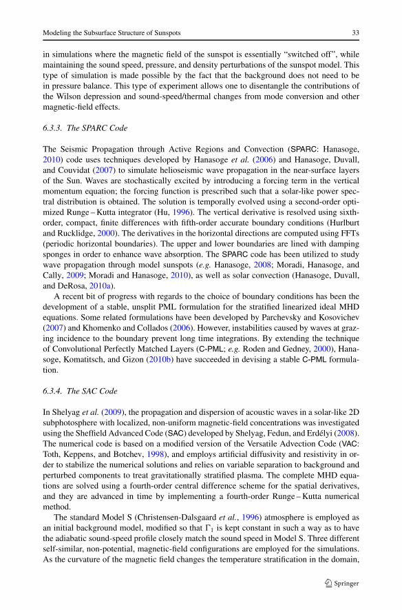
Modeling the Subsurface Structure of Sunspots 33
in simulations where the magnetic field of the sunspot is essentially “switched off”, whilemaintaining the sound speed, pressure, and density perturbations of the sunspot model. Thistype of simulation is made possible by the fact that the background does not need to bein pressure balance. This type of experiment allows one to disentangle the contributions ofthe Wilson depression and sound-speed/thermal changes from mode conversion and othermagnetic-field effects.
6.3.3. The SPARC Code
The Seismic Propagation through Active Regions and Convection (SPARC: Hanasoge,2010) code uses techniques developed by Hanasoge et al. (2006) and Hanasoge, Duvall,and Couvidat (2007) to simulate helioseismic wave propagation in the near-surface layersof the Sun. Waves are stochastically excited by introducing a forcing term in the verticalmomentum equation; the forcing function is prescribed such that a solar-like power spec-tral distribution is obtained. The solution is temporally evolved using a second-order opti-mized Runge – Kutta integrator (Hu, 1996). The vertical derivative is resolved using sixth-order, compact, finite differences with fifth-order accurate boundary conditions (Hurlburtand Rucklidge, 2000). The derivatives in the horizontal directions are computed using FFTs(periodic horizontal boundaries). The upper and lower boundaries are lined with dampingsponges in order to enhance wave absorption. The SPARC code has been utilized to studywave propagation through model sunspots (e.g. Hanasoge, 2008; Moradi, Hanasoge, andCally, 2009; Moradi and Hanasoge, 2010), as well as solar convection (Hanasoge, Duvall,and DeRosa, 2010a).
A recent bit of progress with regards to the choice of boundary conditions has been thedevelopment of a stable, unsplit PML formulation for the stratified linearized ideal MHDequations. Some related formulations have been developed by Parchevsky and Kosovichev(2007) and Khomenko and Collados (2006). However, instabilities caused by waves at graz-ing incidence to the boundary prevent long time integrations. By extending the techniqueof Convolutional Perfectly Matched Layers (C-PML; e.g. Roden and Gedney, 2000), Hana-soge, Komatitsch, and Gizon (2010b) have succeeded in devising a stable C-PML formula-tion.
6.3.4. The SAC Code
In Shelyag et al. (2009), the propagation and dispersion of acoustic waves in a solar-like 2Dsubphotosphere with localized, non-uniform magnetic-field concentrations was investigatedusing the Sheffield Advanced Code (SAC) developed by Shelyag, Fedun, and Erdélyi (2008).The numerical code is based on a modified version of the Versatile Advection Code (VAC:Toth, Keppens, and Botchev, 1998), and employs artificial diffusivity and resistivity in or-der to stabilize the numerical solutions and relies on variable separation to background andperturbed components to treat gravitationally stratified plasma. The complete MHD equa-tions are solved using a fourth-order central difference scheme for the spatial derivatives,and they are advanced in time by implementing a fourth-order Runge – Kutta numericalmethod.
The standard Model S (Christensen-Dalsgaard et al., 1996) atmosphere is employed asan initial background model, modified so that �1 is kept constant in such a way as to havethe adiabatic sound-speed profile closely match the sound speed in Model S. Three differentself-similar, non-potential, magnetic-field configurations are employed for the simulations.As the curvature of the magnetic field changes the temperature stratification in the domain,
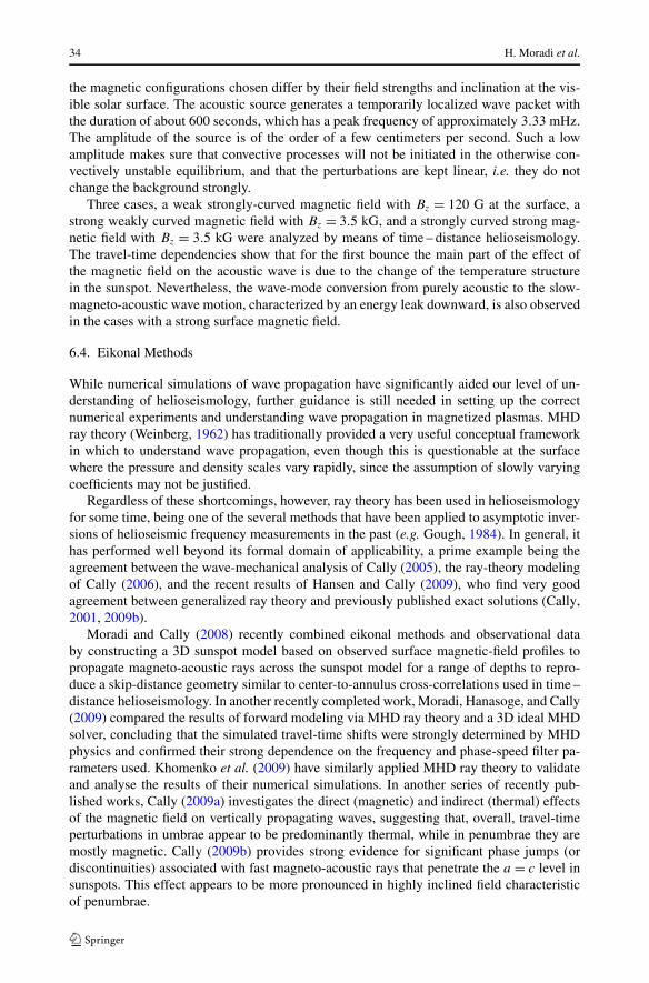
34 H. Moradi et al.
the magnetic configurations chosen differ by their field strengths and inclination at the vis-ible solar surface. The acoustic source generates a temporarily localized wave packet withthe duration of about 600 seconds, which has a peak frequency of approximately 3.33 mHz.The amplitude of the source is of the order of a few centimeters per second. Such a lowamplitude makes sure that convective processes will not be initiated in the otherwise con-vectively unstable equilibrium, and that the perturbations are kept linear, i.e. they do notchange the background strongly.
Three cases, a weak strongly-curved magnetic field with Bz = 120 G at the surface, astrong weakly curved magnetic field with Bz = 3.5 kG, and a strongly curved strong mag-netic field with Bz = 3.5 kG were analyzed by means of time – distance helioseismology.The travel-time dependencies show that for the first bounce the main part of the effect ofthe magnetic field on the acoustic wave is due to the change of the temperature structurein the sunspot. Nevertheless, the wave-mode conversion from purely acoustic to the slow-magneto-acoustic wave motion, characterized by an energy leak downward, is also observedin the cases with a strong surface magnetic field.
6.4. Eikonal Methods
While numerical simulations of wave propagation have significantly aided our level of un-derstanding of helioseismology, further guidance is still needed in setting up the correctnumerical experiments and understanding wave propagation in magnetized plasmas. MHDray theory (Weinberg, 1962) has traditionally provided a very useful conceptual frameworkin which to understand wave propagation, even though this is questionable at the surfacewhere the pressure and density scales vary rapidly, since the assumption of slowly varyingcoefficients may not be justified.
Regardless of these shortcomings, however, ray theory has been used in helioseismologyfor some time, being one of the several methods that have been applied to asymptotic inver-sions of helioseismic frequency measurements in the past (e.g. Gough, 1984). In general, ithas performed well beyond its formal domain of applicability, a prime example being theagreement between the wave-mechanical analysis of Cally (2005), the ray-theory modelingof Cally (2006), and the recent results of Hansen and Cally (2009), who find very goodagreement between generalized ray theory and previously published exact solutions (Cally,2001, 2009b).
Moradi and Cally (2008) recently combined eikonal methods and observational databy constructing a 3D sunspot model based on observed surface magnetic-field profiles topropagate magneto-acoustic rays across the sunspot model for a range of depths to repro-duce a skip-distance geometry similar to center-to-annulus cross-correlations used in time –distance helioseismology. In another recently completed work, Moradi, Hanasoge, and Cally(2009) compared the results of forward modeling via MHD ray theory and a 3D ideal MHDsolver, concluding that the simulated travel-time shifts were strongly determined by MHDphysics and confirmed their strong dependence on the frequency and phase-speed filter pa-rameters used. Khomenko et al. (2009) have similarly applied MHD ray theory to validateand analyse the results of their numerical simulations. In another series of recently pub-lished works, Cally (2009a) investigates the direct (magnetic) and indirect (thermal) effectsof the magnetic field on vertically propagating waves, suggesting that, overall, travel-timeperturbations in umbrae appear to be predominantly thermal, while in penumbrae they aremostly magnetic. Cally (2009b) provides strong evidence for significant phase jumps (ordiscontinuities) associated with fast magneto-acoustic rays that penetrate the a = c level insunspots. This effect appears to be more pronounced in highly inclined field characteristicof penumbrae.
Modeling the Subsurface Structure of Sunspots 35
Most of the above work has centered on the study of properties of individual rays prop-agating through magnetized atmosphere by solving the ray equations for a point source innon-magnetic solar model. In a recent study, Shelyag et al. (2009) have shown the impor-tance of considering the full family of rays corresponding to a particular problem’s initialconditions, as these define important geometric properties of the excited wave field such asthe wave front, caustics, and phase surfaces.
7. Update on the Analysis of AR 9787
7.1. Travel-Times Comparison: Time – Distance and Helioseismic Holography
It has been thought by some that travel times computed from time – distance helioseismology(Duvall et al., 1997) should be very similar (or maybe identical) to those measured usinghelioseismic holography (Braun and Lindsey, 2000). However, a detailed comparison ofmeasured travel times has not been done. We have done such a comparison for an eigh-hourinterval for AR 9787. For the time – distance case, correlations are calculated between thecentral point and the quadrants. For the holography, egression and ingression signals areconstructed in a quadrant geometry and correlations are done with the central point. Normalphase-speed filters were used (Couvidat et al., 2005).
Cuts across the travel-time maps for the sunspot are shown in Figure 6 for two dis-tances. Frames (a) and (b) show the distance 24.35 Mm and (c) and (d) show the short-est distance 6.20 Mm. The agreement is excellent for the distance of 24.35 Mm. How-ever, there are still disagreements for the shortest distances, which we hope to understandsoon.
7.2. Frequency Dependence of One-Way Travel Times
The dependence of mean and difference travel times on the central frequency of thewave packets measured over a sunspot region was shown and interpreted by Braun andBirch (2006, 2008) as an indication of perturbations largely confined to a region not deeperthan a few Mm. The largest frequency variations in travel times were seen for the smalltravel distances [ ] which are of the size (diameter) of the spot or smaller. In this sec-tion, we conduct a similar study for the sunspot in AR 9787. This type of study is impor-tant as, in principle, it should help us to constrain models of the subsurface structure ofsunspots.
Apart from a phase-speed filter centered around a phase speed vph = 54 km s−1 witha width (FWHM) of about 40% of vph, we also use Gaussian frequency filters, of 1-mHzwidth, centered at every 0.25-mHz interval between 2.5 and 5.0 mHz to study the frequencydependencies of the travel times. In Figure 7 we show the umbral averages of perturba-tions associated with in-going and out-going wave travel times (measured using center-to-annulus surface-focus geometry), δτin and δτout, as well as mean travel-time perturbations,δτmean, against frequency for = 50 Mm. There appears to be a strong frequency depen-dence associated with both δτin and δτout measured across the umbra of the sunspot in AR9787. This result appears to be in good qualitative agreement with the measurements ofBraun and Birch (2008), who look at frequency dependence of the travel-time difference,albeit for another sunspot. In particular, see the top right panel of Figure 5 in Braun andBirch (2008), which contains the travel-time difference results for Filter I (distances of 48 –55 Mm).
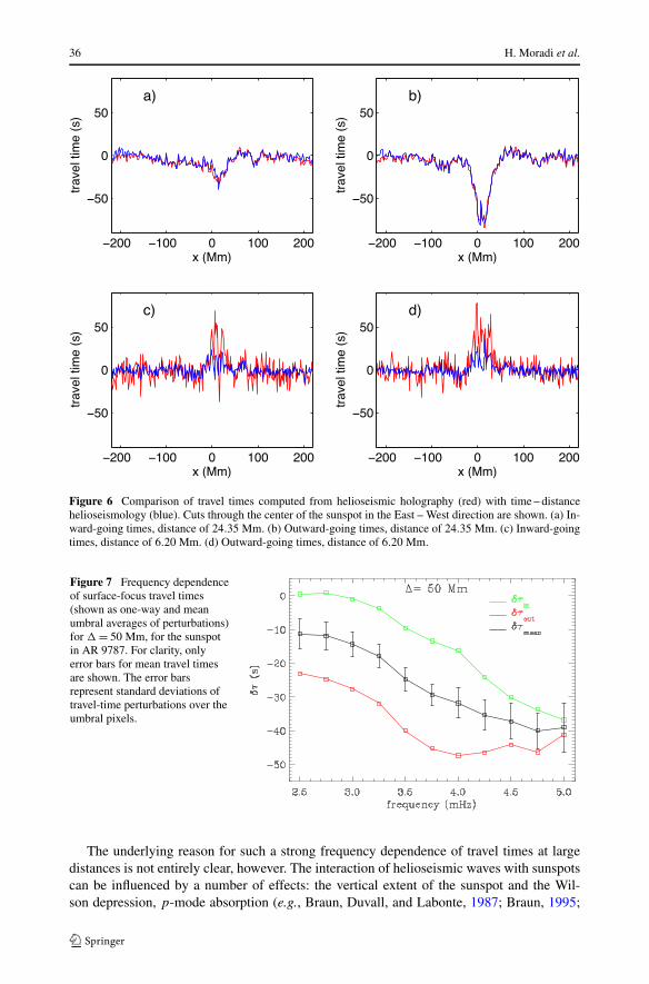
36 H. Moradi et al.
Figure 6 Comparison of travel times computed from helioseismic holography (red) with time – distancehelioseismology (blue). Cuts through the center of the sunspot in the East – West direction are shown. (a) In-ward-going times, distance of 24.35 Mm. (b) Outward-going times, distance of 24.35 Mm. (c) Inward-goingtimes, distance of 6.20 Mm. (d) Outward-going times, distance of 6.20 Mm.
Figure 7 Frequency dependenceof surface-focus travel times(shown as one-way and meanumbral averages of perturbations)for = 50 Mm, for the sunspotin AR 9787. For clarity, onlyerror bars for mean travel timesare shown. The error barsrepresent standard deviations oftravel-time perturbations over theumbral pixels.
The underlying reason for such a strong frequency dependence of travel times at largedistances is not entirely clear, however. The interaction of helioseismic waves with sunspotscan be influenced by a number of effects: the vertical extent of the sunspot and the Wil-son depression, p-mode absorption (e.g., Braun, Duvall, and Labonte, 1987; Braun, 1995;
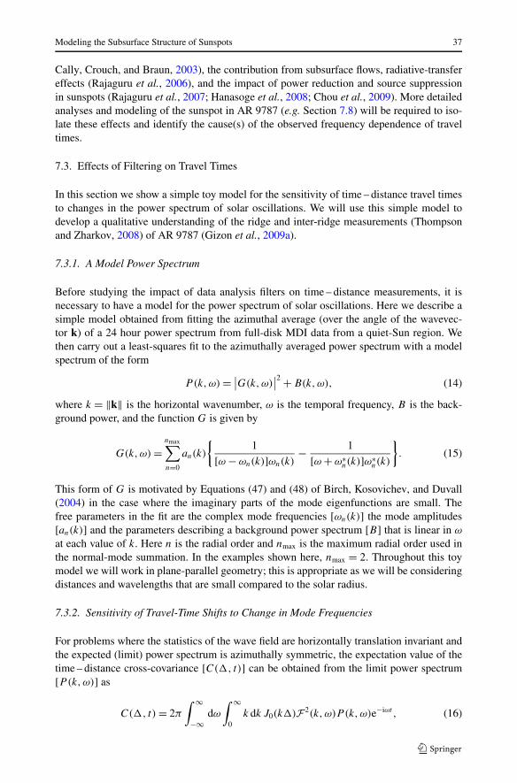
Modeling the Subsurface Structure of Sunspots 37
Cally, Crouch, and Braun, 2003), the contribution from subsurface flows, radiative-transfereffects (Rajaguru et al., 2006), and the impact of power reduction and source suppressionin sunspots (Rajaguru et al., 2007; Hanasoge et al., 2008; Chou et al., 2009). More detailedanalyses and modeling of the sunspot in AR 9787 (e.g. Section 7.8) will be required to iso-late these effects and identify the cause(s) of the observed frequency dependence of traveltimes.
7.3. Effects of Filtering on Travel Times
In this section we show a simple toy model for the sensitivity of time – distance travel timesto changes in the power spectrum of solar oscillations. We will use this simple model todevelop a qualitative understanding of the ridge and inter-ridge measurements (Thompsonand Zharkov, 2008) of AR 9787 (Gizon et al., 2009a).
7.3.1. A Model Power Spectrum
Before studying the impact of data analysis filters on time – distance measurements, it isnecessary to have a model for the power spectrum of solar oscillations. Here we describe asimple model obtained from fitting the azimuthal average (over the angle of the wavevec-tor k) of a 24 hour power spectrum from full-disk MDI data from a quiet-Sun region. Wethen carry out a least-squares fit to the azimuthally averaged power spectrum with a modelspectrum of the form
P (k,ω) = ∣∣G(k,ω)∣∣2 + B(k,ω), (14)
where k = ‖k‖ is the horizontal wavenumber, ω is the temporal frequency, B is the back-ground power, and the function G is given by
G(k,ω) =nmax∑n=0
an(k)
{1
[ω − ωn(k)]ωn(k)− 1
[ω + ω∗n(k)]ω∗
n(k)
}. (15)
This form of G is motivated by Equations (47) and (48) of Birch, Kosovichev, and Duvall(2004) in the case where the imaginary parts of the mode eigenfunctions are small. Thefree parameters in the fit are the complex mode frequencies [ωn(k)] the mode amplitudes[an(k)] and the parameters describing a background power spectrum [B] that is linear in ω
at each value of k. Here n is the radial order and nmax is the maximum radial order used inthe normal-mode summation. In the examples shown here, nmax = 2. Throughout this toymodel we will work in plane-parallel geometry; this is appropriate as we will be consideringdistances and wavelengths that are small compared to the solar radius.
7.3.2. Sensitivity of Travel-Time Shifts to Change in Mode Frequencies
For problems where the statistics of the wave field are horizontally translation invariant andthe expected (limit) power spectrum is azimuthally symmetric, the expectation value of thetime – distance cross-covariance [C( , t)] can be obtained from the limit power spectrum[P (k,ω)] as
C( , t) = 2π
∫ ∞
−∞dω
∫ ∞
0k dk J0(k )F 2(k,ω)P (k,ω)e−iωt , (16)
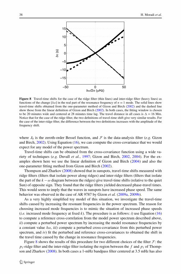
38 H. Moradi et al.
Figure 8 Travel-time shifts for the case of the ridge filter (thin lines) and inter-ridge filter (heavy lines) asfunctions of the change [δω] in the real part of the resonance frequency of n = 1 mode. The solid lines showtravel-time shifts obtained from the one-parameter method of Gizon and Birch (2002) and the dashed lineshow those from the linear definition of Gizon and Birch (2002). In both cases, the fitting window is chosento be 20 minutes wide and centered at 28 minutes time lag. The travel distance in all cases is = 16 Mm.Notice that for the case of the ridge filter, the two definitions of travel-time shift give very similar results. Forthe case of the inter-ridge filter, the difference between the two definitions increases with the amplitude of thefrequency shift.
where J0 is the zeroth-order Bessel function, and F is the data-analysis filter (e.g. Gizonand Birch, 2002). Using Equation (16), we can compute the cross-covariance that we wouldexpect for any model of the power spectrum.
Travel-time shifts can be obtained from the cross-covariance function using a wide va-riety of techniques (e.g. Duvall et al., 1997; Gizon and Birch, 2002, 2004). For the ex-amples shown here we use the linear definition of Gizon and Birch (2004) and also theone-parameter fitting method from Gizon and Birch (2002).
Thompson and Zharkov (2008) showed that in sunspots, travel-time shifts measured withridge filters (filters that isolate power along ridges) and inter-ridge filters (filters that isolatethe part of the k −ω diagram between the ridges) give travel-time shifts (relative to the quietSun) of opposite sign. They found that the ridge filters yielded decreased phase-travel times.This would seem to imply that the waves in sunspots have increased phase speed. The samebehavior was observed in the case of AR 9787 by Gizon et al. (2009a, 2009b).
As a very highly simplified toy model of this situation, we investigate the travel-timeshifts caused by increasing the resonant frequencies in the power spectrum. The reason forchoosing increased mode frequencies is to mimic the situation of increased phase speeds(i.e. increased mode frequency at fixed k). The procedure is as follows: i) use Equation (16)to compute a reference cross-correlation from the model power spectrum described above,ii) compute a perturbed power spectrum by increasing the model resonance frequencies bya constant value δω, iii) compute a perturbed cross-covariance from this perturbed powerspectrum, and iv) fit the perturbed and reference cross-covariances to obtained the shift inthe travel time caused by the change in resonance frequencies.
Figure 8 shows the results of this procedure for two different choices of the filter F : thep1-ridge filter and the inter-ridge filter isolating the region between the f and p1 of Thomp-son and Zharkov (2008). In both cases a 1-mHz bandpass filter centered at 3.5 mHz has also
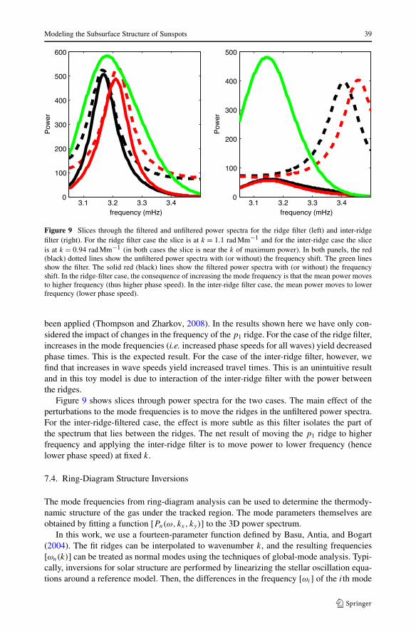
Modeling the Subsurface Structure of Sunspots 39
Figure 9 Slices through the filtered and unfiltered power spectra for the ridge filter (left) and inter-ridgefilter (right). For the ridge filter case the slice is at k = 1.1 rad Mm−1 and for the inter-ridge case the sliceis at k = 0.94 rad Mm−1 (in both cases the slice is near the k of maximum power). In both panels, the red(black) dotted lines show the unfiltered power spectra with (or without) the frequency shift. The green linesshow the filter. The solid red (black) lines show the filtered power spectra with (or without) the frequencyshift. In the ridge-filter case, the consequence of increasing the mode frequency is that the mean power movesto higher frequency (thus higher phase speed). In the inter-ridge filter case, the mean power moves to lowerfrequency (lower phase speed).
been applied (Thompson and Zharkov, 2008). In the results shown here we have only con-sidered the impact of changes in the frequency of the p1 ridge. For the case of the ridge filter,increases in the mode frequencies (i.e. increased phase speeds for all waves) yield decreasedphase times. This is the expected result. For the case of the inter-ridge filter, however, wefind that increases in wave speeds yield increased travel times. This is an unintuitive resultand in this toy model is due to interaction of the inter-ridge filter with the power betweenthe ridges.
Figure 9 shows slices through power spectra for the two cases. The main effect of theperturbations to the mode frequencies is to move the ridges in the unfiltered power spectra.For the inter-ridge-filtered case, the effect is more subtle as this filter isolates the part ofthe spectrum that lies between the ridges. The net result of moving the p1 ridge to higherfrequency and applying the inter-ridge filter is to move power to lower frequency (hencelower phase speed) at fixed k.
7.4. Ring-Diagram Structure Inversions
The mode frequencies from ring-diagram analysis can be used to determine the thermody-namic structure of the gas under the tracked region. The mode parameters themselves areobtained by fitting a function [Pn(ω, kx, ky)] to the 3D power spectrum.
In this work, we use a fourteen-parameter function defined by Basu, Antia, and Bogart(2004). The fit ridges can be interpolated to wavenumber k, and the resulting frequencies[ωn(k)] can be treated as normal modes using the techniques of global-mode analysis. Typi-cally, inversions for solar structure are performed by linearizing the stellar oscillation equa-tions around a reference model. Then, the differences in the frequency [ωi ] of the ith mode
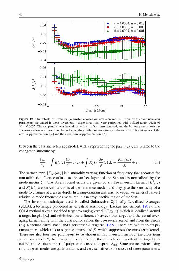
40 H. Moradi et al.
Figure 10 The effects of inversion-parameter choices on inversion results. Three of the four inversionparameters are varied in these inversions – these inversions were performed with a fixed target width ofW = 0.0055. The top panel shows inversions with a surface term removed, and the bottom panel shows in-versions without a surface term. In each case, three different inversions are shown with different values of theerror-suppression term [μ] and the cross-term suppression term [β].
between the data and reference model, with i representing the pair (n, k), are related to thechanges in structure by:
δωi
ωi
=∫
Ki
c2(z)δc2
c2(z) dz +
∫Ki
ρ(z)δρ
ρ(z) dz + Fsurf(ωi)
Qi
+ εi . (17)
The surface term [Fsurf(ωi)] is a smoothly varying function of frequency that accounts fornon-adiabatic effects confined to the surface layers of the Sun and is normalized by themode inertia Qi . The observational errors are given by εi . The inversion kernels [Ki
c2(z)
and Kiρ(z)] are known functions of the reference model, and they give the sensitivity of a
mode to changes at a given depth. In a ring-diagram analysis, however, we generally invertrelative to mode frequencies measured in a nearby inactive region of the Sun.
The inversion technique used is called Subtractive Optimally Localized Averages(SOLA), a technique pioneered in terrestrial seismology (Backus and Gilbert, 1967). TheSOLA method takes a specified target averaging kernel [T (z0, z)] which is localized arounda target height [z0] and minimizes the difference between that target and the actual aver-aging kernel, along with the contributions from the cross-term kernel and from the errors(e.g. Rabello-Soares, Basu, and Christensen-Dalsgaard, 1999). There are two trade-off pa-rameters: μ, which acts to suppress errors, and β , which suppresses the cross-term kernel.There are also four free parameters to be chosen in this inversion method: the cross-termsuppression term β , the error suppression term μ, the characteristic width of the target ker-nel W , and �, the number of polynomials used to expand Fsurf. Structure inversions usingring-diagram modes are quite unstable, and very sensitive to the choice of these parameters.
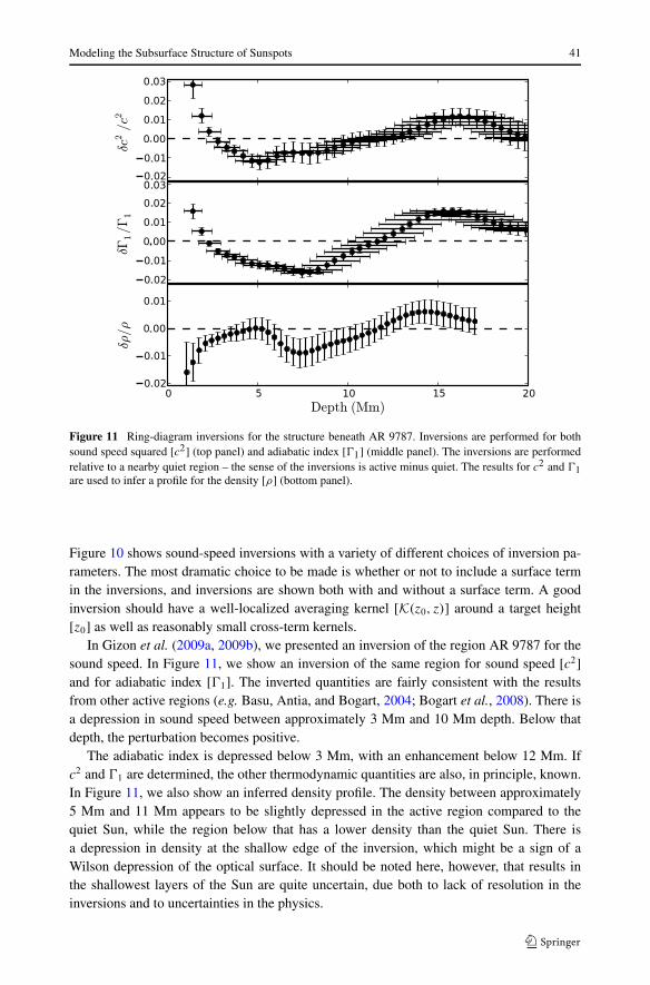
Modeling the Subsurface Structure of Sunspots 41
Figure 11 Ring-diagram inversions for the structure beneath AR 9787. Inversions are performed for bothsound speed squared [c2] (top panel) and adiabatic index [�1] (middle panel). The inversions are performedrelative to a nearby quiet region – the sense of the inversions is active minus quiet. The results for c2 and �1are used to infer a profile for the density [ρ] (bottom panel).
Figure 10 shows sound-speed inversions with a variety of different choices of inversion pa-rameters. The most dramatic choice to be made is whether or not to include a surface termin the inversions, and inversions are shown both with and without a surface term. A goodinversion should have a well-localized averaging kernel [K(z0, z)] around a target height[z0] as well as reasonably small cross-term kernels.
In Gizon et al. (2009a, 2009b), we presented an inversion of the region AR 9787 for thesound speed. In Figure 11, we show an inversion of the same region for sound speed [c2]and for adiabatic index [�1]. The inverted quantities are fairly consistent with the resultsfrom other active regions (e.g. Basu, Antia, and Bogart, 2004; Bogart et al., 2008). There isa depression in sound speed between approximately 3 Mm and 10 Mm depth. Below thatdepth, the perturbation becomes positive.
The adiabatic index is depressed below 3 Mm, with an enhancement below 12 Mm. Ifc2 and �1 are determined, the other thermodynamic quantities are also, in principle, known.In Figure 11, we also show an inferred density profile. The density between approximately5 Mm and 11 Mm appears to be slightly depressed in the active region compared to thequiet Sun, while the region below that has a lower density than the quiet Sun. There isa depression in density at the shallow edge of the inversion, which might be a sign of aWilson depression of the optical surface. It should be noted here, however, that results inthe shallowest layers of the Sun are quite uncertain, due both to lack of resolution in theinversions and to uncertainties in the physics.
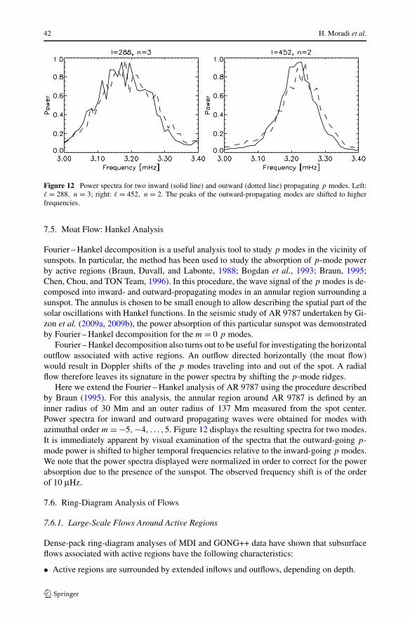
42 H. Moradi et al.
Figure 12 Power spectra for two inward (solid line) and outward (dotted line) propagating p modes. Left:� = 288, n = 3; right: � = 452, n = 2. The peaks of the outward-propagating modes are shifted to higherfrequencies.
7.5. Moat Flow: Hankel Analysis
Fourier – Hankel decomposition is a useful analysis tool to study p modes in the vicinity ofsunspots. In particular, the method has been used to study the absorption of p-mode powerby active regions (Braun, Duvall, and Labonte, 1988; Bogdan et al., 1993; Braun, 1995;Chen, Chou, and TON Team, 1996). In this procedure, the wave signal of the p modes is de-composed into inward- and outward-propagating modes in an annular region surrounding asunspot. The annulus is chosen to be small enough to allow describing the spatial part of thesolar oscillations with Hankel functions. In the seismic study of AR 9787 undertaken by Gi-zon et al. (2009a, 2009b), the power absorption of this particular sunspot was demonstratedby Fourier – Hankel decomposition for the m = 0 p modes.
Fourier – Hankel decomposition also turns out to be useful for investigating the horizontaloutflow associated with active regions. An outflow directed horizontally (the moat flow)would result in Doppler shifts of the p modes traveling into and out of the spot. A radialflow therefore leaves its signature in the power spectra by shifting the p-mode ridges.
Here we extend the Fourier – Hankel analysis of AR 9787 using the procedure describedby Braun (1995). For this analysis, the annular region around AR 9787 is defined by aninner radius of 30 Mm and an outer radius of 137 Mm measured from the spot center.Power spectra for inward and outward propagating waves were obtained for modes withazimuthal order m = −5,−4, . . . ,5. Figure 12 displays the resulting spectra for two modes.It is immediately apparent by visual examination of the spectra that the outward-going p-mode power is shifted to higher temporal frequencies relative to the inward-going p modes.We note that the power spectra displayed were normalized in order to correct for the powerabsorption due to the presence of the sunspot. The observed frequency shift is of the orderof 10 μHz.
7.6. Ring-Diagram Analysis of Flows
7.6.1. Large-Scale Flows Around Active Regions
Dense-pack ring-diagram analyses of MDI and GONG++ data have shown that subsurfaceflows associated with active regions have the following characteristics:
• Active regions are surrounded by extended inflows and outflows, depending on depth.
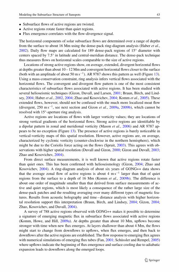
Modeling the Subsurface Structure of Sunspots 43
• Subsurface flows of active regions are twisted.• Active regions rotate faster than quiet regions.• Flux emergence correlates with the flow-divergence signal.
The horizontal components of solar subsurface flows are determined over a range of depthsfrom the surface to about 16 Mm using the dense-pack ring-diagram analysis (Haber et al.,2002). Daily flow maps are calculated for 189 dense-pack regions of 15° diameter withcenters spaced by 7.5° in latitude and central-meridian distance. The dense-pack techniquethus measures flows on horizontal scales comparable to the size of active regions.
Locations of strong active regions show, on average, extended, divergent horizontal flowsat depths greater than about 10 – 12 Mm and convergent horizontal flows closer to the surface(both with an amplitude of about 50 m s−1). AR 9787 shows this pattern as well (Figure 13).Using a mass-conservation constraint, ring analysis infers vertical flows associated with thehorizontal flows. The convergent and divergent flow pattern is one of the most consistentcharacteristics of subsurface flows associated with active regions. It has been studied withseveral helioseismic techniques (Gizon, Duvall, and Larsen, 2001; Braun, Birch, and Lind-sey, 2004; Haber et al., 2002, 2004; Zhao and Kosovichev, 2004; Komm et al., 2005). Theseextended flows, however, should not be confused with the much more localized moat flow(divergent, 250 m s−1, see next section and Gizon et al., 2009a, 2009b), which cannot beresolved with 15°-aperture ring analysis.
Active regions are locations of flows with larger vorticity values; they are locations ofstrong vertical gradients of the horizontal flows. Strong active regions are identifiable bya dipolar pattern in zonal and meridional vorticity (Mason et al., 2006) and AR 9787 ap-pears to be no exception (Figure 13). The presence of active regions is barely noticeable invertical-vorticity maps of this spatial resolution. However, active regions are, on average,characterized by cyclonic vorticity (counter-clockwise in the northern hemisphere), whichmight be due to the Coriolis force acting on the flows (Spruit, 2003). This agrees with ob-servations with higher spatial resolution (Duvall and Gizon, 2000; Gizon and Duvall, 2003;Zhao and Kosovichev, 2004).
From direct surface measurements, it is well known that active regions rotate fasterthan quiet ones. This has been confirmed with helioseismology (Gizon, 2004; Zhao andKosovichev, 2004). A ring-diagram analysis of about six years of GONG++ data showsthat the average zonal flow of active regions is about 4 m s−1 larger than that of quietregions from the surface to a depth of 16 Mm (Komm et al., 2009b). The difference isabout one order of magnitude smaller than that derived from surface measurements of ac-tive and quiet regions, which is most likely a consequence of the rather large size of thedense-pack patches and the resulting averaging over many different types of magnetic fea-tures. Results from acoustic holography and time – distance analysis with higher horizon-tal resolution support this interpretation (Braun, Birch, and Lindsey, 2004; Gizon, 2004;Zhao, Kosovichev, and Duvall, 2004).
A survey of 788 active regions observed with GONG++ makes it possible to determinea signature of emerging magnetic flux in subsurface flows associated with active regions(Komm, Howe, and Hill, 2009a). At depths greater than about 10 Mm, upflows becomestronger with time when new flux emerges. At layers shallower than about 4 Mm, the flowsmight start to change from downflows to upflows, when flux emerges, and then back todownflows after the active regions are established. The flow response to emerging flux agreeswith numerical simulations of emerging flux tubes (Fan, 2001; Schüssler and Rempel, 2005)where upflows indicate the beginning of flux emergence and surface cooling due to adiabaticexpansion leads to downflows along the emerged loops.
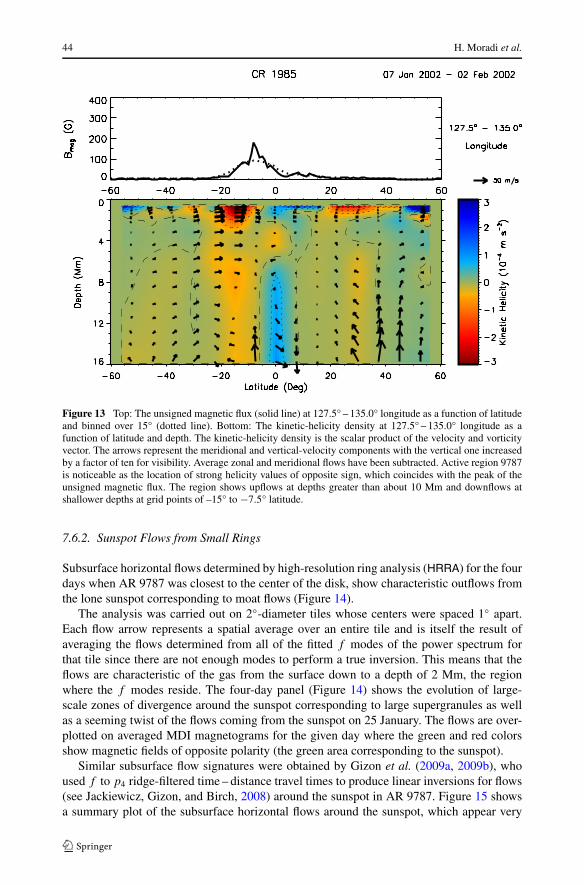
44 H. Moradi et al.
Figure 13 Top: The unsigned magnetic flux (solid line) at 127.5° – 135.0° longitude as a function of latitudeand binned over 15° (dotted line). Bottom: The kinetic-helicity density at 127.5° – 135.0° longitude as afunction of latitude and depth. The kinetic-helicity density is the scalar product of the velocity and vorticityvector. The arrows represent the meridional and vertical-velocity components with the vertical one increasedby a factor of ten for visibility. Average zonal and meridional flows have been subtracted. Active region 9787is noticeable as the location of strong helicity values of opposite sign, which coincides with the peak of theunsigned magnetic flux. The region shows upflows at depths greater than about 10 Mm and downflows atshallower depths at grid points of –15° to −7.5° latitude.
7.6.2. Sunspot Flows from Small Rings
Subsurface horizontal flows determined by high-resolution ring analysis (HRRA) for the fourdays when AR 9787 was closest to the center of the disk, show characteristic outflows fromthe lone sunspot corresponding to moat flows (Figure 14).
The analysis was carried out on 2◦-diameter tiles whose centers were spaced 1◦ apart.Each flow arrow represents a spatial average over an entire tile and is itself the result ofaveraging the flows determined from all of the fitted f modes of the power spectrum forthat tile since there are not enough modes to perform a true inversion. This means that theflows are characteristic of the gas from the surface down to a depth of 2 Mm, the regionwhere the f modes reside. The four-day panel (Figure 14) shows the evolution of large-scale zones of divergence around the sunspot corresponding to large supergranules as wellas a seeming twist of the flows coming from the sunspot on 25 January. The flows are over-plotted on averaged MDI magnetograms for the given day where the green and red colorsshow magnetic fields of opposite polarity (the green area corresponding to the sunspot).
Similar subsurface flow signatures were obtained by Gizon et al. (2009a, 2009b), whoused f to p4 ridge-filtered time – distance travel times to produce linear inversions for flows(see Jackiewicz, Gizon, and Birch, 2008) around the sunspot in AR 9787. Figure 15 showsa summary plot of the subsurface horizontal flows around the sunspot, which appear very
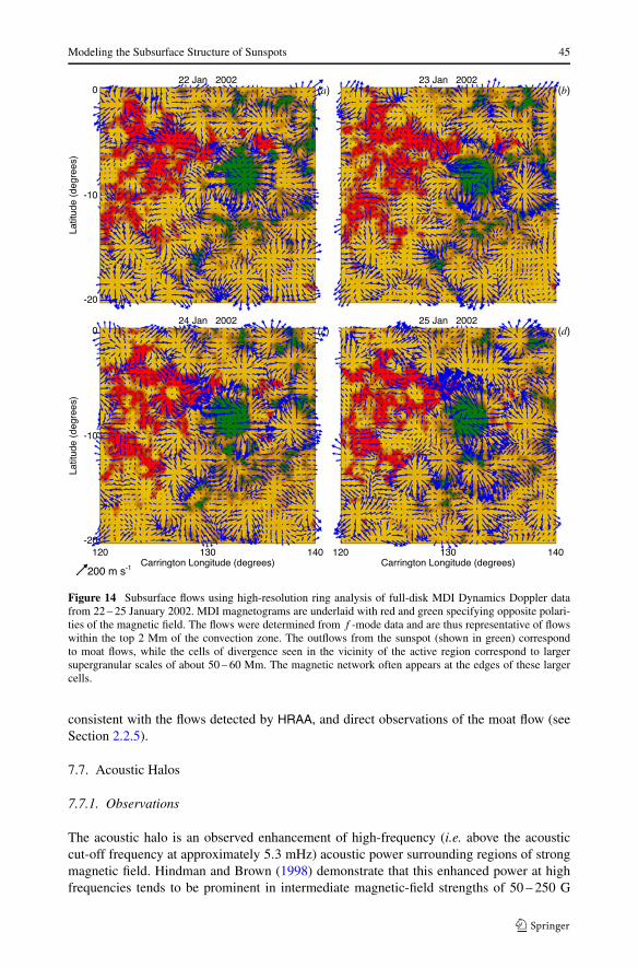
Modeling the Subsurface Structure of Sunspots 45
Figure 14 Subsurface flows using high-resolution ring analysis of full-disk MDI Dynamics Doppler datafrom 22 – 25 January 2002. MDI magnetograms are underlaid with red and green specifying opposite polari-ties of the magnetic field. The flows were determined from f -mode data and are thus representative of flowswithin the top 2 Mm of the convection zone. The outflows from the sunspot (shown in green) correspondto moat flows, while the cells of divergence seen in the vicinity of the active region correspond to largersupergranular scales of about 50 – 60 Mm. The magnetic network often appears at the edges of these largercells.
consistent with the flows detected by HRAA, and direct observations of the moat flow (seeSection 2.2.5).
7.7. Acoustic Halos
7.7.1. Observations
The acoustic halo is an observed enhancement of high-frequency (i.e. above the acousticcut-off frequency at approximately 5.3 mHz) acoustic power surrounding regions of strongmagnetic field. Hindman and Brown (1998) demonstrate that this enhanced power at highfrequencies tends to be prominent in intermediate magnetic-field strengths of 50 – 250 G
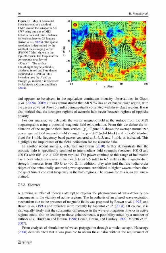
46 H. Moradi et al.
Figure 15 Map of horizontalflows (arrows) at a depth of1 Mm around the sunspot in AR9787 using one day of MDIfull-disk data and time – distancehelioseismology on 24 January(Gizon et al., 2009a). The spatialresolution is determined by thewidth of the averaging kernel(FWHM 7 Mm) shown in thetop-left corner. The longest arrowcorresponds to a flow of450 m s−1. The surfaceline-of-sight magnetic field isdisplayed in red and blue shades(saturated at ± 350 G). Thisinversion uses the f and p1through p4 modes; it is discussedby Jackiewicz, Gizon, and Birch(2008).
and appears to be absent in the equivalent continuum intensity observations. In Gizonet al. (2009a, 2009b) it was demonstrated that AR 9787 has an extensive plage region, withthe excess power at above 5.5 mHz being spatially correlated with these plage regions. It wasalso noticed that the strongest regions of acoustic halo occur between regions of oppositepolarity.
For our analysis, we calculate the vector magnetic field at the surface from the MDImagnetograms using a potential magnetic-field extrapolation. From this we define the in-clination of the magnetic field from vertical [γ ]. Figure 16 shows the average normalizedpower against total magnetic-field strength for γ < 45◦ (solid black) and γ > 45◦ (dashedblue) for 1-mHz frequency band passes centered at 3, 4, 5, and 6 mHz as indicated. Thishighlights the importance of the field inclination for the acoustic halo.
In another recent analysis, Schunker and Braun (2010) further demonstrate that theacoustic halo is specifically confined to intermediate field strengths (between 100 G and400 G) with 60◦ < γ < 120◦ from vertical. The power confined to this range of inclinationhas a peak which increases in frequency from 5.5 mHz to 6.5 mHz as the magnetic-fieldstrength increases from 100 G to 400 G. In addition, they also find that the radial-orderridges of the azimuthally summed power spectrum are shifted to higher wavenumbers thanthe quiet Sun at constant frequency in the halo regions. The reason for this is, as yet, unex-plained.
7.7.2. Theories
A growing number of theories attempt to explain the phenomenon of wave-velocity en-hancements in the vicinity of active regions. The hypothesis of an altered wave excitationmechanism due to the presence of magnetic fields was proposed by Brown et al. (1992) andBraun et al. (1992) and revisited more recently by Jacoutot et al. (2008). Of course, it isalso equally likely that the substantial differences in the wave-propagation physics in activeregions could also be leading to these enhancements, a possibility noted by a number ofauthors (e.g. Hindman and Brown, 1998; Donea, Braun, and Lindsey, 1999; Moretti et al.,2007).
From analyses of simulations of waves propagation through a model sunspot, Hanasoge(2008) demonstrated that it was possible to obtain these halos without the requirement of
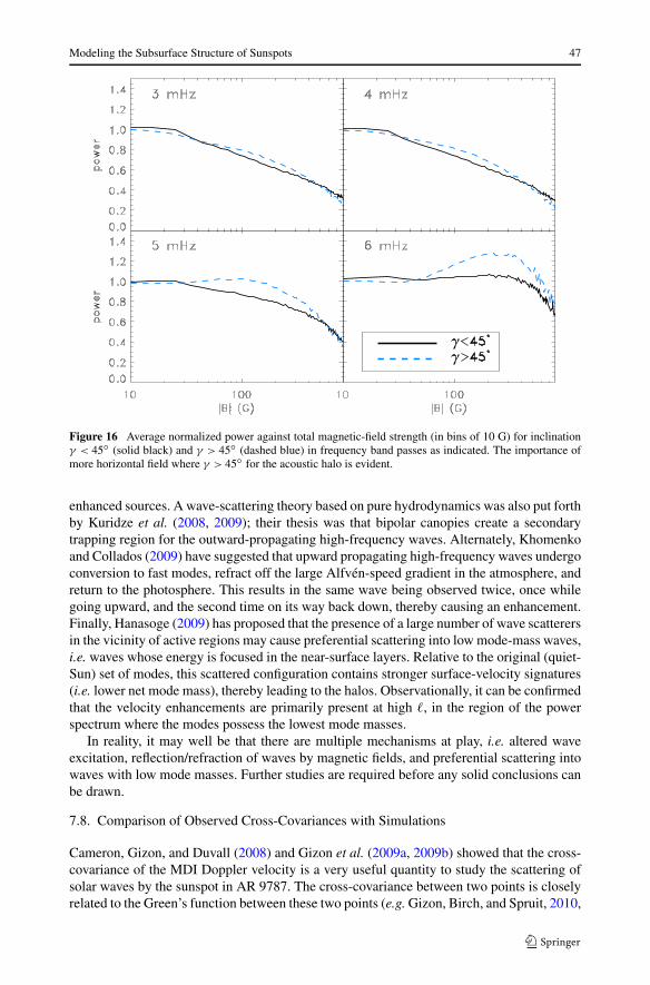
Modeling the Subsurface Structure of Sunspots 47
Figure 16 Average normalized power against total magnetic-field strength (in bins of 10 G) for inclinationγ < 45◦ (solid black) and γ > 45◦ (dashed blue) in frequency band passes as indicated. The importance ofmore horizontal field where γ > 45◦ for the acoustic halo is evident.
enhanced sources. A wave-scattering theory based on pure hydrodynamics was also put forthby Kuridze et al. (2008, 2009); their thesis was that bipolar canopies create a secondarytrapping region for the outward-propagating high-frequency waves. Alternately, Khomenkoand Collados (2009) have suggested that upward propagating high-frequency waves undergoconversion to fast modes, refract off the large Alfvén-speed gradient in the atmosphere, andreturn to the photosphere. This results in the same wave being observed twice, once whilegoing upward, and the second time on its way back down, thereby causing an enhancement.Finally, Hanasoge (2009) has proposed that the presence of a large number of wave scatterersin the vicinity of active regions may cause preferential scattering into low mode-mass waves,i.e. waves whose energy is focused in the near-surface layers. Relative to the original (quiet-Sun) set of modes, this scattered configuration contains stronger surface-velocity signatures(i.e. lower net mode mass), thereby leading to the halos. Observationally, it can be confirmedthat the velocity enhancements are primarily present at high �, in the region of the powerspectrum where the modes possess the lowest mode masses.
In reality, it may well be that there are multiple mechanisms at play, i.e. altered waveexcitation, reflection/refraction of waves by magnetic fields, and preferential scattering intowaves with low mode masses. Further studies are required before any solid conclusions canbe drawn.
7.8. Comparison of Observed Cross-Covariances with Simulations
Cameron, Gizon, and Duvall (2008) and Gizon et al. (2009a, 2009b) showed that the cross-covariance of the MDI Doppler velocity is a very useful quantity to study the scattering ofsolar waves by the sunspot in AR 9787. The cross-covariance between two points is closelyrelated to the Green’s function between these two points (e.g. Gizon, Birch, and Spruit, 2010,
48 H. Moradi et al.
and references therein). By extension, the cross-covariance between the signal averaged overa line and any other point can be used to study the interaction of plane-wave packets withthe sunspot.
The left panels in Figure 17 show such cross-covariances at particular values of thecorrelation time lag, after the wave packets have traversed the sunspot. While Gizonet al. (2009a, 2009b) had studied only f -mode wave packets, here we also show the ob-served cross-covariances for p1 and p2 wave packets. The wave packets are constructed us-ing standard ridge filters (wave power peaks near 3 mHz). The observed cross-covariancesshow that, in all cases, solar waves speed up through the sunspot and that their amplitudesare reduced relative to the quiet Sun. The stochastic noise in the observations is reduced byexploiting all available symmetries, including the near-cylindrical symmetry of the sunspot.
The cross-covariances also provide very strong observational constraints to test the va-lidity of sunspot models. Here we have used the SLiM code to test the semi-empirical modelof AR 9787 by Cameron et al. (2010) (see Section 4.3.1 and Figure 4) by propagating f , p1,and p2 wave packets through the sunspot model. The initial conditions of the simulations arechosen such that the vertical component of velocity in the simulation is directly comparablewith the cross-covariance function. As can be seen in Figure 17, the simulations reproducethe basic features of the observations. This indicates that the sunspot model has a seismicsignature that is close to the real sunspot, which is very encouraging.
8. Discussion and Perspective
8.1. Sunspot Structure: A Critical Assessment of Existing Models
Recent years have seen an increased interest in questions relating to the structure of sunspots,fueled by a fortunate coincidence of several factors. After decades of more gradual improve-ments, classical (visible light) observations have quickly improved in quality over the pastfew years. With the Swedish 1-m Solar Telescope, spatial resolution achieved has made ajump (with a resolution of 0.1′′ achieved regularly in the blue), while temporal coverage hasvastly improved through the long time sequences from the Hinode satellite. Secondly, helio-seismic observations have now approached the point where they can be turned into powerfuldiagnostics of spot structure, as discussed elsewhere in this article. Finally, and perhaps mostdramatically, the realism achieved by 3D radiative MHD simulations has now opened theperspective of a definitive physical interpretation of the phenomenology of sunspot struc-ture, including umbral dots, light bridges, penumbral filaments, the Evershed flow, the moatflow, and their relations to each other. It is likely that understanding will soon replace thehistorically evolved patchwork of mutually inconsistent views and physically dubious ad-hoc models. The following gives a brief perspective on these developments. For more detail,see the reviews in Scharmer (2009) and Nordlund and Scharmer (2010).
As discussed in Section 3, the structure of a sunspot as observed at the surface is kepttogether by forces deeper down. Assuming this anchoring at depth as given (but yet to beexplained), one can seek a physical interpretation of the surface structure observed in umbraeand penumbrae. At the observed field strengths, 1 – 3 kG, the magnetic field is strong enoughto suppress convection. This explains why spots are dark but it does not explain the particulartime-dependent fine structure observed.
In early observational work (e.g. Mamadazimov, 1972) the mix of long dark and brightfilaments has been interpreted as showing a magnetic field (dark, as in the umbra) on top ofthe normal photosphere (shining through in the bright filaments). This explained the general
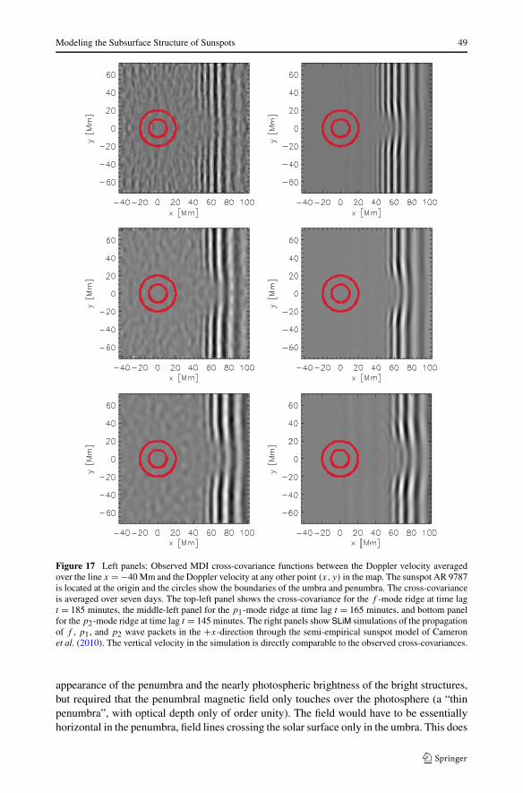
Modeling the Subsurface Structure of Sunspots 49
Figure 17 Left panels: Observed MDI cross-covariance functions between the Doppler velocity averagedover the line x = −40 Mm and the Doppler velocity at any other point (x, y) in the map. The sunspot AR 9787is located at the origin and the circles show the boundaries of the umbra and penumbra. The cross-covarianceis averaged over seven days. The top-left panel shows the cross-covariance for the f -mode ridge at time lagt = 185 minutes, the middle-left panel for the p1-mode ridge at time lag t = 165 minutes, and bottom panelfor the p2-mode ridge at time lag t = 145 minutes. The right panels show SLiM simulations of the propagationof f , p1, and p2 wave packets in the +x-direction through the semi-empirical sunspot model of Cameronet al. (2010). The vertical velocity in the simulation is directly comparable to the observed cross-covariances.
appearance of the penumbra and the nearly photospheric brightness of the bright structures,but required that the penumbral magnetic field only touches over the photosphere (a “thinpenumbra”, with optical depth only of order unity). The field would have to be essentiallyhorizontal in the penumbra, field lines crossing the solar surface only in the umbra. This does
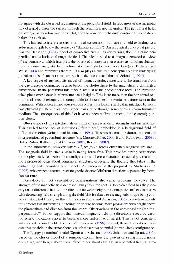
50 H. Moradi et al.
not agree with the observed inclination of the penumbral field. In fact, most of the magneticflux of a spot crosses the surface through the penumbra, not the umbra. The penumbral field,on average, is therefore not horizontal, and the observed field must continue to some depthbelow the surface.
This has led to interpretations in terms of convection in a magnetic field extending to asubstantial depth below the surface (a “thick penumbra”). An influential conceptual picturewas the Danielson (1961) model of convective “rolls”: an overturning flow in a plane per-pendicular to a horizontal magnetic field. This idea has led to a “magnetoconvection” viewof the penumbra, which interprets the observed filamentary structures as turbulent fluctua-tions in a mean magnetic field inclined at some angle to the solar surface (e.g. Tildesley andWeiss, 2004 and references therein). It also plays a role as a conceptual picture underlyingglobal models of sunspot structure, such as the one due to Jahn and Schmidt (1994).
A key aspect of any realistic model of magnetic surface structure is the transition fromthe gas-pressure dominated regime below the photosphere to the magnetically dominatedatmosphere. In the penumbra this takes place just at the photospheric level. The transitiontakes place over a couple of pressure scale heights. This is no more than the horizontal res-olution of most telescopes, and comparable to the smallest horizontal structures seen in thepenumbra. With photospheric observations one is thus looking at the thin interface betweentwo physically different regimes, rather than a slice through some quasi-uniform turbulentmedium. The consequences of this fact have not been realized in most of the currently pop-ular views.
Observations of this interface show a mix of magnetic-field strengths and inclinations.This has led to the idea of inclusions (“flux tubes”) embedded in a background field ofdifferent direction (Solanki and Montavon, 1993). This has become the dominant theme ininterpretations of penumbral structure (e.g. Martínez Pillet, 2000; Bellot Rubio et al., 2003b;Bellot Rubio, Balthasar, and Collados, 2004; Borrero, 2007).
In the atmosphere, however, where B2/8π P , forces other than magnetic are small.The magnetic field in such a case is nearly force free. This provides strong restrictionson the physically realizable field configurations. These constraints are actually violated inmost proposed ideas about penumbral structure, especially the floating flux tubes in theembedding and uncombed type models. An exception is the proposal by Martens et al.(1996), who propose a structure of magnetic sheets of different directions separated by force-free currents.
Force-free, but not current-free, configurations also cause problems, however. Thestrength of the magnetic field decreases away from the spot. A force-free field has the prop-erty that a difference in field-line direction between neighboring magnetic surfaces increaseswith decreasing field strength along the field (this is related to the magnetic torque being con-served along field lines; see the discussion in Spruit and Scharmer, 2006). Force-free modelsthus predict that differences in inclination should become more prominent with height abovethe photosphere and distance from the umbra. Observations in the chromosphere (the “su-perpenumbra”) do not support this. Instead, magnetic-field-line directions traced by chro-mospheric indicators appear to become more uniform with height. This is not consistentwith force-free models like those of Martens et al. (1996). Instead, these observations indi-cate that the field in the atmosphere is much closer to a potential (current-free) configuration.
The “gappy penumbra” model (Spruit and Scharmer, 2006; Scharmer and Spruit, 2006),based on the cluster model of a sunspot, explains how the pattern of strong irregularitiesdecreasing with height above the surface comes about naturally in a potential field, as a re-
Modeling the Subsurface Structure of Sunspots 51
sult of gaps between field lines created below the surface by overturning convection.1 Atthe same time this model addresses the long-standing heat-flow problem: the question ofhow the observed radiative energy flux is supplied to the penumbral surface. The low fieldstrength in the gaps allows convection to supply the heat flux emitted by the surface unim-peded by magnetic forces. Convection in magnetic rolls, on the other hand, does not solvethis problem, since a roll with the diameter of a penumbral filament does not contain enoughthermal energy to maintain the radiative flux over the life of a filament. However, the gappymodel has problems explaining the structure in the outer penumbra, where observationsshow a nearly horizontal field (also confirmed in the numerical simulations of Rempel et al.,2009b), and the presence of returning magnetic flux (Section 2.2.1).
Apart from the gappy model, a number of other physical models for the penumbral cur-rently exist. The model of Schlichenmaier, Jahn, and Schmidt (1998) (see also Schlichen-maier, 2009 and references therein), which has the virtue of substantial physical detail, pre-scribes that magnetic-flux tubes rising from below the surface carry heat as well as an out-ward flow, interpreted as the Evershed flow. It has problems reproducing the observed heatflux from the penumbra, however, and the postulated rising flux tubes have not been iden-tified in the numerical simulations. In the numerical simulations, both the heat flux and theEvershed flow are found to be driven by overturning convection, not in the form of magneticrolls or flux tubes, but in regions low field strength (Nordlund and Scharmer, 2010).
Another proposal appeals to the process of “turbulent flux-pumping” (Thomas et al.,2002; Weiss et al., 2004). In this process asymmetry between upflows and downflowsin stratified convection effectively transports horizontal magnetic-field lines downward.Penumbral structure is then ascribed to this process. The source of the penumbral structure issaid to be located outside the penumbra (Weiss et al., 2004). Alternatively, it has also beenimplied to be located in the penumbra itself (Tildesley and Weiss, 2004). The turbulent-pumping mechanism appears to offer a plausible mechanism for producing the returningmagnetic flux in the outer penumbra, as well as the apparent hysteresis observed in the tran-sition between a pore and a sunspot (Weiss et al., 2004). However, there are also objectionsto this model that are based on the fact that the action of convection on a magnetic field over-lying it, as in the outer penumbra, would be expected to have the opposite effect of turbu-lent pumping. Overturning convection would instead expel a magnetic field that is imposedfrom above, through the well-known process of convective expulsion (Zel’dovich, 1956;Weiss, 1966). The process is seen in action in numerical simulations of horizontal magneticfields overlying granulation by Steiner et al. (2008, 2009).
As the quality of observations continues to improve, realistic, 3D, radiative, numeri-cal MHD simulations of sunspots (Schüssler and Vögler, 2006; Heinemann et al., 2007;Scharmer, Nordlund, and Heinemann, 2008; Rempel, Schüssler, and Knölker, 2009a;Rempel et al., 2009b) show a remarkable level of agreement with these observations. Theagreement includes the properties of umbral dots, the inward-propagating bright filaments,the dark cores overlying them, the varying aspect of penumbral structure with viewing angle,the varying field strengths and direction in penumbral filaments, the dependence of these onheight, the moat flow, and the Evershed flow. We expect that more advanced simulations
1By “overturning” we mean here the convective pattern also observed in realistic simulations of stellar surfaceconvection (see the review by Scharmer, 2009 for more detail). As opposed to traditional views approximatingconvection as closed cells or “rolls”, almost nothing of the descending part of the flow returns to the surface,but it is replaced by upflows from larger depths. As opposed to the field-aligned rolls of the Danielson (1961)kind, this pattern maintains a low field strength in the gaps through the process of convective expulsion.While these gaps may not be exactly field free (as none of the convection zone is), they are regions where thehydrodynamic forces dominate over magnetic forces, i.e., the field is “below equipartition with convection”.
52 H. Moradi et al.
in the near future will further improve our understanding of penumbrae, in particular withregard to their outermost parts. With this level of agreement with observations, there is littledoubt that the simulations are reproducing the physics of sunspot structure as observed atthe surface.
Next to the treatment of the atmospheric magnetic field, the physics of radiation is ofequal importance for realism in numerical simulations. Cooling by radiation at the surfacedetermines the thermal structure of the penumbra and drives the observed flows. On theother hand, it also determines the detailed appearance of penumbral structure at the opticaldepth unity surface. Any physically meaningful comparison with observations thus requiresinclusion of radiation physics at a fairly well-developed level. The fact that the level of real-ism needed for a meaningful interpretation of solar-surface structure, magnetic or quiet, hasnow been achieved should be considered one of the most significant advance in theoreticalsolar physics of the past few decades.
8.2. The Starspot Connection
It is important to keep in mind that our Sun is not the only star that possesses spots. More-over, it is more than likely that all late-type stars with convective envelopes exhibit spots, or“starspots” (e.g. reviews by Berdyugina, 2005 and Strassmeier, 2009). Spotted stars consti-tute roughly 90% of all stars in the Milky Way, basically all GKM stars and a large fractionof F, and L and T dwarfs are spotted, representing a mass range from the brown dwarf limitup to the 2.4 M� of a G giant, and an age range from the pre-main sequence phase up tothe asymptotic giant branch. Stars with planets can also be affected by magnetic processesand their magnetic environment may even affect close-in planets and back-react onto thestar (see e.g. Shkolnik, Walker, and Bohlender, 2003; Catala et al., 2007; Kashyap, Drake,and Saar, 2008; Lanza, 2008). Therefore, we must understand sunspots first, before we canunderstand starspots.
Models of starspots do not exist yet but the mere size difference suggests that a scalingfrom a sunspot model is not appropriate (e.g. Solanki and Unruh, 2004). While sunspotstypically cover 10−4 to 10−5 of the solar surface and only during solar maximum reachabout 10−3, the record holder among other stars is still the one big starspot seen on the K0giant XX Tri in December 1997 (Strassmeier, 1999). Based on the star’s Hipparcos distanceof 197 pc, the spot’s area covers approximately 12×20 R2�, i.e. 22% of the star’s hemisphereor 10 000 times the area of the largest sunspot group. Clearly, its emergence, structure, anddecay must be addressed on a global scale. Figure 18 shows a Zeeman – Doppler image ofthe active spotted star II Pegasi (Carroll et al., 2007) combined with a numerical simulationof a non-axisymmetric dynamo. Although it is just a demonstration example, it nonethelesshighlights the expected global starspot – dynamo connection.
8.3. Conflicting Helioseismic Observations
A prevalent, largely phenomenological, approach to modeling the subsurface structureof sunspots has been to treat the regions of magnetism as perturbations to the back-ground wave speed. These types of models have been constructed using a variety of local-helioseismic procedures. A comparison of structural (wave-speed) inversions for AR 9787using both ring-diagram analysis and time – distance helioseismology with phase-speed fil-ters was presented by Gizon et al. (2009a, 2009b), and it is partially reproduced in Fig-ure 19.
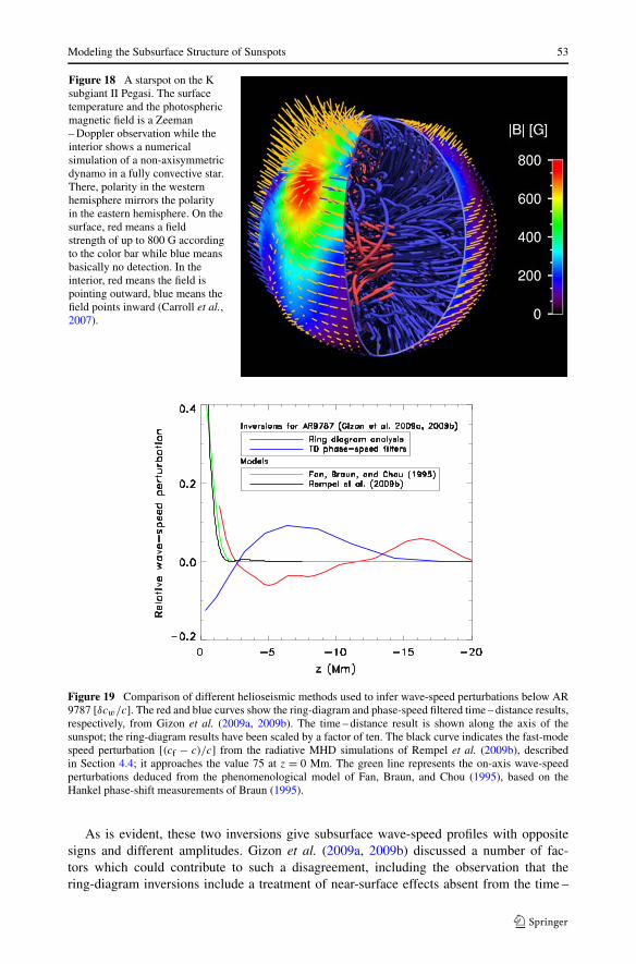
Modeling the Subsurface Structure of Sunspots 53
Figure 18 A starspot on the Ksubgiant II Pegasi. The surfacetemperature and the photosphericmagnetic field is a Zeeman– Doppler observation while theinterior shows a numericalsimulation of a non-axisymmetricdynamo in a fully convective star.There, polarity in the westernhemisphere mirrors the polarityin the eastern hemisphere. On thesurface, red means a fieldstrength of up to 800 G accordingto the color bar while blue meansbasically no detection. In theinterior, red means the field ispointing outward, blue means thefield points inward (Carroll et al.,2007).
Figure 19 Comparison of different helioseismic methods used to infer wave-speed perturbations below AR9787 [δcw/c]. The red and blue curves show the ring-diagram and phase-speed filtered time – distance results,respectively, from Gizon et al. (2009a, 2009b). The time – distance result is shown along the axis of thesunspot; the ring-diagram results have been scaled by a factor of ten. The black curve indicates the fast-modespeed perturbation [(cf − c)/c] from the radiative MHD simulations of Rempel et al. (2009b), describedin Section 4.4; it approaches the value 75 at z = 0 Mm. The green line represents the on-axis wave-speedperturbations deduced from the phenomenological model of Fan, Braun, and Chou (1995), based on theHankel phase-shift measurements of Braun (1995).
As is evident, these two inversions give subsurface wave-speed profiles with oppositesigns and different amplitudes. Gizon et al. (2009a, 2009b) discussed a number of fac-tors which could contribute to such a disagreement, including the observation that thering-diagram inversions include a treatment of near-surface effects absent from the time –
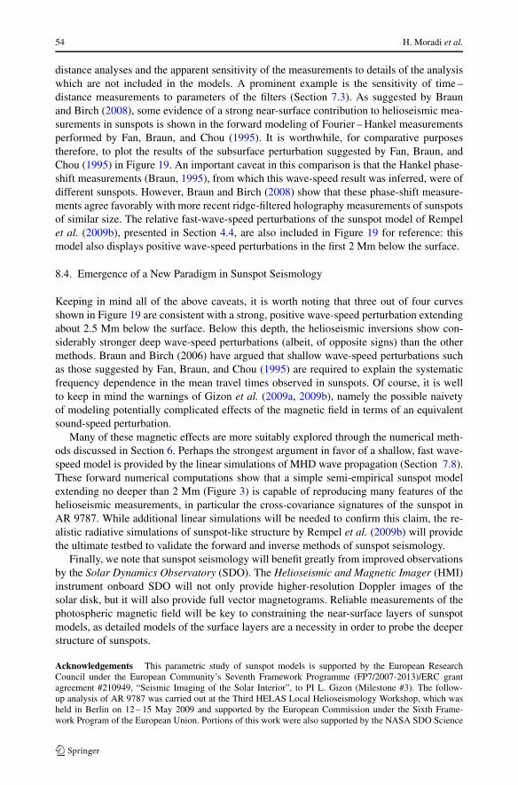
54 H. Moradi et al.
distance analyses and the apparent sensitivity of the measurements to details of the analysiswhich are not included in the models. A prominent example is the sensitivity of time –distance measurements to parameters of the filters (Section 7.3). As suggested by Braunand Birch (2008), some evidence of a strong near-surface contribution to helioseismic mea-surements in sunspots is shown in the forward modeling of Fourier – Hankel measurementsperformed by Fan, Braun, and Chou (1995). It is worthwhile, for comparative purposestherefore, to plot the results of the subsurface perturbation suggested by Fan, Braun, andChou (1995) in Figure 19. An important caveat in this comparison is that the Hankel phase-shift measurements (Braun, 1995), from which this wave-speed result was inferred, were ofdifferent sunspots. However, Braun and Birch (2008) show that these phase-shift measure-ments agree favorably with more recent ridge-filtered holography measurements of sunspotsof similar size. The relative fast-wave-speed perturbations of the sunspot model of Rempelet al. (2009b), presented in Section 4.4, are also included in Figure 19 for reference: thismodel also displays positive wave-speed perturbations in the first 2 Mm below the surface.
8.4. Emergence of a New Paradigm in Sunspot Seismology
Keeping in mind all of the above caveats, it is worth noting that three out of four curvesshown in Figure 19 are consistent with a strong, positive wave-speed perturbation extendingabout 2.5 Mm below the surface. Below this depth, the helioseismic inversions show con-siderably stronger deep wave-speed perturbations (albeit, of opposite signs) than the othermethods. Braun and Birch (2006) have argued that shallow wave-speed perturbations suchas those suggested by Fan, Braun, and Chou (1995) are required to explain the systematicfrequency dependence in the mean travel times observed in sunspots. Of course, it is wellto keep in mind the warnings of Gizon et al. (2009a, 2009b), namely the possible naivetyof modeling potentially complicated effects of the magnetic field in terms of an equivalentsound-speed perturbation.
Many of these magnetic effects are more suitably explored through the numerical meth-ods discussed in Section 6. Perhaps the strongest argument in favor of a shallow, fast wave-speed model is provided by the linear simulations of MHD wave propagation (Section 7.8).These forward numerical computations show that a simple semi-empirical sunspot modelextending no deeper than 2 Mm (Figure 3) is capable of reproducing many features of thehelioseismic measurements, in particular the cross-covariance signatures of the sunspot inAR 9787. While additional linear simulations will be needed to confirm this claim, the re-alistic radiative simulations of sunspot-like structure by Rempel et al. (2009b) will providethe ultimate testbed to validate the forward and inverse methods of sunspot seismology.
Finally, we note that sunspot seismology will benefit greatly from improved observationsby the Solar Dynamics Observatory (SDO). The Helioseismic and Magnetic Imager (HMI)instrument onboard SDO will not only provide higher-resolution Doppler images of thesolar disk, but it will also provide full vector magnetograms. Reliable measurements of thephotospheric magnetic field will be key to constraining the near-surface layers of sunspotmodels, as detailed models of the surface layers are a necessity in order to probe the deeperstructure of sunspots.
Acknowledgements This parametric study of sunspot models is supported by the European ResearchCouncil under the European Community’s Seventh Framework Programme (FP7/2007-2013)/ERC grantagreement #210949, “Seismic Imaging of the Solar Interior”, to PI L. Gizon (Milestone #3). The follow-up analysis of AR 9787 was carried out at the Third HELAS Local Helioseismology Workshop, which washeld in Berlin on 12 – 15 May 2009 and supported by the European Commission under the Sixth Frame-work Program of the European Union. Portions of this work were also supported by the NASA SDO Science
Modeling the Subsurface Structure of Sunspots 55
Center and Heliophysics Guest Investigator programs through contracts NNH09CE41C and NNG07EI51Cto NWRA under PI D.C. Braun. The authors would also like to acknowledge Kaori Nagashima and TakashiSekii for providing the Hinode observation used in Figure 1, and the anonymous referee for useful commentsthat helped improve the paper.
References
Albregtsen, F., Maltby, P.: 1978, Nature 274, 41. doi:10.1038/274041a0.Albregtsen, F., Maltby, P.: 1981, Solar Phys. 71, 269. doi:10.1007/BF00167551.Avrett, E.H.: 1981, In: Cram, L.E., Thomas, J.H. (eds.) The Physics of Sunspots, Sacramento Peak Observa-
tory, Sunspot, 235.Ayres, T.R.: 1996, In: Strassmeier, K.G., Linsky, J.L. (eds.) Stellar Surface Structure, IAU Sympos. 176,
Kluwer, Dordrecht, 371.Babcock, H.W.: 1963, Ann. Rev. Astron. Astrophys. 1, 41. doi:10.1146/annurev.aa.01.090163.000353.Backus, G.E., Gilbert, J.F.: 1967, Geophys. J. Int. 13, 247. doi:10.1111/j.1365-246X.1967.tb02159.x.Balthasar, H., Schmidt, W.: 1993, Astron. Astrophys. 279, 243.Balthasar, H., Wöhl, H.: 1983, Solar Phys. 88, 71. doi:10.1007/BF00196178.Balthasar, H., Schleicher, H., Bendlin, C., Volkmer, R.: 1996, Astron. Astrophys. 315, 603.Basu, S., Antia, H.M., Bogart, R.S.: 2004, Astrophys. J. 610, 1157. doi:10.1086/421843.Baumann, I., Schmitt, D., Schüssler, M., Solanki, S.K.: 2004, Astron. Astrophys. 426, 1075.
doi:10.1051/0004-6361:20048024.Beck, C.: 2008, Astron. Astrophys. 480, 825. doi:10.1051/0004-6361:20078409.Beckers, J.M., Schröter, E.H.: 1969, Solar Phys. 10, 384. doi:10.1007/BF00145526.Bellot Rubio, L.R.: 2003, In: Trujillo-Bueno, J., Sanchez Almeida, J. (eds.) Solar Polarization CS-307, As-
tron. Soc. Pacific, San Francisco, 301.Bellot Rubio, L.R., Balthasar, H., Collados, M.: 2004, Astron. Astrophys. 427, 319. doi:10.1051/0004-6361:
20041277.Bellot Rubio, L.R., Balthasar, H., Collados, M., Schlichenmaier, R.: 2003a, Astron. Astrophys. 403, L47.
doi:10.1051/0004-6361:20030576.Bellot Rubio, L.R., Balthasar, H., Collados, M., Schlichenmaier, R.: 2003b, Astron. Astrophys. 403, L47.
doi:10.1051/0004-6361:20030576.Berdyugina, S.V.: 2005, Living Rev. Solar Phys. 2, 8, http://solarphysics.livingreviews.org/Articles/lrsp-2005-8/.
Berenger, J.P.: 1994, J. Comput. Phys. 114, 185. doi:10.1006/jcph.1994.1159.Birch, A.C., Kosovichev, A.G., Duvall, T.L. Jr.: 2004, Astrophys. J. 608, 580. doi:10.1086/386361.Birch, A.C., Braun, D.C., Hanasoge, S.M., Cameron, R.: 2009, Solar Phys. 254, 17.
doi:10.1007/s11207-008-9282-9.Bogart, R.S., Basu, S., Rabello-Soares, M.C., Antia, H.M.: 2008, Solar Phys. 251, 439.
doi:10.1007/s11207-008-9213-9.Bogdan, T.J.: 1999, Astrophys. J. 512, 471. doi:10.1086/306749.Bogdan, T.J., Brown, T.M., Lites, B.W., Thomas, J.H.: 1993, Astrophys. J. 406, 723. doi:10.1086/172483.Borrero, J.M.: 2007, Astron. Astrophys. 471, 967. doi:10.1051/0004-6361:20066776.Borrero, J.M., Solanki, S.K., Bellot Rubio, L.R., Lagg, A., Mathew, S.K.: 2004, Astron. Astrophys. 422, 1093.
doi:10.1051/0004-6361:20041001.Borrero, J.M., Lagg, A., Solanki, S.K., Collados, M.: 2005, Astron. Astrophys. 436, 333.
doi:10.1051/0004-6361:20042553.Borrero, J.M., Solanki, S.K., Lagg, A., Socas-Navarro, H., Lites, B.: 2006, Astron. Astrophys. 450, 383.
doi:10.1051/0004-6361:20054378.Brants, J.J., Zwaan, C.: 1982, Solar Phys. 80, 251. doi:10.1007/BF00147972.Braun, D.C.: 1995, Astrophys. J. 451, 859. doi:10.1086/176272.Braun, D.C., Birch, A.C.: 2006, Astrophys. J. Lett. 647, L187. doi:10.1086/507450.Braun, D.C., Birch, A.C.: 2008, Solar Phys. 251, 267. doi:10.1007/s11207-008-9152-5.Braun, D.C., Lindsey, C.: 2000, Solar Phys. 192, 307.Braun, D.C., Duvall, T.L. Jr., Labonte, B.J.: 1987, Astrophys. J. Lett. 319, L27. doi:10.1086/184949.Braun, D.C., Duvall, T.L. Jr., Labonte, B.J.: 1988, Astrophys. J. 335, 1015. doi:10.1086/166988.Braun, D.C., Birch, A.C., Lindsey, C.: 2004, In: Danesy, D. (ed.) SOHO 14 Helio- and Asteroseismology:
Towards a Golden Future SP-559, ESA, Noordwijk, 337.Braun, D.C., Duvall, T.L. Jr., Labonte, B.J., Jefferies, S.M., Harvey, J.W., Pomerantz, M.A.: 1992, Astrophys.
J. Lett. 391, L113. doi:10.1086/186410.
56 H. Moradi et al.
Bray, R.J., Loughhead, R.E.: 1964, Sunspots, Chapman Hall, London.Brickhouse, N.S., Labonte, B.J.: 1988, Solar Phys. 115, 43. doi:10.1007/BF00146229.Brown, T.M., Bogdan, T.J., Lites, B.W., Thomas, J.H.: 1992, Astrophys. J. Lett. 394, L65.
doi:10.1086/186473.Caccin, B., Gomez, M.T., Severino, G.: 1993, Astron. Astrophys. 276, 219.Caligari, P., Moreno-Insertis, F., Schüssler, M.: 1995, Astrophys. J. 441, 886. doi:10.1086/175410.Caligari, P., Schüssler, M., Moreno-Insertis, F.: 1998, Astrophys. J. 502, 481. doi:10.1086/305875.Cally, P.S.: 1991, J. Comput. Phys. 93, 411. doi:10.1016/0021-9991(91)90192-N.Cally, P.S.: 2001, Astrophys. J. 548, 473. doi:10.1086/318675.Cally, P.S.: 2005, Mon. Not. Roy. Astron. Soc. 358, 353. doi:10.1111/j.1365-2966.2005.08742.x.Cally, P.S.: 2006, Phil. Trans. Roy. Soc. Lond. Ser. A 364, 333.Cally, P.S.: 2009a, Mon. Not. Roy. Astron. Soc. 395, 1309. doi:10.1111/j.1365-2966.2009.14708.x.Cally, P.S.: 2009b, Solar Phys. 254, 241. doi:10.1007/s11207-008-9290-9.Cally, P.S., Crouch, A.D., Braun, D.C.: 2003, Mon. Not. Roy. Astron. Soc. 346, 381. doi:10.1046/j.1365-
2966.2003.07019.x.Cameron, R., Gizon, L., Daiffallah, K.: 2007, Astron. Nachr. 328, 313. doi:10.1002/asna.200610736.Cameron, R., Gizon, L., Duvall, T.L. Jr.: 2008, Solar Phys. 251, 291.Cameron, R., Schunker, H., Gizon, L., Pietarila, A.: 2010, Solar Phys. doi:10.1007/a11207-010-9631-3.Carroll, T.A., Kopf, M., Ilyin, I., Strassmeier, K.G.: 2007, Astron. Nachr. 328, 1043. doi:10.1002/asna.
200710884.Catala, C., Donati, J.F., Shkolnik, E., Bohlender, D., Alecian, E.: 2007, Mon. Not. Roy. Astron. Soc. 374, L42.
doi:10.1111/j.1745-3933.2006.00261.x.Caunt, S.E., Korpi, M.J.: 2001, Astron. Astrophys. 369, 706. doi:10.1051/0004-6361:20010157.Chen, K.-R., Chou, D.-Y., TON Team: 1996, Astrophys. J. 465, 985. doi:10.1086/177484.Cheung, M.C.M., Schüssler, M., Moreno-Insertis, F.: 2007, Astron. Astrophys. 467, 703. doi:10.1051/
0004-6361:20077048.Chitre, S.M.: 1963, Mon. Not. Roy. Astron. Soc. 126, 431.Chitre, S.M., Shaviv, G.: 1967, Solar Phys. 2, 150. doi:10.1007/BF00155915.Chou, D.Y., Sun, M.T., Chang, H.K.: 2000, Astrophys. J. 532, 622. doi:10.1086/308571.Chou, D., Liang, Z., Yang, M., Zhao, H., Sun, M.: 2009, Astrophys. J. Lett. 696, L106.
doi:10.1088/0004-637X/696/1/L106.Christensen-Dalsgaard, J., Dappen, W., Ajukov, S.V., Anderson, E.R., Antia, H.M., Basu, S., Baturin, V.A.,
Berthomieu, G., Chaboyer, B., Chitre, S.M., Cox, A.N., Demarque, P., Donatowicz, J., Dziembowski,W.A., Gabriel, M., Gough, D.O., Guenther, D.B., Guzik, J.A., Harvey, J.W., Hill, F., Houdek, G., Igle-sias, C.A., Kosovichev, A.G., Leibacher, J.W., Morel, P., Proffitt, C.R., Provost, J., Reiter, J., Rhodes,E.J. Jr., Rogers, F.J., Roxburgh, I.W., Thompson, M.J., Ulrich, R.K.: 1996, Science 272, 1286.
Collados, M., Martínez Pillet, V., Ruiz Cobo, B., del Toro Iniesta, J.C., Vazquez, M.: 1994, Astron. Astrophys.291, 622.
Couvidat, S., Birch, A.C., Kosovichev, A.G., Zhao, J.: 2004, Astrophys. J. 607, 554. doi:10.1086/383342.Couvidat, S., Gizon, L., Birch, A.C., Larsen, R.M., Kosovichev, A.G.: 2005, Astrophys. J. Suppl. 158, 217.
doi:10.1086/430423.Cowling, T.G.: 1946, Mon. Not. Roy. Astron. Soc. 106, 218.Cowling, T.G.: 1953, In: Kuiper, G.P. (ed.) The Sun, University of Chicago, Chicago, 532.Cowling, T.G.: 1957, Magnetohydrodynamics, Interscience, New York.Cowling, T.G.: 1976, Magnetohydrodynamics, Adam Hilger, Bristol.Crouch, A.D., Cally, P.S., Charbonneau, P., Braun, D.C., Desjardins, M.: 2005, Mon. Not. Roy. Astron. Soc.
363, 1188. doi:10.1111/j.1365-2966.2005.09515.x.Danielson, R.E.: 1961, Astrophys. J. 134, 289. doi:10.1086/147159.Deinzer, W.: 1965, Astrophys. J. 141, 548. doi:10.1086/148144.del Toro Iniesta, J.C., Tarbell, T.D., Ruiz Cobo, B.: 1994, Astrophys. J. 436, 400. doi:10.1086/174914.Ding, M.D., Fang, C.: 1989, Astron. Astrophys. 225, 204.Donea, A.C., Braun, D.C., Lindsey, C.: 1999, Astrophys. J. Lett. 513, L143. doi:10.1086/311915.D’Silva, S., Choudhuri, A.R.: 1993, Astron. Astrophys. 272, 621.Duvall, T.L. Jr., Gizon, L.: 2000, Solar Phys. 192, 177.Duvall, T.L. Jr., Kosovichev, A.G., Scherrer, P.H., Bogart, R.S., Bush, R.I., De Forest, C., Hoeksema, J.T.,
Schou, J., Saba, J.L.R., Tarbell, T.D., Title, A.M., Wolfson, C.J., Milford, P.N.: 1997, Solar Phys. 170,63.
Duvall, T.L. Jr., D’Silva, S., Jefferies, S.M., Harvey, J.W., Schou, J.: 1996, Nature 379, 235.Fan, Y.: 2001, Astrophys. J. Lett. 554, L111. doi:10.1086/320935.Fan, Y., Braun, D.C., Chou, D.Y.: 1995, Astrophys. J. 451, 877.Fan, Y., Fisher, G.H., McClymont, A.N.: 1994, Astrophys. J. 436, 907. doi:10.1086/174967.
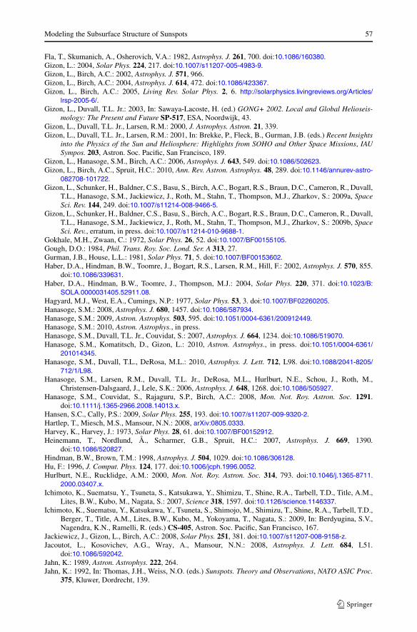
Modeling the Subsurface Structure of Sunspots 57
Fla, T., Skumanich, A., Osherovich, V.A.: 1982, Astrophys. J. 261, 700. doi:10.1086/160380.Gizon, L.: 2004, Solar Phys. 224, 217. doi:10.1007/s11207-005-4983-9.Gizon, L., Birch, A.C.: 2002, Astrophys. J. 571, 966.Gizon, L., Birch, A.C.: 2004, Astrophys. J. 614, 472. doi:10.1086/423367.Gizon, L., Birch, A.C.: 2005, Living Rev. Solar Phys. 2, 6. http://solarphysics.livingreviews.org/Articles/
lrsp-2005-6/.Gizon, L., Duvall, T.L. Jr.: 2003, In: Sawaya-Lacoste, H. (ed.) GONG+ 2002. Local and Global Helioseis-
mology: The Present and Future SP-517, ESA, Noordwijk, 43.Gizon, L., Duvall, T.L. Jr., Larsen, R.M.: 2000, J. Astrophys. Astron. 21, 339.Gizon, L., Duvall, T.L. Jr., Larsen, R.M.: 2001, In: Brekke, P., Fleck, B., Gurman, J.B. (eds.) Recent Insights
into the Physics of the Sun and Heliosphere: Highlights from SOHO and Other Space Missions, IAUSympos. 203, Astron. Soc. Pacific, San Francisco, 189.
Gizon, L., Hanasoge, S.M., Birch, A.C.: 2006, Astrophys. J. 643, 549. doi:10.1086/502623.Gizon, L., Birch, A.C., Spruit, H.C.: 2010, Ann. Rev. Astron. Astrophys. 48, 289. doi:10.1146/annurev-astro-
082708-101722.Gizon, L., Schunker, H., Baldner, C.S., Basu, S., Birch, A.C., Bogart, R.S., Braun, D.C., Cameron, R., Duvall,
T.L., Hanasoge, S.M., Jackiewicz, J., Roth, M., Stahn, T., Thompson, M.J., Zharkov, S.: 2009a, SpaceSci. Rev. 144, 249. doi:10.1007/s11214-008-9466-5.
Gizon, L., Schunker, H., Baldner, C.S., Basu, S., Birch, A.C., Bogart, R.S., Braun, D.C., Cameron, R., Duvall,T.L., Hanasoge, S.M., Jackiewicz, J., Roth, M., Stahn, T., Thompson, M.J., Zharkov, S.: 2009b, SpaceSci. Rev., erratum, in press. doi:10.1007/s11214-010-9688-1.
Gokhale, M.H., Zwaan, C.: 1972, Solar Phys. 26, 52. doi:10.1007/BF00155105.Gough, D.O.: 1984, Phil. Trans. Roy. Soc. Lond. Ser. A 313, 27.Gurman, J.B., House, L.L.: 1981, Solar Phys. 71, 5. doi:10.1007/BF00153602.Haber, D.A., Hindman, B.W., Toomre, J., Bogart, R.S., Larsen, R.M., Hill, F.: 2002, Astrophys. J. 570, 855.
doi:10.1086/339631.Haber, D.A., Hindman, B.W., Toomre, J., Thompson, M.J.: 2004, Solar Phys. 220, 371. doi:10.1023/B:
SOLA.0000031405.52911.08.Hagyard, M.J., West, E.A., Cumings, N.P.: 1977, Solar Phys. 53, 3. doi:10.1007/BF02260205.Hanasoge, S.M.: 2008, Astrophys. J. 680, 1457. doi:10.1086/587934.Hanasoge, S.M.: 2009, Astron. Astrophys. 503, 595. doi:10.1051/0004-6361/200912449.Hanasoge, S.M.: 2010, Astron. Astrophys., in press.Hanasoge, S.M., Duvall, T.L. Jr., Couvidat, S.: 2007, Astrophys. J. 664, 1234. doi:10.1086/519070.Hanasoge, S.M., Komatitsch, D., Gizon, L.: 2010, Astron. Astrophys., in press. doi:10.1051/0004-6361/
201014345.Hanasoge, S.M., Duvall, T.L., DeRosa, M.L.: 2010, Astrophys. J. Lett. 712, L98. doi:10.1088/2041-8205/
712/1/L98.Hanasoge, S.M., Larsen, R.M., Duvall, T.L. Jr., DeRosa, M.L., Hurlburt, N.E., Schou, J., Roth, M.,
Christensen-Dalsgaard, J., Lele, S.K.: 2006, Astrophys. J. 648, 1268. doi:10.1086/505927.Hanasoge, S.M., Couvidat, S., Rajaguru, S.P., Birch, A.C.: 2008, Mon. Not. Roy. Astron. Soc. 1291.
doi:10.1111/j.1365-2966.2008.14013.x.Hansen, S.C., Cally, P.S.: 2009, Solar Phys. 255, 193. doi:10.1007/s11207-009-9320-2.Hartlep, T., Miesch, M.S., Mansour, N.N.: 2008, arXiv:0805.0333.Harvey, K., Harvey, J.: 1973, Solar Phys. 28, 61. doi:10.1007/BF00152912.Heinemann, T., Nordlund, Å., Scharmer, G.B., Spruit, H.C.: 2007, Astrophys. J. 669, 1390.
doi:10.1086/520827.Hindman, B.W., Brown, T.M.: 1998, Astrophys. J. 504, 1029. doi:10.1086/306128.Hu, F.: 1996, J. Comput. Phys. 124, 177. doi:10.1006/jcph.1996.0052.Hurlburt, N.E., Rucklidge, A.M.: 2000, Mon. Not. Roy. Astron. Soc. 314, 793. doi:10.1046/j.1365-8711.
2000.03407.x.Ichimoto, K., Suematsu, Y., Tsuneta, S., Katsukawa, Y., Shimizu, T., Shine, R.A., Tarbell, T.D., Title, A.M.,
Lites, B.W., Kubo, M., Nagata, S.: 2007, Science 318, 1597. doi:10.1126/science.1146337.Ichimoto, K., Suematsu, Y., Katsukawa, Y., Tsuneta, S., Shimojo, M., Shimizu, T., Shine, R.A., Tarbell, T.D.,
Berger, T., Title, A.M., Lites, B.W., Kubo, M., Yokoyama, T., Nagata, S.: 2009, In: Berdyugina, S.V.,Nagendra, K.N., Ramelli, R. (eds.) CS-405, Astron. Soc. Pacific, San Francisco, 167.
Jackiewicz, J., Gizon, L., Birch, A.C.: 2008, Solar Phys. 251, 381. doi:10.1007/s11207-008-9158-z.Jacoutot, L., Kosovichev, A.G., Wray, A., Mansour, N.N.: 2008, Astrophys. J. Lett. 684, L51.
doi:10.1086/592042.Jahn, K.: 1989, Astron. Astrophys. 222, 264.Jahn, K.: 1992, In: Thomas, J.H., Weiss, N.O. (eds.) Sunspots. Theory and Observations, NATO ASIC Proc.
375, Kluwer, Dordrecht, 139.
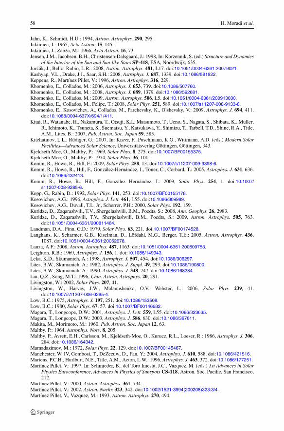
58 H. Moradi et al.
Jahn, K., Schmidt, H.U.: 1994, Astron. Astrophys. 290, 295.Jakimiec, J.: 1965, Acta Astron. 15, 145.Jakimiec, J., Zabza, M.: 1966, Acta Astron. 16, 73.Jensen, J.M., Jacobsen, B.H., Christensen-Dalsgaard, J.: 1998, In: Korzennik, S. (ed.) Structure and Dynamics
of the Interior of the Sun and Sun-like Stars SP-418, ESA, Noordwijk, 635.Jurcák, J., Bellot Rubio, L.R.: 2008, Astron. Astrophys. 481, L17. doi:10.1051/0004-6361:20079021.Kashyap, V.L., Drake, J.J., Saar, S.H.: 2008, Astrophys. J. 687, 1339. doi:10.1086/591922.Keppens, R., Martínez Pillet, V.: 1996, Astron. Astrophys. 316, 229.Khomenko, E., Collados, M.: 2006, Astrophys. J. 653, 739. doi:10.1086/507760.Khomenko, E., Collados, M.: 2008, Astrophys. J. 689, 1379. doi:10.1086/592681.Khomenko, E., Collados, M.: 2009, Astron. Astrophys. 506, L5. doi:10.1051/0004-6361/200913030.Khomenko, E., Collados, M., Felipe, T.: 2008, Solar Phys. 251, 589. doi:10.1007/s11207-008-9133-8.Khomenko, E., Kosovichev, A., Collados, M., Parchevsky, K., Olshevsky, V.: 2009, Astrophys. J. 694, 411.
doi:10.1088/0004-637X/694/1/411.Kitai, R., Watanabe, H., Nakamura, T., Otsuji, K.I., Matsumoto, T., Ueno, S., Nagata, S., Shibata, K., Muller,
R., Ichimoto, K., Tsuneta, S., Suematsu, Y., Katsukawa, Y., Shimizu, T., Tarbell, T.D., Shine, R.A., Title,A.M., Lites, B.: 2007, Pub. Astron. Soc. Japan 59, 585.
Kitchatinov, L.L., Rüdiger, G.: 2007, In: Kneer, F., Puschmann, K.G., Wittmann, A.D. (eds.) Modern SolarFacilities—Advanced Solar Science, Universitätsverlag Göttingen, Göttingen, 343.
Kjeldseth Moe, O., Maltby, P.: 1969, Solar Phys. 8, 275. doi:10.1007/BF00155375.Kjeldseth Moe, O., Maltby, P.: 1974, Solar Phys. 36, 101.Komm, R., Howe, R., Hill, F.: 2009, Solar Phys. 258, 13. doi:10.1007/s11207-009-9398-6.Komm, R., Howe, R., Hill, F., González-Hernández, I., Toner, C., Corbard, T.: 2005, Astrophys. J. 631, 636.
doi:10.1086/432413.Komm, R., Howe, R., Hill, F., González Hernández, I.: 2009, Solar Phys. 254, 1. doi:10.1007/
s11207-008-9285-6.Kopp, G., Rabin, D.: 1992, Solar Phys. 141, 253. doi:10.1007/BF00155178.Kosovichev, A.G.: 1996, Astrophys. J. Lett. 461, L55. doi:10.1086/309989.Kosovichev, A.G., Duvall, T.L. Jr., Scherrer, P.H.: 2000, Solar Phys. 192, 159.Kuridze, D., Zaqarashvili, T.V., Shergelashvili, B.M., Poedts, S.: 2008, Ann. Geophys. 26, 2983.Kuridze, D., Zaqarashvili, T.V., Shergelashvili, B.M., Poedts, S.: 2009, Astron. Astrophys. 505, 763.
doi:10.1051/0004-6361/200811484.Landman, D.A., Finn, G.D.: 1979, Solar Phys. 63, 221. doi:10.1007/BF00174528.Langhans, K., Scharmer, G.B., Kiselman, D., Löfdahl, M.G., Berger, T.E.: 2005, Astron. Astrophys. 436,
1087. doi:10.1051/0004-6361:20052678.Lanza, A.F.: 2008, Astron. Astrophys. 487, 1163. doi:10.1051/0004-6361:200809753.Leighton, R.B.: 1969, Astrophys. J. 156, 1. doi:10.1086/149943.Leka, K.D., Skumanich, A.: 1998, Astrophys. J. 507, 454. doi:10.1086/306297.Lites, B.W., Skumanich, A.: 1982, Astrophys. J. Suppl. 49, 293. doi:10.1086/190800.Lites, B.W., Skumanich, A.: 1990, Astrophys. J. 348, 747. doi:10.1086/168284.Liu, Q.Z., Song, M.T.: 1996, Chin. Astron. Astrophys. 20, 291.Livingston, W.: 2002, Solar Phys. 207, 41.Livingston, W., Harvey, J.W., Malanushenko, O.V., Webster, L.: 2006, Solar Phys. 239, 41.
doi:10.1007/s11207-006-0265-4.Low, B.C.: 1975, Astrophys. J. 197, 251. doi:10.1086/153508.Low, B.C.: 1980, Solar Phys. 67, 57. doi:10.1007/BF00146682.Magara, T., Longcope, D.W.: 2001, Astrophys. J. Lett. 559, L55. doi:10.1086/323635.Magara, T., Longcope, D.W.: 2003, Astrophys. J. 586, 630. doi:10.1086/367611.Makita, M., Morimoto, M.: 1960, Pub. Astron. Soc. Japan 12, 63.Maltby, P.: 1964, Astrophys. Norv. 8, 205.Maltby, P., Avrett, E.H., Carlsson, M., Kjeldseth-Moe, O., Kurucz, R.L., Loeser, R.: 1986, Astrophys. J. 306,
284. doi:10.1086/164342.Mamadazimov, M.: 1972, Solar Phys. 22, 129. doi:10.1007/BF00145467.Manchester, W. IV, Gombosi, T., DeZeeuw, D., Fan, Y.: 2004, Astrophys. J. 610, 588. doi:10.1086/421516.Martens, P.C.H., Hurlburt, N.E., Title, A.M., Acton, L.W.: 1996, Astrophys. J. 463, 372. doi:10.1086/177251.Martínez Pillet, V.: 1997, In: Schmieder, B., del Toro Iniesta, J.C., Vazquez, M. (eds.) 1st Advances in Solar
Physics Euroconference, Advances in Physics of Sunspots CS-118, Astron. Soc. Pacific, San Francisco,212.
Martínez Pillet, V.: 2000, Astron. Astrophys. 361, 734.Martínez Pillet, V.: 2002, Astron. Nachr. 323, 342. doi:10.1002/1521-3994(200208)323:3/4.Martínez Pillet, V., Vazquez, M.: 1993, Astron. Astrophys. 270, 494.
Modeling the Subsurface Structure of Sunspots 59
Mason, D., Komm, R., Hill, F., Howe, R., Haber, D., Hindman, B.W.: 2006, Astrophys. J. 645, 1543.doi:10.1086/503761.
Mathew, S.K., Lagg, A., Solanki, S.K., Collados, M., Borrero, J.M., Berdyugina, S., Krupp, N., Woch, J.,Frutiger, C.: 2003, Astron. Astrophys. 410, 695. doi:10.1051/0004-6361:20031282.
Mathew, S.K., Solanki, S.K., Lagg, A., Collados, M., Borrero, J.M., Berdyugina, S.: 2004, Astron. Astrophys.422, 693. doi:10.1051/0004-6361:20040136.
Mathew, S.K., Martínez Pillet, V., Solanki, S.K., Krivova, N.A.: 2007, Astron. Astrophys. 465, 291.doi:10.1051/0004-6361:20066356.
Mazzucconi, F., Coveri, C., Godoli, G.: 1990, Solar Phys. 125, 269. doi:10.1007/BF00158406.McIntosh, P.S.: 1981, In: Cram, L.E., Thomas, J.H. (eds.) The Physics of Sunspots, Sacramento Peak Obser-
vatory, Sunspot, 7.Meyer, F., Schmidt, H.U.: 1968, Mitt. Astron. Ges. Hamb. 25, 194.Montesinos, B., Thomas, J.H.: 1997, Nature 390, 485. doi:10.1038/37307.Moon, Y.J., Yun, H.S., Park, J.S.: 1998, Astrophys. J. 494, 851. doi:10.1086/305239.Moradi, H., Cally, P.S.: 2008, Solar Phys. 251, 309. doi:10.1007/s11207-008-9190-z.Moradi, H., Hanasoge, S.M.: 2010, In: Hasan, S.S., Rutten, R.J. (eds.) Magnetic Coupling between
the Interior and Atmosphere of the Sun, Astrophys. Space Sci. Proc., Springer, Berlin, 378.doi:10.1007/978-3-642-02859-5_35.
Moradi, H., Hanasoge, S.M., Cally, P.S.: 2009, Astrophys. J. Lett. 690, L72. doi:10.1088/0004-637X/690/1/L72.
Moretti, P.F., Jefferies, S.M., Armstrong, J.D., McIntosh, S.W.: 2007, Astron. Astrophys. 471, 961.doi:10.1051/0004-6361:20077247.
Nicolas, K.R., Bartoe, J.D.F., Brueckner, G.E., Kjeldseth-Moe, D.: 1981, In: Cram, L.E., Thomas, J.H. (eds.)The Physics of Sunspots, Sacramento Peak Observatory, Sunspot, 167.
Nordlund, Å., Scharmer, G.B.: 2010, In: Hasan, S.S., Rutten, R.J. (eds.) Magnetic Coupling betweenthe Interior and Atmosphere of the Sun, Astrophys. Space Sci. Proc., Springer, Berlin, 243.doi:10.1007/978-3-642-02859-5_18.
Norton, A.A., Gilman, P.A.: 2004, Astrophys. J. 603, 348. doi:10.1086/381362.Osherovich, V., Flaa, T.: 1983, Solar Phys. 88, 109. doi:10.1007/BF00196181.Osherovich, V.A.: 1982, Solar Phys. 77, 63. doi:10.1007/BF00156095.Osherovich, V.A., Garcia, H.A.: 1989, Astrophys. J. 336, 468. doi:10.1086/167025.Osherovich, V.A., Lawrence, J.K.: 1983, Solar Phys. 88, 117. doi:10.1007/BF00196182.Parchevsky, K.V., Kosovichev, A.G.: 2007, Astrophys. J. 666, 547. doi:10.1086/520108.Parchevsky, K.V., Kosovichev, A.G.: 2009, Astrophys. J. 694, 573. doi:10.1088/0004-637X/694/1/573.Parker, E.N.: 1975, Solar Phys. 40, 291. doi:10.1007/BF00162376.Parker, E.N.: 1979, Astrophys. J. 234, 333. doi:10.1086/157501.Penn, M.J., Livingston, W.: 2006, Astrophys. J. Lett. 649, L45. doi:10.1086/508345.Petrovay, K., Moreno-Insertis, F.: 1997, Astrophys. J. 485, 398. doi:10.1086/304404.Pizzo, V.J.: 1986, Astrophys. J. 302, 785. doi:10.1086/164041.Pizzo, V.J.: 1990, Astrophys. J. 365, 764. doi:10.1086/169530.Priest, E., Forbes, T.: 2000, Magnetic Reconnection, Cambridge University Press, Cambridge.Puschmann, K.G., Ruiz Cobo, B., Martínez Pillet, V.: 2008, arXiv:0810.2432.Rabello-Soares, M.C., Basu, S., Christensen-Dalsgaard, J.: 1999, Mon. Not. Roy. Astron. Soc. 309, 35.
doi:10.1046/j.1365-8711.1999.02785.x.Rajaguru, S.P., Birch, A.C., Duvall, T.L. Jr., Thompson, M.J., Zhao, J.: 2006, Astrophys. J. 646, 543.
doi:10.1086/504705.Rajaguru, S.P., Sankarasubramanian, K., Wachter, R., Scherrer, P.H.: 2007, Astrophys. J. Lett. 654, L175.
doi:10.1086/511266.Rast, M.P., Fox, P.A., Lin, H., Lites, B.W., Meisner, R.W., White, O.R.: 1999, Nature 401, 678.
doi:10.1038/44343.Rast, M.P., Meisner, R.W., Lites, B.W., Fox, P.A., White, O.R.: 2001, Astrophys. J. 557, 864.
doi:10.1086/321673.Rempel, M., Schüssler, M., Knölker, M.: 2009, Astrophys. J. 691, 640. doi:10.1088/0004-637X/691/1/640.Rempel, M., Schüssler, M., Cameron, R.H., Knölker, M.: 2009, Science 325, 171.
doi:10.1126/science.1173798.Riethmüller, T.L., Solanki, S.K., Zakharov, V., Gandorfer, A.: 2008, Astron. Astrophys. 492, 233.
doi:10.1051/0004-6361:200810701.Rimmele, T.: 2008, Astrophys. J. 672, 684. doi:10.1086/523702.Rimmele, T.R.: 1997, Astrophys. J. 490, 458. doi:10.1086/304863.Ringnes, T.S., Jensen, E.: 1960, Astrophys. Norv. 7, 99.Roden, A.J., Gedney, S.D.: 2000, Microwave Opt. Tech. Lett. 27, 334.
60 H. Moradi et al.
Rossbach, M., Schröter, E.H.: 1970, Solar Phys. 12, 95. doi:10.1007/BF02276568.Rouppe van der Voort, L.H.M.: 2002, Astron. Astrophys. 389, 1020. doi:10.1051/0004-6361:20020638.Rucklidge, A.M., Schmidt, H.U., Weiss, N.O.: 1995, Mon. Not. Roy. Astron. Soc. 273, 491.Ruiz Cobo, B., del Toro Iniesta, J.C.: 1992, Astrophys. J. 398, 375. doi:10.1086/171862.Sainz Dalda, A., Bellot Rubio, L.R.: 2008a, Astron. Astrophys. 481, L21. doi:10.1051/0004-6361:20079115.Sainz Dalda, A., Bellot Rubio, L.R.: 2008b, Astron. Astrophys. 481, L21. doi:10.1051/0004-6361:20079115.Scharmer, G.B.: 2009, Space Sci. Rev. 144, 229. doi:10.1007/s11214-008-9483-4.Scharmer, G.B., Spruit, H.C.: 2006, Astron. Astrophys. 460, 605. doi:10.1051/0004-6361:20066019.Scharmer, G.B., Nordlund, Å., Heinemann, T.: 2008, Astrophys. J. Lett. 677, L149. doi:10.1086/587982.Scharmer, G.B., Gudiksen, B.V., Kiselman, D., Löfdahl, M.G., Rouppe van der Voort, L.H.M.: 2002, Nature
420, 151.Schlichenmaier, R.: 2002, Astron. Nachr. 323, 303. doi:10.1002/1521-3994(200208)323:3/4.Schlichenmaier, R.: 2009, Space Sci. Rev. 144, 213. doi:10.1007/s11214-008-9465-6.Schlichenmaier, R., Collados, M.: 2002, Astron. Astrophys. 381, 668. doi:10.1051/0004-6361:20011459.Schlichenmaier, R., Schmidt, W.: 2000, Astron. Astrophys. 358, 1122.Schlichenmaier, R., Bellot Rubio, L.R., Tritschler, A.: 2004, Astron. Astrophys. 415, 731.
doi:10.1051/0004-6361:20034430.Schlichenmaier, R., Jahn, K., Schmidt, H.U.: 1998, Astron. Astrophys. 337, 897.Schlüter, A., Temesváry, S.: 1958, In: Lehnert, B. (ed.) Electromagnetic Phenomena in Cosmical Physics,
IAU Sympos. 6, Cambridge University Press, Cambridge, 263.Schmidt, H.U., Wegmann, R.: 1983, In: Brosowski, B., Martensen, E. (eds.) Dynamical Problems in Mathe-
matical Physics, Peter Lang, Bern, 137.Schmidt, W., Balthasar, H.: 1994, Astron. Astrophys. 283, 241.Schmidt, W., Hofmann, A., Balthasar, H., Tarbell, T.D., Frank, Z.A.: 1992, Astron. Astrophys. 264, L27.Schrijver, C.J.: 2001, Astrophys. J. 547, 475. doi:10.1086/318333.Schrijver, C.J., Title, A.M.: 1999, Solar Phys. 188, 331.Schunker, H., Braun, D.C. 2010, Solar Phys., doi:10.1007/s11207-010-9550-3.Schunker, H., Cally, P.S.: 2006, Mon. Not. Roy. Astron. Soc. 372, 551. doi:10.1111/j.1365-2966.
2006.10855.x.Schunker, H., Cameron, R., Gizon, L.: 2010, In: Elsworth, Y., Thompson, M. (eds.) Proceedings of the HELAS
Workshop NA3-4 “The Acoustic Solar Cycle”, Univ. Birmingham, 6–8 January 2009. arXiv:1002.1969.Schüssler, M.: 1984, Astron. Astrophys. 140, 453.Schüssler, M.: 1987, In: Durney, B.R., Sofia, S. (eds.) The Internal Solar Angular Velocity, Astrophys. Space
Sci. Lib. 137, Reidel, Dordrecht, 303.Schüssler, M., Rempel, M.: 2005, Astron. Astrophys. 441, 337. doi:10.1051/0004-6361:20052962.Schüssler, M., Vögler, A.: 2006, Astrophys. J. Lett. 641, L73. doi:10.1086/503772.Schüssler, M., Caligari, P., Ferriz-Mas, A., Moreno-Insertis, F.: 1994, Astron. Astrophys. 281, L69.Severino, G., Gomez, M.T., Caccin, B.: 1994, In: Rutten, R.J., Schrijver, C.J. (eds.) Solar Surface Magnetism,
Kluwer, Dordrecht, 169.Sheeley, N.R. Jr.: 1969, Solar Phys. 9, 347. doi:10.1007/BF02391657.Sheeley, N.R. Jr.: 1972, Solar Phys. 25, 98. doi:10.1007/BF00155747.Shelyag, S., Fedun, V., Erdélyi, R.: 2008, Astron. Astrophys. 486, 655. doi:10.1051/0004-6361:200809800.Shelyag, S., Zharkov, S., Fedun, V., Erdélyi, R., Thompson, M.J.: 2009, Astron. Astrophys. 501, 735.
doi:10.1051/0004-6361/200911709.Shkolnik, E., Walker, G.A.H., Bohlender, D.A.: 2003, Astrophys. J. 597, 1092. doi:10.1086/378583.Simon, G.W., Weiss, N.O.: 1970, Solar Phys. 13, 85. doi:10.1007/BF00963944.Simon, G.W., Weiss, N.O., Nye, A.H.: 1983, Solar Phys. 87, 65. doi:10.1007/BF00151161.Skumanich, A., Lites, B.W., Martínez Pillet, V.: 1994, In: Rutten, R.J., Schrijver, C.J. (eds.) Solar Surface
Magnetism, Kluwer, Dordrecht, 99.Sobotka, M.: 1997, In: Schmieder, B., del Toro Iniesta, J.C., Vazquez, M. (eds.) 1st Advances in Solar Physics
Euroconference. Advances in Physics of Sunspots CS-118, Astron. Soc. Pacific, San Francisco, 155.Sobotka, M.: 2002, In: Wilson, A. (ed.) Solar Variability: From Core to Outer Frontiers SP-506, ESA, No-
ordwijk, 381.Sobotka, M., Bonet, J.A., Vazquez, M.: 1993, Astrophys. J. 415, 832. doi:10.1086/173205.Socas-Navarro, H.: 2002, In: Sawaya-Lacoste, H. (ed.) SOLMAG 2002. Proceedings of the Magnetic Cou-
pling of the Solar Atmosphere Euroconference SP-505, ESA, Noordwijk, 45.Socas-Navarro, H.: 2005, Astrophys. J. Lett. 631, L167. doi:10.1086/497334.Socas-Navarro, H.: 2007, Astrophys. J. Suppl. 169, 439. doi:10.1086/510336.Socas-Navarro, H., Pillet, V.M., Sobotka, M., Vázquez, M.: 2004, Astrophys. J. 614, 448. doi:10.1086/
423487.
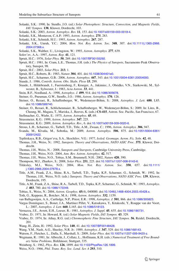
Modeling the Subsurface Structure of Sunspots 61
Solanki, S.K.: 1990, In: Stenflo, J.O. (ed.) Solar Photosphere: Structure, Convection, and Magnetic Fields,IAU Sympos. 138, Kluwer, Dordrecht, 103.
Solanki, S.K.: 2003, Astron. Astrophys. Rev. 11, 153. doi:10.1007/s00159-003-0018-4.Solanki, S.K., Montavon, C.A.P.: 1993, Astron. Astrophys. 275, 283.Solanki, S.K., Schmidt, H.U.: 1993, Astron. Astrophys. 267, 287.Solanki, S.K., Unruh, Y.C.: 2004, Mon. Not. Roy. Astron. Soc. 348, 307. doi:10.1111/j.1365-2966.
2004.07368.x.Solanki, S.K., Walther, U., Livingston, W.: 1993, Astron. Astrophys. 277, 639.Solov’ev, A.A.: 1997, Astron. Rep. 41, 121.Spruit, H.C.: 1976, Solar Phys. 50, 269. doi:10.1007/BF00155292.Spruit, H.C.: 1981, In: Cram, L.E., Thomas, J.H. (eds.) The Physics of Sunspots, Sacramento Peak Observa-
tory, Sunspot, 98.Spruit, H.C.: 2003, Solar Phys. 213, 1.Spruit, H.C., Roberts, B.: 1983, Nature 304, 401. doi:10.1038/304401a0.Spruit, H.C., Scharmer, G.B.: 2006, Astron. Astrophys. 447, 343. doi:10.1051/0004-6361:20054000.Staude, J.: 1986, Contrib. Astron. Obs. Skaln. Pleso 15, 299.Staude, J., Hildebrandt, J., Fuerstenberg, F., Krueger, A., Jakimiec, J., Obridko, V.N., Siarkowski, M., Syl-
wester, B., Sylwester, J.: 1983, Acta Astron. 33, 441.Stein, R.F., Nordlund, A.: 1998, Astrophys. J. 499, 914. doi:10.1086/305678.Steiner, O., Pneuman, G.W., Stenflo, J.O.: 1986, Astron. Astrophys. 170, 126.Steiner, O., Rezaei, R., Schaffenberger, W., Wedemeyer-Böhm, S.: 2008, Astrophys. J. Lett. 680, L85.
doi:10.1086/589740.Steiner, O., Rezaei, R., Schlichenmaier, R., Schaffenberger, W., Wedemeyer-Böhm, S.: 2009, In: Lites, B.,
Cheung, M., Magara, T., Mariska, J., Reeves, K. (eds.) CS-415, Astron. Soc. Pacific, San Francisco, 67.Stellmacher, G., Wiehr, E.: 1975, Astron. Astrophys. 45, 69.Strassmeier, K.G.: 1999, Astron. Astrophys. 347, 225.Strassmeier, K.G.: 2009, Astron. Astrophys. Rev., 6. doi:10.1007/s00159-009-0020-6.Strous, L.H., Scharmer, G., Tarbell, T.D., Title, A.M., Zwaan, C.: 1996, Astron. Astrophys. 306, 947.Svanda, M., Klvana, M., Sobotka, M.: 2009, Astron. Astrophys. 506, 875. doi:10.1051/0004-6361/
200912422.Teplitskaya, R.B., Grigor’eva, S.A., Skochilov, V.G.: 1977, Issled. Geomagn. Aeron. Fiz. Soln. 42, 48.Thomas, J.H., Weiss, N.: 1992, Sunspots. Theory and Observations, NATO ASIC Proc. 375, Kluwer, Dor-
drecht.Thomas, J.H., Weiss, N..: 2008, Sunspots and Starspots, Cambridge University Press, Cambridge.Thomas, J.H., Weiss, N.O.: 2004, Ann. Rev. Astron. Astrophys. 42, 517.Thomas, J.H., Weiss, N.O., Tobias, S.M., Brummell, N.H.: 2002, Nature 420, 390.Thompson, M.J., Zharkov, S.: 2008, Solar Phys. 251, 225. doi:10.1007/s11207-008-9143-6.Tildesley, M.J., Weiss, N.O.: 2004, Mon. Not. Roy. Astron. Soc. 350, 657. doi:10.1111/
j.1365-2966.2004.07678.x.Title, A.M., Frank, Z.A., Shine, R.A., Tarbell, T.D., Topka, K.P., Scharmer, G., Schmidt, W.: 1992, In:
Thomas, J.H., Weiss, N.O. (eds.) Sunspots. Theory and Observations, NATO ASIC Proc. 139, Kluwer,Dordrecht, 195.
Title, A.M., Frank, Z.A., Shine, R.A., Tarbell, T.D., Topka, K.P., Scharmer, G., Schmidt, W.: 1993, Astrophys.J. 403, 780. doi:10.1086/172249.
Tobias, S., Weiss, N.: 2004, Astron. Geophys. 45(4), 040000. doi:10.1046/j.1468-4004.2003.45428.x.Toth, G., Keppens, R., Botchev, M.A.: 1998, Astron. Astrophys. 332, 1159.van Ballegooijen, A.A., Cartledge, N.P., Priest, E.R.: 1998, Astrophys. J. 501, 866. doi:10.1086/305823.Vargas Domínguez, S., Bonet, J.A., Martínez Pillet, V., Katsukawa, Y., Kitakoshi, Y., Rouppe van der Voort,
L.: 2007, Astrophys. J. Lett. 660, L165. doi:10.1086/518123.Vernazza, J.E., Avrett, E.H., Loeser, R.: 1981, Astrophys. J. Suppl. 45, 635. doi:10.1086/190731.Vrabec, D.: 1971, In: Howard, R. (ed.) Solar Magnetic Fields, IAU Sympos. 43, 329.Vrabec, D.: 1974, In: Athay, R.G. (ed.) Chromospheric Fine Structure, IAU Sympos. 56, Reidel, Dordrecht,
201.Wang, H., Zirin, H.: 1992, Solar Phys. 140, 41. doi:10.1007/BF00148428.Wang, Y.M., Nash, A.G., Sheeley, N.R. Jr.: 1989, Astrophys. J. 347, 529. doi:10.1086/168143.Watson, F., Fletcher, L., Dalla, S., Marshall, S.: 2009, Solar Phys. doi:10.1007/s11207-009-9420-z.Wegmann, R.: 1981, In: Albrecht, J., Collatz, L., Hoffmann, K.H. (eds.) Numerical Treatment of Free Bound-
ary Value Problems, Birkhäuser, Stuttgart, 335.Weinberg, S.: 1962, Phys. Rev. 126, 1899. doi:10.1103/PhysRev.126.1899.Weiss, N.O.: 1966, Phil. Trans. Roy. Soc. Lond. Ser. A 293, 310.
62 H. Moradi et al.
Weiss, N.O., Thomas, J.H., Brummell, N.H., Tobias, S.M.: 2004, Astrophys. J. 600, 1073.doi:10.1086/380091.
Westendorp Plaza, C., del Toro Iniesta, J.C., Ruiz Cobo, B., Pillet, V.M.: 2001, Astrophys. J. 547, 1148.doi:10.1086/318377.
Yang, G., Xu, Y., Wang, H., Denker, C.: 2003, Astrophys. J. 597, 1190. doi:10.1086/377128.Yun, H.S.: 1970, Astrophys. J. 162, 975. doi:10.1086/150729.Yun, H.S.: 1971, Solar Phys. 16, 398. doi:10.1007/BF00162481.Yun, H.S., Beebe, H.A., Baggett, W.E.: 1984, Solar Phys. 92, 145. doi:10.1007/BF00157241.Yurchyshyn, V.B., Wang, H., Goode, P.R.: 2001, Astrophys. J. 550, 470. doi:10.1086/319717.Zel’dovich, Y.B.: 1956, Sov. J. Exp. Theor. Phys. 31, 154.Zhao, J., Kosovichev, A.G.: 2003, Astrophys. J. 591, 446.Zhao, J., Kosovichev, A.G.: 2004, Astrophys. J. 603, 776. doi:10.1086/381489.Zhao, J., Kosovichev, A.G., Duvall, T.L. Jr.: 2004, Astrophys. J. Lett. 607, L135. doi:10.1086/421974.Zwaan, C.: 1978, Solar Phys. 60, 213. doi:10.1007/BF00156523.Zwaan, C.: 1981, Space Sci. Rev. 28, 385. doi:10.1007/BF00212600.Zwaan, C.: 1992, In: Thomas, J.H., Weiss, N.O. (eds.) Sunspots. Theory and Observations, NATO ASIC Proc.
375, Kluwer, Dordrecht, 75.