monte carlo methods for web search
TRANSCRIPT

Monte Carlo Methods for Web Search

Monte Carlo Methods for Web Search
by Balazs Racz
Under the supervision of
Dr. Andras A. Benczur
Department of AlgebraBudapest University of Technology and Economics
Budapest
2009


Alulırott Racz Balazs kijelentem, hogy ezt a doktori ertekezest magam keszıtet-tem es abban csak a megadott forrasokat hasznaltam fel. Minden olyan reszt,amelyet szo szerint, vagy azonos tartalomban, de atfogalmazva mas forrasbolatvettem, egyertelmuen, a forras megadasaval megjeloltem.
Budapest, 2009. aprilis 14.
Racz Balazs
Az ertekezes bıralatai es a vedesrol keszult jegyzokonyv megtekintheto a Bu-dapesti Muszaki es Gazdasagtudomanyi Egyetem Termeszettudomanyi Kara-nak Dekani Hivatalaban.


Contents
1 Introduction 91.1 Overview . . . . . . . . . . . . . . . . . . . . . . . . . . . . . . . 101.2 How to Use this Thesis? . . . . . . . . . . . . . . . . . . . . . . 111.3 Introduction to the Datasets Used and the World Wide Web . . 111.4 The Scale of the Web . . . . . . . . . . . . . . . . . . . . . . . . 131.5 The Architecture of a Web Search Engine . . . . . . . . . . . . 151.6 The Computing Model . . . . . . . . . . . . . . . . . . . . . . . 161.7 Overview of Similarity Search Methods for the Web . . . . . . . 18
1.7.1 Text-based methods . . . . . . . . . . . . . . . . . . . . 191.7.2 Hybrid methods . . . . . . . . . . . . . . . . . . . . . . . 201.7.3 Simple graph-based methods . . . . . . . . . . . . . . . . 21
1.8 Introduction to Web Search Ranking . . . . . . . . . . . . . . . 221.8.1 The HITS ranking algorithm . . . . . . . . . . . . . . . . 231.8.2 The PageRank algorithm . . . . . . . . . . . . . . . . . . 24
1.9 Iterative Link-Based Similarity Functions . . . . . . . . . . . . . 251.9.1 The Companion similarity search algorithm . . . . . . . 251.9.2 The SimRank similarity function . . . . . . . . . . . . . 26
2 Personalized Web Search 292.1 Introduction . . . . . . . . . . . . . . . . . . . . . . . . . . . . . 29
2.1.1 Related Results . . . . . . . . . . . . . . . . . . . . . . . 302.1.2 Preliminaries . . . . . . . . . . . . . . . . . . . . . . . . 33
2.2 Personalized PageRank algorithm . . . . . . . . . . . . . . . . . 342.2.1 External memory indexing . . . . . . . . . . . . . . . . . 362.2.2 Distributed index computing . . . . . . . . . . . . . . . . 372.2.3 Query processing . . . . . . . . . . . . . . . . . . . . . . 39
2.3 How Many Fingerprints are Needed? . . . . . . . . . . . . . . . 402.4 Lower Bounds for PPR Database Size . . . . . . . . . . . . . . . 412.5 Experiments . . . . . . . . . . . . . . . . . . . . . . . . . . . . . 45
2.5.1 Comparison of ranking algorithms . . . . . . . . . . . . . 462.5.2 Results . . . . . . . . . . . . . . . . . . . . . . . . . . . . 47
2.6 Conclusions and Open Problems . . . . . . . . . . . . . . . . . . 49
7

8 CONTENTS
3 Similarity Search 513.1 Introduction . . . . . . . . . . . . . . . . . . . . . . . . . . . . . 51
3.1.1 Related Results . . . . . . . . . . . . . . . . . . . . . . . 533.1.2 Scalability Requirements . . . . . . . . . . . . . . . . . . 543.1.3 Preliminaries about SimRank . . . . . . . . . . . . . . . 54
3.2 Monte Carlo similarity search algorithms . . . . . . . . . . . . . 563.2.1 SimRank . . . . . . . . . . . . . . . . . . . . . . . . . . . 58
3.2.1.1 Fingerprint trees . . . . . . . . . . . . . . . . . 583.2.1.2 Fingerprint database and query processing . . . 603.2.1.3 Building the fingerprint database . . . . . . . . 61
3.2.2 PSimRank . . . . . . . . . . . . . . . . . . . . . . . . . . 623.2.2.1 Coupled random walks . . . . . . . . . . . . . . 623.2.2.2 Computing PSimRank . . . . . . . . . . . . . . 64
3.2.3 Updating the index database . . . . . . . . . . . . . . . . 643.3 Monte Carlo parallelization . . . . . . . . . . . . . . . . . . . . 663.4 Error of approximation . . . . . . . . . . . . . . . . . . . . . . . 673.5 Lower Bounds for the Similarity Database Size . . . . . . . . . . 693.6 Experiments . . . . . . . . . . . . . . . . . . . . . . . . . . . . . 72
3.6.1 Similarity Score Quality Measures . . . . . . . . . . . . . 733.6.2 Comparing the Quality under Various Parameter Settings 733.6.3 Time and memory requirement of fingerprint tree queries 753.6.4 Run-time Performance and Monte Carlo Parallelization . 76
3.7 Conclusion and open problems . . . . . . . . . . . . . . . . . . . 78
4 The Common Neighborhood Problem 814.1 Introduction . . . . . . . . . . . . . . . . . . . . . . . . . . . . . 814.2 Preliminaries . . . . . . . . . . . . . . . . . . . . . . . . . . . . 82
4.2.1 Data Stream Models . . . . . . . . . . . . . . . . . . . . 824.2.2 Common Neighborhoods . . . . . . . . . . . . . . . . . . 824.2.3 Communication Complexity . . . . . . . . . . . . . . . . 834.2.4 Previous Results on Streaming Graph Problems . . . . . 84
4.3 Single-pass data stream algorithms . . . . . . . . . . . . . . . . 854.4 O(1)-pass data stream algorithms . . . . . . . . . . . . . . . . . 894.5 Conclusion and open problems . . . . . . . . . . . . . . . . . . . 91
5 References 93

Chapter 1Introduction
One of the fastest growing sector of the software industry is that of the Inter-net companies, lead by the major search engines: Google, Yahoo and MSN.The importance of this field is even more emphasized by the plans of almostunprecedented magnitude that the European Union is pursuing to ease theirdependence on these US-based technological firms.
The scientific and technological difficulties of this field are dominated by themere scale: the web is estimated to contain tens to hundreds of billions of pages,with an exponential increase for over a decade and without showing any signsof that growth slowing down. At this scale, even the simplest mathematicalconstructs, such as a set of linear equations or a matrix inversion are turningout to be infeasible or practically unsolvable.
This thesis and the underlying publications provide solutions to certain ofthese scalability problems stemming from core web search engine research. Theactual problems and their abstract solutions are not ours; they were describedin earlier works of seminal authors of the field, generating considerable interest.Nevertheless, it was our work showing the first methods which could really scaleto the size of the web without serious limitations.
A particularly important aspect of our solutions is that they are not onlytheoretically applicable to the web, but also very practical: they follow fairlyclosely and naturally fit into the architecture of a web search engine; the algo-rithms are parallelizable or distributed; the computational model we assumedis the one that is present in all current major data centers; and the queryserving parts show characteristics very important for industrial applications,such as fault tolerance.
An important price we pay for these benefits is that out methods giveapproximate solutions to the abstract formulation. However, on one hand wehave strict bounds on the approximation quality, on the other hand we formallyprove that this is the only way to go: we give lower bounds on the resourceusage of any exact method, prohibiting their application on datasets on theWeb scale.
9
10 CHAPTER 1. INTRODUCTION
1.1 Overview
In the remaining of this chapter we define some terms, describe the architectureand introduce some methods common for the technical chapters. We will alsocover related results that are not strictly connected to either problems of theremaining chapters, but rather to the general methodology we use.
In Chapter 2 we consider the problem of personalized web search, alsocalled as personalized ranking. General web search has a static, global rankingfunction that the engine uses to sort the results according to some notion ofrelevance that depends on the query but not the user. However, relevance caneasily differ from user to user, e.g. a computer geek and a history teacher mayfind different sites authoritative and interesting for the same query. Person-alized web search allows users to specify their preference, and this preferenceparametrizes the ranking function. As PageRank is the most successful staticranking function, the personalized version, Personalized PageRank is of par-ticular interest. All earlier methods for computing personalized PageRankhad severe restrictions on what personalization they allowed. In our work weprovided the first Personalized PageRank algorithm allowing arbitrary person-alization and still scaling to the full Web. See Section 2.1 for further detailsand the respective chapter for our results.
In Chapter 3 we consider the problem of similarity search in massive graphssuch as the web. Similarity search is not only motivated by advanced datamining algorithms requiring easily computable similarity functions such asclustering algorithms, but also by the ‘Related pages’ functionality of websearch engines, where the user can query by example: supplying the URL ofa web page of interest, the search engine replies by good quality pages ona similar topic. Traditional similarity functions stemming in social networkanalysis such as co-citation express the similarity of two nodes in a graphby using only the neighbors of the nodes in question. However, consideringthe size and depth (e.g. average diameter) of the web graph, this is just asinadequate as using degree as a ranking function. We consider the similarityfunction proposed by Jeh and Widom, SimRank, which is a recursive definitionsimilar to that of PageRank. Our methods discussed in Chapter 3 provided thefirst algorithm that scaled beyond graphs of a few hundred thousand nodes.For further details and our results, see Section 3.1 and the respective chapter.
In the above chapters we follow the same outline: We first give approxima-tion algorithms for the problem, analyzing the approximation quality and con-vergence speed. Then we claim impossibility results about non-approximationapproaches, proving prohibitive space complexity. Finally we validate themethods using experiments on real Web datasets.
In the final chapter, Chapter 4 we pursue further impossibility results onsimilarity functions of massive graphs. We consider the decision problem: isthere a pair of vertices in a graph that share a common neighborhood of a par-ticular size? (This is equivalent to the existence of the complete bipartite graph

1.2. HOW TO USE THIS THESIS? 11
K2,c as a subgraph.) We are particularly interested in the space complexity ofthe problem in the data stream model: an algorithm A is allowed to read theset of edges of the graph sequentially, and after having one or constant manypasses, it has to output the answer to the decision problem. We lower boundthe temporary storage use of any such algorithm in the randomized computa-tion model. The relevance of this problem to web search is that an algorithmA for the decision problem can be emulated by a search engine. During thepreprocessing phase the search engine indexer can read the input a few times,producing an index database. Then the search engine query processor cananswer queries only the index database, and a proper sequence of queries givesus the answer to the decision problem. Therefore any lower bound we prove onthe decision problem applies either to the temporary storage requirements ofthe indexer, the query engine, or the index database size. A prohibitive (say,quadratic in the input size) lower bound makes it impossible to build a queryengine that can feasibly serve similarity queries up to the required precision.
1.2 How to Use this Thesis?
If you are interested in a thorough introduction and motivation for the topicscovered, read Chapter 1 up to this section, and Section 1 of each chapter youare interested in.
To get a general notion of the results, read the Abstract and Chapter 1 upto this section, skim through the first section and read the summary at theend of each chapter.
If you are interested in only one area, you can read any individual chapterin itself – this has been one of the main editing concepts behind this thesis. Youwill be referred back to the methodology sections of the Introduction whererequired.
To get pointers to related results, read Sections 2.1.1, 3.1.1, 4.1 and 4.2.4.Each chapter contains bibliographical notes, which detail the original pub-
lishing times and places of the results presented in that chapter, and, in ac-cordance with the authorship declaration, indication of authorship of eachindividual result presented in the chapter in case there were multiple authors.For the sake of completeness and readability we present all results includingthose that are attributed to co-authors of the original papers.
1.3 Introduction to the Datasets Used and the
World Wide Web
The main source of information that web search engines use is naturally theWorld Wide Web. There are several other datasets involved for example in thecomputation of quality signals such as manual ratings and collections, implicitor explicit feedback from users such as click logs [76], etc. which are mostly

12 CHAPTER 1. INTRODUCTION
unrelated to this thesis, except that we use data from the Open DirectoryProject to evaluate the quality of our similarity scores (See Section 3.6.1).
The World Wide Web is a distributed database, where certain computersconnected to the Internet are serving requests initiated by clients for contenthosted on those servers. The servers running a software conforming to one ofthe few retrieval protocols are called web servers. Clients trying to access aparticular content first determine which server is responsible for that content,and then connect to that server directly to fetch the data. The owner of thecontent is responsible for running the web servers and for registering in thedistributed database used for mapping of the resource locators to the actualservers.
Documents on the web are identified by Universal Resource Locator strings(in short URLs) such as http://www.ilab.sztaki.hu/~bracz/index.html. Inthis string http specifies the protocol to use for retrieving the data, www.ilab.sztaki.hu is the key using which the client computer looks up the serveraddress in the Domain Name System database, and /~bracz/index.html isthe identifier of the requested file on that particular server.
The vast majority of documents on the web use different versions of theHypertext Markup Language (HTML) format. This is a rich document for-mat used to describe formatted text with embedded media objects and cross-references between different portions of the web. The HTML files are viewed onthe user’s computer using a special software called web browser, which providesthe entire user experience, from fetching the URL contents, any embedded me-dia objects, formatting them to the screen, and providing navigational features.One of the most important navigational features are hyperlinks, which consistof a visual element (typically a piece of text, an image or a section of an image)that is active in the sense that the user can activate that element accordingto the input method used to communicate with the browser. With the mosttypical input method being a mouse or similar pointing device, the activationaction is usually a click on the visual element. When activated, the hyperlinkinstructs the web browser to load and display another URL to the user. Usingthese cross-referencing links the user can navigate between different pages ordifferent properties on the web, forming a smooth user experience of informa-tion consumption or free-time activity. In the rest of this thesis we may referto these hyperlinks as links.
One of the major challenge in the usability of the web is the vastly dis-tributed manner it is built. Server owners can decide by themselves whatcontent to publish, and the only way of reaching that content is to either knowthe exact URL under which it is published, or to accidentally find a link to it.Given that there are tens to hundreds of billions of pages and URLs, findinga particular piece of information is quite hopeless without services specificallydesigned to facilitate this. In the early years of the web these services weremostly hand-edited collections of links to web pages, also called directories.Later the significance of directories diminished in favor of web search engines,

1.4. THE SCALE OF THE WEB 13
which allow users to find relevant content on the web by phrasing a searchquery. The search engine then matches the search query against the entireweb, and returns the results to the user.
The information access method based on keyword searches in web searchengines presents a dual problem. On one hand, the user has to formulate aquery that is general enough so that the web page she is looking for matchesit, but specific enough so that there won’t be a huge amount of matches thatare unrelated and irrelevant to her. Restricting the URLs to check for theexpected content from 10 billion to one million or even a thousand is a bigstep, but still does not satisfy the user, as looking through hundreds of pagesto find the relevant content is not something web users are happy to do. So thesecond problem is for the search engine developers: given the current size ofthe web, any general query will match millions of documents. Given this hugeamount of matches, the search engine has to present them in such an order,that the one the user wishes to look at is among the topmost few. Of coursethis is an extremely underspecified problem (what is the intention of the userwhen she phrases a particular keyword query, and what webpages are the mostcorresponding to those intentions), and accordingly, the most successful websearch engines have been fine-tuning their ranking algorithms for several yearsor even a decade. For an introduction to search engine ranking, see Section 1.8.
1.4 The Scale of the Web
Any algorithm or service aiming to process the entire web is facing a significantchallenge stemming from the mere size of the web. In this section we try toquantify this size.
Due to the distributed and decentralized nature of the web, it is not easyto answer even the simplest questions about it such as
‘How many webpages are there in the World Wide Web?’
‘How many hyperlinks are there in the World Wide Web?’
To be more precise, these questions are pretty easy to answer, but theanswer quickly reveals that the questions are not formulated well enough sothat the answer would matter.
It is easy to see that the number of web pages and hyperlinks on the web isinfinite. Many web sites are exposing a human-readable form of a structureddatabase, where the HTML representation is generated by the serving machineusing arguments retrieved from the URL and the underlying database. Manyof these serving programs can accept arguments from an infinite domain andthus generate an infinite number of different pages.
An easy example is a calendar application, that displays some events in acertain time period, say a month. The page would typically have a link ‘nextmonth’ that will lead to a different page, containing the event list of the next

14 CHAPTER 1. INTRODUCTION
month. Following the ’next month’ links one will find an infinite sequence ofdifferent pages.
It is just as easy to see that such an infinite sequence does not contain aninfinite amount of useful pages, since the underlying database of information isfinite. In some other cases (for example a calculator that evaluates the formulathat the user inputs) it is the query page that is useful, not the individualresults of the individual queries.
Therefore we should rephrase the question as
‘How many useful webpages are there in the World Wide Web?’
and immediately conclude that we cannot give an exact answer due to themathematically uninterpretable condition useful.
Instead, we could turn to a slightly more practical matter, for example thequestion
‘How many webpages does the search engine X process?’
Unfortunately there is fairly little public information that would help usanswer this question. The major search engines (Google, Yahoo, MSN) donot publish this number. The recently launched web search startup Cuil [33]claims to be the world’s biggest web search engine with having crawled 186billion pages and serving 124 billion pages ([34], data as of January 2009) in itsindex. Unfortunately they don’t provide any reference or proof to their claimsabout the comparison to other search engines.
We can choose to rely on independent studies that try to estimate index sizeof search engines while treating them as blackboxes. A highly cited such study[61] has shown that the union of the major search engines’ index exceeds 11.5billion pages. The study was conducted in 2004, thus this number is severelyoutdated. A continuously updated study is published on [36], where (as ofJanuary 2009) multiple total size estimates are reported (e.g. 26 billion and63 billion).
The general problem with blackbox-based index size estimates is that theytypically need uniform sampling from within the blackbox, or relying on thestatistics reported for individual queries about the number of results. Both ofthese methods usually require a collection of terms to be supplied to the searchengine. Creating such collections from web-based datasets typically introducesome skew in the languages covered (e.g. [10] admits that the term collectiononly covers English). Furthermore, the statistics about the total number ofmatches for a query are approximations that can be seriously unreliable: Forexample in the case of a tiered index (for an introduction see [104]) it is quitepossible that the larger but more expensive index tiers are not consulted forsearches where earlier tiers return results of proper quality.
There is a general lack of recent research in the area since the search tech-nology has long since been focusing on the relevancy of results rather than

1.5. THE ARCHITECTURE OF A WEB SEARCH ENGINE 15
increasing index size: it is meaningless to return 2 million results to the userinstead of 1 million when the user practically never looks beyond the first ten.
We can conclude, that any algorithm not able to process over 10B pageswith reasonable machine resources is not acceptable for current leading searchengines.
1.5 The Architecture of a Web Search Engine
Here we provide a bird’s eye view of how search engines having (or at least aim-ing at having) entire web repositories work. Although the actual algorithmicand technical details are well-guarded secrets of the major search companies(Google, Yahoo and MSN), the outside frame of their architecture is commonlyunderstood to be the same.
Web search engines are centralized from the data store point of view. Theydownload all the content that is searchable and maintain a local copy at thedata center of the search engine. The process of downloading all available webcontent is called crawling, where an automated process follows every hyperlinkon pages visited so far and downloads their target pages, thereby extractingfurther hyperlinks, and so on. There are intricate details and non-trivial sci-entific and technological issues on several parts here [15, 85] which we omitas not being relevant to our subject matter such as the actual managementof the URLs waiting for download, parallelizing the crawling process to hun-dreds of machines, parallelizing hundreds of download threads on each of thosemachines, deciding whether and when to re-download an already seen page tolook for possible changes, etc.
The output of the crawling phase are two datasets: the first one containsall the HTML source of the web pages downloaded, while the second one (alsoobtainable from the first) is the web graph, where each web page is a vertex,and a hyperlink on page v pointing to page w is represented by a v → w arc.
These two datasets are fundamentally different, pose different problems andrequire a completely different class of algorithms to process even if the samequestion has to be solved such as similarity search based on textual data vs.similarity search in massive graphs [5]. The focus of our studies are algorithmsand problems formulated over the web graph.
As the crawler progresses by downloading newly appeared pages or refresh-ing existing pages [26], these datasets are constantly changing. Algorithms forefficiently incorporating these changes into the search engine’s current state(instead of re-computing the state from scratch for every little change) arevery important and could by themselves easily fill an entire monograph. Inmost of our studies here we assume to have a snapshot of these datasets, whilewe consider the incremental update problem of our similarity search solutionsin Section 3.2.3.
In a search engine these datasets are preprocessed to form the index data-base [108, 6]. This database by definition contains everything required to

16 CHAPTER 1. INTRODUCTION
compute the results to a query. The index is typically not a database as inthe traditional RDBMS sense, but rather a set of highly optimized specializedcomplex data structures to allow sub-second evaluation of user queries. Fur-thermore, a very important property is that the index is distributed : with itssize being measured in tens of terabytes, and query load totaling thousandsof queries per second, the only feasible supercomputing architecture for thisproblem is to employ a large number of parallelly operating cheap, small tomedium sized machines for storing the index database and serving the queries.
This architecture is depicted on Figure 1.1.
Compute quality signals
Process web graph
Process HTML of web pages
... Indexer
Preprocessing pipelineRepository
Crawler
Index
Serv
ing
wor
kers
Backendmixer
Frontend
queries
Internet
crawlerworkers
firewall
Crawl manager
Figure 1.1: Architecture of a web search engine from a bird’s eye view
1.6 The Computing Model
In this section we introduce the computing model and environment behind atypical web search engine.
When it comes to computing problems on the scale of the Web, even thebest algorithmic solution is going to use supercomputing resources: the sim-plest task of just reading and parsing the input dataset needs thousands ofhours of CPU and disk transfer time.
When it comes to supercomputing, there are in general two approaches:one is to install larger and more powerful computers, the other is to install a

1.6. THE COMPUTING MODEL 17
large amount of computers. As typically a computer of twice the capacity costsmore than twice more, it is easy to see that scaling to very high computingcapacity is the most cost effective if we employ a large multitude of small tomedium sized computers[20]. This choice was made by Google as detailed in[13].
Reducing the cost for a given computing capacity has always been a highpriority for the major web search engines. The exact methods used are well-guarded trade secrets, but there is a rack of a Google datacenter from 1999on display in the Computer History Museum in Mountain View, California.It is a big mess: the outer frame looks like a trolley in a cafeteria that holdsthe returned trays of dirty dishes, the computers in there have no case andthere are no rigid shelves: bare motherboards are bridging from side to sidein the frame. These motherboards are slightly bent from the weight the PCBis supporting. Commodity motherboards, CPUs and disks fill the entire rack,with two or four motherboards back-to-back on the same shelf. The only neatelement in the setup is the HP switch installed on the top of the rack.
According to this, the primary model used for designing algorithms weintend to run on the web is high level of parallelization[21, 95, 96]. The inputdataset has to be split into chunks, and we shall be able to distribute thesechunks of work to different machines, each of the capacity of a commodityPC. These machines are interconnected with some form of network, which istypically also commodity Ethernet. The machines can exchange informationover this network, but this exchange is also considered to be a cost, whereas anydata available in the local machine is much better accessible. Furthermore, theaccess to disk is also severely restricted: doing one disk seek (8 ms) sequentiallyfor every web page in a 10 billion-page crawl on a single disk would take 2.5years (assuming the disk drive can withstand such a utilization), so we wouldneed about 1000 drives to complete the computation within a day. On the otherhand, the same 1000-disk farm can transfer 1.73 PetaBytes of data to the CPUin a day when sequentially reading files at 20 MB/sec speed. Furthermore, if weconsider the 1000 machine cluster to contain 4 GB of RAM in each computer,then we can distribute 4 TB of data among the cluster such that each computerloads a chunk of it in memory, and is able to serve random lookup queries innanoseconds instead of in 8 ms from disk as in the previous example.
With these constraints originating from the underlying computing architec-ture, and the immense scale of the Web come the following strict requirementson the algorithms we are about to develop:
• Precomputation: The method consists of two parts: an off-line pre-computation phase, which is allowed to run for about a day to precom-pute an index database, and an on-line query serving part, which canaccess only the index database, and needs to answer a query within afew hundred milliseconds.
• Time: The index database is precomputed within the time of a sorting

18 CHAPTER 1. INTRODUCTION
operation, up to a constant factor. To serve a query the index databasecan only be accessed a constant number of times.
• Memory: The algorithms run in external memory : the available mainmemory is constant, so it can be arbitrarily smaller than the size ofthe web graph. In some cases we will consider semi-external-memoryalgorithms [91] with linear memory requirement in the number of verticesin the web graph, with a small constant factor.
• Parallelization: Both precomputation and query part can be imple-mented to utilize the computing power and storage capacity of thousandsof servers interconnected with a fast local network.
1.7 Overview of Similarity Search Methods for
the Web
The similarity ranking functions can be grouped into three main classes:
Text-based methods treat the web as a set of plain (or formatted) textdocuments, using classic methods of text database information retrieval[108].
Hybrid methods combine the text of a document with the text of the hyper-links pointing to that document (the so-called anchor text) or even withthe text surrounding the anchors. The intuition behind these methods isthat the anchor text is typically a very good summary of the documentpointed [3], since the reader of the linking page must decide whether toclick on the hyperlink purely based on the anchor text and its surround-ing context. This intuition was proven by various experiments [44].
The main problem with text-based and hybrid methods is that the webas a textual database is very heterogeneous, at the very least because ofthe many languages it is written in.
Graph-based methods restrict themselves exclusively on looking at the graphof the hyperlinks to decide the similarity of pages. These avoid the prob-lem of heterogeneity that makes text-based methods so fragile, since thelink structure is something that is very uniform across the different partsof the web, independently of the content or the language. The basic in-tuition behind link-based similarity methods is that a link from page Ato page B can be considered a vote of page A for the relevance of pageB globally as well as in the context of page A.
Although we typically study these methods isolated, searching for algo-rithms and evaluating quality, in practice we should always apply a combina-tion of the aforementioned methods, running several of them and combining

1.7. OVERVIEW OF SIMILARITY SEARCH METHODS FOR THE WEB19
the scores resulting from them. This is because neither of the methods isclearly superior to all others, and a properly weighted combination has thepotential to overcome the individual deficiencies.
In this thesis we primarily focus on graph-based methods, in particular onadvanced recursively defined similarity functions, such as SimRank. To paint acomplete picture, we quickly introduce similarity functions described in otherfields of information retrieval and text database processing.
1.7.1 Text-based methods
defining similarity functions on sets of textual documents and searching forefficient evaluation methods for these is a long-studied part of classic informa-tion retrieval [6, 99]. Of the many different solutions we recall a few majorapproaches here.
Vector-space based document model[14, 99, 108]. Consider all thewords appearing in the set of documents, and assign integers to them 1..m.Then we can treat each document a set (or multi-set) of integers, which can berepresented using the characteristic vector of the set over Rm. The individualelements of this vector could be 0 or 1 as in the basic definition, or it could beweighted by the frequency of occurrence of the word in the document, its visualstyle, and potentially with the selectivity (infrequency) of the word in the entiredocument set. This is called the TF-IDF weighting (term frequency, inversedocument frequency [98]). Then we can define the similarity of individualdocument by the similarity of their vectors, for example with the scalar productof the vectors. Doing efficient searches in such high dimensional spaces can beachieved with advanced multi-dimensional search trees [57].
Singular decomposition methods [39, 59]. These methods combine theabove described vector space model with a well-known statistical method. Themain objective is to reduce the dimension of the vector space in order to gainspeed and accuracy by removing redundancy from the underlying dataset.We will approximate the document-word incidence matrix, or the matrix ofthe document vectors with a matrix of low rank. We can achieve this bycomputing the singular decomposition of the incidence matrix and taking thecoordinates represented by the first k singular vectors. We can use similarmulti-dimensional search structures as in the pure vector space models. Themain advantage of these methods is that the singular decomposition removesredundancy inherent to the language (by e.g. representing synonyms and dif-ferent cases with vectors very close to each other). The major drawback is thatwe currently have no practical methods to compute the singular decompositionfor billions of documents, therefore these methods are infeasible on the scaleof the Web.

20 CHAPTER 1. INTRODUCTION
Fingerprint-based methods [14, 22]. Here we consider documents as setsof words again, and define the similarity of two documents by the Jaccard-coefficient of the representing sets:
sim(A, B) =|A ∩ B||A ∪ B|
This in itself does not give a very practical method, but we can give a high-performing approximation algorithm. We’ll assign to each document a randomfingerprint so that the similarity of a pair of fingerprints gives an unbiasedestimate of the similarity of their respective documents. The we generateN independent sets of fingerprints, which we then query using traditionalindexing methods [108].
To generate a fingerprint let’s take a random permutation σ over the inte-gers 1..m, which correspond to the words in our vector space model. We definethe fingerprint of a document to be the the identifier of the word that has thesmallest value under this permutation:
fp(A) = argmini∈A
σ(i)
it is easy to see that the fingerprint of two documents A and B will be thesame with probability sim(A, B). This method is called min-hash fingerprint-ing. Notice that we don’t actually require a random permutation, σ can bean arbitrary random hash function where for every set the minimum over thatset falls on a uniformly distributed element. Giving small families of functionsthat satisfy this requirement is an interesting mathematical problem [29].
An interesting further application of this technique is not only to measurethe resemblance of documents, but also the containment of them [22].
1.7.2 Hybrid methods
Hybrid methods are text-based methods that treat the text of hyperlinks andpotentially the surrounding text specially.
It is typical in text-based search engines to attach the text of anchors to thelinked document. A quite remarkable incident due to this method happeneda few years ago when a popular search engine presented the home page of awidely used (but not so unanimously popular) software company for the searchquery “go to hell” as the first result. These methods try to utilize that anchortext gives a good summary of the document the link points to [3], and suchsummaries are very useful for matching a query text against.
There are many parameters and techniques that we can use to define andrefine hybrid methods:
• Do we use the text of the document or exclusively the text of the anchors?
• Do we use the text of the anchors only, or the text surrounding theanchors as well?

1.7. OVERVIEW OF SIMILARITY SEARCH METHODS FOR THE WEB21
• How much of the surrounding text do we use? Shall it be a constant,defined by syntactic boundaries (e.g. visual elements) or semantic bound-aries (linguistic methods, sentence boundary, etc.)?
• If we use the surrounding text, how do we weight it?
In addition we have to consider the parameters of the underlying text-basedmethods as well (e.g. linguistic methods such as stemming, synonyms, etc.).
To select from these multitude of options we can only rely on extensiveexperimentation. Experimental results can vary highly depending on the un-derlying dataset, therefore the experimental tuning phase has to be repeatedessentially for all applications. A very detailed and thorough experimentalevaluation over the above mentioned parameters was performed by Haveliwalaet al [65].
1.7.3 Simple graph-based methods
The first set of graph-based similarity search methods stem from sociometry,which analyzes social networks using mathematical methods. The task ofsociometry that most resembles the Web is the analysis of scientific publicationnetworks, in particular the references between scientific publications. Often thenames of these methods are stemming from these early applications.
An overview of these methods and experimental evaluation is found in [35].
Co-citation [56]. The co-citation of vertices u, v is |I(u) ∩ I(v)|, i.e. thenumber of vertices that are linking to both u and v. As necessary co-citationcan be normalized into the range [0, 1] by taking the Jaccard-coefficient of the
referring sets: |I(u)∩I(v)||I(u)∪I(v)|
.
Bibliographic coupling [80] is the dual definition of co-citation, operatingon the out-links instead of the in-links. The main drawback of applying bib-liographic coupling (or any other out-link-based method) is that the out-linksof a page are set by the author of the page, and thus are susceptible to spam.
Amsler [4]. To fully utilize the neighborhoods in the citation graph Amslerconsidered two papers related in the following conditions: (1) if there is a thirdpaper referring to both of them (co-citation), or (2) if they both refer to a thirdpaper (bibliographic coupling), or (3) if one refers to a third referring to theother. Based on these the formal definition of Amsler similarity is
|(I(u) ∪ O(u)) ∩ (I(v) ∪ O(v))||(I(u) ∪ O(u)) ∪ (I(v) ∪ O(v))|
This coincides with the Jaccard-coefficient-based similarity function on theundirected graph.

22 CHAPTER 1. INTRODUCTION
The main problem with these purely graph-based methods is that theyoperate on the neighborhood in the graph up to distance 1 or 2, which is waytoo little to consider in case of the Web. This is why the advanced iterativelydefined graph-based similarity functions are so much important in the case ofthe Web Search.
However, before going into details about iterative similarity functions itwill be useful to first take a look at the basic definitions of two well-knownalgorithms for Web Search Ranking.
1.8 Introduction to Web Search Ranking
Following the dynamic expansion of the World Wide Web, by the end of thenineties it became a widely believed theory that whatever you’re looking for,it is surely available on the Internet. The only problem is how to find it. Withthe development of web search technology and the accessibility of comprehen-sive web indexes it became a solved problem to find the set of pages thatcontain a set of search terms. With the scale of the web however, almost anytypical query yields ten thousand to millions of result pages, from which it isimpossible for the user to select the pages by hand that contain the searchedinformation. With the dynamic expansion of the Web the main concern of websearch engines became relevancy instead of comprehensiveness.
A typical user looks at most at the top five results (the above-the-fold partof the results page) when issuing a search query. If the required informationis not found within a click or two, then it constitutes a bad user experience.Therefore it is absolutely crucial for the search engine to sort the result pagesand present it in an order to the user that contains the sought target page inthe top five results. In order to achieve this a combination of local and globalmethods are employed.
Local methods come from the text information retrieval studies and try todetermine how well the actual query matches the actual document: it looks atwhere the search terms are found on the page, how far away from each otherthese hits are, whether they are in highlighted text, the title or URL of thepage, or, on the other hand, maybe completely invisible (tiny text, metadata,white text on white background, etc).
The global methods try to establish some notion of global quality or rele-vance of pages. The global relevance does not depend on the query asked andis typically precomputed and incorporated into the index.
One of the main source of information for the global relevance ranking isthe hyperlink structure of the Web. Since our thesis focuses on graph-basedmethods for Web Information Retrieval, we’ll discuss some of them in greaterdetail here.
The most simple global relevance signal one can extract from the hyperlinkgraph is the (in-)degree ranking, where we rank the pages according to howmany hyperlinks point to them. If we assume that incoming hyperlinks are

1.8. INTRODUCTION TO WEB SEARCH RANKING 23
each the opinion (or vote) of an independent person or webmaster for thequality of the pointed page, then this should be a fairly good quality andpopularity metric.
Unfortunately the above assumption is not correct. Since using web searchengines have become the primary way of accessing information on the Web,the wide popularity of this information access method has created a tightbound between the rank of a website on a web search engine and the visitorsit will get. If there is any commercial intent of the website (or if it is servingads), the visitors turn into money, thus there is a strong financial incentive forthe website to try to trick the search engine into showing the website higherthan its actual relevance and popularity. Therefore any method in web searchranking that can be adversely influenced with little cost to show certain pageshigher (or lower) in the ranking is not very useful in practice.
Degree ranking is unfortunately pretty easy to confuse: one has nothingelse to do than publish a large number of fake web pages with no actualcontent, but links pointing to the real target page. Degree ranking will takethese pages into consideration and happily boost the rank of the maliciouswebmaster. Unfortunately this attack can be implemented very cheaply, andthus degree ranking is not usable.
As the search engine spamming became a widely used technique, the devel-opers of search engines and the scientific community turned to creating moresophisticated algorithms, where the rank of a particular webpage depends ona large fraction of the web and thus is not influenceable with isolated sets ofspam pages.
1.8.1 The HITS ranking algorithm
Kleinberg [82] in his famous hub-authority ranking scheme assigns two numbersto each web page: a hub score and an authority score.
This scheme tries to grasp the typical web browsing pattern of the nineties:in order to explore a particular topic, one first tried to find a good hub, alink collection, from where one could get to many pages with authoritativeinformation in that particular topic.
From there it comes a natural definition: the more authorities pages a linkcollection lists, the better that link collection is; on the other hand the moregood link collections list a page, the higher quality the information on thatpage is (i.e., the more authorities that page is).
According to this, the hub score of a page will be the sum of the authorityscores of the pages it points to, whereas the authority score of a page will bethe sum of the hub scores of the pages that point to them. Of course we willneed to normalize the vectors of these scores.
Definition 1. HITS ranking is the limit of the following iteration, starting

24 CHAPTER 1. INTRODUCTION
from the all-1 vectors:
a0(v) =∑
u∈I(v) h(u)
a(v) = a0(v)‖a0‖
h0(u) =∑
v∈O(u) a(v)
h(u) = h0(u)‖h0‖
The hub score of a page v is h(v), the authority score is a(v).
Although the original idea behind HITS is definitely plausible, the mathe-matical formulation has several deficiencies. It is easy to see that that the huband authority vectors correspond to the first left and right singular vectors inthe singular value decomposition of the adjacency matrix A of the web. If weconsider the other singular vector pairs of the adjacency matrix, we’ll find a setof orthogonal topics, each fulfilling the HITS equations and thus the originalintent. If we rank by the iteration limit, we’ll rank according to the singledominant topic, the topic that has the highest eigenvalue in the adjacencymatrix. All other topics are ignored, and thus any search query that does notbelong to the dominant topic will not benefit from HITS, since there will beno ranking established among the results.
By the same argument injecting a suitably large complete bipartite sub-graph in the Web with no out-links will replace the dominant topic and thusattract all the weight in the HITS ranking scheme.
Due to these weaknesses HITS is not used in practice for ranking.
1.8.2 The PageRank algorithm
This ranking algorithm was designed by the founders, initial developers andcurrent presidents of the popular Web search engine Google [60], Larry Pageand Sergey Brin [21, 95]. PageRank defines the ranking with similar recursiveequations as HITS, but assigning only a single PageRank score to each page.We can think of it as a recursive extension (or refinement) of the in-degreeranking by defining the PageRank of a page to be the normalized sum of thePageRank values of the pages linking to it. This definition does not have aunique solution if the graph is not strongly connected, thus PageRank extendsthis idea with a correction factor that gives a uniform starting and base weightto each page.
Definition 2 (PageRank vector). The PageRank vector of a directed graphis the solution of the following linear equation system:
PR(v) = c1
V+ (1 − c)
∑
u∈I(v)
PR(u)
deg(u)
where V is the number of nodes of the graph, c ∈ (0, 1) is a constant, and I(v)is the set of nodes linking to v.
1.9. ITERATIVE LINK-BASED SIMILARITY FUNCTIONS 25
The constant c defines the mixing of the uniform starting point and is typ-ically chosen to be around 0.1–0.2. The PageRank vector can be consideredto be the eigenvector of the (slightly changed) adjacency matrix and accord-ingly, a straightforward computation method is by iteration. The parameterc greatly influences the convergence speed of the iteration, also in theory, butin practice the straightforward iteration converges in 30-50 steps, way fasterthan one would expect from the chosen value of c.
As an alternative definition of PageRank we’ll introduce the random surfermodel. The random surfer starts from a uniformly selected page. Then whenvisiting a page v, with probability 1−c the random browser follows a uniformlychosen out-link of the page v. Otherwise, with probability c the random surfergets bored with the current browsing and continues at another uniformly se-lected page. The PageRank value of a page v is the fraction of the time therandom browser is looking at the page v during an infinitely long browsingsession. In other words, the normalized adjacency matrix is mixed with thenormalized all-1 matrix with weights 1 − c and c, and the resulting transitionmatrix is used to drive a Markov-chain on the web pages. The stationarydistribution of this Markov-chain is the PageRank vector.
1.9 Iterative Link-Based Similarity Functions
Similarly to how HITS and mainly PageRank revolutionized Web search rank-ing quality, we have strong reasons to believe that for the complexity of theWeb the ranking power of the similarity search functions inherited from so-cial network analysis (see Section 1.7.3) can be greatly superseded by theircounterparts that take into account the deeper structure of the graph.
Two widely studied similarity functions stem from the above discussedranking methods.
1.9.1 The Companion similarity search algorithm
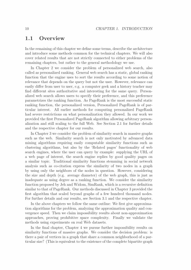
The Companion similarity function was introduced by Jeff Dean and MonikaHenzinger in 1999 [38] based on the ideas from the HITS ranking algorithm.Their method searches for the most similar pages to a query page v and assignsimilarity scores to them:
1. Using heuristics we identify the subgraph representing the neighborhoodof page v. This includes pi in-neighbors of v; pio out-neighbors of eachof them; po out-neighbors of v and poi in-neighbors of each of them.The four parameters are tuned manually, and wherever the neighbor setexceeds the respective parameter value, we select a uniform random presp
element subset.
2. We take the subgraph spanned by the selected nodes. We merge thenodes that have their out-neighborhood overlapping by 95%.

26 CHAPTER 1. INTRODUCTION
3. We run the HITS algorithm on the derived graph. We employ a slightmodification to the original algorithm that handles multiple edges be-tween nodes with a proper weighting.
4. Finally we use the authority scores of the nodes to rank them.
Apart from the extra cleaning steps this is in practice a local version of theHITS ranking algorithm, computing hub- and authority-scores in the smallneighborhood of the query page v. Since the neighborhood is local to the nodein question, this method does not suffer from the topical drift of the globalHITS ranking algorithm.
Unfortunately this method cannot be applied to the entire web graph basedon our computing model (see Section 1.6). The main problem is that in orderto select the subgraph spanned by this neighborhood we need to make manyrandom accesses into the database storing the web graph. This is feasibleonly if we have memory proportional to the size of the complete web graph,which is often prohibitively expensive. Recent results have shown methodsthat are able to store a significant portion of the web graph in memory usingsophisticated compression methods [2, 16], but performing random access oncompressed data is also costly.
1.9.2 The SimRank similarity function
The SimRank similarity function, which is one of the central subject of studyin Chapter 3, was introduced by Glen Jeh and Jennifer Widom in 2002 [74].SimRank is the recursive refinement of the co-citation function, similarly asPageRank is the recursive refinement of in-degree ranking.
The key idea behind SimRank is the following:
The similarity of a pair of web-pages is the average similarity ofthe pages linking to them.
Definition 3 (SimRank equations).
sim(u, u) = 1sim(u, v) = 0, if u 6= v and (I(u) = ∅ or I(v) = ∅)sim(u, v) = c
|I(u)|·|I(v)|
∑u′∈I(u)
∑v′∈I(v) sim(u′, v′), otherwise,
where c ∈ (0, 1) is a constant, u, v are nodes in the graph, and I(u) is the setof nodes linking to u.
For V nodes this means a linear equation system with V 2 equation and V 2
variables. Since c < 1 the norm of the equation matrix is less, than 1 and it iseasy to see that the equation system has a unique solution. In theory it is fairlyeasy to come up with this solution, since from an arbitrary starting point aniteration over the equation system will converge to the solution exponentially.

1.9. ITERATIVE LINK-BASED SIMILARITY FUNCTIONS 27
In practice nevertheless, just in order to be able to do one iteration on theequation system we would need to store the values of all the variables. With aweb graph of a mere 1 billion nodes this means 1018 values to store, which is acompletely unrealistic requirement: we would need billions of hard drives of thehighest capacity to date. Even with pruning during the iteration (rounding allvalues smaller than a threshold to zero [74]) the naive iteration-based methodis only applicable to graphs of a few hundred thousand vertices.

28 CHAPTER 1. INTRODUCTION

Chapter 2Personalized Web Search
2.1 Introduction
The idea of topic sensitive or personalized ranking appears since the beginningof the success story of Google’s PageRank [21, 95] and other hyperlink-basedquality measures [82, 19]. Topic sensitivity is either achieved by precomputingmodified measures over the entire Web [63] or by ranking the neighborhoodof pages containing the query word [82]. These methods however work onlyfor restricted cases or when the entire hyperlink structure fits into the mainmemory.
In this chapter we address the computational issues [63, 75] of personalizedPageRank [95]. Just as all hyperlink based ranking methods, PageRank isbased on the assumption that the existence of a hyperlink u → v implies thatpage u votes for the quality of v. Personalized PageRank (PPR) enters userpreferences by assigning more importance to edges in the neighborhood ofcertain pages at the user’s selection. Unfortunately the naive computation ofPPR requires a power iteration algorithm over the entire web graph, makingthe procedure infeasible for an on-line query response service.
Earlier personalized PageRank (PPR) algorithms restricted personaliza-tion to a few topics [63], a subset of popular pages [75] or to hosts [77]; see[66] for an analytical comparison of these methods. The state of the art HubDecomposition algorithm [75] can answer queries for up to some 100,000 per-sonalization pages, an amount relatively small even compared to the numberof categories in the Open Directory Project [94].
In contrast to earlier PPR algorithms, we achieve full personalization: ourmethod enables on-line serving of personalization queries for any set of pages.We introduce a novel, scalable Monte Carlo algorithm that precomputes a com-pact database. As described in Section 2.2, the precomputation uses simulatedrandom walks, and stores the ending vertices of the walks in the database. PPRis estimated on-line with a few database accesses.
The price that we pay for full personalization is that our algorithm is ran-
29

30 CHAPTER 2. PERSONALIZED WEB SEARCH
domized and less precise than power-iteration-like methods; the formal anal-ysis of the error probability is discussed in Section 2.3. We theoretically andexperimentally show that we give sufficient information for all possible person-alization pages while adhering to the strong implementation requirements of alarge-scale web search engine.
According to Section 2.4, some approximation seems to be inavoidable sincethe exact personalization requires a database as large as Ω(V 2) bits in worstcase over graphs with V vertices. Though no worst case theorem applies tothe webgraph or one particular graph, the theorems show the nonexistence ofa general exact algorithm that computes a linear sized database on any graph.To achieve full personalization in future research, one must hence either exploitspecial features of the webgraph or relax the exact problem to an approximateone as in our scenario. Of independent interest is another consequence of ourlower bounds that there is indeed a large amount of information in personalizedPageRank vectors since, unlike uniform PageRank, it can hold information ofsize quadratic in the number of vertices.
In Section 2.5 we experimentally analyze the precision of approximation onthe Stanford WebBase graph and conclude that our randomized approxima-tion method provides sufficiently good approximation for the top personalizedPageRank scores.
Though our approach might give results of inadequate precision in certaincases (for example for pages with large neighborhood), the available person-alization algorithms can be combined to resolve these issues. For example wecan precompute personalization vectors for certain topics by topic-sensitivePR [63], for popular pages with large neighborhoods by the hub skeleton al-gorithm [75]), and use our method for those millions of pages not covered sofar. This combination gives adequate precision for most queries with largeflexibility for personalization.
2.1.1 Related Results
We compare our method with known personalized PageRank approaches aslisted in Table 2.1 to conclude that our algorithm is the first that can handleon-line personalization on arbitrary pages. Earlier methods in contrast eitherrestrict personalization or perform non-scalable computational steps such aspower-iteration in query time or quadratic disk usage during the precomputa-tion phase. The only drawback of our algorithm compared to previous ones isthat its approximation ratio is somewhat worse than that of the power iterationmethods.
The first known algorithm [95] (Naive in Table 2.1) simply takes the per-sonalization vector as input and performs power iteration at query time. Thisapproach is clearly infeasible for on-line queries. One may precompute thepower iterations for a well selected set of personalization vectors as in theTopic Sensitive PageRank [63]; however full personalization in this case re-

2.1. INTRODUCTION 31
quires t = V precomputed vectors yielding a database of size V 2 for V webpages. The current size V ≈ 109 −1010 hence makes full personalization infea-sible.
The third algorithm of Table 2.1, BlockRank [77] restricts personalizationto hosts. While the algorithm is attractive in that the choice of personal-ization is fairly general, a reduced number of power iterations still need tobe performed at query time that makes the algorithm infeasible for on-linequeries.
The remarkable Hub Decomposition algorithm [75] restricts the choice ofpersonalization to a set H of top ranked pages. Full personalization howeverrequires H to be equal to the set of all pages, thus V 2 space is required again.The algorithm can be extended by the Web Skeleton [75] to lower estimate thepersonalized PageRank vector of arbitrary pages by taking into account onlythe paths that goes through the set H . Unfortunately, if H does not overlapthe few-step neighborhood of a page, then the lower estimation provides poorapproximation for the personalized PageRank scores.
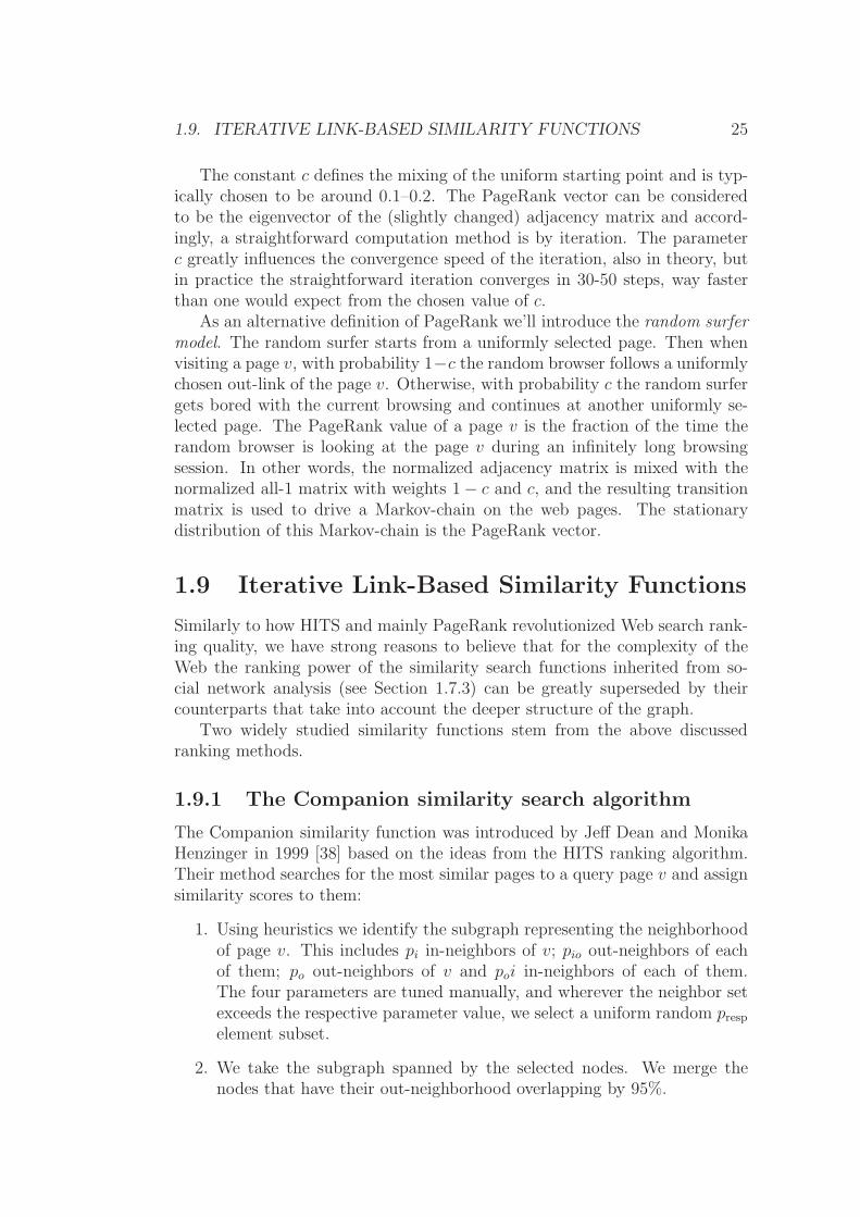
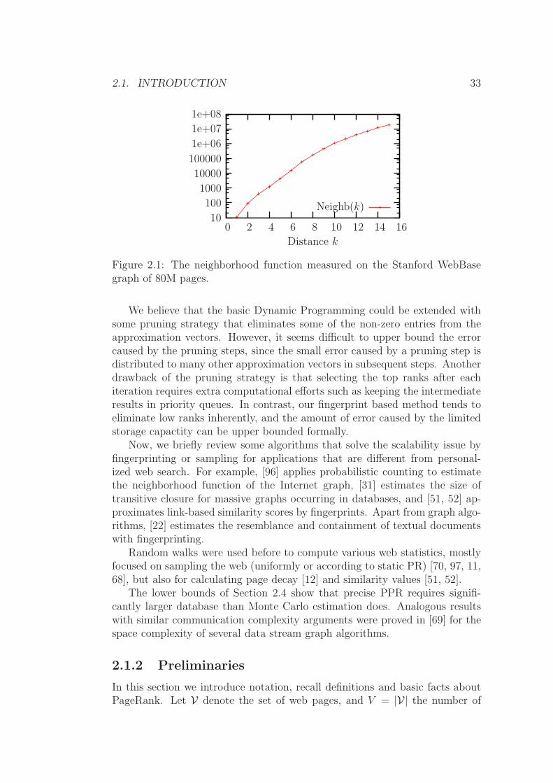
The Dynamic Programming approach [75] provides full personalization byprecomputing and storing sparse approximate personalized PageRank vectors.The key idea is that in a k-step approximation only vertices within distancek have nonzero value. However the rapid expansion of the k-neighborhoodsincreases disk requirement close to V 2 after a few iterations that limits the us-ability of this approach. Furthermore, a possible external memory implemen-tation would require significant additional disk space. The space requirementsof Dynamic Programming for a single vertex is given by the average neighbor-hood size Neighb(k) within distance k as seen in Fig. 2.1. The average size ofthe sparse vectors exceeds 1000 after k ≥ 4 iterations, and on average 24% ofall vertices are reached within k = 15 steps1. For example the disk require-ment for k = 10 iterations is at least Neighb(k) · V = 1, 075, 740 · 80M ≈ 344Terabytes. Note that the best upper bound of the approximation is still(1 − c)10 = 0.8510 ≈ 0.20 measured by the L1-norm.
1The neighborhood function was computed by combining the size estimation methodof [31] with our external memory algorithm discussed in [52].

32C
HA
PT
ER
2.P
ER
SO
NA
LIZ
ED
WE
BSE
AR
CH
Method Personalization Limits of scalability Postitive aspects Negative aspects
Naive [95] any page power iteration in query-time
infeasible to serve on-linepersonalization
Topic-SensitivePageRank [63]
restricted to linear combi-nation of t topics, e.g. t =16
t · V disk space required distributed computing
BlockRank[77]
restricted to personalizeon hosts
power iteration in query-time
reduced number of poweriterations, distributedcomputing
infeasible to serve on-linepersonalization
Hub Decom-position [75]
restricted to personalizeon the top H ranked pages,practically H ≤ 100K
H2 disk space required,H partial vectors aggre-gated in query time
compact encoding of H
personalized PR vectors
Basic DynamicProgramming[75]
any page V · Neighb(k) disk spacerequired for k iterations,where Neighb(k) growsfast in k
infeasible to perform morethan k = 3, 4 iterationswithin reasonable disk size
Fingerprint(this paper)
any page no limitation linear-size (N · V ) disk re-quired, distributed compu-tation
lower precision approxima-tion
Table 2.1: Analytical comparison of personalized PageRank algorithms. V denotes the number of all pages.
2.1. INTRODUCTION 33
Neighb(k)
Distance k
1614121086420
1e+08
1e+07
1e+06
100000
10000
1000
100
10
Figure 2.1: The neighborhood function measured on the Stanford WebBasegraph of 80M pages.
We believe that the basic Dynamic Programming could be extended withsome pruning strategy that eliminates some of the non-zero entries from theapproximation vectors. However, it seems difficult to upper bound the errorcaused by the pruning steps, since the small error caused by a pruning step isdistributed to many other approximation vectors in subsequent steps. Anotherdrawback of the pruning strategy is that selecting the top ranks after eachiteration requires extra computational efforts such as keeping the intermediateresults in priority queues. In contrast, our fingerprint based method tends toeliminate low ranks inherently, and the amount of error caused by the limitedstorage capactity can be upper bounded formally.
Now, we briefly review some algorithms that solve the scalability issue byfingerprinting or sampling for applications that are different from personal-ized web search. For example, [96] applies probabilistic counting to estimatethe neighborhood function of the Internet graph, [31] estimates the size oftransitive closure for massive graphs occurring in databases, and [51, 52] ap-proximates link-based similarity scores by fingerprints. Apart from graph algo-rithms, [22] estimates the resemblance and containment of textual documentswith fingerprinting.
Random walks were used before to compute various web statistics, mostlyfocused on sampling the web (uniformly or according to static PR) [70, 97, 11,68], but also for calculating page decay [12] and similarity values [51, 52].
The lower bounds of Section 2.4 show that precise PPR requires signifi-cantly larger database than Monte Carlo estimation does. Analogous resultswith similar communication complexity arguments were proved in [69] for thespace complexity of several data stream graph algorithms.
2.1.2 Preliminaries
In this section we introduce notation, recall definitions and basic facts aboutPageRank. Let V denote the set of web pages, and V = |V| the number of

34 CHAPTER 2. PERSONALIZED WEB SEARCH
pages. The directed graph with vertex set V and edges corresponding to thehyperlinks will be referred to as the web graph. Let A denote the adjacencymatrix of the webgraph with normalized rows and c ∈ (0, 1) the teleportationprobability. In addition, let ~r be the so called preference vector inducing aprobability distribution over V. PageRank vector ~p is defined as the solutionof the following equation [95]
~p = (1 − c) · ~pA + c · ~r .
If ~r is uniform over V, then ~p is referred to as the global PageRank vector.For non-uniform ~r the solution ~p will be referred to as personalized PageRankvector of ~r denoted by PPV(~r). The special case when for some page u the uth
coordinate of ~r is 1 and all other coordinates are 0, the PPV will be referredto as the individual PageRank vector of u denoted by PPV(u). We will alsorefer to this vector as the personalized PageRank vector of u. Furthermore thevth coordinate of PPV(u) will be denoted by PPV(u, v).
Theorem 4 (Linearity, [63]). For any preference vectors ~r1, ~r2, and positiveconstants α1, α2 with α1 + α2 = 1 the following equality holds:
PPV(α1 · ~r1 + α2 · ~r2) = α1 · PPV(~r1) + α2 · PPV(~r2).
Linearity is a fundamental tool for scalable on-line personalization, since ifPPV is available for some preference vectors, then PPV can be easily computedfor any combination of the preference vectors. Particularly, for full personaliza-tion it suffices to compute individual PPV(u) for all u ∈ V, and the individualPPVs can be combined on-line for any small subset of pages. Therefore inthe rest of this chapter we investigate algorithms to make all individual PPVsavailable on-line.
The following statement will play a central role in our PPV estimations.The theorem provides an alternate probabilistic characterization of individualPageRank scores.2
Theorem 5 ( [75, 50] ). Suppose that a number L is chosen at random withprobability PrL = i = c(1 − c)i for i = 0, 1, 2, . . . Consider a random walkstarting from some page u and taking L steps. Then for the vth coordinatePPV(u, v) of vector PPV(u)
PPV(u, v) = Prthe random walk ends at page v.
2.2 Personalized PageRank algorithm
In this section we will present a new Monte-Carlo algorithm to compute ap-proximate values of personalized PageRank utilizing the above probabilis-tic characterization of PPR. We will compute approximations of each of the
2Notice that this characterization slightly differs from the random surfer formulation [95]of PageRank.

2.2. PERSONALIZED PAGERANK ALGORITHM 35
PageRank vectors personalized on a single page, therefore by the linearitytheorem we achieve full personalization.
Our algorithm utilizes the simulated random walk approach that has beenused recently for various web statistics and IR tasks [12, 51, 11, 70, 97].
Definition 6 (Fingerprint path). A fingerprint path of a vertex u is a randomwalk starting from u; the length of the walk is of geometric distribution ofparameter c, i.e., after each step the walk takes a further step with probability1 − c and ends with probability c.
Definition 7 (Fingerprint). A fingerprint of a vertex u is the ending vertexof a fingerprint path of u.
By Theorem 5 the fingerprint of page u, as a random variable, has thedistribution of the personalized PageRank vector of u. For each page u we willcalculate N independent fingerprints by simulating N independent randomwalks starting from u and approximate PPV(u) with the empirical distributionof the ending vertices of these random walks. These fingerprints will constitutethe index database, thus the size of the database is N · V . The output rankingwill be computed at query time from the fingerprints of pages with positivepersonalization weights using the linearity theorem.
To increase the precision of the approximation of PPV(u) we will use thefingerprints that were generated for the neighbors of u, as described in Sec-tion 2.2.3.
The challenging problem is how to scale the indexing, i.e., how to generateN independent random walks for each vertex of the web graph. We assumethat the edge set can only be accessed as a data stream, sorted by the sourcepages, and we will count the database scans and total I/O size as the efficiencymeasure of our algorithms. Though with the latest compression techniques[17] the entire web graph may fit into main memory, we still have a significantcomputational overhead for decompression in case of random access. Undersuch assumption it is infeasible to generate the random walks one-by-one, asit would require random access to the edge-structure.
We will consider two computational environments here: a single computerwith constant random access memory in case of the external memory model,and a distributed system with tens to thousands of medium capacity computers[37]. Both algorithms use similar techniques to the respective I/O efficientalgorithms computing PageRank [30].
As the task is to generate N independent fingerprints, the single computersolution can be trivially parallelized to make use of a large cluster of machines,too. (Commercial web search engines have up to thousands of machines attheir disposal.) Also, the distributed algorithm can be emulated on a singlemachine, which may be more efficient than the external memory approachdepending on the graph structure.

36 CHAPTER 2. PERSONALIZED WEB SEARCH
Algorithm 2.2.1 Indexing (external memory method)
N is the required number of fingerprints for each vertex. The array Paths holdspairs of vertices (u, v) for each partial fingerprint in the calculation, interpretedas (PathStart,PathEnd). The teleportation probability of PPR is c. The arrayFingerprint[u] stores the fingerprints computed for a vertex u.
for each web page u dofor i := 1 to N do
append the pair (u, u) to array Paths /*start N fingerprint paths fromnode u: initially PathStart=PathEnd= u*/
Fingerprint[u] := ∅while Paths 6= ∅ do
sort Paths by PathEnd /*use an external memory sort*/for all (u, v) in Paths do /*simultaneous scan of the edge set and Paths*/
w := a random out-neighbor of vif random()< c then /*with probability c this fingerprint path endshere*/
add w to Fingerprint[u]delete the current element (u, v) from Paths
else /*with probability 1 − c the path continues*/update the current element (u, v) of Paths to (u, w)
2.2.1 External memory indexing
We will incrementally generate the entire set of random walks simultaneously.Assume that the first k vertices of all the random walks of length at least kare already generated. At any time it is enough to store the starting and thecurrent vertices of the fingerprint path, as we will eventually drop all the nodeson the path except the starting and the ending nodes. Sort these pairs by theending vertices. Then by simultaneously scanning through the edge set andthis sorted set we can have access to the neighborhoods of the current endingvertices. Thus each partial fingerprint path can be extended by a next vertexchosen from the out-neigbors of the ending vertex uniformly at random. Foreach partial fingerprint path we also toss a biased coin to determine if it hasreached its final length with probability c or has to advance to the next roundwith probability 1 − c. This algorithm is formalized as Algorithm 2.2.1.
The number of I/O operations the external memory sorting takes is
D logM D
where D is the database size and M is the available main memory. Thus theexpected I/O requirement of the sorting parts can be upper bounded by
∞∑
k=0
(1 − c)kNV logM((1 − c)kNV ) =1
cNV logM(NV ) − Θ(NV )

2.2. PERSONALIZED PAGERANK ALGORITHM 37
using the fact that after k rounds the expected size of the Paths array is (1 −c)kNV . Recall that V and N denote the numbers of vertices and fingerprints,respectively.
We need a sort on the whole index database to avoid random-access writesto the Fingerprint arrays. Also, upon updating the PathEnd variables we donot write the unsorted Paths array to disk, but pass it directly to the nextsorting stage. Thus the total I/O is at most 1
cNV logM NV plus the necessary
edge-scans.
Unfortunately this algorithm apparently requires as many edge-scans as thelength of the longest fingerprint path, which can be very large: Prthe longestfingerprint is shorter, than L = (1 − (1 − c)L)N ·V . Thus instead of scanningthe edges in the final stages of the algorithm, we will change strategy when thePaths array has become sufficiently small. Assume a partial fingerprint pathhas its current vertex at v. Then upon this condition the distribution of theend of this path is identical to the distribution of the end of any fingerprintof v. Thus to finish the partial fingerprint we can retrieve an already finishedfingerprint of v. Although this decreases the number of available fingerprintsfor v, this results in only a very slight loss of precision.3
Another approach to this problem is to truncate the paths at a given lengthL and approximate the ending distribution with the static PageRank vector,as described in Section 2.2.3.
2.2.2 Distributed index computing
In the distributed computing model we will invert the previous approach, andinstead of sorting the path ends to match the edge set we will partition theedge set of the graph in such a way that each participating computer can holdits part of the edges in main memory. So at any time if a partial fingerprintwith current ending vertex v requires a random out-edge of v, it can ask therespective computer to generate one. This will require no disk access, onlynetwork transfer.
More precisely, each participating computer will have several queues hold-ing (PathStart, PathEnd) pairs: one large input queue, and for each computerone small output queue preferably with the size of a network packet.
The computation starts with each computer filling their own input queuewith N copies of the initial partial fingerprints (u, u), for each vertex u be-longing to the respective computer in the vertex partition.
Then in the input queue processing loop a participating computer takes thenext input pair, generates a random out-edge from PathEnd, decides whetherthe fingerprint ends there, and if it does not, then places the pair in theoutput queue determined by the next vertex just generated. If an output queue
3Furthermore, we can be prepared for this event: the distribution of these v vertices willbe close to the static PageRank vector, thus we can start with generating somewhat morefingerprints for the vertices with high PR values.
38 CHAPTER 2. PERSONALIZED WEB SEARCH
Algorithm 2.2.2 Indexing (distributed computing method)
The algorithm of one participating computer. Each computer is responsible fora part of the vertex set, keeping the out-edges of those vertices in main memory.For a vertex v, part(v) is the index of the computer that has the out-edges of v.The queues hold pairs of vertices (u, v), interpreted as (PathStart, PathEnd).
for u with part(u) = current computer dofor i := 1 to N do
insert pair (u, u) into InQueue /*start N fingerprint paths from nodeu: initially PathStart=PathEnd= u*/
while at least one queue is not empty do /*some of the fingerprints are stillbeing calculated*/
get an element (u, v) from InQueue/*if empty, wait until an element ar-rives.*/w := a random out-neighbor of v/*prolong the path; we have the out-edges of v in memory*/if random()< c then /*with probability c this fingerprint path endshere*/
add w to the fingerprints of uelse /*with probability 1 − c the path continues*/
o := part(w) /*the index of the computer responsible for continuing thepath*/insert pair (u, w) into the InQueue of computer o
transmit the finished fingerprints to the proper computers for collecting andsorting.
reaches the size of a network packet’s size, then it is flushed and transferredto the input queue of the destination computer. Notice that either we haveto store the partition index for those v vertices that have edges pointing toin the current computer’s graph, or part(v) has to be computable from v,for example by renumbering the vertices according to the partition. For sakeof simplicity the output queue management is omitted from the pseudo-codeshown as Algorithm 2.2.2.
The total size of all the input and output queues equals the size of the Pathsarray in the previous approach after the respective number of iterations. Theexpected network transfer can be upper bounded by
∑∞n=0(1−c)nNV = 1
cNV ,
if every fingerprint path needs to change computer in each step.
In case of the webgraph we can significantly reduce the above amount ofnetwork transfer with a suitable partition of the vertices. The key idea is tokeep each domain on a single computer, since the majority of the links areintra-domain links as reported in [77, 41].
We can further extend the above heuristical partition to balance the com-putational and network load among the participating computers in the net-work. One should use a partition of the pages such that the amount of global

2.2. PERSONALIZED PAGERANK ALGORITHM 39
PageRank is ditributed uniformly across the computers. The reason is that theexpected value of the total InQueue hits of a computer is proportional to thetotal PageRank score of vertices belonging to that computer. Thus when usingsuch a partition, the total switching capacity of the network is challenged, notthe capacity of the individual network links.
2.2.3 Query processing
The basic query algorithm is as follows: to calculate PPV(u) we load theending vertices of the fingerprints for u from the index database, calculate theempirical distribution over the vertices, multiply it with 1−c, and add c weightto vertex u. This requires one database access (disk seek).
To reach a precision beyond the number of fingerprints saved in the data-base we can use the recursive property of PPV, which is also referred to as thedecomposition theorem in [75]:
PPV(u) = c1u +(1 − c)1
|O(u)|∑
v∈O(u)
PPV(v)
where 1u denotes the measure concentrated at vertex u (i.e., the unit vectorof u), and O(u) is the set of out-neighbors of u.
This gives us the following algorithm: upon a query u we load the fin-gerprints for u, the set of out-neighbors O(u), and the fingerprints for thevertices of O(u). From this set of fingerprints we use the above equation toapproximate PPV(u) using a higher amount of samples, thus achieving higherprecision. This is a tradeoff between query time (database accesses) and pre-cision: with |O(u)| database accesses we can approximate the vector from|O(u)| · N samples. We can iterate this recursion, if want to have even moresamples. We mention that such query time iterations are analogous to thebasic dynamic programming algorithm of [75]. The main difference is that inour case the iterations are used to increase the number of fingerprints ratherthan the maximal length of the paths taken into account as in [75].
The increased precision is essential in approximating the PPV of a pagewith large neighborhood, as from N samples at most N pages will have positiveapproximated PPR values. Fortunately, this set is likely to contain the pageswith highest PPR scores. Using the samples of the neighboring vertices willgive more adequate result, as it will be formally analyzed in the next section.
We could also use the expander property of the web graph: after not somany random steps the distribution of the current vertex will be close to thestatic PageRank vector. Instead of allowing very long fingerprint paths wecould combine the PR vector with coefficient (1− c)L+1 to the approximationand drop all fingerprints longer than L. This would also solve the problem ofthe approximated individual PPR vectors having many zeros (in those verticesthat have no fingerprints ending there). The indexing algorithms would benefitfrom this truncation, too.

40 CHAPTER 2. PERSONALIZED WEB SEARCH
There is a further interesting consequence of the recursive property. If it isknown in advance that we want to personalize over a fixed (maybe large) setof pages, we can introduce an artificial node into the graph with the respectiveset of neighbors to generate fingerprints for that combination.
2.3 How Many Fingerprints are Needed?
In this section we will discuss the convergence of our estimates, and analyzethe required amount of fingerprints for proper precision.
It is clear by the law of large numbers that as the number of fingerprintsN → ∞, the estimate PPV(u) converges to the actual personalized PageRankvector PPV(u). To show that the rate of convergence is exponential, recall thateach fingerprint of u ends at v with probability PPV(u, v), where PPV(u, v)
denotes the vth coordinate of PPV(u). Therefore N · PPV(u, v), the numberof fingerprints of u that ends at v, has binomial distribution with parametersN and PPV(u, v). Then Chernoff’s inequality yields the following bound onthe error of over-estimating PPV(u, v) and the same bound holds for under-estimation:
PrPPV(u, v) > (1 + δ) PPV(u, v)= PrN PPV(u, v) > N(1 + δ) PPV(u, v)≤ e−N ·PPV(u,v)·δ2/4.
Actually, for applications the exact values are not necessary. We onlyneed that the ordering defined by the approximation match fairly closely theordering defined by the personalized PageRank values. In this sense we haveexponential convergence too:
Theorem 8. For any vertices u, v, w consider PPV(u) and assume that:
PPV(u, v) > PPV(u, w)
Then the probability of interchanging v and w in the approximate ranking tendsto 0 exponentially in the number of fingerprints used.
Theorem 9. For any ǫ, δ > 0 there exists an N0 such that for any N ≥N0 number of fingerprints, for any graph and any vertices u, v, w such thatPPV(u, v) − PPV(u, w) > δ, the inequality PrPPV(u, v) < PPV(u, w) < ǫholds.
Proof. We prove both theorems together. Consider a fingerprint of u andlet Z be the following random variable: Z = 1, if the fingerprint ends in v,Z = −1 if the fingerprint ends in w, and Z = 0 otherwise. Then EZ =PPV(u, v) − PPV(u, w) > 0. Estimating the PPV values from N fingerprints

2.4. LOWER BOUNDS FOR PPR DATABASE SIZE 41
the event of interchanging v and w in the rankings is equivalent to takingN independent Zi variables and having
∑Ni=1 Zi < 0. This can be upper
bounded using Bernstein’s inequality and the fact that Var(Z) = PPV(u, v)+PPV(u, w) − (PPV(u, v) − PPV(u, w))2 ≤ PPV(u, v) + PPV(u, w):
Pr 1N
∑Ni=1 Zi < 0 ≤ e
−N (EZ)2
2 Var(Z)+4/3EZ
≤ e−N (PPV(u,v)−PPV(u,w))2
10/3 PPV(u,v)+2/3 PPV(u,w)
≤ e−0.3N(PPV(u,v)−PPV(u,w))2
From the above inequality both theorems follow.
The first theorem shows that even a modest amount of fingerprints areenough to distinguish between the high, medium and low ranked pages ac-cording to the personalized PageRank scores. However, the order of the lowranked pages will usually not follow the PPR closely. This is not surpris-ing, and actually a significant problem of PageRank itself, as [86] showed thatPageRank is unstable around the low ranked pages, in the sense that withsmall perturbation of the graph a very low ranked page can jump in the rank-ing order somewhere to the middle.
The second statement has an important theoretical consequence. When weinvestigate the asymptotic growth of database size as a function of the graphsize, the number of fingerprints remains constant for fixed ǫ and δ.
2.4 Lower Bounds for PPR Database Size
In this section we will prove several worst case lower bounds on the complex-ity of personalized PageRank problem. The lower bounds suggest that theexact computation and storage of all personalized PageRank vectors is infea-sible for massive graphs. Notice that the theorems cannot be applied to onespecific input such as the webgraph. The theorems show that for achieving fullpersonalization the web-search community should either utilize some specificproperties of the webgraph or relax the exact problem to an approximate oneas in our scenario.
In particular, we will prove that the necessary index database size of afully personalized PageRank algorithm computing exact scores must be atleast Ω(V 2) bits in worst case, and if personalizing only for H nodes, the sizeof the database is at least Ω(H · V ). If we allow some small error probabilityand approximation, then the lower bound for full personalization is linear inV , which is achieved by our algorithm of Section 2.2.
More precisely we will consider two-phase algorithms: in the first phase thealgorithm has access to the graph and has to compute an index database. Inthe second phase the algorithm gets a query of arbitrary vertices u, v (and w),and it has to answer based on the index database, i.e., the algorithm cannotaccess the graph during query-time. An f(V ) worst case lower bound on the

42 CHAPTER 2. PERSONALIZED WEB SEARCH
database size holds, if for any two-phase algorithm there exists a graph onV vertices such that the algorithm builds a database of size f(V ) in the firstphase.
In the above introduced two-phase model, we will consider the followingtypes of queries:
(1) Exact: Calculate PPV(u, v), the vth element of the personalized PageRankvector of u.
(2) Approximate: Estimate PPV(u, v) with a PPV(u, v) such, that for fixedǫ, δ > 0
Pr|PPV(u, v) − PPV(u, v)| < δ ≥ 1 − ǫ
(3) Positivity: Decide whether PPV(u, v) is positive with error probability atmost ǫ.
(4) Comparison: Decide in which order v and w are in the personalized rankof u with error probability at most ǫ.
(5) ǫ–δ comparison: For fixed ǫ, δ > 0 decide the comparison problem witherror probability at most ǫ, if |PPV(u, v) − PPV(u, w)| > δ holds.
(6) φ–ǫ–δ top query : given the vertex u, with probability 1 − ǫ compute theset of vertices W which have personalized PPR values according to vertexu greater than φ. Precisely we require the following:
∀w ∈ V : PPV(u, w) ≥ φ ⇒ w ∈ W
∀w ∈ W : PPV(u, w) ≥ φ − δ
Our tool towards the lower bounds will be the asymmetric communicationcomplexity game bit-vector probing [69]: there are two players A and B. PlayerA has an m-bit vector x, player B has a number y ∈ 1, 2, . . . , m, and theirtask is to compute the function f(x, y) = xy, i.e., the output is the yth bit ofthe input vector. To compute the proper output they have to communicate,and communication is restricted in the direction A → B. The one-way com-munication complexity [84] of this function is the required bits of transfer inthe worst case for the best protocol.
Theorem 10 ([69]). Any protocol that outputs the correct answer to the bit-vector probing problem with probability at least 1+γ
2must transmit at least γm
bits in worst case.
Now we are ready to prove our lower bounds. In all our theorems we assumethat personalization is calculated for H vertices, and there are V vertices intotal. Notice that in the case of full personalization H = V holds.
Theorem 11. Any algorithm solving the positivity problem (3) must use anindex database of size Ω((1 − 2ǫ)HV ) bits in worst case.

2.4. LOWER BOUNDS FOR PPR DATABASE SIZE 43
Proof. Set 1+γ2
= 1 − ǫ. We give a communication protocol for the bit-vectorprobing problem. Given an input bit-vector x we will create a graph, that‘codes’ the bits of this vector. Player A will create a PPV database on thisgraph, and transmit this database to B. Then Player B will use the positivityquery algorithm for some vertices (depending on the requested number y) suchthat the answer to the positivity query will be the yth bit of the input vectorx. Thus if the algorithm solves the PPV indexing and positivity query witherror probability ǫ, then this protocol solves the bit-vector probing problemwith probability 1+γ
2, so the transferred index database’s size is at least γm.
For the H ≤ V/2 case consider the following graph: let u1, . . . , uH denotethe vertices for whose the personalization is calculated. Add v1, v2, . . . , vn
more vertices to the graph, where n = V − H . Let the input vector’s size bem = H · n. In our graph each vertex vj has a loop, and for each 1 ≤ i ≤ Hand 1 ≤ j ≤ n the edge (ui, vj) is in the graph iff bit (i − 1)n + j is set in theinput vector.
For any number 1 ≤ y ≤ m let y = (i−1)n+j; the personalized PageRankvalue PPV(ui, vj) is positive iff (ui, vj) edge was in the graph, thus iff bit y wasset in the input vector. If H ≤ V/2 the theorem follows since n = V − H =Ω(V ) holds implying that m = H · n = Ω(H · V ) bits are ‘coded’.
Otherwise, if H > V/2 the same construction proves the statement withsetting H = V/2.
Corollary 12. Any algorithm solving the exact PPV problem (1) must havean index database of size Ω(H · V ) bits in worst case.
Theorem 13. Any algorithm solving the approximation problem (2) needs anindex database of Ω(1−2ǫ
δH) bits on a graph with V = H + Ω(1
δ) vertices in
worst case. If V = H +O(1δ), then the index database requires Ω((1−2ǫ)HV ).
Proof. We will modify the construction of Theorem 11 for the approximationproblem. We have to achieve that when a bit is set in the input graph, then thequeried PPV(ui, vj) value should be at least 2δ, so that the approximation willdecide the positivity problem, too. If there are k edges incident to vertex ui
in the constructed graph, then each target vertex vj has weight PPV(ui, vj) =1−ck
. For this to be over 2δ we can have at most n = 1−c2δ
possible v1, . . . , vn
vertices. With 1+γ2
= 1 − ǫ the first statement of the theorem follows.For the second statement the original construction suffices.
This radical drop in the storage complexity is not surprising, as our approx-imation algorithm achieves this bound (up to a logarithmic factor): for fixedǫ, δ we can calculate the necessary number of fingerprints N , and then for eachvertex in the personalization we store exactly N fingerprints, independently ofthe graph’s size.
Using somewhat more extra nodes in the graph we can prove an evenstronger lower bound:

44 CHAPTER 2. PERSONALIZED WEB SEARCH
Theorem 14. Any algorithm solving the approximation problem (2) needs adatabase of Ω(1
δlog 1
ǫ·H) bits in worst case, when the graph has at least H+ 1−c
8δǫ
nodes.
Proof. We prove the theorem by reducing the bit vector probing problem tothe ǫ–δ approximation. Given a vector x of m = Ω(1
δ· log 1
ǫ·H) bits, player A
will construct a graph and compute a PPR database with the indexing phaseof the ǫ–δ approximation algorithm. Then A transmits this database to B.Player B will perform a sequence of queries such that the required bit xy willbe computed with error probability 1
4. The above outlined protocol solves the
bit vector probing with error probability 14. Thus the database size that is
equal to the number of transmitted bits is Ω(m) = Ω(1δ· log 1
ǫ· H) in worst
case by Theorem 10. It remains to show the details of the graph constructionon A’s side and the query algorithm on B’s side.
Given a vector x of m = 1−c2δ
· log 14ǫ· H bits, A constructs the “bipartite”
graph with vertex set ui : i = 1, . . . , H∪vj,k : j = 1, . . . , 1−c2δ
, k = 1, . . . , 14ǫ.
For the edge set, x is partitioned into 1−c2δ
· H blocks, where each block bi,j
contains log 14ǫ
bits for i = 1, . . . , H , j = 1, . . . , 1−c2δ
. Notice that each bi,j canbe regarded as a binary encoded number with 0 ≤ bi,j < 1
4ǫ. To encode x
into the graph, A adds an edge (ui, vj,k) iff bi,j = k, and also attaches a self-loop to each vj,k. Thus the 1−c
2δedges outgoing from ui represent the blocks
bi,1, . . . , bi,(1−c)/2δ.After constructing the graph A computes an ǫ–δ approximation PPR data-
base with personalization available on u1, . . . , uH, and sends the database toB, who computes the yth bit xy as follows. Since B knows which of the blockscontains xy it is enough to compute bi,j for suitably chosen i, j. The key prop-erty of the graph construction is that PPV(ui, vj,k) = 1−c
|O(ui)|= 2δ iff bi,j = k
otherwise PPV(ui, vj,k) = 0. Thus B computes PPV(ui, vj,k) for k = 1, . . . , 14ǫ
by the second phase of the ǫ–δ approximation algorithm. If all PPV(ui, vj,k) are
computed with |PPV(ui, vj,k)− PPV(ui, vj,k)| ≤ δ, then bi,j containing xy willbe calculated correctly. By the union bound the probability of miscalculatingany of PPV(ui, vj,k) is at most 1
4ǫ· ǫ = 1
4.
We now move on to other query types.
Theorem 15. Any algorithm solving the comparison problem (4) requires anindex database of Ω((1 − 2ǫ)HV ) bits in worst case.
Proof. We will modify the graph of Theorem 11 so that the existence of thespecific edge can be queried using the comparison problem. To achieve thiswe will introduce a third set of vertices w1, . . . , wn in the graph construction,such that wj is the complement of vj : A puts the edge (ui, wj) in the graph iff(ui, vj) was not an edge, which means bit (i− 1)n + j was not set in the inputvector.
Then upon query for bit y = (i− 1)n + j, consider PPV(ui). In this vectorexactly one of vj , wj will have positive weight (depending on the input bit xy),

2.5. EXPERIMENTS 45
thus the comparison query PPV(ui, vj) > PPV(ui, wj) will yield the requiredoutput for the bit-vector probing problem.
Corollary 16. Any algorithm solving the ǫ–δ comparison problem (5) needsan index database of Ω(1−2ǫ
δH) bits on a graph with V = H + Ω(1
δ) vertices in
worst case. If V = H + O(1δ), then the index database needs Ω((1 − 2ǫ)HV )
bits in worst case.
Proof. Modifying the proof of Theorem 15 according to the proof of Theo-rem 13 yields the necessary results.
The strongest lower bound that we can present concerns the top-queryproblem (6) and is a logarithmic factor stronger than the previous bounds.
Theorem 17. Any algorithm solving the top query problem (6) with parame-ters ǫ ≥ 0, δ > 0 needs a database of Ω(1−2ǫ
δH log V ) bits in worst case, when
the graph has V ≥ H +(
1−c2δ
)2nodes.
Proof. We will proceed according to the proof of Theorem 14.Let φ = 2δ and k = ⌊1−c
2δ⌋ and the graph have nodes ui : i = 1, . . . , H ∪
vj : j = 1, . . . , n (with n = V −H). By the assumptions on the vertex count,n = Ω(V ) and
√n ≥ k.
Let the size of the bit-vector probing problem’s input be m = H ·k · log n/2.Assign each of the k · log n/2 sized blocks to a vertex ui and fix a code whichencodes these bits into k-sized subsets of the vertices vj. This is possible,
as the number of subsets is(
nk
)> (n
k)k ≥ √
nk. These mappings are known to
both parties A and B. Note that due to the constraints on n, k, H and V wehave k · log n/2 = Ω(1
δlog V ).
Given an input bit-vector of A, for each vertex ui take its block of bitsand compute the corresponding subset of vertices vj according to the fixedcode. Let ui have an arc into these vertices. Let all vertices vj have a self-loop.Now A runs the first phase of the PPR algorithm and transfers the resultingdatabase to B.
Given a bit index y, player B determines its block, and issues a top queryon the representative vertex, ui. As each of the out-neighbors w of ui hasPPV(ui, w) = 1−c
|O(ui)|= 1−c
k≥ φ, and all other nodes w′ have PPV(ui, w
′) = 0,the resulting set will be the set of out-neighbors of ui, with probability 1 − ǫ.Applying the inverse of the subset encoding, we get the bits of the original inputvector, thus the correct answer to the bit-vector probing problem. Setting1+γ2
= 1 − ǫ we get that the number of bits transmitted, thus the size of thedatabase was at least Ω(γH · k · log n/2) = Ω(1−2ǫ
δH log V ).
2.5 Experiments
In this section we present experiments that compare our approximate PPRscores to exact PPR scores computed by the personalized PageRank algorithm

46 CHAPTER 2. PERSONALIZED WEB SEARCH
of Jeh and Widom [75]. Our evaluation is based on the web graph of 80 millionpages crawled in 2001 by the Stanford WebBase Project [71]. We also validatedthe tendencies presented on a 31 million page web graph of the .de domaincreated using the Polybot crawler [103] in April 2004.
In the experiments we personalize on a single page u chosen uniformlyat random from all vertices with non-zero outdegree. The experiments werecarried out with 1000 independently chosen personalization node u, and theresults were averaged.
To compare the exact and approximate PPR scores for a given personaliza-tion page u, we measure the difference between top score lists of exact PPV(u)
and approximate PPV(u) vectors. The length k of the compared top lists isin the range 10 to 1000.
As our primary application area is query result ranking, we chose mea-sures that compare the ordering returned by the approximate PPR method tothe ordering specified by the exact PPR scores. In Section 2.5.1 we describethese measures that numerically evaluate the similarity of the top k lists. InSection 2.5.2 we present our experimental results.
2.5.1 Comparison of ranking algorithms
The problem of comparing the top k lists of different ranking algorithms hasbeen extensively studied by the web-search community for measuring the speedof convergence in PageRank computations [78], the distortion of PageRankencodings [64] and the quality of rank-aggregation methods [45, 46, 43, 40].
In our scenario the exact PPR scores provide the ground truth ranking andthe following three methods evaluate the similarity of approximate scores tothe exact scores.
Let T uk denote the set of pages having the k highest personalized PageRank
values in the vector PPV (u) personalized to a single page u. We approximate
this set by T uk , the set of pages having the k highest approximated scores in
vector PPV(u) computed by our Monte Carlo algorithm.The first two measures determine the overall quality of the approximated
top-k set T uk , so they are insensitive to the ranking of the elements within
T uk . Relative aggregated goodness [101] measures how well the approximate
top-k set performs in finding a set of pages with high aggregated personalizedPageRank. Thus relative aggregated goodness calculates the sum of exact PPRvalues in the approximate set compared to the maximum value achievable (byusing the exact top-k set T u
k ):
RAG(k, u) =
∑v∈cT u
kPPV(u, v)
∑v∈T u
kPPV(u, v)
We also measure the precision of returning the top-k set in the classicalinformation retrieval terminology (note that as the sizes of the sets are fixed,

2.5. EXPERIMENTS 47
precision coincides with recall):
Prec(k, u) =|T u
k ∩ T uk |
k
The third measure, Kendall’s τ compares the exact ranking with the ap-proximate ranking in the top-k set. Note that the tail of approximate PPRranking contains a large number of ties (nodes with equal approximated scores)that may have a significant effect on rank comparison. Versions of Kendall’sτ with different tie breaking rules appear in the literature; we use the originaldefinition as e.g. in [79] that we review next. Consider the pairs of verticesv, w. A pair is concordant, if both rankings strictly order this pair and agreeon the ordering; discordant, if both rankings strictly order but disagree on theordering of the pair; e-tie, if the exact ranking does not order the pair; a-tie, ifthe approximate ranking does not order the pair. Denote the number of thesepairs by C, D, Ue and Ua respectively. The total number of possible pairs isM = n(n−1)
2, where n = |T u
k ∪ T uk |. Then Kendall’s τ is defined as
τ(k, u) =C − D√
(M − Ue)(M − Ua)
The range of Kendall’s τ is [−1, 1], thus we linearly rescaled it onto [0, 1] to fitthe other measures on the diagrams. To restrict the computation to the topk elements, the following procedure was used: we took the union of the exactand approximated top-k sets T u
k ∪ T uk . For the exact ordering, all nodes that
were outside T uk were considered to be tied and ranked strictly smaller than
any node in T uk . Similarly, for the approximate ordering, all nodes that were
outside the approximate top-k set T uk were considered to be tied and ranked
strictly smaller than any node in T uk .
2.5.2 Results
We conducted experiments on a single AMD Opteron 2.0 Ghz machine with 4GB of RAM under Linux OS. We used an elementary compression (muchsimpler and faster than [17]) to store the Stanford WebBase graph in 1.6GB of main memory. The computation of 1000 approximated personalizedPageRank vectors took 1.1 seconds (for N = 1000 fingerprints truncated atlength L = 12). The exact PPR values were calculated using the algorithmby Jeh and Widom [75] with a precision of 10−8 in L1 norm. The defaultparameters were number of fingerprints N = 1000 with one level of recursiveevaluation (see Section 2.2.3) and maximal path length L = 12.
In our first experiments depicted on Figure 2.2, we demonstrate the expo-nential convergence of Theorems 8 and 9. We calculated Kendall’s τ restrictedto pairs that have a difference at least δ in their exact PPR scores. We dis-played the effect of the number of fingerprints on this restricted τ for δ = 0.01

48 CHAPTER 2. PERSONALIZED WEB SEARCH
τ
Number N of fingerprints100001000100
10.9995
0.999
0.99850.998
0.99750.997
τ
Number N of fingerprints100001000100
10.95
0.9
0.850.8
0.750.7
Figure 2.2: Effect of the number of fingerprints on Kendall’s τ restricted topairs with a PPR difference of at least δ = 0.01 (left) and δ = 0.001 (right).
τPrecRAG
100001000100
1
0.95
0.9
0.85
0.8
0.75
0.7τ
PrecRAG
100001000100
1
0.9
0.8
0.7
0.6
0.5
0.4
Figure 2.3: Effect of the number of fingerprints on various measures of goodnesswith (left) or without (right) recursive evaluation.
and δ = 0.001. It can be clearly seen, that a modest amount of fingerprints suf-fices to properly order the pages with at least δ difference in their personalizedPageRank values.
Figure 2.3 demonstrates the effects of the number of fingerprints and therecursive evaluation on the approximate ranking quality (without the previousrestriction). The recursion was carried out for a single level of neighbors, whichhelped to reduce the number of fingerprints (thus the storage requirements)for the same ranking precision by an order of magnitude.
Figure 2.4 shows the effect of truncating the fingerprints at a maximumpath length. It can be seen, that paths over length 12 have small influenceon the approximation quality, thus the computation costs can be reduced bytruncating them.
Finally, Figure 2.5 and Figure 2.6 (Figure 2.6 for N=10000 fingerprints)indicate that as the top list size k increases, the task of approximating thetop-k set becomes more and more difficult. This is mainly due to the fact thatamong lower ranked pages there is a smaller personalized PageRank difference,which is harder to capture using approximation methods (especially MonteCarlo methods).

2.6. CONCLUSIONS AND OPEN PROBLEMS 49
Kendall’s τPrecision
Relative Aggregated Goodness
Truncation length L50454035302520151050
1
0.9
0.8
0.7
0.6
0.5
Figure 2.4: Effect of the path length/truncation on various measures of good-ness.
Kendall’s τPrecision
Relative Aggregated Goodness
Size of top list k500450400350300250200150100500
1
0.9
0.8
0.7
0.6
0.5
Figure 2.5: Effect of the size k of top set taken on various measures of goodness.
2.6 Conclusions and Open Problems
In this chapter we introduced a new algorithm for calculating personalizedPageRank scores. Our method is a randomized approximation algorithm basedon simulated random walks on the web graph. It can provide full personaliza-tion with a linear space index, such that the error probability converges to 0exponentially with increasing the index size. The index database can be com-puted even on the scale of the entire web, thus making the algorithms feasiblefor commercial web search engines.
We justified this relaxation of the personalized PageRank problem to ap-proximate versions by proving quadratic lower bounds for the full personaliza-tion problems. For the estimated PPR problem our algorithm is space-optimalup to a logarithmic factor.
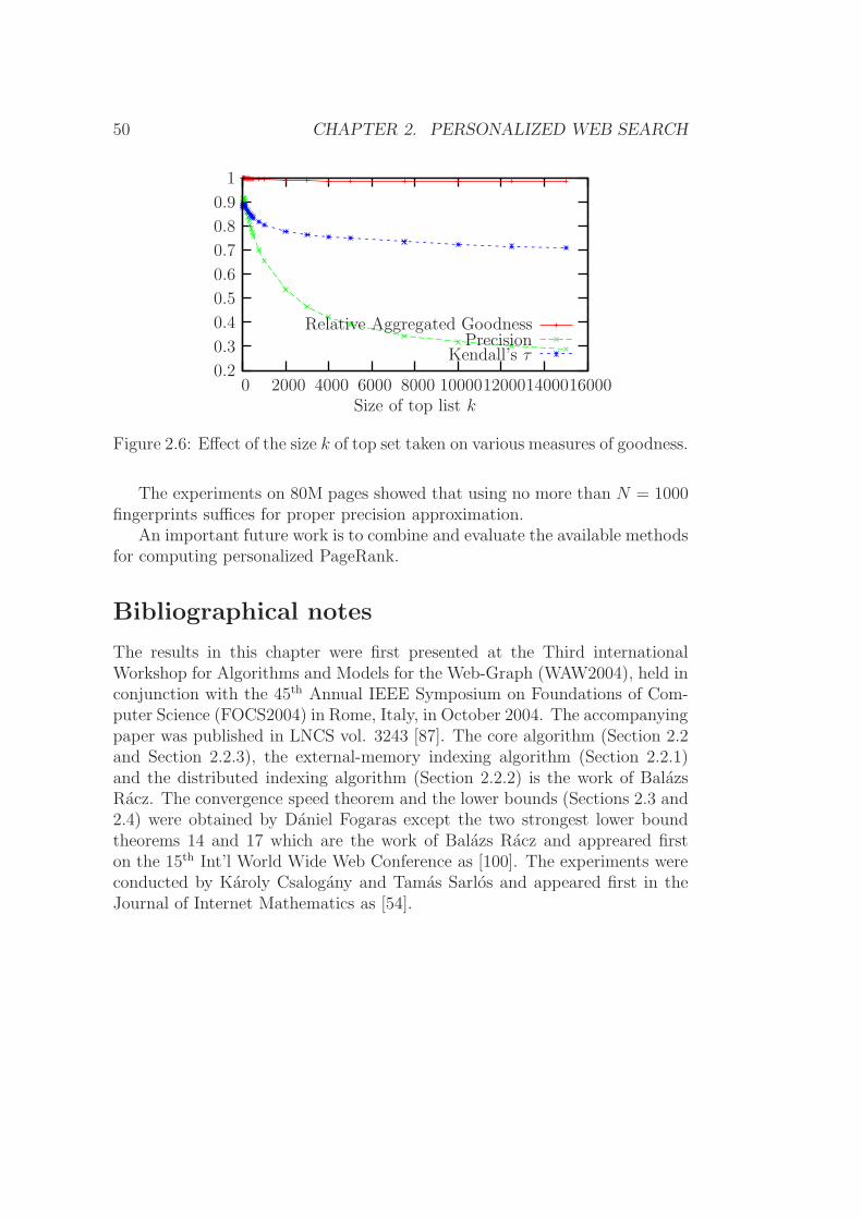
50 CHAPTER 2. PERSONALIZED WEB SEARCH
Kendall’s τPrecision
Relative Aggregated Goodness
Size of top list k1600014000120001000080006000400020000
1
0.9
0.8
0.7
0.6
0.5
0.4
0.3
0.2
Figure 2.6: Effect of the size k of top set taken on various measures of goodness.
The experiments on 80M pages showed that using no more than N = 1000fingerprints suffices for proper precision approximation.
An important future work is to combine and evaluate the available methodsfor computing personalized PageRank.
Bibliographical notes
The results in this chapter were first presented at the Third internationalWorkshop for Algorithms and Models for the Web-Graph (WAW2004), held inconjunction with the 45th Annual IEEE Symposium on Foundations of Com-puter Science (FOCS2004) in Rome, Italy, in October 2004. The accompanyingpaper was published in LNCS vol. 3243 [87]. The core algorithm (Section 2.2and Section 2.2.3), the external-memory indexing algorithm (Section 2.2.1)and the distributed indexing algorithm (Section 2.2.2) is the work of BalazsRacz. The convergence speed theorem and the lower bounds (Sections 2.3 and2.4) were obtained by Daniel Fogaras except the two strongest lower boundtheorems 14 and 17 which are the work of Balazs Racz and appreared firston the 15th Int’l World Wide Web Conference as [100]. The experiments wereconducted by Karoly Csalogany and Tamas Sarlos and appeared first in theJournal of Internet Mathematics as [54].
Chapter 3Similarity Search
3.1 Introduction
The development of similarity search algorithms between web pages is moti-vated by the “related pages” queries of web search engines and web documentclassification. Both applications require efficient evaluation of an underlyingsimilarity function, which extracts similarities from either the textual contentof pages or the hyperlink structure. This chapter focuses on computing sim-ilarities solely from the hyperlink structure modeled by the web graph, withvertices corresponding to web pages and directed arcs to the hyperlinks be-tween pages. In contrast to textual content, link structure is a more homo-geneous and language independent source of information and it is in generalmore resistant against spamming. The authors believe that complex link-basedsimilarity functions with scalable implementations can play such an importantrole in similarity search as PageRank [95] does for query result ranking.
Several link-based similarity functions have been suggested over the webgraph. Functions introduced in social network analysis, like co-citation, bib-liographic coupling, amsler and Jaccard coefficient of neighbors utilize onlythe one-step neighborhoods of pages. To exploit the information in multi-stepneighborhoods, SimRank [74] and the Companion [38] algorithms were intro-duced by adapting the link-based ranking schemes PageRank [95] and HITS[82]. Further methods arise from graph theory such as similarity search basedon network flows [90]. We refer to [89] containing an exhaustive list of link-based similarity search methods.
Unfortunately, no scalable algorithm has so far been published that allowsthe computation of multi-step similarity scores in case of a graph with billionsof vertices. First, all the above algorithms require random access to the webgraph, which does not fit into main memory with standard graph representa-tions. In addition, SimRank iterations update and store a quadratic numberof variables: [74] reports experiments on graphs with less than 300K vertices.Finally, related page queries submitted by users need to be served in less than
51

52 CHAPTER 3. SIMILARITY SEARCH
a second, which has not yet been achieved by any published algorithm.In this chapter we give the first scalable algorithms that can be used to
evaluate multi-step link-based similarity functions over billions of pages on adistributed architecture. With a single machine, we conducted experiments ona test graph of 80M pages. Our primary focus is SimRank, which recursivelyrefines the cocitation measure analogously to how PageRank refines in-degreeranking [95]. In addition we give an improved SimRank variant referred to asPSimRank, which refines the Jaccard coefficient of the in-neighbors of pages.
All our methods are Monte Carlo approximations: we precompute inde-pendent sets of fingerprints for the vertices, such that the similarities can beapproximated from the fingerprints at query time. We only approximate theexact values; fortunately, the precision of approximation can be easily increasedon a distributed architecture by precomputing independent sets of fingerprintsand querying them in parallel.
Besides the algorithmic results we prove several worst case lower boundson the database size of exact and approximate similarity search algorithms.The quadratic lower bound of the exact computation shows the non-existenceof a general algorithm scalable on arbitrary graphs. The results suggest thatscalability can only be achieved either by utilizing some specific property ofthe webgraph or by relaxing the exact computation with approximate methodsas in our case.
We started to investigate the scalability of SimRank in [51], and we gave aMonte Carlo algorithm with the naive representation as outlined in the begin-ning of Section 3.2. The main contributions of this chapter are summarized asfollows:
• In Section 3.2.1 we present a scalable algorithm to compute approximateSimRank scores by using a database of fingerprint trees, an efficientrepresentation of precomputed random walks.
• In Section 3.2.2 we introduce and analyze PSimRank, a novel variant ofSimRank with better theoretical properties and a scalable algorithm.
• In Section 3.3 we show that all the proposed Monte Carlo similaritysearch algorithms are especially suitable for distributed computing.
• In Section 3.4 we prove that our Monte Carlo similarity search algo-rithms approximate the similarity scores with a precision that tends toone exponentially with the number of fingerprints.
• In Section 3.5 we prove quadratic worst case lower bounds on the data-base size of exact similarity search algorithms and linear bounds in caseof randomized approximation computation. The quadratic bounds showthat exact algorithms are not scalable in general, while the linear boundsshow that our algorithms are almost asymptotically worst case space-optimal.

3.1. INTRODUCTION 53
• In Section 3.6 we report experiments about the quality and performanceof the proposed methods evaluated on the Stanford WebBase graph of80M vertices [71].
In the remainder of the introduction we discuss related results, define “scal-ability,” and recall some basic facts about SimRank.
3.1.1 Related Results
Unfortunately the algorithmic details of “related pages” queries in commercialweb search engines are not publicly available. We believe that an accuratesimilarity search algorithm should exploit both the hyperlink structure andthe textual content. For example, the pure link-based algorithms like SimRankcan be integrated with classical text-based information retrieval tools [6] bysimply combining the similarity scores. A very promising text-based methodis when the similarities are extracted from the anchor texts referring to pagesas proposed by [27, 65].
Recent years have witnessed a growing interest in the scalability issue oflink-analysis algorithms. Palmer et al. [96] formulated essentially the samescalability requirements that we will present in Section 3.1.2; they give a scal-able algorithm to estimate the neighborhood functions of vertices. Analogousgoals were achieved by the development of PageRank: Brin and Page [95]introduced PageRank algorithm using main memory of size proportional tothe number of vertices. Then external memory extensions were publishedin [30, 62]. A large amount of research was done to attain scalability for per-sonalized PageRank [66, 54]. The scalability of SimRank was also addressedby pruning [74], but this technique could only scale up to a graph with 300Kvertices in the experiments of [74]. In addition, no theoretical argument waspublished about the error of approximating SimRank scores by pruning. Incontrast, the algorithms of Section 3.2 were used to compute SimRank scoreson a test graph of 80M vertices, and the theorems of Section 3.4 give boundson the error of the approximation.
The key idea of achieving scalability by Monte Carlo (MC) algorithms wasinspired by the seminal papers of Broder et al. [22] and Cohen [31] estimatingthe resemblance of text documents and size of transitive closure of graphs,respectively. Both papers utilize min-hashing, the fingerprinting technique forthe Jaccard coefficient that was also applied in [65] to scale similarity searchbased on anchor text. Our framework of MC similarity search algorithmspresented and analyzed in Section 3.4 is also related to the notion of locality-sensitive hashing (LSH) introduced in [73]. Notice the difference that LSHaggregates 0-1 similarities by testing the equality of hash values (or finger-prints), while our methods aggregate estimated scores from the range [0,1].MC algorithms with simulated random walks also play an important role ina different aspect of web algorithms, when a crawler attempts to downloada uniform sample of web pages and compute various statistics [70, 97, 11] or

54 CHAPTER 3. SIMILARITY SEARCH
page decay [12]. A different approach to achieve scalability by forming clustersof objects and performing lookup only in the query-related cluster appears in[109].
Analogous results to the lower bounds of Section 3.5 are presented in [54]about personalized PageRank problem. Our theorems are proved by the tech-niques of Henzinger et al. [69] showing lower bounds for the space complexitiesof several graph algorithms with stream access to the edges. We refer to thePhD thesis of Bar-Yossef [9] as a comprehensive survey of this field.
3.1.2 Scalability Requirements
In our framework similarity search algorithms serve two types of queries: theoutput of a sim(u, v) similarity query is the similarity score of the given pagesu and v; the output of a relatedα(u) related query is the set of pages for whichthe similarity score with the queried page u is larger than the threshold α.To serve queries efficiently we allow off-line precomputation, so the scalabilityrequirements are formulated in the indexing-query model : we precompute anindex database for a given web graph off-line, and later respond to querieson-line by accessing the database.
We say that a similarity search algorithm is scalable if the following prop-erties hold:
• Time: The index database is precomputed within the time of a sortingoperation, up to a constant factor. To serve a query the index databasecan only be accessed a constant number of times.
• Memory: The algorithms run in external memory : the available mainmemory is constant, so it can be arbitrarily smaller than the size of theweb graph.
• Parallelization: Both precomputation and queries can be implementedto utilize the computing power and storage capacity of thousands ofservers interconnected with a fast local network.
Observe that the time constraint implies that the index database cannotbe too large. In fact our databases will be linear in the number V of vertices(pages). memory requirements do not allow random access to the web graph.We will first sort the edges by their ending vertices using external memorysorting. Later we will read the entire set of edges sequentially as a stream, andrepeat this process a constant number of times.
3.1.3 Preliminaries about SimRank
SimRank was introduced by Jeh and Widom [74] to formalize the intuitionthat
“two pages are similar if they are referenced by similar pages.”

3.1. INTRODUCTION 55
The recursive SimRank iteration propagates similarity scores with a constantdecay factor c ∈ (0, 1), with ℓ indexing the iteration:
simℓ+1(u, v) =c
|I(u)| · |I(v)|∑
u′∈I(u)
∑
v′∈I(v)
simℓ(u′, v′) ,
for vertices u 6= v, where I(x) denotes the set of vertices linking to x; if I(u)or I(v) is empty, then simℓ+1(u, v) = 0 by definition. For a vertex pair withu = v we simply let simℓ+1(u, v) = 1. The SimRank iteration starts withsim0(u, v) = 1 for u = v and sim0(u, v) = 0 otherwise. The SimRank scoreis defined as the limit limℓ→∞ simℓ(u, v); see [74] for the proof of convergence.Throughout this chapter we refer to simℓ(u, v) as a SimRank score, and regardℓ as a parameter.
The SimRank algorithm of [74] calculates the scores by iterating over allpairs of web pages, thus each iteration requires Θ(V 2) time and memory, whereV denotes the number of pages. Thus the algorithm does not meet the scal-ability requirements by its quadratic running time and random access to theweb graph.
We recall two generalizations of SimRank from [74], as we will exploit theseresults frequently. SimRank framework refers to the natural generalization thatreplaces the average function in SimRank iteration by an arbitrary functionof the similarity scores of pairs of in-neighbors. Obviously, the convergencedoes not hold for all the algorithms in the framework, but still simℓ is a well-defined similarity ranking. Several variants are introduced in [74] for differentpurposes.
For the second generalization of SimRank, suppose that a random walkstarts from each vertex and follows the links backwards. Let τu,v denote thefirst meeting time random variable of the walks starting from u and v; τu,v = ∞,if they never meet; and τu,v = 0, if u = v. In addition, let f be an arbitraryfunction that maps the meeting times 0, 1, . . . ,∞ to similarity scores.
Definition 18. The expected f -meeting distance for vertices u and v is de-fined as E(f(τu,v)).
The above definition is adapted from [74] apart from the generalizationthat we do not assume uniform, independent walks of infinite length. In ourcase the walks may be pairwise independent, correlated, finite or infinite. Forexample, we will introduce PSimRank as an expected f -meeting distance ofpairwise coupled random walks in Section 3.2.2.
The following theorem justifies the expected f -meeting distance as a gener-alization of SimRank, formulating it as the expected f -meeting distance withuniform independent walks and f(t) = ct, where c denotes the decay factor ofSimRank with 0 < c < 1. The theorem was proved for infinite ℓ and totallyindependent set of walks in [74]; here we prove a stronger statement.
Theorem 19. For uniform, pairwise independent set of reversed random walksof length ℓ, the equality E(cτu,v) = simℓ(u, v) holds, whether ℓ is finite or not.

56 CHAPTER 3. SIMILARITY SEARCH
Proof. For a fixed graph we proceed by induction on ℓ. Then, the ℓ = ∞ case
follows from limℓ→∞ simℓ(u, v) = sim∞(u, v) and limℓ→∞E(cτℓ
u,v
)= E (
cτ∞
u,v).
The ℓ = 0 case is trivial, and the only non-trivial part is the induction step,when u 6= v and I(u), I(v) 6= ∅ hold. Let us denote by stepx(x
′) the event thatthe reversed walk starting from x proceeds to x′. By applying the pairwiseindependence and the linearity of expectations, we obtain:E(
cτℓ+1u,v
)=
=∑
u′∈I(u)
∑
v′∈I(v)
Pr stepu(u′) and stepv(v
′)
·E(cτℓ+1
u,v | stepu(u′) and stepv(v
′))
=∑
u′∈I(u)
∑
v′∈I(v)
Pr stepu(u′) · Pr stepv(v
′)
·c ·E(cτℓu′,v′
)
=c
|I(u)| · |I(v)|∑
u′∈I(u)
∑
v′∈I(v)
simℓ(u, v)
= simℓ+1(u, v).
3.2 Monte Carlo similarity search algorithms
In this section we give the first scalable algorithm to approximate SimRankscores. In addition, we introduce a new similarity function PSimRank accom-panied by a scalable algorithm.
All the algorithms fit into the framework of Monte Carlo similarity searchalgorithms that will be introduced through the example of SimRank. The-orem 19 expressed SimRank as the expected value simℓ(u, v) = E(cτu,v) forvertices u, v. Our algorithms generate reversed random walks, calculate thefirst meeting time τu,v and estimate simℓ(u, v) by cτu,v . To improve the precisionof approximation, the sampling process is repeated N times and the indepen-dent samples are averaged. The computation is shared between indexing andquerying as shown in Algorithm 3.2.1, a naive implementation. During theprecomputation phase we generate and store N independent reversed randomwalks of length ℓ for each vertex, and the first meeting time τu,v is calcu-lated at query time by reading the random walks from the precomputed indexdatabase.
The main concept of Monte Carlo similarity search already arises in thisexample. In general fingerprint refers to a random object (a random walk in theexample of SimRank) associated with a node in such a way, that the expectedsimilarity of a pair of fingerprints is the similarity of their nodes. The Monte

3.2. MONTE CARLO SIMILARITY SEARCH ALGORITHMS 57
Algorithm 3.2.1 Indexing (naive method) and similarity query
N=number of fingerprints, ℓ=path length, c=decay factor. Indexing: Usesrandom access to the graph.
1: for i := 1 to N do2: for every vertex j of the web graph do3: Fingerprint[i][j][]:=random reversed path of
length ℓ starting from j.
Query sim(u,v):
1: sim:=02: for i := 1 to N do3: Let k be the smallest offset with
Fingerprint[i][u][k]=Fingerprint[i][v][k]4: if such k exists then5: sim:=sim+ck
6: return sim/N
Carlo method precomputes and stores fingerprints in an index database andestimates similarity scores at query time by averaging. The main difficultiesof this framework are as follows:
• During indexing (generating the fingerprints) we have to meet the scala-bility requirements of Section 3.1.2. For example, generating the randomwalks with the naive indexing algorithm requires random access to theweb graph, thus we need to store all the links in main memory. To avoidthis, we will first introduce algorithms utilizing Θ(V ) main memory andthen algorithms using memory of constant size, where V denotes thenumber of vertices. These computational requirements are referred toas semi-external memory [1] and external memory models, respectively.The parallelization techniques will be discussed in Section 3.3.
• To achieve a reasonably sized index database, we need a compact rep-resentation of the fingerprints. In the case of the previous example, theindex database (including an inverted index for related queries) is of size2 ·V ·N · ℓ. In practical examples we have V ≈ 109 vertices and N = 100fingerprints of length ℓ = 10, thus the database is in total 8000 giga-bytes. We will show a compact representation that allows us to encodethe fingerprints in 2 · V · N cells, resulting in an index database of size800 gigabytes.
• We need efficient algorithms for evaluating queries. For queries the mainidea is that the similarity matrix is sparse, for a page u there are relativelyfew other pages that have non-negligible similarity to u. Our algorithmswill enumerate these pages in time proportional to their number.

58 CHAPTER 3. SIMILARITY SEARCH
4
3
31
u5
u4u5 u3
u2
u1
u1
u4
u2
u3
Figure 3.1: Representing the first meeting times of coalescing reversed walksof u1, u2, u3, u4 and u5 (top) with a fingerprint graph (bottom). To decodethe meeting time of u2 and u5: take the paths from u2 and u5 on the bottom.They meet first at u1. The last edges before the meeting have labels 3 and 4.Thus τu2,u5 = max3, 4 = 4.
3.2.1 SimRank
The main idea of this section is that we do not generate totally independentsets of reversed random walks as in Algorithm 3.2.1. Instead, we generate aset of coalescing walks: each pair of walks will follow the same path after theirfirst meeting time. (This coupling is commonly used in the theory of randomwalks.) More precisely, we start a reversed walk from each vertex. In eachtime step, the walks at different vertices step independently to an in-neighborchosen uniformly. If two walks are at the same vertex, they follow the sameedge.
Notice that we can still estimate simℓ(u, v) = E(cτu,v) from the first meetingtime τu,v of coalescing walks, since any pair of walks are independent until theyfirst meet. We will show that the meeting times of coalescing walks can berepresented in a surprisingly compact way by storing only one integer for eachvertex instead of storing walks of length ℓ. In addition, coalescing walks can begenerated more efficiently by the algorithm discussed in Section 3.2.1.3 thantotally independent walks.
3.2.1.1 Fingerprint trees
A set of coalescing reversed random walks can be represented in a compactand efficient way. The main idea is that we do not need to reconstruct theactual paths as long as we can reconstruct the first meeting times for each pairof them. To encode this, we define the fingerprint graph (FPG) for a given setof coalescing random walks as follows.
The vertices of FPG correspond to the vertices of the web graph indexedby 1, 2, . . . , V . For each vertex u, we add a directed edge (u, v) to the FPG forat most one vertex v with
(1) v < u and the fingerprints of u and v first meet at time τu,v < ∞;

3.2. MONTE CARLO SIMILARITY SEARCH ALGORITHMS 59
(2) among vertices satisfying (1) vertex v has earliest meeting time τu,v;
(3) given (1-2), the index of v is minimal.
We label the edge (u, v) with τu,v. An example for a fingerprint graph is shownas Fig. 3.1.
The most important property of the compact FPG representation that itstill allows us to reconstruct τu,v values with the following formula. For a pairof nodes u and v consider the unique paths in the FPG starting from u andv. If these paths have no vertex in common, then τu,v = ∞. Otherwise takethe paths until the first common node w; let t1 and t2 denote the labels ofthe edges on the paths pointing to w; and let t1 = 0 (or t2 = 0), if u = w(or v = w). Then τu,v = maxt1, t2. (See the example of Fig. 3.1.) Thecorrectness of this formula is stated in the lemma below.
Another important property appears in the lemma: each FPG is a collec-tion of rooted trees, which will be referred to as fingerprint trees. The mainobservation for storage and query is that the partition of nodes into fingerprinttrees preserves the locality of the similarity function.
Lemma 20. Consider the fingerprint graph for a set of coalescing randomwalks. This graph is a directed acyclic graph, each node has out-degree at most1, thus it is a forest of rooted trees with edges directed towards the roots.
Consider the unique path in the fingerprint graph starting from vertex u.The indices of nodes it visits are strictly decreasing, and the labels on the edgesare strictly increasing.
Any first meeting time τu,v can be determined by τu,v = maxt1, t2 asdetailed above.
Proof. The first two statements naturally follow from the definition of finger-print graphs, so we focus on the last statement. Notice that τu,v < ∞ iff P (u)and P (v) has a common vertex, where P (x) denotes the unique path in theFPG starting from vertex x. This naturally follows from the transitivity ofrelation (u, v) : τu,v < ∞. Thus, it remains to prove that τu,v = maxt1, t2holds for any vertices u, v with τu,v < ∞.
Let us denote by w the first common vertex of paths P (u) and P (v). Forx = u, v let |P (x, w)| be the number of edges in P (x) from x to w; and if|P (x, w)| > 0, let x′ denote the first vertex of P (x) following x. We will referto the labels of (u, u′) and (v, v′) as t′1 and t′2. Recall that t1 and t2 denotethe labels of the edges of P (u) and P (v) with ending vertex w; furthermoret1 = 0 (or t2 = 0) if |P (u, w)| = 0 (or |P (v, w)| = 0). We refer to Fig. 3.2summarizing the notation.
We will proceed induction on k = |P (u, w)|+ |P (v, w)| to prove that τu,v =maxt1, t2 holds for any vertices u, v with τu,v < ∞. The k = 1 case is trivial,and the induction step from k to k + 1 will be proved from the following factreferred to as the generalized transitivity :
∞ > τu,v ≥ τv,z =⇒ τu,v = τu,z.

60 CHAPTER 3. SIMILARITY SEARCH
t′2
wt1
t2v′
u′
v
u t′1
Figure 3.2: Notation of specific vertices and edge labels of a fingerprint graph.In the example |P (u, w)| = 3 and |P (v, w)| = 4.
We first discuss the case when one of u, v equals w, we may assume wlogthat u = w and v 6= w. By the definition of FPG w = u < v, so τu,v ≥ t′2 =τv,v′ . From the generalized transitivity we get τu,v = τu,v′ , which is equal tomaxt1, t2 = t2 by induction.
In case of u 6= w and v 6= w assume (wlog) that t′2 ≤ t′1. If u < v, thenτu,v ≥ t′2 = τv,v′ . If u > v, then τu,v ≥ t′1 ≥ t′2 = τv,v′ . In both subcases weconclude that τu,v ≥ τv,v′ , so we get τu,v = τu,v′ by the generalized transitivity.By induction τu,v = τu,v′ = maxt1, t2, if v′ 6= w; otherwise τu,v = τu,v′ =maxt1, 0 = maxt1, t2, the last equality following from t1 ≥ t′1 ≥ t′2 =t2.
3.2.1.2 Fingerprint database and query processing
The first advantage of the fingerprint graph (FPG) is that it represents all firstmeeting times for a set of coalescing walks of length ℓ in compact manner. Itis compact, since every vertex has at most one out-edge in an FPG, so thesize of one graph is V , and N · V bounds the total size.1 This is a significantimprovement over the naive representation of the walks with a size of N ·V · ℓ.
The second important property of the FPG is that two vertices have non-zero estimated similarity iff they fall into the same fingerprint tree (same com-ponent of the FPG). Thus, when serving a related(u) query it is enough toread and traverse from each of the N fingerprint graphs the unique tree con-taining u. Therefore in a fingerprint database, we store the fingerprint graphsordered as a collection of fingerprint trees, and for each vertex u we also storethe identifiers of the N trees containing u. By adding the identifiers the totalsize of the database is no more than 2 · N · V .
A related(u) query requires N + 1 accesses to the fingerprint database:one for the tree identifiers and then N more for the fingerprint trees of u.A sim(u, v) query accesses the fingerprint database at most N + 2 times, byloading two lists of identifiers and then the trees containing both u and v. Forboth type of queries the trees can be traversed in time linear in the size of thetree.
Notice that the query algorithms do not meet all the scalability require-ments: although the number of database accesses is constant (at most N+2),the memory requirement for storing and traversing one fingerprint tree may
1To be more precise we need V (⌈log(V )⌉ + ⌈log(ℓ)⌉) bits for an FPG to store the labeled edges. Noticethat the weights require no more than ⌈log(ℓ)⌉ = 4 bits for each vertex for typical value of ℓ = 10.

3.2. MONTE CARLO SIMILARITY SEARCH ALGORITHMS 61
be as large as the number of pages V . Thus, theoretically the algorithm mayuse as much as V memory.
Fortunately, in case of web data the algorithm performs as an externalmemory algorithm. As verified by our numerical experiments on 80M pages(see in Section 3.6.3) the average sizes of fingerprint trees are approximately100–200 for reasonable path lengths. Even the largest trees in our databasehad at most 10K–20K vertices, thus 50Kbytes of data needs to be read foreach database access in worst case.
3.2.1.3 Building the fingerprint database
It remains to present a scalable algorithm to generate coalescing sets of walksand compute the fingerprint graphs.
As opposed to the naive algorithm generating the fingerprints one-by-one,we generate all fingerprints together. With one iteration we extend all partiallygenerated fingerprints by one edge. To achieve this, we generate one uniformin-edge ej for each vertex j independently. Then extend with edge ej each ofthose fingerprints that have the same last node j. This method generates acoalescing set of walks, since a pair of walks will be extended with the sameedge after they first meet. Furthermore, they are independent until the firstmeeting time.
The pseudo-code is displayed as Algorithm 3.2.2, where NextIn[j] stores thestarting vertex of the randomly chosen edge ej, and PathEnd[j] is the endingvertex of the partial fingerprint that started from j. To be more precise, ifa group of walks already met, then PathEnd[j]=“stopped” for every memberj of the group except for the smallest j. The SaveNewFPGEdges subroutinedetects if a group of walks meets in the current iteration, saves the fingerprinttree edges corresponding to the meetings and sets PathEnd[j]=“stopped” forall non-minimal members j of the group. This can be accomplished by a lineartime counting sort of the non-stopped elements of PathEnd array.
The subroutine GenRndInEdges may generate a set of random in-edges witha simple external memory algorithm if the edges are sorted by the endingvertices. A significant improvement can be achieved by generating all therequired random edge-sets together during a single scan over the edges of thegraph. Thus, all the N · ℓ edge-scans can be replaced by one edge-scan savingmany sets of in-edges. Then GenRndInEdges sequentially reads the N · ℓ arraysof size V from disk.
The algorithm outlined above fits into the semi-external memory model,since it utilizes 2·V main memory to store the PathEnd and NextIn arrays. (Thecounter sort operation of SaveNewFPGEdges may reuse NextIn array, so it doesnot require additional storage capacity.) The algorithm can be easily convertedinto the external memory model by keeping PathEnd and NextIn arrays on thedisk and by replacing Lines 6-8 of Algorithm 3.2.2 with external sorting andmerging processes. Furthermore, at the end of the indexing the individualfingerprint trees can be collected with ℓ sorting and merging operations, as the

62 CHAPTER 3. SIMILARITY SEARCH
Algorithm 3.2.2 Indexing (using 2 · V main memory)
N=number of fingerprints, ℓ=length of paths. Uses subroutine GenRndInEdges
that generates a random in-edge for each vertex in the graph and stores itssource in an array.
1: for i := 1 to N do2: for every vertex j of the web graph do3: PathEnd[j] := j /*start a path from j*/4: for k:=1 to ℓ do5: NextIn[] := GenRndInEdges();6: for every vertex j with PathEnd[j]6=“stopped” do7: PathEnd[j]:=NextIn[PathEnd[j]] /*extend the path*/8: SaveNewFPGEdges(PathEnd)9: Collect edges into trees and save as FPGi.
longest possible path in each fingerprint tree is ℓ (due to Lemma 20 the labelsare strictly increasing but cannot grow over ℓ).
3.2.2 PSimRank
In this section we give a new SimRank variant with properties extending thoseof Minimax SimRank [74], a non-scalable algorithm that cannot be formulatedin our framework. The new similarity function will be expressed as an expectedf -meeting distance by modifying the distribution of the set of random walksand by keeping f(t) = ct.
A deficiency of SimRank can be best viewed by an example. Consider twovery popular web portals. Many users link to both pages on their personalwebsites, but these pages are not reported to be similar by SimRank. Anextreme case is when nodes u and v have the same in-neighborhood of size k,which have no in-edges. Though the k pages are totally dissimilar in the link-based sense, we would still intuitively regard u and v as similar. UnfortunatelySimRank is counter-intuitive in this case, as simℓ(u, v) = c · 1
ktends to zero as
the number k of common in-neighbors increases.
3.2.2.1 Coupled random walks
We solve the deficiency of SimRank by allowing the random walks to meet withhigher probability when they are close to each other: a pair of random walksat vertices u′, v′ will advance to the same vertex (i.e., meet in one step) with
probability of the Jaccard coefficient |I(u′)∩I(v′)||I(u′)∪I(v′)|
of their in-neighborhoods I(u′)
and I(v′). Thus these walks will be coupled as opposed to the independentwalks of SimRank.
Definition 21. PSimRank is the expected f -meeting distance with f(t) = ct
(for some 0 < c < 1) of the following set of random walks. For each vertex u,

3.2. MONTE CARLO SIMILARITY SEARCH ALGORITHMS 63
the random walk Xu makes ℓ uniform independent steps on the transposed webgraph starting from point u. For each pair of vertices u, v and time t, assumethat the random walks are at position Xu(t) = u′ and Xv(t) = v′. Then
• with probability |I(u′)∩I(v′)||I(u′)∪I(v′)|
they both step to the same uniformly chosen
vertex of I(u′) ∩ I(v′);
• with probability |I(u′)\I(v′)||I(u′)∪I(v′)|
the walk Xu steps to a uniform vertex in I(u′)\I(v′) and the walk Xv steps to an independently chosen uniform vertexin I(v′);
• with probability |I(v′)\I(u′)||I(u′)∪I(v′)|
the walk Xv steps to a uniform vertex in I(v′)\I(u′) and the walk Xu steps to an independently chosen uniform vertexin I(u′).
We give a set of random walks satisfying the coupling of the definition.For each time t ≥ 0 we choose an independent random permutation σt on thevertices of the web graph. At time t if the random walk from vertex u is atXu(t) = u′, it will step to the in-neighbor with smallest index given by thepermutation σt, i.e.,
Xu(t + 1) = argminu′′∈I(u′)
σt(u′′)
It is easy to see that the random walk Xu takes uniform independent steps,since we have a new permutation for each step. The above coupling is alsosatisfied, since for any pair u′, v′ the vertex argminw∈I(u′)∪I(v′) σt(w) falls intothe sets I(u′) ∩ I(v′), I(u′) \ I(v′), I(v′) \ I(u′) with probabilities
|I(u′) ∩ I(v′)||I(u′) ∪ I(v′)| ,
|I(u′) \ I(v′)||I(u′) ∪ I(v′)| and
|I(v′) \ I(u′)||I(u′) ∪ I(v′)| , resp.
PSimRank can be computed by the following linear equation system, plac-ing PSimRank in the SimRank framework, which also proves that the valuesdo not depend on the actual choice of the coupling:
psimℓ+1(u, v) = 1, if u = v;psimℓ+1(u, v) = 0, if I(u) = ∅ or I(v) = ∅;psimℓ+1(u, v) = c ·
[|I(u)∩I(v)||I(u)∪I(v)|
· 1+
+ |I(u)\I(v)||I(u)∪I(v)|
· 1|I(u)\I(v)||I(v)|
∑u′∈I(u)\I(v)
v′∈I(v)
psimℓ(u′, v′)+
+ |I(v)\I(u)||I(u)∪I(v)|
· 1|I(v)\I(u)||I(u)|
∑v′∈I(v)\I(u)
u′∈I(u)
psimℓ(u′, v′)
].

64 CHAPTER 3. SIMILARITY SEARCH
3.2.2.2 Computing PSimRank
To achieve a scalable algorithm for PSimRank we modify the SimRank in-dexing and query algorithms introduced in Section 3.2.1. The following resultallows us to use the compact representation of fingerprint graphs.
Lemma 22. Any set of random walks satisfying the PSimRank requirementsare coalescing, i.e., any pair follows the same path after their first meetingtime.
Proof. Let u and v be arbitrary nodes. By the first coupling requirement, ifat time t the random walks Xu and Xv are at the same nodes u′ = v′, thenI(u′) = I(v′), thus with probability |I(u′)∩I(v′)|
|I(u′)∪I(v′)= 1 they proceed to the same
vertex.
To apply the indexing algorithm of SimRank, we only need to ensure thepairwise coupling. This can be accomplished by replacing the GenRndInEdges
procedure, which generated one independent, uniform in-edge for each vertex vin the graph for SimRank. In case of PSimRank, GenRndInEdges chooses a per-mutation σ at random; and then for each vertex v the in-neighbor with small-est index under the permutation σ is selected, i.e., vertex argminv′∈I(v) σ(v′) ischosen.
As in the case of the GenRndInEdges for SimRank, all required sets of randomin-edges can be generated within a single scan over the edges of the web graph,if the graph edges are sorted. The random permutations can be stored insmall space by random linear transformations [23], thus the external memoryimplementation of SimRank can be extended to PSimRank.
3.2.3 Updating the index database
The web graph is not static, it changes over time quite rapidly. Web searchengines are required to maintain a fairly up-to-date index database and areconstantly refreshing the pages they have indexed. As a consequence, the webgraph from which we compute our similarity scores is also changing: nodes andedges are added and removed constantly. In this section we describe possibili-ties to maintain an up-to-date index database in this chaning environment.
Brute force updating
In general purpose web search engines it is not common to have daily updatesof the entire index database. Furthermore, there is a huge difference in work-load between peak and off-peak periods, which means that considerable idleresources can be assigned for reindexing. The advantage of our method is thatnot all the N independent fingerprints are required to be recomputed at thesame time, it can be distributed among multiple idle periods and multiple ma-chines. In case of specialized news or blogosphere search engines the amount

3.2. MONTE CARLO SIMILARITY SEARCH ALGORITHMS 65
of data is considerably less, thus less resources are required for rebuilding theindex.
Incorporating slight changes
Assume only a single node u has changed. If we don’t use the compression givenby the Fingerprint Graph representation, but build the index by the fingerprintpaths, then the respective inverted index required for the queries has the listof the paths going through node u. These paths have to be examined forpossible change. If the original degree was k and one link was added then withprobability k
k+1the database is not to be modified, with probability 1
k+1the
paths have to be routed through the new link (where they coalesce with otherwalks). Assuming the changes are really slight, a disk-based implementationsuffices.
In case of PSimRank we can incorporate slight changes into the FPG data-base: Given the changed node u and the saved seeds of the random permu-tations, follow the path from the changed point until the end. (This will bedifferent for each of the ℓ possible positions where u might occur on a finger-print path.) Denote the set of these ending vertices by U . As each fingerprinttree contains those nodes’ paths that coalesced in ℓ steps, the ending vertexof the paths in a fingerprint tree is the same. Thus each fingerprint tree hasa unique ending vertex. Select the fingerprint trees that have ending vertexin U (this might require an N · V sized index). Examine them for possiblechange. It can be seen that at most one edge has to be changed in the FPG,but that might attach a subtree to a different fingerprint tree. As there are atmost |U | ≤ ℓ trees to examine, this is feasible for incorporating slight changes.
Indexing based on the previous index
It is a common technique in PageRank index updates to use the solutionof the previous database as a starting point for the new iteration. We canuse this approach to gain a very interesting algorithm for index update thatworks on the FPG database for both SimRank and PSimRank. Performing asingle iteration decays the current database and the expected solution’s norm-distance by a factor of c. As we can have relatively small c (see Fig. 3.4), alarge effect of incorporating the graph changes into the index can be achievedby a single iteration.
A single iteration of the linear system starting from the previous solutionis represented in the fingerprint model by prepending a random edge to allfingerprints. This can be accomplished as follows: Run GenRndInEdges. Sortthe result according to the generated in-neighbors’ fingerprint trees. Then foreach fingerprint tree and the new edges which we have to prepend to it, dothe following: Decompress the fingerprint tree into coalescing reverse walksusing unlabeled points as Fig. 3.1 displays. Then prepend the new edges tothe reverse walks (attach them to the labeled points). Remove all paths that

66 CHAPTER 3. SIMILARITY SEARCH
have no edges prepended2, then relabel the nodes according to the new startingpoints. Remove the last step so that ℓ does not change due to the reindexing.The coalesced walks might fall apart into more sets of coalesced walks at thisstep. Finally each of the resulting sets of walks have to be compressed into afingerprint tree.
The very interesting property of this update method is that the changesin the graph are introduced from the MSB (most significant ‘digit’) into theindex. Assuming each night one such iteration is performed, then a new edgewill be fully reflected only after ℓ = 10 days, but the most important changeswill be visible after the first night. Notice that if so desired, then more thanone steps can be prepended to the fingerprint trees with one run of the abovealgorithm having more GenRndInEdges and sorts but a single iteration over theactual database (the fingerprint trees).
3.3 Monte Carlo parallelization
In this section we discuss the parallelization possibilities of our methods. Weshow that all of them exhibit features (such as fault tolerance, load balancingand dynamic adaptation to workload) which makes them extremely applicablein large-scale web search engines.
All similarity methods we have given in this chapter are organized aroundthe same concepts:
• we compute a similarity measure by averaging N independent samplesfrom a random variable;
• the independent samples are stored in N instances of an index database,each capable of producing a sample of the random variable for any pairof vertices.
The above framework allows a straightforward parallelization of both theindexing and the query: the computation of independent index databases canbe performed on up to N different machines. Then the databases are trans-ferred to the backend computers that serve the query requests. When a requestarrives to the frontend server, it asks all (up to N) backend servers, averagestheir answers and returns the results to the user.
The Monte Carlo parallelization scheme has many advantages that makeit perfectly suitable to large-scale web search engines:
Fault tolerance. If one or more backend servers cannot respond to thequery in time, then the frontend can aggregate the results of the remainingones and calculate the estimate from the available answers. This will notinfluence service availability, and results in a slight loss of precision.
2If no paths have edges prepended, then the entire tree has to be dropped.

3.4. ERROR OF APPROXIMATION 67
Load balancing. In case of very high query loads, more than N backendservers (database servers) can be employed. A simple solution is to replicatethe individual index databases. Better results are achieved if one calculates anindependent index database for all the backend servers. In this case it sufficesto ask any N backend servers for a proper precision answer. This allowsseamless load balancing, i.e., you can add more backend servers one-by-one asthe demand increases.
Dynamic adaptation to workload. During times of excessive load the num-ber of backend servers asked for each query (N) can be automatically reducedto maintain fast response times and thus service integrity. Meanwhile, duringidle periods, this value can be increased to get higher precision for free (alongwith better utilization of resources). We believe that this feature is extremelyimportant in the applicability of our results.
3.4 Error of approximation
As we have seen in earlier sections, a crucial parameter of our methods isthe number N of fingerprints. The index database size, indexing time, querytime and database accesses are all linear in N . In this section we formallyanalyze the number of fingerprints needed for a given precision approximation.Our theorems show that even a modest number of fingerprints (e.g., N =100) suffices for the purposes of a web search engine. A further theoreticalconsequence that N can be regarded as a constant, when the precision anderror probability are fixed.
To state our results we need a suitably general model that can accommo-date our methods for SimRank and PSimRank. Suppose that a randomizedalgorithm assigns N independent sets of fingerprints for the vertices and forany two vertices u, v a function maps the fingerprints to a score Si(u, v) ∈ [0, 1]for i = 1, . . . , N such that E(Si(u, v)) = sim(u, v) for some similarity functionsim(·, ·). We will refer to sım(u, v) = 1
N
∑Ni=1 Si(u, v) as a Monte Carlo simi-
larity function, which is a random function with E(sım(u, v)) = sim(u, v) bylinearity. Notice that the approximate scores of our algorithms for SimRankand PSimRank can be regarded as Monte Carlo similarity functions sım(·, ·).
Theorem 23. For any Monte Carlo similarity function sım the absolute errorconverges to zero exponentially in the number of fingerprints N and uniformlyover the pair of vertices u, v. More precisely, for any vertices u, v and anyδ > 0 we have
Pr| sım(u, v) − sim(u, v)| > δ < 2e−67Nδ2
Proof. We shall use Bernstein’s inequality in the following form. For anyindependent, identically distributed random variables Zi : i = 1, 2, . . . , N that

68 CHAPTER 3. SIMILARITY SEARCH
have a bounded range [a, b], for any δ > 0:
Pr| 1
N
N∑
i=1
Zi −EZ| > δ ≤ 2e−N δ2
2 Var Z+2δ(b−a)/3
Applying this for Zi = Si(u, v) and using the bounds Zi ∈ [0, 1], Var Zi ≤ 14,
and δ < 1 the statement follows.
Notice that the bound uniformly applies to all graphs and all Monte Carlosimilarity functions, such as our approximations for SimRank and PSimRank.However, this bound concerns the convergence of the similarity score for onepair of vertices only. In the web search scenario, we typically use relatedqueries, thus are interested in the relative order of pages according to theirsimilarity to a given query page u. The above result implies that for a querypage u the probability of interchanging two result pages v and w in the resultlists tends to zero exponentially:
Corollary 24. There exist constants β1, β2 such that for any Monte Carlo sim-ilarity function sım and pages u, v and w for which δ = sim(u, v)− sim(u, w) >0, the following holds:
Prsım(u, v) < sım(u, w) < β1e−β2Nδ2
These theorems mean that the Monte Carlo approximation can efficientlycapture the big differences among the similarity scores. But in case of smalldifferences, the error of approximation obscures the actual similarity ranking,and an almost arbitrary reordering is possible. We believe, that for a websearch inspired similarity ranking it is sufficient to distinguish between verysimilar, modestly similar, and dissimilar pages. We can formulate this require-ment in terms of a slightly weakened version of classical information retrievalmeasures precision and recall [6].
Consider a related query for page u with similarity threshold α, i.e., theproblem is to return the set of pages S = v : sim(u, v) > α. Our methods
approximate this set with R = v : sım(u, v) > α. We weaken the notionof precision and recall to exclude a small, δ sized interval of similarity scoresaround the threshold α: let R+δ = v : sim(u, v) > α + δ, R−δ = v :sim(u, v) > α − δ. Then the expected δ-recall of a Monte Carlo similarity
function is E(| bR∩R+δ|)
|R+δ|while the expected δ-precision is E(| bR∩R−δ|)E(| bR|)
. We denote
by Rc−δ the complement set of R−δ.
Theorem 25. For any Monte Carlo similarity function sım, any page u, sim-ilarity threshold α and δ > 0 the expected δ-recall is at least 1 − e−
67Nδ2
andthe expected δ-precision is at least
1 − |Rc−δ|
|R+δ|1
e67Nδ2 − 1
.

3.5. LOWER BOUNDS FOR THE SIMILARITY DATABASE SIZE 69
Proof. We only prove the bound for the expected δ-recall, the precision canbe proved with analogous steps.E(
|R ∩ R+δ|)
=
= E( ∑
v∈R+δ
1v ∈ R)
=∑
v∈R+δ
Prv ∈ R
≥∑
v∈R+δ
(1 − e−
67Nδ2
)= |R+δ| ·
(1 − e−
67Nδ2
),
where the second equation follows from the linearity of expectation; and theinequality follows from the one-sided absolute error bound Prsım(u, v) −sim(u, v) < −δ < e−
67Nδ2
that can be proved analogously to Theorem 23.
This theorem shows that the expected δ-recall converges to 1 exponentiallyand uniformly over all possible similarity functions, graphs and queried verticesof the graphs, while the expected δ-precision converges to 1 exponentially forany fixed similarity function, graph and queried node.
3.5 Lower Bounds for the Similarity Database
Size
In this section we will prove several lower bounds on the space complexity ofcalculating SimRank and PSimRank functions. In particular, we prove thatexcept for the approximate approach, the required similarity database sizesare at least Ω(V 2) bits for some graphs with V vertices; which in turn meansthat exact computation is infeasible for large-scale computation. On the otherhand, the lower bound for the approximate problem is linear in V , which ismatched by our algorithm of Section 2.2 up to a logarithmic factor. Notice,that the worst case bounds cannot be applied to one particular input such asthe webgraph. The main consequence of the theorems about similarity searchis that the web-search community should either utilize some specific propertyof the webgraph or relax the exact problem to an approximate one as in ourscenario.
More precisely we will consider two-phase algorithms: in the first phasethe algorithm has access to the edge set of the graph and has to computean index database; in the second phase the algorithm gets a query, and hasto answer based on the index database, i.e., the algorithm cannot access thegraph during query-time. A b(V ) worst case lower bound on the database sizeholds, if for any two-phase algorithm there exists a graph on V vertices suchthat the algorithm builds an index database of b(V ) bits.
In the two-phase model we will consider the below listed types of queries,where sim(·, ·) denotes a similarity function. The input of the queries arevertices u, v (and w), the numbers ǫ and δ are fixed before the indexing phase.

70 CHAPTER 3. SIMILARITY SEARCH
u1 u2 u3 uk
vnvn−1
zkz2 z3
v1 v2 v3 v4
z1
Figure 3.3: Encoding a vector x of m = n · k bits into a graph Gx. Theexistence of a dashed edge indicates that the corresponding bit xy was set toxy = 1.
(1) Exact: given the vertices u, v, calculate sim(u, v).
(2) Approximate: Estimate sim(u, v) with a sım(u, v) such that for fixed ǫ, δ >0
Pr| sım(u, v) − sim(u, v)| < δ ≥ 1 − ǫ
(3) Positivity: Decide whether sim(u, v) > 0 holds with error probability atmost ǫ.
(4) Comparison: given the vertices u, v, w, decide whether sim(u, v) > sim(u, w)holds with error probability at most ǫ.
(5) ǫ–δ comparison: given the vertices u, v, w with | sim(u, v)− sim(u, w)| > δ,decide whether sim(u, v) > sim(u, w) holds with error probability at mostǫ.
Our tool towards the lower bounds will be the asymmetric communicationcomplexity game bit-vector probing [69]: there are two players A and B; playerA has a vector x of m bits; player B has a number y ∈ 1, 2, . . . , m; and theyhave to compute the function f(x, y) = xy, i.e., the output is the yth bit of theinput vector x. To compute the proper output they have to communicate, andcommunication is restricted in the direction A → B. The one-way communi-cation complexity [84] of this function is the number of transferred bits in theworst case by the best protocol.
Theorem 26 ([69]). Any protocol that outputs the correct answer to the bit-vector probing problem with probability at least 1+γ
2must transmit at least γm
bits.
In our theorems, we will substitute the function sim(·, ·) by SimRank andPSimRank with path length ℓ = 1 and we omit the decay factor by settingc = 1−. So sim(u, v) = |I(u)∩I(v)|
|I(u)|·|I(v)|for SimRank and sim(u, v) = |I(u)∩I(v)|
|I(u)∪I(v)|
for PSimRank, where I(w) denotes the in-neighbors of w. We mention thatall results can be easily extended for any constant c and ℓ. The followingconstruction encodes the bits of a vector into the similarity scores of a graph.

3.5. LOWER BOUNDS FOR THE SIMILARITY DATABASE SIZE 71
Construction 27. Suppose that x is a vector of m bits, where m = k · n forsome k ≤ n. Let Gx denote the graph with 2k+n vertices denoted by u1, . . . , uk,z1, . . . , zk, and v1, . . . , vn. For each 1 ≤ i ≤ k and 1 ≤ j ≤ n the edge (zi, vj)is in the graph iff bit (j − 1)k + i is set in the vector x; furthermore, we addan edge (zi, ui) for all 1 ≤ i ≤ k. See Fig. 3.3 for the notation.
It easily follows from the construction that sim(ui, vj) = 1|I(vj)|
≥ 1k, if the
bit (j−1)k+i is 1 in the vector x, and sim(ui, vj) = 0 otherwise, where sim(·, ·)denotes either SimRank or PSimRank. Now we are ready to prove our lowerbounds.
Theorem 28. Any algorithm solving the positivity problem (3) of SimRankor PSimRank with probability at least 1+γ
2must use a database of size Ω(γV 2)
bits in worst case.
Proof. The proof is the same for the three similarity functions. We give acommunication protocol for the bit-vector probing problem as follows. Givenan input x of m = n2 bits, Player A creates a graph Gx with the aboveconstruction, where k = n. Then A computes a similarity index database fromGx and transmits the database to Player B. As B wants to know the bit xy, heuses the positivity query algorithm for the vertices ui, vj, where y = (j−1)k+i.By Construction 27 the answer to the query is true iff xy = 1 holds. Thus ifthe two-phase algorithm solves the positivity query with probability 1+γ
2, then
this protocol solves the bit-vector probing problem with probability 1+γ2
, sothe size of the transferred database is at least γm = γn2 = γ(V/3)2.
Corollary 29. Any algorithm solving the exact problem (1) for SimRank orPSimRank must have a similarity database of size Ω(V 2) bits in worst case.
Theorem 30. Any algorithm solving the approximation problem (2) for Sim-Rank or PSimRank needs in worst case an index database of Ω(1−2ǫ
δV ) bits, if
δ = Ω( 1V
); and Ω((1 − 2ǫ)V 2) otherwise.
Proof. The proof is essentially the same as that of Theorem 28 with differentparameters in the construction. Let k = min( 1
2δ+1, V
3) and n = V − 2k. Player
A encodes a vector x of m = n ·k bits into a graph Gx by Construction 27 andtransmits the index database to player B. Recall that either sim(ui, vj) ≥ 1
k
or sim(ui, vj) = 0 depending on the bit y = (j − 1)k + i, so sim(ui, vj) > 2δiff xy = 1. Then Player B decides on xy = 1 iff sım(ui, vj) > δ holds for theapproximate score. The above outlined protocol solves the bit vector probingwith probability 1 − ǫ = 1+γ
2. By Theorem 26 the database size is at least
γm = γkn ≥ (1 − 2ǫ)k · V3, which completes the proof.
This radical drop in the storage complexity is not surprising, as our ap-proximation algorithm achieves this bound up to a logarithmic factor: for afixed ǫ, δ we can calculate the necessary number of fingerprints N by Theo-rem 23 (or by Theorem 24 for the ǫ–δ comparison problem), and then for each

72 CHAPTER 3. SIMILARITY SEARCH
vertex in the graph we store exactly N fingerprints, independently of the sizeof the graph. This is a linear database, though the constant makes it veryimpractical. In the comparison problems (4) and (5) we have the same results.
Theorem 31. Any algorithm solving the comparison problem (4) for SimRankor PSimRank with probability 1+γ
2requires a similarity database of Ω(γV 2) bits
in worst case.
Proof. We will modify the proof of Theorem 28 by changing the graph con-struction. Player A encodes x into a graph Gx with k = n by Construction 27.Then another set w1, . . . , wn is added to the vertices of Gx such that wj isthe complement of vj : Player A puts an additional arc (zi, wj) in the graphiff (zi, vj) is not an arc, which means that bit (i − 1)n + j was not set in theinput vector.
Then upon quering bit y = (i−1)n+j, exactly one of sim(ui, vj), sim(ui, wj)will be positive (depending on the input bit xy), thus the comparison querysim(ui, vj) > sim(ui, wj) will yield the required output for the bit-vector prob-ing problem.
Corollary 32. Any algorithm solving the ǫ–δ comparison problem (5) for Sim-Rank or PSimRank needs in worst case a similarity database of Ω(1−2ǫ
δV ) bits
on graphs with V = Ω(1δ) vertices, and Ω((1 − 2ǫ)V 2) bits otherwise.
Proof. Modifying the proof of Theorem 31 along the lines of the proof of The-orem 30 yields the necessary results.
3.6 Experiments
This section presents our experiments on the repository of 80M pages crawledby the Stanford WebBase project in 2001. The following problems are ad-dressed by our experiments:
• How do the parameters ℓ, N and c effect the quality of the similaritysearch algorithms? The dependence on path length ℓ shows that multi-step neighborhoods contain more valuable similarity information thansingle-step neighborhoods. Quality increases in each step until ℓ = 5.
• How do the qualities of SimRank and PSimRank relate to each other andto other link-based methods? We conclude that PSimRank outperformsall the other methods.
• What are the average and maximal sizes of fingerprint trees for SimRankand PSimRank? This is important, as the running time and memoryrequirement of query algorithms are proportional to these sizes. Wemeasured sizes as small as 100 − 200 on average implying fast runningtime with low memory requirement.

3.6. EXPERIMENTS 73
• What is the actual query serving performance of our methods? How doesthis performance scale as we add more servers and utilize the Monte Carloparallelization possibilities?
3.6.1 Similarity Score Quality Measures
We briefly summarize the method of Haveliwala et al. [65] to measure thequality of similarity search algorithms; see [65] for a more detailed description.The most imortant property of this method is that it requires no expensiveuser survey. This allows a much greater number of pages to be included inthe measurement (in our case 218,720 pages, as opposed to a typical usersurvey covering ≈1000 pages). Furthermore, the experiment is reproducible,and different parameter settings can be evaluated automatically.
The similarity search algorithms will be compared to a ground truth simi-larity ordering extracted from the Open Directory Project (ODP, [94]) data, ahierarchical collection of webpages managed by thousands of volunteer editors.The ODP category tree implicitly encodes similarity information: view it as anundirected graph and the consider the shortest-path-length function (siblingsare more similar than cousins). Given a uniformly chosen query page u, thispartial order will be compared to the order returned by the algorithm usingthe Kruskal-Goodman Γ measure:
Γ = 2 · Prsım(u, v) > sım(u, w)|sım(u, v) 6= sım(u, w) andsim(u, v) > sim(u, w) − 1
where sım(·, ·) represents the similarity search algorithm to evaluate and sim(·, ·)is the ODP similarity. As u, v, w are uniform random, the condition restrictscomputation to pages in the ODP (218,720 in our case) and to capture the topranked portion of the result lists we further restrict v, w to be chosen from u’ssiblings and cousins in the ODP tree, denoted by sibling Γ [65].
3.6.2 Comparing the Quality under Various Parameter
Settings
All the quality measurements were performed on a web graph of 78,636,371pages crawled and parsed by the Stanford WebBase project in 2001. In ourcopy of the ODP tree 218,720 urls were found falling into 544 classes aftercollapsing the tree at level 3. The indexing process took 4 hours for SimRankand 14 hours for PSimRank with path length ℓ = 10 and N = 100 fingerprints.We ran a semi-external memory implementation on a single machine with2.8GHz Intel Pentium 4 processor, 2GB main memory and Linux OS. Thetotal size of the computed database would have been 68GB. Since sibling Γ isbased on similarity scores between vertices of the ODP pages, we only savedthe fingerprints of the 218,720 ODP pages. A nice property of our methods

74 CHAPTER 3. SIMILARITY SEARCH
is that this truncation (resulting in a size of 200Mbytes) does not affect thereturned scores for the ODP pages.
We compared the qualities of (P)SimRank with that of cocitation measureand Jaccard coefficient measure extended to the ℓ-step neighborhoods of pageswith exponentially decreasing weights. The latter measure will be referred toas XJaccard and it is defined as follows for given distance ℓ and decay factor0 < c < 1.
xjacℓ(u, v) =
ℓ∑
k=1
|Ik(u) ∩ Ik(v)||Ik(u) ∪ Ik(v)| · c
k(1 − c),
where Ik(w) denotes the set of vertices from where w can be reached usingat most k directed edges. XJaccard scores were evaluated by the min-hashfingerprinting technique of Broder [22] with an external memory algorithmthat enabled us to collect fingerprints from the ℓ-step neighborhoods.
The results of the experiments are depicted on Fig. 3.4. Sibling Γ expressesthe average quality of similarity search algorithms with Γ values falling intothe range [−1, 1]. The extreme Γ = 1 result would show that similarity scorescompletely agree with the ground truth similarities, while Γ = −1 would showthe opposite. Our Γ = 0.3 − 0.4 values imply that our algorithms agree withthe ODP familial ordering in 65 − 70% of the pairs.
The radically increasing Γ values for path length ℓ = 1, 2, 3, 4 on the firstdiagram supports our basic assumption that the multi-step neighborhoods ofpages contain valuable similarity information. The quality slightly increasesfor ℓ > 4 in case of PSimRank and SimRank, while sibling Γ has maximumvalue for ℓ = 4 in case of XJaccard. The quality of cocitation measure definedfor the one-step neighborhoods is exceeded by all other measures for ℓ > 1.Theoretically, cocitation could also be extended to the ℓ > 1 case, but noscalable algorithm is known for evaluating it.
The second diagram shows the tendency that the quality of similarity searchcan be increased by smaller decay factor. This phenomenon suggests that weshould give higher priority to the similarity information collected in smallerdistances and rely on long-distance similarities only if necessary. The bottomdiagram depicts the changes of Γ as a function of the number N of fingerprints.The diagram shows slight quality increase as the estimated similarity scoresbecome more precise with larger values of N .
Finally, we conclude from all the three diagrams that PSimRank scoresintroduced in Section 3.2.2 outperform all other similarity functions. We alsodeduce from the experiments that path length ℓ has the largest impact on thequality of the similarity search compared to parameters N and c. Notice thedifference between the scale of the first diagram and that of the other twodiagrams.

3.6. EXPERIMENTS 75
cocitationXJaccardSimRank
PSimRank
Path length ℓ
Qual
ity
ofsi
milar
ity
funct
ion
(Γ)
1 2 3 4 5 6 7 8 9 10
0.450.4
0.350.3
0.250.2
0.150.1
0.050
XJaccardSimRank
PSimRank
Decay factor c
Qual
ity
ofsi
milar
ity
funct
ion
(Γ)
0.10.20.30.40.50.60.70.80.9
0.45
0.4
0.35
0.3
0.25
0.2
XJaccardSimRank
PSimRank
Number of independent simulations N
Qual
ity
ofsi
milar
ity
funct
ion
(Γ)
10 20 30 40 50 60 70 80 90100
0.45
0.4
0.35
0.3
0.25
0.2
Figure 3.4: Varying algorithm parameters independently with default settingsℓ = 10 for SimRank and PSimRank ℓ = 4 for XJaccard, c = 0.1, and N = 100.
3.6.3 Time and memory requirement of fingerprint tree
queries
Query evaluation for SimRank and PSimRank requires N fingerprint trees tobe loaded and traversed (see Section 3.2.1.2). N can be easily increased with

76 CHAPTER 3. SIMILARITY SEARCH
SimRank avgPSimRank avgSimRank max
PSimRank max
Path length ℓ
Siz
eof
finge
rpri
nt
tree
s
1 2 3 4 5 6 7 8 9 10
10000
1000
100
10
1
Figure 3.5: Fingerprint tree sizes for 80M pages with N = 100 samples.
Monte Carlo parallelization, but the sizes of fingerprint trees may be as large asthe number V of vertices. This would require both memory and running timein the order of V , and thus violate the scalability requirements of Section 3.1.2.The experiments verify that this problem does not occur in case of real webdata.
Fig. 3.5 shows the growing sizes of fingerprint trees as a function of pathlength ℓ in databases containing fingerprints for all vertices of the StanfordWebBase graph. The trees are growing when random walks meet and thecorresponding trees are joined into one tree. It is not surprising that thetree sizes of PSimRank exceed that of SimRank, since the correlated randomwalks meet each other with higher probabilities than the independent walks ofSimRank.
We conclude from the lower curves of Fig. 3.5 that the average tree sizesread for a query vertex are approximately 100–200, thus the algorithm performslike an external-memory algorithm on average in case of our web graph. Eventhe largest fingerprint trees have no more than 10–20K vertices, which is stillvery small compared to the 80M pages.
3.6.4 Run-time Performance and Monte Carlo Paral-lelization
In the third set of our experiments we show the actual related query servingperformance of a sample implementation of our algorithms. In particular weare interested in whether our methods can be scaled to be a backend for anindustrial strength web search engine. This focuses our experiments on theparallelization features.
We have to show the following two properties:

3.6. EXPERIMENTS 77
PSimRankSimRank
Performance of database stored on disk
Number of disks
Thro
ugh
put
(quer
y/s
econ
d)
1 2 3 4 5 6 7 8
7
6
5
4
3
2
1
0
PSimRankSimRank
Performance of database stored in memory
Number of processors
Thro
ugh
put
(quer
y/s
econ
d)
3 4 5 6 7 8
80
70
60
50
40
30
20
10
Figure 3.6: Actual query serving performance of a cluster of servers.
• The query serving response time is adequate for the requirement of on-line query (i.e. should be approx. 0.5 seconds).
• The query throughput of a server farm is reliably calculable and scaleslinearly (with a reasonable constant) in the computing resources avail-able. This makes it possible to design and build a system for reliablyserving an arbitrary large query workload.
Our experiments were conducted on dual Opteron 2.0 GHz machines having4 GB of RAM each and using cheap 7200rpm IDE disks. The web graph weused for these experiments was taken from our national query engine indexingthe .hu domain and contains 19,550,391 pages. The parameters used for theexperiments were N = 100 and ℓ = 10.
We examined two scenarios: In the first scenario the index database isstored on disks and for each of the N independent simulations a disk seek is

78 CHAPTER 3. SIMILARITY SEARCH
required to load the fingerprint tree of the queried page. Then these trees aretraversed and the result list is returned. Parallelization is obtained by dis-tributing the N independent simulations to more disks/servers. The minimumrequired number of servers is one. In the second scenario the entire databaseis stored in main memory. This way there is no need to wait for the disk seeks.Parallelization is again obtained by distributing the independent simulationsto more servers. The minimum required number of servers is determined sothat their total available memory is at least the total database size (i.e. N · Vcells); in our case the database was 10.5 GB, thus we needed at least 3 serversto run memory-based queries.
We measured query throughput by running a fixed sequential batch of100 random queries in the different configurations and measuring the timerequired. The resulting throughput expressed in evaluated queries/second isdepicted on Fig. 3.6. Note that the two requirements we stated above areclearly confirmed: the total throughput increases linearly in the number ofcomputing nodes added, and the query serving response time is adequate fromas low as 3 computing nodes. With our 4 dual-processor PCs we can serve asmuch as 6 million SimRank queries a day.
The performance difference between SimRank and PSimRank can be at-tributed to the size difference of the typical fingerprint trees. Note that inreturn we get considerably more and more precise results to a related query asusing SimRank, thus the computing time is not wasted.
It is important to note when interpreting the scalability factor, that a singleserver in the farm can have more independent disks connected (in case of thedisk based query serving) or more CPU(core)s available for calculations (incase of the memory based query serving). This makes it even more feasible tobuild a large capacity cluster for serving Monte Carlo similarity functions. Inparticular, connecting 8 (cheap) disks to a computing node gives approximatelythe same performance in case of PSimRank as the memory based method. Thiscan get even more balanced as the actual query workload might utilize the diskcache to serve frequently queried pages faster3.
We also ran performance comparison tests on existing and our methods. Allresults were normalized to show throughput per node, in units of query/second//node. Here a node means a processor (in case of memory-based methods) ordisk (in case of disk-based methods). The contestants and results are summa-rized in Table 3.1.
3.7 Conclusion and open problems
We introduced the framework of link-based Monte Carlo similarity search toachieve scalable algorithms for similarity functions evaluated from the multi-step neighborhoods of web pages. Within this framework, we presented the
3In our experiments the disk cache was emptied between the test runs.

3.7. CONCLUSION AND OPEN PROBLEMS 79
Method Throughput Comment(query/sec/nd)
XJaccard (disk) 0.688 fingerprints: N = 50, path length: ℓ = 4Co-citation (mem) 108.208 very low qualityCo-citation (disk) 3.700 very low qualityText-based (disk) 0.193 inverted index of min-hash fingerprints
stored in Berkeley DBSimRank (disk) 0.779 should be multiplied by # of disks/nodeSimRank (mem) 9.344PSimRank (disk) 0.606 should be multiplied by # of disks/nodePSimRank (mem) 3.872
Table 3.1: Query performance comparison of similarity search methods.
first algorithm to approximate SimRank scores with a near linear externalmemory method and parallelization techniques sufficient for large scale com-putation. We also presented the new similarity functions extended Jaccard-coefficient and PSimRank. In addition, we showed that the index databaseused for serving queries can be efficiently updated for the changing webgraph.We proved asymptotic worst-case bounds on the required database size forexact and approximate computation of the similarity functions. These boundssuggest that exact computation is infeasible for large-scale computation ingeneral, and our algorithms are near space-optimal for the approximate com-putation. We were the first to conduct experiments on large-scale web datasetfor SimRank. Our results on the Stanford WebBase graph of 80M pages sug-gest that the novel PSimRank outperforms SimRank, cocitation and extendedJaccard coefficient in terms of quality. To demonstrate scalability, we mea-sured that the query throughput of our algorithms increases linearly with thenumber of nodes in a cluster of servers. With 8 medium-sized servers, we wereable to serve 70 queries per second on a collection of 19M pages.
Finally we phrase some interesting future directions of research:
• Monte-Carlo methods have an extended literature. The convergencespeed of the straightforward application of the Monte-Carlo approxi-mation could be improved by using more advanced methods. This couldtranslate in direct improvements in quality or decreasing the resourcerequirements while maintaining the same quality level.
• Although we showed that the fingerprint tree-based query algorithm re-quires a constant number of database accesses, the time and memoryrequirements depend on the sizes of the individual trees. We conductedexperiments to show that this is manageable on a large scale, but it wouldbe nice to have a theoretical explanation on why. Assuming some graphconstruction model about the web graph (or some measured parameters

80 CHAPTER 3. SIMILARITY SEARCH
is that is enough) computing the expected size (or the size distribution)of fingerprint trees would be interesting.
• It would be important to compare the performance (mainly quality)of link-based similarity search methods to that of text-based similar-ity search methods over the web. We expect that a suitable combinationof text- and link-based methods would outperform both, but finding thatsuitable combination is an open problem.
Bibliographical notes
The first ideas of this chapter were presented at a workshop of the 9th Inter-national Conference on Extending Database Technology, in 2004 as [51]. Theefficient representation of fingerprint trees, the new methods PSimRank andXJaccard as well as the thorough comparative experimental evaluation werepresented at the 14th International World Wide Web Conference in 2005 as [52].Further indexing methods and parallelization experiments were presented inthe IEEE Transactions on Knowledge Discovery and Data Mining as [53].
The basic Monte-Carlo and the fingerprinted SimRank algorithm, PSim-Rank, XJaccard (parts of Section 3.2) and the quality experiments (partsof Section 3.6) are results of Daniel Fogaras. The compacted fingerprintgraph/tree representation, update methods (Section 3.2.3), parallelization (Sec-tion 3.3), error bounds (Section 3.4), lower bounds (Section 3.5) and perfor-mance and parallelization experiments (Section 3.6.4) are the work of BalazsRacz.
Chapter 4The Common Neighborhood Problem
4.1 Introduction
We study the problem of finding pairs of vertices with large common neigh-borhoods in directed graphs. We consider the space complexity of the problemin the data stream model proposed by Henzinger, Raghavan, and Sajagopalan[67]. In this model of computation, the input arrives as a sequence of elements(for a graph, e.g., a sequence of arcs). Complexity is measured in terms of thenumber of times an algorithm can scan the input (in order) and the amountof space it requires to store intermediate results. Buchsbaum, Giancarlo, andWestbrook [24] claimed results for common neighborhood problems (definedbelow) in these models, but some of their lower-bound proofs are incorrect.We present improved results that rectify these issues.
The motivation for studying such problems in data stream models was es-tablished in the paper [24] as follows. Many large-scale systems generate mas-sive sequences of data: records of telephone calls in a voice network [32, 72],transactions in a credit card network [28, 102], alarms signals from networkmonitors [88, 105], etc. From a practical standpoint, many applications re-quire real-time decision making based on current information: e.g., fraud andintrusion detection [28, 32, 102] and fault recovery [88, 105]. Data must beanalyzed as they arrive, not off-line after being stored in a central database.From a theoretical (as well as practical) standpoint, processing and integratingthe massive amounts of data generated by a myriad of continuously operatingsources poses many problems. For example, external memory algorithms [107]are motivated by the fact that many classical algorithms do not scale whendata sets do not fit in main memory. At some point, however, data sets becomeso large as to preclude most computations that require more than one scan ofthe data, as they stream by, without the ability to recall arbitrary pieces ofinput previously encountered.
Common neighborhoods represent a natural, basic relationship betweenpairs of vertices in a graph. In transactional data like telephone calls and
81

82 CHAPTER 4. THE COMMON NEIGHBORHOOD PROBLEM
credit card purchases, common neighborhoods indicate users with shared in-terests (like whom they call or what they buy); inverted, they also representmarket-basket information [47, 58, 106] (e.g., which products tend to be pur-chased together). In graphs representing relationships such as hyperlinks inthe World Wide Web or citations by articles in a scientific database, commonneighborhoods can yield clues about authoritative sources of information [81]or seminal items of general interest [67].
Informally, we show that any O(1)-pass, randomized (two-sided error) datastream algorithm that determines if any two vertices in a given directed graphhave more than c common neighbors for a given c requires Ω(
√cn3/2) bits of
space. The definitions in Section 4.2 formalize the problems, and the resultsare formally presented in Theorems 38, 39, 41, and 42. In addition to usingreductions from communication complexity, we also use results from extremalgraph theory to prove our claims.
4.2 Preliminaries
4.2.1 Data Stream Models
In the k-pass data stream model, an algorithm A accesses a one-way, read-only input tape, a two-way, read-write work tape, and a one-way, write-onlyoutput tape. A is allowed an arbitrary amount of internal computation (albeitrestricted to use the tapes for input, working memory, and output) as well asan arbitrary number of the standard operations on any of the tapes: read orwrite the symbol under the head, and move the head to the next position. Ais also allowed k− 1 rewind operations on the input tape, each of which resetsthe head to point to the first symbol on the tape. The space required is thelength of the work tape in the worst-case over all possible inputs. A randomizedk-pass data stream algorithm A can also access a one-way, read-only randomtape, which contains an infinitely long string of random bits, and must reportthe correct answer with probability 1 − ǫ for a given ǫ. The space requiredis the length of the work tape in the worst-case over all possible inputs andrandom tapes.
These models were formalized by Henzinger, Raghavan, and Sajagopalan[67], who consider some neighborhood and connectivity problems in directedgraphs. Variations now underly a substantial literature in streaming algo-rithms, aptly surveyed by Muthukrishnan [92].
4.2.2 Common Neighborhoods
Let G = (V, A) be a directed graph. In what follows, n = |V | and m = |A|. Foreach vertex a, define N(a) = b : (a, b) ∈ A; we call each b ∈ N(a) a neighborof a. Also define deg(a) = |N(a)|, the out-degree of a. Given two vertices a and

4.2. PRELIMINARIES 83
b, define N(a, b) = N(a)∩N(b); we call N(a, b) the common neighborhoodof a and b.
Define B(G) = u, v : |N(u, v)| ≥ T (u, v), where T (u, v) is agiven threshold function, which may depend on u and v. Given the thresholdfunction, we wish to find B(G). Since we are primarily interested in lowerbounds, we concentrate on variations with uniform thresholds, in particularthe following.
1. For all u, v ∈ V , T (u, v) = c, for some c ∈ [1, n − 1].
2. For all u, v ∈ V , T (u, v) = α min(|N(u)|, |N(v)|), where 0 < α ≤ 1.
Also due to our focus on lower bounds, we consider only the correspondingdecision problem of determining if |B(G)| ≥ τ , for some integer parameter τ .When τ = 1, solving the decision problem determines whether there existsany pair of vertices whose common neighborhood size is greater than the giventhreshold function; we call this the non-emptiness query or the non-emptinessproblem.
Define f ǫCN
(n, c) to be the space required for a randomized data stream algo-rithm to answer the non-emptiness query on an n-vertex graph, for T (u, v) =c, with probability 1 − ǫ of being correct. We assume that the input graphG is given as an adjacency list; i.e., as a sequence of the form (a1, N(a1));(a2, N(a2)); . . . ; (an, N(an)), for some arbitrary ordering of the vertices in V .Because any adjacency list corresponds to an edge list, but edge lists must besorted to obtain adjacency lists, this assumption provides more powerful lowerbounds than those assuming edge-list inputs.
4.2.3 Communication Complexity
We use reductions from two basic problems in communication complexity.Henzinger, Raghavan, and Rajagopalan [67] also used these problems to lowerbound several data stream problems on graph algorithms. See Nisan andKushilevitz [93] for a general introduction to communication complexity.
In the following problems there are two players, A and B; their goal isto compute a function value f(x, y) with A having parameter x and B havingparameter y. Thus they need to communicate. In a one-round protocol, A sendsB a single message (sequence of bits), after which B must compute f(x, y). Ina multi-round protocol, A and B alternate the transmission of messages, andthe protocol ends when one of them computes f(x, y). The cost of a protocolis the total number of bits transmitted over all rounds in the worst case overall possible input pairs (x, y).
• In the bit-vector index problem, denoted IND, player A has an n-bitvector x, player B has an index y ∈ 1, 2, . . . , n, and the function tocompute is f(x, y) = xy; i.e., B must output the yth bit of the inputvector x.

84 CHAPTER 4. THE COMMON NEIGHBORHOOD PROBLEM
• In the bit-vector disjointness problem, denoted DISJ, each player A andB has an n-bit vector, x and y respectively, under the assumption thatthere is at most one index i such that xi = yi = 1; f(x, y) = 1 if thereexists such an index i, and f(x, y) = 0 otherwise.1
We are particularly interested in randomized protocols for these problems.We assume the private-coin, two-sided model, in which both A and B haveaccess to private sources of random bits and for a given error parameter ǫ, thereported answer must be correct with probability 1− ǫ. The cost in this modelis the worst-case number of bits transmitted in all rounds over all possibleinputs and random choices of A and B.
Denote by f ǫIND
(n) and f ǫDISJ
(n) the respective complexities of the IND andDISJ functions for some arbitrary by fixed protocol in this model. Kremer,Nisan, and Ron [83, Theorem 3.7] show that for any one-round protocol andconstant ǫ < 1/3, f ǫ
IND(n) = Ω(n). Bar-Yossef et al. [8, Theorem 6.6] show
that for any multi-round protocol, f ǫDISJ
(n) ≥ n4
(1 − 2√
ǫ).
4.2.4 Previous Results on Streaming Graph Problems
While plentiful results on streaming algorithms for many types of problems nowgrace the literature [92], such results for graph problems are still relatively few.
Henzinger, Raghavan, and Sajagopalan [67] give upper and lower boundsfor solving various neighbor and path queries on graphs. Bar-Yossef, Kumar,and Sivakumar [7] give a general reduction tool for a class of “list-efficient”primitives and use it to devise a streaming algorithm for counting trianglesin undirected graphs. Feigenbaum et al. [48, 49] give streaming results forvarious distance problems on undirected graphs, including the construction ofspanners, which was also discussed by Elkin and Zhang [42]. Feigenbaum etal. also give streaming results for computing matchings [48] as well as Ω(n)results for a general class of “balanced” graph problems [49].
For computing non-emptiness in directed graphs, Buchsbaum, Giancarlo,and Westbrook [24] claimed results similar to ours, albeit in the deterministicmodel only. Their results for single-pass algorithms relied on [24, Lemma 2.1],the proof of which is incorrect. Specifically, they assume that a particularassociation from a graph to a memory image is onto, but this assumption isunjustified and potentially false. For O(1)-pass algorithms, they use a differentproof technique to show an Ω(n)-bit lower bound, which we strictly improve.
Our results show that finding common neighborhoods does not even fit intothe “semi-streaming” model of Feigenbaum et al. [48], which allows O(n logO(1) n)bits of space to process an n-vertex input graph.
1The assumption that x and y share at most one 1-bit is typical in the literature but notstrictly necessary for our reduction.

4.3. SINGLE-PASS DATA STREAM ALGORITHMS 85
4.3 Single-pass data stream algorithms
Lemma 33. Assume that for a given s, m, and integer c ∈ [2, s], there existsan undirected graph Gu with s vertices and m edges that does not containundirected K2,c as a subgraph. Then there exists a family of 2m directed graphs,each of which has 3s + c − 1 vertices, for which any randomized, single-passdata stream algorithm A that with probability 1− ǫ correctly answers the non-emptiness query for T (u, v) = c must use at least f ǫ
IND(m) bits of space.
Proof. Form a directed graph G by arbitrarily directing the edges of Gu. Nowaugment G so that each original vertex has out-degree at least c and has aunique neighbor not shared by any other vertex, as follows.
Assign an arbitrary labeling 1, . . . , m to the original arcs. For each originalvertex u, add two new vertices, fu and hu, and add arc (u, fu); this is the onlyarc to fu. Each original vertex now has out-degree at least one. We call hu
the shadow vertex of u and will use it below. Finally add c − 1 new verticesg1, . . . , gc−1, and for each original vertex u′ with fewer than c neighbors, addarcs (u′, gi) for 1 ≤ i ≤ c − deg(u′).
Note that only original vertices have positive out-degree, each original ver-
tex now has out-degree at least c, and the augmented graph still has no−−→K2,c.
The latter claim follows because:
1. Only original vertices have non-zero out-degree.
2. Any original vertex u has fu as a neighbor not shared by any other vertexand thus requires degree exceeding c to have c neighbors in common withanother vertex.
3. Any vertex u with degree exceeding c has only fu in addition to its
original neighbors, no other vertex is adjacent to fu, and no−−→K2,c existed
before the augmentation.
Now we reduce IND to the non-emptiness problem. Players A and B bothstart with knowledge of the augmented graph.
Player A has an m-bit vector x. For each 1 ≤ i ≤ m, if xi = 1, he maintainsthe original ith arc, say (a, b), in the augmented graph; otherwise, he changesthis arc to (a, hb). He then runs A on the modified graph and transmits thefinal memory image (contents of the work tape), which represents the entirestate of A, to Player B.
Player B has a query index i ∈ [1, m], which he will use to create a newvertex v and an appropriate neighborhood. He will finish running algorithmA, starting from the received memory image, by feeding (v, N(v)) to it, so thatthe answer to the non-emptiness query will be identical to bit i in A’s inputvector x.
Let (a, b) be the ith original arc. First set the neighbors of v to be thefollowing: b, fa, and any c − 2 additional neighbors of a. Then add to the

86 CHAPTER 4. THE COMMON NEIGHBORHOOD PROBLEM
neighbor set of v the shadow vertex for each original vertex in N(v) exceptthat for b. Notice that:
1. Based on the random choices of player A, for each pair x, y of originalvertices, at most one of (x, y) and (x, hy) appears as an arc in the modifiedgraph on which player A runs A. Thus any v′ 6= v may have at most ccommon neighbors with v.
2. Because only a and v have arcs to fa, only a may have c common neigh-bors with v.
3. If bit i was zero in the input x of player A, then b is not a commonneighbor of a and v, and thus B = ∅; if bit i was one, then B ⊇ a, v.
Thus the output of A after B’s additional input reports an answer to orig-inal instance of IND with the same correctness criteria. Because the onlymessage transmitted from A to B was the memory image of A after the mod-ified graph was input to it, the lemma follows.
Remark 34. If the directed graph G in the preceding proof has only verticesof degree r and 0, then any graph on which A is run has only vertices ofdegree r + 1 and 0 (except v). Thus we can change the threshold function tobe T (u, v) = α min(|N(u)|, |N(v)|) so long as c ≤ α(r+1), and the proof willstill work if we ensure that v has at least r+1 neighbors: b, fa, and ⌈α(r+1)⌉−2neighbors of the respective vertex a along with any shadow vertices of such,and possibly some new vertices. The number of extra vertices needed is linearlybounded, so the lower bound applies asymptotically to any algorithm solvingthe non-emptiness problem for T (u, v) = α min(|N(u)|, |N(v)|).
For s and c denote by ex (s, K2,c) the maximum number of edges a graphvith s vertices may have without containing a subgraph isomorphic to K2,c.Lemma 33 implies that f ǫ
CN(n, c) = Ω(ex (n, K2,c)). Bounding ex(n, K2,c) in
terms of n and c is a problem in extremal graph theory, related to an openproblem posed by Zarankiewicz [110]. Furedi [55] has given an algebraic graphconstruction to gain exact asymptotics for this problem. The following the-orem and proof closely match Furedi’s result. We specify them to make theconstructed graphs regular, which will benefit the sequel.
Theorem 35 (Furedi [55]). For any prime power q and c such that q−1c−1
isan integer, there exists a bipartite q-regular undirected graph on two classes ofq2−1c−1
vertices that has no K2,c as a subgraph.
Proof. For simplicity, let t = c−1. Let F be the q-element field, and let h ∈ Fbe an element of order t. Let H = hα : α = 0, 1, . . . , t − 1 be the set ofpowers of h.
Consider the set F×F \ (0, 0) and the following equivalence relation ∼:for any pairs (x, y) and (x′, y′), let (x, y) ∼ (x′, y′) if and only if there exists an

4.3. SINGLE-PASS DATA STREAM ALGORITHMS 87
α such that x′ = xhα and y′ = yhα. Each equivalence class contains t pairs;thus the number of equivalence classes is q2−1
t= q2−1
c−1.
Consider a bipartite graph on vertex sets A and B, each vertex set corre-sponding to the set of equivalence classes of F×F\(0, 0). For each (x, y) ∈ Aand (x′, y′) ∈ B, connect them with an edge if and only if xx′ + yy′ ∈ H . Thisis clearly compatible with the relation ∼.
Let (x, y) ∈ A be a vertex. Assume without loss of generality that x 6= 0.Then for any y′ ∈ F and α ∈ 0, 1, . . . , t − 1 there is a unique solution forx′ to the equation xx′ + yy′ = hα. There are thus tq solutions (x′, y′) toxx′ + yy′ ∈ H , which form equivalence classes of size t each. Therefore (x, y)in A has q neighbors in B.
Consider a pair (x, y) and (x′, y′) of distinct vertices in A. For any commonneighbor (u, v) ∈ B of them, the following equations hold for some α, β ∈0, 1, . . . , t − 1:
xu + yv = hα
x′u + y′v = hβ.
Considering this as a linear system of equations in variables u, v it follows that:
• If the determinant ∣∣∣∣x yx′ y′
∣∣∣∣is non-zero, then for each α, β the equation has a unique solution for(u, v). There are t2 choices for the pair α, β. As the solutions come inequivalence classes of size t, the vertices (x, y) and (x′, y′) have exactly tcommon neighbors.
• If the above determinant is zero, then there is an element g ∈ F \ 0such that x′ = xg and y′ = yg. (Recall that neither (x, y) nor (x′, y′) canbe (0, 0).) Then the system of equations has no solution unless hβ = hαg,from which g ∈ H , and thus (x, y) ∼ (x′, y′), which is a contradiction.
We formalize the end of the preceding proof for later use.
Lemma 36. For the bipartite graph for parameters q and c constructed byTheorem 35, the following holds: The vertices of A can be partitioned intoq +1 classes, each having q−1
c−1elements, such that any two vertices in the same
class have no common neighbors and any two vertices in different classes haveexactly c − 1 common neighbors.
Proof. Recall the construction in the proof of Theorem 35. For any (x, y) ∈ A,consider the vertices (x′, y′) = (xg, yg) ∈ A for g ∈ F \ 0. As g traversesthe cosets of H , we get a class of q−1
tvertices in A, no pair of which has a
common neighbor. Thus we can classify the vertices of A into q2−1t
· tq−1
= q+1

88 CHAPTER 4. THE COMMON NEIGHBORHOOD PROBLEM
classes, each having q−1t
elements, such that any two vertices in the same classhave disjoint neighborhoods, and any two vertices from different classes shareexactly t common neighbors.
The following upper bound will be essential in giving near-optimal algo-rithms for the common neighborhood problem.
Claim 37. For directed graphs ex (n,−−→K2,c) ≤
√cn3/2.
Proof. Theorem 2.3 of Bollobas [18, p. 310] states that
ex (n,−−→Ks,t) ≤
1
2(s − 1)1/t(n − t − 1)n1−1/t +
1
2(t − 1)n.
The claim follows by setting s = c and t = 2.
We are now ready to state the main theorems of this section.
Theorem 38. For any constant ǫ < 1/3, there exist infinitely many valuesof n and c such that for n-node graphs and c common neighbors f ǫ
CN(n, c) =
Ω(√
cn3/2) for one-pass data stream algorithms. There exists a deterministic,one-pass data stream algorithm that solves the non-emptiness problem withT (u, v) = c using O(
√cn3/2) cells (O(
√cn3/2 log n) bits) of space.
Proof. By Theorem 35, for infinitely many values of s and c there exists agraph with s vertices and Ω(
√cs3/2) arcs that does not contain K2,c. The
lower bound follows from Lemma 33 by setting n = 3s + c − 1 ≤ 4n andusing the result from Kremer, Nisan, and Ron [83, Theorem 3.7] that for anyone-round protocol and constant ǫ < 1/3, f ǫ
IND(k) = Ω(k).
For the upper bound consider the following algorithm. Store the entiregraph and process it off-line if the number of arcs does not exceed
√cn3/2.
Otherwise by Claim 37 the proper answer to the non-emptiness query is “yes.”
To get a similar lower bound for the non-emptiness problem with T (u, v) =α min(|N(u)|, |N(v)|) we use Remark 34 with the graphs of Theorem 35.
Theorem 39. For any α ∈ (0, 1], there exist infinitely many values of n suchthat for n-node graphs f ǫ
CN(n, α min(|N(u)|, |N(v)|)) = Ω(αn2).
Proof. For any fixed 0 < α, we can fix a α/2 < β < α such that there areinfinitely many prime powers q and c dividing q − 1 with c
q−1∈ [β, α]. Thus
there are graphs for infinitely many n having n = 2 q2−1c
= Θ(q/α) vertices
and Θ(nq) = Θ( q2
α) = Θ(α q2
α2 ) = Θ(αn2) arcs. The theorem follows fromRemark 34.

4.4. O(1)-PASS DATA STREAM ALGORITHMS 89
4.4 O(1)-pass data stream algorithms
In this section we will derive bounds similar to those of the previous section.As the algorithms are allowed a constant number of passes over the input, theplayers can exchange messages in both directions, so we can no longer use asmall and isolated augmentation of the graph depending only on the input ofone player. This makes the reduction more complex, and our main tool willbe the DISJ problem, for which multi-round protocols have been bounded.
Lemma 40. Assume that for some m and d > 0 there exists a bipartite graphG0(X, Y, E) with m edges such that:
1. X is partitioned into known classes X1, . . . , Xk;
2. no pair of vertices in any one class of X has more than one commonneighbor;
3. no pair of vertices in two distinct classes of X has more than d commonneighbors.
Then for any c > d there exists a family of directed graphs with 3|X|+|Y |+k(c−2) vertices each for which any randomized, O(1)-pass data stream algorithmA that with probability 1 − ǫ correctly answers the non-emptiness query forT (u, v) = c must use Ω(f ǫ
DISJ(m)) bits of space.
Proof. We will give a reduction from DISJ, using a similar framework to thereduction used in the proof of Lemma 33. Using G0 we will define a family ofdirected graphs G with three classes X ′, Y ′, and Z ′ of vertices. Neighborhoodsof vertices in X ′ (rsp., Y ′) will depend on the input vector x of player A (rsp., yof player B); vertices in Z ′ will have out-degree zero. Then player A will run Aon the adjacency lists of vertices in X ′, after which he will transmit the memoryimage of A to player B. Player B will then continue the run of A by inputtingthe adjacency lists of vertices in Y ′ and transmit the resulting memory imageback to player A. A and B will iterate this procedure, always starting fromthe most current memory image received, until one declares the answer to thenon-emptiness query. By construction, this answer will be identical to thatfor the instance of DISJ, and hence the lower bound for the latter will applyto the total number of bits transmitted in the protocol for A. By assumptiononly O(1) passes are used, so the bound applies asymptotically to at least onepass.
Assign an arbitrary labeling 1, . . . , m to the edges of graph G0. Let thevertices of graph G be the following:
• for each vertex u ∈ X in G0, three vertices µ0(u), µ1(u), µ2(u);
• for each vertex v ∈ Y in G0, one vertex ν(v);
• for 1 ≤ i ≤ k, c − 2 vertices γi1, . . . , γ
ic−2.

90 CHAPTER 4. THE COMMON NEIGHBORHOOD PROBLEM
Define the arcs of G as follows.
• For each u ∈ X in G0, let i be such that u ∈ Xi, and create arcs(µ1(u), µ0(u)), (µ2(u), µ0(u)), and for 1 ≤ j ≤ c − 2, (µ1(u), γi
j) and(µ2(u), γi
j). Thus µ0(u), γi1, γ
i2, . . . , γ
ic−2 are common neighbors of µ1(u)
and µ2(u) in G.
• For each i such that bit xi = 1, create arc (µ1(u), ν(v)) corresponding tothe ith edge (u, v) of G0.
• For each i such that bit yi = 1, create arc (µ2(u), ν(v)) corresponding tothe ith edge (u, v) of G0.
Define vertex classes X ′ = µ1(u) : u ∈ X, Y ′ = µ2(u) : u ∈ X, andZ ′ = µ0(u) : u ∈ X∪ν(v) : v ∈ B∪γi
j : 1 ≤ i ≤ k, 1 ≤ j ≤ c−2. Thenbased upon G0 and their respective input vectors, players A and B each knowthe vertex set of G; player A knows the neighbors of vertices in X ′; and playerB knows the neighbors of vertices in Y ′. Vertices in Z ′ have out-degree zero.
For any a 6= b ∈ X, we claim µ1(a) and µ1(b) in G have at most c − 1common neighbors. If a and b are in the same class Xi, then µ1(a) and µ1(b)have c − 2 common neighbors γi
1, . . . , γic−2 plus a common neighbor ν(z) for
any z that is a common neighbor of a and b in G0; by assumption there isat most one such z. If, on the other hand, a and b are in distinct classes ofX, then µ1(a) and µ2(b) only have common neighbors ν(z) for all z that arecommon neighbors of a and b in G0; by assumption there are at most d < csuch z’s. Similarly the pairs µ1(a), µ2(b); µ2(a), µ1(b); and µ2(a), µ2(b) have atmost c − 1 common neighbors in G.
Thus the only pairs of vertices in G with at least c common neighbors areof the form µ1(u), µ2(u) for some u ∈ X. Such a pair has c common neighborsif and only if there is some v ∈ Y such that (µ1(u), ν(v)) and (µ2(u), ν(v)) arearcs in G, which occurs if and only if the ith bit is 1 in both input vectors,where (u, v) is the ith edge in G0.
The answer to the non-emptiness query is therefore identical to that forthe instance of DISJ. Note that it does not matter whether the specificationof DISJ assumes that the input vectors have at most one common bit set.
We can use Furedi’s constructions to bound the space requirement in termsof the number n of vertices for a fixed c.
Theorem 41. For any fixed c, there exist infinitely many values of n such thatfor n-node graphs and c common neighbors f ǫ
CN(n, c) = Ω(n3/2(1 − 2
√ǫ)) for
O(1)-pass data stream algorithms.
Proof. Theorem 35 posits the existence of K2,2-free bipartite graphs on s + svertices with Θ(s3/2) edges for infinitely many s. To any such graph, applyLemma 40 with just one K2,2-free class of vertices, and set n = 4s + c − 2.Bar-Yossef et al.’s result [8, Theorem 6.6] that for any multi-round protocol,f ǫDISJ
(k) ≥ k4(1 − 2
√ǫ), completes the proof.

4.5. CONCLUSION AND OPEN PROBLEMS 91
To gain asymptotics similar to Theorem 38 for the space needed in theO(1)-pass model, we exploit the more detailed view given by Lemma 36.
Theorem 42. There exist infinitely many values of n and c with c = O(n1/3)such that for n-node graphs f ǫ
CN(n, c) = Ω(
√cn3/2(1−2
√ǫ)) for O(1)-pass data
stream algorithms. This is sharp up to a logarithmic factor; i.e., there existsan algorithm that solves the non-emptiness query with O(
√cn3/2 log n) bits of
space.
Proof. For infinitely many values of q and c, Lemma 36 posits the existenceof bipartite graphs G0(X, Y, E) such that |X| = |Y | = q2−1
c−1; |E| = q q2−1
c−1; and
X can be partitioned into q + 1 classes of q−1c−1
vertices each, such that any twovertices in identical classes have disjoint neighborhoods, and any two verticesin different classes have c − 1 common neighbors. To any such graph, applyLemma 40 with d = c − 1—the partition of X is given by Lemma 36—andset n = 4 q2−1
c−1+ (q + 1)(c − 2). To keep n = Θ( q2
c), we must further bound
qc = O( q2
c), yielding the requirement c = O(
√q). Thus q2
c= Ω(q3/2), so it
suffices to assume c = O(n1/3).
Now, |E| = q q2−1c−1
= Θ( q3
c) = Θ(
√c q3
c3/2 ) = Θ(√
cn3/2). Again, Bar-Yossefet al.’s result [8, Theorem 6.6] completes the proof of the lower bound. Theupper bound was presented in the proof of Theorem 38.
4.5 Conclusion and open problems
We have provided lower bounds on the space needed for O(1)-pass, randomizeddata stream algorithms to determine if a given directed graph has a pair ofvertices with a common neighborhood of a given size. An open problem is toremove the restriction “c = O(n1/3)” from the result of Theorem 42, or providean appropriate algorithm if the bound is sharp.
Bibliographical notes
This chapter focuses on the problems studied in [24]. In that paper the proofsgiven by the original authors were incorrect. This chapter provides correctproofs and generalizations of the theorems that are the work of Balazs Racz,and were first published in the journal Theoretical Computer Science as [25].

92 CHAPTER 4. THE COMMON NEIGHBORHOOD PROBLEM

Chapter 5References
[1] James Abello, Adam L. Buchsbaum, and Jeffery Westbrook. A func-tional approach to external graph algorithms. In European Symposiumon Algorithms, pages 332–343, 1998.
[2] Micah Adler and Michael Mitzenmacher. Towards compressing webgraphs. In Data Compression Conference, pages 203–212, 2001. URLciteseer.ist.psu.edu/adler00towards.html.
[3] E. Amitay. Using common hypertext links to identify thebest phrasal description of target web documents, 1998. URLciteseer.nj.nec.com/amitay98using.html.
[4] R. Amsler. Application of a citation-based automatic classification. Tech-nical report, The University of Texas at Austin, Linguistics ResearchCenter, 1972.
[5] Arvind Arasu, Junghoo Cho, Hector Garcia-Molina, Andreas Paepcke,and Sriram Raghavan. Searching the web. ACM Transactions on Inter-net Technology (TOIT), 1(1):2–43, August 2001.
[6] Ricardo Baeza-Yates and Berthier Ribeiro-Neto. Modern InformationRetrieval. Addison-Wesley, Boston, 1999.
[7] Z. Bar-Yossef, R. Kumar, and D. Sivakumar. Reductions in streamingalgorithms, with an application to counting triangles in graphs. In Proc.13th ACM-SIAM Symp. on Discrete Algorithms, pages 623–32, 2002.
[8] Z. Bar-Yossef, T. S. Jayram, R. Kumar, and D. Sivakumar. An informa-tion statistics approach to data stream and communication complexity.Journal of Computer and System Sciences, 68(4):702–32, 2004.
[9] Ziv Bar-Yossef. The Complexity of Massive Data Set Computations. PhDthesis, UC Berkeley, 2002.
93

94 CHAPTER 5. REFERENCES
[10] Ziv Bar-Yossef and Maxim Gurevich. Efficient search engine mea-surements. In WWW ’07: Proceedings of the 16th international con-ference on World Wide Web, pages 401–410, New York, NY, USA,2007. ACM. ISBN 978-1-59593-654-7. doi: http://doi.acm.org/10.1145/1242572.1242627.
[11] Ziv Bar-Yossef, Alexander Berg, Steve Chien, Jittat Fakcharoenphol,and Dror Weitz. Approximating aggregate queries about web pages viarandom walks. In Proceedings of the 26th International Conference onVery Large Data Bases, pages 535–544. Morgan Kaufmann PublishersInc., 2000. ISBN 1-55860-715-3.
[12] Ziv Bar-Yossef, Andrei Z. Broder, Ravi Kumar, and Andrew Tomkins.Sic transit gloria telae: Towards an understanding of the web’s decay.In Proceedings of the 13th World Wide Web Conference (WWW), pages328–337. ACM Press, 2004. ISBN 1-58113-844-X. doi: http://doi.acm.org/10.1145/988672.988716.
[13] Luiz Andre Barroso, Jeffrey Dean, and Urs Holzle. Web Search fora Planet: The Google Cluster Architecture. IEEE Micro, 23(2):22–28, 2003. ISSN 0272-1732. doi: http://dx.doi.org/10.1109/MM.2003.1196112.
[14] F. Bodon. Adatbanyaszati algoritmusok. Technical report, BudapestiMuszaki es Gazdasagtudomanyi Egyetem, 2004-2009.
[15] P. Boldi, B. Codenotti, M. Santini, and S. Vigna. Ubicrawler: A scalablefully distributed web crawler. Software: Practice & Experience, 34(8):721–726, 2004. URL http://citeseer.ist.psu.edu/650719.html.
[16] Paolo Boldi and Sebastiano Vigna. The WebGraph framework I: Com-pression techniques. Technical Report 293-03, Universita di Milano, Di-partimento di Scienze dell’Informazione, 2003.
[17] Paolo Boldi and Sebastiano Vigna. The webgraph framework I: Compres-sion techniques. In Proceedings of the 13th World Wide Web Conference(WWW), pages 595–602. ACM Press, 2004. ISBN 1-58113-844-X. doi:http://doi.acm.org/10.1145/988672.988752.
[18] B. Bollobas. Extremal Graph Theory. Academic Press, New York, 1978.
[19] Alan Borodin, Gareth O. Roberts, Jeffrey S. Rosenthal, and Panayi-otis Tsaparas. Finding authorities and hubs from link struc-tures on the world wide web. In Proceedings of the 10th WorldWide Web Conference (WWW), pages 415–429, 2001. URLciteseer.nj.nec.com/borodin01finding.html.

95
[20] E. Brewer. Lessons from giant-scale services. URLciteseer.nj.nec.com/476298.html.
[21] Sergey Brin and Lawrence Page. The anatomy of a large-scale hypertex-tual Web search engine. Computer Networks and ISDN Systems, 30(1-7):107–117, 1998. URL citeseer.nj.nec.com/brin98anatomy.html.
[22] Andrei Z. Broder. On the Resemblance and Containment of Documents.In Proceedings of the Compression and Complexity of Sequences (SE-QUENCES’97), pages 21–29, 1997. ISBN 0-8186-8132-2.
[23] Andrei Z. Broder, Moses Charikar, Alan M. Frieze, and MichaelMitzenmacher. Min-wise independent permutations. Journalof Computer and System Sciences, 60(3):630–659, 2000. URLciteseer.ist.psu.edu/broder98minwise.html.
[24] A. L. Buchsbaum, R. Giancarlo, and J. R. Westbrook. On finding com-mon neighborhoods in massive graphs. Theoretical Computer Science,299(1-3):707–18, 2004.
[25] A. L. Buchsbaum, R. Giancarlo, and B. Racz. New results for findingcommon neighborhoods in massive graphs in the data stream model.Theoretical Computer Science, 407(1-3):302–309, 2008. ISSN 0304-3975.doi: http://dx.doi.org/10.1016/j.tcs.2008.06.056.
[26] Carlos Castillo. Effective Web Crawling. PhD thesis, University of Chile,2004.
[27] Soumen Chakrabarti, Byron E. Dom, and Piotr Indyk. En-hanced hypertext categorization using hyperlinks. In Laura M.Haas and Ashutosh Tiwary, editors, Proceedings of SIGMOD-98,ACM International Conference on Management of Data, pages 307–318, Seattle, US, 1998. ACM Press, New York, US. URLciteseer.nj.nec.com/chakrabarti98enhanced.html.
[28] P. Chan, W. Fan, A. Prodromidis, and S. Stolfo. Distributed data miningin credit card fraud detection. IEEE Intelligent Systems, 14(6):67–74,1999.
[29] Moses Charikar, A. Broder, A. Frieze, and M. Mitzenmacher. Min-wiseindependent permutations. Journal of Computer Systems and Sciences,60(3):630–659, 2000.
[30] Yen-Yu Chen, Qingqing Gan, and Torsten Suel. I/O-efficient techniquesfor computing PageRank. In Proceedings of the 11th Conference on In-formation and Knowledge Management (CIKM), pages 549–557, 2002.ISBN 1-58113-492-4. doi: http://doi.acm.org/10.1145/584792.584882.

96 CHAPTER 5. REFERENCES
[31] Edith Cohen. Size-estimation framework with applications to transitiveclosure and reachability. J. Comput. Syst. Sci., 55(3):441–453, 1997.ISSN 0022-0000. doi: http://dx.doi.org/10.1006/jcss.1997.1534.
[32] C. Cortes, K. Fisher, D. Pregibon, A. Rogers, and F. Smith. Hancock:A language for analyzing transactional data streams. ACM Transactionson Programming Languages and Systems, 26(2):301–38, 2004.
[33] Tom Costello, Anna Patterson, and Russell Power. The cuil web searchengine., 2008-. URL http://www.cuil.com.
[34] Tom Costello, Anna Patterson, and Russell Power. The Cuilweb search engine, FAQ., Downloaded on 2009-01-11. URLhttp://www.cuil.com/info/faqs.
[35] Marco Cristo, Pavel Calado, Edleno Silva de Moura, Nivio Ziviani, andBerthier Ribeiro-Neto. Link information as a similarity measure in webclassification. In String Processing and Information Retrieval, pages 43–55. Springer LNCS 2857, 2003.
[36] Maurice de Kunder. The size of the world wide web. URLhttp://www.worldwidewebsize.com/.
[37] Jeffrey Dean and Sanjay Ghemawat. MapReduce: Simplified data pro-cessing on large clusters. In Proceedings of the 6th USENIX Symposiumon Operating System Design and Implementation (OSDI), San Francisco,CA, USA, 2004. USENIX Association.
[38] Jeffrey Dean and Monika R. Henzinger. Finding related pagesin the World Wide Web. In Proceedings of the 8th WorldWide Web Conference (WWW), pages 1467–1479, 1999. URLciteseer.nj.nec.com/dean99finding.html.
[39] Scott C. Deerwester, Susan T. Dumais, Thomas K. Landauer, George W.Furnas, and Richard A. Harshman. Indexing by latent semantic analysis.Journal of the American Society of Information Science, 41(6):391–407,1990. URL citeseer.nj.nec.com/deerwester90indexing.html.
[40] Cynthia Dwork, Ravi Kumar, Moni Naor, and D. Sivakumar. Rank ag-gregation methods for the Web. In Proceedings of the 10th InternationalWorld Wide Web Conference (WWW), pages 613–622, Hong Kong, 2001.
[41] Nadav Eiron and Kevin S. McCurley. Locality, hierarchy, and bidirec-tionality in the web. In Second Workshop on Algorithms and Models forthe Web-Graph (WAW 2003), 2003.
[42] M. Elkin and J. Zhang. Efficient algorithms for constructing (1 + ǫ, β)-spanners in the distributed and streaming models. In Proc. 23rd ACMSymp. of Principles of Distributed Computing, pages 160–8, 2004.

97
[43] Ronald Fagin, Ravi Kumar, Kevin S. McCurley, Jasmine Novak,D. Sivakumar, John A. Tomlin, and David P. Williamson. Search-ing the workplace web. In Proceedings of the 12th InternationalWorld Wide Web Conference (WWW), pages 366–375, 2003. URLciteseer.ist.psu.edu/fagin03searching.html.
[44] Ronald Fagin, Ravi Kumar, Kevin S. McCurley, Jasmine Novak,D. Sivakumar, John A. Tomlin, and David P. Williamson. Searchingthe workplace web. 2003.
[45] Ronald Fagin, Ravi Kumar, and D. Sivakumar. Comparing top k lists.SIAM Journal on Discrete Mathematics, 17(1):134–160, 2003.
[46] Ronald Fagin, Ravi Kumar, Mohammad Mahdian, D. Sivaku-mar, and Erik Vee. Comparing and aggregating rank-ings with ties. In Proceedings of the 23rd ACM Sympo-sium on Principles of Database Systems (PODS), 2004. URLciteseer.ist.psu.edu/article/fagin03comparing.html.
[47] M. Fang, N. Shivakumar, H. Garcia-Molina, R. Motwani, and J. D. Ull-man. Computing iceberg queries efficiently. In Proc. 24th Int’l. Conf. onVery Large Databases, pages 299–310, 1998.
[48] J. Feigenbaum, S. Kannan, A. McGregor, S. Suri, and J. Zhang. Ongraph problems in a semi-streaming model. In Proc. 31st Int’l. Coll. onAutomata, Languages, and Programming, volume 3142 of Lecture Notesin Computer Science, pages 531–43. Springer, 2004.
[49] J. Feigenbaum, S. Kannan, A. McGregor, S. Suri, and J. Zhang. Graphdistances in the streaming model: The value of space. In Proc. 16thACM-SIAM Symp. on Discrete Algorithms, pages 745–54, 2005.
[50] Daniel Fogaras. Where to start browsing the web? In Proceedingsof the 3rd International Workshop on Innovative Internet CommunitySystems (I2CS), volume 2877/2003 of Lecture Notes in Computer Science(LNCS), pages 65–79, Leipzig, Germany, June 2003. Springer-Verlag.
[51] Daniel Fogaras and Balazs Racz. A scalable randomized method to com-pute link-based similarity rank on the web graph. In Proceedings of theClustering Information over the Web workshop (ClustWeb) in conjunc-tion with the 9th International Conference on Extending Database Tech-nology (EDBT), volume 3268/2004 of Lecture Notes in Computer Science(LNCS), pages 557–567, Crete, Greece, March 2004. Springer-Verlag.
[52] Daniel Fogaras and Balazs Racz. Scaling link-based similarity search.In Proceedings of the 14th World Wide Web Conference (WWW), pages641–650, Chiba, Japan, 2005.
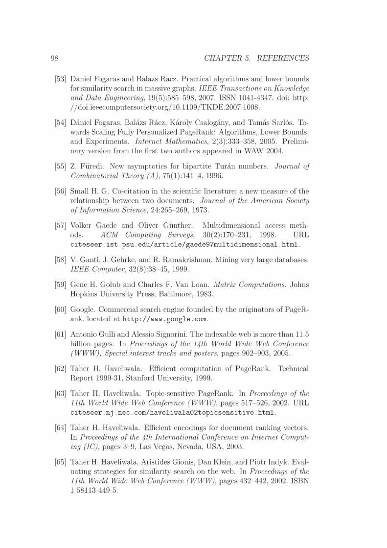
98 CHAPTER 5. REFERENCES
[53] Daniel Fogaras and Balazs Racz. Practical algorithms and lower boundsfor similarity search in massive graphs. IEEE Transactions on Knowledgeand Data Engineering, 19(5):585–598, 2007. ISSN 1041-4347. doi: http://doi.ieeecomputersociety.org/10.1109/TKDE.2007.1008.
[54] Daniel Fogaras, Balazs Racz, Karoly Csalogany, and Tamas Sarlos. To-wards Scaling Fully Personalized PageRank: Algorithms, Lower Bounds,and Experiments. Internet Mathematics, 2(3):333–358, 2005. Prelimi-nary version from the first two authors appeared in WAW 2004.
[55] Z. Furedi. New asymptotics for bipartite Turan numbers. Journal ofCombinatorial Theory (A), 75(1):141–4, 1996.
[56] Small H. G. Co-citation in the scientific literature; a new measure of therelationship between two documents. Journal of the American Societyof Information Science, 24:265–269, 1973.
[57] Volker Gaede and Oliver Gunther. Multidimensional access meth-ods. ACM Computing Surveys, 30(2):170–231, 1998. URLciteseer.ist.psu.edu/article/gaede97multidimensional.html.
[58] V. Ganti, J. Gehrke, and R. Ramakrishnan. Mining very large databases.IEEE Computer, 32(8):38–45, 1999.
[59] Gene H. Golub and Charles F. Van Loan. Matrix Computations. JohnsHopkins University Press, Baltimore, 1983.
[60] Google. Commercial search engine founded by the originators of PageR-ank. located at http://www.google.com.
[61] Antonio Gulli and Alessio Signorini. The indexable web is more than 11.5billion pages. In Proceedings of the 14th World Wide Web Conference(WWW), Special interest tracks and posters, pages 902–903, 2005.
[62] Taher H. Haveliwala. Efficient computation of PageRank. TechnicalReport 1999-31, Stanford University, 1999.
[63] Taher H. Haveliwala. Topic-sensitive PageRank. In Proceedings of the11th World Wide Web Conference (WWW), pages 517–526, 2002. URLciteseer.nj.nec.com/haveliwala02topicsensitive.html.
[64] Taher H. Haveliwala. Efficient encodings for document ranking vectors.In Proceedings of the 4th International Conference on Internet Comput-ing (IC), pages 3–9, Las Vegas, Nevada, USA, 2003.
[65] Taher H. Haveliwala, Aristides Gionis, Dan Klein, and Piotr Indyk. Eval-uating strategies for similarity search on the web. In Proceedings of the11th World Wide Web Conference (WWW), pages 432–442, 2002. ISBN1-58113-449-5.

99
[66] Taher H. Haveliwala, Sepandar Kamvar, and Glen Jeh. Ananalytical comparison of approaches to personalizing PageRank.Technical Report 2003-35, Stanford University, 2003. URLhttp://dbpubs.stanford.edu:8090/pub/2003-35.
[67] M. R. Henzinger, P. Raghavan, and S. Rajagopalan. Computing on datastreams. Technical Report 1998-011, DEC SRC, 1998.
[68] Monika R. Henzinger, Allan Heydon, Michael Mitzenmacher, and MarcNajork. Measuring index quality using random walks on the Web. InProceedings of the 8th World Wide Web Conference (WWW), pages 213–225, 1999.
[69] Monika R. Henzinger, Prabhakar Raghavan, and Sridhar Rajagopalan.Computing on data streams. In External Memory Algorithms, DIMACSBook Series vol. 50., pages 107–118. American Mathematical Society,1999. ISBN 0-8218-1184-3.
[70] Monika R. Henzinger, Allan Heydon, Michael Mitzenmacher, and MarcNajork. On near-uniform url sampling. In Proceedings of the 9th in-ternational World Wide Web conference on Computer networks, pages295–308, 2000. doi: http://dx.doi.org/10.1016/S1389-1286(00)00055-4.
[71] Jun Hirai, Sriram Raghavan, Hector Garcia-Molina, and AndreasPaepcke. WebBase: A repository of web pages. In Proceedings of the 9thWorld Wide Web Conference (WWW), pages 277–293, 2000.
[72] A. Hume, S. Daniels, and A. MacLellen. Gecko: Tracking a very largebilling system. In Proc. USENIX Ann. Technical Conference, pages 93–106, 2000.
[73] Piotr Indyk and Rajeev Motwani. Approximate near-est neighbors: Towards removing the curse of dimensional-ity. In Proceedings of the 30th ACM Symposium on The-ory of Computing (STOC), pages 604–613, 1998. URLciteseer.ist.psu.edu/article/indyk98approximate.html.
[74] Glen Jeh and Jennifer Widom. SimRank: A measure of structural-context similarity. In Proceedings of the 8th ACM International Confer-ence on Knowledge Discovery and Data Mining (SIGKDD), pages 538–543, 2002. URL http://dbpubs.stanford.edu:8090/pub/2001-41.
[75] Glen Jeh and Jennifer Widom. Scaling personalized web search. InProceedings of the 12th World Wide Web Conference (WWW), pages271–279. ACM Press, 2003. ISBN 1-58113-680-3. doi: http://doi.acm.org/10.1145/775152.775191.

100 CHAPTER 5. REFERENCES
[76] Thorsten Joachims. Optimizing search engines using clickthrough data.In KDD ’02: Proceedings of the eighth ACM SIGKDD internationalconference on Knowledge discovery and data mining, pages 133–142,New York, NY, USA, 2002. ACM. ISBN 1-58113-567-X. doi: http://doi.acm.org/10.1145/775047.775067.
[77] Sepandar Kamvar, Taher H. Haveliwala, Christopher Manning, andGene Golub. Exploiting the block structure of the web for computingPageRank. Technical Report 2003-17, Stanford University, 2003. URLciteseer.ist.psu.edu/kamvar03exploiting.html.
[78] Sepandar D. Kamvar, Taher H. Haveliwala, Christopher D. Manning,and Gene H. Golub. Extrapolation methods for accelerating PageRankcomputations. In Proceedings of the 12th World Wide Web Conference(WWW), pages 261–270. ACM Press, 2003. ISBN 1-58113-680-3. doi:http://doi.acm.org/10.1145/775152.775190.
[79] Maurice G. Kendall. Rank Correlation Methods. Hafner Publishing Co.,New York, 1955.
[80] M.M. Kessler. Bibliographic coupling between scientific papers. Ameri-can Documentation, 14:10–25, 1963.
[81] J. Kleinberg. Authoritative sources in a hyperlinked environment. Jour-nal of the ACM, 46(5):604–32, 1999.
[82] Jon Kleinberg. Authoritative sources in a hyperlinked envi-ronment. Journal of the ACM, 46(5):604–632, 1999. URLciteseer.nj.nec.com/article/kleinberg98authoritative.html.
[83] I. Kremer, N. Nisan, and D. Ron. On randomized one-round communi-cation complexity. Computational Complexity, 8(1):21–49, 1999. Errata,10(4):314–5, 2001.
[84] Eyal Kushilevitz and Noam Nisan. Communication Complexity. Cam-bridge University Press, 1997. ISBN 0-521-56067-5.
[85] Hsin-Tsang Lee, Derek Leonard, Xiaoming Wang, and Dmitri Loguinov.Irlbot: scaling to 6 billion pages and beyond. In WWW ’08: Proceedingof the 17th international conference on World Wide Web, pages 427–436, New York, NY, USA, 2008. ACM. ISBN 978-1-60558-085-2. doi:http://doi.acm.org/10.1145/1367497.1367556.
[86] Ronny Lempel and Shlomo Moran. Rank stability and rank similarityof link-based web ranking algorithms in authority connected graphs. InSecond Workshop on Algorithms and Models for the Web-Graph (WAW2003), 2003.

101
[87] Stefano Leonardi, editor. Algorithms and Models for the Web-Graph:Third International Workshop, WAW 2004, Rome, Italy, October 16,2004, Proceeedings, volume 3243 of Lecture Notes in Computer Science,2004. Springer. ISBN 3-540-23427-6.
[88] C.-S. Li and R. Ramaswami. Automatic fault detection, isolation, andrecovery in transparent all-optical networks. Journal of Lightwave Tech-nology, 15(10):1784–93, 1997.
[89] David Liben-Nowell and Jon Kleinberg. The link prediction problem forsocial networks. In Proceedings of the 12th Conference on Informationand Knowledge Management (CIKM), pages 556–559, 2003. ISBN 1-58113-723-0. doi: http://doi.acm.org/10.1145/956863.956972.
[90] Wangzhong Lu, Jeannette Janssen, Evangelos Milios, and Nathalie Jap-kowicz. Node similarity in networked information spaces. In Proceedingsof the Conference of the Centre for Advanced Studies on Collaborativeresearch, page 11, 2001.
[91] Ulrich Meyer, Peter Sanders, and Jop Sibeyn. Algorithms for MemoryHierarchies, Advanced Lectures. Springer-Verlag, Berlin, 2003.
[92] S. Muthukrishnan. Data streams: Algorithms and applications. Foun-dations and Trends in Theoretical Computer Science, 1(2), 2005.
[93] N. Nisan and E. Kushilevitz. Communication Complexity. CambridgeUniversity Press, Cambridge, UK, 1997.
[94] Open Directory Project (ODP). Open Directory Project (ODP).http://www.dmoz.org.
[95] Lawrence Page, Sergey Brin, Rajeev Motwani, and Terry Wino-grad. The PageRank citation ranking: Bringing order to theweb. Technical Report 1999-66, Stanford University, 1998. URLciteseer.nj.nec.com/page98pagerank.html.
[96] Christopher R. Palmer, Phillip B. Gibbons, and Christos Faloutsos.ANF: A fast and scalable tool for data mining in massive graphs. In Pro-ceedings of the 8th ACM International Conference on Knowledge Discov-ery and Data Mining (SIGKDD), pages 81–90. ACM Press, 2002. ISBN1-58113-567-X. doi: http://doi.acm.org/10.1145/775047.775059.
[97] Paat Rusmevichientong, David M. Pennock, Steve Lawrence, andC. Lee Giles. Methods for sampling pages uniformly fromthe world wide web. In AAAI Fall Symposium on UsingUncertainty Within Computation, pages 121–128, 2001. URLciteseer.ist.psu.edu/article/rusmevichientong01methods.html.

102 CHAPTER 5. REFERENCES
[98] G. Salton and C. Buckley. Term-weighting approaches in automatic textretrieval. Information Processing & Management, 24:513–523, 1988.
[99] G. Salton and M. McGill. Introduction to Modern Information Retrieval.McGraw-Hill, 1983.
[100] Tamas Sarlos, Andras A. Benczur, Karoly Csalogany, Daniel Fogaras,and Balazs Racz. To randomize or not to randomize: Space optimalsummaries for hyperlink analysis. In Proceedings of the 15th Interna-tional World Wide Web Conference (WWW), pages 297–306, 2006. Fullversion available at http://www.ilab.sztaki.hu/websearch/Publications/.
[101] Pavan Kumar C. Singitham, Mahathi S. Mahabhashyam, and PrabhakarRaghavan. Efficiency-quality tradeoffs for vector score aggregation. InProceedings of the 30th International Conference on Very Large DataBases (VLDB), pages 624–635, 2004.
[102] S. Stolfo, W. Fan, W. Lee, A. Prodromidis, and P. Chan. Cost-basedmodeling for fraud and intrusion detection: Results from the JAMproject. In Proc. DARPA Information and Survivability Conference andExposition, volume 2, pages 130–144, 2000.
[103] Torsten Suel and V. Shkapenyuk. Design and implementation of a high-performance distributed web crawler. In Proceedings of the 3rd IEEEInternational Conference on Data Engineering, February 2002.
[104] Danny Sullivan. Search engine size wars & google’s supplemental results.URL http://searchenginewatch.com/3071371.
[105] S. G. Tzafestas and P. J. Dalianis. Fault diagnosis in complex systemsusing artificial neural networks. In Proc. 3rd IEEE Conf. on ControlApplications, volume 2, pages 877–82, 1994.
[106] J. D. Ullman. The MIDAS data-mining project at Stanford. In Proc.1999 IEEE Symp. on Database Engineering and Applications, pages 460–4, 1999.
[107] J. S. Vitter. External memory algorithms and data structures: Dealingwith massive data. ACM Computing Surveys, 33(2):209–71, 2001.
[108] Ian H. Witten, Alistair Moffat, and Timothy C. Bell. Managing gigabytes(2nd ed.): Compressing and indexing documents and images. MorganKaufmann Publishers Inc., 1999. ISBN 1-55860-570-3.
[109] Gui-Rong Xue, Chenxi Lin, Qiang Yang, WenSi Xi, Hua-Jun Zeng, YongYu, and Zheng Chen. Scalable collaborative filtering using cluster-basedsmoothing. In SIGIR ’05: Proceedings of the 28th annual international

103
ACM SIGIR conference on research and development in information re-trieval, pages 114–121, New York, NY, USA, 2005. ACM Press. ISBN1-59593-034-5. doi: http://doi.acm.org/10.1145/1076034.1076056.
[110] K. Zarankiewicz. Problem P 101. Colloquium Mathematicum, 2:301,1951.

Index of Citations
Baeza-Yates and Ribeiro-Neto [1999],33, 46
Bar-Yossef and Gurevich [2007], 7Bar-Yossef et al. [2000], 15, 33Bar-Yossef et al. [2002], 60Bar-Yossef et al. [2004], 15, 33, 59, 65,
66Bar-Yossef [2002], 33Barroso et al. [2003], 9Boldi and Vigna [2004], 17, 26Bollobas [1978], 63Borodin et al. [2001], 11Brin and Page [1998], 11Broder et al. [2000], 42Broder [1997], 15, 33, 51Buchsbaum et al. [2004], 57, 60Chakrabarti et al. [1998], 33Chan et al. [1999], 57Chen et al. [2002], 17, 33Cohen [1997], 13, 15, 33Cortes et al. [2004], 57Costello et al. [], 7Dean and Ghemawat [2004], 17Dean and Henzinger [1999], 31Dwork et al. [2001], 25Eiron and McCurley [2003], 20Elkin and Zhang [2004], 60Fagin et al. [2003], 25Fagin et al. [2004], 25Fang et al. [1998], 57Feigenbaum et al. [2004], 60Feigenbaum et al. [2005], 60Fogaras and Racz [2004], 15, 32Fogaras and Racz [2005], 13, 15
Fogaras [2003], 16Furedi [1996], 61, 62Ganti et al. [1999], 57Gulli and Signorini [2005], 7Haveliwala et al. [2002], 33, 50Haveliwala et al. [2003], 11, 33Haveliwala [1999], 33Haveliwala [2002], 11, 12, 14, 16Haveliwala [2003], 25Henzinger et al. [1998], 57–60Henzinger et al. [1999], 15, 23, 33, 48Henzinger et al. [2000], 15, 33Hirai et al. [2000], 25, 32Hume et al. [2000], 57Indyk and Motwani [1998], 33Jeh and Widom [2002], 31, 33–35, 41Jeh and Widom [2003], 11–14, 16, 20,
25, 26Joachims [2002], 5Kamvar et al. [2003], 11, 12, 14, 20, 25Kendall [1955], 26Kleinberg [1999], 11, 31, 57Kremer et al. [1999], 59, 63Kushilevitz and Nisan [1997], 23, 48Lempel and Moran [2003], 22Li and Ramaswami [1997], 57Liben-Nowell and Kleinberg [2003], 31Lu et al. [2001], 31Muthukrishnan [2005], 58, 60Nisan and Kushilevitz [1997], 59Open Directory Project [ODP], 11, 50Page et al. [1998], 11, 12, 14, 16, 31–33Palmer et al. [2002], 15, 33Rusmevichientong et al. [2001], 15, 33
104

INDEX OF CITATIONS 105
Singitham et al. [2004], 25Stolfo et al. [2000], 57Suel and Shkapenyuk [2002], 25Sullivan [], 7Tzafestas and Dalianis [1994], 57Ullman [1999], 57Vitter [2001], 57Zarankiewicz [1951], 61de Kunder [], 7

106 INDEX OF CITATIONS

Acknowledgement
Above all I would like to thank my co-author and at the time fellow PhDstudent Daniel Fogaras for introducing me to the field of link-based searchalgorithms and the several years of fruitful collaboration that followed.
I would like to say special thanks to the leading research scientists of theData Mining and Web Search Group: Andras Benczur, who was my advisor,and Andras Lukacs. They have supported my career during my time at theHungarian Academy of Sciences, and supplied me with a constant stream ofvery diverse tasks ranging from CS research through software engineering oflarge-scale infrastructure systems to R&D grants work and public procurement,which have developed a versatile set of skills that turned out to be very helpfulin my further career. I am thankful to my colleagues and co-authors in theresearch group, Karoly Csalogany and Tamas Sarlos for implementing some ofour algorithms and doing experimental evaluation, and for all the feedback theygave during the research work that kept us on the right course. The qualityof our manuscripts and papers were singificantly improved by comments fromthe aforementioned people, as well as Lajos Ronyai, Daniel Marx, Glen Jeh,Andrew Twigg, Adam L. Buchsbaum and Raffaele Giancarlo. I would like toespecially thank to Ferenc Bodon, with whom I worked together for a longtime on a field of research outside this thesis.
I am especially grateful to Professors Lajos Ronyai, Andras Recski andBalint Toth, who, as the heads of the three departments related to my field(Algebra, Computer Science and Probability, respectively) have supported mydevelopment with advice, challenges and opportunities.
107