multi-modal scene understanding for robotic grasping
TRANSCRIPT

Multi-Modal Scene Understanding
for Robotic Grasping
JEANNETTE BOHG
Doctoral Thesis in Robotics and Computer Vision
Stockholm, Sweden 2011

TRITA-CSC-A 2011:17ISSN-1653-5723ISRN-KTH/CSC/A–11/17-SEISBN 978-91-7501-184-4
Kungliga Tekniska högskolanSchool of Computer Science and Communication
SE-100 44 StockholmSWEDEN
Akademisk avhandling som med tillstånd av Kungl Tekniska högskolan framläggestill offentlig granskning för avläggande av teknologie doktorsexamen i datalogifredagen den 16 december 2011 klockan 10.00 i Sal D2, Kungliga Tekniska högskolan,Lindstedtsvägen 5, Stockholm.
© Jeannette Bohg, November 17, 2011
Tryck: E-Print
iii
Abstract
Current robotics research is largely driven by the vision of creating anintelligent being that can perform dangerous, difficult or unpopular tasks.These can for example be exploring the surface of planet mars or the bottomof the ocean, maintaining a furnace or assembling a car. They can also bemore mundane such as cleaning an apartment or fetching groceries.
This vision has been pursued since the 1960s when the first robots werebuilt. Some of the tasks mentioned above, especially those in industrial man-ufacturing, are already frequently performed by robots. Others are still com-pletely out of reach. Especially, household robots are far away from being de-ployable as general purpose devices. Although advancements have been madein this research area, robots are not yet able to perform household chores ro-bustly in unstructured and open-ended environments given unexpected eventsand uncertainty in perception and execution.
In this thesis, we are analyzing which perceptual and motor capabilitiesare necessary for the robot to perform common tasks in a household scenario.In that context, an essential capability is to understand the scene that therobot has to interact with. This involves separating objects from the back-ground but also from each other. Once this is achieved, many other tasksbecome much easier. Configuration of objects can be determined; they canbe identified or categorized; their pose can be estimated; free and occupiedspace in the environment can be outlined. This kind of scene model can theninform grasp planning algorithms to finally pick up objects. However, sceneunderstanding is not a trivial problem and even state-of-the-art methods mayfail. Given an incomplete, noisy and potentially erroneously segmented scenemodel, the questions remain how suitable grasps can be planned and howthey can be executed robustly.
In this thesis, we propose to equip the robot with a set of predictionmechanisms that allow it to hypothesize about parts of the scene it has notyet observed. Additionally, the robot can also quantify how uncertain itis about this prediction allowing it to plan actions for exploring the sceneat specifically uncertain places. We consider multiple modalities includingmonocular and stereo vision, haptic sensing and information obtained througha human-robot dialog system. We also study several scene representations ofdifferent complexity and their applicability to a grasping scenario.
Given an improved scene model from this multi-modal exploration, graspscan be inferred for each object hypothesis. Dependent on whether the objectsare known, familiar or unknown, different methodologies for grasp inferenceapply. In this thesis, we propose novel methods for each of these cases. Fur-thermore, we demonstrate the execution of these grasp both in a closed andopen-loop manner showing the effectiveness of the proposed methods in real-world scenarios.
iv
Thank you, x y!for
Alper
Matt
Nicky
Zuspruch und Unterstützung
Hendrik
Beatriz
Marin
Omid
Christiane
Oscar
Dan
Stefan
Darius
FlorianP
Tamim
Hossein
Gabriel
Gesa
Henry
Xavier
Sebastian
Claudia
Ville
Thomas
Matei
Den Hinweis, wann ich mir mal wieder die Haare kämmen müsste
Moritz
Games and Cake
Inspiration
Kate
Iasonus
Babak
Gustavo
Stammtisch und RadebergerBeer
Cheng
Franziska
John
Jana
Vahid
Oma
Marten
Karthik
Renaud
Collaboration Mentoring
Chavo
Jeanna
Frine
Andrzej
Antonio
Antonis
Dani
EU
David
Heiner
Josephine
Kaijen
Alessandro
threadpool
zu Hause
Photography
Die guten Dresdner Zeiten
Higinio
Magnus
Xavi
GraspProject
Conny
Axel
Heydar
Beard
Kathi
Papa
Nikos
Tobias
Melanie
Being an amazing roomie
Geert
141-crowd
Opa
Javier
Erdbeermarmelade, eingelegte Gurken und Sonntagsbraten
Unsere alte Freundschaft
Carl-Henrik
Carsten
Marianna
Ioannis
KaiW
Ylva
Svenska
For teaching their sons how to cook
Mama
Jarmo
Jan-Olof
CVAP
Florian
Lazaros
StefanS
StefanU
Susanne
Walter
Christian
Tener un corazon tan grande como el sombrero de un picador
Kai
Proof-reading
Urlaubspläne
chrisarndt
Birgit
Niklas
Yasemin
XavisMom
Miro
Martin
Aitor
Kristoffer
Coci
Janne
MartinS
JaviersMom
For not being roboticists
Supervision and Support
MarkusP
MarkusV
Contents
1 Introduction 3
1.1 An Example Scenario . . . . . . . . . . . . . . . . . . . . . . . . . . . 41.2 Towards Intelligent Machines - A Historical Perspective . . . . . . . . . 61.3 This Thesis . . . . . . . . . . . . . . . . . . . . . . . . . . . . . . . . 101.4 Outline and Contributions . . . . . . . . . . . . . . . . . . . . . . . . . 121.5 Publications . . . . . . . . . . . . . . . . . . . . . . . . . . . . . . . . 14
2 Foundations 17
2.1 Hardware . . . . . . . . . . . . . . . . . . . . . . . . . . . . . . . . . . 172.2 Vision Components . . . . . . . . . . . . . . . . . . . . . . . . . . . . 192.3 Discussion . . . . . . . . . . . . . . . . . . . . . . . . . . . . . . . . . 24
3 Active Scene Understanding 25
4 Predicting and Exploring Scenes 29
4.1 Occupancy Grid Maps for Grasping and Manipulation . . . . . . . . . . 304.2 Height Map for Grasping and Manipulation . . . . . . . . . . . . . . . 464.3 Discussion . . . . . . . . . . . . . . . . . . . . . . . . . . . . . . . . . 64
5 Enhanced Scene Understanding through Human-Robot Dialog 67
5.1 System Overview . . . . . . . . . . . . . . . . . . . . . . . . . . . . . 685.2 Dialog System . . . . . . . . . . . . . . . . . . . . . . . . . . . . . . . 685.3 Refining the Scene Model through Human-Robot Interaction . . . . . . 695.4 Experiments . . . . . . . . . . . . . . . . . . . . . . . . . . . . . . . . 755.5 Discussion . . . . . . . . . . . . . . . . . . . . . . . . . . . . . . . . . 80
6 Predicting Unknown Object Shape 81
6.1 Symmetry for Object Shape Prediction . . . . . . . . . . . . . . . . . . 826.2 Experiments . . . . . . . . . . . . . . . . . . . . . . . . . . . . . . . . 906.3 Discussion . . . . . . . . . . . . . . . . . . . . . . . . . . . . . . . . . 98
7 Generation of Grasp Hypotheses 101
v

vi CONTENTS
7.1 Related Work . . . . . . . . . . . . . . . . . . . . . . . . . . . . . . . 1037.2 Grasping Known Objects . . . . . . . . . . . . . . . . . . . . . . . . . 1167.3 Grasping Unknown Objects . . . . . . . . . . . . . . . . . . . . . . . . 1267.4 Grasping Familiar Objects . . . . . . . . . . . . . . . . . . . . . . . . . 1297.5 Discussion . . . . . . . . . . . . . . . . . . . . . . . . . . . . . . . . . 150
8 Grasp Execution 153
8.1 Open Loop Grasp Execution . . . . . . . . . . . . . . . . . . . . . . . 1538.2 Closed-Loop Grasp Execution . . . . . . . . . . . . . . . . . . . . . . . 1578.3 Discussion . . . . . . . . . . . . . . . . . . . . . . . . . . . . . . . . . 167
9 Conclusions 169
A Covariance Functions 173
Bibliography 177
Notation
Throughout this thesis, the following notational conventions are used.
• Scalars are denoted by italic symbols, e.g., a, b, c.
• Vectors, regardless of dimension, are denoted in bold lower-case symbols,x = (x, y)T .
• Sets are indicated by calligraphic symbols, e.g., P, Q, R. The cardinalityof these sets is denoted by capital letters such as N, M, K. As a compactnotation for a set X containing N vectors xi, we will use {xi}N .
• In this thesis, we frequently deal with estimates of vectors. They are indicatedby a hat superscript, e.g., x. They also can be referred to as a posterioriestimates in contrast to a priori estimates. The latter are denoted by anadditional superscript. This can either be a minus, e.g., x− for estimates intime, or a plus, e.g., x+ for estimates in space.
• Functions are denoted by italic symbols followed by their arguments in paren-theses, e.g., f(·), g(·), k(·, ·). An exception is the normal distribution wherewe adopt the standard notation of N (µ, Σ).
• Matrices, regardless of dimension, are denoted as bold-face capital letters,e.g., A, B, C.
• Frames of reference or coordinate frames are denoted by sans-serif capitalletters, e.g., W, C. In this thesis, we convert coordinates mostly between thefollowing three reference frames: the world reference frame W, the cameracoordinate frame C and the image coordinate frame I. Vectors that are relatedto a specific reference frame are annotated with the according superscript, e.g.,xW.
• Sometimes in this thesis, we have to distinguish between the left and rightimage of a stereo camera. We label vectors referring to the left camera systemwith a subscript l and analogous with r for the right camera system, e.g.,xl, xr.
1
2 CONTENTS
• A finger on our robotic hand is padded with a tactile sensor matrices. Oneis on the distal and one on the proximal phalanx. Measurements from thesesensors are either labeled with subscript d or p.
• The subscript t refers to a specific point in time.
• In this thesis, we develop prediction mechanism that enable the robot to makepredictions about unobserved space in its environment. We label the set oflocations that has already been observed with subscript k for known. Thepart that is yet unknown is labeled with subscript u.
1
Introduction
The idea of creating an artificial being is quite old. Even before the word robotgot coined by Karel Čapek in 1920, the concept appeared frequently in litera-ture and other artwork. The idea can already be observed in preserved records ofancient automated mechanical artifacts [206]. In the beginning of the 20th cen-tury, advancements in technology led to the birth of the science fiction genre.Among other topics, the robot became a central figure of stories told in books andmovies [217, 82]. The first physical robots had to await the development of thenecessary underlying technology in the 1960s. Interestingly, already in 1964 NamJune Paik in collaboration with Shuya Abe built the first robot to appear in thefield of new media arts: Robot K456 [61, pg. 73].
The fascination of humans with robots stems from a dichotomy in how we per-ceive them. One the one hand, we strive for replicating our consciousness, intelli-gence and physical being but with characteristics that we associate with technology:regularity, efficiency, stability and power. Such an artificial being could then existbeyond human limitations, constraints and even responsibility [217]. In a way, thisstriving reflects the ancient search for immortal life. On the other hand, there isthe fear that once such a robot exists we may loose control over our own creation.In fact, we would have created our own replacement [82].
Exactly this conflict is subject of most of the robot stories reaching from theclassic ones like R.U.R. (Rossum’s Universal Robots) by Karel Čapek and FritzLang’s Metropolis to the newer ones such as James Cameron’s Terminator andAlex Proyas’ I, Robot. Geduld [86] divided the corpus of stories into material about"god-sanctioned” and "sacrilegious creation" to reflect the simultaneous attractionand recoil. He places the history of real automata completely aside from this.
In current robotics research, the striving for replicating human intelligence iscompletely embraced. Robots are celebrated as accomplishments that demonstratehuman artifice. When reading the introductions of many recent books, PhD thesesand articles on robotics research, the arrival of service robots in our everyday life ispredicted to happen in the near future [192, 174, 121], already "tomorrow” [206] oris claimed to have already happened [177]. Rusu [192] and Prats [174] emphasize thenecessity of service robotics with regard to the aging population of Europe, Japanand the USA. Machines equipped with ideal physical and cognitive capabilities
3
4 CHAPTER 1. INTRODUCTION
are thought to care for people who became physically and cognitively limited ordisabled. Although robotics celebrated its 50th birthday this year, only recentlythe topic of roboethics has been coined and a roadmap published by Veruggio [226].In that sense, the art community is somewhat ahead of the robotics community indiscussing implications of technological advancement.
The question why robotics research shows only little interest in these topicsremains. We argue that this is because robots are not perceived by roboticiststo have even remotely achieved the level of intelligence that we believe to be nec-essary to replace us. In reality, we are far away from having a general purposerobot as envisioned in many science fiction stories. Instead we are at the stage ofthe specific purpose robot. Especially in industrial manufacturing, robots are om-nipresent in assembling specific products. Other robots have shown to be capable ofautonomous driving in environments of different complexities and constraints. Re-garding household scenarios, robots already vacuum-clean apartments [105]. Othertasks like folding towels [141], preparing pancakes [24] or clear a table as in thethesis at hand have been demonstrated on research platforms. However, to letrobots perform these task robustly in unstructured and open-ended environmentsgiven unexpected events and uncertainty in perception and execution is an ongoingresearch effort.
1.1 An Example Scenario
Robots are good at many things that are hard for us. This involves the aspectsmentioned before like regularity, efficiency, stability and power but also games likechess and jeopardy in which, although not robots in the strict sense, supercomputershave recently beaten human masters. However, robots appear to be not very goodin many things that we perform effortlessly. Examples are grasping and dexterousmanipulation of everyday objects or learning about new objects for recognizingthem later on. In the following, we want to exemplify this with the help of a simplescenario.
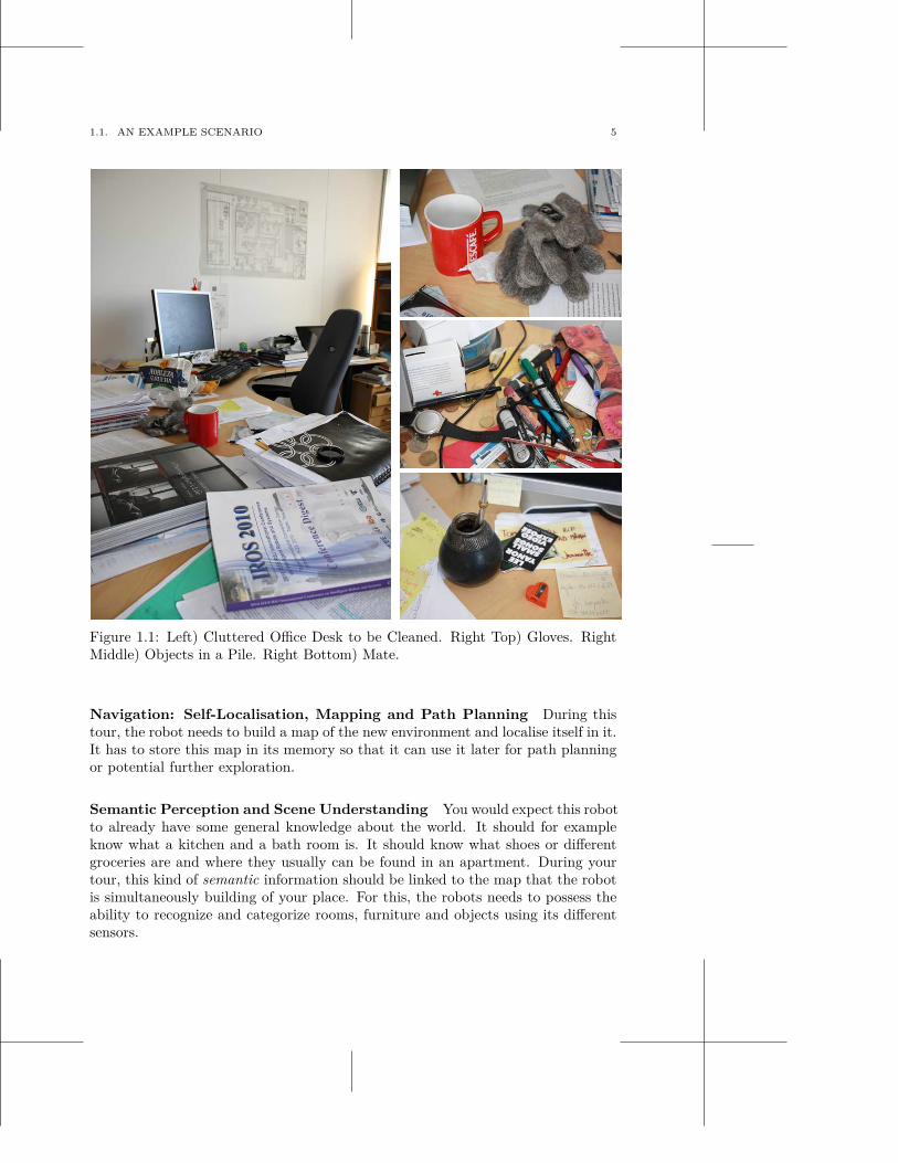
Figure 1.1 shows an office desk. Imagine that you ordered a brand-new roboticbutler and you want it to clean that desk for you. What kind of capabilities doesit need for fulfilling this task? In the following, we list a few of them.
Recognition of Human Action and Speech Just like with a real butler whois new to your place, you need to give the robot a tour. This involves showingit all the rooms and explaining what function they have. Besides that, you mayalso want to point out places like cupboards in the kitchen or shoe cabinets inthe corridor so that it knows where to store certain objects. For the robot toextract information from this tour, it needs to be able to understand human speechbut also human actions like walking behavior or pointing gestures. Only then, itcan generate the appropriate behavior by itself like for example following, askingquestions or pointing at things.
1.1. AN EXAMPLE SCENARIO 5
Figure 1.1: Left) Cluttered Office Desk to be Cleaned. Right Top) Gloves. RightMiddle) Objects in a Pile. Right Bottom) Mate.
Navigation: Self-Localisation, Mapping and Path Planning During thistour, the robot needs to build a map of the new environment and localise itself in it.It has to store this map in its memory so that it can use it later for path planningor potential further exploration.
Semantic Perception and Scene Understanding You would expect this robotto already have some general knowledge about the world. It should for exampleknow what a kitchen and a bath room is. It should know what shoes or differentgroceries are and where they usually can be found in an apartment. During yourtour, this kind of semantic information should be linked to the map that the robotis simultaneously building of your place. For this, the robots needs to possess theability to recognize and categorize rooms, furniture and objects using its differentsensors.
6 CHAPTER 1. INTRODUCTION
Learning When the robot leaves its factory, it is probably equipped with a lot ofknowledge about the world it is going to encounter. However, the probability thatit is confronted with rooms of an ambiguous function and objects it has never seenbefore is quite high. The robot needs to detect these gaps in its world knowledgeand attempt to close them. This may involve asking you to elaborate on somethingor to build a representation of an unknown object grounded in the sensory data.
Higher-Level Reasoning and Planning After the tour, the robot then maybe expected to finally clean this desk shown in Figure 1.1. If we assume that itrecognized the objects on the table, it now needs to plan what to do with them. Itcan for example leave them there, bring them to a designated place or throw theminto the trash. To make these decisions, it has to consult its world knowledge inconjunction with the semantic map it has just built of you apartment. The cupfor example may pose a conflict between its world knowledge (in which cups areusually in the kitchen) and the current map it has of the world. To resolve thisconflict, it needs to form a plan to align these two. A plan may involve any kind ofinteraction with the world be it asking your for assistance, grasping something orkeep exploring the environment.
Grasping and Manipulation Once the robot decided to pick up something tobring it somewhere else, it needs to execute this plan. Grasping and manipulationof objects demands the formation of low level motion plans that are robust on theone hand and flexible on the other. They need to be executed while facing noise,uncertainty and potentially unforeseen dynamic changes in the environment.
All of these capabilities in itself are the subject of ongoing research efforts inmostly separate communities. As the title of this thesis suggest, we are mainly con-cerned with scene understanding for robotic grasping and manipulation. Especiallyfor scenes as depicted in Figure 1.1, this poses a challenging problem to the robot.Although a child would be able to accomplish to grasp the shown objects withoutany problem, it has yet not been shown that a robot could perform equally wellwithout introducing strong assumptions.
1.2 Towards Intelligent Machines - A Historical Perspective
Since the beginning of robotics, pick and place problems from a table top have beenstudied [77]. Although the goal remained the same over the years, the differentapproaches were rooted in the paradigms on Artificial Intelligence (AI) of theirtime. One of the most challenging problems that has been approached over andover again, is to define what intelligence actually means. Recently, Pfeifer andBongard [171] even refuse to define this concept given what they claim to be themere absence of a good definition. In this section, we will briefly summarize someof the major views on intelligence.
1.2. TOWARDS INTELLIGENT MACHINES - A HISTORICAL PERSPECTIVE 7
World
CentralProcessor
Action Perception
Figure 1.2: Traditional Model of an Intelligent System.
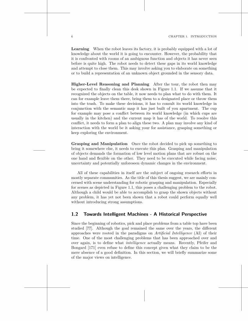
The traditional view is dominated by the physical symbol system hypothesis. Itstates that any system exhibiting intelligence can be proven to be a physical sym-bol system and any physical symbol system of sufficient size will exhibit intelligentbehavior [160, 207]. Figure 1.2 shows a schematic of the traditional model of in-telligence exhibited by humans or machines. The central component is a symbolicinformation processor that is able to manipulate a set of symbols potentially part ofwhole expressions. It can create, modify, reproduce or delete symbols. Essentially,such a symbol system can be modelled as a Turing machine. Therefore it followsthat intelligent behavior can be exhibited by todays computers. The symbols arethought to be amodal, i.e., completely independent of the kind of sensors and ac-tuators available to the system. The input to the central processor is providedby perceptual modules that convert sensory input into amodal symbols. The out-put is generated though action modules that use amodal symbolic descriptions ofcommands.
Turing [221] proposed an imitation game to re-frame the question “Can machinesthink?” that is now known as the famous Turing Test. The proposed machines arecapable of reading, writing and manipulating text without the need to understandits meaning. The problem of converting between real world percepts and amodalsymbols is thereby circumvented as well as conversion between symbolic commandsand real world motor commands. The hope was that this will be solved at somelater point. In the early days of AI research, a lot of progress was made in forexample theorem proofers, blocks world scenarios or artificial systems that couldtrick humans to believe that they were humans as well. However, early approachescould not be shown to translate to more complex scenarios [191]. In [171], Brooksnoted that “Turing modeled what a person does, not what a person thinks”. Alsothe behavioral studies on which Simon’s thesis [207] of physical symbol systems rest,can be seen in that light: humans solving cryptarithmetic problems, memorizing orperforming tasks that use natural language.
The view of physical symbol system has been challenged on several grounds. Inthe 1980s connectionist models became largely popular [191]. The most prominent
8 CHAPTER 1. INTRODUCTION
World
PerceptionAction
Figure 1.3: Model of an Intelligent System from the Viewpoint of BehavioralRobotics.
representative is the artificial neural network that is seen as a simple model ofthe human brain. Instead of a central processor, a neural network consists of anumber of simple interconnected units. Intelligence is seen as emergent within thisnetwork. Connectionist models have been shown to be far less domain specific andmore robust to noise. However according to Simon [207], it has yet to be shownthat complex thinking and problem solving can be modelled with connectionistapproaches. Nowadays, symbol systems and connectionist approaches are seen ascomplementary [191].
A different case has been argued by the supporters of the Physical SymbolGrounding Hypothesis. Instead of criticizing the structure of the proposed intel-ligent system, it re-considers the assumed amodality of the symbols. Its claim isthat to build a system that is truly intelligent, it has to have its symbols groundedin the physical world. In other words, it has to understand the meaning of thesymbols [96]. However, no perception system has yet been build that robustlyoutputs a general purpose symbolic representation of the perceived environment.Furthermore, perception has been claimed to be active and task dependent. Givendifferent tasks, different parts of the scene or different aspects of it may be rel-evant [22]. The the same percept can be interpreted differently. Therefore, noobjective truth exists [159].
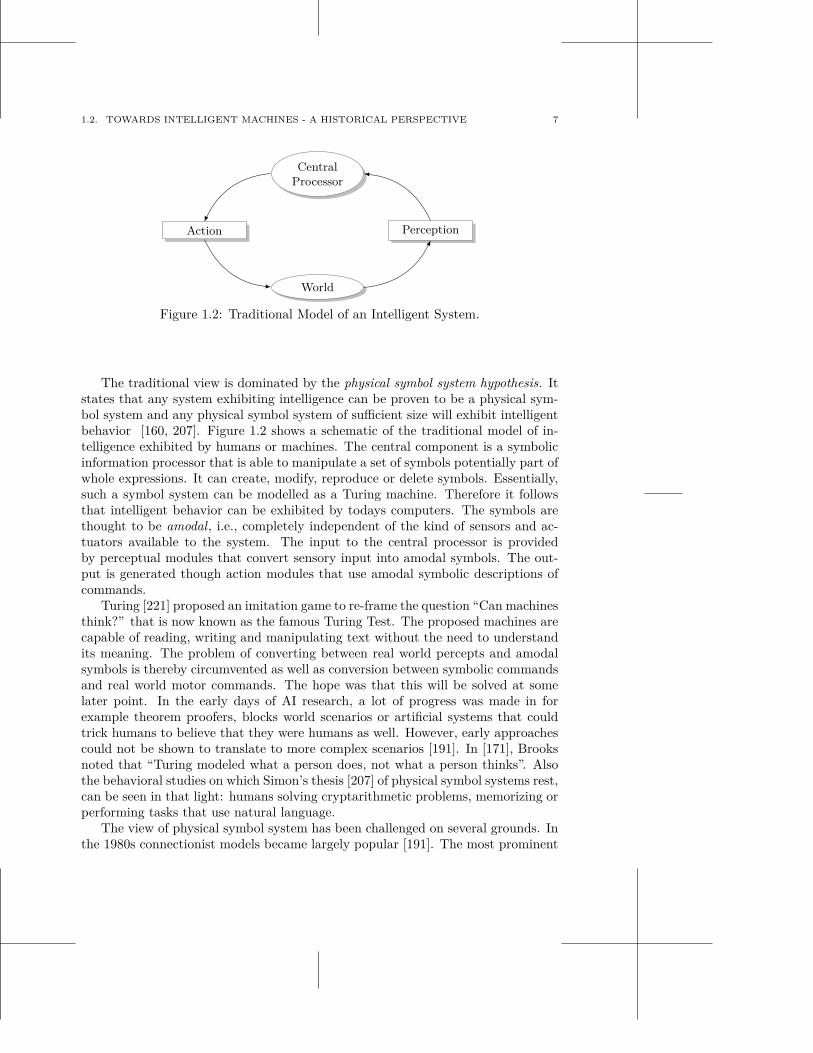
Brooks [46, 47] has carried this view to its extreme and asks whether intelligenceneeds any representations at all. Figure 1.3 shows the model of an intelligentmachine that completely abondons the need for representations. Brooks coined thesentence: The world is its own best model. The more details of the world you store,the more you need to keep up-to-date. He proposes to dismiss any intermediaterepresentation that interfaces between the world and computational modules as wellas in between computational modules. Instead, the system should be decomposedinto subsystem by activities that describe patterns of interactions with the world.As outlined in Figure 1.3, each subsystems tightly connects sensing to actions, andsenses whatever necessary and often enough to accomodate for dynamic changesin the world. No information is transferred between submodules. Instead, they
1.2. TOWARDS INTELLIGENT MACHINES - A HISTORICAL PERSPECTIVE 9
World
Prediction
Action Perception
Figure 1.4: Model of an Intelligent System from the Viewpoint of Grounded Cog-nition
compete for control of the robot through a central system. People have challengedthis view as being only suitable for creating insect-like robots without a proof thathigher cognitive functions are possible to achieve [51]. This approach is somehowsimilar to the Turing test in that it is claimed that if the behavior of the machineis intelligent in the eye of the beholder, then it is intelligent. Parallels can also bedrawn to Simon [207] in which an intelligent system is seen as essentially a verysimple mechanism. Its complexity is a mere reflection of the complexity of theenvironment.
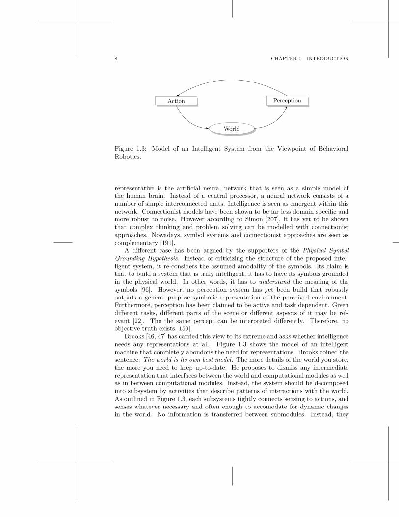
Figure 1.4 shows the schematic of an intelligent agent as envisioned for examplein psychology and neurophysiology. The field of Grounded Cognition focuses onthe role of simulation as exhibited by humans in behavioral studies [23]. Thenotion of amodal symbols that reside in semantic memory separate from the brain’smodal system for perception, action and introspection is rejected. Symbols areseen as to be grounded and stored in a multi-modal way. Simulation is a re-enactment of perceptual, motor and introspective states acquired during a specificexperience with the world, body and mind. It is triggered when knowledge isneeded to represent a specific object, category, action or situation. In that sense itis compatible with other theories as for example the simulation theory [84] or thecommon-coding theory of action and perception [176]. Through the discovery of theso-called Mirror neurons (MNs), these models gained momentum [185]. MNs havefirst been discovered in the F5 area of a monkey brain. During the first experiments,this area has been monitored during grasping actions. It was discovered that thereare neurons that fire both, when a grasping action is performed by the recordedmonkey and when this monkey observes the same action performed by anotherindividual. Interestingly, this action has to be goal directed which is in accordancewith the common-coding theory. Its main claim is that perception and action sharea common representational domain. Evidence from behavioral studies on humansshowed that actions are planned and controlled in terms of their effect [176]. Thereis also strong evidence that MNs exist in the human brain. Etzel et al. [74] testedthe simulation theory through standard machine learning techniques. The authors
10 CHAPTER 1. INTRODUCTION
trained a classifier on functional magnetic resonance imaging (fMRI) recorded fromhumans while hearing either of two actions. They showed that the same classifiercan also distinguish between these actions when provided fMRI data that is recordedfrom the same person performing them.
Up till now, no agreement has been reached on whether a central representa-tional system is used or a distributed one. Also no computational model has yetbeen proposed in the field of psychology or neurophysiology [23]. However, thereare some examples in the field of robotics following the general concept of groundedcognition. Ballard [22] introduces the concept of Animate Vision that aims at un-derstanding visual processing in the context of the tasks and behaviors the visionsystem is currently engaged in. In this paradigm, the need for maintaining a detailmodel of the world is avoided. Instead, real-time computation of a set of sim-ple visual features is emphasized such that task relevant representations can berapidly computed on demand. Christensen et al. [51] present a system for keepingmulti-modal representations of an entity in memory and refining them in parallel.Instead of one monolithic memory system, representations are shared among sub-systems. A binder is proposed for connecting each representation to one entity inmemory. This can be related to the Prediction box in Figure 1.4. Through thisbinding, perception of one modality corresponding to an entity could predict theother modalities associated with the same entity in memory. Another example ispresented by Kjellström et al. [116]. The authors show that the simultaneous ob-servation of two separate modalities (action and object features) helps to categorizeboth of them.
1.3 This Thesis
We are specifically concerned with perception for grasping and manipulation. Thepreviously mentioned theories stemming from psychology and neurophysiology arestudying the tight link between perception and action. They place the concept ofprediction through simulation into their focus. In this thesis, we will equip a robotwith mechanisms to predict unobserved parts of the environment and the effects ofits actions. We will show how this helps to efficiently explore the environment butalso how it improves perception and manipulation.
We will study this approach in a table top scenario populated with either known,unknown or familiar objects. As already outlined in the example scenario in Sec-tion 1.1, scene understanding is one important capability of a robot. In specific thisinvolves segmentation of objects from each other and from the background. Oncethis is achieved, many other tasks become much easier. Configuration of objects onthe table can be determined; they can be identified or categorized; their pose canbe determined; free and occupied space in the environment can be outlined. Thiskind of scene model can then inform grasp inference mechanisms to finally graspsobjects from the table top.
In Figure 1.1, we can observe why scene understanding is challenging. On the
1.3. THIS THESIS 11
Prediction
Action Perception
Prediction
Action Perception
Real World
Simulated World
Figure 1.5: Schematic of this thesis. Given some observations of the real world,the state of the world can be estimated. This can be used to predict unobservedparts of the scene (Prediction box) as formalized in Equation 1.1. It can be used topredict action outcomes (Action box) as formalized in Equation 1.2 and to predictwhat certain sensors should perceive (Perception box) as in Equation 1.3 and 1.4.
depicted office desk, there are piles of clutter for which even humans have problemsto separate them visually into single objects. Deformable objects like gloves areshown that come in very many different shapes and styles. Still we are able torecognize them correctly even though we might not have seen this specific pair everbefore. And there are objects that are completely unknown to us. Independent ofthis, we would be able to grasp them.
Figure 1.5 is related to Figure 1.4 by adopting the notion of prediction into theperception-action loop. On the left side, you see the real world. It can be perceivedthrough the sensors the robot is equipped with. This is an active process in whichthe robot can choose what to perceive by moving through the environment or bychanging it using its different actuators. On the left, you see a visualisation of thecurrent model the robot has of its environment.
This model makes simulation explicit in that perception feeds into memory toupdate a multi-modal representation of the current scene of interest. This scene isestimated at discrete points in time t to be in a specific state xt. This estimate isthen used to implement prediction in three different ways.
12 CHAPTER 1. INTRODUCTION
• Based on earlier observations, we have a partial estimate of the state of thescene xt. Given this estimate and some prior knowledge, we can predictunobserved parts of it to obtain an a priori state estimate:
x+t = g(xt) (1.1)
• Given the current state estimate, some action u and a process model, we canpredict how the scene model will change over time to obtain a different apriori state estimate:
x−t+1 = f(u, xt) (1.2)
• Given an a priori state estimate of the scene, we can predict what differentsensor modalities should perceive
zt = h(x+t ) (1.3)
orzt+1 = h(x−
t+1) (1.4)
These functions can be associated with the boxes positioned around the simulatedenvironment on the right hand side of Figure 1.5. While the Prediction box refersto prediction in space and is related to Equation 1.1, the Action box stands forprediction in time and the implementation of Equation 1.2. The Perception boxrepresents the prediction of sensor measurements as in Equation 1.3 and 1.4. Thescene model serves as a container representation that integrates multi-modal sensoryinformation as well as predictions. In this thesis, we study different kinds of scenerepresentations and their applicability for grasping and manipulation.
Independent of the specific representation, we are not only interested in a pointestimate of the state. Instead, we consider the world state as a random variablethat follows a distribution xt ∼ N (xt, Σt) with the state estimate as the meanand a variance Σt. This variance is estimated based on the assumed divergencebetween the output of the functions g(·), f(·) and h(·) and the unknown real value.It quantifies the uncertainty of the current state estimate.
In this thesis, we are proposing approaches that implement the function g(·)in Equation 1.1 to make predictions about space. We will demonstrate that theresulting a priori state estimate x+
t and the associated variance Σ+t can be used for
either (i) guiding exploratory actions to confirm particularly uncertain areas in thecurrent scene model, (ii) comparing predicted observations zt or actions outcomeswith the real observations zt and update the state estimate and variance accordinglyto obtain an a posteriori estimate or (iii) for exploiting the prediction in using itfor executing an action to achieve a given goal.
1.4 Outline and Contributions
This thesis is structured as follows:
1.4. OUTLINE AND CONTRIBUTIONS 13
Chapter 2 – Foundations
Chapter 2 introduces the hardware and software foundation of this thesis. Theapplied vision systems have been developed and published prior to this thesis andare only briefly introduced here.
Chapter 3 – Active Scene Understanding
The chapter introduces the problem of scene understanding and motivates the ap-proach followed in this thesis.
Chapter 4 – Predicting and Exploring a Scene
Chapter 4 is the first of the three chapters that propose different prediction mecha-nisms. Here, we study a classical occupancy grid and a height map as a representa-tion for a table top scene. We propose a method for multi-modal scene explorationwhere initial object hypotheses formed by active visual segmentation are confirmedand augmented through haptic exploration with a robotic arm. We update thecurrent belief about the state of the map with the detection results and predict yetunknown parts of the map with a Gaussian Process. We show that through theintegration of different sensor modalities, we achieve a more complete scene model.We also show that the prediction of the scene structure leads to a valid scene repre-sentation even if the map is not fully traversed. Furthermore, we propose differentexploration strategies and evaluate them both in simulation and on our roboticplatform.
Chapter 5 – Enhanced Scene Understanding through Human-Robot
Dialog
While Chapter 4 is more focussed on the prediction of occupied and empty spacein the scene, this chapter proposes a method for improving the segmentation ofobjects from each other. Our approach builds on top of state-of-the-art computervision segmenting stereo reconstructed point clouds into object hypotheses. In col-laboration with Matthew Johnson-Roberson and Gabriel Skantze this process iscombined with a natural dialog system. By putting a ‘human in the loop’ and ex-ploiting the natural conversation of an advanced dialogue system, the robot gainsknowledge about ambiguous situations beyond its own resolution. Specifically, weare introducing an entropy-based system allowing the robot to predict which ob-ject hypotheses might be wrong and query the user for arbitration. Based on theinformation obtained from the human-to-robot dialog, the scene segmentation canbe re-seeded and thereby improved. We analyse quantitatively what features arereliable indicators of segmentation quality. We present experimental results on realdata that show an improved segmentation performance compared to segmentationwithout interaction and compared to interaction with a mouse pointer.
14 CHAPTER 1. INTRODUCTION
Chapter 6 – Predicting Unknown Object Shape
The purpose of scene understanding is to plan successful grasps on the object hy-potheses. Even if these hypotheses are correctly corresponding only to one object,we commonly do not know the geometry of their backside. The approach to objectshape prediction proposed in this chapter aims at closing the knowledge gaps inthe robot’s understanding of the world. It is based on the observation that manyobjects in a service robotic scenario possess symmetries. We search for the optimalparameters of these symmetries given visibility constraints. Once found, the pointcloud is completed and a surface mesh reconstructed. This can then be providedto a simulator in which stable grasps and collision-free movements are planned.We present quantitative experiments showing that the object shape predictions arevalid approximations of the real object shape.
Chapter 7 – Generation of Grasp Hypotheses
In this chapter, we will show how the object hypotheses that have been formedthrough different methods can be used to infer grasps. In the first section, wereview existing approaches divided into three categories: grasping known, unknownor familiar objects. Given these different kinds of prior knowledge, the problem ofgrasp inference reduces to either object recognition and pose estimation, findingsimilarity metric between functionally similar objects or developing heuristics formapping grasps to object representations. For each case, we propose our ownmethods that extend the existing state of the art.
Chapter 8 – Grasp Execution
Once grasp hypotheses have been inferred, they need to be executed. We demon-strate the approaches proposed in Chapter 7 in an open-loop fashion. In collab-oration with Beatriz Léon and Javier Felip, experiments on different platform areperformed. This is followed by a review of the existing closed-loop approachestowards grasp execution. Although there are a few exceptions, they are usuallyfocussed on either the reaching trajectory or the grasp itself. We will demonstratein collaboration with Xavi Gratal and Javier Romero visual and virtual visual ser-voing to execute grasping of known or unknown objects. This helps in controllingthe reaching trajectory such that the end effector is accurately aligned with theobject prior to grasping.
1.5 Publications
Parts of this thesis have previously been published as listed in the following.
1.5. PUBLICATIONS 15
Conferences
[1] Niklas Bergström, Jeannette Bohg, and Danica Kragic. Integration of visualcues for robotic grasping. In Computer Vision Systems, volume 5815 of LectureNotes in Computer Science, pages 245–254. Springer Berlin / Heidelberg, 2009.
[2] Jeannette Bohg and Danica Kragic. Grasping familiar objects using shape con-text. In International Conference on Advanced Robotics (ICAR), pages 1 –6,Munich, Germany, June 2009.
[3] Jeannette Bohg, Matthew Johnson-Roberson, Mårten Björkman, and DanicaKragic. Strategies for Multi-Modal Scene Exploration. In IEEE/RSJ Interna-tional Conference on Intelligent Robots and Systems (IROS), pages 4509 –4515,October 2010.
[4] Jeannette Bohg, Matthew Johnson-Roberson, Beatriz León, Javier Felip, XaviGratal, Niklas Bergström, Danica Kragic, and Antonio Morales. Mind theGap - Robotic Grasping under Incomplete Observation. In IEEE InternationalConference on Robotics and Automation (ICRA), May 2011.
[5] Matthew Johnson-Roberson, Jeannette Bohg, Mårten Björkman, and DanicaKragic. Attention-based active 3d point cloud segmentation. In IEEE/RSJInternational Conference on Intelligent Robots and Systems (IROS), pages 1165–1170, October 2010.
[6] Matthew Johnson-Roberson, Jeannette Bohg, Gabriel Skantze, JoakimGustafson, Rolf Carlson, Babak Rasolzadeh, and Danica Kragic. Enhancedvisual scene understanding through human-robot dialog. In IEEE/RSJ In-ternational Conference on Intelligent Robots and Systems (IROS), September2011.
[7] Beatriz León, Stefan Ulbrich, Rosen Diankov, Gustavo Puche, Markus Przy-bylski, Antonio Morales, Tamim Asfour, Sami Moisio, Jeannette Bohg, JamesKuffner, and Rüdiger Dillmann. OpenGRASP: A toolkit for robot grasping sim-ulation. In International Conference on Simulation, Modeling, and Program-ming for Autonomous Robots(SIMPAR), November 2010. Best Paper Award.
Journals
[8] Jeannette Bohg and Danica Kragic. Learning grasping points with shape con-text. Robotics and Autonomous Systems, 58(4):362 – 377, 2010.
[9] Jeannette Bohg, Carl Barck-Holst, Kai Huebner, Babak Rasolzadeh, MariaRalph, Dan Song, and Danica Kragic. Towards grasp-oriented visual percep-tion for humanoid robots. International Journal on Humanoid Robotics, 6(3):387–434, September 2009.

16 CHAPTER 1. INTRODUCTION
[10] Xavi Gratal, Javier Romero, Jeannette Bohg, and Danica Kragic. Visual ser-voing on unknown objects. IFAC Mechatronics: The Science of IntelligentMachines, 2011. To appear.
Workshops and Symposia
[11] Niklas Bergström, Mårten Björkman, Jeannette Bohg, Matthew Johnson-Roberson, Gert Kootstra, and Danica Kragic. Active scene analysis. InRobotics Science and Systems (RSS’10) Workshop on Towards Closing theLoop: Active Learning for Robotics, June 2010. Extended Abstract.
[12] Jeannette Bohg, Niklas Bergström, and Mårten Björkman Danica Kragic. Act-ing and Interacting in the Real World. In European Robotics Forum 2011:RGB-D Workshop on 3D Perception in Robotics, April 2011. Extended Ab-stract.
[13] Xavi Gratal, Jeannette Bohg, Mårten Björkman, and Danica Kragic. Scenerepresentation and object grasping using active vision. In IROS’10 Workshopon Defining and Solving Realistic Perception Problems in Personal Robotics,October 2010.
[14] Matthew Johnson-Roberson, Gabriel Skantze, Jeannette Bohg, JoakimGustafson, Rolf Carlson, and Danica Kragic. Enhanced visual scene under-standing through human-robot dialog. In 2010 AAAI Fall Symposium onDialog with Robots, November 2010. Extended Abstract.
2
Foundations
In this thesis, we present methods to incrementally build a scene model suitablefor object grasping and manipulation. This chapter introduces the foundations ofthis thesis. We first present the hardware platform that was used to collect dataas well as to evaluate and demonstrate the proposed methods. This is followed bya brief summary of the real-time active vision system that is employed to visuallyexplore a scene. Two different segmentation approaches using the output of thevision system are presented.
2.1 Hardware
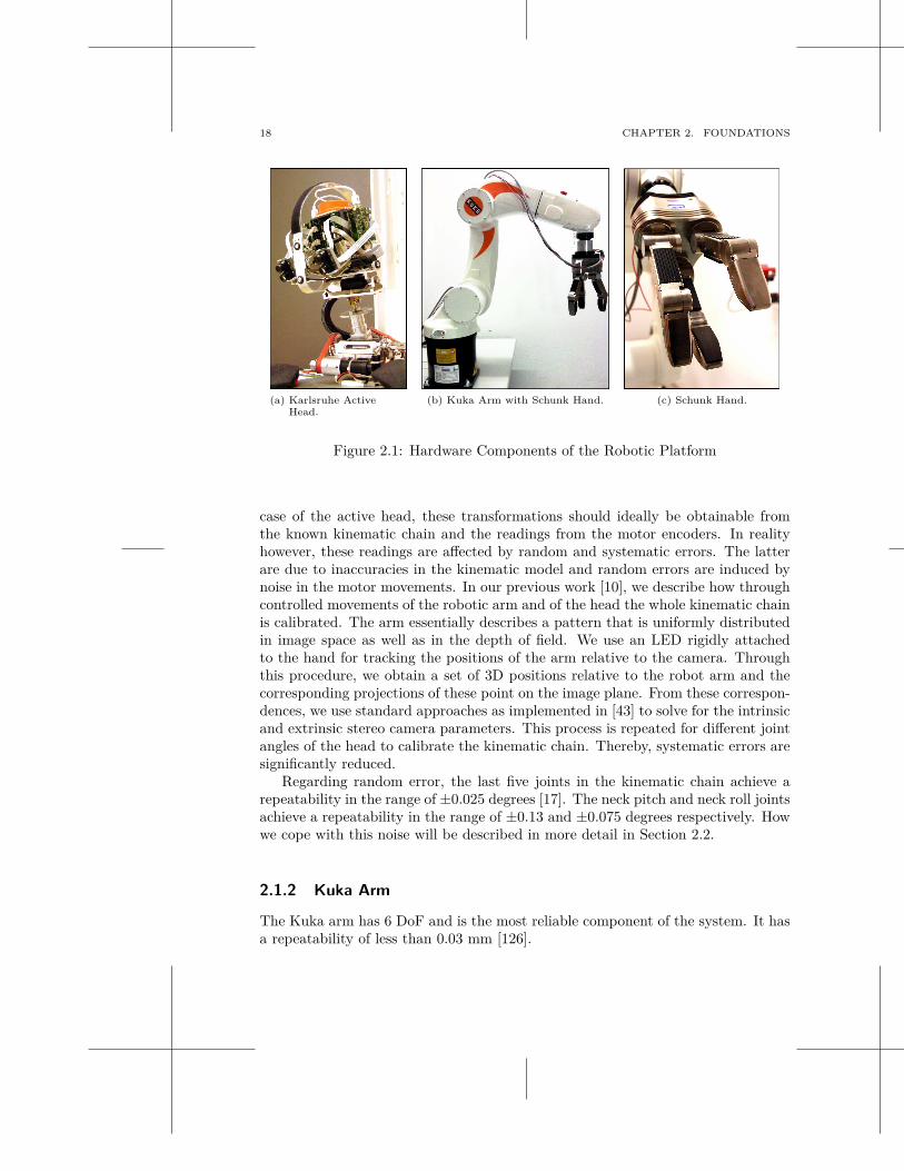
The main components of the robotic platform used throughout this thesis are theKarlsruhe active head [17] and a Kuka arm [126] equipped with a Schunk DexterousHand 2.0 (SDH) [203] as shown in Figure 2.1. This embodiment enables the robotto perform a number of actions like saccading, fixating, tactile exploration andgrasping.
2.1.1 Karlsruhe Active Head
We are using a robotic head [17] that has been developed as part of the ArmarIII humanoid robot as described in Asfour et al. [16]. It actively explore the en-vironment through gaze shifts and fixation on objects. The head has 7 DoF. Forperforming gaze shift, the lower pitch, yaw, roll as well as the eye pitch are used.The upper pitch is kept static. To fixate, the right and left eye yaw are actuatedin a coupled manner. Therefore, only 5DoF are effectively used.
The head is equipped with two stereo camera pairs. One has a focal lengthof 4mm and therefore a wide field of view. The other one has a focal length of12mm providing the vision system with a close up view of objects in the scene. Forexample images, see Figure 2.2.
To model the scene accurately from stereo measurements, the relation betweenthe two camera systems as well as between the cameras and the head origin needsto be determined after each head movement. This is different from stereo cam-eras with a static epipolar geometry that need to be calibrated only once. In the
17
18 CHAPTER 2. FOUNDATIONS
(a) Karlsruhe ActiveHead.
(b) Kuka Arm with Schunk Hand. (c) Schunk Hand.
Figure 2.1: Hardware Components of the Robotic Platform
case of the active head, these transformations should ideally be obtainable fromthe known kinematic chain and the readings from the motor encoders. In realityhowever, these readings are affected by random and systematic errors. The latterare due to inaccuracies in the kinematic model and random errors are induced bynoise in the motor movements. In our previous work [10], we describe how throughcontrolled movements of the robotic arm and of the head the whole kinematic chainis calibrated. The arm essentially describes a pattern that is uniformly distributedin image space as well as in the depth of field. We use an LED rigidly attachedto the hand for tracking the positions of the arm relative to the camera. Throughthis procedure, we obtain a set of 3D positions relative to the robot arm and thecorresponding projections of these point on the image plane. From these correspon-dences, we use standard approaches as implemented in [43] to solve for the intrinsicand extrinsic stereo camera parameters. This process is repeated for different jointangles of the head to calibrate the kinematic chain. Thereby, systematic errors aresignificantly reduced.
Regarding random error, the last five joints in the kinematic chain achieve arepeatability in the range of ±0.025 degrees [17]. The neck pitch and neck roll jointsachieve a repeatability in the range of ±0.13 and ±0.075 degrees respectively. Howwe cope with this noise will be described in more detail in Section 2.2.
2.1.2 Kuka Arm
The Kuka arm has 6 DoF and is the most reliable component of the system. It hasa repeatability of less than 0.03 mm [126].

2.2. VISION COMPONENTS 19
Reconstruction
Segmentation
StereoMatching
Fixation
Attention
Visual Front End
Images
ControlSignals
Robot Head Scene ModelReal Scene
Figure 2.2: Overview of the Input and Output of the Visual Front End. Left) Fovealand Peripheral Images of a Scene. Middle Left) Karlsruhe Active Head. MiddleRight) Visual Front End. Right) Segmented 3D Point Cloud.
2.1.3 Schunk Dexterous Hand
The SDH has three fingers each with two joints. An additional degree of freedomexecutes a coupled rotation of two fingers around their roll axis. Each finger ispadded with two tactile sensor arrays: one on the distal phalanges with 6 × 13 − 10cells and one on the proximal phalanges with 6 × 14 cells [203].
2.2 Vision Components
As input to all the methods that are proposed in this thesis, we expect a 3D pointcloud of the scene. To produce such a representation, we use a real-time activevision system running on the Karlsruhe active head. In the following, we willintroduce this system and present two different ways in which this representationis segmented into background and several object hypotheses.
2.2.1 Real-Time Vision System
In Figure 2.2, we show the structure of the real-time vision system that is capableof gaze shifts and fixation. Segmentation is tightly embedded into this system.In the following, we will briefly explain all the components. For a more detaileddescription, we refer to Rasolzadeh et al. [182], Björkman and Kragic [35], Björkmanand Eklundh [33].
20 CHAPTER 2. FOUNDATIONS
2.2.1.1 Attention
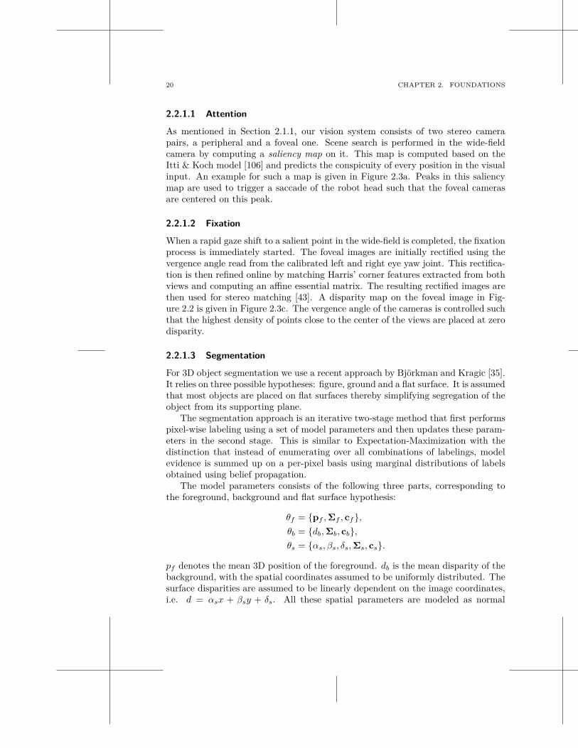
As mentioned in Section 2.1.1, our vision system consists of two stereo camerapairs, a peripheral and a foveal one. Scene search is performed in the wide-fieldcamera by computing a saliency map on it. This map is computed based on theItti & Koch model [106] and predicts the conspicuity of every position in the visualinput. An example for such a map is given in Figure 2.3a. Peaks in this saliencymap are used to trigger a saccade of the robot head such that the foveal camerasare centered on this peak.
2.2.1.2 Fixation
When a rapid gaze shift to a salient point in the wide-field is completed, the fixationprocess is immediately started. The foveal images are initially rectified using thevergence angle read from the calibrated left and right eye yaw joint. This rectifica-tion is then refined online by matching Harris’ corner features extracted from bothviews and computing an affine essential matrix. The resulting rectified images arethen used for stereo matching [43]. A disparity map on the foveal image in Fig-ure 2.2 is given in Figure 2.3c. The vergence angle of the cameras is controlled suchthat the highest density of points close to the center of the views are placed at zerodisparity.
2.2.1.3 Segmentation
For 3D object segmentation we use a recent approach by Björkman and Kragic [35].It relies on three possible hypotheses: figure, ground and a flat surface. It is assumedthat most objects are placed on flat surfaces thereby simplifying segregation of theobject from its supporting plane.
The segmentation approach is an iterative two-stage method that first performspixel-wise labeling using a set of model parameters and then updates these param-eters in the second stage. This is similar to Expectation-Maximization with thedistinction that instead of enumerating over all combinations of labelings, modelevidence is summed up on a per-pixel basis using marginal distributions of labelsobtained using belief propagation.
The model parameters consists of the following three parts, corresponding tothe foreground, background and flat surface hypothesis:
θf = {pf , Σf , cf },
θb = {db, Σb, cb},
θs = {αs, βs, δs, Σs, cs}.
pf denotes the mean 3D position of the foreground. db is the mean disparity of thebackground, with the spatial coordinates assumed to be uniformly distributed. Thesurface disparities are assumed to be linearly dependent on the image coordinates,i.e. d = αsx + βsy + δs. All these spatial parameters are modeled as normal
2.2. VISION COMPONENTS 21
distributions, with Σf , Σb and Σs being the corresponding covariances. The lastthree parameters, cf , cb and cs, are represented by color histograms expressed inhue and saturation space.
For initialization, there has to be some prior assumption of what is likely tobelong to the foreground. In this thesis, we have a fixating system and assume thatpoints close to the center of fixation are most likely to be part of the foreground.An imaginary 3D ball is placed around this fixation point and everything within theball is initially labeled as foreground. For the flat surface hypothesis, RANSAC [80]is applied to find the most likely plane. The remaining points are initially labeledas background points.
Other approaches to initializing new foreground hypotheses for example throughhuman-robot dialogue or motion of objects induced bei either a person or the robotitself are presented in [28, 29, 140]. Furthermore, these articles present the exten-sion of the segmentation framework to keep multiple object hypotheses segmentedsimultaneously.
2.2.1.4 Re-Centering
The attention points that are peaks in the saliency map on wide-field images, tend tobe on the border of objects rather than on their center. Therefore, when performinga gaze shift, the center of the foveal images does not necessarily correspond to thecenter of the objects. We perform a re-centering operation to maximize the amountof an object visible in the foveal cameras. This is done by letting the iterativesegmentation process stabilize for a specific gaze direction of the head. Then thecenter of mass of the segmentation mask is computed. A control signal is sent to thehead to correct its gaze direction such that the center of the foveal images is alignedwith the center of segmentation. After this small gaze-shift has been performed,the fixation and segmentation process are re-started. This process is repeated untilthe center of the segmentation mask is sufficiently aligned with the center of theimages.
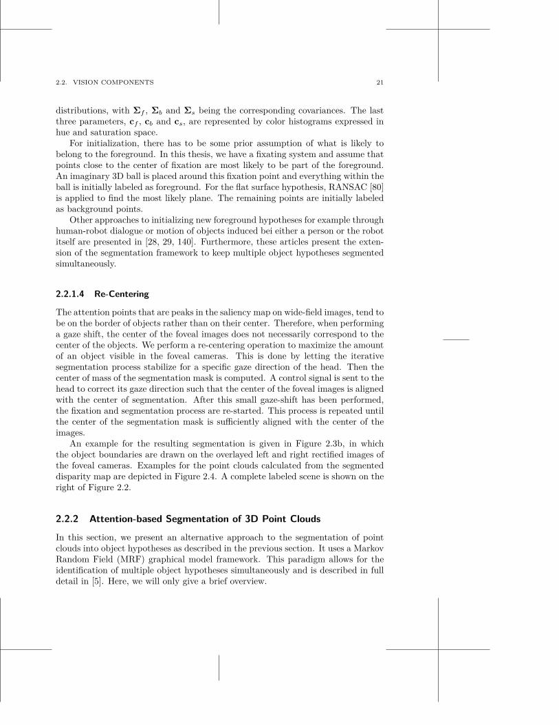
An example for the resulting segmentation is given in Figure 2.3b, in whichthe object boundaries are drawn on the overlayed left and right rectified images ofthe foveal cameras. Examples for the point clouds calculated from the segmenteddisparity map are depicted in Figure 2.4. A complete labeled scene is shown on theright of Figure 2.2.
2.2.2 Attention-based Segmentation of 3D Point Clouds
In this section, we present an alternative approach to the segmentation of pointclouds into object hypotheses as described in the previous section. It uses a MarkovRandom Field (MRF) graphical model framework. This paradigm allows for theidentification of multiple object hypotheses simultaneously and is described in fulldetail in [5]. Here, we will only give a brief overview.
22 CHAPTER 2. FOUNDATIONS
(a) Saliency Map of WideField Image.
(b) Segmentation on OverlayedFixated Rectified Left andRight Images.
(c) Disparity Map.
Figure 2.3: Example Output for Visual Processes run on Wide-Field and FovealImages shown in Figure 2.2
(a) Point Cloud of a Toy Tiger (b) Point Cloud of Mango Can
Figure 2.4: Example 3D Point Cloud (from two Viewpoints) generated from Dis-parity Map and Segmentation as shown in Figure 2.3c and 2.3b.
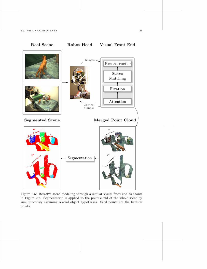
The active humanoid head uses saliency to direct its gaze. By fully reconstruct-ing each stereo view after each gaze shift and merging these resulting partial pointclouds into one, we obtain scene reconstructions as shown in Figure 2.5. The fixa-tion points serve as seed points that we project into the point cloud to create initialclusters for the generation of object hypotheses.
For full segmentation we perform energy minimization in a multi-label MRF.We use the multi-way cut framework as proposed in Boykov et al. [41]. In ourapplication, the MRF is modelled as a graph with two sets of costs for assigning aspecific label to a node in that graph: unary costs and pairwise costs.
In our case, the unary cost describes the likelihood of membership to an objecthypothesis’ color distribution. This distribution is modelled by Gaussian MixtureModels (GMMs) as utilized in GrabCuts by Rother et al. [188]. For each salientregion one GMM is created to model the color properties of that object hypothesis.
Pairwise costs enforce smoothness between adjacent labels. The pairwise struc-ture of the graph is derived from a KD-tree neighborhood search directly on thepoint cloud. The 3D structure provides the links between points and enforces neigh-
2.2. VISION COMPONENTS 23
Reconstruction
StereoMatching
Fixation
Attention
Visual Front End
Images
ControlSignals
Robot Head
Merged Point CloudSegmented Scene
Real Scene
Segmentation
Figure 2.5: Iterative scene modeling through a similar visual front end as shownin Figure 2.2. Segmentation is applied to the point cloud of the whole scene bysimultaneously assuming several object hypotheses. Seed points are the fixationpoints.
24 CHAPTER 2. FOUNDATIONS
bor consistency. Once the pairwise and unary costs are computed, the energy min-imization can be performed using standard methods. The α-expansion algorithmwith available implementation [42, 119, 40] efficiently computes an approximatesolution that approaches the NP-hard global solution.
There are several differences of this approach from the one presented in Sec-tion 2.2.1.3. First of all, no flat surface hypothesis is explicitly introduced. Thisapproach is therefore independent of the presence of a table plane. Secondly, objecthypotheses are represented by GMMs instead of color histograms and distributionsof disparities. And thirdly, several object hypotheses are segmented simultaneously.This has been shown in [5] to be beneficial for segmentation accuracy over just keep-ing one object hypothesis especially in complex scenes. However, the approach isnot real-time. Recently, the previous approach to segmentation has been extendedto simultaneously keep several object hypotheses segmented by Bergström et al.[29].
2.3 Discussion
In this chapter, we presented the hardware and software foundations used in thisthesis. They enable the robot to visually explore a scene and segment objects fromthe background as well as from each other. Furthermore, the robot can interactwith the scene with its arm and hand.
Given these capabilities, what are the remaining factors that render the problemof robust grasping and manipulation in the scene difficult? First of all, the scenemodel that is the result of the vision components is only a partial representationof the real scene. As can be observed in Figure 2.5, it has gaps and contains noise.The segmentation of objects might also be erroneous if objects of similar appearanceare placed very close to each other. Secondly, given such an uncertain scene modelit is not clear how to infer the optimal grasp pose of the arm and hand such thatsegmented objects can be grasped successfully. And lastly, the execution of a graspis subject to random and systematic error originating from noise in the motors oran imprecise model of the hardware kinematics and relation between cameras andactuators.
In the following, we will propose different methods to (i) improve scene under-standing, (ii) infer grasp poses under significant uncertainty and (iii) demonstraterobust grasping through closed-loop execution.
3
Active Scene Understanding
The term scene understanding is very general and means different things dependenton the scale of the scene, the kind of sensory data, the current task of the intelligentagent and the available prior knowledge. In the computer vision community, itrefers to the ultimate goal of being able to parse an image (usually monocular),outline the different objects or parts in it and finally label them semantically. Afew recent examples for approaches towards this goal are presented by Liu et al.[137], Malisiewicz and Efros [143] and Li et al. [134]. Their common denominatoris the reliance on labeled image databases on which for example similarity metricsor category models are learnt.
In the robotics community the goal of scene understanding is similar, however,the prerequisites for achieving it are different. First, a robot is an embodied systemthat cannot only move in the environment but also interact with it and therebychange it. And second, robotic platforms are usually equipped with a whole sensorsuite delivering multi-modal observations of the environment, e.g., laser range data,monocular or stereo images and tactile sensor readings. Depending on the researcharea, the task of scene understanding changes. In mobile robotics, the scene canbe an office floor or even a whole city. The aim is to acquire maps suitable fornavigation, obstacle avoidance and planning. This map can be metric as for examplein O’Callaghan et al. [162] and Gallup et al. [85]; it can use topological structuresfor navigation as in Pronobis and Jensfelt [178] and Ekvall et al. [71] or it cancontain semantic information as for example in Wojek et al. [232] and Topp [220].Pronobis and Jensfelt [178], Ekvall et al. [71] and Topp [220] combine these differentrepresentations into a layered architecture. The metric map constitutes the mostdetailed and therefore bottommost layer. The higher up a layer in this architecture,the more abstracted it is from the metric map.
If the goal is mobile manipulation, the requirements for the maps change. Moreemphasis has to be placed on the objects in the scene that have to be manipulated.These objects can be doors as for example in Rusu et al. [196], Klingbeil et al. [117]and Petersson et al. [170] but also items we commonly find in our offices and homeslike cups, books or toys as shown for example in Kragic et al. [122], Ciocarlie et al.[52], Grundmann et al. [95] and Marton et al. [148]. Approaches towards mobilemanipulation mostly differ in what kind of prior knowledge is assumed. This ranges
25
26 CHAPTER 3. ACTIVE SCENE UNDERSTANDING
from full CAD models of objects to very low level heuristics for grouping 3D pointsinto clusters. A more detailed review on these will be presented in Chapter 7.
Other approaches towards scene understanding exploit the capability of a robotto interact with the scene. Bergström et al. [28] and Katz et al. [110] use motioninduced by a robot to segment objects from each other or to learn kinematic modelof articulated objects. Luo et al. [140] and Papadourakis and Argyros [164] segmentdifferent objects from each other by observing a person interacting with them.
An insight that can be derived from these very different approaches towardsscene understanding is that there is yet no representation that has been widelyadopted across different areas in robotics. The choice is usually made dependenton task, available sensor data and scale of the scene.
A common situation in robotics is that the scene cannot be captured completelyin one view. Instead, several subsequent observations are merged. The task of therobot usually determines what parts of the environment are currently interestingand what parts are irrelevant. Hence, it is desirable for the robot to adopt anexploration strategy that accelerates the understanding of the task-relevant detailsof the scene as opposed to exhaustively examining its whole surroundings.
The research field of active perception as defined by Bajcsy [20] is concernedwith planning a sequence of control strategies that minimise a loss function whileat the same time maximise the amount of obtained information. Especially inthe field of active vision, this paradigm has led to the development of head-eyesystems as in Ballard [22] and Pahlavan and Eklundh [163]. They could shift theirgaze and fixate on task-relevant details of the scene It was shown that throughthis approach, visual computation of task-relevant representations could be madesignificantly more efficient. The active vision system utilized in this thesis is basedon the findings in Rasolzadeh et al. [182]. As described in Section 2.2.1, it exploresa scene guided by an attention system. The resulting high resolution detail of thescene is then used to grasp objects. Other examples for active vision systems arethose concerned with view planning for object recognition like for example Roy[190] or reconstruction like Wenhardt et al. [230]. Aydemir et al. [18] applied activesensing strategies for efficiently searching for objects in large scale environments.
Problem Formulation In the following three chapters of this thesis, we studythe problem of scene understanding for grasping and manipulation in the presenceof multiple instances of unknown objects. The scenes considered here will be thevery common case of table-top environments. We are considering different sourcesof information that will help us with this task. These can be sensors such as thevision system and tactile arrays described in Section 2.1 or they can be humansthat the robot is interacting with through a dialog system.
Requirements The proposed methods have to be able to integrate multi-modalinformation into a unified scene representation. They have to be robust to noise toestimate an accurate model of the scene suitable for grasping and manipulation.
27
Assumptions Throughout most of this thesis, we make the common assumptionthat the dominant plane in the scene can be detected. As already noted by Ballard[22], this kind of context information allows to constrain different optimisationproblems or allow for an efficient scene representation. However, we will discusshow the proposed methods are affected when no dominant plane can be detectedand how they could be generalized to this case.
We bootstrap the scene understanding process through obtaining an initiallysegmented scene model from the active vision system. First object hypotheses willbe already segmented from the background as visualized in Figure 2.2.
Throughout most of these next three chapters of the thesis, we are assuming thatwe do not have any prior knowledge on specific object instances or object categories.Instead, we start from assumptions about objectness, i.e., general characteristics ofwhat an object constitutes. A commonly used assumption is that objects tend tobe homogeneous in their attribute space. The segmentation methods described inSection 2.2.1.3 use color and disparity as these attributes to group specific locationsin the visual input to object hypotheses. Other characteristics can be general objectshape as for example symmetry.
Approach As emphasized by Bajcsy [20], prediction is essential in active percep-tion. Without being able to predict the outcome of specific actions, neither theircost nor their benefit can be computed. Hence, the information for choosing thebest sequence of actions is missing.
To enable prediction, sensors and actuators as well as their interaction has tobe modelled with minimum error. Consider for example, the control of the activestereo head in Figure 2.1a. If we had no model of its forward kinematics, we wouldnot be able to predict the direction in which the robot is going to look after sendingcommands to the motors.
Modeling the noise profiles of the system components also gives us an idea aboutthe uncertainty of the prediction. For example, we are using the haptic sensors ofour robotic hand for contact detection. By modeling the noise profile of the sensorpads, we can quantify the uncertainty in each contact detection.
In the following chapters, we will propose different implementations of the func-tion g(·) in Equation 1.1 to make predictions about parts of the scene that havenot been observed so far:
x+t = g(xt)
in which the current estimate xt of the state of the scene is predicted to be x+t .
Additionally we are also interested in quantifying how uncertain we are about thisprediction, i.e., in the associated variance Σ+
t . We will study different models of thescene state x but also different kinds of assumptions and priors about objectness.These will have different implications on what can be predicted and how accurate.The resulting predictions will help to guide active exploration of the scene, toupdate the current scene model and to interact with it in a robust manner.
28 CHAPTER 3. ACTIVE SCENE UNDERSTANDING
In Chapter 4, we will use the framework of Gaussian Processes (GP) to predictthe geometric structure of a whole table top scene and guide haptic exploration.The state x is modelled as a set of 2D locations xi = (ui, vi)T on the table. In thischapter, we are studying two different scene representations and their applicabilityto the task of grasping and manipulation. In an occupancy grid, each location has avalue indicating its probability p(xi = occ|{z}t) to be occupied by an object giventhe set of observations {z}t. In a height map, each location has a value that isequal to the height hi of the object standing on it. Using the GP framework, weapproximate the function g(·) by a distribution g(xt) ∼ N (µ, Σ) where x+
t = µ andΣ+
t = Σ. As will be detailed in Chapter 4, this distribution is computed given aset of sample observations and a chosen covariance function. This choice imposesa prior on the kind of structure that can be estimated.
In Chapter 5, we explore how a person interacting through a dialogue systemcan help a robot in improving its understanding of the scene. We assume thatan initial scene segmentation is given by the vision system in Section 2.2. Thestate of the scene x is modelled as a set of 3D points xi = (xi, yi, zi)T . These arecarrying labels li which indicate whether they belong to the background (li = 0)or to one of N object hypotheses (li = j with j ∈ 1 . . . N). In this chapter,we are specifically dealing with the case of an under-segmentation of objects thatcommonly happens when applying a bottom-up segmentation technique to objectsof similar appearance standing very close to each other. We utilise the observationthat single objects tend to be more uniform in certain attributes than two objectsthat are grouped together. Given this prior, a set of points {x}j that are assumedto belong to an object hypothesis j and a feature vector zj , we can estimate theprobability p({x}j = j|zj) of the set to belong to one object hypothesis j. If thisestimate falls below a certain threshold, disambiguation is triggered with the helpof a human operator. Based on this information, the function g(·) improves thecurrent segmentation of the scene by re-estimating the labels of each scene point.
In Chapter 6, we focus on single object hypotheses rather than on whole scenestructures. We show how we can predict the complete geometry of unknown objectsto improve grasp inference. As in the previous chapter, the state of the scene ismodelled as a set of 3D points xi = (xi, yi, zi)T and we want to estimate whichones belong to a specific object hypothesis. Different to the previous section, ourgoal is not to re-estimate the labels of observed points. Instead, the function g(·)has to add points to the scene that are assumed to belong to an object hypothesis.As a prior, we assume that especially man-made objects are commonly symmetric.The problem of modeling the unobserved object part can then be formulated as anoptimisation of the parameters of the symmetry plane. The uncertainty about eachadded point is computed based on visibility constraints.
4
Predicting and Exploring Scenes
The ability to interpret the environment, detect and manipulate objects is at theheart of many autonomous robotic systems as for example in Petersson et al. [170]and Ekvall et al. [71]. These systems need to represent objects for generating task-relevant actions. In this chapter, we present strategies for autonomously exploringa table-top scene. Our robotic setup consists of the vision system presented inSection 2.2 that generates initial object hypotheses using active visual segmentation.Thereby, large parts of the scene are explored in a few glances. However, withoutsignificantly changing the viewpoint, areas behind objects are occluded. For findingsuitable grasp or for deciding where to place an object once it is picked up, adetailed representation of the scene in the current radius of interaction is essential.To achieve this, parts of the scene that are not visible to the vision system areactively explored by the robot using its hand with tactile sensors. Compared to agaze shift, moving the arm is expensive in terms of time and gain in information.Therefore, the next best measurement has to be determined to explore the unknownspace efficiently.
In this chapter, we study different aspects of this problem. First of all, weneed to find an accurate and efficient scene representation that can accomodatemulti-modal information. In Section 4.1 and 4.2, we analyse the feasibility of anoccupancy grid and a height map for grasping and manipulation.
Second, we need to find efficient exploration strategies that provide maximuminformation at minimum cost. We compare two approaches from the area of mobilerobotics. First, we use Spanning Tree Covering (STC) as proposed by Gabriely andRimon [83]. It is optimal in the sense that every place in the scene is explored justonce. Secondly, we extend the approach presented in O’Callaghan et al. [162] whereunexplored areas are predicted from sparse sensor measurements by a GaussianProcess (GP). Exploration then aims at confirming this prediction and reducing itsuncertainty with as few sensing actions as possible.
The resulting scene model is multi-modal in the sense that it i) generates objecthypotheses emerging from the integration of several visual cues, and ii) fuses visualand haptic information.
29
30 CHAPTER 4. PREDICTING AND EXPLORING SCENES
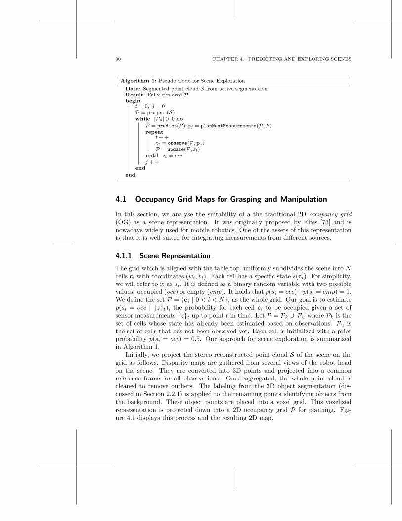
Algorithm 1: Pseudo Code for Scene Exploration
Data: Segmented point cloud S from active segmentationResult: Fully explored Pbegin
t = 0, j = 0P = project(S)while |Pu| > 0 do
P = predict(P) pj = planNextMeasurements(P, P)repeat
t + +zt = observe(P, pj)P = update(P, zt)
until zt 6= occj + +
end
end
4.1 Occupancy Grid Maps for Grasping and Manipulation
In this section, we analyse the suitability of a the traditional 2D occupancy grid(OG) as a scene representation. It was originally proposed by Elfes [73] and isnowadays widely used for mobile robotics. One of the assets of this representationis that it is well suited for integrating measurements from different sources.
4.1.1 Scene Representation
The grid which is aligned with the table top, uniformly subdivides the scene into Ncells ci with coordinates (wi, vi). Each cell has a specific state s(ci). For simplicity,we will refer to it as si. It is defined as a binary random variable with two possiblevalues: occupied (occ) or empty (emp). It holds that p(si = occ)+p(si = emp) = 1.We define the set P = {ci | 0 < i < N}, as the whole grid. Our goal is to estimatep(si = occ | {z}t), the probability for each cell ci to be occupied given a set ofsensor measurements {z}t up to point t in time. Let P = Pk ∪ Pu where Pk is theset of cells whose state has already been estimated based on observations. Pu isthe set of cells that has not been observed yet. Each cell is initialized with a priorprobability p(si = occ) = 0.5. Our approach for scene exploration is summarizedin Algorithm 1.
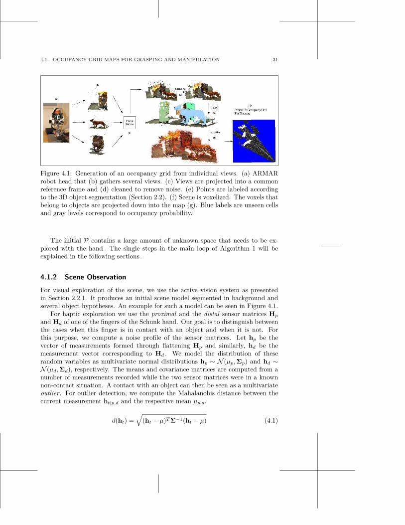
Initially, we project the stereo reconstructed point cloud S of the scene on thegrid as follows. Disparity maps are gathered from several views of the robot headon the scene. They are converted into 3D points and projected into a commonreference frame for all observations. Once aggregated, the whole point cloud iscleaned to remove outliers. The labeling from the 3D object segmentation (dis-cussed in Section 2.2.1) is applied to the remaining points identifying objects fromthe background. These object points are placed into a voxel grid. This voxelizedrepresentation is projected down into a 2D occupancy grid P for planning. Fig-ure 4.1 displays this process and the resulting 2D map.
4.1. OCCUPANCY GRID MAPS FOR GRASPING AND MANIPULATION 31
Figure 4.1: Generation of an occupancy grid from individual views. (a) ARMARrobot head that (b) gathers several views. (c) Views are projected into a commonreference frame and (d) cleaned to remove noise. (e) Points are labeled accordingto the 3D object segmentation (Section 2.2). (f) Scene is voxelized. The voxels thatbelong to objects are projected down into the map (g). Blue labels are unseen cellsand gray levels correspond to occupancy probability.
The initial P contains a large amount of unknown space that needs to be ex-plored with the hand. The single steps in the main loop of Algorithm 1 will beexplained in the following sections.
4.1.2 Scene Observation
For visual exploration of the scene, we use the active vision system as presentedin Section 2.2.1. It produces an initial scene model segmented in background andseveral object hypotheses. An example for such a model can be seen in Figure 4.1.
For haptic exploration we use the proximal and the distal sensor matrices Hp
and Hd of one of the fingers of the Schunk hand. Our goal is to distinguish betweenthe cases when this finger is in contact with an object and when it is not. Forthis purpose, we compute a noise profile of the sensor matrices. Let hp be thevector of measurements formed through flattening Hp and similarly, hd be themeasurement vector corresponding to Hd. We model the distribution of theserandom variables as multivariate normal distributions hp ∼ N (µp, Σp) and hd ∼N (µd, Σd), respectively. The means and covariance matrices are computed from anumber of measurements recorded while the two sensor matrices were in a knownnon-contact situation. A contact with an object can then be seen as a multivariateoutlier . For outlier detection, we compute the Mahalanobis distance between thecurrent measurement ht|p,d and the respective mean µp,d.
d(ht) =√
(ht − µ)T Σ−1(ht − µ) (4.1)
32 CHAPTER 4. PREDICTING AND EXPLORING SCENES
Note that the subscripts p and d are skipped in this equation for simplicity. If d(ht)is greater than a threshold φ, then we know that this haptic sensor matrix is incontact and zt = contact. Otherwise, zt = ¬contact.
4.1.3 Map Update
For each movement of the haptic sensors along the planned path, we are receivinga measurement zt+1. Based on this and the current estimate p(si = occ | {z}t) ofthe state of each cell si in the occupancy grid, we want to estimate
p(si = occ | {z}t+1) =p(zt+1 | si = occ) p(si = occ | {z}t)
∑
sip(zt+1 | si)p(si | {z}t)
(4.2)
In this recursive formulation, the resulting new estimate p(si = occ | {z}t+1) isstored in the occupancy grid. p(zt+1 | si) constitutes the haptic sensor model. Tocompute p(zt+1 | si = emp), the current measurement ht+1|p,d and Equation 4.1 isused as follows
p(zt+1 | si = emp) = exp(−12
d(ht+1)) (4.3)
= exp(−12
√
(ht+1 − µ)T Σ−1(ht+1 − µ)) (4.4)
For the case si = occ, we empirically determined the following discrete proba-bility values
p(zt+1 = contact | si = occ) = 0.9 (4.5)
p(zt+1 = ¬contact | si = occ) = 1 − p(zt+1 = contact | si = occ). (4.6)
An alternative to this way of modeling the sensor response (when in contact withan object) is to collect a set of measurements. From this set a distribution couldbe estimated similar to what is described in Section 4.1.2. However, given themany different shapes of objects and the resulting variety of haptic sensor patterns,modeling the opposite case of a non-contact is the simpler but still effective solution.
4.1.4 Map Prediction
In the traditional occupancy grid, cells that have not been observed yet will have aprobability p(si = occ | {z}t) = 0.5, i.e. there is no information available about thestate of these cells. However, we know that cells in the grid that are close to occupiedspaces but are due to occlusions not directly observable, are likely to be part of theoccluding object. By modeling this spatial correlation, we can predict unobservedplaces from observed ones. Instead of exploring the whole environment exhaustively,we want to confirm the predicted map at specifically uncertain places. Recently,O’Callaghan et al. [162] proposed that the spatial correlation in a 2D occupancy
4.1. OCCUPANCY GRID MAPS FOR GRASPING AND MANIPULATION 33
grid can be modeled with a Gaussian Process. The assumption of independence ofneighboring cells in traditional occupancy grids is removed.
A GP is used to fit a likelihood function to training data. In our case this is theset of cells cr ∈ Pk and their estimated state sr of occupancy. Given the estimatedcontinuous function over the occupancy grid, we can then estimate the state sj ofthe cells cj ∈ Pu that have not been observed yet. We will briefly introduce GPsfirst for the simpler case of regression and then for the problem of classifying a cellto be either occupied or empty which is the core of this section. For a more detailedexplanation, we refer to Rasmussen and Williams [181].
4.1.4.1 Gaussian Process Regression
A GP is defined as a collection of a finite number of random variables with a jointGaussian distribution. A GP can be seen as a distribution over functions with amean µ and covariance Σ. Given a set of input values x and corresponding targetvalues y, the goal in GP regression is to estimate the underlying latent function g(·)that generated these samples. We will also refer to the set {xi, yi}M as the trainingset with cardinality M . Expressed as a linear regression model with Gaussian noiseǫ, the relation between input and target values can be modelled as follows:
g(xi) = φ(xi)T w, yi = g(xi) + ǫ (4.7)
with the noiseǫ ∼ N (0, σ2
M ) (4.8)
following an independently and identically distributed Gaussian with zero meanand variance σ2
M . w is a vector of weight parameters of the linear model. φ(xi)is a function that maps D-dimensional input data into an N -dimensional featurespace. Under this formulation, the likelihood of the training data given the modelis computed as a factored distribution over all training samples:
p(y|x, w) =M∏
i=1
p(yi|xi, w) (4.9)
=M∏
i=1
1√2πσM
exp(− (yi − φ(xi)T w)2σ2
M
) (4.10)
= N(φ(x)T w, σ2M I). (4.11)
If we use a zero-mean Gaussian prior on the weights w ∼ N (0, Σw), then theposterior likelihood p(w|x, y) is proportional to the product of the likelihood andthe prior
p(w|x, y) ∝ p(y|x, w)p(w) (4.12)
which is again Gaussian.We are primarily interested in predicting the target value y′ for new input
values x′. The predictive distribution p(g(x′)|x′, x, y) is computed by averaging
34 CHAPTER 4. PREDICTING AND EXPLORING SCENES
the outputs of all possible linear models weighted with the posterior distribution ofthe model given the training set:
p(g(x′)|x′, x, y) =∫
p(g(x′)|x′, w)p(w|x, y)dw. (4.13)
Since all the factors over which we want to integrate follow a Gaussian distri-bution, we can evaluate the integral in Equation 4.13 analytically. The predictivedistribution is then Gaussian again and defined as g(x′) ∼ N (µ, Σ) where
µ = k(x′, x)T [K(x, x) + σ2M I]−1y (4.14)
Σ = k(x′, x′) − k(x′, x)T [K(x, x) + σ2M I]−1k(x′, x). (4.15)
The entries of the Gram matrix K(x, x)a,b at row a and column b are definedbased on a covariance function k(xa, xb) with some hyperparameters θ and witha, b ∈ {1 . . . M}. This covariance function is related to the function φ(·) fromEquation 4.7 as follows:
k(xa, xb) = φ(xa)T Σw φ(xb). (4.16)
The most widely used covariance function is the squared exponential (SE)
k(xa, xb) = σ2l exp(−((xa − xb)T L−1(xa − xb))/2) (4.17)
where the hyperparameters are σl, the signal variance, and L, the identity matrixmultiplied with the length scale l. There is a large set of other covariance functionsproposed in the literature. More details about those applied in this thesis can befound in Appendix A. As will be shown later in Section 4.1.6, the simple SE kernelachieves the best results for scene prediction during exploration.
The kind of covariance function as well as its hyperparameters have to be chosensuch that g(·) optimally models the underlying process. As suggested in [181],this model selection problem can be treated in a Bayesian way. In this thesis,we want to choose the hyperparameters of a given covariance function such thatthe marginal likelihood p(y|x, θ) of the data given the model is maximised. Thismarginal likelihood is defined as follows:
p(y|x, θ) =∫
p(y|x, f , θ)p(f |x)df (4.18)
where f = g(x). A desirable property of p(y|x, θ) is that it automatically tradesoff model fit against model complexity. This can be observed when writing out thelogarithm of the marginal likelihood. The integral can be computed analyticallysince both, the prior and the likelihood in Equation 4.18 are Gaussian:
log p(y|x, θ) = −12
yT K−1y − 12
log |K| − M
2log 2π (4.19)
4.1. OCCUPANCY GRID MAPS FOR GRASPING AND MANIPULATION 35
where K is short hand for K(x, x)+σ2M I. The first part of the sum in Equation 4.19
reflects how well the data fits the model. The second part penalizes model com-plexity and is only dependent on the covariance function and its input. The lastpart is a normalisation term. By equating the partial derivatives of the log marginallikelihood with respect to the hyperparameters to zero, we can solve for the optimalhyperparameters of a given covariance function and training set.
4.1.4.2 Gaussian Process Classification
Predicting the binary state of a cell in an occupancy grid is a classification ratherthan a regression problem. Our training set consists of the coordinates (w, v)r ofall the cells cr ∈ Pk as x and their observed state sr as y. This state is binary andcan be either occupied or empty. Our goal is to compute p(sj = occ | {z}t), theprobability that the state sj of a cell cj ∈ Pu is occupied. Note, that this cell hasnot been observed yet.
The basic idea behind Gaussian Process classification is very simple. Let x′ = cj
and y′ = sj , then we can compute p(y′ = occ | {z}t) by squashing the predictivedistribution g(x′) through the cumulative Gaussian function:
p(y′ = occ | {z}t) = 1/2 · (1 + erf(g(x′)/√
2)). (4.20)
However, the distribution g(x′) cannot be computed analytically as in the case ofregression where the posterior p(w|x, y) is Gaussian. For classification where thetarget values are either +1 (occupied) or −1 (empty), the likelihood p(yi|xi, w) ofa data point given the model is a sigmoid function
p(yi|xi, w) = σ(yixTi w). (4.21)
The likelihood p(y|x, w) of the whole training data will therefore be non-Gaussian.Even if we use the same prior on the weights w, the posterior as in Equation 4.12will be non-Gaussian. Therefore, calculating the predictive distribution g(x′) as inEquation 4.13, requires evaluating an integral over a non-Gaussian posterior. Dif-ferent approximations for this problem have been proposed. We follow the Laplaceapproach in which the posterior p(w|y, x) is approximated as a Gaussian.
An example for this prediction given a 2D map of partially explored scene isgiven in Figure 4.2. In Section 4.1.6, we will show quantitatively on synthetic datathat a GP predicted map is a reasonable estimate of the ground truth.
4.1.5 Action Selection for Exploration
Given a partial map of the environment, we want to efficiently explore the remain-ing unknown parts with haptic sensors, i.e., we want to minimize the amount ofmeasurement actions needed to reach a sufficient scene understanding. We willpresent two algorithms for planning a measurement path in the given map. First,we will use Spanning Tree Covering [83]. Second, we propose an active learningscheme based on the predicted map.
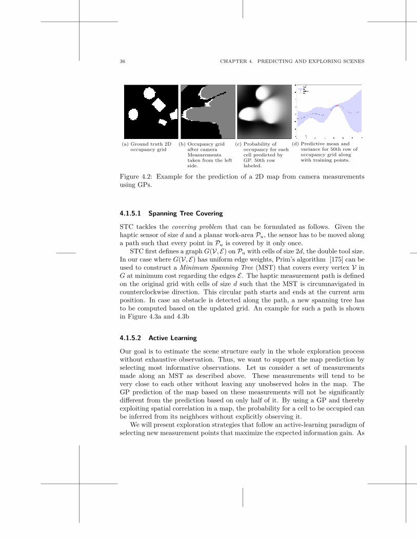
36 CHAPTER 4. PREDICTING AND EXPLORING SCENES
(a) Ground truth 2Doccupancy grid
(b) Occupancy gridafter cameraMeasurementstaken from the leftside.
(c) Probability ofoccupancy for eachcell predicted byGP. 50th rowlabeled.
(d) Predictive mean andvariance for 50th row ofoccupancy grid alongwith training points.
Figure 4.2: Example for the prediction of a 2D map from camera measurementsusing GPs.
4.1.5.1 Spanning Tree Covering
STC tackles the covering problem that can be formulated as follows. Given thehaptic sensor of size d and a planar work-area Pu, the sensor has to be moved alonga path such that every point in Pu is covered by it only once.
STC first defines a graph G(V, E) on Pu with cells of size 2d, the double tool size.In our case where G(V, E) has uniform edge weights, Prim’s algorithm [175] can beused to construct a Minimum Spanning Tree (MST) that covers every vertex V inG at minimum cost regarding the edges E . The haptic measurement path is definedon the original grid with cells of size d such that the MST is circumnavigated incounterclockwise direction. This circular path starts and ends at the current armposition. In case an obstacle is detected along the path, a new spanning tree hasto be computed based on the updated grid. An example for such a path is shownin Figure 4.3a and 4.3b
4.1.5.2 Active Learning
Our goal is to estimate the scene structure early in the whole exploration processwithout exhaustive observation. Thus, we want to support the map prediction byselecting most informative observations. Let us consider a set of measurementsmade along an MST as described above. These measurements will tend to bevery close to each other without leaving any unobserved holes in the map. TheGP prediction of the map based on these measurements will not be significantlydifferent from the prediction based on only half of it. By using a GP and therebyexploiting spatial correlation in a map, the probability for a cell to be occupied canbe inferred from its neighbors without explicitly observing it.
We will present exploration strategies that follow an active-learning paradigm ofselecting new measurement points that maximize the expected information gain. As
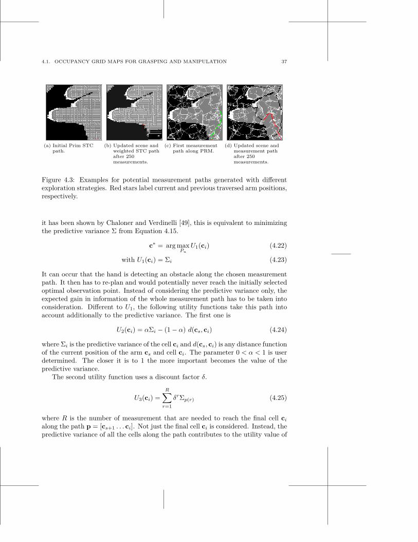
4.1. OCCUPANCY GRID MAPS FOR GRASPING AND MANIPULATION 37
(a) Initial Prim STCpath.
(b) Updated scene andweighted STC pathafter 250measurements.
(c) First measurementpath along PRM.
(d) Updated scene andmeasurement pathafter 250measurements.
Figure 4.3: Examples for potential measurement paths generated with differentexploration strategies. Red stars label current and previous traversed arm positions,respectively.
it has been shown by Chaloner and Verdinelli [49], this is equivalent to minimizingthe predictive variance Σ from Equation 4.15.
c∗ = arg maxPu
U1(ci) (4.22)
with U1(ci) = Σi (4.23)
It can occur that the hand is detecting an obstacle along the chosen measurementpath. It then has to re-plan and would potentially never reach the initially selectedoptimal observation point. Instead of considering the predictive variance only, theexpected gain in information of the whole measurement path has to be taken intoconsideration. Different to U1, the following utility functions take this path intoaccount additionally to the predictive variance. The first one is
U2(ci) = αΣi − (1 − α) d(cs, ci) (4.24)
where Σi is the predictive variance of the cell ci and d(cs, ci) is any distance functionof the current position of the arm cs and cell ci. The parameter 0 < α < 1 is userdetermined. The closer it is to 1 the more important becomes the value of thepredictive variance.
The second utility function uses a discount factor δ.
U3(ci) =R
∑
r=1
δrΣp(r) (4.25)
where R is the number of measurement that are needed to reach the final cell ci
along the path p = [cs+1 . . . ci]. Not just the final cell ci is considered. Instead, thepredictive variance of all the cells along the path contributes to the utility value of
38 CHAPTER 4. PREDICTING AND EXPLORING SCENES
STC PRM
OG Occupancy grid explored through Span-ning Tree Covering.
Occypancy grid explored through Proba-bilistic Roadmap approach.
GP Gaussian Process-based map exploredthrough Spanning Tree Covering
Gaussian Process-based map exploredthrough Probabilistic Roadmap approach
Table 4.1: Summary of scene models and exploration strategies evaluated in thissection.
ci. The parameter δ has to be chosen by the user. It steers how steep the decreaseof influence of the cells in the path are dependent on their distance from the currentarm position.
To find the global maxima of Equation 4.22 we have to maximize over all cellsci in Pu and over all the paths through which a cell can be reached from cs. Sincethis is a prohibitive number of possibilities to compute, we use sampling techniquesto find a local maxima of the utility functions. We are building a probabilistic roadmap (PRM) in the two dimensional C-space of the occupancy grid [111].
A set T of cells from P is sampled according to their predictive variance andconnected to the PRM. The Dijkstra algorithm is used to compute the shortestpath from the current arm position to each cell in T through the PRM. The resultis used to compute the utility of each cell in T . An example for the PRM andtherefore the possible paths to traverse is shown in Figure 4.3c and 4.3d.
4.1.6 Experiments
In this section, we evaluate the proposed scene models and exploration strategies.We are specifically interested in how accurate the scene estimates are when usingan occupancy grid map or a Gaussian Process based prediction. Furthermore, wewant to compare the different exploration strategies in terms of how fast an accuratescene estimate is achieved. The different combinations of scene representations andexploration methods are summarized in Table 4.1.
4.1.6.1 Synthetic Data Set
Data Set and Measure of Comparison We generated 100 different 2D occu-pancy grids (70×70 cells) of which an example appears in Figure 4.2a. Every scenecontains ten objects that can either be of circular, elliptical or rectangular shapewith a random size, aspect ratio, orientation and position. Overlapping is allowedso that fewer than ten connected components can occur as well as more complexcontours.
For every scene, we simulated three camera observations made from a fixedposition on their left side with a random direction. As a sensor model, we useda beam model with a Gaussian profile [73]. Given a measurement, the occupancy
4.1. OCCUPANCY GRID MAPS FOR GRASPING AND MANIPULATION 39
grid gets updated according to Equation 4.2. An example for the result of thissimulation is shown in Figure 4.2b.
We posed the validation problem of occupancy grid estimation as a binary clas-sification into empty or occupied cells. For each estimated grid at any time in theexploration process, the number of false and true positives can be computed fordifferent thresholds resulting in an ROC curve. For evaluating the development ofthis curve over time, we choose the area under the ROC curve (AUC) as a measure.It corresponds to the probability that the state of a cell is correctly classified.
Covariance Functions Compared O’Callaghan et al. [162] claim that theneural network covariance function is especially suitable for predicting the non-stationary behavior of a typical map data set. That data is recorded from indoorand outdoor environments either with hallways, rooms, walls or streets bounded bybuildings. However, evaluations on our experimental data showed superior perfor-mance when using the squared exponential covariance function. It poses a betterprior for scenes in which blob-like objects are spread on a table.
We predicted each of the 100 occupancy grids with a GP by sampling differ-ent numbers of training points from the space observed by the camera and thenquerying p(si = occ | {z}t) for ci ∈ Pu. We compared seven different covariancefunctions with each other. Among these are the already discussed neural networkcovariance function (NN), the squared exponential function with and without au-tomatic relevance detection (SE or SEARD), the Mátern covariance function withdifferent parameters ν (Mat) and the rational quadratic (RQ). A more detailedexplanation of these kernels can be found in Appendix A. While the SE covariancefunction is determined by only one length scale, the others expose more flexibility.For example SEARD can be parameterized in terms of its hyperparameters andadapt the length scale of each input dimension according to its detected relevancy.An RQ kernel can be seen as a scale mixture of SE kernels of different length scales.And a Mat kernel is characterized by varying degrees of smoothness.
Table 4.4 lists the classification accuracy given different kernels and number ofsamples from the free space. Since the occupied space is significantly smaller thanthe free space, we keep the number of samples from there fixed to a maximum of200 points. Points are sampled according to their confidence.
SEARD always outperforms the other kernels. For visualisation, the corre-sponding ROC curves of all kernels for 400 samples are shown in Figure 4.5a. Theyshow that the neural network kernel is clearly outperformed by all the other kernels.The difference between the remaining kernels is not large. Furthermore, Figure 4.5bshows that the number of samples from the free space does not have a significantinfluence on the classification performance.
Prediction vs Occupancy Grid An important question is whether the GPmakes a valid prediction of the scene map and how this compares to the traditionaloccupancy grid. In an OG, only those estimates for p(si = occ | {z}t) are different
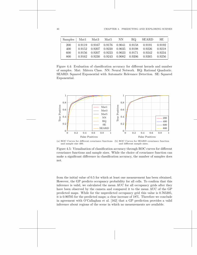
40 CHAPTER 4. PREDICTING AND EXPLORING SCENES
Samples Mat1 Mat3 Mat5 NN RQ SEARD SE
200 0.9119 0.9167 0.9176 0.9041 0.9158 0.9191 0.9192400 0.9152 0.9207 0.9220 0.9035 0.9198 0.9226 0.9218600 0.9156 0.9207 0.9223 0.9023 0.9171 0.9242 0.9234800 0.9162 0.9230 0.9243 0.9082 0.9206 0.9265 0.9256
Figure 4.4: Evaluation of classification accuracy for different kernels and numberof samples. Mat: Mátern Class. NN: Neural Network. RQ: Rational Quadratic.SEARD: Squared Exponential with Automatic Relevance Detection. SE: SquaredExponential.
0 0.2 0.4 0.6 0.8 10
0.2
0.4
0.6
0.8
1
False Positives
Tru
eP
osi
tives Mat1
Mat3
Mat5
NN
RQ
SE
SEARD
(a) ROC Curves for different covariance functionsand sample size 400.
0 0.2 0.4 0.6 0.8 10
0.2
0.4
0.6
0.8
1
False Positives
Tru
eP
osi
tives
200
400
600
800
(b) ROC Curves for SEARD covariance functionand different sample sizes.
Figure 4.5: Visualisation of classification accuracy through ROC curves for differentcovariance functions and sample sizes. While the choice of covariance function canmake a significant difference in classification accuracy, the number of samples doesnot.
from the initial value of 0.5 for which at least one measurement has been obtained.However, the GP predicts occupancy probability for all cells. To confirm that thisinference is valid, we calculated the mean AUC for all occupancy grids after theyhave been observed by the camera and compared it to the mean AUC of the GPpredicted maps. While for the unpredicted occupancy grid this value is 0.765205,it is 0.90705 for the predicted maps; a clear increase of 18%. Therefore we concludein agreement with O’Callaghan et al. [162] that a GP prediction provides a validinference about regions of the scene in which no measurements are available.
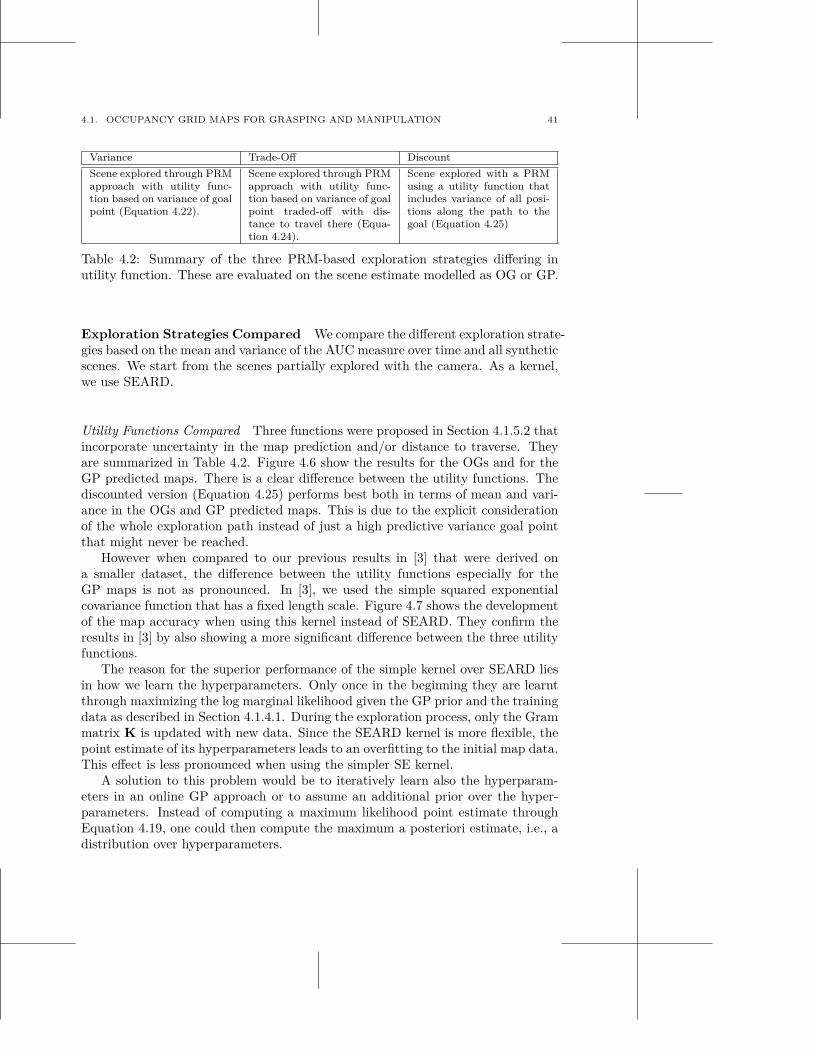
4.1. OCCUPANCY GRID MAPS FOR GRASPING AND MANIPULATION 41
Variance Trade-Off Discount
Scene explored through PRMapproach with utility func-tion based on variance of goalpoint (Equation 4.22).
Scene explored through PRMapproach with utility func-tion based on variance of goalpoint traded-off with dis-tance to travel there (Equa-tion 4.24).
Scene explored with a PRMusing a utility function thatincludes variance of all posi-tions along the path to thegoal (Equation 4.25)
Table 4.2: Summary of the three PRM-based exploration strategies differing inutility function. These are evaluated on the scene estimate modelled as OG or GP.
Exploration Strategies Compared We compare the different exploration strate-gies based on the mean and variance of the AUC measure over time and all syntheticscenes. We start from the scenes partially explored with the camera. As a kernel,we use SEARD.
Utility Functions Compared Three functions were proposed in Section 4.1.5.2 thatincorporate uncertainty in the map prediction and/or distance to traverse. Theyare summarized in Table 4.2. Figure 4.6 show the results for the OGs and for theGP predicted maps. There is a clear difference between the utility functions. Thediscounted version (Equation 4.25) performs best both in terms of mean and vari-ance in the OGs and GP predicted maps. This is due to the explicit considerationof the whole exploration path instead of just a high predictive variance goal pointthat might never be reached.
However when compared to our previous results in [3] that were derived ona smaller dataset, the difference between the utility functions especially for theGP maps is not as pronounced. In [3], we used the simple squared exponentialcovariance function that has a fixed length scale. Figure 4.7 shows the developmentof the map accuracy when using this kernel instead of SEARD. They confirm theresults in [3] by also showing a more significant difference between the three utilityfunctions.
The reason for the superior performance of the simple kernel over SEARD liesin how we learn the hyperparameters. Only once in the beginning they are learntthrough maximizing the log marginal likelihood given the GP prior and the trainingdata as described in Section 4.1.4.1. During the exploration process, only the Grammatrix K is updated with new data. Since the SEARD kernel is more flexible, thepoint estimate of its hyperparameters leads to an overfitting to the initial map data.This effect is less pronounced when using the simpler SE kernel.
A solution to this problem would be to iteratively learn also the hyperparam-eters in an online GP approach or to assume an additional prior over the hyper-parameters. Instead of computing a maximum likelihood point estimate throughEquation 4.19, one could then compute the maximum a posteriori estimate, i.e., adistribution over hyperparameters.
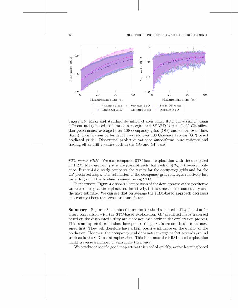
42 CHAPTER 4. PREDICTING AND EXPLORING SCENES
0 20 40 600.7
0.8
0.9
Measurement steps /50
Are
au
nd
erR
OC
0 20 40 600.85
0.9
0.95
1
Measurement steps /50
Are
au
nd
erR
OC
Variance Mean Variance STD Trade Off Mean
Trade Off STD Discount Mean Discount STD
Figure 4.6: Mean and standard deviation of area under ROC curve (AUC) usingdifferent utility-based exploration strategies and SEARD kernel. Left) Classifica-tion performance averaged over 100 occupancy grids (OG) and shown over time.Right) Classification performance averaged over 100 Gaussian Process (GP) basedpredicted grids. Discounted predictive variance outperforms pure variance andtrading off as utility values both in the OG and GP case.
STC versus PRM We also compared STC based exploration with the one basedon PRM. Measurement paths are planned such that each ci ∈ Pu is traversed onlyonce. Figure 4.8 directly compares the results for the occupancy grids and for theGP predicted maps. The estimation of the occupancy grid converges relatively fasttowards ground truth when traversed using STC.
Furthermore, Figure 4.8 shows a comparison of the development of the predictivevariance during haptic exploration. Intuitively, this is a measure of uncertainty overthe map estimate. We can see that on average the PRM-based approach decreasesuncertainty about the scene structure faster.
Summary Figure 4.8 contains the results for the discounted utility function fordirect comparison with the STC-based exploration. GP predicted maps traversedbased on the discounted utility are more accurate early in the exploration process.This is an expected result since here points of high variance are chosen to be mea-sured first. They will therefore have a high positive influence on the quality of theprediction. However, the occupancy grid does not converge as fast towards groundtruth as in the STC-based exploration. This is because the PRM-based explorationmight traverse a number of cells more than once.
We conclude that if a good map estimate is needed quickly, active learning based
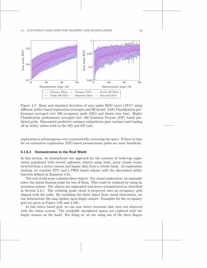
4.1. OCCUPANCY GRID MAPS FOR GRASPING AND MANIPULATION 43
0 20 40 600.7
0.8
0.9
Measurement steps /50
Are
au
nd
erR
OC
0 20 40 600.85
0.9
0.95
1
Measurement steps /50A
rea
un
der
RO
C
Variance Mean Variance STD Trade Off Mean
Trade Off STD Discount Mean Discount STD
Figure 4.7: Mean and standard deviation of area under ROC curve (AUC) usingdifferent utility-based exploration strategies and SE kernel. Left) Classification per-formance averaged over 100 occupancy grids (OG) and shown over time. Right)Classification performance averaged over 100 Gaussian Process (GP) based pre-dicted grids. Discounted predictive variance outperforms pure variance and tradingoff as utility values both in the OG and GP case.
exploration is advantageous over systematically traversing the space. If there is timefor an exhaustive exploration, STC-based measurement paths are more beneficial.
4.1.6.2 Demonstration in the Real World
In this section, we demonstrate our approach for the scenario of table-top explo-ration populated with several unknown objects using both, point clouds recon-structed from a stereo camera and haptic data from a robotic hand. As explorationstrategy we consider STC and a PRM based scheme with the discounted utilityfunction defined in Equation 4.25.
The real world scene contains three objects. For visual exploration, we manuallyselect the initial fixation point for two of them. This could be replaced by using anattention system. The objects are segmented and stereo reconstructed as describedin Section 2.2.1. The resulting point cloud is projected onto an occupancy gridaligned with the table. By excluding the third object from visual observation, wecan demonstrate the map update upon finger contact. Examples for the occupancygrid are given in Figure 4.9b and 4.10b.
In this stereo based grid, we can now detect locations that were not observedwith the vision system. The reachable unexplored spaces are explored with thehaptic sensors on the hand. For doing so, we are using one of the three fingers
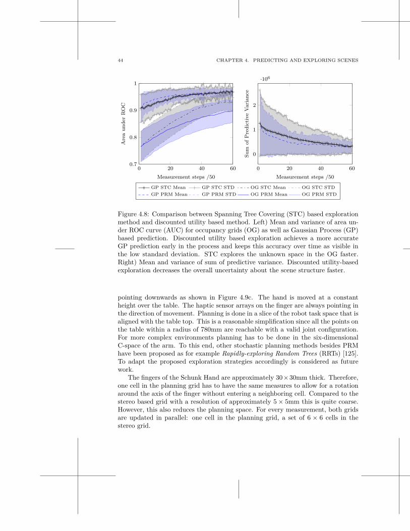
44 CHAPTER 4. PREDICTING AND EXPLORING SCENES
0 20 40 600.7
0.8
0.9
1
Measurement steps /50
Are
au
nd
erR
OC
0 20 40 60
0
1
2
·106
Measurement steps /50
Su
mof
Pre
dic
tive
Vari
an
ce
GP STC Mean GP STC STD OG STC Mean OG STC STD
GP PRM Mean GP PRM STD OG PRM Mean OG PRM STD
Figure 4.8: Comparison between Spanning Tree Covering (STC) based explorationmethod and discounted utility based method. Left) Mean and variance of area un-der ROC curve (AUC) for occupancy grids (OG) as well as Gaussian Process (GP)based prediction. Discounted utility based exploration achieves a more accurateGP prediction early in the process and keeps this accuracy over time as visible inthe low standard deviation. STC explores the unknown space in the OG faster.Right) Mean and variance of sum of predictive variance. Discounted utility-basedexploration decreases the overall uncertainty about the scene structure faster.
pointing downwards as shown in Figure 4.9c. The hand is moved at a constantheight over the table. The haptic sensor arrays on the finger are always pointing inthe direction of movement. Planning is done in a slice of the robot task space that isaligned with the table top. This is a reasonable simplification since all the points onthe table within a radius of 780mm are reachable with a valid joint configuration.For more complex environments planning has to be done in the six-dimensionalC-space of the arm. To this end, other stochastic planning methods besides PRMhave been proposed as for example Rapidly-exploring Random Trees (RRTs) [125].To adapt the proposed exploration strategies accordingly is considered as futurework.
The fingers of the Schunk Hand are approximately 30×30mm thick. Therefore,one cell in the planning grid has to have the same measures to allow for a rotationaround the axis of the finger without entering a neighboring cell. Compared to thestereo based grid with a resolution of approximately 5 × 5mm this is quite coarse.However, this also reduces the planning space. For every measurement, both gridsare updated in parallel: one cell in the planning grid, a set of 6 × 6 cells in thestereo grid.
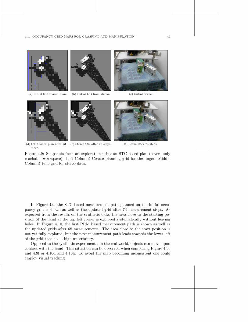
4.1. OCCUPANCY GRID MAPS FOR GRASPING AND MANIPULATION 45
(a) Initial STC based plan. (b) Initial OG from stereo. (c) Initial Scene.
(d) STC based plan after 73steps.
(e) Stereo OG after 73 steps. (f) Scene after 73 steps.
Figure 4.9: Snapshots from an exploration using an STC based plan (covers onlyreachable workspace). Left Column) Coarse planning grid for the finger. MiddleColumn) Fine grid for stereo data.
In Figure 4.9, the STC based measurement path planned on the initial occu-pancy grid is shown as well as the updated grid after 73 measurement steps. Asexpected from the results on the synthetic data, the area close to the starting po-sition of the hand at the top left corner is explored systematically without leavingholes. In Figure 4.10, the first PRM based measurement path is shown as well asthe updated grids after 68 measurements. The area close to the start position isnot yet fully explored, but the next measurement path leads towards the lower leftof the grid that has a high uncertainty.
Opposed to the synthetic experiments, in the real world, objects can move uponcontact with the hand. This situation can be observed when comparing Figure 4.9cand 4.9f or 4.10d and 4.10h. To avoid the map becoming inconsistent one couldemploy visual tracking.
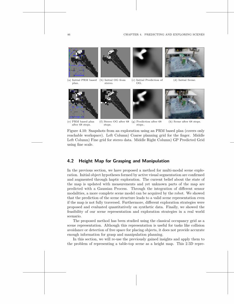
46 CHAPTER 4. PREDICTING AND EXPLORING SCENES
(a) Initial PRM basedplan.
(b) Initial OG fromstereo.
(c) Initial Prediction ofOG.
(d) Initial Scene.
(e) PRM based planafter 68 steps.
(f) Stereo OG after 68steps.
(g) Prediction after 68steps..
(h) Scene after 68 steps.
Figure 4.10: Snapshots from an exploration using an PRM based plan (covers onlyreachable workspace). Left Column) Coarse planning grid for the finger. MiddleLeft Column) Fine grid for stereo data. Middle Right Column) GP Predicted Gridusing fine scale.
4.2 Height Map for Grasping and Manipulation
In the previous section, we have proposed a method for multi-modal scene explo-ration. Initial object hypotheses formed by active visual segmentation are confirmedand augmented through haptic exploration. The current belief about the state ofthe map is updated with measurements and yet unknown parts of the map arepredicted with a Gaussian Process. Through the integration of different sensormodalities, a more complete scene model can be acquired by the robot. We showedthat the prediction of the scene structure leads to a valid scene representation evenif the map is not fully traversed. Furthermore, different exploration strategies wereproposed and evaluated quantitatively on synthetic data. Finally, we showed thefeasibility of our scene representation and exploration strategies in a real worldscenario.
The proposed method has been studied using the classical occupancy grid as ascene representation. Although this representation is useful for tasks like collisionavoidance or detection of free space for placing objects, it does not provide accurateenough information for grasp and manipulation planning.
In this section, we will re-use the previously gained insights and apply them tothe problem of representing a table-top scene as a height map. This 2.5D repre-
4.2. HEIGHT MAP FOR GRASPING AND MANIPULATION 47
sentation is good compromise between a traditional occupancy grid and a full 3Dreconstruction. It provides a simplified 3D model and is therefore better suitedfor manipulation and grasp planning. In [85], the authors showed that a 2.5Drepresentation provides a good surface model and is more efficient than a full 3Dreconstruction at the expense of some details.
As opposed to the previous approach in which scene understanding was posedas a classification problem (free or occupied space), here we treat it as a regressionproblem. As an exploration strategy, we adopt the PRM method using a discountedutility function that we showed to work best for rapidly producing a valid sceneprediction. As a covariance function, we use the simple squared exponential kernelthat provides the most suitable prior in our scenario.
Additionally, we will study the performance of different inference methods.While in the previous section we have used a sampling approach, here we willalso evaluate approximate inference methods.
As an additional virtual sensing modality, we will consider object recognitionand pose estimation.
4.2.1 Scene Representation
The height map, which is aligned with the table top, uniformly subdivides the sceneinto N cells ci with coordinates (wi, vi). Each cell has a state xi that specifies itsheight hi. We model xi as a normally distributed random variable with mean xi
and covariance Pi. Our goal is to obtain an estimate xi for the real state xi givena sensor measurement zt at the point t in time. We use the Kalman Filter as anestimator. Since we are assuming a static environment, the process model thatpredicts how the state of a cell changes over time becomes trivial:
xi,t+1 = xi,t (4.26)
where t and t + 1 indicate subsequent points in time. We are considering threedifferent sensor modalities sr, all providing a height measurement directly. Weassume that the measurement noise ǫr ∼ N (0, Rr) of each of them is additive andGaussian with zero mean and a specific covariance Rr. The details of these modelsare explained in further detail in Section 4.2.2. The measurement model that relatesthe true state xi of a cell ci to a noisy measurement z(i,r) is therefore
z(i,r) = xi + ǫr. (4.27)
We define X = {ci | 0 < i < N}, as the complete map estimate. Let X = Xk ∪ Xu
where Xk is the set of cells whose height value has already been estimated basedon observations. Xu is the set of cells that has not been observed yet.
Additionally to updating the state estimate xi for each cell ci with each observa-tion, we also update the covariance Pi. Intuitively, we can see Pi as a representationof the uncertainty about xi. The smaller it is, the more reliable is the current stateestimate. Equivalent to X , we define P = {Pi | 0 < i < N} as the completeuncertainty map consisting of P = Pk ∪ Pu.
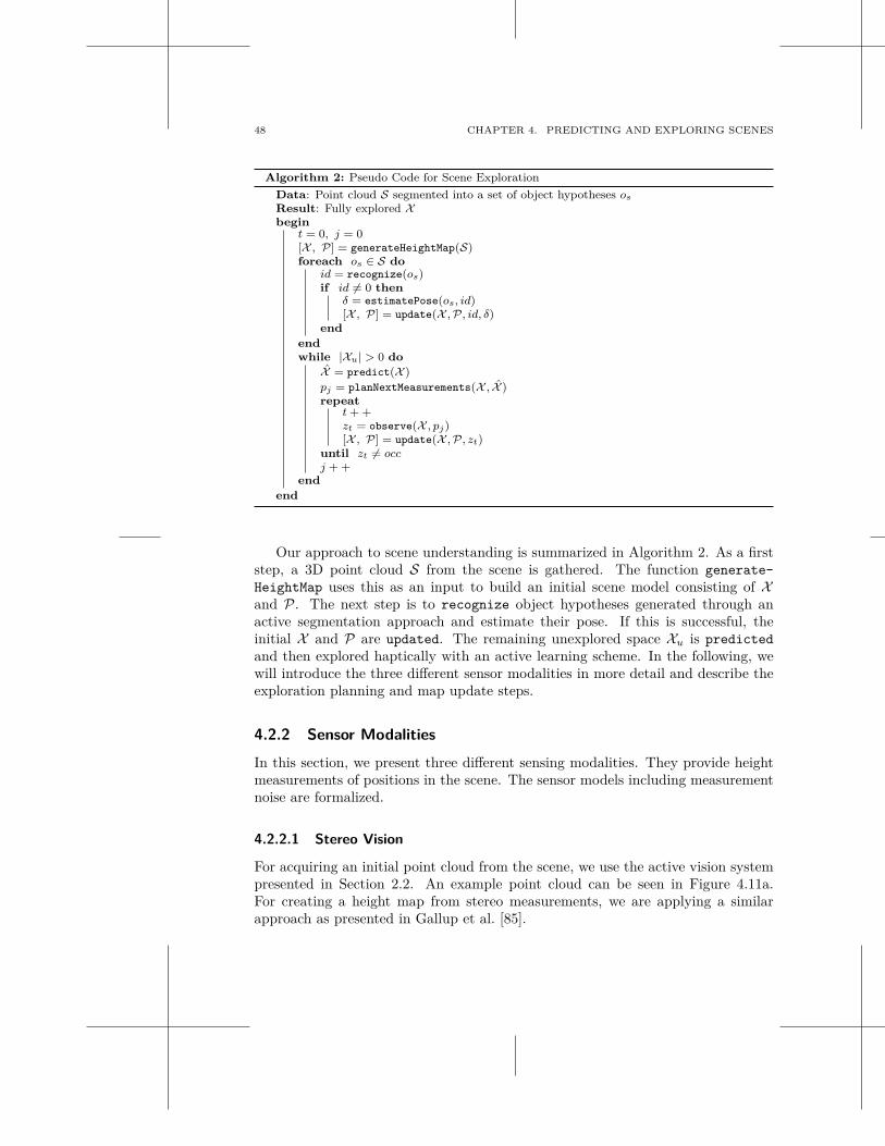
48 CHAPTER 4. PREDICTING AND EXPLORING SCENES
Algorithm 2: Pseudo Code for Scene Exploration
Data: Point cloud S segmented into a set of object hypotheses os
Result: Fully explored Xbegin
t = 0, j = 0[X , P] = generateHeightMap(S)foreach os ∈ S do
id = recognize(os)if id 6= 0 then
δ = estimatePose(os, id)[X , P] = update(X , P, id, δ)
end
end
while |Xu| > 0 do
X = predict(X )
pj = planNextMeasurements(X , X )repeat
t + +zt = observe(X , pj)[X , P] = update(X , P, zt)
until zt 6= occj + +
end
end
Our approach to scene understanding is summarized in Algorithm 2. As a firststep, a 3D point cloud S from the scene is gathered. The function generate-
HeightMap uses this as an input to build an initial scene model consisting of Xand P. The next step is to recognize object hypotheses generated through anactive segmentation approach and estimate their pose. If this is successful, theinitial X and P are updated. The remaining unexplored space Xu is predicted
and then explored haptically with an active learning scheme. In the following, wewill introduce the three different sensor modalities in more detail and describe theexploration planning and map update steps.
4.2.2 Sensor Modalities
In this section, we present three different sensing modalities. They provide heightmeasurements of positions in the scene. The sensor models including measurementnoise are formalized.
4.2.2.1 Stereo Vision
For acquiring an initial point cloud from the scene, we use the active vision systempresented in Section 2.2. An example point cloud can be seen in Figure 4.11a.For creating a height map from stereo measurements, we are applying a similarapproach as presented in Gallup et al. [85].
4.2. HEIGHT MAP FOR GRASPING AND MANIPULATION 49
From Point Cloud to Height Map The basis of the height map computationis formed by a probabilistic 3D occupancy grid of the point cloud. We use thetechnique proposed in Wurm et al. [233] that computes an octree for an efficientdecomposition of the space. The method employs the occupancy update techniqueproposed by Moravec and Elfes [157]. Given a uniform prior (p(v) = 0.5) over thewhole grid, all the stereo observations are incorporated to determine the probabilityof each voxel v to be occupied.
In detail, the value of the vote φv for each voxel is computed as follows:
φv =
{
−1 if l(v) < lfree,
+1 if l(v) > locc.
where l(v) returns the current log occupancy value of voxel v. As threshold, we uselog occupancy values of locc = 0.85 and lfree = -0.4, corresponding to probabilitiesof 0.7 and 0.4 for free and occupied volumes as proposed by Wurm et al. [233].
Given these votes, our goal is to compute the height of all cells ci on the table.Let {vj}Ni
refer to the set of voxels that have the same (w, v) coordinates as ci
but whose voxel center is positioned at different heights hj . They can also be seenas a column on cell ci. Then the height value h(i,1) of this cell is chosen to be
c∗(i,1) = min
hj
∑
v∈V>hj
φv −∑
v∈V<hj
φv (4.28)
h(i,1) = arghjc∗
(i,1). (4.29)
The set V>hjcontains all those voxels whose height is bigger than hj . Similarly,
V<hjcontains all those voxels whose height is smaller than hj . This minimisation
results in a height estimate h(i,1) in which the majority of voxels below it areoccupied and the majority of voxel above it are empty. An example for the estimatedheight map of the point cloud in Figure 4.11a is shown in Figure 4.11b and 4.11c.An example for a cost map containing c∗
(i,1) as computed in Equation 4.28 is shownin Figure 4.11d. Given Ni voxels with φv 6= 0 in the column on cell ci, c∗
(i,1) canhave values between −Ni and 0. We therefore normalise and shift this cost to mapit to a range between 0 and 1.
c(i,1) =c∗
(i,1)
Ni+ 1 (4.30)
Measurement Noise Model As discussed above, each measurement modalityr has an individual noise model with ǫr ∼ N (0, Rr). The measurement covarianceR1 for stereo vision and a specific cell ci is computed as follows. The normalizedcost value c(i,1) of choosing h(i,1) will be high for columns that contain many noisy3D points. For the corresponding cells on the table, we want this uncertainty about
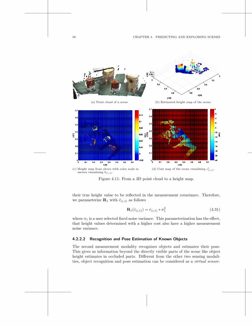
50 CHAPTER 4. PREDICTING AND EXPLORING SCENES
(a) Point cloud of a scene (b) Estimated height map of the scene.
(c) Height map from above with color scale inmeters visualizing h(i,1).
(d) Cost map of the scene visualizing c∗
(i,1).
Figure 4.11: From a 3D point cloud to a height map.
their true height value to be reflected in the measurement covariance. Therefore,we parameterize R1 with c(i,1) as follows
R1(c(i,1)) = c(i,1) ∗ σ21 (4.31)
where σ1 is a user selected fixed noise variance. This parameterization has the effect,that height values determined with a higher cost also have a higher measurementnoise variance.
4.2.2.2 Recognition and Pose Estimation of Known Objects
The second measurement modality recognizes objects and estimates their pose.This gives us information beyond the directly visible parts of the scene like objectheight estimates in occluded parts. Different from the other two sensing modali-ties, object recognition and pose estimation can be considered as a virtual sensor .
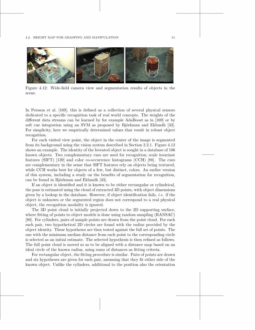
4.2. HEIGHT MAP FOR GRASPING AND MANIPULATION 51
Figure 4.12: Wide-field camera view and segmentation results of objects in thescene.
In Persson et al. [169], this is defined as a collection of several physical sensorsdedicated to a specific recognition task of real world concepts. The weights of thedifferent data streams can be learned by for example AdaBoost as in [169] or bysoft cue integration using an SVM as proposed by Björkman and Eklundh [33].For simplicity, here we empirically determined values that result in robust objectrecognition.
For each visited view point, the object in the center of the image is segmentedfrom its background using the vision system described in Section 2.2.1. Figure 4.12shows an example. The identity of the foveated object is sought in a database of 106known objects. Two complementary cues are used for recognition; scale invariantfeatures (SIFT) [139] and color co-occurrence histograms (CCH) [88]. The cuesare complementary in the sense that SIFT features rely on objects being textured,while CCH works best for objects of a few, but distinct, colors. An earlier versionof this system, including a study on the benefits of segmentation for recognition,can be found in Björkman and Eklundh [33].
If an object is identified and it is known to be either rectangular or cylindrical,the pose is estimated using the cloud of extracted 3D points, with object dimensionsgiven by a lookup in the database. However, if object identification fails, i.e. if theobject is unknown or the segmented region does not correspond to a real physicalobject, the recognition modality is ignored.
The 3D point cloud is initially projected down to the 2D supporting surface,where fitting of points to object models is done using random sampling (RANSAC)[80]. For cylinders, pairs of sample points are drawn from the point cloud. For eachsuch pair, two hypothetical 2D circles are found with the radius provided by theobject identity. These hypotheses are then tested against the full set of points. Theone with the minimum median distance from each point to the corresponding circleis selected as an initial estimate. The selected hypothesis is then refined as follows.The full point cloud is moved so as to be aligned with a distance map based on anideal circle of the known radius, using sums of distances as fitting criteria.
For rectangular object, the fitting procedure is similar. Pairs of points are drawnand six hypotheses are given for each pair, assuming that they fit either side of theknown object. Unlike the cylinders, additional to the position also the orientation
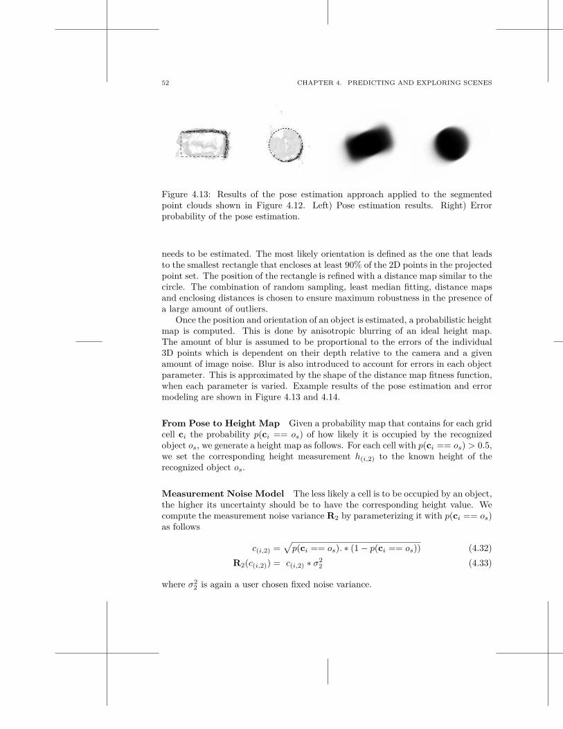
52 CHAPTER 4. PREDICTING AND EXPLORING SCENES
Figure 4.13: Results of the pose estimation approach applied to the segmentedpoint clouds shown in Figure 4.12. Left) Pose estimation results. Right) Errorprobability of the pose estimation.
needs to be estimated. The most likely orientation is defined as the one that leadsto the smallest rectangle that encloses at least 90% of the 2D points in the projectedpoint set. The position of the rectangle is refined with a distance map similar to thecircle. The combination of random sampling, least median fitting, distance mapsand enclosing distances is chosen to ensure maximum robustness in the presence ofa large amount of outliers.
Once the position and orientation of an object is estimated, a probabilistic heightmap is computed. This is done by anisotropic blurring of an ideal height map.The amount of blur is assumed to be proportional to the errors of the individual3D points which is dependent on their depth relative to the camera and a givenamount of image noise. Blur is also introduced to account for errors in each objectparameter. This is approximated by the shape of the distance map fitness function,when each parameter is varied. Example results of the pose estimation and errormodeling are shown in Figure 4.13 and 4.14.
From Pose to Height Map Given a probability map that contains for each gridcell ci the probability p(ci == os) of how likely it is occupied by the recognizedobject os, we generate a height map as follows. For each cell with p(ci == os) > 0.5,we set the corresponding height measurement h(i,2) to the known height of therecognized object os.
Measurement Noise Model The less likely a cell is to be occupied by an object,the higher its uncertainty should be to have the corresponding height value. Wecompute the measurement noise variance R2 by parameterizing it with p(ci == os)as follows
c(i,2) =√
p(ci == os). ∗ (1 − p(ci == os)) (4.32)
R2(c(i,2)) = c(i,2) ∗ σ22 (4.33)
where σ22 is again a user chosen fixed noise variance.
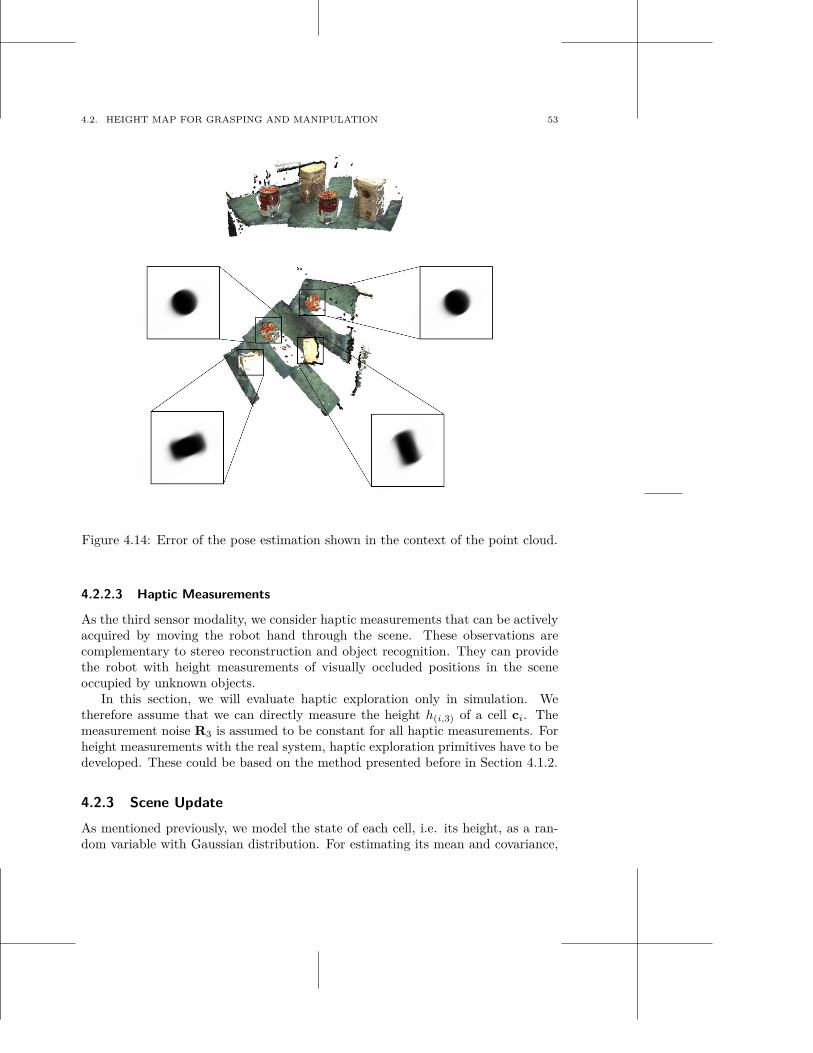
4.2. HEIGHT MAP FOR GRASPING AND MANIPULATION 53
Figure 4.14: Error of the pose estimation shown in the context of the point cloud.
4.2.2.3 Haptic Measurements
As the third sensor modality, we consider haptic measurements that can be activelyacquired by moving the robot hand through the scene. These observations arecomplementary to stereo reconstruction and object recognition. They can providethe robot with height measurements of visually occluded positions in the sceneoccupied by unknown objects.
In this section, we will evaluate haptic exploration only in simulation. Wetherefore assume that we can directly measure the height h(i,3) of a cell ci. Themeasurement noise R3 is assumed to be constant for all haptic measurements. Forheight measurements with the real system, haptic exploration primitives have to bedeveloped. These could be based on the method presented before in Section 4.1.2.
4.2.3 Scene Update
As mentioned previously, we model the state of each cell, i.e. its height, as a ran-dom variable with Gaussian distribution. For estimating its mean and covariance,
54 CHAPTER 4. PREDICTING AND EXPLORING SCENES
we use the Kalman Filter. Following the process and measurement model fromEquation 4.26 and 4.27, we update the state estimate xi and covariance Pi for cellci at time t + 1 as follows:
x−i,t+1 = xi,t
P−i,t+1 = Pi,t
Ki,t+1 =P−
i,t+1
P−i,t+1 + Rr
(4.34)
xi,t+1 = x−i,t+1 + Ki,t+1(z(i,t+1,r) − x−
i,t+1)
Pi,t+1 = (I − Ki,t+1)P−i,t+1
given an observation z(i,t+1,r) made with modality r.
4.2.4 Scene Prediction
In traditional exploration techniques, no assumptions are made about places inspace that have not been observed yet. In accordance with related work [162, 85],we have shown in Section 4.1 that we can make use of spatial correlation to predictthe structure of an environment based on already measured parts of it.
Spatial correlation in our case means, we know that cells in the grid that areclose to occupied spaces but are due to occlusions not directly observable, are likelyto be part of the occluding object. By modeling this spatial correlation betweenphysically close locations in the environment, we can predict unobserved placesfrom observed ones. Then instead of exploring the whole environment exhaustivelywe can select to confirm the predicted map at specifically uncertain places. InSection 4.1 we have shown the spatial correlation in a 2D occupancy grid can bemodeled with a Gaussian Process. The assumption of independence of neighboringcells in a traditional occupancy grid is then removed.
In this section, we are using a height map instead of an occupancy grid. We willshow that also in this representation spatial correlation can be similarly modeledwith a GP. Compared to the previous section, scene prediction is conducted throughGaussian Process Regression instead of Classification of cells into occupied or empty.Given a set of input values x and the corresponding target values y, the goal of GPregression is to estimate the latent function g(·) that generated these samples. Inour case, x is constituted by the set of observed cells ck ∈ Pk. The target values y
are the corresponding noisy height estimates hk. Together they form the trainingset {xi, yi}M with cardinality M . As has already been detailed in Section 4.1.4.1,the relation between the input and target values assuming Gaussian additive noisecan be modelled as
g(xi) = φ(xi)T w, yi = g(xi) + ǫ
w is a vector of weight parameters of the linear model. φ(xi) is a function thatmaps D-dimensional input data into an N -dimensional feature space.
4.2. HEIGHT MAP FOR GRASPING AND MANIPULATION 55
From this formulation, we can derive the posterior likelihood of the weightparameters given the training data. Primarily, we are interested in predicting thestate y′ = hj of an unobserved cell cj ∈ Pu referred to as x′ in the following.In Section 4.1.4.1, we have shown that this prediction g(x′) ∼ N (µ, Σ) follows aGaussian distribution with
µ = k(x′, x)T [K(x, x) + σ2M I]−1y
Σ = k(x′, x′) − k(x′, x)T [K(x, x) + σ2M I]−1k(x′, x).
The Gram matrix K(x, x) is computed based on a covariance function k(·, ·). InSection 4.1, we showed that the squared exponential covariance function is a goodprior for our scenario. Therefore, we are using it for the height map representationas well. An example for this prediction given a 2D map of a partially explored sceneis given in Figure. In Section 4.2.6, we will show quantitatively on synthetic datathat a GP predicted map is a reasonable estimate of the ground truth.
Inference Methods To predict the height value of an unobserved cell x′ and itsuncertainty, we need to evaluate the mean and variance of g(x′). Especially, thecomputation of the variance is expensive since it involves inverting the covariancematrix K(x, x). If the set Pk of previously observed grid cells is of cardinality M ,then K is of dimension M × M . Hence, inverting K is of complexity O(M3).
Ideally, we would like the robot to be able to represent, predict and explorea scene of its current radius of action in real-time. Therefore, we not only needan efficient scene representation that scales well to different resolutions, but alsoan efficient inference method for prediction. In this section, we will evaluate andcompare three different inference methods.
Confidence-based Sampling In Section 4.1, we used a sampling approach in whichdata points are sampled according to their confidence. In this section, we will usethe uncertainty map Pk containing the covariance values Pi of all observed grid cellsci in Xk. Cells with a smaller covariance, i.e., a smaller uncertainty about theirheight estimate, are more likely to be part of the training set x. This set will containa fixed number of samples from free and from occupied space. The number of freesamples will be higher than the number of occupied samples, thereby reflectingstructure of the scene.
Uniform Sampling Additionally to the confidence-based sampling, we will alsouse uniform sampling to assemble the training set x. The same number of free andoccupied samples are drawn as for the confidence-based case.
Subset of Regressors The aforementioned sampling methods only consider the se-lected subset of the observed grid cells for constructing the Gram matrix K. A dif-ferent approximation to the full GP regression problem is proposed in [181] which
56 CHAPTER 4. PREDICTING AND EXPLORING SCENES
we will briefly summarize here. It also relies on a subset of regressors (SR). How-ever, it takes the correlation of this subset to the remaining data in the training setinto account.
It has been shown that the mean predictor of g(x′) can be obtained by formu-lating it as a finite-dimensional generalized linear regression model:
g(x′) =M
∑
i=1
αik(x′, xi) with α ∼ N (0, K−1). (4.35)
If we consider only a subset {xj , yj}N of regressors of cardinality N , then Equa-tion 4.35 becomes
gSR(x′) =N
∑
j=1
αjk(x′, xj) with αj ∼ N (0, K−1jj ). (4.36)
Given the subset of regressor as xSR, it follows that gSR(x′) ∼ N (µSR, ΣSR) with
µSR = k(x′, xSR)T [KNM KMN + σ2M KNN ]−1y (4.37)
ΣSR = σ2M k(x′, xSR)T [KNM KMN + σ2
M KNN ]−1k(x′, xSR). (4.38)
To keep the notation uncluttered, KNM refers to K(xSR, x), KMN to K(x, xSR)and equivalently KNN to K(xSR, xSR). The matrix computations in Equation 4.37and 4.38 are then of complexity O(N2M). Evaluating the mean takes time O(M)and the variance O(M2).
Note that under the SR model, the covariance function of two data points xi andxj becomes k(xi, xj) = k(xi, xSR)T K−1
NN k(xj , xSR) and is therefore only dependenton the correlation with the so called active set. This leaves the question, how thisset is chosen. Many different methods have been proposed in the literature. Here,we will use the result from the confidence-based sampling as the subset of regressors.
4.2.5 Active Exploration
Given a partial map of the environment, we want to efficiently explore the remain-ing unknown parts with haptic sensors. Efficiently here means that we want tominimize the number of measurement actions needed to reach a sufficient under-standing about the scene as quickly as possible. In Section 4.1, we found thatan active learning scheme based on PRM path planning in combination with adiscounted utility function performs best when the goal is to reach a valid sceneprediction already early on in the exploration process. This scheme supports theGaussian Process based map prediction by selecting most informative observations,i.e., measurements that maximise the expected gain in Shannon information.
4.2.6 Experiments
We evaluate the proposed approach quantitatively on synthetic data. We are specif-ically interested in analyzing how well a Gaussian Process can predict a height map
4.2. HEIGHT MAP FOR GRASPING AND MANIPULATION 57
from partial observations compared to different baselines. In that context, we willalso study the three inference methods we proposed.
Furthermore, we will explore how much the different sensor modalities improvethe prediction. Additionally to stereo vision, we consider object recognition incombination with pose estimation and haptic exploration.
4.2.6.1 Data Set
We generated 50 different synthetic environments (1000 × 1000 mm) of the kindshown in Figure 4.15g. Every scene contains ten objects that can either be ofcylindrical or box shape and are spread on a table. Their intrinsic attributes likeheight, aspect ratio or radius as well as their extrinsic attributes like position andorientation were chosen randomly within pre-determined ranges. Overlapping ofobjects was allowed so that fewer than ten connected components can occur as wellas more complex shapes.
For every scene, we simulated three camera observations such that in each ofthem one randomly chosen object is in fixation. This is close to our real active vi-sion system in which stereo reconstruction is performed once an object is properlyfixated. For each observation, we reconstruct a point cloud using the ray-tracer Ya-faRay [234]. We model the noise from the stereo system by assuming zero-meanGaussian noise of a specific covariance in the image. This results in a point cloudwith stronger noise in locations that are farer away from the camera. An examplefor the camera observation as well as the point clouds can be seen in Figures 4.15ato 4.15f. The height maps corresponding to the observations were computed asdescribed in Section 4.2.2.1. For obtaining an initial height map estimate X aswell as a corresponding uncertainty map P, the update Equations 4.34 with thecorresponding noise covariance in Equation 4.31 are applied.
We assumed that each of the three fixated objects got segmented and recognizedso that their pose can be estimated from the segmented point cloud as described inSection 4.2.2.2. Examples for the recognition results on the synthetic data can beseen in Figure 4.15h to 4.15m. This results in three additional height and cost mapsthat can be used to update the current X and P. The same update equations as forthe height maps from stereo measurements are applied with the noise covariancecorresponding to the recognition sensor modality.
The difference between the state estimate and corresponding covariance withand without the recognition results can be observed in Figure 4.16. The heightmap that includes additional recognition results is more complete. The covarianceof this map shows more certainty about height estimates at the center of recognizedobjects and more uncertainty at their boundaries.
4.2.6.2 Measure of Comparison
We considered the problem of height map estimation as a regression problem. Asa measure of divergence between ground truth and the estimated scene, we use the
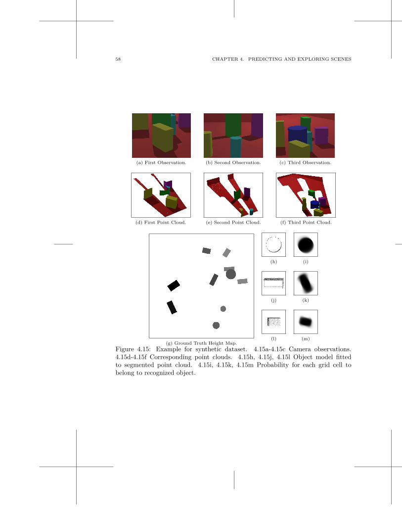
58 CHAPTER 4. PREDICTING AND EXPLORING SCENES
(a) First Observation. (b) Second Observation. (c) Third Observation.
(d) First Point Cloud. (e) Second Point Cloud. (f) Third Point Cloud.
(g) Ground Truth Height Map.
(h) (i)
(j) (k)
(l) (m)
Figure 4.15: Example for synthetic dataset. 4.15a-4.15c Camera observations.4.15d-4.15f Corresponding point clouds. 4.15h, 4.15j, 4.15l Object model fittedto segmented point cloud. 4.15i, 4.15k, 4.15m Probability for each grid cell tobelong to recognized object.
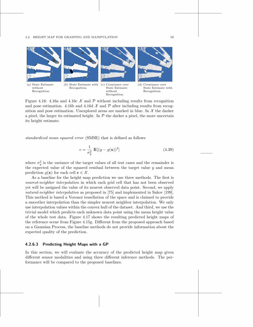
4.2. HEIGHT MAP FOR GRASPING AND MANIPULATION 59
(a) State EstimatewithoutRecognition.
(b) State Estimate withRecognition.
(c) Covariance overState EstimatewithoutRecognition.
(d) Covariance overState Estimate withRecognition.
Figure 4.16: 4.16a and 4.16c X and P without including results from recognitionand pose estimation. 4.16b and 4.16d X and P after including results from recog-nition and pose estimation. Unexplored areas are marked in blue. In X the darkera pixel, the larger its estimated height. In P the darker a pixel, the more uncertainits height estimate.
standardized mean squared error (SMSE) that is defined as follows
e =1σ2
y
IE[(y − g(x))2] (4.39)
where σ2y is the variance of the target values of all test cases and the remainder is
the expected value of the squared residual between the target value y and meanprediction g(x) for each cell c ∈ X .
As a baseline for the height map prediction we use three methods. The first isnearest-neighbor interpolation in which each grid cell that has not been observedyet will be assigned the value of its nearest observed data point. Second, we applynatural-neighbor interpolation as proposed in [75] and implemented in Sakov [199].This method is based a Voronoi tessellation of the space and is claimed to providea smoother interpolation than the simpler nearest neighbor interpolation. We onlyuse interpolation values within the convex hull of the dataset. And third, we use thetrivial model which predicts each unknown data point using the mean height valueof the whole test data. Figure 4.17 shows the resulting predicted height maps ofthe reference scene from Figure 4.15g. Different from the proposed approach basedon a Gaussian Process, the baseline methods do not provide information about theexpected quality of the prediction.
4.2.6.3 Predicting Height Maps with a GP
In this section, we will evaluate the accuracy of the predicted height map givendifferent sensor modalities and using three different inference methods. The per-formance will be compared to the proposed baselines.
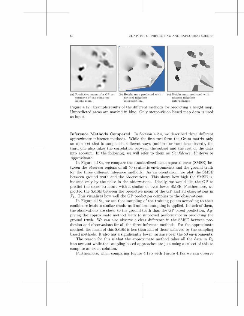
60 CHAPTER 4. PREDICTING AND EXPLORING SCENES
(a) Predictive mean of a GP asestimate of the completeheight map.
(b) Height map predicted withnatural-neighborinterpolation.
(c) Height map predicted withnearest-neighborInterpolation
Figure 4.17: Example results of the different methods for predicting a height map.Unpredicted areas are marked in blue. Only stereo-vision based map data is usedas input.
Inference Methods Compared In Section 4.2.4, we described three differentapproximate inference methods. While the first two form the Gram matrix onlyon a subset that is sampled in different ways (uniform or confidence-based), thethird one also takes the correlation between the subset and the rest of the datainto account. In the following, we will refer to them as Confidence, Uniform orApproximate.
In Figure 4.18a, we compare the standardized mean squared error (SMSE) be-tween the observed regions of all 50 synthetic environments and the ground truthfor the three different inference methods. As an orientation, we plot the SMSEbetween ground truth and the observations. This shows how high the SMSE is,induced only by the noise in the observations. Ideally, we would like the GP topredict the scene structure with a similar or even lower SMSE. Furthermore, weplotted the SMSE between the predictive mean of the GP and all observations inPk. This visualises how well the GP prediction complies to the observations.
In Figure 4.18a, we see that sampling of the training points according to theirconfidence leads to similar results as if uniform sampling is applied. In each of them,the observations are closer to the ground truth than the GP based prediction. Ap-plying the approximate method leads to improved performance in predicting theground truth. We can also observe a clear difference in the SMSE between pre-diction and observations for all the three inference methods. For the approximatemethod, the mean of this SMSE is less than half of those achieved by the samplingbased methods. It also has a significantly lower variance over the 50 environments.
The reason for this is that the approximate method takes all the data in Pk
into account while the sampling based approaches are just using a subset of this tocompute an exact solution.
Furthermore, when comparing Figure 4.18b with Figure 4.18a we can observe
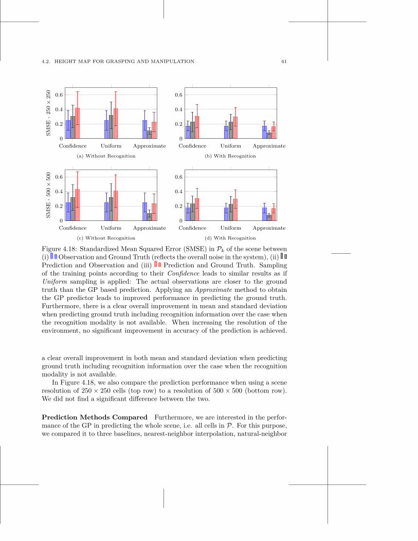
4.2. HEIGHT MAP FOR GRASPING AND MANIPULATION 61
Confidence Uniform Approximate
0
0.2
0.4
0.6
SM
SE
-250
×250
(a) Without Recognition
Confidence Uniform Approximate
0
0.2
0.4
0.6
(b) With Recognition
Confidence Uniform Approximate
0
0.2
0.4
0.6
SM
SE
-500
×500
(c) Without Recognition
Confidence Uniform Approximate
0
0.2
0.4
0.6
(d) With Recognition
Figure 4.18: Standardized Mean Squared Error (SMSE) in Pk of the scene between(i) Observation and Ground Truth (reflects the overall noise in the system), (ii)Prediction and Observation and (iii) Prediction and Ground Truth. Samplingof the training points according to their Confidence leads to similar results as ifUniform sampling is applied: The actual observations are closer to the groundtruth than the GP based prediction. Applying an Approximate method to obtainthe GP predictor leads to improved performance in predicting the ground truth.Furthermore, there is a clear overall improvement in mean and standard deviationwhen predicting ground truth including recognition information over the case whenthe recognition modality is not available. When increasing the resolution of theenvironment, no significant improvement in accuracy of the prediction is achieved.
a clear overall improvement in both mean and standard deviation when predictingground truth including recognition information over the case when the recognitionmodality is not available.
In Figure 4.18, we also compare the prediction performance when using a sceneresolution of 250 × 250 cells (top row) to a resolution of 500 × 500 (bottom row).We did not find a significant difference between the two.
Prediction Methods Compared Furthermore, we are interested in the perfor-mance of the GP in predicting the whole scene, i.e. all cells in P. For this purpose,we compared it to three baselines, nearest-neighbor interpolation, natural-neighbor
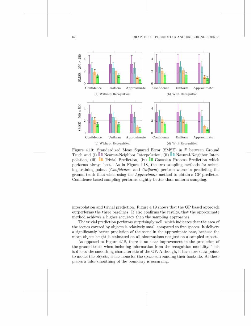
62 CHAPTER 4. PREDICTING AND EXPLORING SCENES
Confidence Uniform Approximate
0
2
4
SM
SE
-250
×250
(a) Without Recognition
Confidence Uniform Approximate
0
2
4
(b) With Recognition
Confidence Uniform Approximate
0
2
4
SM
SE
-500
×500
(c) Without Recognition
Confidence Uniform Approximate
0
2
4
(d) With Recognition
Figure 4.19: Standardized Mean Squared Error (SMSE) in P between GroundTruth and (i) Nearest-Neighbor Interpolation, (ii) Natural-Neighbor Inter-polation, (iii) Trivial Prediction, (iv) Gaussian Process Prediction whichperforms always best. As in Figure 4.18, the two sampling methods for select-ing training points (Confidence and Uniform) perform worse in predicting theground truth than when using the Approximate method to obtain a GP predictor.Confidence based sampling performs slightly better than uniform sampling.
interpolation and trivial prediction. Figure 4.19 shows that the GP based approachoutperforms the three baselines. It also confirms the results, that the approximatemethod achieves a higher accuracy than the sampling approaches.
The trivial prediction performs surprisingly well, which indicates that the area ofthe scenes covered by objects is relatively small compared to free spaces. It deliversa significantly better prediction of the scene in the approximate case, because themean object height is estimated on all observations not just on a sampled subset.
As opposed to Figure 4.18, there is no clear improvement in the prediction ofthe ground truth when including information from the recognition modality. Thisis due to the smoothing characteristic of the GP. Although, it has more data pointsto model the objects, it has none for the space surrounding their backside. At theseplaces a false smoothing of the boundary is occurring.
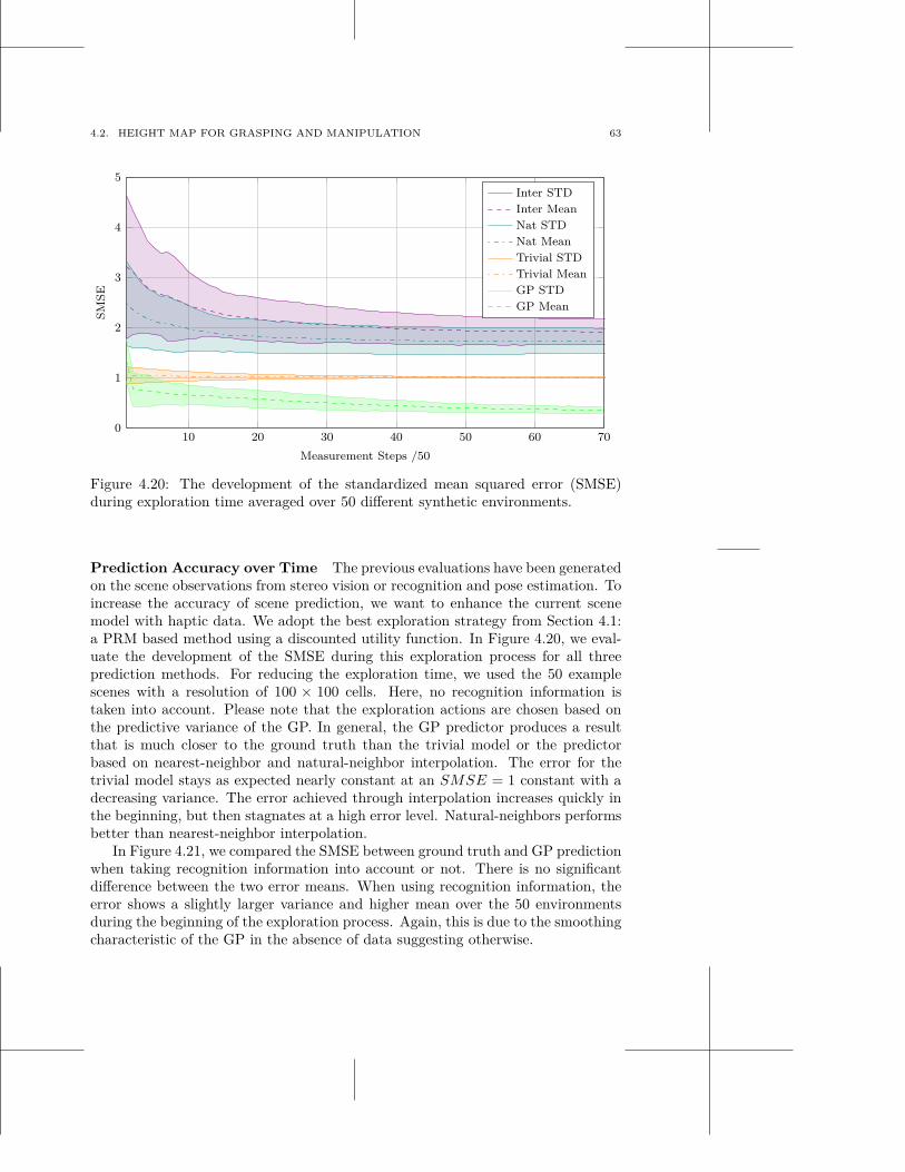
4.2. HEIGHT MAP FOR GRASPING AND MANIPULATION 63
10 20 30 40 50 60 700
1
2
3
4
5
Measurement Steps /50
SM
SE
Inter STD
Inter Mean
Nat STD
Nat Mean
Trivial STD
Trivial Mean
GP STD
GP Mean
Figure 4.20: The development of the standardized mean squared error (SMSE)during exploration time averaged over 50 different synthetic environments.
Prediction Accuracy over Time The previous evaluations have been generatedon the scene observations from stereo vision or recognition and pose estimation. Toincrease the accuracy of scene prediction, we want to enhance the current scenemodel with haptic data. We adopt the best exploration strategy from Section 4.1:a PRM based method using a discounted utility function. In Figure 4.20, we eval-uate the development of the SMSE during this exploration process for all threeprediction methods. For reducing the exploration time, we used the 50 examplescenes with a resolution of 100 × 100 cells. Here, no recognition information istaken into account. Please note that the exploration actions are chosen based onthe predictive variance of the GP. In general, the GP predictor produces a resultthat is much closer to the ground truth than the trivial model or the predictorbased on nearest-neighbor and natural-neighbor interpolation. The error for thetrivial model stays as expected nearly constant at an SMSE = 1 constant with adecreasing variance. The error achieved through interpolation increases quickly inthe beginning, but then stagnates at a high error level. Natural-neighbors performsbetter than nearest-neighbor interpolation.
In Figure 4.21, we compared the SMSE between ground truth and GP predictionwhen taking recognition information into account or not. There is no significantdifference between the two error means. When using recognition information, theerror shows a slightly larger variance and higher mean over the 50 environmentsduring the beginning of the exploration process. Again, this is due to the smoothingcharacteristic of the GP in the absence of data suggesting otherwise.
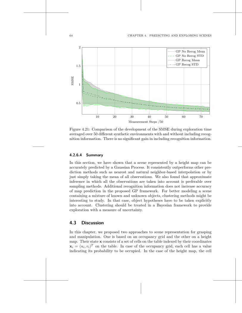
64 CHAPTER 4. PREDICTING AND EXPLORING SCENES
10 20 30 40 50 60 70
0.5
1
1.5
2
Measurement Steps /50
SM
SE
GP No Recog Mean
GP No Recog STD
GP Recog Mean
GP Recog STD
Figure 4.21: Comparison of the development of the SMSE during exploration timeaveraged over 50 different synthetic environments with and without including recog-nition information. There is no significant gain in including recognition information.
4.2.6.4 Summary
In this section, we have shown that a scene represented by a height map can beaccurately predicted by a Gaussian Process. It consistently outperforms other pre-diction methods such as nearest and natural neighbor-based interpolation or byjust simply taking the mean of all observations. We also found that approximateinference in which all the observations are taken into account is preferable oversampling methods. Additional recognition information does not increase accuracyof map prediction in the proposed GP framework. For better modeling a scenecontaining a mixture of known and unknown objects, clustering methods might beinteresting to study. In that case, object hypotheses have to be taken explicitlyinto account. Clustering should be treated in a Bayesian framework to provideexploration with a measure of uncertainty.
4.3 Discussion
In this chapter, we proposed two approaches to scene representation for graspingand manipulation. One is based on an occupancy grid and the other on a heightmap. Their state x consists of a set of cells on the table indexed by their coordinatesxi = (ui, vi)T on the table. In case of the occupancy grid, each cell has a valueindicating its probability to be occupied. In the case of the height map, the cell
4.3. DISCUSSION 65
value corresponds to the height of the object that is occupying this cell. We havealso demonstrated how multiple modalities such as stereo vision, object recognitionand pose estimation as well as haptic sensor data can be integrated into either ofthese representations. Each representation has different utilities in a grasping andmanipulation scenario. The occupancy grid map outlines free and occupied spacesand is therefore suitable for deciding for example on where to place objects that therobot has picked up. A height map on the other hand carries additional informationabout the object height and therefore facilitates grasp planning.
We have shown that a Gaussian Process can be used as an implementation ofthe function g(·) for accurately predicting the value of unobserved cells in the scene.
The remaining challenge is to make this approach capable of real-time pro-cessing. The map of the scene should be predicted and updated rapidly duringinteraction. In this chapter, we have proposed to use knowledge about the tableplane in the scene to reduce the dimensionality of the representation from 3D to2D. Furthermore, we experimented with approximate inference methods. However,these approximate techniques still do not scale well enough to allow for real-timecomputation in large environments. Furthermore, a table plane may not be de-tectable in every scene.
An approach inspired by the ideas by Brooks [46, 47] and from the field ofActive Vision [22, 20] would be to restrict the proposed high-resolution predictionto the task-relevant parts of the scene. Through this limitation, the map could becomputed more often. Changes in the currently interesting part of the scene couldbe taken into account more rapidly.
To illustrate this idea, consider the following scenario. The goal is to pick upan object from a table-top scene. The active head fixates on this object and stereoreconstructs this part of the scene. The object is segmented from the background.However, the scene is only partially known due to occlusions.
Using the proposed approach of height map prediction through a Gaussian Pro-cess, we can predict the whole scene in the current view This information can thenbe used to plan a safe grasp. In this case this means, that the grasp is chosensuch that the probability of the hand colliding with any other object on the tableis minimal.
Furthermore, during the grasp, the environment might change due to movingobjects. By having restricted the map to the region in the current viewpoint, a real-time update of the map that takes these changes into account becomes possible.This would then allow for online adaptation of the grasp parameters.
Once the object is picked up, we might want to put it down at another free spotin the environment. Given an approximate position in space, where this objectshould be put down, the head can start exploring the environment from there untila suitable place is found. Instead of using a fixed size of the scene as in this chapter,it could start from an initial size and extend it on demand.
This application of the scene prediction is in the spirit of active vision andbehavioral robotics in that perception is done rapidly and only on demand in thecontext of certain behavior.
5
Enhanced Scene Understanding throughHuman-Robot Dialog
A full segmentation of all objects in a scene is desirable for many tasks such asrecognition [32], grasp planning [8] or learning models for previously unseen objectsthat are re-usable for later re-recognition. This is a different subproblem of sceneunderstanding from what has been proposed in Chapter 4. In the previous chapter,geometric scene structure was predicted independent of correct object segmentation.
A common problem of vision systems employed for object segmentation is thatthey might incorrectly group objects together or split them into several parts. Thisis commonly referred to as under- or over-segmentation. The two vision systemspresented in Section 2.2 suffer from this limitation as well. The sensitivity to thisproblem depends on how close objects are to each other, how similar they are inappearance and on whether the correct number of objects in the scene is known inadvance.
Interactive segmentation methods that aim at refining the robot’s current scenemodel have recently gained a lot of attention. One approach addressing this prob-lem, is to let the robot interact with the scene, e.g., through pushing movements andthen use motion cues for verifying or refining object hypotheses [114, 151, 110, 28].These papers focus on the question of what knowledge can be gained from observingthe outcomes of robotic actions. The majority of them leaves the question open ofhow to select the action that provides the greatest amount of information.
In this chapter, we propose to put a “human in the loop” to achieve the objectiveof correct scene segmentation. This has the advantage of the robot being capableof learning new labels or symbols online and ground them in the current sensorydata. We move towards this goal by combining state-of-the-art computer visionwith a natural dialog system allowing a human to rapidly refine the model of acomplex 3D scene. Through that approach, we harness the strengths of ‘bottomup’ automated processing with the ‘top down’ decision making power of a humanoperator. The resulting refined scene model forms the basis for a general symbolgrounding problem [96].
Human input is not a new concept in object segmentation and scene under-standing. Several previous systems have used it to guide automated processingor restrict the search space of algorithms both improving efficiency and decreas-
67
68 CHAPTER 5. ENHANCED SCENE UNDERSTANDING THROUGH HUMAN-ROBOT DIALOG
ing false positives [109, 227, 115]. GrabCut [188] and Lazy Snapping [136] are themost related works on interactive segmentation. They require the user to operate amouse either for selecting a region containing the object in the image or for draw-ing its rough outline. In this chapter, we aim for human-robot interaction usingonly natural dialog and no additional tools. Thereby, we are moving closer to howhumans naturally interact with one another in such situations.
Several unique challenges exist when designing a framework for human robotinteraction using computer vision. One of them is to minimize the iteration time ofthe vision component of such a system. This processing must be rapid enough as tonot induce a large lag in the system increasing the mental load on the user [212]. Asmost state-of-the-art vision algorithm for scene understanding run in tens of minutesor hours per scene [215, 143, 134], they would be unacceptable for any “human-in-the-loop” system. Here, we propose to use the multi-object segmentation algorithmpresented in Section 2.2.2, which is capable of providing acceptable responsivenessin the proposed algorithm.
Another design challenge is to minimize the necessary interaction between theautonomous system and the human operator. This means maximizing the valueof each interaction to obtain the greatest discriminatory information. A very com-mon approach to this kind of problem is to make a decision that maximises theexpected gain in information or, equivalently, minimises the uncertainty in the sys-tem [109][3]. In this chapter, we propose the concept of entropy to characterize thequality of any object hypothesis. This helps in guiding the dialog system to resolvethe most challenging and ambiguous segments first.
5.1 System Overview
In the following, we will give a brief system overview. Figure 5.1 visualises thedifferent modules and their interconnections. As mentioned earlier, we use thevision system as proposed in Section 2.2.2 to acquire a point cloud of the scene.An initial segmentation is performed that groups close points with similar colortraits [5]. The dialog system allows a human operator to provide responses tothe robot’s questions in a natural manner. The robot can be interrupted andcorrected in mid-utterance allowing the operator to avoid the latencies associatedwith traditional dialog call and response conversation patterns.
The main contributions of this chapter lie in the scene analysis module that seeksto bridge the vision and dialog module. It fulfills two tasks: (i) determine areas ofthe scene that are the poorest object hypotheses and seek human arbitration, (ii)translate the human input to a re-seeding of the segmentation.
5.2 Dialog System
To facilitate interaction in the proposed system, a dialog system was implementedas shown in Figure 5.1. It is based on Jindigo – a Java-based open source dialog
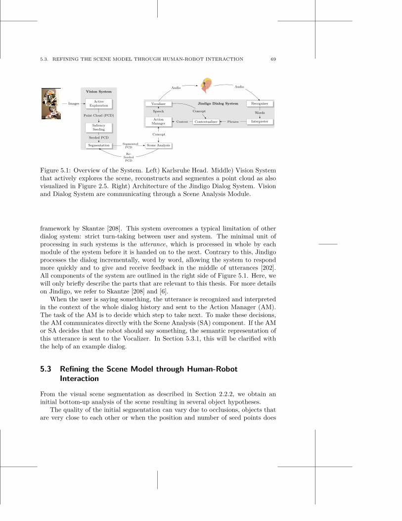
5.3. REFINING THE SCENE MODEL THROUGH HUMAN-ROBOT INTERACTION 69
ActiveExploration
SaliencySeeding
Segmentation
Point Cloud (PCD)
Seeded PCD
Vision System
Images Vocalizer Recognizer
ActionManager Contextualizer Interpreter
Speech Concept Words
PhrasesContext
Audio Audio
Jindigo Dialog System
Scene AnalysisSegmentedPCD
Concept
Re-SeededPCD
Figure 5.1: Overview of the System. Left) Karlsruhe Head. Middle) Vision Systemthat actively explores the scene, reconstructs and segmentes a point cloud as alsovisualized in Figure 2.5. Right) Architecture of the Jindigo Dialog System. Visionand Dialog System are communicating through a Scene Analysis Module.
framework by Skantze [208]. This system overcomes a typical limitation of otherdialog system: strict turn-taking between user and system. The minimal unit ofprocessing in such systems is the utterance, which is processed in whole by eachmodule of the system before it is handed on to the next. Contrary to this, Jindigoprocesses the dialog incrementally, word by word, allowing the system to respondmore quickly and to give and receive feedback in the middle of utterances [202].All components of the system are outlined in the right side of Figure 5.1. Here, wewill only briefly describe the parts that are relevant to this thesis. For more detailson Jindigo, we refer to Skantze [208] and [6].
When the user is saying something, the utterance is recognized and interpretedin the context of the whole dialog history and sent to the Action Manager (AM).The task of the AM is to decide which step to take next. To make these decisions,the AM communicates directly with the Scene Analysis (SA) component. If the AMor SA decides that the robot should say something, the semantic representation ofthis utterance is sent to the Vocalizer. In Section 5.3.1, this will be clarified withthe help of an example dialog.
5.3 Refining the Scene Model through Human-Robot
Interaction
From the visual scene segmentation as described in Section 2.2.2, we obtain aninitial bottom-up analysis of the scene resulting in several object hypotheses.
The quality of the initial segmentation can vary due to occlusions, objects thatare very close to each other or when the position and number of seed points does
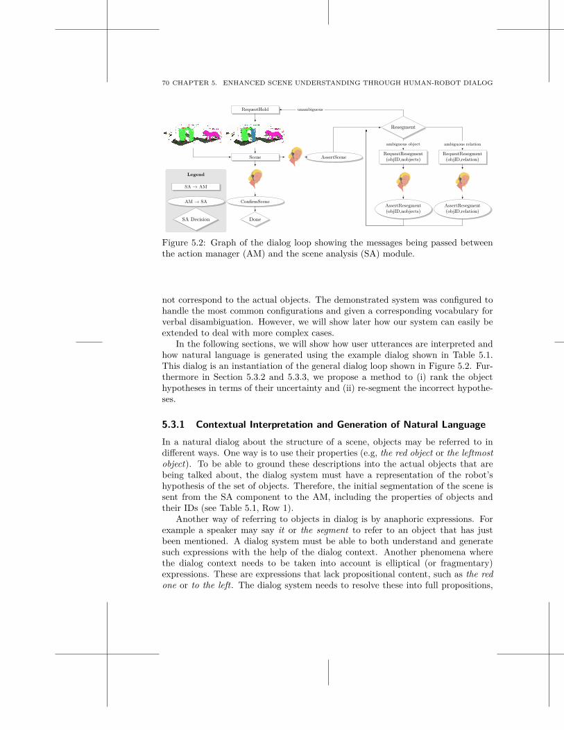
70 CHAPTER 5. ENHANCED SCENE UNDERSTANDING THROUGH HUMAN-ROBOT DIALOG
Scene
RequestHold
AssertScene
Resegment
ConfirmScene
Done
RequestResegment(objID,nobjects)
RequestResegment(objID,relation)
AssertResegment(objID,nobjects)
AssertResegment(objID,relation)
unambiguous
ambiguous relationambiguous object
Legend
SA → AM
AM → SA
SA Decision
Figure 5.2: Graph of the dialog loop showing the messages being passed betweenthe action manager (AM) and the scene analysis (SA) module.
not correspond to the actual objects. The demonstrated system was configured tohandle the most common configurations and given a corresponding vocabulary forverbal disambiguation. However, we will show later how our system can easily beextended to deal with more complex cases.
In the following sections, we will show how user utterances are interpreted andhow natural language is generated using the example dialog shown in Table 5.1.This dialog is an instantiation of the general dialog loop shown in Figure 5.2. Fur-thermore in Section 5.3.2 and 5.3.3, we propose a method to (i) rank the objecthypotheses in terms of their uncertainty and (ii) re-segment the incorrect hypothe-ses.
5.3.1 Contextual Interpretation and Generation of Natural Language
In a natural dialog about the structure of a scene, objects may be referred to indifferent ways. One way is to use their properties (e.g, the red object or the leftmostobject). To be able to ground these descriptions into the actual objects that arebeing talked about, the dialog system must have a representation of the robot’shypothesis of the set of objects. Therefore, the initial segmentation of the scene issent from the SA component to the AM, including the properties of objects andtheir IDs (see Table 5.1, Row 1).
Another way of referring to objects in dialog is by anaphoric expressions. Forexample a speaker may say it or the segment to refer to an object that has justbeen mentioned. A dialog system must be able to both understand and generatesuch expressions with the help of the dialog context. Another phenomena wherethe dialog context needs to be taken into account is elliptical (or fragmentary)expressions. These are expressions that lack propositional content, such as the redone or to the left. The dialog system needs to resolve these into full propositions,
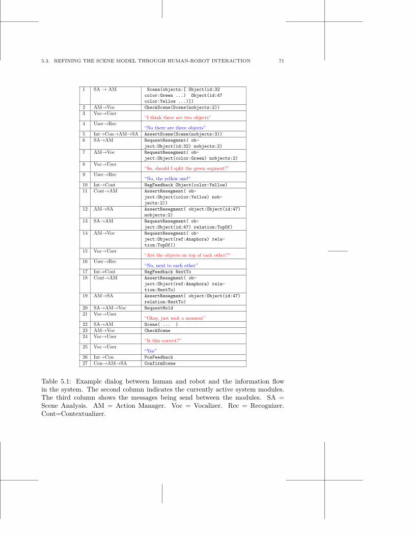
5.3. REFINING THE SCENE MODEL THROUGH HUMAN-ROBOT INTERACTION 71
1 SA → AM Scene(objects:[ Object(id:32
color:Green ...) Object(id:47
color:Yellow ...)])
2 AM→Voc CheckScene(Scene(nobjects:2))
3 Voc→User“I think there are two objects”
4 User→Rec“No there are three objects”
5 Int→Con→AM→SA AssertScene(Scene(nobjects:3))
6 SA→AM RequestResegment( ob-
ject:Object(id:32) nobjects:2)
7 AM→Voc RequestResegment( ob-
ject:Object(color:Green) nobjects:2)
8 Voc→User“So, should I split the green segment?”
9 User→Rec“No, the yellow one!”
10 Int→Cont NegFeedback Object(color:Yellow)
11 Cont→AM AssertResegment( ob-
ject:Object(color:Yellow) nob-
jects:2))
12 AM→SA AssertResegment( object:Object(id:47)
nobjects:2)
13 SA→AM RequestResegment( ob-
ject:Object(id:47) relation:TopOf)
14 AM→Voc RequestResegment( ob-
ject:Object(ref:Anaphora) rela-
tion:TopOf))
15 Voc→User“Are the objects on top of each other?”
16 User→Rec“No, next to each other”
17 Int→Cont NegFeedback NextTo
18 Cont→AM AssertResegment( ob-
ject:Object(ref:Anaphora) rela-
tion:NextTo)
19 AM→SA AssertResegment( object:Object(id:47)
relation:NextTo)
20 SA→AM→Voc RequestHold
21 Voc→User“Okay, just wait a moment”
22 SA→AM Scene( ... )
23 AM→Voc CheckScene
24 Voc→User“Is this correct?”
25 Voc→User“Yes”
26 Int→Con PosFeedback
27 Con→AM→SA ConfirmScene
Table 5.1: Example dialog between human and robot and the information flowin the system. The second column indicates the currently active system modules.The third column shows the messages being send between the modules. SA =Scene Analysis. AM = Action Manager. Voc = Vocalizer. Rec = Recognizer.Cont=Contextualizer.
72 CHAPTER 5. ENHANCED SCENE UNDERSTANDING THROUGH HUMAN-ROBOT DIALOG
so called ellipsis resolution (e.g., the red one should perhaps be understood as thered segment should be split into two objects given the dialog context).
When the AM receives the initial scene, it starts to describe the scene, allowingthe user to correct anything that is incorrect. It starts by stating the number ofobjects using the CheckScene action (Table 5.1, Row 2). This is transformed intotext and speech by the Vocalizer (Row 3). Since the robot’s hypothesis is incorrect,the user now corrects the robot. This utterance is unambiguous and therefore sentas it is all the way to the SA (Row 5). Notice how the semantic representationin Row 2 and 5 and the textual representation in Row 3 and 4 reflect each other.This illustrates how large parts of the domain grammars may be used for bothinterpretation and generation of utterances.
The SA requests help with refining the segment that is most likely to be in-correct (see the next section for how this choice is made). As can be seen in theexample, the SA only refers to objects by their IDs. The AM then chooses the bestway of referring to the object. It may for example be by the color (as in Row 7:the green segment) or by using an anaphoric expression (as in Row 14: the objects)depending on the current dialog history. The user now replies with an elliptical(fragmentary) expression (Row 9). Note that this utterance cannot be fully un-derstood unless the dialog context is taken into account. This is precisely whatthe Contextualizer does - it re-interprets the ellipsis into a full proposition (Row11). Thus, the RequestResegment from the robot combined with the Object fromthe user is transformed into an AssertResegment with this Object as argument.The same principles are applied in the ellipsis resolution in Row 18 (but where thespatial relation is replaced instead of the object).
As the scene is refined, the SA sends new scene hypotheses to the AM (Row22). Finally, it will receive a ConfirmScene message from the AM (Row 27).
5.3.2 Identifying Poor Object Hypotheses through Entropy
To bootstrap the process of scene model refinement, the robot should be able toidentify the most ambiguous object hypotheses and query the user about these first.We propose an entropy-based system to rank the object hypotheses according totheir uncertainty. In general, the entropy H[p(x)] of a distribution over a discreterandom variable x with {x}M
j=0 is defined as follows:
H[P (x)] = −M
∑
j=0
p(xj) ln p(xj). (5.1)
and equivalently for a continuous variable with the integral. Intuitively, this meansthat sharply peaked distributions will have a low entropy while rather flat distri-bution will have a relatively high entropy. The maximum entropy is reached witha uniform distribution and is computed as Hmax[p(x)] = ln (1/M).
Our observation is that single objects tend to be relatively homogeneous in anappropriate attribute space. Consider for example a correctly segmented single
5.3. REFINING THE SCENE MODEL THROUGH HUMAN-ROBOT INTERACTION 73
object and a segment in which two objects are contained as in Figure 5.3. The huehistogram of the correct hypothesis will show a narrower distribution than for thesegment containing two objects. The same holds for the distribution of 3D pointswhich will vary more in the second segment.
To test the hypothesis of entropy being a good indicator for the quality ofobject segmentation, we formalise it as binary classification problem. We computethe entropy for each initial object hypothesis over a number of different attributehistograms. Let N be the set of points in a segment and let us define a set ofnormalized histograms as follows:
1. 1D histogram p(c) with 30 bins over color hue c.
2. 3D histogram pBB(c) over the voxelized BB.
3. 3D histogram p(v) over a voxelized grid (10mm side length) of fixed sizecarrying the number of objects points in each voxel v. The grid is alignedwith the oriented object bounding box BB.
4. One normalized 1D histogram pBBx(s), pBBy
(s), pBBz(s) for each axis x, y
and z of BB.
5. And similarly, one normalized 1D histogram px(s), py(s), pz(s) for each axisx, y and z of the grid of fixed size counting the number of 3D points fallinginto 10mm wide slices s along the respective axis.
For computing the oriented bounding box, we project the segmented point cloudonto the table as for example shown in Figure 4.13. The axes of the boundingbox will be aligned with the two eigenvectors of this projection where ea refers tothe longer and eb to the shorter one. The fixed size grid that is aligned with thisbounding box can for example be chosen dependent on the visible portion of thescene in the foveal cameras.
Both 3D histograms, p(v) and pBB(v), will be relatively sparse compared tothe 1D histograms. While p(v) reflects on the size of an object segment relative towhat is visible in the foveal cameras, pBB(v) is normalized to the dimensions of theoriented bounding box and instead measures the complexity of the 3D distributionof points. The one dimensional histograms break down this complexity to the singleaxes of either the bounding box or the grid.
The entropy values of these histograms are normalized with their respectivemaximum entropy. We use these values to form a feature vector fi containing forexample the following values:
fi = (H[p(C)], H[p(v)], H[pBB(v)], H[px(s)], H[py(s)], H[pz(s)], H[pBBy(s)])
(5.2)
for each object hypothesis i. From a set of initially segmented example scenes, wecan extract labeled data to train an SVM with an RBF kernel for classifying anobject hypothesis as either being correct or not. The probability estimates providedby [50] are used to rank the object hypotheses according to their uncertainty.
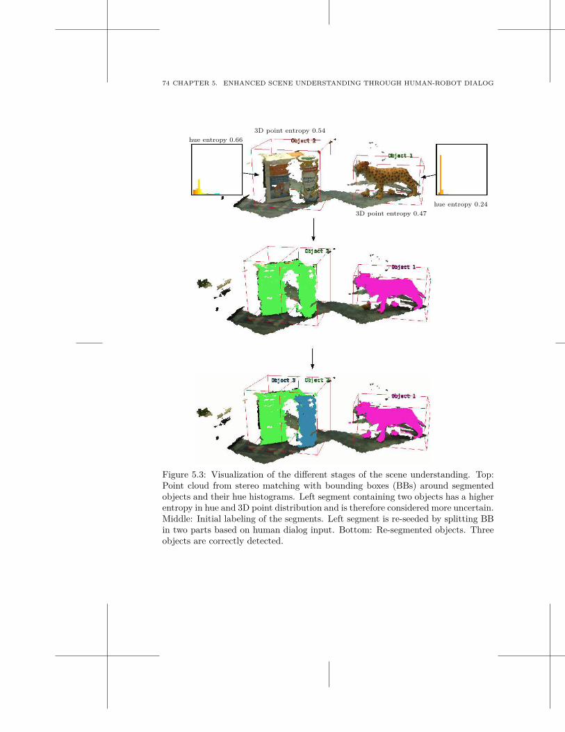
74 CHAPTER 5. ENHANCED SCENE UNDERSTANDING THROUGH HUMAN-ROBOT DIALOG
hue entropy 0.66
3D point entropy 0.54
hue entropy 0.24
3D point entropy 0.47
Figure 5.3: Visualization of the different stages of the scene understanding. Top:Point cloud from stereo matching with bounding boxes (BBs) around segmentedobjects and their hue histograms. Left segment containing two objects has a higherentropy in hue and 3D point distribution and is therefore considered more uncertain.Middle: Initial labeling of the segments. Left segment is re-seeded by splitting BBin two parts based on human dialog input. Bottom: Re-segmented objects. Threeobjects are correctly detected.
5.4. EXPERIMENTS 75
5.3.3 Re-Segmentation Based on User Input
Once a possible candidate for refinement has been identified, the algorithm proceedsto query the user to determine two things: (i) Is the current segmentation correct?And (ii) if not, what is the relative relationships of the objects in the currentincorrect segment. We limit the user’s options for spatial relationships to twoobjects being either next to, in front of or on top of one another. We propose thislimited set of configuration to simplify the interaction. Furthermore, the robustnessof the Markov Random Field (MRF) segmentation algorithm eliminates the needfor tight boundaries. Despite the simplicity of these three rules, quite challengingscenes can be resolved in practice.
To begin the re-segmentation, the extents of the original segment are calculatedto produce an object aligned bounded box. This bounding box is then divided inhalf along one of the three axes based upon the human operator’s input. Oncethe bounding box is divided, the initially segmented points are relabeled and newGaussian Mixture Models for the region are iteratively calculated as in [188]. Anew graph is constructed based on the probability of membership to these newmodels. Energy minimization is performed for the new regions and repeated untilconvergence.
In a similar manner, the more rare situations in which two object hypotheseshave to be merged can be dealt with. The 3D points initially labeled with twodifferent labels would be re-labeled to carry just one.
5.4 Experiments
In this section, we will show that through the interaction of a robot with a humanoperator, the resulting segmentation is improved and that this interaction is mademore efficient through the use of an entropy based selection mechanism.
There exist only a few databases containing RGB-D data, e.g. in [129]. Theyare targeted at object recognition and pose estimation instead of segmentationand usually contain scenes with single objects only. Therefore, we created ourown database by recording 19 scenes containing two to four objects in specificallychallenging configurations, see Figure 5.4. Reconstructing the point cloud andobtaining the seeding for the initial segmentation is done through the active visionsystem described in Section 5.1. An example point cloud for the first scene is shownin Figure 5.3.
In the recorded scenes, objects are hard to separate from each other due tosimilar appearance or close positioning. There is one incorrectly segmented pair ofobjects in each of the 19 scenes. Each scene is labeled with human ground truth,thereby separating each object perfectly.
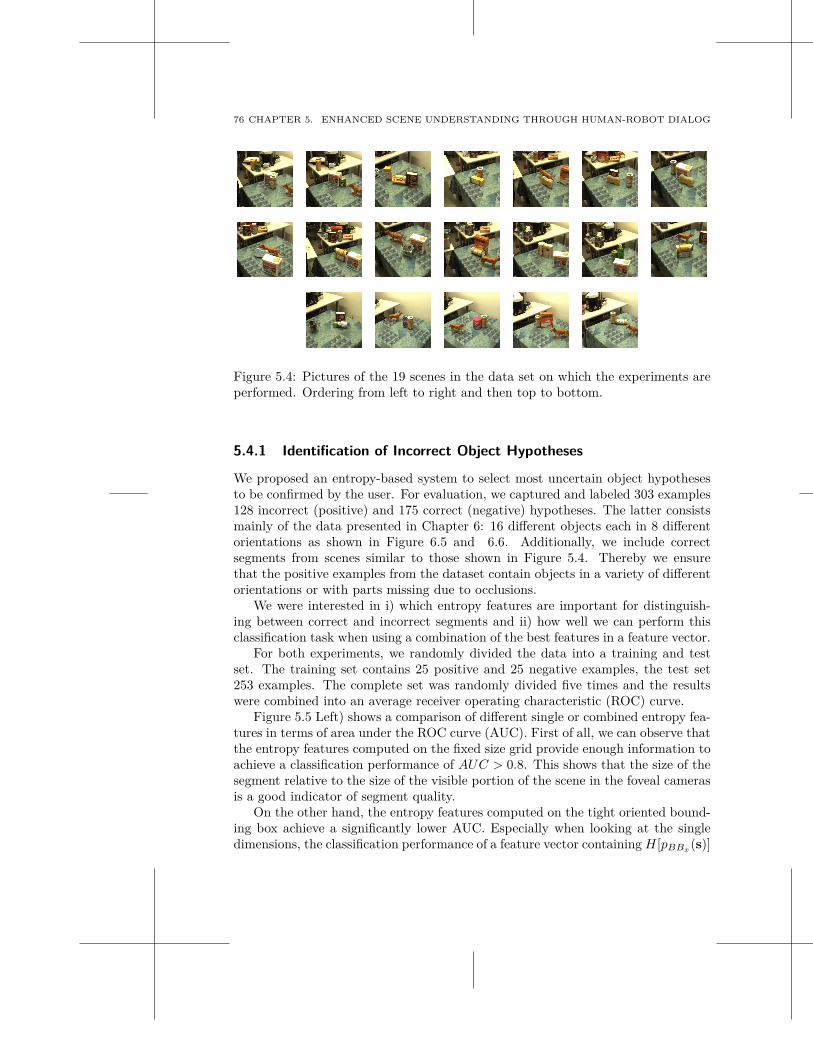
76 CHAPTER 5. ENHANCED SCENE UNDERSTANDING THROUGH HUMAN-ROBOT DIALOG
Figure 5.4: Pictures of the 19 scenes in the data set on which the experiments areperformed. Ordering from left to right and then top to bottom.
5.4.1 Identification of Incorrect Object Hypotheses
We proposed an entropy-based system to select most uncertain object hypothesesto be confirmed by the user. For evaluation, we captured and labeled 303 examples128 incorrect (positive) and 175 correct (negative) hypotheses. The latter consistsmainly of the data presented in Chapter 6: 16 different objects each in 8 differentorientations as shown in Figure 6.5 and 6.6. Additionally, we include correctsegments from scenes similar to those shown in Figure 5.4. Thereby we ensurethat the positive examples from the dataset contain objects in a variety of differentorientations or with parts missing due to occlusions.
We were interested in i) which entropy features are important for distinguish-ing between correct and incorrect segments and ii) how well we can perform thisclassification task when using a combination of the best features in a feature vector.
For both experiments, we randomly divided the data into a training and testset. The training set contains 25 positive and 25 negative examples, the test set253 examples. The complete set was randomly divided five times and the resultswere combined into an average receiver operating characteristic (ROC) curve.
Figure 5.5 Left) shows a comparison of different single or combined entropy fea-tures in terms of area under the ROC curve (AUC). First of all, we can observe thatthe entropy features computed on the fixed size grid provide enough information toachieve a classification performance of AUC > 0.8. This shows that the size of thesegment relative to the size of the visible portion of the scene in the foveal camerasis a good indicator of segment quality.
On the other hand, the entropy features computed on the tight oriented bound-ing box achieve a significantly lower AUC. Especially when looking at the singledimensions, the classification performance of a feature vector containing H[pBBx
(s)]
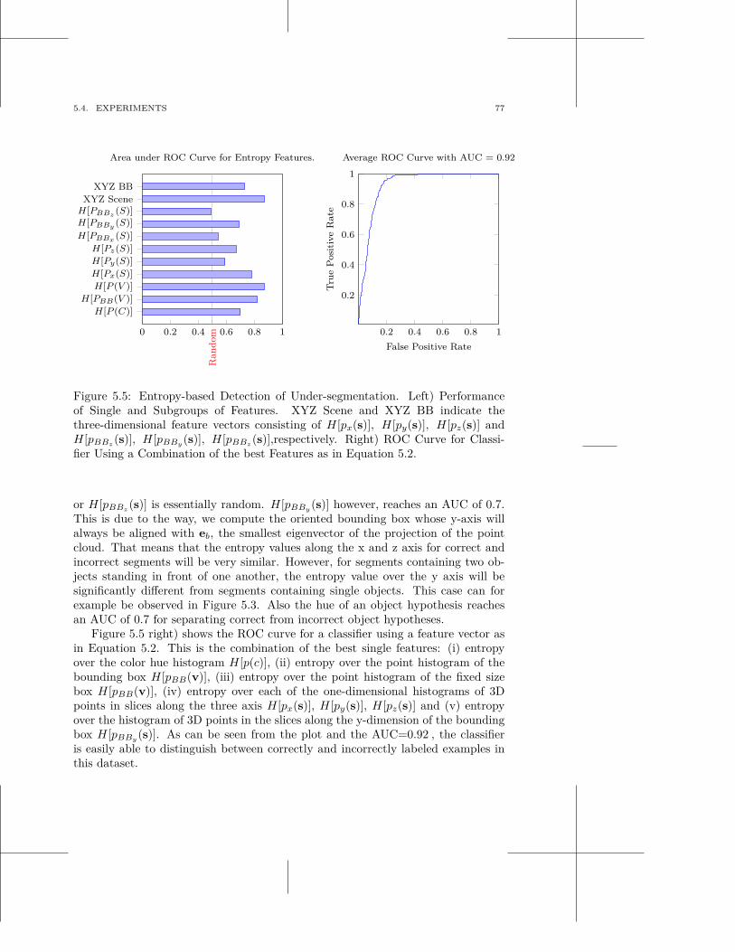
5.4. EXPERIMENTS 77
0 0.2 0.4 0.6 0.8 1
H[P (C)]
H[PBB(V )]
H[P (V )]
H[Px(S)]
H[Py(S)]
H[Pz(S)]
H[PBBx(S)]
H[PBBy(S)]
H[PBBz(S)]
XYZ Scene
XYZ BB
Ran
dom
Area under ROC Curve for Entropy Features.
0.2 0.4 0.6 0.8 1
0.2
0.4
0.6
0.8
1
False Positive Rate
Tru
eP
osi
tive
Rate
Average ROC Curve with AUC = 0.92
Figure 5.5: Entropy-based Detection of Under-segmentation. Left) Performanceof Single and Subgroups of Features. XYZ Scene and XYZ BB indicate thethree-dimensional feature vectors consisting of H[px(s)], H[py(s)], H[pz(s)] andH[pBBz
(s)], H[pBBy(s)], H[pBBz
(s)],respectively. Right) ROC Curve for Classi-fier Using a Combination of the best Features as in Equation 5.2.
or H[pBBz(s)] is essentially random. H[pBBy
(s)] however, reaches an AUC of 0.7.This is due to the way, we compute the oriented bounding box whose y-axis willalways be aligned with eb, the smallest eigenvector of the projection of the pointcloud. That means that the entropy values along the x and z axis for correct andincorrect segments will be very similar. However, for segments containing two ob-jects standing in front of one another, the entropy value over the y axis will besignificantly different from segments containing single objects. This case can forexample be observed in Figure 5.3. Also the hue of an object hypothesis reachesan AUC of 0.7 for separating correct from incorrect object hypotheses.
Figure 5.5 right) shows the ROC curve for a classifier using a feature vector asin Equation 5.2. This is the combination of the best single features: (i) entropyover the color hue histogram H[p(c)], (ii) entropy over the point histogram of thebounding box H[pBB(v)], (iii) entropy over the point histogram of the fixed sizebox H[pBB(v)], (iv) entropy over each of the one-dimensional histograms of 3Dpoints in slices along the three axis H[px(s)], H[py(s)], H[pz(s)] and (v) entropyover the histogram of 3D points in the slices along the y-dimension of the boundingbox H[pBBy
(s)]. As can be seen from the plot and the AUC=0.92 , the classifieris easily able to distinguish between correctly and incorrectly labeled examples inthis dataset.
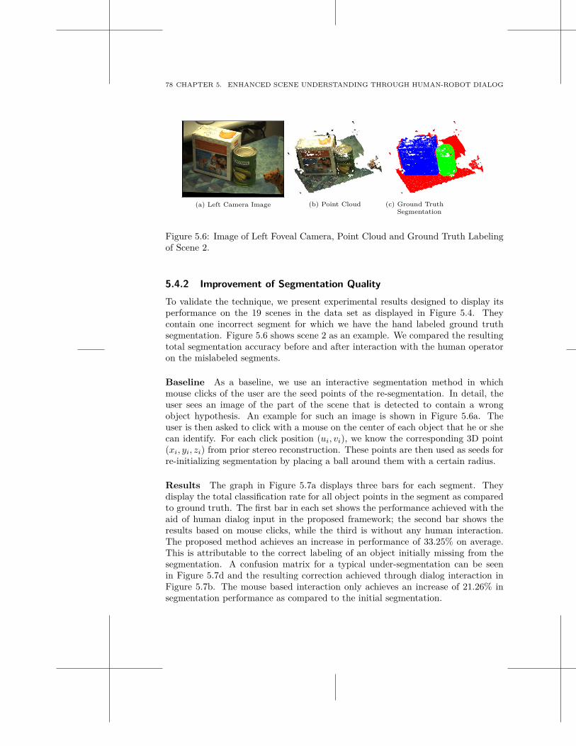
78 CHAPTER 5. ENHANCED SCENE UNDERSTANDING THROUGH HUMAN-ROBOT DIALOG
(a) Left Camera Image (b) Point Cloud (c) Ground TruthSegmentation
Figure 5.6: Image of Left Foveal Camera, Point Cloud and Ground Truth Labelingof Scene 2.
5.4.2 Improvement of Segmentation Quality
To validate the technique, we present experimental results designed to display itsperformance on the 19 scenes in the data set as displayed in Figure 5.4. Theycontain one incorrect segment for which we have the hand labeled ground truthsegmentation. Figure 5.6 shows scene 2 as an example. We compared the resultingtotal segmentation accuracy before and after interaction with the human operatoron the mislabeled segments.
Baseline As a baseline, we use an interactive segmentation method in whichmouse clicks of the user are the seed points of the re-segmentation. In detail, theuser sees an image of the part of the scene that is detected to contain a wrongobject hypothesis. An example for such an image is shown in Figure 5.6a. Theuser is then asked to click with a mouse on the center of each object that he or shecan identify. For each click position (ui, vi), we know the corresponding 3D point(xi, yi, zi) from prior stereo reconstruction. These points are then used as seeds forre-initializing segmentation by placing a ball around them with a certain radius.
Results The graph in Figure 5.7a displays three bars for each segment. Theydisplay the total classification rate for all object points in the segment as comparedto ground truth. The first bar in each set shows the performance achieved with theaid of human dialog input in the proposed framework; the second bar shows theresults based on mouse clicks, while the third is without any human interaction.The proposed method achieves an increase in performance of 33.25% on average.This is attributable to the correct labeling of an object initially missing from thesegmentation. A confusion matrix for a typical under-segmentation can be seenin Figure 5.7d and the resulting correction achieved through dialog interaction inFigure 5.7b. The mouse based interaction only achieves an increase of 21.26% insegmentation performance as compared to the initial segmentation.
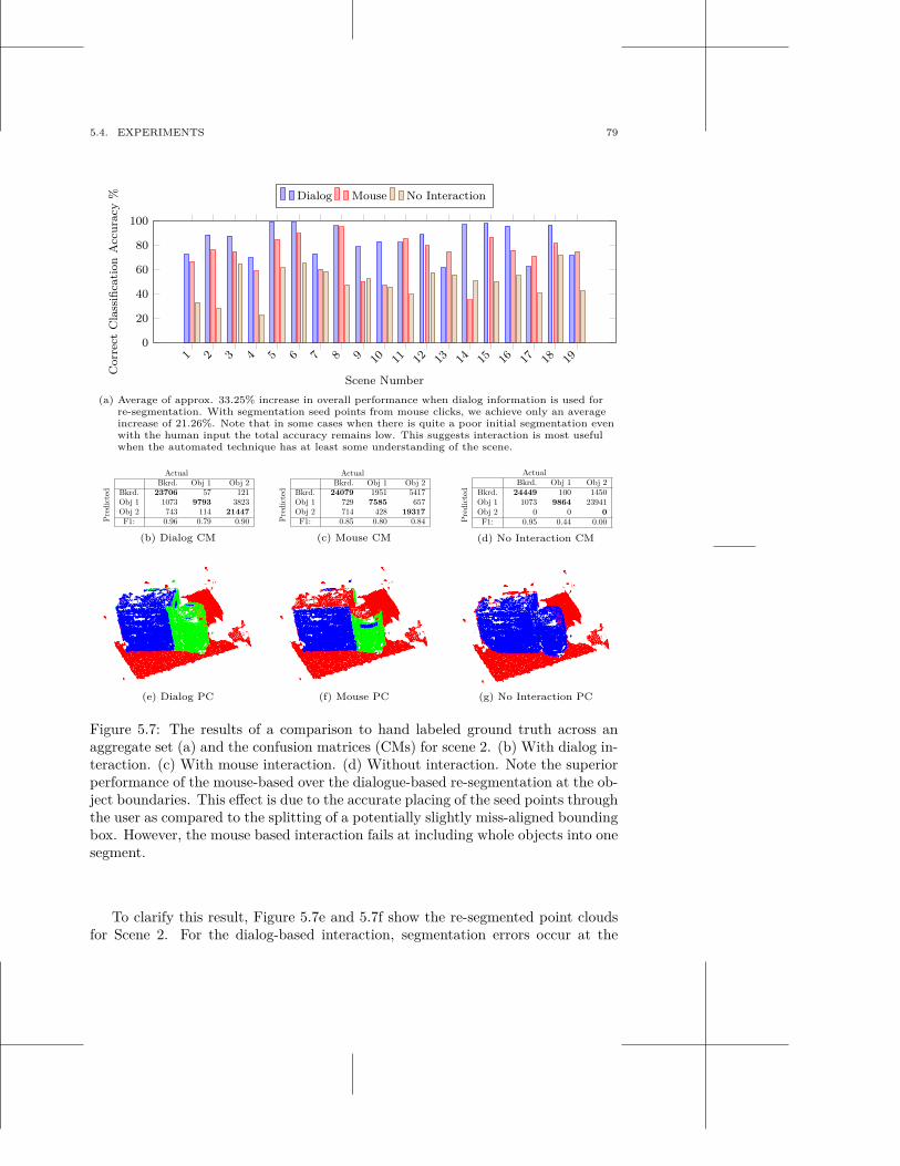
5.4. EXPERIMENTS 79
1 2 3 4 5 6 7 8 9 10 11 12 13 14 15 16 17 18 190
20
40
60
80
100
Scene Number
Corr
ect
Cla
ssifi
cati
on
Acc
ura
cy% Dialog Mouse No Interaction
(a) Average of approx. 33.25% increase in overall performance when dialog information is used forre-segmentation. With segmentation seed points from mouse clicks, we achieve only an averageincrease of 21.26%. Note that in some cases when there is quite a poor initial segmentation evenwith the human input the total accuracy remains low. This suggests interaction is most usefulwhen the automated technique has at least some understanding of the scene.
ActualBkrd. Obj 1 Obj 2
Pre
dict
ed Bkrd. 23706 57 121Obj 1 1073 9793 3823Obj 2 743 114 21447
F1: 0.96 0.79 0.90
(b) Dialog CM
ActualBkrd. Obj 1 Obj 2
Pre
dict
ed Bkrd. 24079 1951 5417Obj 1 729 7585 657Obj 2 714 428 19317
F1: 0.85 0.80 0.84
(c) Mouse CM
ActualBkrd. Obj 1 Obj 2
Pre
dict
ed Bkrd. 24449 100 1450Obj 1 1073 9864 23941Obj 2 0 0 0
F1: 0.95 0.44 0.00
(d) No Interaction CM
(e) Dialog PC (f) Mouse PC (g) No Interaction PC
Figure 5.7: The results of a comparison to hand labeled ground truth across anaggregate set (a) and the confusion matrices (CMs) for scene 2. (b) With dialog in-teraction. (c) With mouse interaction. (d) Without interaction. Note the superiorperformance of the mouse-based over the dialogue-based re-segmentation at the ob-ject boundaries. This effect is due to the accurate placing of the seed points throughthe user as compared to the splitting of a potentially slightly miss-aligned boundingbox. However, the mouse based interaction fails at including whole objects into onesegment.
To clarify this result, Figure 5.7e and 5.7f show the re-segmented point cloudsfor Scene 2. For the dialog-based interaction, segmentation errors occur at the
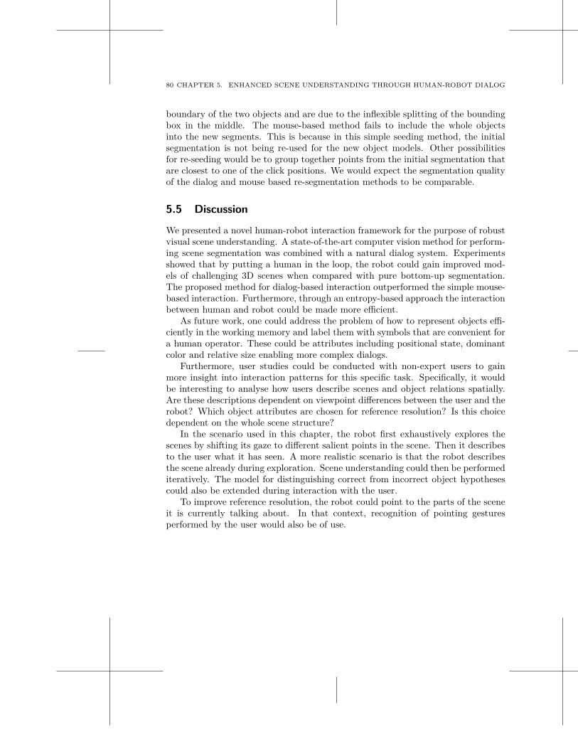
80 CHAPTER 5. ENHANCED SCENE UNDERSTANDING THROUGH HUMAN-ROBOT DIALOG
boundary of the two objects and are due to the inflexible splitting of the boundingbox in the middle. The mouse-based method fails to include the whole objectsinto the new segments. This is because in this simple seeding method, the initialsegmentation is not being re-used for the new object models. Other possibilitiesfor re-seeding would be to group together points from the initial segmentation thatare closest to one of the click positions. We would expect the segmentation qualityof the dialog and mouse based re-segmentation methods to be comparable.
5.5 Discussion
We presented a novel human-robot interaction framework for the purpose of robustvisual scene understanding. A state-of-the-art computer vision method for perform-ing scene segmentation was combined with a natural dialog system. Experimentsshowed that by putting a human in the loop, the robot could gain improved mod-els of challenging 3D scenes when compared with pure bottom-up segmentation.The proposed method for dialog-based interaction outperformed the simple mouse-based interaction. Furthermore, through an entropy-based approach the interactionbetween human and robot could be made more efficient.
As future work, one could address the problem of how to represent objects effi-ciently in the working memory and label them with symbols that are convenient fora human operator. These could be attributes including positional state, dominantcolor and relative size enabling more complex dialogs.
Furthermore, user studies could be conducted with non-expert users to gainmore insight into interaction patterns for this specific task. Specifically, it wouldbe interesting to analyse how users describe scenes and object relations spatially.Are these descriptions dependent on viewpoint differences between the user and therobot? Which object attributes are chosen for reference resolution? Is this choicedependent on the whole scene structure?
In the scenario used in this chapter, the robot first exhaustively explores thescenes by shifting its gaze to different salient points in the scene. Then it describesto the user what it has seen. A more realistic scenario is that the robot describesthe scene already during exploration. Scene understanding could then be performediteratively. The model for distinguishing correct from incorrect object hypothesescould also be extended during interaction with the user.
To improve reference resolution, the robot could point to the parts of the sceneit is currently talking about. In that context, recognition of pointing gesturesperformed by the user would also be of use.
6
Predicting Unknown Object Shape
Many challenging problems addressed by the robotics community are currentlystudied in simulation. Examples are motion planning [125, 66, 225] or grasp plan-ning [53, 90, 153] in which the knowledge of the complete world model or of specificobjects is assumed to be known. However, on a real robotic platform this assump-tion breaks down due to noisy sensors or occlusions.
Consider for example the point cloud in Figure 6.1 that was reconstructed withan active stereo head from a table-top scene. Due to occlusions, no informationabout the backside of the object or about the region behind it is available from purestereo reconstructed data. There are gaps in the scene and object representations.Additionally, noise causes the observed 3D structure of an object or scene to deviatefrom its true shape. Although the previously mentioned planners might be appliedon real robotic platforms, a mismatch between the real world and the world modelis usually not taken into account explicitly.
Exceptions are reactive grasping strategies that adapt their behavior based onsensor data generated during execution time [78, 98, 99].
In this section, we consider the problem of picking up objects from a table-topscene containing several objects. We assume that the robot has reconstructed apoint cloud from the scene using the approach from Section 2.2.1. Additionally, we
Figure 6.1: How can a suitable grasp pose be determined based on an incompletepoint cloud? Left and Middle) Example views of a raw stereo reconstructed pointcloud. Right) Model of the Schunk Hand with some of its degrees of freedom.
81
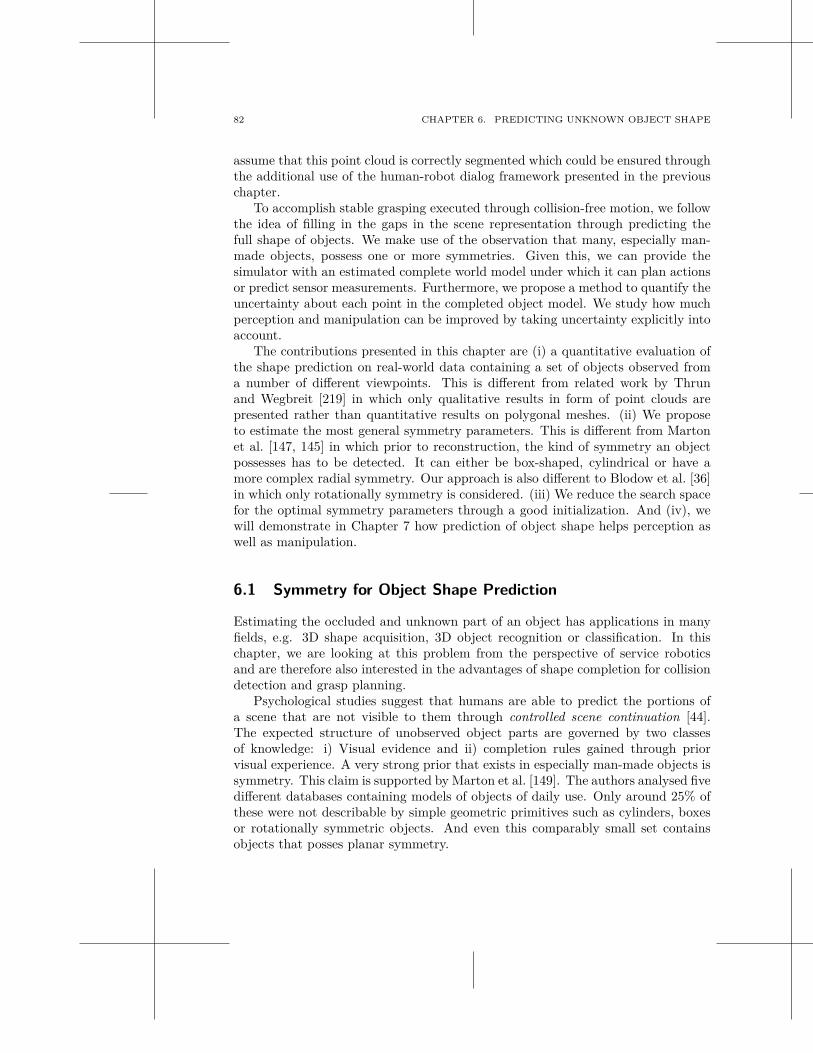
82 CHAPTER 6. PREDICTING UNKNOWN OBJECT SHAPE
assume that this point cloud is correctly segmented which could be ensured throughthe additional use of the human-robot dialog framework presented in the previouschapter.
To accomplish stable grasping executed through collision-free motion, we followthe idea of filling in the gaps in the scene representation through predicting thefull shape of objects. We make use of the observation that many, especially man-made objects, possess one or more symmetries. Given this, we can provide thesimulator with an estimated complete world model under which it can plan actionsor predict sensor measurements. Furthermore, we propose a method to quantify theuncertainty about each point in the completed object model. We study how muchperception and manipulation can be improved by taking uncertainty explicitly intoaccount.
The contributions presented in this chapter are (i) a quantitative evaluation ofthe shape prediction on real-world data containing a set of objects observed froma number of different viewpoints. This is different from related work by Thrunand Wegbreit [219] in which only qualitative results in form of point clouds arepresented rather than quantitative results on polygonal meshes. (ii) We proposeto estimate the most general symmetry parameters. This is different from Martonet al. [147, 145] in which prior to reconstruction, the kind of symmetry an objectpossesses has to be detected. It can either be box-shaped, cylindrical or have amore complex radial symmetry. Our approach is also different to Blodow et al. [36]in which only rotationally symmetry is considered. (iii) We reduce the search spacefor the optimal symmetry parameters through a good initialization. And (iv), wewill demonstrate in Chapter 7 how prediction of object shape helps perception aswell as manipulation.
6.1 Symmetry for Object Shape Prediction
Estimating the occluded and unknown part of an object has applications in manyfields, e.g. 3D shape acquisition, 3D object recognition or classification. In thischapter, we are looking at this problem from the perspective of service roboticsand are therefore also interested in the advantages of shape completion for collisiondetection and grasp planning.
Psychological studies suggest that humans are able to predict the portions ofa scene that are not visible to them through controlled scene continuation [44].The expected structure of unobserved object parts are governed by two classesof knowledge: i) Visual evidence and ii) completion rules gained through priorvisual experience. A very strong prior that exists in especially man-made objects issymmetry. This claim is supported by Marton et al. [149]. The authors analysed fivedifferent databases containing models of objects of daily use. Only around 25% ofthese were not describable by simple geometric primitives such as cylinders, boxesor rotationally symmetric objects. And even this comparably small set containsobjects that posses planar symmetry.
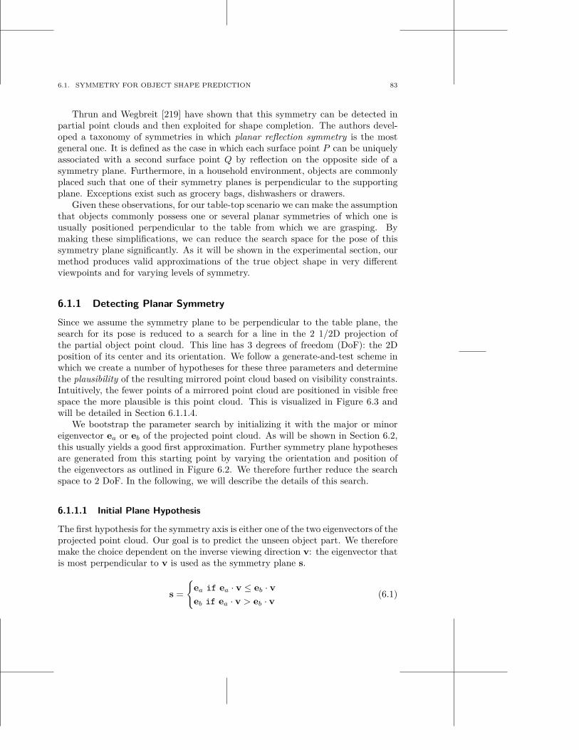
6.1. SYMMETRY FOR OBJECT SHAPE PREDICTION 83
Thrun and Wegbreit [219] have shown that this symmetry can be detected inpartial point clouds and then exploited for shape completion. The authors devel-oped a taxonomy of symmetries in which planar reflection symmetry is the mostgeneral one. It is defined as the case in which each surface point P can be uniquelyassociated with a second surface point Q by reflection on the opposite side of asymmetry plane. Furthermore, in a household environment, objects are commonlyplaced such that one of their symmetry planes is perpendicular to the supportingplane. Exceptions exist such as grocery bags, dishwashers or drawers.
Given these observations, for our table-top scenario we can make the assumptionthat objects commonly possess one or several planar symmetries of which one isusually positioned perpendicular to the table from which we are grasping. Bymaking these simplifications, we can reduce the search space for the pose of thissymmetry plane significantly. As it will be shown in the experimental section, ourmethod produces valid approximations of the true object shape in very differentviewpoints and for varying levels of symmetry.
6.1.1 Detecting Planar Symmetry
Since we assume the symmetry plane to be perpendicular to the table plane, thesearch for its pose is reduced to a search for a line in the 2 1/2D projection ofthe partial object point cloud. This line has 3 degrees of freedom (DoF): the 2Dposition of its center and its orientation. We follow a generate-and-test scheme inwhich we create a number of hypotheses for these three parameters and determinethe plausibility of the resulting mirrored point cloud based on visibility constraints.Intuitively, the fewer points of a mirrored point cloud are positioned in visible freespace the more plausible is this point cloud. This is visualized in Figure 6.3 andwill be detailed in Section 6.1.1.4.
We bootstrap the parameter search by initializing it with the major or minoreigenvector ea or eb of the projected point cloud. As will be shown in Section 6.2,this usually yields a good first approximation. Further symmetry plane hypothesesare generated from this starting point by varying the orientation and position ofthe eigenvectors as outlined in Figure 6.2. We therefore further reduce the searchspace to 2 DoF. In the following, we will describe the details of this search.
6.1.1.1 Initial Plane Hypothesis
The first hypothesis for the symmetry axis is either one of the two eigenvectors of theprojected point cloud. Our goal is to predict the unseen object part. We thereforemake the choice dependent on the inverse viewing direction v: the eigenvector thatis most perpendicular to v is used as the symmetry plane s.
s =
{
ea if ea · v ≤ eb · v
eb if ea · v > eb · v(6.1)
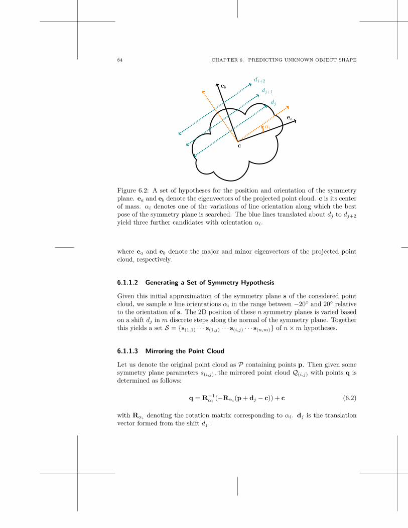
84 CHAPTER 6. PREDICTING UNKNOWN OBJECT SHAPE
ea
eb
c
αi
dj
dj+1
dj+2
Figure 6.2: A set of hypotheses for the position and orientation of the symmetryplane. ea and eb denote the eigenvectors of the projected point cloud. c is its centerof mass. αi denotes one of the variations of line orientation along which the bestpose of the symmetry plane is searched. The blue lines translated about dj to dj+2
yield three further candidates with orientation αi.
where ea and eb denote the major and minor eigenvectors of the projected pointcloud, respectively.
6.1.1.2 Generating a Set of Symmetry Hypothesis
Given this initial approximation of the symmetry plane s of the considered pointcloud, we sample n line orientations αi in the range between −20◦ and 20◦ relativeto the orientation of s. The 2D position of these n symmetry planes is varied basedon a shift dj in m discrete steps along the normal of the symmetry plane. Togetherthis yields a set S = {s(1,1) · · · s(1,j) · · · s(i,j) · · · s(n,m)} of n × m hypotheses.
6.1.1.3 Mirroring the Point Cloud
Let us denote the original point cloud as P containing points p. Then given somesymmetry plane parameters s(i,j), the mirrored point cloud Q(i,j) with points q isdetermined as follows:
q = R−1αi
(−Rαi(p + dj − c)) + c (6.2)
with Rαidenoting the rotation matrix corresponding to αi. dj is the translation
vector formed from the shift dj .
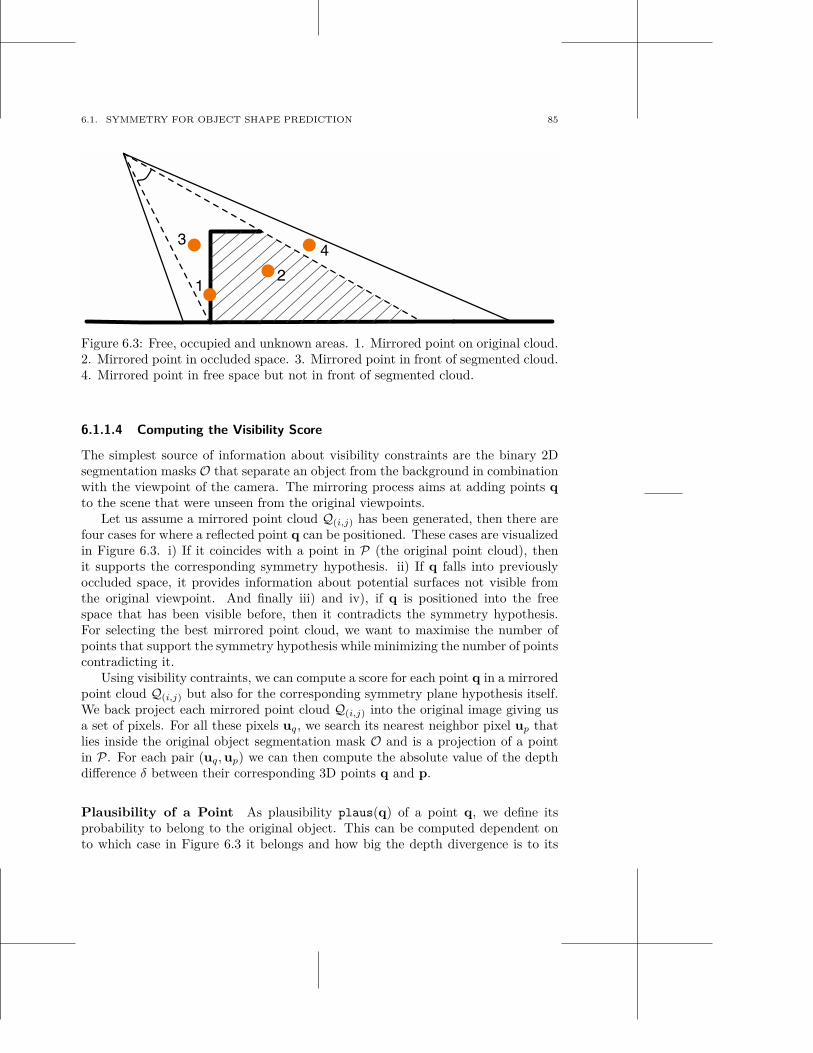
6.1. SYMMETRY FOR OBJECT SHAPE PREDICTION 85
1
3
2
4
Figure 6.3: Free, occupied and unknown areas. 1. Mirrored point on original cloud.2. Mirrored point in occluded space. 3. Mirrored point in front of segmented cloud.4. Mirrored point in free space but not in front of segmented cloud.
6.1.1.4 Computing the Visibility Score
The simplest source of information about visibility constraints are the binary 2Dsegmentation masks O that separate an object from the background in combinationwith the viewpoint of the camera. The mirroring process aims at adding points q
to the scene that were unseen from the original viewpoints.Let us assume a mirrored point cloud Q(i,j) has been generated, then there are
four cases for where a reflected point q can be positioned. These cases are visualizedin Figure 6.3. i) If it coincides with a point in P (the original point cloud), thenit supports the corresponding symmetry hypothesis. ii) If q falls into previouslyoccluded space, it provides information about potential surfaces not visible fromthe original viewpoint. And finally iii) and iv), if q is positioned into the freespace that has been visible before, then it contradicts the symmetry hypothesis.For selecting the best mirrored point cloud, we want to maximise the number ofpoints that support the symmetry hypothesis while minimizing the number of pointscontradicting it.
Using visibility contraints, we can compute a score for each point q in a mirroredpoint cloud Q(i,j) but also for the corresponding symmetry plane hypothesis itself.We back project each mirrored point cloud Q(i,j) into the original image giving usa set of pixels. For all these pixels uq, we search its nearest neighbor pixel up thatlies inside the original object segmentation mask O and is a projection of a pointin P. For each pair (uq, up) we can then compute the absolute value of the depthdifference δ between their corresponding 3D points q and p.
Plausibility of a Point As plausibility plaus(q) of a point q, we define itsprobability to belong to the original object. This can be computed dependent onto which case in Figure 6.3 it belongs and how big the depth divergence is to its
86 CHAPTER 6. PREDICTING UNKNOWN OBJECT SHAPE
nearest neighbor in P. For all points q falling into the occluded space or coincidewith the segmented object as in case one and two of Figure 6.3, we compute
plaus1(q) =δ × (0.5 − plausmax)
δmax+ plausmax (6.3)
where plausmax refers to the maximum plausibility and δmax to the maximumdepth divergence. Each point in the occluded space will have a minimum probabilityto belong to the real object of 0.5. The higher the depth divergence δ of a point toits nearest neighbor, the lower will be its plausibility. This relationship is definedas a linear fall-off.
For all points q falling into previously visible space (case three and four inFigure 6.3), we similarly compute their plausibility as
plaus2(q) =−δ × plausmax
δmax+ plausmax. (6.4)
In contrast to Equation 6.3, Equation 6.4 can assign 0 as the minimum probabilityof a point to belong to the object. All original points p of the point cloud will haveplausmax assigned which can be lower than 1 to account for noise.
Plausibility of a whole point cloud The plausibility score p(i,j) for the wholemirrored point cloud Q(i,j), i.e., the symmetry plane hypothesis s(i,j) consists of twoparts each reflecting the third or fourth case as visualized in Figure 6.3. Let q /∈ Orefer to all points whose projection does not fall into the original segmentation maskO. And let q ∈ O refer to the set of points whose projections falls into O. Thenp(i,j) is computed as the sum of expected values of the plausibilities in these twosets:
p(i,j) = IEq/∈O [plaus2(q)] + IEq∈O[plaus2(q)]. (6.5)
In case the plane parameters are chosen such that there is a large overlap betweenthe original point cloud P and the mirrored cloud Q(i,j), the second part of Equa-tion 6.5 will be relatively large compared to the first part. The bigger dj , i.e. shiftof the symmetry plane as visualized in Figure 6.2, IEq∈O [plaus2(q)] will increaseand IEq/∈O[plaus2(q)] decrease. We are searching for symmetry plane parameterss(i,j) that produce a mirrored point cloud with a global maximum in the space ofthe plausibilities scores
s∗(i,j) = arg max
Sp(i,j). (6.6)
The corresponding Q(i,j) will have the smallest amount of points contradicting thesymmetry hypothesis and therefore is of a maximum plausibility.
6.1.2 Surface Approximation of Completed Point Clouds
After the prediction of the backside of an object point cloud, we want to createa surface mesh approximation to support grasp planning and collision detection.
6.1. SYMMETRY FOR OBJECT SHAPE PREDICTION 87
We use Poisson surface reconstruction for this purpose proposed by Kazhdan et al.[113]. This method is a global method considering all data at once. It producessmooth watertight surfaces that robustly approximate noisy data.
6.1.2.1 Introduction to Poisson Surface Reconstruction
Poisson surface reconstruction approaches the problem by computing an indicatorfunction X that takes the value 1 at points inside the object and 0 outside of it.The reconstructed surface then equals an appropriate iso-surface. The key insightused for formulating surface reconstruction as a poisson problem is that there is aclose relationship between a set of oriented points sampled from the real surface andX . Specifically, the gradient ∇X of the indicator function is 0 almost everywhereexcept from close to the surface where it equals the inward surface normals. Theset of oriented points S can therefore be seen as samples from ∇X . Computingthe indicator function can then be formulated as finding X whose gradient bestapproximates a vector field ~V as defined by the points in S.
X = minX
||∇X − ~V|| (6.7)
To convert this into a standard poisson problem, Kazhdan et al. [113] proposeto find the least-squares approximate solution of the indicator function X whosesecond derivative equals the first derivative of the vector field ~V.
∆X ≡ ∇∇X = ∇~V (6.8)
For details on how this is efficiently solved, we refer to [113]. Here, we will concen-trate on the aspects that are relevant to this thesis.
Given point samples S and a desired tree depth D, an adaptive octree is definedin which each sample falls into a leaf node at D. A function fo(·) is associated witheach node o in that tree. It maps a sample point q from the set S to a scalar valuesuch that the indicator function can be precisely and efficiently evaluated near thesample points. In [113] fo is chosen to be an approximation of a unit-varianceGaussian centered about the node o and stretched by its size.
To achieve subnode precision in the vector field, trilinear interpolation is usedto distribute a sample across its nearest neighbor nodes at depth D.
~V(q) ≡∑
s∈S
∑
o∈NgbrD(s)
αo,sfo(q)ns (6.9)
where αo,s are the appropriate weights for interpolation and ns the normal of thesample s.
To choose the appropriate iso-value γ at which the iso-surface δM is extracted,X is evaluated at all the samples from set S. The average of the resulting values isthen used as the iso-value.
δM ≡ {q ∈ IR3|X (q) = γ} (6.10)
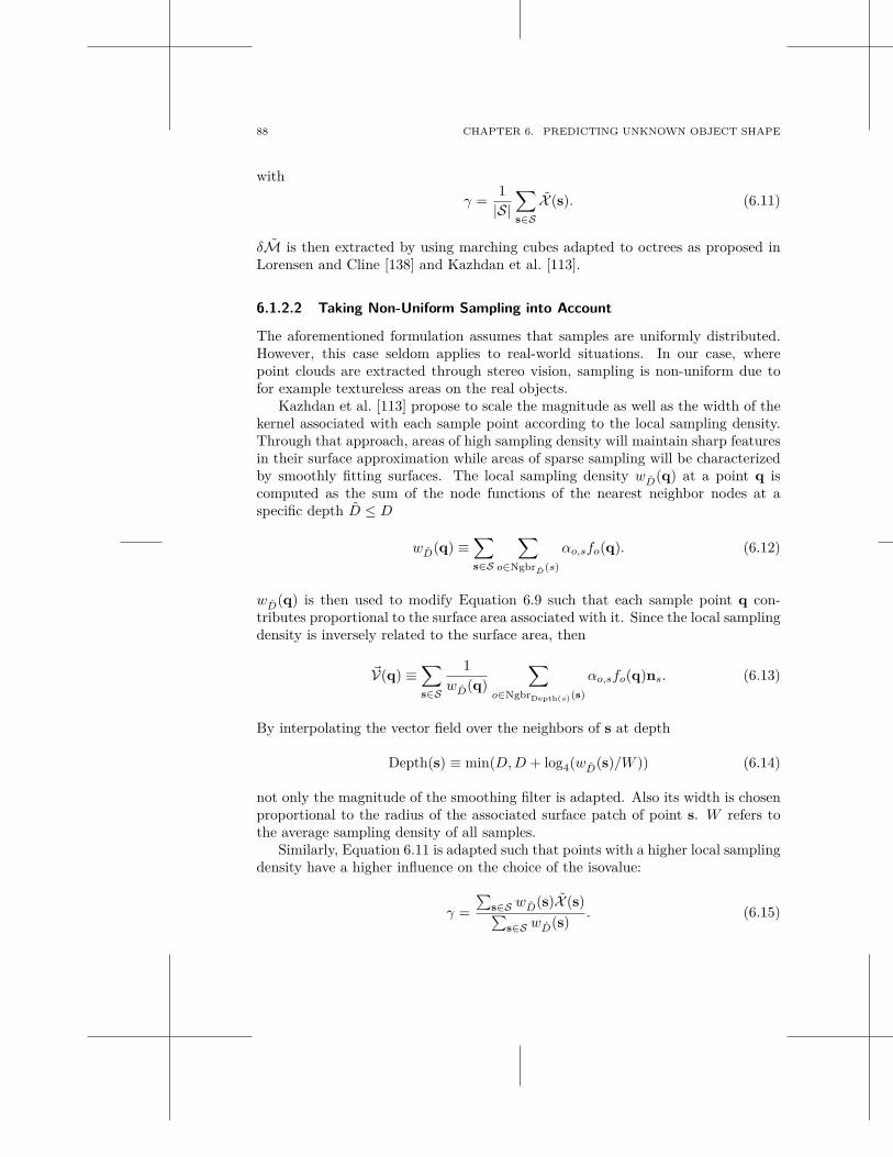
88 CHAPTER 6. PREDICTING UNKNOWN OBJECT SHAPE
with
γ =1
|S|∑
s∈S
X (s). (6.11)
δM is then extracted by using marching cubes adapted to octrees as proposed inLorensen and Cline [138] and Kazhdan et al. [113].
6.1.2.2 Taking Non-Uniform Sampling into Account
The aforementioned formulation assumes that samples are uniformly distributed.However, this case seldom applies to real-world situations. In our case, wherepoint clouds are extracted through stereo vision, sampling is non-uniform due tofor example textureless areas on the real objects.
Kazhdan et al. [113] propose to scale the magnitude as well as the width of thekernel associated with each sample point according to the local sampling density.Through that approach, areas of high sampling density will maintain sharp featuresin their surface approximation while areas of sparse sampling will be characterizedby smoothly fitting surfaces. The local sampling density wD(q) at a point q iscomputed as the sum of the node functions of the nearest neighbor nodes at aspecific depth D ≤ D
wD(q) ≡∑
s∈S
∑
o∈NgbrD
(s)
αo,sfo(q). (6.12)
wD(q) is then used to modify Equation 6.9 such that each sample point q con-tributes proportional to the surface area associated with it. Since the local samplingdensity is inversely related to the surface area, then
~V(q) ≡∑
s∈S
1wD(q)
∑
o∈NgbrDepth(s)(s)
αo,sfo(q)ns. (6.13)
By interpolating the vector field over the neighbors of s at depth
Depth(s) ≡ min(D, D + log4(wD(s)/W )) (6.14)
not only the magnitude of the smoothing filter is adapted. Also its width is chosenproportional to the radius of the associated surface patch of point s. W refers tothe average sampling density of all samples.
Similarly, Equation 6.11 is adapted such that points with a higher local samplingdensity have a higher influence on the choice of the isovalue:
γ =
∑
s∈S wD(s)X (s)∑
s∈S wD(s). (6.15)
6.1. SYMMETRY FOR OBJECT SHAPE PREDICTION 89
6.1.2.3 Plausibility for Improved Robustness of the Surface Reconstruction
Kazhdan et al. [113] propose to adapt their approach to take confidence value ofthe sampling points into account which is implemented in [112]. In this thesis, wewant to show that different prediction mechanisms are useful for improving percep-tion but also manipulation and grasping. Additionally, we have already shown inSection 4 that having an idea about the uncertainty in a prediction helps to effi-ciently explore a scene. In this section, we want to show that using the probabilityof a point in the mirrored point cloud to be from the original object improves therobustness of surface reconstruction. This probability is defined as the plausibilityplaus(q) of a point q according to visibility constraints as in Equation 6.3 and 6.4.
The intuition behind the following adaptation of the poisson equations is thatsample points with low plausibility do not need to be represented with fine detail.Equation 6.13 is therefore adapted as follows
~V(q) ≡∑
s∈S
1wD(q) · plaus(q)
∑
o∈NgbrDepth(s)(s)
αo,sfo(q)ns. (6.16)
whereDepth(s) ≡ min(D, D + log4(wD(s) · plaus(s)/W )) (6.17)
Equation 6.11 is adapted as follows:
γ =
∑
s∈S wD(s) · plaus(s)X (s)∑
s∈S wD(s · plaus(s)). (6.18)
As will be shown in Section 6.2, this is specifically beneficial at the seams of thecompleted point cloud where old and new points overlap. These places are proneto noise and potentially contradictory normal information. New points that tendto have a lower plausibility than old points should therefore be down-weighted toachieve smooth boundaries.
6.1.2.4 Computing the Normals of the Completed Point Cloud
The point cloud data, that we use as sample set S is not originally oriented. Todetermine the normals, we use a kd-tree as proposed by Hoppe et al. [97]. A localplane fit is estimated for the k-nearest neighbors of the target point. This planeis assumed to be a local approximation of the surface at the current point. Moreadvanced normal estimation techniques as for example by Cole et al. [54] and Mitraand Nguyen [154] have been proposed which could perhaps increase the performanceof the surface reconstruction at the cost of computation speed. Following normalestimation, we ensure that the normals of the mirrored points are consistent withthe mirrored viewing direction reflected across the plane of symmetry.
It should be noted while Poisson surface reconstruction is robust to some noise,it is sensitive to normal direction. We therefore filter outliers from the segmented
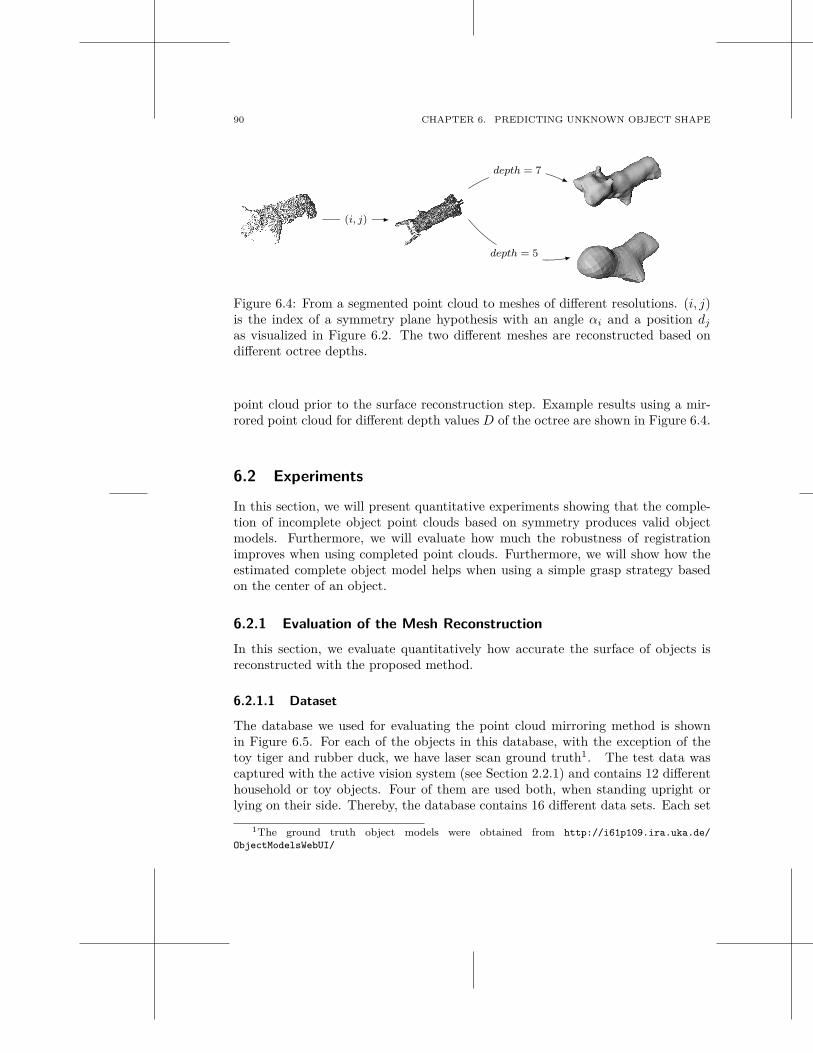
90 CHAPTER 6. PREDICTING UNKNOWN OBJECT SHAPE
(i, j)
depth = 5
depth = 7
Figure 6.4: From a segmented point cloud to meshes of different resolutions. (i, j)is the index of a symmetry plane hypothesis with an angle αi and a position dj
as visualized in Figure 6.2. The two different meshes are reconstructed based ondifferent octree depths.
point cloud prior to the surface reconstruction step. Example results using a mir-rored point cloud for different depth values D of the octree are shown in Figure 6.4.
6.2 Experiments
In this section, we will present quantitative experiments showing that the comple-tion of incomplete object point clouds based on symmetry produces valid objectmodels. Furthermore, we will evaluate how much the robustness of registrationimproves when using completed point clouds. Furthermore, we will show how theestimated complete object model helps when using a simple grasp strategy basedon the center of an object.
6.2.1 Evaluation of the Mesh Reconstruction
In this section, we evaluate quantitatively how accurate the surface of objects isreconstructed with the proposed method.
6.2.1.1 Dataset
The database we used for evaluating the point cloud mirroring method is shownin Figure 6.5. For each of the objects in this database, with the exception of thetoy tiger and rubber duck, we have laser scan ground truth1. The test data wascaptured with the active vision system (see Section 2.2.1) and contains 12 differenthousehold or toy objects. Four of them are used both, when standing upright orlying on their side. Thereby, the database contains 16 different data sets. Each set
1The ground truth object models were obtained from http://i61p109.ira.uka.de/
ObjectModelsWebUI/
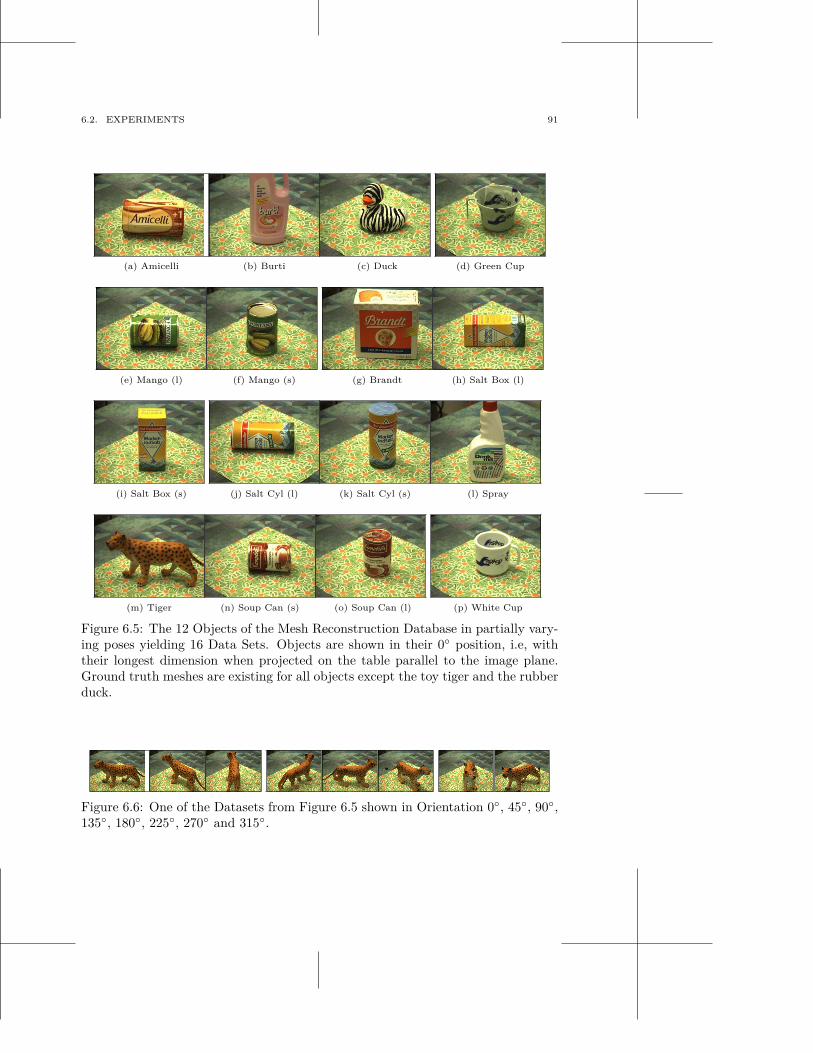
6.2. EXPERIMENTS 91
(a) Amicelli (b) Burti (c) Duck (d) Green Cup
(e) Mango (l) (f) Mango (s) (g) Brandt (h) Salt Box (l)
(i) Salt Box (s) (j) Salt Cyl (l) (k) Salt Cyl (s) (l) Spray
(m) Tiger (n) Soup Can (s) (o) Soup Can (l) (p) White Cup
Figure 6.5: The 12 Objects of the Mesh Reconstruction Database in partially vary-ing poses yielding 16 Data Sets. Objects are shown in their 0◦ position, i.e, withtheir longest dimension when projected on the table parallel to the image plane.Ground truth meshes are existing for all objects except the toy tiger and the rubberduck.
Figure 6.6: One of the Datasets from Figure 6.5 shown in Orientation 0◦, 45◦, 90◦,135◦, 180◦, 225◦, 270◦ and 315◦.
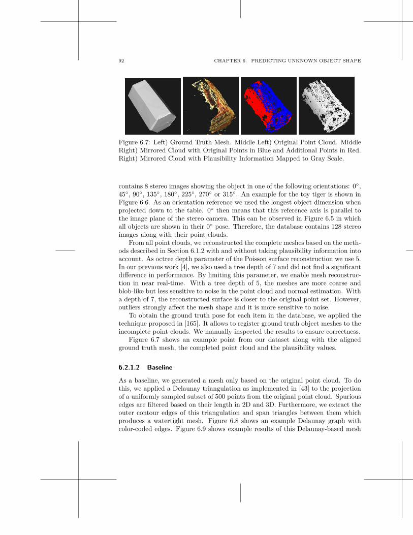
92 CHAPTER 6. PREDICTING UNKNOWN OBJECT SHAPE
Figure 6.7: Left) Ground Truth Mesh. Middle Left) Original Point Cloud. MiddleRight) Mirrored Cloud with Original Points in Blue and Additional Points in Red.Right) Mirrored Cloud with Plausibility Information Mapped to Gray Scale.
contains 8 stereo images showing the object in one of the following orientations: 0◦,45◦, 90◦, 135◦, 180◦, 225◦, 270◦ or 315◦. An example for the toy tiger is shown inFigure 6.6. As an orientation reference we used the longest object dimension whenprojected down to the table. 0◦ then means that this reference axis is parallel tothe image plane of the stereo camera. This can be observed in Figure 6.5 in whichall objects are shown in their 0◦ pose. Therefore, the database contains 128 stereoimages along with their point clouds.
From all point clouds, we reconstructed the complete meshes based on the meth-ods described in Section 6.1.2 with and without taking plausibility information intoaccount. As octree depth parameter of the Poisson surface reconstruction we use 5.In our previous work [4], we also used a tree depth of 7 and did not find a significantdifference in performance. By limiting this parameter, we enable mesh reconstruc-tion in near real-time. With a tree depth of 5, the meshes are more coarse andblob-like but less sensitive to noise in the point cloud and normal estimation. Witha depth of 7, the reconstructed surface is closer to the original point set. However,outliers strongly affect the mesh shape and it is more sensitive to noise.
To obtain the ground truth pose for each item in the database, we applied thetechnique proposed in [165]. It allows to register ground truth object meshes to theincomplete point clouds. We manually inspected the results to ensure correctness.
Figure 6.7 shows an example point from our dataset along with the alignedground truth mesh, the completed point cloud and the plausibility values.
6.2.1.2 Baseline
As a baseline, we generated a mesh only based on the original point cloud. To dothis, we applied a Delaunay triangulation as implemented in [43] to the projectionof a uniformly sampled subset of 500 points from the original point cloud. Spuriousedges are filtered based on their length in 2D and 3D. Furthermore, we extract theouter contour edges of this triangulation and span triangles between them whichproduces a watertight mesh. Figure 6.8 shows an example Delaunay graph withcolor-coded edges. Figure 6.9 shows example results of this Delaunay-based mesh
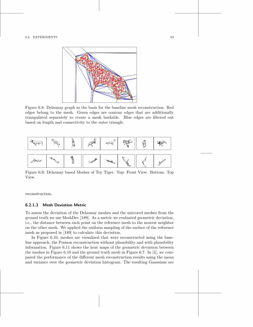
6.2. EXPERIMENTS 93
Figure 6.8: Delaunay graph as the basis for the baseline mesh reconstruction. Rededges belong to the mesh. Green edges are contour edges that are additionallytriangulated separately to create a mesh backside. Blue edges are filtered outbased on length and connectivity to the outer triangle.
Figure 6.9: Delaunay based Meshes of Toy Tiger. Top: Front View. Bottom: TopView.
reconstruction.
6.2.1.3 Mesh Deviation Metric
To assess the deviation of the Delaunay meshes and the mirrored meshes from theground truth we use MeshDev [189]. As a metric we evaluated geometric deviation,i.e., the distance between each point on the reference mesh to the nearest neighboron the other mesh. We applied the uniform sampling of the surface of the referencemesh as proposed in [189] to calculate this deviation.
In Figure 6.10, meshes are visualized that were reconstructed using the base-line approach, the Poisson reconstruction without plausibility and with plausibilityinformation. Figure 6.11 shows the heat maps of the geometric deviation betweenthe meshes in Figure 6.10 and the ground truth mesh in Figure 6.7. In [4], we com-pared the performance of the different mesh reconstruction results using the meanand variance over the geometric deviation histogram. The resulting Gaussians are
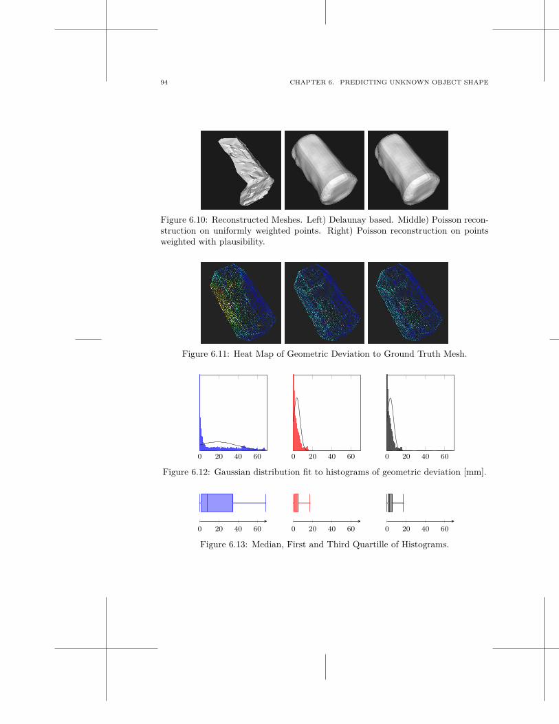
94 CHAPTER 6. PREDICTING UNKNOWN OBJECT SHAPE
Figure 6.10: Reconstructed Meshes. Left) Delaunay based. Middle) Poisson recon-struction on uniformly weighted points. Right) Poisson reconstruction on pointsweighted with plausibility.
Figure 6.11: Heat Map of Geometric Deviation to Ground Truth Mesh.
0 20 40 60 0 20 40 60 0 20 40 60
Figure 6.12: Gaussian distribution fit to histograms of geometric deviation [mm].
0 20 40 60 0 20 40 60 0 20 40 60
Figure 6.13: Median, First and Third Quartille of Histograms.
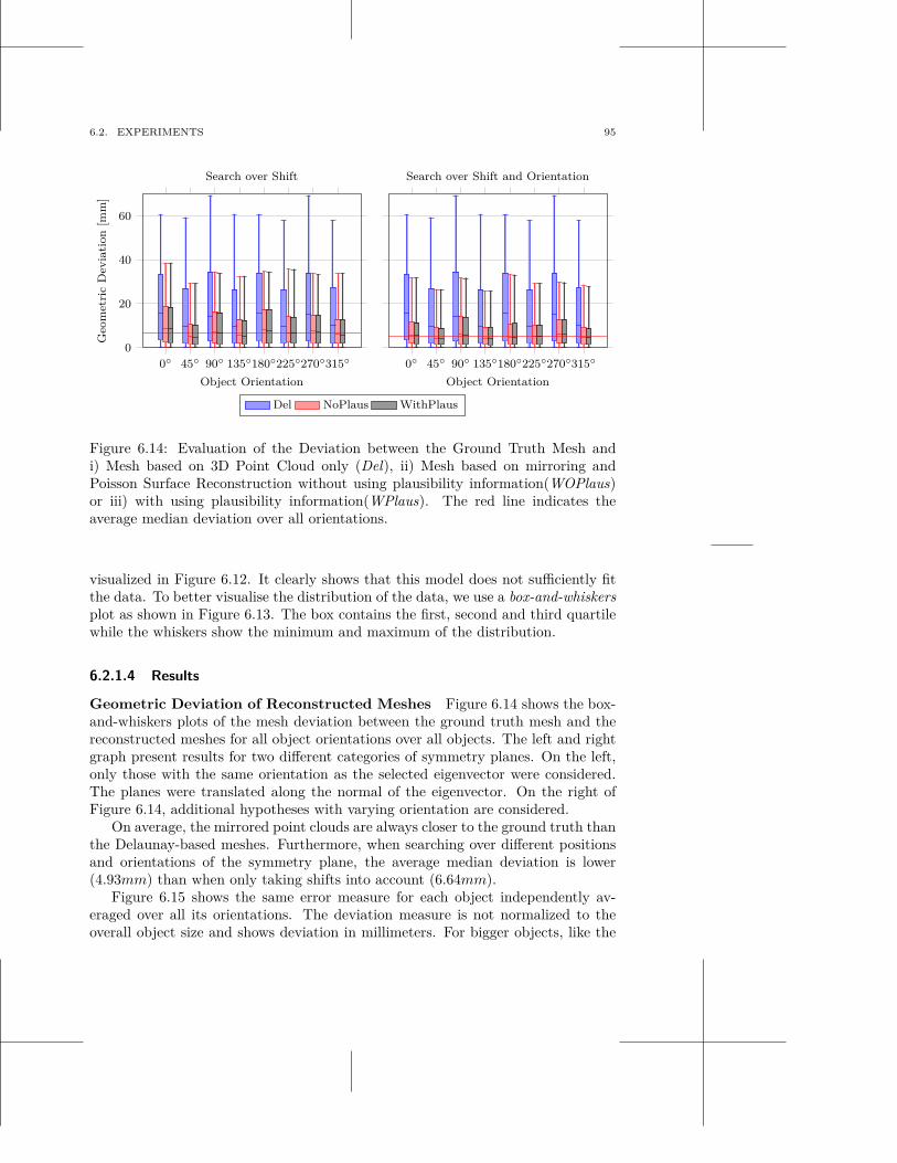
6.2. EXPERIMENTS 95
0◦ 45◦ 90◦ 135◦180◦225◦270◦315◦
0
20
40
60
Object Orientation
Geo
met
ric
Dev
iati
on
[mm
]
Search over Shift
0◦ 45◦ 90◦ 135◦180◦225◦270◦315◦
Object Orientation
Search over Shift and Orientation
Del NoPlaus WithPlaus
Figure 6.14: Evaluation of the Deviation between the Ground Truth Mesh andi) Mesh based on 3D Point Cloud only (Del), ii) Mesh based on mirroring andPoisson Surface Reconstruction without using plausibility information(WOPlaus)or iii) with using plausibility information(WPlaus). The red line indicates theaverage median deviation over all orientations.
visualized in Figure 6.12. It clearly shows that this model does not sufficiently fitthe data. To better visualise the distribution of the data, we use a box-and-whiskersplot as shown in Figure 6.13. The box contains the first, second and third quartilewhile the whiskers show the minimum and maximum of the distribution.
6.2.1.4 Results
Geometric Deviation of Reconstructed Meshes Figure 6.14 shows the box-and-whiskers plots of the mesh deviation between the ground truth mesh and thereconstructed meshes for all object orientations over all objects. The left and rightgraph present results for two different categories of symmetry planes. On the left,only those with the same orientation as the selected eigenvector were considered.The planes were translated along the normal of the eigenvector. On the right ofFigure 6.14, additional hypotheses with varying orientation are considered.
On average, the mirrored point clouds are always closer to the ground truth thanthe Delaunay-based meshes. Furthermore, when searching over different positionsand orientations of the symmetry plane, the average median deviation is lower(4.93mm) than when only taking shifts into account (6.64mm).
Figure 6.15 shows the same error measure for each object independently av-eraged over all its orientations. The deviation measure is not normalized to theoverall object size and shows deviation in millimeters. For bigger objects, like the
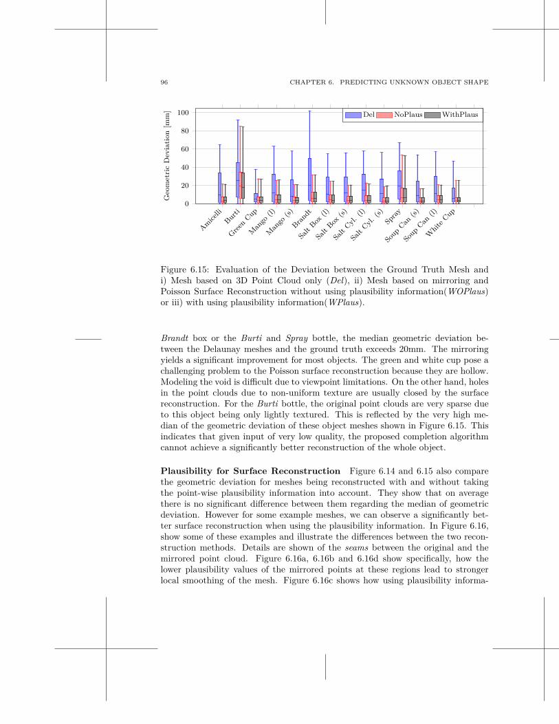
96 CHAPTER 6. PREDICTING UNKNOWN OBJECT SHAPE
Am
icelli
Bur
ti
Gre
enCup
Man
go(l)
Man
go(s
)
Bra
ndt
Salt
Box
(l)
Salt
Box
(s)
Salt
Cyl
.(l)
Salt
Cyl
.(s
)
Spra
y
Soup
Can
(s)
Soup
Can
(l)
Whi
teCup
0
20
40
60
80
100
Geo
met
ric
Dev
iati
on
[mm
]
Del NoPlaus WithPlaus
Figure 6.15: Evaluation of the Deviation between the Ground Truth Mesh andi) Mesh based on 3D Point Cloud only (Del), ii) Mesh based on mirroring andPoisson Surface Reconstruction without using plausibility information(WOPlaus)or iii) with using plausibility information(WPlaus).
Brandt box or the Burti and Spray bottle, the median geometric deviation be-tween the Delaunay meshes and the ground truth exceeds 20mm. The mirroringyields a significant improvement for most objects. The green and white cup pose achallenging problem to the Poisson surface reconstruction because they are hollow.Modeling the void is difficult due to viewpoint limitations. On the other hand, holesin the point clouds due to non-uniform texture are usually closed by the surfacereconstruction. For the Burti bottle, the original point clouds are very sparse dueto this object being only lightly textured. This is reflected by the very high me-dian of the geometric deviation of these object meshes shown in Figure 6.15. Thisindicates that given input of very low quality, the proposed completion algorithmcannot achieve a significantly better reconstruction of the whole object.
Plausibility for Surface Reconstruction Figure 6.14 and 6.15 also comparethe geometric deviation for meshes being reconstructed with and without takingthe point-wise plausibility information into account. They show that on averagethere is no significant difference between them regarding the median of geometricdeviation. However for some example meshes, we can observe a significantly bet-ter surface reconstruction when using the plausibility information. In Figure 6.16,show some of these examples and illustrate the differences between the two recon-struction methods. Details are shown of the seams between the original and themirrored point cloud. Figure 6.16a, 6.16b and 6.16d show specifically, how thelower plausibility values of the mirrored points at these regions lead to strongerlocal smoothing of the mesh. Figure 6.16c shows how using plausibility informa-
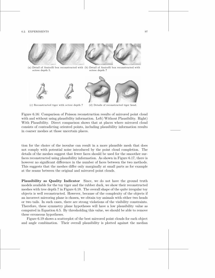
6.2. EXPERIMENTS 97
(a) Detail of Amicelli box reconstructed withoctree depth 5.
(b) Detail of Amicelli box reconstructed withoctree depth 7
(c) Reconstructed tiger with octree depth 7 (d) Details of reconstructed tiger head.
Figure 6.16: Comparison of Poisson reconstruction results of mirrored point cloudwith and without using plausibility information. Left) Without Plausibility. Right)With Plausibility. Direct comparison shows that at places where mirrored cloudconsists of contradicting oriented points, including plausibility information resultsin coarser meshes at those uncertain places.
tion for the choice of the isovalue can result in a more plausible mesh that doesnot comply with potential noise introduced by the point cloud completion. Thedetails of the meshes suggest that fewer faces should be used for the smoother sur-faces reconstructed using plausibility information. As shown in Figure 6.17, there ishowever no significant difference in the number of faces between the two methods.This suggests that the meshes differ only marginally at small parts as for exampleat the seams between the original and mirrored point clouds.
Plausibility as Quality Indicator Since, we do not have the ground truthmodels available for the toy tiger and the rubber duck, we show their reconstructedmeshes with tree depth 7 in Figure 6.18. The overall shape of the quite irregular toyobjects is well reconstructed. However, because of the complexity of the objects ifan incorrect mirroring plane is chosen, we obtain toy animals with either two headsor two tails. In such cases, there are strong violations of the visibility constraints.Therefore, these symmetry plane hypotheses will have a low plausibility value ascomputed in Equation 6.5. By thresholding this value, we should be able to removethese erroneous hypotheses.
Figure 6.19 shows a scatterplot of the best mirrored point clouds for each objectand angle combination. Their overall plausibility is plotted against the median
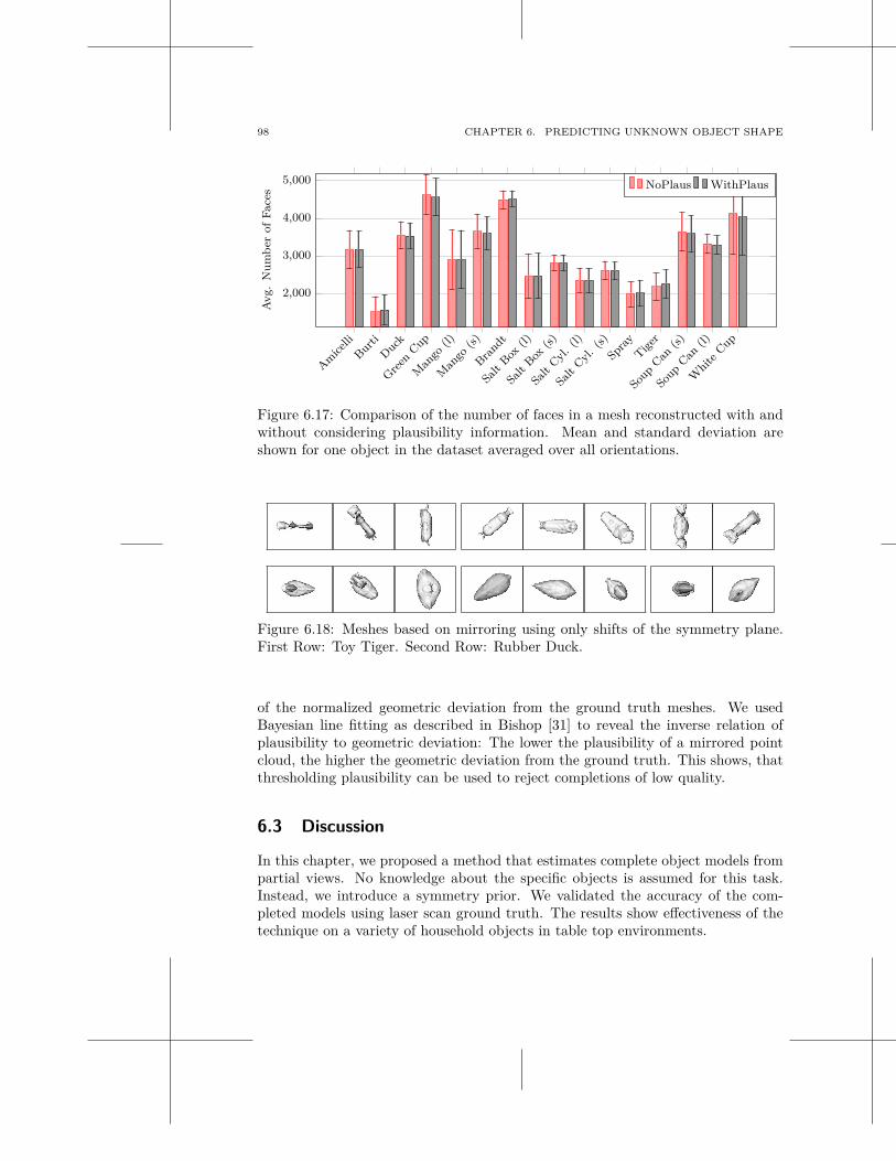
98 CHAPTER 6. PREDICTING UNKNOWN OBJECT SHAPE
Am
icelli
Bur
ti
Duc
k
Gre
enCup
Man
go(l)
Man
go(s
)
Bra
ndt
Salt
Box
(l)
Salt
Box
(s)
Salt
Cyl
.(l)
Salt
Cyl
.(s
)
Spra
y
Tig
er
Soup
Can
(s)
Soup
Can
(l)
Whi
teCup
2,000
3,000
4,000
5,000
Av
g.
Nu
mb
erof
Face
s
NoPlaus WithPlaus
Figure 6.17: Comparison of the number of faces in a mesh reconstructed with andwithout considering plausibility information. Mean and standard deviation areshown for one object in the dataset averaged over all orientations.
Figure 6.18: Meshes based on mirroring using only shifts of the symmetry plane.First Row: Toy Tiger. Second Row: Rubber Duck.
of the normalized geometric deviation from the ground truth meshes. We usedBayesian line fitting as described in Bishop [31] to reveal the inverse relation ofplausibility to geometric deviation: The lower the plausibility of a mirrored pointcloud, the higher the geometric deviation from the ground truth. This shows, thatthresholding plausibility can be used to reject completions of low quality.
6.3 Discussion
In this chapter, we proposed a method that estimates complete object models frompartial views. No knowledge about the specific objects is assumed for this task.Instead, we introduce a symmetry prior. We validated the accuracy of the com-pleted models using laser scan ground truth. The results show effectiveness of thetechnique on a variety of household objects in table top environments.
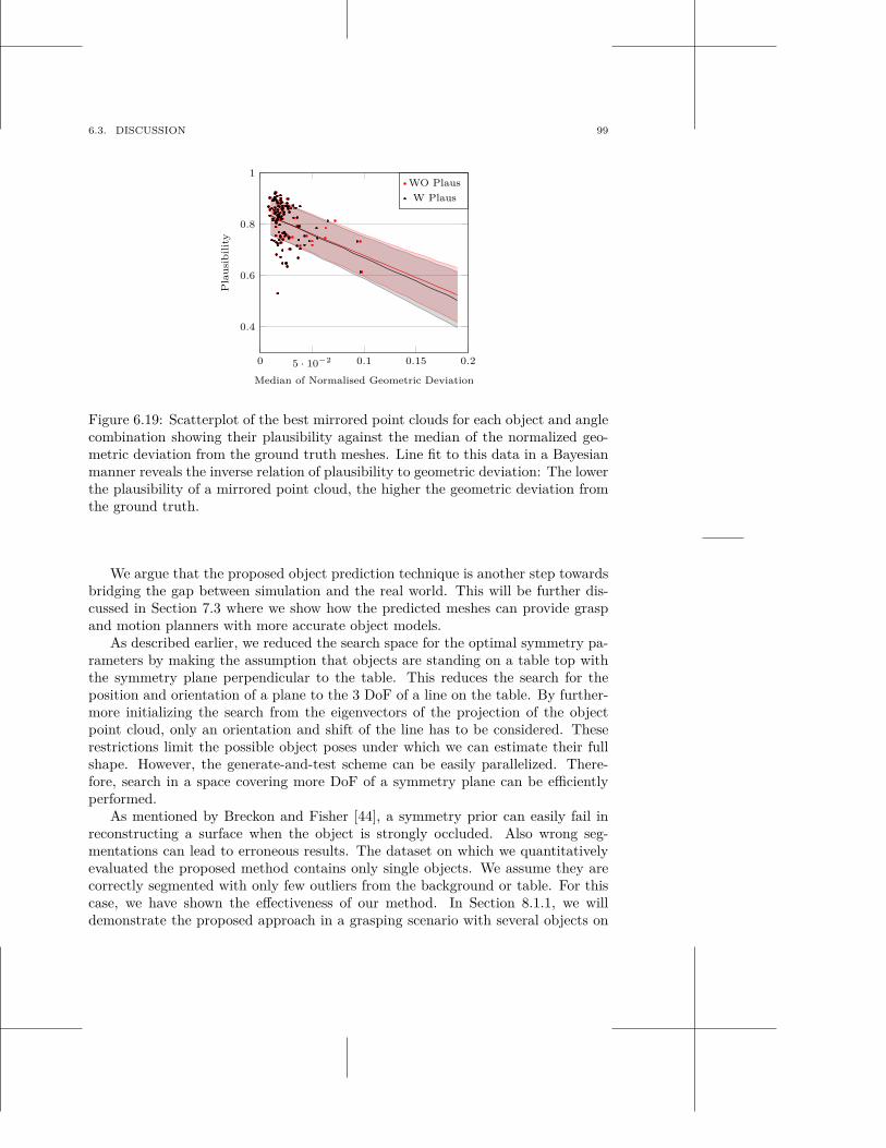
6.3. DISCUSSION 99
0 5 · 10−2 0.1 0.15 0.2
0.4
0.6
0.8
1
Median of Normalised Geometric Deviation
Pla
usi
bil
ity
WO Plaus
W Plaus
Figure 6.19: Scatterplot of the best mirrored point clouds for each object and anglecombination showing their plausibility against the median of the normalized geo-metric deviation from the ground truth meshes. Line fit to this data in a Bayesianmanner reveals the inverse relation of plausibility to geometric deviation: The lowerthe plausibility of a mirrored point cloud, the higher the geometric deviation fromthe ground truth.
We argue that the proposed object prediction technique is another step towardsbridging the gap between simulation and the real world. This will be further dis-cussed in Section 7.3 where we show how the predicted meshes can provide graspand motion planners with more accurate object models.
As described earlier, we reduced the search space for the optimal symmetry pa-rameters by making the assumption that objects are standing on a table top withthe symmetry plane perpendicular to the table. This reduces the search for theposition and orientation of a plane to the 3 DoF of a line on the table. By further-more initializing the search from the eigenvectors of the projection of the objectpoint cloud, only an orientation and shift of the line has to be considered. Theserestrictions limit the possible object poses under which we can estimate their fullshape. However, the generate-and-test scheme can be easily parallelized. There-fore, search in a space covering more DoF of a symmetry plane can be efficientlyperformed.
As mentioned by Breckon and Fisher [44], a symmetry prior can easily fail inreconstructing a surface when the object is strongly occluded. Also wrong seg-mentations can lead to erroneous results. The dataset on which we quantitativelyevaluated the proposed method contains only single objects. We assume they arecorrectly segmented with only few outliers from the background or table. For thiscase, we have shown the effectiveness of our method. In Section 8.1.1, we willdemonstrate the proposed approach in a grasping scenario with several objects on
100 CHAPTER 6. PREDICTING UNKNOWN OBJECT SHAPE
a table top. Although minor occlusions occur, the method still succeeds in providingmodels on which successful grasps are planned and finally executed.
However, in the presence of strong occlusions the proposed method will mostlikely fail to estimate the correct object surface. Among others, this is due to usingthe eigenvectors of the point cloud projection as an initialization for the underlyingsymmetry plane. This choice has been shown on the dataset to yield reasonableestimates for the orientation of the symmetry plane. However, if the point cloudrepresents only a minor part of the real object, then the eigenvector of this partwill not be close to the optimal symmetry plane of the real object.
We see two possibilities to overcome this limitation. The first one is based onusing plausibility of a symmetry plane hypothesis as an absolute quality indicator.That this is possible has been shown earlier in this chapter. If only a hypothesiscan be found that strongly violates visibility constraints, i.e., has a low plausibility,it can be rejected completely by thresholding this value. Then, a different methodfor motion and grasp planning has to be used.
A second possibility is to keep the predicted object shape but explicitly takethe uncertainty about the reconstructed surface into account for grasp and motionplanning. This could be done by for example avoiding placements of the hand inwhich fingertip positions coincide with points of low plausibility. Another optionis to use the proposed method in combination with haptic exploration such thatespecially uncertain parts of the estimated object surface are confirmed with thehand first.

7
Generation of Grasp Hypotheses
Autonomous grasping of objects in unstructured environments remains an openproblem in the robotics community. Even if the robot achieves a good under-standing of the scene with well-segmented objects, the decision on how to grasp ormanipulate them depends on many factors, e.g., the identity and geometry of theobject, the scene context, the embodiment of the robot or its task. The number ofpotentially applicable grasps to a single object is immense. In the following, we willrefer to this set as grasp candidates. Two main challenges exist: (i) planning goodgrasps. This can be seen as choosing a set of promising grasp hypotheses among thecandidates. And (ii) executing these robustly under uncertainties introduced bythe perception or motor system. In Chapter 8, different approaches towards robustgrasp execution will be discussed. In this chapter, we will propose approaches togenerate good grasp hypotheses given different prior object knowledge. In our case,one hypothesis is defined by
• the grasping point on the object with which the tool centre point (TCP) shouldbe aligned 1,
• the approach vector [70] which describes the 3D angle that the robot handapproaches the grasping point with and
• the wrist orientation of the robotic hand.
Although humans master grasping easily, no suitable representations of thewhole process have yet been proposed in the neuro-scientific literature, makingit difficult to develop robotic systems that can mimic human grasping behavior.However, there is some valuable insight. Goodale [91] proposes that the humanvisual system is characterized by a division into the dorsal and ventral pathway.While the dorsal stream is mainly responsible for the spatial vision targeted atextracting action-relevant visual features, the ventral stream is engaged in the taskof object identification. This dissociation also suggests two different grasp choicemechanisms dependent on whether a known or unknown object is to be manipu-lated. Support for this can be found in behavioral studies by Borghi [38] and Creem
1In this thesis, the TCP is at the centre of palm of the robotic gripper.
101
102 CHAPTER 7. GENERATION OF GRASP HYPOTHESES
and Proffitt [57]. The authors claim that in the case of novel objects, our actionsare purely guided by affordances as introduced by Gibson [89]. In the case of knownobjects, semantic information (e.g., through grasp experience) is needed to graspthem appropriately according to their function. However as argued in [91, 48, 228]this division of labour is not absolute. In the case of objects that are similar to pre-viously encountered ones, the ventral system helps the dorsal stream in the actionselection process by providing information about prehensile parts along with theirafforded actions.
Grasp synthesis algorithms have previously been reviewed by Sahbani et al.[198]. The authors divide the approaches into analytical and empirical methods.With analytic, they refer to all those methods that find optimal grasps according tosome criteria. This can be based on geometric, kinematic or dynamic formulationsas for example force or form closure. Empirical approaches on the other hand avoidcomputing these mathematical or physical models. Instead, a set of example graspsis sampled from the set of candidates, their quality evaluated and the best subsetis chosen as the final grasp hypotheses. Kamon et al. [108] also refer to this as thecomparative approach. Existing algorithms differ in the source of grasp candidatesand the definition of their quality.
In [198] the division is made dependent on whether the method is based onobject features or observation of humans during grasping. We believe that thisfalls short of capturing the diversity of the empirical approaches. In this thesis,we instead group existing empirical grasp synthesis algorithms according to theassumed prior knowledge about object hypotheses. The three categories are:
• Known Objects: These approaches consider grasping of a-priori known ob-jects. Once the object is identified, the goal is to estimate its pose and retrievea suitable grasp, e.g., from an experience database.
• Unknown Objects: Approaches that fall into this category commonly representthe shape of an unknown object and apply heuristics to reduce the numberof potential grasps.
• Familiar Objects: These approaches try to transfer pre-existing grasp expe-rience from similar objects. Objects can be familiar on different levels. Lowlevel similarity can for example be defined in terms of shape, color or texture.Higher level similarity could be defined based on object category. A underly-ing assumption is that new objects similar to the old ones can be grasped ina similar way.
This kind of division is inspired by the research in the field of neuropsychol-ogy. It is suitable because the assumed prior object knowledge determines thenecessary perceptual processing but also what empirical method can be used forgenerating grasp candidates. This will be discussed in more detail in Section 7.1.Following related work, we will propose different grasp inference methods for eitherknown, familiar or unknown objects. Our requirements on the employed object
7.1. RELATED WORK 103
representations are that they have to be rich enough to allow for the inference ofthe aforementioned grasp parameters.
7.1 Related Work
Figure 7.1 outlines the different aspects that influence the generation of grasp hy-potheses for an object. In this section, we focus on the significant body of workproposing empirical grasp synthesis methods. For an in-depth review of analyti-cal approaches, we refer to [198]. We use the division proposed in the previoussection to review the related work. Given the kind of prior object knowledge, wewill discuss the different object representations that are partially dependent on thekind of sensor the robot is equipped with. Furthermore, we are also interested inwhich empirical method is employed as outlined in Figure 7.2. There is a number ofmethods that learn either from humans, labeled examples or trial and error. Othermethods use heuristics to prune the search space for appropriate grasp hypotheses.
There is relatively little work on task-dependent grasping. Also, embodiment isusually not in the focus of the approaches discussed here. These two aspects willtherefore be mentioned but not discussed in depth.
7.1.1 Grasping Known Objects
If the robot knows the object that it has to grasp, then the problem of finding agood grasp reduces to the online estimation of the object’s pose. Given this, a setof grasp hypotheses can be retrieved from an experience database and filtered byreachability.
7.1.1.1 Offline Generation of a Grasp Experience Database
In this section, we will look at approaches that set up an experience database. Theydiffer in how candidate grasps are generated and in how their quality is evaluated.These two aspects are usually tightly connected and also depend on the objectrepresentation.
3D Mesh Models and Contact-Level Grasping The main problem in thearea of grasp synthesis is the huge search space from which a good grasp has to beretrieved. Its size is due to the large number of hand configurations that can beapplied to a given object. In the theory of contact-level grasping [161, 204] a goodgrasp is defined from the perspective of forces, friction and wrenches. Based onthis, different criteria are defined to rate grasp configurations, e.g., force closure,dexterity, equilibrium, stability and dynamic behavior.
Several approaches in the area of grasp synthesis exist that apply these criteriato rank grasp candidates for an object with a given 3D mesh model. They differ inthe heuristics they use to generate the candidates. Some of them approximate theobject’s shape with a constellation of primitives such as spheres, cones, cylinders and
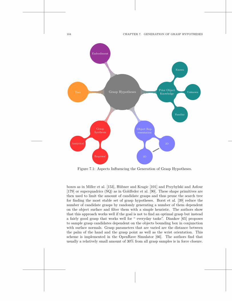
104 CHAPTER 7. GENERATION OF GRASP HYPOTHESES
Grasp Hypotheses Prior ObjectKnowledge
Known
Unknown
Familiar
Object Rep-resentation
2D
3D
GraspSynthesis
Analytical
Empirical
Task
Embodiment
Figure 7.1: Aspects Influencing the Generation of Grasp Hypotheses.
boxes as in Miller et al. [153], Hübner and Kragic [101] and Przybylski and Asfour[179] or superquadrics (SQ) as in Goldfeder et al. [90]. These shape primitives arethen used to limit the amount of candidate grasps and thus prune the search treefor finding the most stable set of grasp hypotheses. Borst et al. [39] reduce thenumber of candidate grasps by randomly generating a number of them dependenton the object surface and filter them with a simple heuristic. The authors showthat this approach works well if the goal is not to find an optimal grasp but insteada fairly good grasp that works well for “ everyday tasks”. Diankov [65] proposesto sample grasp candidates dependent on the objects bounding box in conjunctionwith surface normals. Grasp parameters that are varied are the distance betweenthe palm of the hand and the grasp point as well as the wrist orientation. Thisscheme is implemented in the OpenRave Simulator [66]. The authors find thatusually a relatively small amount of 30% from all grasp samples is in force closure.
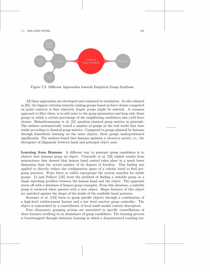
7.1. RELATED WORK 105
EmpiricalGrasp Synthesis
HeuristicsLearning
HumanDemon-stration
LabeledTraining
Data
Trial &Error
Figure 7.2: Different Approaches towards Empirical Grasp Synthesis.
All these approaches are developed and evaluated in simulation. As also claimedin [65], the biggest criticism towards ranking grasps based on force closure computedon point contacts is that relatively fragile grasps might be selected. A commonapproach to filter these, is to add noise to the grasp parameters and keep only thosegrasps in which a certain percentage of the neighboring candidates also yield forceclosure. Balasubramanian et al. [21] question classical grasp metrics in principle.The authors systematically tested a number of grasps in the real world that werestable according to classical grasp metrics. Compared to grasps planned by humansthrough kinesthetic learning on the same objects, these grasps underperformedsignificantly. The authors found that humans optimise a skewness metric, i.e., thedivergence of alignment between hand and principal object axes.
Learning from Humans A different way to generate grasp candidates is toobserve how humans grasp an object. Ciorcarlie et al. [53] exploit results fromneuroscience that showed that human hand control takes place in a much lowerdimension than the actual number of its degrees of freedom. This finding wasapplied to directly reduce the configuration space of a robotic hand to find pre-grasp postures. From these so called eigengrasps the system searches for stablegrasps. Li and Pollard [135] treat the problem of finding a suitable grasp as ashape matching problem between the human hand and the object. The approachstarts off with a database of human grasp examples. From this database, a suitablegrasp is retrieved when queried with a new object. Shape features of this objectare matched against the shape of the inside of the available hand postures.
Kroemer et al. [124] learn to grasp specific objects through a combination ofa high-level reinforcement learner and a low level reactive grasp controller. Theobject is represented by a constellation of local multi-modal contour descriptors.
Four elementary grasping actions are associated to specific constellations ofthese features resulting in an abundance of grasp candidates. The learning processis bootstrapped through imitation learning in which a demonstrated reaching tra-
106 CHAPTER 7. GENERATION OF GRASP HYPOTHESES
jectory recorded with a VICON system is converted into an initial policy. Similarinitialization of an object specific grasping policy is used in Pastor et al. [167] andStulp et al. [214] through kinesthetic learning. Detry et al. [62, 64] use the samesparse object model as Kroemer et al. [124]. The set of associated grasp hypothe-ses is modelled as a non-parametric density functions in the space of 6D gripperposes, referred to as a bootstrap density. In [62] human grasp examples are used tobuild an object specific empirical grasp density from which grasp hypotheses canbe sampled.
Faria et al. [76] use a multi-modal data acquisition tool to record humans grasp-ing specific objects. Objects are represented as probabilistic volumetric maps thatintegrate multi-modal information such as contact regions, fixation points and tac-tile forces. This information is then used to annotate object parts as graspable ornot. However, no results are provided on how a robot can transfer this informationto new objects and to its own embodiment. Romero et al. [186] present a systemfor observing humans visually while they interact with an object. A grasp type andpose is recognized and mapped to different robotic hands in a fixed scheme. Forvalidation of the approach in the simulator, 3D object models are used. Examplesof real-world executions are shown. The object is not explicitly modelled. Instead,it is assumed that human and robot act on the same object in the same pose.
Learning through Self-Experience Instead of adopting a fixed set of graspcandidates given for example by a person, the following approaches try to refinethem by trial and error. In [124, 214] reinforcement learning is used to improvean initial human demonstration. Kroemer et al. [124] uses a low-level reactivecontroller to perform the grasp that informs the high level controller with rewardinformation. Stulp et al. [214] increase the robustness of their non-reactive graspingstrategy by learning shape and goal parameters of the motion primitives that areused to model a full grasping action. Through this approach, the robot learns reach-ing trajectories and grasps that are robust against object pose uncertainties. AlsoDetry et al. [64], adopt an approach in which the robot learns to grasp specific ob-jects by experience. Instead of human examples as in [62], successful grasping trialsare used to build the object-specific empirical grasp density. This non-parametricdensity can then be used to sample grasp hypotheses.
7.1.1.2 Online Object Pose Estimation
In the previous section, we reviewed different approaches towards grasping knownobjects regarding their way to generate candidate grasps and rank them to forma set of grasp hypotheses. During online execution, an object has to be first rec-ognized and its pose estimated before the offline trained grasps can be executed.Furthermore, from the set of hypotheses not all grasps might be applicable in thecurrent scenario. An appropriate selection has to be made.
Several of the aforementioned grasp generation methods [124, 62, 64] use theprobabilistic approach towards object representation and pose estimation proposed
7.1. RELATED WORK 107
by Detry et al. [63]. As described before, grasps are either selected by samplingfrom densities [62, 64] or a grasp policy refined from a human demonstration isapplied [124].
The following approaches use offline generated experience databases throughsimulation of grasps on 3D models in either GraspIt! [152] or OpenRave [66]. Beren-son et al. [27] consider this experience database then as one factor in selecting anappropriate grasp. The second factor in computing the final grasp score is the wholescene geometry. The approach was demonstrated on a real robot using a motioncapture system to determine the robot and the object position.
In the online stage of the method presented by Ekvall and Kragic [70], a humandemonstrator wearing a magnetic tracking device is observed while manipulating aspecific object. The grasp type is recognized and mapped through a fixed schemato a set of robotic hands. Given the grasp type and the hand, the best approachvector is selected from an offline trained experience database. Unlike Detry et al.[62] and Romero et al. [186], the approach vector used by the demonstrator is notadopted. Ekvall and Kragic [70] assume that the object pose is known. However,experiments are conducted in which pose error is simulated. No demonstrationon a real robot is shown. Morales et al. [156] use the method proposed by Azadet al. [19] to recognize an object and estimate its pose from a monocular image.Given that information, an appropriate grasp configuration can be selected froma grasp experience database that has been acquired offline. The whole system isdemonstrated on the robotic platform described in Asfour et al. [16]. Huebner et al.[102] demonstrate grasping of known objects on the same humanoid platform andthe same method for object recognition and pose estimation. The offline selectionof grasp hypotheses is based on a decomposition into boxes. Ciocarlie et al. [52]propose a robust grasping pipeline in which known object models are fitted to pointcloud clusters using standard ICP [30]. Knowledge about the table plane and theassumption that objects are rotationally symmetric and are always standing uprighthelps in reducing the search space of potential object poses.
All of the aforementioned methods assume prior knowledge on a rigid 3D objectmodel. Jared Glover [107] consider known deformable objects. For representingthem, probabilistic models of their 2D shape are learnt. The objects can thenbe detected in monocular images of cluttered scenes even when they are partiallyoccluded. The visible object parts serve as a basis for planning a stable grasp underconsideration of the global object shape. Collet Romea et al. [55] use a combinationof 2D and 3D features as an object model. The authors estimate the object’s posein a scene from a single image. The accuracy of their approach is demonstratedthrough a number of successful grasps on 4 different objects in somewhat clutteredscenes. Other robust methods for estimating the pose of single or multiple objectssimultaneously are presented in [95, 68, 165, 166]. Although these approaches aremotivated in a grasping scenario, no actual grasping has been shown.
108 CHAPTER 7. GENERATION OF GRASP HYPOTHESES
7.1.1.3 Learning Object Models
All of the above mentioned approaches are dependent on an a-priori known denseor detailed object model either in 2D or in 3D that may be difficult to obtain.
Different methods have been proposed to build a model of a new object bycombining a sequence of observations. Foix et al. [81] present a method for mergingpartial object point clouds when facing strong noise in the data and uncertaintyin the estimated camera trajectory. The approach is based on standard ICP forregistering point clouds of two consecutive views. The uncertainty in the resultingcamera pose estimates is estimated by propagating the sensor covariance throughthe ICP minimization. Collet Romea et al. [55] proposes to acquire object modelsoffline consisting of an image, a sparse 3D model and a simplified mesh model.A method towards autonomous learning of object surface models is demonstratedby Krainin et al. [123]. The robot holds an object in its hand and plans the nextbest views to acquire a surface mesh. An alternative way to learn object modelsis taken by Tenorth et al. [218]. Here, web-enabled robots are proposed that canretrieve appearance and 3D models from online databases.
7.1.2 Grasping Unknown Objects
If the currently considered object hypothesis could not be recognized as a knownobject and is not similar to one either, then it is considered as unknown. In thiscase, the previously listed approaches are not applicable since in practice it is verydifficult to infer object geometry fully and accurately from measurements takenfrom sensor devices such as cameras and laser range finders. There are various waysto deal with this sparse, incomplete and noisy data. We divided the approachesroughly into methods that try to approximate the shape of an object, methods thatgenerate grasps based on low-level features and a set of heuristics and methods thatrely mostly on the global shape of the object hypothesis.
7.1.2.1 Approximating Unknown Object Shape
One approach towards generating grasp hypotheses for unknown objects is to ap-proximate them with shape primitives that provide cues for potential grasps. Duneset al. [67] approximate the rough object shape with a quadric whose minor axis isused to infer the wrist orientation. The object centroid serves as the approach tar-get and the rough object size helps to determine the hand pre-shape. The quadricis estimated from multi-view measurements of object shape in monocular images.Opposed to the above mentioned techniques, Bone et al. [37] make no prior as-sumption about the shape of the object. They apply shape carving for the purposeof grasping with a parallel-jaw gripper. After obtaining a model of the object, theysearch for a pair of reasonably flat and parallel surfaces that are best suited for thiskind of manipulator.
7.1. RELATED WORK 109
7.1.2.2 From Low-Level Features to Grasp Hypotheses
A common approach is to map low-level features to an abundance of grasp hy-potheses and then rank them dependent on a set criteria. Kraft et al. [120] usea stereo camera to extract a representation of the scene. Instead of a raw pointcloud, they are processing it further to obtain a sparser model consisting of localmulti-modal contour descriptors already mentioned above in conjunction with thework by Detry et al. [62, 64] and Kroemer et al. [124]. Four elementary graspingactions are associated to specific constellations of these features. With the helpof heuristics the huge number of resulting grasp hypothesis is reduced. Popovićet al. [172] present an extension of this system that also uses local surfaces andtheir interrelations to propose and filter two and three-fingered grasp hypotheses.The feasibility of the approach is evaluated in a mixed real-world and simulatedenvironment.
Hsiao et al. [99] employ several heuristics for generating grasp hypotheses de-pendent on the shape of the segmented point cloud. These can be grasps from thetop, from the side or applied to high points of the objects. The generated hypothe-ses are then ranked using a weighted list of features such as for example numberof points within the gripper, distance between the fingertip and the center of thesegment or whether the object fits into the whole hand. This method is integratedinto the grasping pipeline proposed in [52] for the segmented point cloud clustersthat did not get recognized as a specific object.
The main idea presented by Klingbeil et al. [118] is to search for a pattern inthe scene that is similar to the 2D cross section of the robotic gripper interior. Adepth image serves as the input to the method and is sampled to find a set of grasphypotheses. These are ranked according to an objective functions that takes pairsof these grasp hypotheses and their local structure into account.
7.1.2.3 From Global Shape to Grasp Hypothesis
Other approaches use the global shape of an object to infer one good grasp hypoth-esis. Richtsfeld and Vincze [184] use a segmented point cloud from a stereo camera.They are searching for a suitable grasp with a simple gripper based on the shift ofthe top plane of an object into its centre of mass. A set of heuristics is used forselecting promising fingertip positions. Maldonado et al. [142] model the object asa 3D Gaussian. For choosing a grasp configuration, it optimises a criterion in whichthe distance between palm and object is minimised while the distance between fin-gertips and the object is maximised. Stückler et al. [213] generate grasp hypothesesbased on eigenvectors of the object’s footprints on the table. With footprints, werefer to the 3D object point cloud projected onto the supporting surface. A similarapproach has been taken in our previous work [10]. This approach is related to[21] in which it is shown that people are optimizing the aforementioned skewnessmeasure.
110 CHAPTER 7. GENERATION OF GRASP HYPOTHESES
7.1.2.4 Assuming Symmetry
Many of the man-made objects surrounding us possess one or more symmetries.Exploiting this, allows us to predict unobserved parts of an object hypothesis.Marton et al. [147] show how grasp selection can be performed based on such anapproximation of unobserved object shape. Using footprint analysis, objects witha box and a cylinder shape are reconstructed. The remaining object hypothesesare analysed in terms of more complex rotational symmetry and reconstructedby fitting a curve to a cross section of the point cloud. For grasp planning, thereconstructed object is imported to a simulator. Grasp candidates are generatedthrough randomisation of grasp parameters on which then the force-closure criteriais evaluated. Rao et al. [180] sample grasp points from the surface of a segmentedobject. The normal of the local surface at this point serves as a search directionfor a second contact point. This is chosen to be at the intersection between theextended normal and the opposite side of the object. By assuming symmetry, thissecond contact point is assumed to have a contact normal in the direction oppositeto the normal of the first contact point.
In Chapter 6, we presented a related approach that does not rely on selecting thekind of symmetry prior to reconstruction. Furthermore, it takes the complete pointcloud for reconstruction into account and not only a local patch. In Section 7.3,different methods to generate grasp candidate on the resulting completed objectmodels are presented.
7.1.3 Grasping Familiar Objects
A promising direction in the area of grasp planning is to re-use experience to graspfamiliar objects. Many of the objects surrounding us can be grouped together intocategories of common characteristics. There are different possibilities what thesecommonalities can be. In the computer vision community, objects within one cat-egory usually share characteristic visual properties. These can be, e.g., a commontexture [205] or shape [79, 26], the occurrence of specific local features [60, 127] ortheir specific spatial constellation [133, 131]. These categories are usually referredto as basic level categories and emerged from the area of cognitive psychology [187].
In robotics however, and specifically in the area of manipulation, the goal is toenable an embodied, cognitive agent to interact with these objects. In this case,objects in one category should share common affordances [211]. More specifically,this means that they should also be graspable in a similar way. The difficulty then isto find a representation that can encode this common affordance and is grounded inthe embodiment and cognitive capabilities of the agent. Given this representation,a similarity metric has to be found under which different objects can be comparedto each other.
The following approaches try to learn from experience how objects can begrasped. This is different from the aforementioned systems in which objects areassumed to be unknown, i.e, dissimilar to any object encountered previously. There
7.1. RELATED WORK 111
the difficulty lies in finding appropriate rules and heuristics. In the following, we willpresent related work that tackles the grasping of familiar objects and specificallyfocus on the applied representations.
7.1.3.1 Based on 3D Data
First of all, there are approaches that rely on 3D data only. For example, El-Khouryand Sahbani [72] segment a given point cloud into parts and approximate each partby a SQ. An artificial neural network (ANN) is used to classify whether or not thepart is prehensile. The ANN has been trained beforehand on labeled SQs. If oneof the object parts is classified as prehensile, an n-fingered force-closure grasp iscomputed on this object part. Pelossof et al. [168] use a single SQ to find a suitablegrasp configuration for a Barrett hand consisting of the approach vector, wrist ori-entation and finger spread. An SVM is trained on data consisting of feature vectorscontaining the parameters of the SQ and of the grasp configuration. They were la-belled with a scalar estimating the grasp quality. When feeding the SVM only withthe shape parameters of the SQ, their algorithm searches efficiently through thegrasp configuration space for parameters that maximise the grasp quality. Curtisand Xiao [59] build upon a database of 3D objects annotated with the best graspsthat can be applied to them. To infer a good grasp for a new object, very basicshape features, e.g., the aspect ratio of the object’s bounding box, are extracted toclassify it as similar to an object in the database. The assumption made in thisapproach is that similarly shaped objects can be grasped in a similar way. Songet al. [209] learn a Bayesian Network from labeled training data to model the jointdistribution between different variables describing a grasp. These variables can beobject or action related (object size and class as well as grasp position and finalhand configuration); they can describe constraints or be the task label. Given thelearnt joint distribution, different information can be inferred as for example thetask after having observed the object and the action features.
All these approaches were performed and evaluated in simulation where thecentral assumption is that accurate and detailed 3D models are available in a knownpose. There are only very few approaches, that only use 3D data from real-worldsensors to infer suitable grasps. One of them has been presented by Hübner andKragic [101]. A point cloud from a stereo camera is decomposed into a constellationof boxes. The simple geometry of a box reduces the number of potential graspssignificantly. To decide which of the sides of the boxes provides a good grasp,an ANN is trained offline. The projection of the point cloud inside a box to itssides provides the input to the ANN. The training data consists of a set of theseprojections from different objects labeled with the grasp quality metrics. Theseare computed by the GraspIt! Simulator while performing the according grasps.Although, grasp selection is demonstrated on one objects, it remains unclear howwell the ANN can generalize from the synthetic training set to real-world data.
112 CHAPTER 7. GENERATION OF GRASP HYPOTHESES
3D Descriptors of Objects for Categorization Recently, we have seen anincreasing amount of new approaches towards pure 3D descriptors of objects forcategorization. Although, the following methods look promising, it has not benshown yet that they provide a suitable base for generalizing grasps over an objectcategory. Rusu et al. [197, 195] provide extensions of [194] for either recognizingor categorizing objects and estimating their pose relative to the viewpoint. Whilein [195] quantitative results on real data are presented, [197] uses simulated objectpoint clouds only. Wohlkinger and Vincze [231] use a combination of different shapedescriptors of partial object views to retrieve matching objects of a specific categoryfrom a large database. The retrieval problem is formulated as a nearest-neighborapproach. Robustness is achieved by exploiting intra class view similarities.
Although 3D descriptor of object hypotheses are used in Marton et al. [148] andMarton et al. [146], they are combined with 2D features to increase the robust-ness of detection. These approaches will therefore be discussed in more detail inSection 7.1.3.3 together with other methods integrating several sensor modalities.
7.1.3.2 Based on 2D Data
As mentioned previously, the assumption of having a detailed and accurate 3D ob-ject model available for learning to generalize grasps may not always be valid. Thisis particularly the case with real-world data gathered from sensors like laser-rangefinders, the kinect, stereo or time-of-flight cameras. However, there are experience-based approaches that avoid this difficulty by relying mainly on 2D data.
Kamon et al. [108] propose one of the first approaches towards generalizinggrasp experience to novel objects. The aim is to learn a function f : Q → G thatmaps object- and grasp-candidate-dependent quality parameters Q to a grade Gof the grasp. An object is represented by its 2D silhouette, its center of mass andmain axis. The grasp is represented by two parameters f1 and f2 from which incombination with the object features the fingertip positions can be computed. Theauthors found that the normals of the object surface at the contact points and thedistance of the line connecting the contact points to the object’s center of massare highly reliable quality features for predicting the grade of a grasp. Learning isbootstrapped by the offline generation of a knowledge database containing graspparameters along with their grade. This knowledge database is then updated whilethe robot collects experience by grasping new objects. The system is restricted toplanar grasps and visual processing of top-down views on objects. It is thereforequestionable how robust this approach is to more cluttered environments and strongpose variations of the object.
Saxena et al. [200] proposed a system that infers a point at where to grasp anobject directly as a function of its image. The authors apply machine learning totrain a grasping point model on labelled synthetic images of a number of differentobjects. The classification is based on a feature vector containing local appearancecues regarding color, texture and edges of an image patch in several scales andof its 24 neighboring patches in the lowest scale. The system was used success-
7.1. RELATED WORK 113
fully to pick up objects from a dishwasher after it has been specifically trained forthis scenario. However, if more complex goals are considered that require subse-quent actions, e.g., pouring something from one container into another, semanticknowledge about the object and about suitable grasps regarding their functionalitybecomes necessary [38, 57, 94]. Then, to only represent graspable points withoutthe conception of objectness [120][9] is not sufficient.
Another example of a system involving 2D data and grasp experience is pre-sented by Stark et al. [211]. Here, an object is represented by a composition ofprehensile parts. These so called affordance cues are obtained by observing theinteraction of a person with a specific object. Grasp hypotheses for new stim-uli are inferred by matching features of that object against a codebook of learntaffordance cues that are stored along with relative object position and scale. How-ever, how exactly to grasp these detected prehensile parts is not yet solved sincehand orientation and finger configuration are not inferred from the affordance cues.More successful in terms of the inference of full grasp configurations are Moraleset al. [155] who use visual feedback to even predict fingertip positions. The au-thors also take the hand kinematics into consideration when selecting a numberof planar grasp hypotheses directly from 2D object contours. To predict which ofthese grasps is the most stable one, a KNN-approach is applied in connection witha grasp experience database. The experience database is built through a trial-and-error approach applied in the real world. Grasp hypotheses are ranked dependenton their outcome. However, the approach is restricted to planar objects.
7.1.3.3 Integrating 2D and 3D Data
In Figure 7.1, one aspect that influences the selection of grasp hypotheses is theemployed modality of the object representation. We believe that systems in whichboth 2D and 3D data are integrated are most promising in terms of dealing withsensor noise and removing assumptions about object shape or applicable grasps.In Figure 7.1, this case is represented by the edge connecting 2D and 3D objectrepresentations. In the following, we will review two different kinds of these ap-proaches. The first ones employ relatively low-level features for grasp knowledgetransfer. The second kind try to generalize over an object category.
Grasping using Low-Level Representations Saxena et al. [201] apply twodepth sensors to obtain a point cloud of a tabletop scene with several objects.The authors extend their previous work on inferring 2D grasping point hypotheses.Here, the shape of the point cloud within a sphere centered around a hypothesis isanalysed with respect to hand kinematics. This enhances the prediction of a stablegrasp and also allows for the inference of grasp parameters like approach vector andfinger spread. In earlier work by Saxena et al. [200], only downward or outwardgrasp were possible with the manipulators in a fixed pinch grasp configuration.
Speth et al. [210] showed that their earlier 2D based approach [155] is alsoapplicable when considering 3D objects. The camera is used to explore the object
114 CHAPTER 7. GENERATION OF GRASP HYPOTHESES
to retrieve crucial information like height, 3D position and pose. However, all thisadditional information is not applied in the inference and final selection of a suitablegrasp configuration. We introduced the work by Rao et al. [180] already in theprevious section about grasping unknown objects. We referred to their strategy ofchoosing fingertip positions given a segmented object hypotheses. Here, we want toemphasize how the authors distinguish between graspable and non-graspable objecthypotheses in a machine learning framework. Using a combination of 2D and 3Dfeatures, an SVM is trained on labeled data of segmented objects. Interestingly,among those features are for example the variance in depth and height as well asvariance of the three channels in the Lab color space. This is similar to the entropyfeatures used in Chapter 5, for classifying object hypotheses as being correct ornot. Rao et al. [180] achieve good classification rates on object hypotheses formedby segmentation on color and depth cues. Similar to the work in [180], Le et al.[132] consider grasp hypotheses as consisting of two contact points. They however,apply a learning approach to rank a sampled set of fingertip positions accordingto graspability. The feature vector consists of a combination of 2D and 3D cuessuch as gradient angle or depth variation along the line connecting the two graspingpoints.
In Section 7.4, we are also proposing an approach that integrates 2D and 3Dinformation. Similar to [201], we see the result of the 2D based grasp selection asa way to search in a 3D object representation for a full grasp configuration. Here,we will focus on the development of the 2D method and demonstrate its applica-bility for searching in a minimal 3D object representation. The proposed approachfrom Section 7.4 was extended to work on a sparse edge based representation ofobjects [1]. We showed that by integrating 3D and 2D based methods for grasphypotheses generation leads to a sparser set of grasps with a good quality.
Category-based Grasping The previous approaches do not explicitly considerany high level information about for example the object category. In the following,we review method that try to categorize objects and are motivated in a graspingscenario. Marton et al. [146] use different 3D sensors and a thermo camera forobject categorization. Features of the segmented point cloud and the segmentedimage region are extracted to train a Bayesian Logic Network for classifying objecthypotheses as either boxes, plates, bottles, glasses, mugs or silverware. In [146] nograsping results are shown. A modified approach is presented in [149]. A layered 3Dobject descriptor is used for categorization and a SIFT-based approach is appliedfor view based object recognition. To increase robustness of the categorization,the examination methods are run iteratively on the object hypotheses. A list ofpotential matching objects are kept and re-used for verification in the next iteration.Objects for which no matching model can be found in the database are labeled asnovel. Given that an object has been recognized, associated grasp hypotheses canbe re-used. These have been generated using the technique presented in [147].
7.1. RELATED WORK 115
Lai et al. [128] perform object category and instance recognition. The authorslearn an instance distance using the database presented in [129]. A combination of3D and 2D features is used. However, the focus of this work is not grasping.
There is one interesting concluding remark that we can make. Recently, anincreasing amount of approaches has been developed that try to recognize or cat-egorize objects in point clouds. However, none of these approaches have yet beenshown to be a suitable representation for transferring grasping experience betweenobjects of the same class. Instead this is solved by finding the (best) matching ob-ject instance on which grasp hypotheses have been generated offline. Generalizingfrom already seen objects to familiar objects in the real-world has up till now onlybeen shown to be possible for low-level object representations.
7.1.4 Hybrid Systems
There are a few empirical grasp synthesis systems that cannot clearly be classified asusing only one kind of prior knowledge. One of these approaches has been proposedin Brook et al. [45]. Different grasp planners are integrated to reach a consensuson how to grasp a segmented point cloud. The authors show results using theplanner presented in [99] for unknown objects in combination with grasp hypothesesgenerated through fitting known objects to point cloud clusters as described in [52].
Another example for a hybrid approach is the work by Marton et al. [149]. A setof very simple shape primitives like boxes, cylinders and more general rotationalobjects are considered. They are reconstructed from segmented point clouds byanalysis of their footprints. Parameters such as circle radius and the side lengths ofrectangles are varied; curve parameters are estimated to reconstruct more complexrotationally symmetric objects. Given these reconstructions, a look-up is made ina database of already encountered objects for re-using successful grasp hypotheses.In case no similar object is found, new grasp hypotheses are generated using thetechnique presented in [147]. For object hypotheses that cannot be represented bythe simple shape primitives mentioned above, a surface is reconstructed throughtriangulation. Grasp hypotheses are generated using the planner presented in [99].
7.1.5 Summary
In this section, we reviewed empirical grasp synthesis methods. We subdividedthem according to their assumed prior knowledge about an object hypothesis. Inthe following, we propose grasp synthesis methods that go beyond the current stateof the art.
For grasping known objects, we demonstrate object recognition and pose esti-mation methods as already partially referred to in this section. This is followed bya study on whether completed point clouds can improve the accuracy and robust-ness of these approaches. For grasping unknown objects, we present an approachbased on point cloud completion through a symmetry assumption as presented inChapter 6. We show different methods for generating grasp hypotheses for these.
116 CHAPTER 7. GENERATION OF GRASP HYPOTHESES
And finally, for grasping familiar objects, we present a method in which global ob-ject shape in a 2D image is used as feature vector in a learning scheme. Detected2D grasping points in conjunction with 3D shape cues are used for inferring a fullgrasp pose.
7.2 Grasping Known Objects
In this section, we will show four example systems that are based on the activevision system presented in Section 2.2.1. The objects in front of it are consideredto be known. Their goal is to determine where these objects are in the sceneand in what pose. The first two use a scene model as input in which a 3D pointcloud is segmented into a number of hypotheses. The segments are then furtheranalysed to obtain the object’s identity and pose. In the third example system, noprior segmentation of the point cloud into object hypotheses is necessary. Objectrecognition and pose estimation is performed simultaneously.
We extend these approaches in the fourth method by considering not only thesensory data from the scene. Instead, we will also study how a completed pointcloud can help to increase robustness of object recognition and pose estimation.
Given this information, the scene model containing known models can be fed intoa simulator where grasps from an experience database are tested for reachability.This will be detailed in Chapter 8.
7.2.1 Recognition
The identities of the object hypotheses detected in a scene are sought in a databaseof 25 known objects. Two complementary cues are used for recognition; SIFT andCCH. The cues are complementary in the sense that SIFT features rely on objectsbeing textured, while CCH works best for objects of a few, but distinct, colors. Anearlier version of this system with experiments in a significantly larger databaseand including a study on the benefits of segmentation for recognition, can be foundin [33]. Here, the total recognition score is a weighted sum of the single scores. Anexample of the recognition results is shown in Figure 7.3a.
7.2.2 Pose Estimation
Once we know the identity of an object hypotheses, we can use the associatedmodel to estimate its pose. In the following, we demonstrate a system that uses asimplified object model and a system that retrieves the full 6D object pose of anobject using a 3D mesh model.
7.2.2.1 Simplified Pose Estimation
If an object is identified and it is known to be either rectangular or cylindrical,the pose is estimated using the cloud of extracted 3D points projected onto the

7.2. GRASPING KNOWN OBJECTS 117
(a) Segmented Image andRecognition Result. Fivebest matching objects areshown in the table.
(b) Estimated Pose of MangoCan in Figure 2.4b.
(c) Estimated Pose of ToyTiger in Figure 2.4a.
Figure 7.3: Example Output for Recognition and Pose Estimation.
2D table plane. Object dimensions are looked up in the database. This meansthat instead of searching for the full 6DoF pose, we reduce the search space tothe position (x, y) of either a rectangle or a circle on the table. In case of therectangle the additional orientation parameter θ is sought for. This is done usingthe method already described in Section 4.2.2.2. Essentially it is based on RANSACin combination with least-median optimisation for either a rectangular or circularshape. Figure 7.3b and 7.3c show an example for each shape.
There are several drawbacks of this simple method. First of all, it will not beable to correctly estimate the pose of an object that does not rest on one of its sides.These kinds of situations occur when objects are lying in a pile or in a grocery bag.Secondly, this approach can probably not deal very well with the case of strongocclusions. And lastly, because the object models are very simple, motion planningfor collision avoidance will also not be very accurate. However, as will be shown inSection 8.2.2.2 this simple approach works well in combination with position-basedvisual servoing.
7.2.2.2 Full Pose Estimation
For estimating the full 6 DoF pose of an object given a segmented point cloud andthe object’s identity, we applied the approach presented in Papazov and Burschka[165]. A 3D mesh model is assumed to be available for each object in the database2.
The problem of pairwise rigid point set registration is approached with a stochas-tic method for global minimisation of a proposed cost function. The method hasbeen shown to be robust against noise and outliers. Although it does not rely ona good initial alignment of the source to the target, prior segmentation of objecthypotheses improves its performance. Figure 7.4 shows an example result of thismethod given a segmented point cloud from the real-time vision system describedin Section 2.2.1.
2The models were obtained from http://i61p109.ira.uka.de/ObjectModelsWebUI/
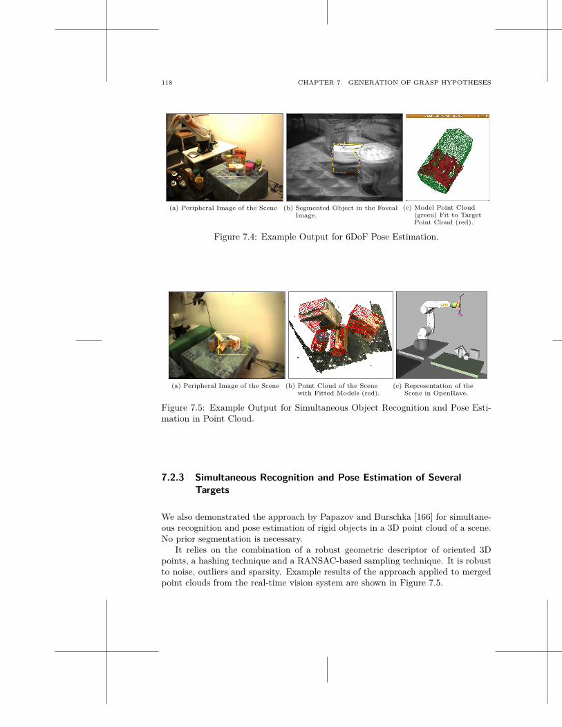
118 CHAPTER 7. GENERATION OF GRASP HYPOTHESES
(a) Peripheral Image of the Scene (b) Segmented Object in the FovealImage.
(c) Model Point Cloud(green) Fit to TargetPoint Cloud (red).
Figure 7.4: Example Output for 6DoF Pose Estimation.
(a) Peripheral Image of the Scene (b) Point Cloud of the Scenewith Fitted Models (red).
(c) Representation of theScene in OpenRave.
Figure 7.5: Example Output for Simultaneous Object Recognition and Pose Esti-mation in Point Cloud.
7.2.3 Simultaneous Recognition and Pose Estimation of Several
Targets
We also demonstrated the approach by Papazov and Burschka [166] for simultane-ous recognition and pose estimation of rigid objects in a 3D point cloud of a scene.No prior segmentation is necessary.
It relies on the combination of a robust geometric descriptor of oriented 3Dpoints, a hashing technique and a RANSAC-based sampling technique. It is robustto noise, outliers and sparsity. Example results of the approach applied to mergedpoint clouds from the real-time vision system are shown in Figure 7.5.
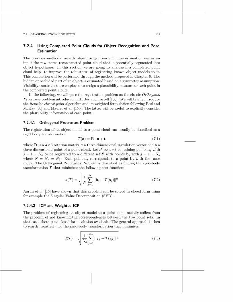
7.2. GRASPING KNOWN OBJECTS 119
7.2.4 Using Completed Point Clouds for Object Recognition and Pose
Estimation
The previous methods towards object recognition and pose estimation use as aninput the raw stereo reconstructed point cloud that is potentially segmented intoobject hypotheses. In this section we are going to analyse if a completed pointcloud helps to improve the robustness of registering known object models to it.This completion will be performed through the method proposed in Chapter 6. Thehidden or occluded part of an object is estimated based on a symmetry assumption.Visibility constraints are employed to assign a plausibility measure to each point inthe completed point cloud.
In the following, we will pose the registration problem as the classic OrthogonalProcrustes problem introduced in Hurley and Cartell [103]. We will briefly introducethe iterative closest point algorithm and its weighted formulation following Besl andMcKay [30] and Maurer et al. [150]. The latter will be useful to explicitly considerthe plausibility information of each point.
7.2.4.1 Orthogonal Procrustes Problem
The registration of an object model to a point cloud can usually be described as arigid body transformation
T (a) = R · a + t (7.1)
where R is a 3×3 rotation matrix, t a three-dimensional translation vector and a athree-dimensional point of a point cloud. Let A be a set containing points aj withj = 1 . . . Na to be registered to a different set B with points bj with j = 1 . . . Nb
where N = Na = Nb. Each point aj corresponds to a point bj with the sameindex. The Orthogonal Procrustes Problem is described as finding the rigid-bodytransformation T that minimises the following cost function:
d(T ) =
√
√
√
√
1N
N∑
j=1
||bj − T (aj)||2 (7.2)
Aarun et al. [15] have shown that this problem can be solved in closed form usingfor example the Singular Value Decomposition (SVD).
7.2.4.2 ICP and Weighted ICP
The problem of registering an object model to a point cloud usually suffers fromthe problem of not knowing the correspondences between the two point sets. Inthat case, there is no closed-form solution available. The general approach is thento search iteratively for the rigid-body transformation that minimises
d(T ) =
√
√
√
√
1Na
Na∑
j=1
||yj − T (aj)||2 (7.3)
120 CHAPTER 7. GENERATION OF GRASP HYPOTHESES
whereyj = c(T (aj), B) (7.4)
is a point in the point set B that corresponds to point aj . This relation is determinedthrough the correspondence function c(·)
Besl and McKay [30] proposed ICP in which c(·) is the closest point operator.They showed that their method converges to the local minimum of the cost functionin Equation 7.3.
Maurer et al. [150] proposed a weighted extension of the original ICP method.Let W be a set of weights wj with j = 1 . . . Na associated with the points in A.The authors show that their weighted ICP formulation minimises the following costfunction:
d(T ) =
√
√
√
√
1Na
Na∑
j=1
wj ||yj − T (aj)||2 (7.5)
where the function c(·) is defined as in Equation 7.4.
ICP for Completed Point Clouds In this section, we propose to register thetrue object model to the completed point cloud instead of to the partial one. Ourhypothesis is that this increases the robustness of fitting because more points thatconstrain the pose of the true object are available.
We use ICP as implemented in [193] that iteratively minimises Equation 7.3.The set B consist of the completed point cloud. A contains point samples fromthe surface of the ground truth object. The mesh is sampled using the methoddescribed in Roy et al. [189].
Using Plausibility Information for Registration The quality of the ICP-based registration of the object model to the completed point cloud depends on thequality of the symmetry plane estimation. The resulting point cloud might divergestrongly from the true shape. Therefore, we want to ensure that the registeredmodel complies more accurately to the original reconstructed points than to thehypothesized ones.
We approach this, by using a weighted ICP scheme proposed in Maurer et al.[150] that minimises the cost function in Equation 7.5. B consists of the completedpoint cloud and A of the sampled ground truth mesh. As weights wj , we choose theplausibility plaus(bj) of each point bj in the set B. This is defined in Equation 6.3and 6.4.
We implemented this approach by adapting ICP from [193] as shown in Algo-rithm 3.
7.2.4.3 Experiments
In this section, we want to evaluate the proposed approach of using the completedpoint clouds as targets for the registration of ground truth object models. Our
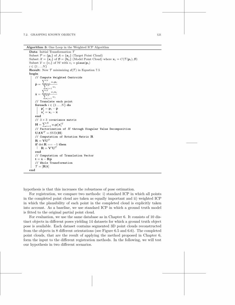
7.2. GRASPING KNOWN OBJECTS 121
Algorithm 3: One Loop in the Weighted ICP Algorithm
Data: Initial Transformation TSubset P = {pi} of A = {aj} (Target Point Cloud)Subset X = {xi} of B = {bj} (Model Point Cloud) where xi = C(T (pi), B)Subset V = {vi} of W with vi = plaus(pi)i ∈ {1 . . . N}Result: New T minimizing d(T ) in Equation 7.5begin
// Compute Weighted Centroids
p =
∑
N
i=1wipi
∑
N
j=1wi
x =
∑
N
i=1wixi
∑
N
j=1wi
// Translate each point
foreach i ∈ {1 . . . N} dop′
i= pi − p
x′
i= xi − x
end
// 3 × 3 covariance matrix
H =∑N
i=1wip
′
ix′T
i
// Factorization of H through Singular Value Decomposition
UΛVT = SVD(H)// Computation of Rotation Matrix R
R = VUT
if det R == −1 then
R = V′UT
end
// Computation of Translation Vector
t = x − Rp
// Whole Transformation
T = [R|t]end
hypothesis is that this increases the robustness of pose estimation.For registration, we compare two methods: i) standard ICP in which all points
in the completed point cloud are taken as equally important and ii) weighted ICPin which the plausibility of each point in the completed cloud is explicitly takeninto account. As a baseline, we use standard ICP in which a ground truth modelis fitted to the original partial point cloud.
For evaluation, we use the same database as in Chapter 6. It consists of 10 dis-tinct objects in different poses yielding 14 datasets for which a ground truth objectpose is available. Each dataset contains segmented 3D point clouds reconstructedfrom the objects in 8 different orientations (see Figure 6.5 and 6.6). The completedpoint clouds, that are the result of applying the method proposed in Chapter 6,form the input to the different registration methods. In the following, we will testour hypothesis in two different scenarios.
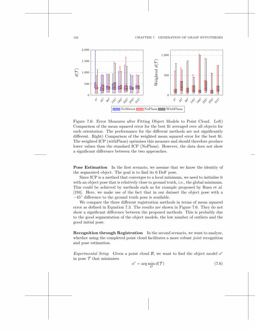
122 CHAPTER 7. GENERATION OF GRASP HYPOTHESES
0◦
45◦
90◦
135◦
180◦
225◦
270◦
315◦
0
500
1,000
1,500
2,000
d(T
)
0◦
45◦
90◦
135◦
180◦
225◦
270◦
315◦
0
500
1,000
Wei
ghte
dd(T
)
NoMirror NoPlaus WithPlaus
Figure 7.6: Error Measures after Fitting Object Models to Point Cloud. Left)Comparison of the mean squared error for the best fit averaged over all objects foreach orientation. The performance for the different methods are not significantlydifferent. Right) Comparison of the weighted mean squared error for the best fit.The weighted ICP (withPlaus) optimises this measure and should therefore producelower values than the standard ICP (NoPlaus). However, the data does not showa significant difference between the two approaches.
Pose Estimation In the first scenario, we assume that we know the identity ofthe segmented object. The goal is to find its 6 DoF pose.
Since ICP is a method that converges to a local minimum, we need to initialise itwith an object pose that is relatively close to ground truth, i.e., the global minimum.This could be achieved by methods such as for example proposed by Rusu et al.[194]. Here, we make use of the fact that in our dataset the object pose with a−45◦ difference to the ground truth pose is available.
We compare the three different registration methods in terms of mean squarederror as defined in Equation 7.3. The results are shown in Figure 7.6. They do notshow a significant difference between the proposed methods. This is probably dueto the good segmentation of the object models, the low number of outliers and thegood initial pose.
Recognition through Registration In the second scenario, we want to analyse,whether using the completed point cloud facilitates a more robust joint recognitionand pose estimation.
Experimental Setup Given a point cloud B, we want to find the object model o∗
in pose T that minimiseso∗ = arg min
Od(T ) (7.6)
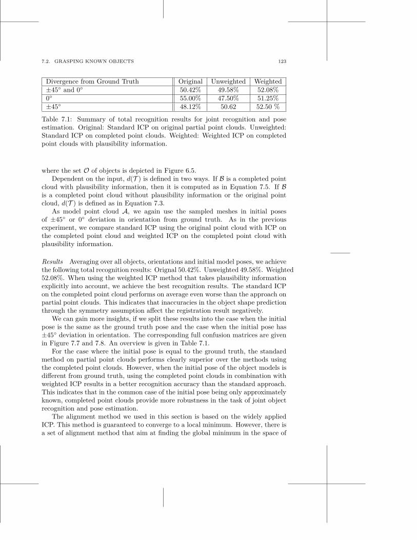
7.2. GRASPING KNOWN OBJECTS 123
Divergence from Ground Truth Original Unweighted Weighted±45◦ and 0◦ 50.42% 49.58% 52.08%0◦ 55.00% 47.50% 51.25%±45◦ 48.12% 50.62 52.50 %
Table 7.1: Summary of total recognition results for joint recognition and poseestimation. Original: Standard ICP on original partial point clouds. Unweighted:Standard ICP on completed point clouds. Weighted: Weighted ICP on completedpoint clouds with plausibility information.
where the set O of objects is depicted in Figure 6.5.Dependent on the input, d(T ) is defined in two ways. If B is a completed point
cloud with plausibility information, then it is computed as in Equation 7.5. If Bis a completed point cloud without plausibility information or the original pointcloud, d(T ) is defined as in Equation 7.3.
As model point cloud A, we again use the sampled meshes in initial posesof ±45◦ or 0◦ deviation in orientation from ground truth. As in the previousexperiment, we compare standard ICP using the original point cloud with ICP onthe completed point cloud and weighted ICP on the completed point cloud withplausibility information.
Results Averaging over all objects, orientations and initial model poses, we achievethe following total recognition results: Orignal 50.42%. Unweighted 49.58%. Weighted52.08%. When using the weighted ICP method that takes plausibility informationexplicitly into account, we achieve the best recognition results. The standard ICPon the completed point cloud performs on average even worse than the approach onpartial point clouds. This indicates that inaccuracies in the object shape predictionthrough the symmetry assumption affect the registration result negatively.
We can gain more insights, if we split these results into the case when the initialpose is the same as the ground truth pose and the case when the initial pose has±45◦ deviation in orientation. The corresponding full confusion matrices are givenin Figure 7.7 and 7.8. An overview is given in Table 7.1.
For the case where the initial pose is equal to the ground truth, the standardmethod on partial point clouds performs clearly superior over the methods usingthe completed point clouds. However, when the initial pose of the object models isdifferent from ground truth, using the completed point clouds in combination withweighted ICP results in a better recognition accuracy than the standard approach.This indicates that in the common case of the initial pose being only approximatelyknown, completed point clouds provide more robustness in the task of joint objectrecognition and pose estimation.
The alignment method we used in this section is based on the widely appliedICP. This method is guaranteed to converge to a local minimum. However, there isa set of alignment method that aim at finding the global minimum in the space of
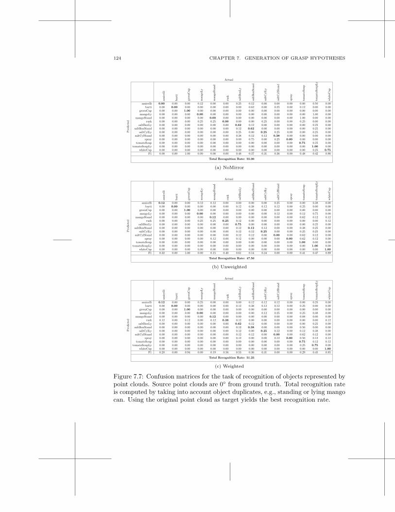
124 CHAPTER 7. GENERATION OF GRASP HYPOTHESES
Actual
amic
elli
burt
i
gree
nCup
man
goL
y
man
goSt
and
rusk
salt
Box
Ly
salt
Box
Stan
d
salt
Cyl
Ly
salt
Cyl
Stan
d
spra
y
tom
atoS
oup
tom
atoS
oupL
y
whi
teC
up
Pre
dict
ed
amicelli 0.00 0.00 0.00 0.12 0.00 0.00 0.25 0.12 0.00 0.00 0.00 0.00 0.50 0.00burti 0.00 0.00 0.00 0.00 0.00 0.00 0.00 0.62 0.00 0.25 0.00 0.12 0.00 0.00
greenCup 0.00 0.00 1.00 0.00 0.00 0.00 0.00 0.00 0.00 0.00 0.00 0.00 0.00 0.00mangoLy 0.00 0.00 0.00 0.00 0.00 0.00 0.00 0.00 0.00 0.00 0.00 0.00 1.00 0.00
mangoStand 0.00 0.00 0.00 0.00 0.00 0.00 0.00 0.00 0.00 0.00 0.00 1.00 0.00 0.00rusk 0.00 0.00 0.00 0.25 0.25 0.00 0.00 0.00 0.25 0.00 0.00 0.25 0.00 0.00
saltBoxLy 0.00 0.00 0.00 0.00 0.00 0.00 0.62 0.12 0.00 0.00 0.00 0.00 0.25 0.00saltBoxStand 0.00 0.00 0.00 0.00 0.00 0.00 0.12 0.62 0.00 0.00 0.00 0.00 0.25 0.00
saltCylLy 0.00 0.00 0.00 0.00 0.00 0.00 0.25 0.00 0.25 0.25 0.00 0.00 0.25 0.00saltCylStand 0.00 0.00 0.00 0.00 0.00 0.00 0.38 0.12 0.12 0.38 0.00 0.00 0.00 0.00
spray 0.00 0.00 0.00 0.00 0.00 0.00 0.00 0.75 0.00 0.25 0.00 0.00 0.00 0.00tomatoSoup 0.00 0.00 0.00 0.00 0.00 0.00 0.00 0.00 0.00 0.00 0.00 0.75 0.25 0.00
tomatoSoupLy 0.00 0.00 0.00 0.00 0.00 0.00 0.00 0.00 0.00 0.00 0.00 0.00 1.00 0.00whiteCup 0.00 0.00 0.00 0.00 0.00 0.00 0.00 0.00 0.00 0.00 0.00 0.00 0.25 0.75
F1 0.00 0.00 1.00 0.00 0.00 0.00 0.48 0.37 0.31 0.36 0.00 0.48 0.42 0.86
Total Recognition Rate: 55.00
(a) NoMirror
Actual
amic
elli
burt
i
gree
nCup
man
goL
y
man
goSt
and
rusk
salt
Box
Ly
salt
Box
Stan
d
salt
Cyl
Ly
salt
Cyl
Stan
d
spra
y
tom
atoS
oup
tom
atoS
oupL
y
whi
teC
up
Pre
dict
ed
amicelli 0.12 0.00 0.00 0.12 0.12 0.00 0.00 0.00 0.00 0.25 0.00 0.00 0.38 0.00burti 0.00 0.00 0.00 0.00 0.00 0.00 0.12 0.38 0.12 0.12 0.00 0.25 0.00 0.00
greenCup 0.00 0.00 1.00 0.00 0.00 0.00 0.00 0.00 0.00 0.00 0.00 0.00 0.00 0.00mangoLy 0.00 0.00 0.00 0.00 0.00 0.00 0.00 0.00 0.00 0.12 0.00 0.12 0.75 0.00
mangoStand 0.00 0.00 0.00 0.00 0.12 0.00 0.00 0.00 0.00 0.00 0.00 0.62 0.12 0.12rusk 0.00 0.00 0.00 0.25 0.25 0.25 0.12 0.00 0.00 0.00 0.00 0.00 0.00 0.12
saltBoxLy 0.00 0.00 0.00 0.00 0.00 0.00 0.75 0.00 0.00 0.00 0.00 0.00 0.25 0.00saltBoxStand 0.00 0.00 0.00 0.00 0.00 0.00 0.12 0.12 0.12 0.00 0.00 0.38 0.25 0.00
saltCylLy 0.00 0.00 0.00 0.00 0.00 0.00 0.12 0.12 0.25 0.00 0.00 0.25 0.25 0.00saltCylStand 0.00 0.00 0.00 0.00 0.00 0.00 0.12 0.12 0.00 0.00 0.00 0.62 0.12 0.00
spray 0.00 0.00 0.00 0.00 0.12 0.00 0.12 0.00 0.00 0.00 0.00 0.62 0.12 0.00tomatoSoup 0.00 0.00 0.00 0.00 0.00 0.00 0.00 0.00 0.00 0.00 0.00 1.00 0.00 0.00
tomatoSoupLy 0.00 0.00 0.00 0.00 0.00 0.00 0.00 0.00 0.00 0.00 0.00 0.00 1.00 0.00whiteCup 0.00 0.00 0.00 0.00 0.00 0.00 0.00 0.00 0.00 0.00 0.00 0.00 0.00 1.00
F1 0.22 0.00 1.00 0.00 0.15 0.40 0.61 0.14 0.34 0.00 0.00 0.41 0.47 0.89
Total Recognition Rate: 47.50
(b) Unweighted
Actual
amic
elli
burt
i
gree
nCup
man
goL
y
man
goSt
and
rusk
salt
Box
Ly
salt
Box
Stan
d
salt
Cyl
Ly
salt
Cyl
Stan
d
spra
y
tom
atoS
oup
tom
atoS
oupL
y
whi
teC
up
Pre
dict
ed
amicelli 0.12 0.00 0.00 0.25 0.00 0.00 0.00 0.12 0.12 0.12 0.00 0.00 0.25 0.00burti 0.00 0.00 0.00 0.00 0.00 0.00 0.12 0.38 0.12 0.12 0.00 0.25 0.00 0.00
greenCup 0.00 0.00 1.00 0.00 0.00 0.00 0.00 0.00 0.00 0.00 0.00 0.00 0.00 0.00mangoLy 0.00 0.00 0.00 0.00 0.00 0.00 0.00 0.00 0.12 0.25 0.00 0.25 0.38 0.00
mangoStand 0.00 0.00 0.00 0.00 0.12 0.00 0.00 0.00 0.00 0.00 0.00 0.88 0.00 0.00rusk 0.12 0.00 0.12 0.00 0.12 0.38 0.12 0.00 0.00 0.00 0.00 0.00 0.00 0.12
saltBoxLy 0.00 0.00 0.00 0.00 0.00 0.00 0.62 0.12 0.00 0.00 0.00 0.00 0.25 0.00saltBoxStand 0.00 0.00 0.00 0.00 0.00 0.00 0.12 0.38 0.00 0.00 0.00 0.50 0.00 0.00
saltCylLy 0.00 0.00 0.00 0.00 0.00 0.00 0.12 0.00 0.25 0.12 0.00 0.12 0.38 0.00saltCylStand 0.00 0.00 0.00 0.00 0.00 0.00 0.12 0.12 0.00 0.00 0.00 0.62 0.12 0.00
spray 0.00 0.00 0.00 0.00 0.00 0.00 0.12 0.00 0.00 0.12 0.00 0.50 0.12 0.12tomatoSoup 0.00 0.00 0.00 0.00 0.00 0.00 0.00 0.00 0.00 0.00 0.00 0.75 0.12 0.12
tomatoSoupLy 0.00 0.00 0.00 0.00 0.00 0.00 0.00 0.00 0.00 0.00 0.00 0.25 0.75 0.00whiteCup 0.00 0.00 0.00 0.00 0.00 0.00 0.00 0.00 0.00 0.00 0.00 0.00 0.00 1.00
F1 0.20 0.00 0.94 0.00 0.19 0.56 0.53 0.36 0.31 0.00 0.00 0.29 0.45 0.85
Total Recognition Rate: 51.25
(c) Weighted
Figure 7.7: Confusion matrices for the task of recognition of objects represented bypoint clouds. Source point clouds are 0◦ from ground truth. Total recognition rateis computed by taking into account object duplicates, e.g., standing or lying mangocan. Using the original point cloud as target yields the best recognition rate.
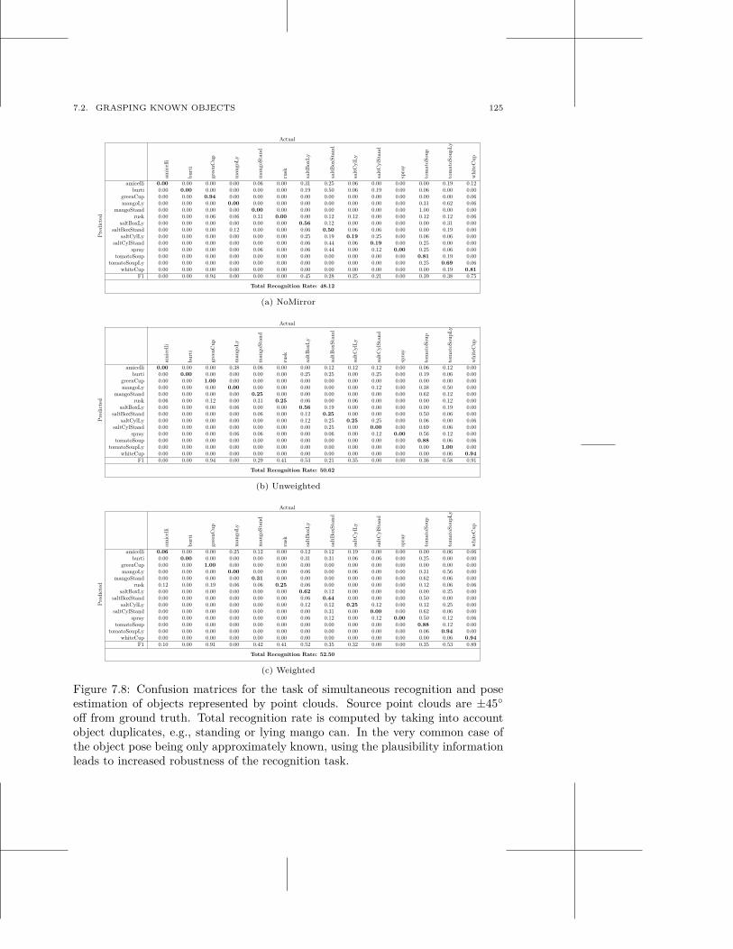
7.2. GRASPING KNOWN OBJECTS 125
Actual
amic
elli
burt
i
gree
nCup
man
goL
y
man
goSt
and
rusk
salt
Box
Ly
salt
Box
Stan
d
salt
Cyl
Ly
salt
Cyl
Stan
d
spra
y
tom
atoS
oup
tom
atoS
oupL
y
whi
teC
up
Pre
dict
ed
amicelli 0.00 0.00 0.00 0.00 0.06 0.00 0.31 0.25 0.06 0.00 0.00 0.00 0.19 0.12burti 0.00 0.00 0.00 0.00 0.00 0.00 0.19 0.50 0.06 0.19 0.00 0.06 0.00 0.00
greenCup 0.00 0.00 0.94 0.00 0.00 0.00 0.00 0.00 0.00 0.00 0.00 0.00 0.00 0.06mangoLy 0.00 0.00 0.00 0.00 0.00 0.00 0.00 0.00 0.00 0.00 0.00 0.31 0.62 0.06
mangoStand 0.00 0.00 0.00 0.00 0.00 0.00 0.00 0.00 0.00 0.00 0.00 1.00 0.00 0.00rusk 0.00 0.00 0.06 0.06 0.31 0.00 0.00 0.12 0.12 0.00 0.00 0.12 0.12 0.06
saltBoxLy 0.00 0.00 0.00 0.00 0.00 0.00 0.56 0.12 0.00 0.00 0.00 0.00 0.31 0.00saltBoxStand 0.00 0.00 0.00 0.12 0.00 0.00 0.06 0.50 0.06 0.06 0.00 0.00 0.19 0.00
saltCylLy 0.00 0.00 0.00 0.00 0.00 0.00 0.25 0.19 0.19 0.25 0.00 0.06 0.06 0.00saltCylStand 0.00 0.00 0.00 0.00 0.00 0.00 0.06 0.44 0.06 0.19 0.00 0.25 0.00 0.00
spray 0.00 0.00 0.00 0.00 0.06 0.00 0.06 0.44 0.00 0.12 0.00 0.25 0.06 0.00tomatoSoup 0.00 0.00 0.00 0.00 0.00 0.00 0.00 0.00 0.00 0.00 0.00 0.81 0.19 0.00
tomatoSoupLy 0.00 0.00 0.00 0.00 0.00 0.00 0.00 0.00 0.00 0.00 0.00 0.25 0.69 0.06whiteCup 0.00 0.00 0.00 0.00 0.00 0.00 0.00 0.00 0.00 0.00 0.00 0.00 0.19 0.81
F1 0.00 0.00 0.94 0.00 0.00 0.00 0.45 0.28 0.25 0.21 0.00 0.39 0.38 0.75
Total Recognition Rate: 48.12
(a) NoMirror
Actual
amic
elli
burt
i
gree
nCup
man
goL
y
man
goSt
and
rusk
salt
Box
Ly
salt
Box
Stan
d
salt
Cyl
Ly
salt
Cyl
Stan
d
spra
y
tom
atoS
oup
tom
atoS
oupL
y
whi
teC
up
Pre
dict
ed
amicelli 0.00 0.00 0.00 0.38 0.06 0.00 0.00 0.12 0.12 0.12 0.00 0.06 0.12 0.00burti 0.00 0.00 0.00 0.00 0.00 0.00 0.25 0.25 0.00 0.25 0.00 0.19 0.06 0.00
greenCup 0.00 0.00 1.00 0.00 0.00 0.00 0.00 0.00 0.00 0.00 0.00 0.00 0.00 0.00mangoLy 0.00 0.00 0.00 0.00 0.00 0.00 0.00 0.00 0.00 0.12 0.00 0.38 0.50 0.00
mangoStand 0.00 0.00 0.00 0.00 0.25 0.00 0.00 0.00 0.00 0.00 0.00 0.62 0.12 0.00rusk 0.06 0.00 0.12 0.00 0.31 0.25 0.06 0.00 0.06 0.00 0.00 0.00 0.12 0.00
saltBoxLy 0.00 0.00 0.00 0.06 0.00 0.00 0.56 0.19 0.00 0.00 0.00 0.00 0.19 0.00saltBoxStand 0.00 0.00 0.00 0.00 0.06 0.00 0.12 0.25 0.00 0.00 0.00 0.50 0.06 0.00
saltCylLy 0.00 0.00 0.00 0.00 0.00 0.00 0.12 0.25 0.25 0.25 0.00 0.06 0.00 0.06saltCylStand 0.00 0.00 0.00 0.00 0.00 0.00 0.00 0.25 0.00 0.00 0.00 0.69 0.06 0.00
spray 0.00 0.00 0.00 0.06 0.06 0.00 0.00 0.06 0.00 0.12 0.00 0.56 0.12 0.00tomatoSoup 0.00 0.00 0.00 0.00 0.00 0.00 0.00 0.00 0.00 0.00 0.00 0.88 0.06 0.06
tomatoSoupLy 0.00 0.00 0.00 0.00 0.00 0.00 0.00 0.00 0.00 0.00 0.00 0.00 1.00 0.00whiteCup 0.00 0.00 0.00 0.00 0.00 0.00 0.00 0.00 0.00 0.00 0.00 0.00 0.06 0.94
F1 0.00 0.00 0.94 0.00 0.29 0.41 0.53 0.21 0.35 0.00 0.00 0.36 0.58 0.91
Total Recognition Rate: 50.62
(b) Unweighted
Actual
amic
elli
burt
i
gree
nCup
man
goL
y
man
goSt
and
rusk
salt
Box
Ly
salt
Box
Stan
d
salt
Cyl
Ly
salt
Cyl
Stan
d
spra
y
tom
atoS
oup
tom
atoS
oupL
y
whi
teC
up
Pre
dict
ed
amicelli 0.06 0.00 0.00 0.25 0.12 0.00 0.12 0.12 0.19 0.00 0.00 0.00 0.06 0.06burti 0.00 0.00 0.00 0.00 0.00 0.00 0.31 0.31 0.06 0.06 0.00 0.25 0.00 0.00
greenCup 0.00 0.00 1.00 0.00 0.00 0.00 0.00 0.00 0.00 0.00 0.00 0.00 0.00 0.00mangoLy 0.00 0.00 0.00 0.00 0.00 0.00 0.06 0.00 0.06 0.00 0.00 0.31 0.56 0.00
mangoStand 0.00 0.00 0.00 0.00 0.31 0.00 0.00 0.00 0.00 0.00 0.00 0.62 0.06 0.00rusk 0.12 0.00 0.19 0.06 0.06 0.25 0.06 0.00 0.00 0.00 0.00 0.12 0.06 0.06
saltBoxLy 0.00 0.00 0.00 0.00 0.00 0.00 0.62 0.12 0.00 0.00 0.00 0.00 0.25 0.00saltBoxStand 0.00 0.00 0.00 0.00 0.00 0.00 0.06 0.44 0.00 0.00 0.00 0.50 0.00 0.00
saltCylLy 0.00 0.00 0.00 0.00 0.00 0.00 0.12 0.12 0.25 0.12 0.00 0.12 0.25 0.00saltCylStand 0.00 0.00 0.00 0.00 0.00 0.00 0.00 0.31 0.00 0.00 0.00 0.62 0.06 0.00
spray 0.00 0.00 0.00 0.00 0.00 0.00 0.06 0.12 0.00 0.12 0.00 0.50 0.12 0.06tomatoSoup 0.00 0.00 0.00 0.00 0.00 0.00 0.00 0.00 0.00 0.00 0.00 0.88 0.12 0.00
tomatoSoupLy 0.00 0.00 0.00 0.00 0.00 0.00 0.00 0.00 0.00 0.00 0.00 0.06 0.94 0.00whiteCup 0.00 0.00 0.00 0.00 0.00 0.00 0.00 0.00 0.00 0.00 0.00 0.00 0.06 0.94
F1 0.10 0.00 0.91 0.00 0.42 0.41 0.52 0.35 0.32 0.00 0.00 0.35 0.53 0.89
Total Recognition Rate: 52.50
(c) Weighted
Figure 7.8: Confusion matrices for the task of simultaneous recognition and poseestimation of objects represented by point clouds. Source point clouds are ±45◦
off from ground truth. Total recognition rate is computed by taking into accountobject duplicates, e.g., standing or lying mango can. In the very common case ofthe object pose being only approximately known, using the plausibility informationleads to increased robustness of the recognition task.
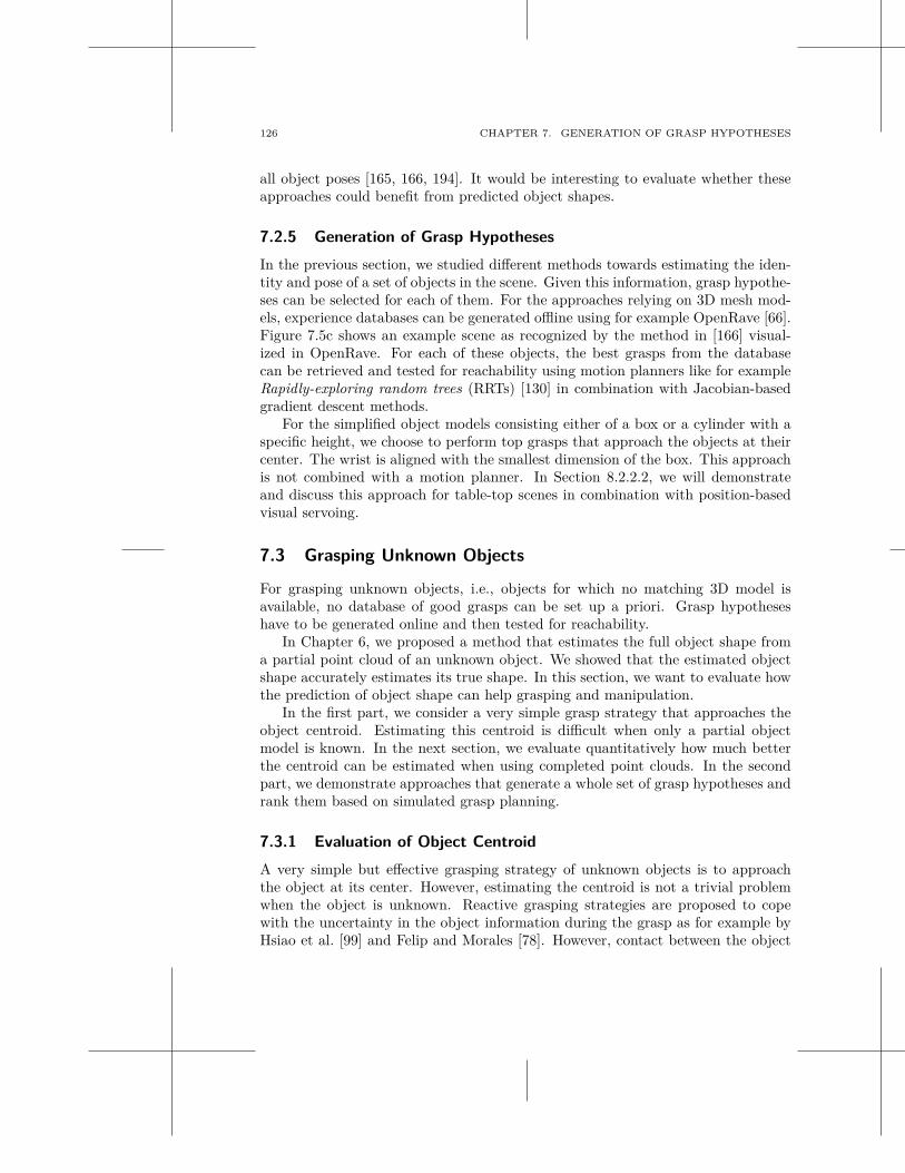
126 CHAPTER 7. GENERATION OF GRASP HYPOTHESES
all object poses [165, 166, 194]. It would be interesting to evaluate whether theseapproaches could benefit from predicted object shapes.
7.2.5 Generation of Grasp Hypotheses
In the previous section, we studied different methods towards estimating the iden-tity and pose of a set of objects in the scene. Given this information, grasp hypothe-ses can be selected for each of them. For the approaches relying on 3D mesh mod-els, experience databases can be generated offline using for example OpenRave [66].Figure 7.5c shows an example scene as recognized by the method in [166] visual-ized in OpenRave. For each of these objects, the best grasps from the databasecan be retrieved and tested for reachability using motion planners like for exampleRapidly-exploring random trees (RRTs) [130] in combination with Jacobian-basedgradient descent methods.
For the simplified object models consisting either of a box or a cylinder with aspecific height, we choose to perform top grasps that approach the objects at theircenter. The wrist is aligned with the smallest dimension of the box. This approachis not combined with a motion planner. In Section 8.2.2.2, we will demonstrateand discuss this approach for table-top scenes in combination with position-basedvisual servoing.
7.3 Grasping Unknown Objects
For grasping unknown objects, i.e., objects for which no matching 3D model isavailable, no database of good grasps can be set up a priori. Grasp hypotheseshave to be generated online and then tested for reachability.
In Chapter 6, we proposed a method that estimates the full object shape froma partial point cloud of an unknown object. We showed that the estimated objectshape accurately estimates its true shape. In this section, we want to evaluate howthe prediction of object shape can help grasping and manipulation.
In the first part, we consider a very simple grasp strategy that approaches theobject centroid. Estimating this centroid is difficult when only a partial objectmodel is known. In the next section, we evaluate quantitatively how much betterthe centroid can be estimated when using completed point clouds. In the secondpart, we demonstrate approaches that generate a whole set of grasp hypotheses andrank them based on simulated grasp planning.
7.3.1 Evaluation of Object Centroid
A very simple but effective grasping strategy of unknown objects is to approachthe object at its center. However, estimating the centroid is not a trivial problemwhen the object is unknown. Reactive grasping strategies are proposed to copewith the uncertainty in the object information during the grasp as for example byHsiao et al. [99] and Felip and Morales [78]. However, contact between the object
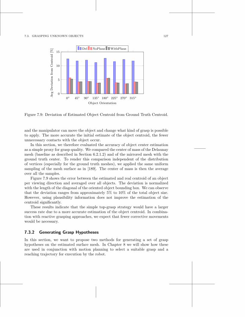
7.3. GRASPING UNKNOWN OBJECTS 127
0◦ 45◦ 90◦ 135◦ 180◦ 225◦ 270◦ 315◦
0
5
10
15
Object Orientation
Av
gD
evia
tion
from
Cen
troid
[%] Del NoPlaus WithPlaus
Figure 7.9: Deviation of Estimated Object Centroid from Ground Truth Centroid.
and the manipulator can move the object and change what kind of grasp is possibleto apply. The more accurate the initial estimate of the object centroid, the fewerunnecessary contacts with the object occur.
In this section, we therefore evaluated the accuracy of object center estimationas a simple proxy for grasp quality. We compared the center of mass of the Delaunaymesh (baseline as described in Section 6.2.1.2) and of the mirrored mesh with theground truth center. To render this comparison independent of the distributionof vertices (especially for the ground truth meshes), we applied the same uniformsampling of the mesh surface as in [189]. The center of mass is then the averageover all the samples.
Figure 7.9 shows the error between the estimated and real centroid of an objectper viewing direction and averaged over all objects. The deviation is normalizedwith the length of the diagonal of the oriented object bounding box. We can observethat the deviation ranges from approximately 5% to 10% of the total object size.However, using plausibility information does not improve the estimation of thecentroid significantly.
These results indicate that the simple top-grasp strategy would have a largersuccess rate due to a more accurate estimation of the object centroid. In combina-tion with reactive grasping approaches, we expect that fewer corrective movementswould be necessary.
7.3.2 Generating Grasp Hypotheses
In this section, we want to propose two methods for generating a set of grasphypotheses on the estimated surface mesh. In Chapter 8 we will show how theseare used in conjunction with motion planning to select a suitable grasp and areaching trajectory for execution by the robot.
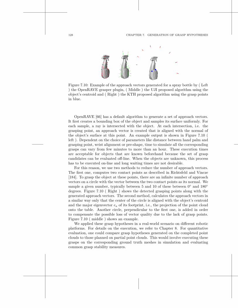
128 CHAPTER 7. GENERATION OF GRASP HYPOTHESES
Figure 7.10: Example of the approach vectors generated for a spray bottle by ( Left) the OpenRAVE grasper plugin, ( Middle ) the UJI proposed algorithm using theobject’s centroid and ( Right ) the KTH proposed algorithm using the grasp pointsin blue.
OpenRAVE [66] has a default algorithm to generate a set of approach vectors.It first creates a bounding box of the object and samples its surface uniformly. Foreach sample, a ray is intersected with the object. At each intersection, i.e. thegrasping point, an approach vector is created that is aligned with the normal ofthe object’s surface at this point. An example output is shown in Figure 7.10 (left ). Dependent on the choice of parameters like distance between hand palm andgrasping point, wrist alignment or pre-shape, time to simulate all the correspondinggrasps can vary from few minutes to more than an hour. These execution timesare acceptable for objects that are known beforehand because the set of graspcandidates can be evaluated off-line. When the objects are unknown, this processhas to be executed on-line and long waiting times are not desirable.
For this reason, we use two methods to reduce the number of approach vectors.The first one, computes two contact points as described in Richtsfeld and Vincze[184]. To grasp the object at these points, there are an infinite number of approachvectors on a circle with the vector between the two contact points as its normal. Wesample a given number, typically between 5 and 10 of these between 0◦ and 180◦
degrees. Figure 7.10 ( Right ) shows the detected grasping points along with thegenerated approach vectors. The second method, calculates the approach vectors ina similar way only that the center of the circle is aligned with the object’s centroidand the major eigenvector ea of its footprint, i.e., the projection of the point cloudonto the table. Another circle, perpendicular to the first one, is added in orderto compensate the possible loss of vector quality due to the lack of grasp points.Figure 7.10 ( middle ) shows an example.
We applied these grasp hypotheses in a real-world scenario on different roboticplatforms. For details on the execution, we refer to Chapter 8. For quantitativeevaluation, one could compare grasp hypotheses generated on the completed pointclouds to those planned on partial point clouds. This would involve executing thesegrasps on the corresponding ground truth meshes in simulation and evaluatingcommon grasp stability measures.
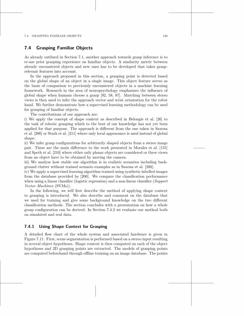
7.4. GRASPING FAMILIAR OBJECTS 129
7.4 Grasping Familiar Objects
As already outlined in Section 7.1, another approach towards grasp inference is tore-use prior grasping experience on familiar objects. A similarity metric betweenalready encountered objects and new ones has to be developed that takes grasp-relevant features into account.
In the approach proposed in this section, a grasping point is detected basedon the global shape of an object in a single image. This object feature serves asthe basis of comparison to previously encountered objects in a machine learningframework. Research in the area of neuropsychology emphasizes the influence ofglobal shape when humans choose a grasp [92, 58, 87]. Matching between stereoviews is then used to infer the approach vector and wrist orientation for the robothand. We further demonstrate how a supervised learning methodology can be usedfor grasping of familiar objects.
The contributions of our approach are:i) We apply the concept of shape context as described in Belongie et al. [26] tothe task of robotic grasping which to the best of our knowledge has not yet beenapplied for that purpose. The approach is different from the one taken in Saxenaet al. [200] or Stark et al. [211] where only local appearance is used instead of globalshape.ii) We infer grasp configurations for arbitrarily shaped objects from a stereo imagepair. These are the main difference to the work presented in Morales et al. [155]and Speth et al. [210] where either only planar objects are considered or three viewsfrom an object have to be obtained by moving the camera.iii) We analyse how stable our algorithm is in realistic scenarios including back-ground clutter without trained scenario examples as in Saxena et al. [200].iv) We apply a supervised learning algorithm trained using synthetic labelled imagesfrom the database provided by [200]. We compare the classification performancewhen using a linear classifier (logistic regression) and a non-linear classifier (SupportVector Machines (SVMs)).
In the following, we will first describe the method of applying shape contextto grasping is introduced. We also describe and comment on the database thatwe used for training and give some background knowledge on the two differentclassification methods. The section concludes with a presentation on how a wholegrasp configuration can be derived. In Section 7.4.2 we evaluate our method bothon simulated and real data.
7.4.1 Using Shape Context for Grasping
A detailed flow chart of the whole system and associated hardware is given inFigure 7.11. First, scene segmentation is performed based on a stereo input resultingin several object hypotheses. Shape context is then computed on each of the objecthypotheses and 2D grasping points are extracted. The models of grasping pointsare computed beforehand through offline training on an image database. The points
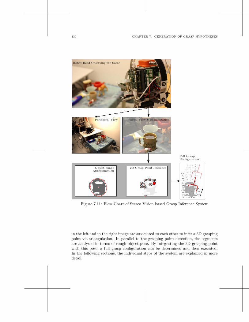
130 CHAPTER 7. GENERATION OF GRASP HYPOTHESES
Robot Head Observing the Scene
Peripheral View Foveal View & Segmentation
Object ShapeApproximation
2D Grasp Point Inference
Full GraspConfiguration
Figure 7.11: Flow Chart of Stereo Vision based Grasp Inference System
in the left and in the right image are associated to each other to infer a 3D graspingpoint via triangulation. In parallel to the grasping point detection, the segmentsare analysed in terms of rough object pose. By integrating the 3D grasping pointwith this pose, a full grasp configuration can be determined and then executed.In the following sections, the individual steps of the system are explained in moredetail.
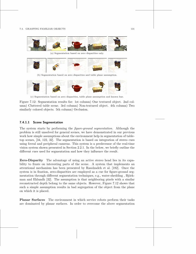
7.4. GRASPING FAMILIAR OBJECTS 131
(a) Segmentation based on zero disparities only.
(b) Segmentation based on zero disparities and table plane assumption.
(c) Segmentation based on zero disparities, table plane assumption and known hue.
Figure 7.12: Segmentation results for: 1st column) One textured object. 2nd col-umn) Cluttered table scene. 3rd column) Non-textured object. 4th column) Twosimilarly colored objects. 5th column) Occlusion.
7.4.1.1 Scene Segmentation
The system starts by performing the figure-ground segmentation. Although theproblem is still unsolved for general scenes, we have demonstrated in our previouswork how simple assumptions about the environment help in segmentation of table-top scenes, [34, 122, 32]. The segmentation is based on integration of stereo cuesusing foveal and peripheral cameras. This system is a predecessor of the real-timevision system shown presented in Section 2.2.1. In the below, we briefly outline thedifferent cues used for segmentation and how they influence the result.
Zero-Disparity The advantage of using an active stereo head lies in its capa-bility to fixate on interesting parts of the scene. A system that implements anattentional mechanism has been presented by Rasolzadeh et al. [182]. Once thesystem is in fixation, zero-disparities are employed as a cue for figure-ground seg-mentation through different segmentation techniques, e.g., water-shedding , Björk-man and Eklundh [32]. The assumption is that neighboring pixels with a similarreconstructed depth belong to the same objects. However, Figure 7.12 shows thatsuch a simple assumption results in bad segregation of the object from the planeon which it is placed.
Planar Surfaces The environment in which service robots perform their tasksare dominated by planar surfaces. In order to overcome the above segmentation
132 CHAPTER 7. GENERATION OF GRASP HYPOTHESES
problem, we use the assumption of a dominant plane. In our examples, this planerepresents the table top on which objects are placed on. For that purpose, we fit aplanar surface to the disparity image. The probability for each pixel in the disparityimage to belong to that plane depends on its distance to it. In that way, objectson a plane are well segmented. Problems can arise with non-textured objects whenthe disparity image has large hollow regions. When the table plane assumptionis violated through, e.g., clutter, the segmentation of the object is more difficult.Examples are shown in Figure 7.12.
Uniform Texture and Color An additional assumption can be made on theconstancy of object appearance properties, assuming either uniformly colored ortextured objects. When introducing this cue in conjunction with the table planeassumption, the quality of the figure-ground segmentation increases. The proba-bility that a specific hue indicates a foreground object depends on the foregroundprobability (including the table plane assumption) of pixels in which it occurs.This holds equivalently for the background probability of the hue. The color cuecontributes to the overall estimate with the likelihood ratio between foregroundand background probability of the hue. The examples are shown in Figure 7.12.Judging from the examples and our previous work, we can obtain reasonable hy-potheses of objects in the scene. In Section 7.4.2 and Section 7.4.2.3 we analyse theperformance of the grasp point detection for varying quality of segmentation.
7.4.1.2 Representing Relative Shape
Once the individual object hypotheses are formed, we continue with the detectionof grasping points. In Section 7.4.1.5 we show how to further infer the approachvector and wrist orientation. Grasping an object depends to a large extent on itsglobal shape. Our approach encodes the global property of an object with a local,image-based representation. Consider for example elongated objects such as pens.A natural grasp is in its middle, roughly at the centre of mass. The point in themiddle divides the object in two relatively similar shapes. Hence, the shape relativeto this point is approximately symmetric. In contrast to that, the shape relative toa point at one of the ends of the object is highly asymmetric. Associating a pointon the object with its relative shape and the natural grasp is the central idea ofour work. For this purpose we use the concept of shape context commonly usedfor shape matching, object recognition and human body tracking, [93, 69, 158]. Inthe following, we briefly summarize the main ideas of shape context. For a moreelaborate description, we refer to [26].
The basis for the computation of shape context is an edge image of the object.N sample points are taken uniformly from the contours, considering both innerand outer contours. For each point we compute the vectors that lead to all othersample points. These vectors relate the global shape of the object to the consideredreference point. We create a compact descriptor comprising this information foreach point by a two dimensional histogram with angle and radius bins. In [26] it is
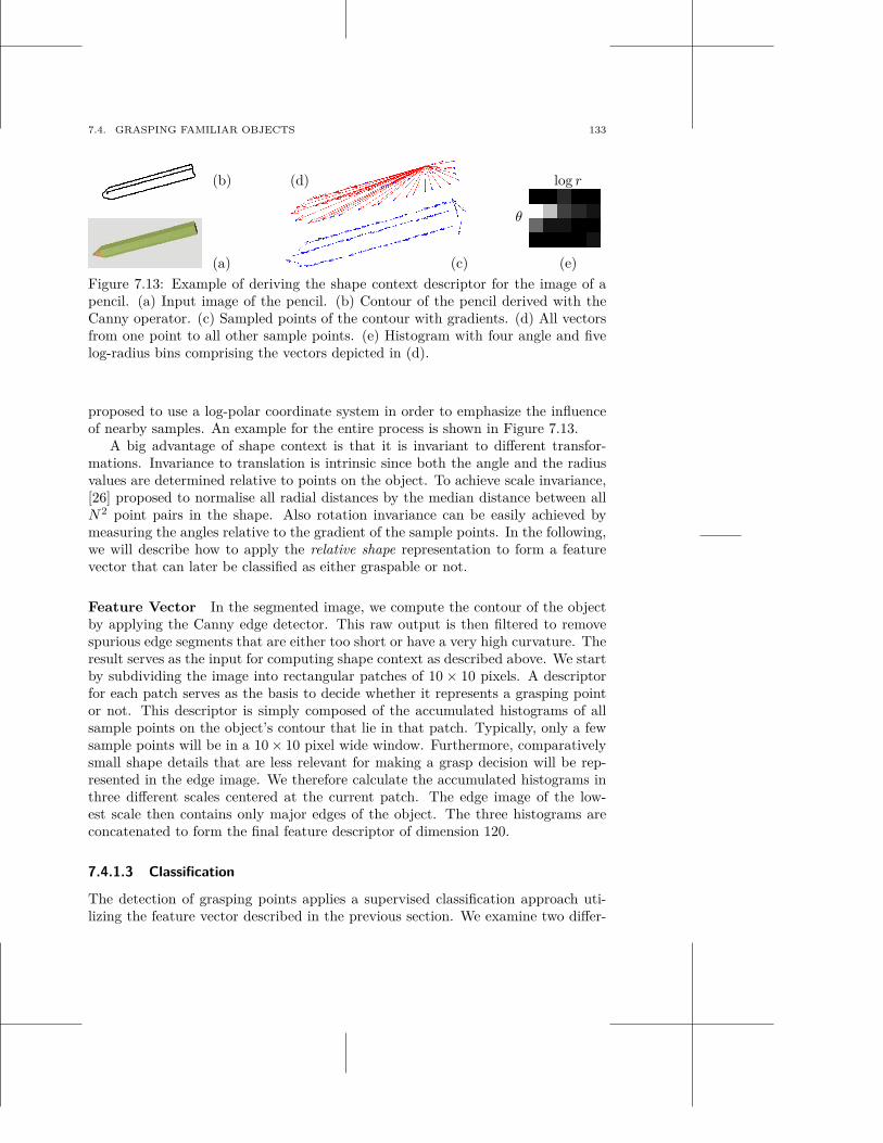
7.4. GRASPING FAMILIAR OBJECTS 133
(a)
(b)
(c)
(d) log r
θ
(e)
Figure 7.13: Example of deriving the shape context descriptor for the image of apencil. (a) Input image of the pencil. (b) Contour of the pencil derived with theCanny operator. (c) Sampled points of the contour with gradients. (d) All vectorsfrom one point to all other sample points. (e) Histogram with four angle and fivelog-radius bins comprising the vectors depicted in (d).
proposed to use a log-polar coordinate system in order to emphasize the influenceof nearby samples. An example for the entire process is shown in Figure 7.13.
A big advantage of shape context is that it is invariant to different transfor-mations. Invariance to translation is intrinsic since both the angle and the radiusvalues are determined relative to points on the object. To achieve scale invariance,[26] proposed to normalise all radial distances by the median distance between allN2 point pairs in the shape. Also rotation invariance can be easily achieved bymeasuring the angles relative to the gradient of the sample points. In the following,we will describe how to apply the relative shape representation to form a featurevector that can later be classified as either graspable or not.
Feature Vector In the segmented image, we compute the contour of the objectby applying the Canny edge detector. This raw output is then filtered to removespurious edge segments that are either too short or have a very high curvature. Theresult serves as the input for computing shape context as described above. We startby subdividing the image into rectangular patches of 10 × 10 pixels. A descriptorfor each patch serves as the basis to decide whether it represents a grasping pointor not. This descriptor is simply composed of the accumulated histograms of allsample points on the object’s contour that lie in that patch. Typically, only a fewsample points will be in a 10 × 10 pixel wide window. Furthermore, comparativelysmall shape details that are less relevant for making a grasp decision will be rep-resented in the edge image. We therefore calculate the accumulated histograms inthree different scales centered at the current patch. The edge image of the low-est scale then contains only major edges of the object. The three histograms areconcatenated to form the final feature descriptor of dimension 120.
7.4.1.3 Classification
The detection of grasping points applies a supervised classification approach uti-lizing the feature vector described in the previous section. We examine two differ-
134 CHAPTER 7. GENERATION OF GRASP HYPOTHESES
ent classification methods: a linear one (logistic regression) and a non-linear one(SVMs), [31]. We describe these briefly below.
Logistic Regression Let gi denote the binary variable for the ith image patchin the image. It can either carry the value 1 or 0 for being a grasping point ornot. The posterior probability for the former case will be denoted as p(gi = 1|fi)where fi is the feature descriptor of the ith image patch. For logistic regression, thisprobability is modelled as the sigmoid of a linear function of the feature descriptor:
p(gi = 1|fi) =1
1 + e−wfi(7.7)
where w is the weight vector of the linear model. These weights are estimated bymaximum likelihood:
w∗ = arg maxw′
∏
i
p(gi = 1|fi, w′) (7.8)
where here gi and fi are the labels and feature descriptors of our training data,respectively.
Support Vector Machines SVMs produce arbitrary decision functions in fea-ture space by a linear separation in a space of higher dimension compared to thefeature space. The mapping of the input data into that space is accomplished by anon-linear kernel function k. In order to obtain the model for the decision functionwhen applying SVMs, we solve the following optimisation problem:
max∑
i
αi − 12
∑
i,j
αiαjgigjk(fi, fj) (7.9)
subject to 0 ≤ αi ≤ C and∑
i αigi = 0 with the solution w =∑Ns
i αigifi. As akernel we have chosen a Radial Basis Function (RBF):
k(fi, fj) = e−γ||fi−fj ||2
, γ > 0 and γ =1
2σ2(7.10)
The two parameters C and σ are determined by a grid search over parameter space.In our implementation, we are using the package libsvm [50].
Training Database For training the different classifiers we will use the databasedeveloped by Saxena et al. [200] containing ca. 12000 synthetic images of eightobject classes depicted along with their grasp labels in Figure 7.14. One drawbackof the database is that the choice of grasping points is not always consistent withthe object category. As an example, a cup is labelled at two places on its rimbut all the points on the rim are equally well suited for grasping. The eraser isquite a symmetric object. Neither the local appearance nor the relative shape ofits grasping point are discriminative descriptors. This will be further discussed inSection 7.4.2 where our method is compared to that of [200].
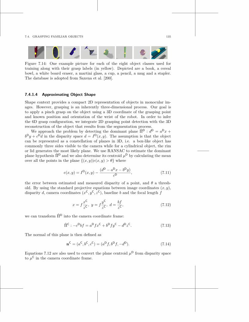
7.4. GRASPING FAMILIAR OBJECTS 135
Figure 7.14: One example picture for each of the eight object classes used fortraining along with their grasp labels (in yellow). Depicted are a book, a cerealbowl, a white board eraser, a martini glass, a cup, a pencil, a mug and a stapler.The database is adopted from Saxena et al. [200].
7.4.1.4 Approximating Object Shape
Shape context provides a compact 2D representation of objects in monocular im-ages. However, grasping is an inherently three-dimensional process. Our goal isto apply a pinch grasp on the object using a 3D coordinate of the grasping pointand known position and orientation of the wrist of the robot. In order to inferthe 6D grasp configuration, we integrate 2D grasping point detection with the 3Dreconstruction of the object that results from the segmentation process.
We approach the problem by detecting the dominant plane ΠD : dD = aDx +bDy + cDd in the disparity space d = ID(x, y). The assumption is that the objectcan be represented as a constellation of planes in 3D, i.e. a box-like object hascommonly three sides visible to the camera while for a cylindrical object, the rimor lid generates the most likely plane. We use RANSAC to estimate the dominantplane hypothesis ΠD and we also determine its centroid µD by calculating the meanover all the points in the plane {(x, y)|e(x, y) > θ} where
e(x, y) = ID(x, y) − (dD − aDx − bDy)cD
, (7.11)
the error between estimated and measured disparity of a point, and θ a thresh-old. By using the standard projective equations between image coordinates (x, y),disparity d, camera coordinates (xC, yC, zC), baseline b and the focal length f
x = fxC
zC, y = f
yC
zC, d =
bf
zC, (7.12)
we can transform ΠD into the camera coordinate frame:
ΠC : −cDbf = aDfxC + bDfyC − dDzC. (7.13)
The normal of this plane is then defined as
nC = (aC, bC, cC) = (aDf, bDf, −dD). (7.14)
Equations 7.12 are also used to convert the plane centroid µD from disparity spaceto µC in the camera coordinate frame.
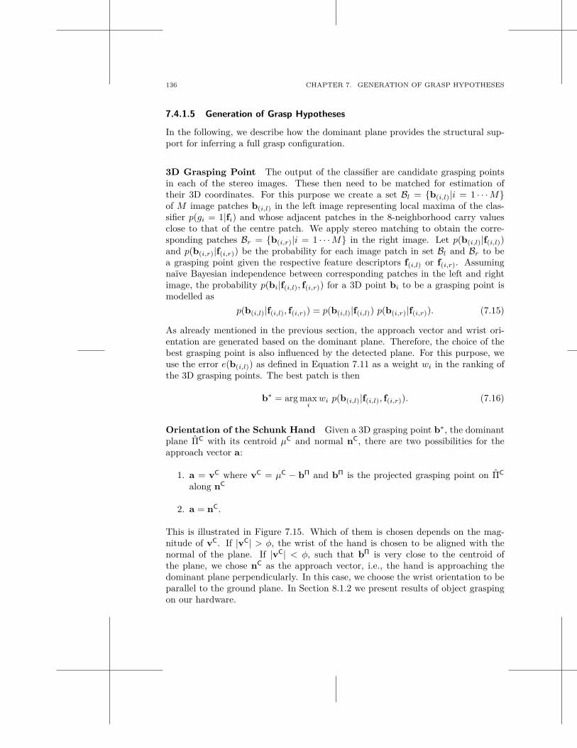
136 CHAPTER 7. GENERATION OF GRASP HYPOTHESES
7.4.1.5 Generation of Grasp Hypotheses
In the following, we describe how the dominant plane provides the structural sup-port for inferring a full grasp configuration.
3D Grasping Point The output of the classifier are candidate grasping pointsin each of the stereo images. These then need to be matched for estimation oftheir 3D coordinates. For this purpose we create a set Bl = {b(i,l)|i = 1 · · · M}of M image patches b(i,l) in the left image representing local maxima of the clas-sifier p(gi = 1|fi) and whose adjacent patches in the 8-neighborhood carry valuesclose to that of the centre patch. We apply stereo matching to obtain the corre-sponding patches Br = {b(i,r)|i = 1 · · · M} in the right image. Let p(b(i,l)|f(i,l))and p(b(i,r)|f(i,r)) be the probability for each image patch in set Bl and Br to bea grasping point given the respective feature descriptors f(i,l) or f(i,r). Assumingnaïve Bayesian independence between corresponding patches in the left and rightimage, the probability p(bi|f(i,l), f(i,r)) for a 3D point bi to be a grasping point ismodelled as
p(b(i,l)|f(i,l), f(i,r)) = p(b(i,l)|f(i,l)) p(b(i,r)|f(i,r)). (7.15)
As already mentioned in the previous section, the approach vector and wrist ori-entation are generated based on the dominant plane. Therefore, the choice of thebest grasping point is also influenced by the detected plane. For this purpose, weuse the error e(b(i,l)) as defined in Equation 7.11 as a weight wi in the ranking ofthe 3D grasping points. The best patch is then
b∗ = arg maxi
wi p(b(i,l)|f(i,l), f(i,r)). (7.16)
Orientation of the Schunk Hand Given a 3D grasping point b∗, the dominantplane ΠC with its centroid µC and normal nC, there are two possibilities for theapproach vector a:
1. a = vC where vC = µC − bΠ and bΠ is the projected grasping point on ΠC
along nC
2. a = nC.
This is illustrated in Figure 7.15. Which of them is chosen depends on the mag-nitude of vC. If |vC| > φ, the wrist of the hand is chosen to be aligned with thenormal of the plane. If |vC| < φ, such that bΠ is very close to the centroid ofthe plane, we chose nC as the approach vector, i.e., the hand is approaching thedominant plane perpendicularly. In this case, we choose the wrist orientation to beparallel to the ground plane. In Section 8.1.2 we present results of object graspingon our hardware.
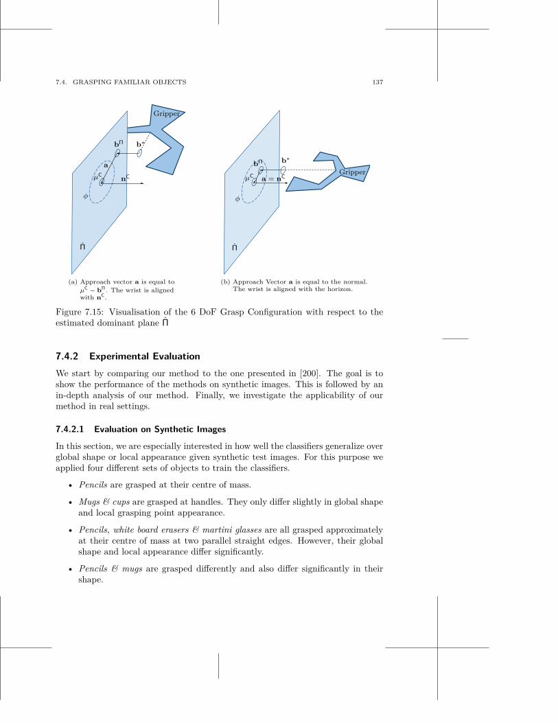
7.4. GRASPING FAMILIAR OBJECTS 137
Π
φ
µCnC
a
bΠ b∗
Gripper
(a) Approach vector a is equal to
µC − bΠ. The wrist is alignedwith nC.
Π
φ
µCa = nC
bΠ b∗
Gripper
(b) Approach Vector a is equal to the normal.The wrist is aligned with the horizon.
Figure 7.15: Visualisation of the 6 DoF Grasp Configuration with respect to theestimated dominant plane Π
7.4.2 Experimental Evaluation
We start by comparing our method to the one presented in [200]. The goal is toshow the performance of the methods on synthetic images. This is followed by anin-depth analysis of our method. Finally, we investigate the applicability of ourmethod in real settings.
7.4.2.1 Evaluation on Synthetic Images
In this section, we are especially interested in how well the classifiers generalize overglobal shape or local appearance given synthetic test images. For this purpose weapplied four different sets of objects to train the classifiers.
• Pencils are grasped at their centre of mass.
• Mugs & cups are grasped at handles. They only differ slightly in global shapeand local grasping point appearance.
• Pencils, white board erasers & martini glasses are all grasped approximatelyat their centre of mass at two parallel straight edges. However, their globalshape and local appearance differ significantly.
• Pencils & mugs are grasped differently and also differ significantly in theirshape.
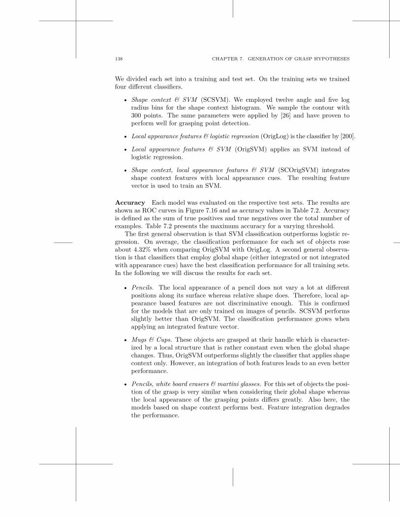
138 CHAPTER 7. GENERATION OF GRASP HYPOTHESES
We divided each set into a training and test set. On the training sets we trainedfour different classifiers.
• Shape context & SVM (SCSVM). We employed twelve angle and five logradius bins for the shape context histogram. We sample the contour with300 points. The same parameters were applied by [26] and have proven toperform well for grasping point detection.
• Local appearance features & logistic regression (OrigLog) is the classifier by [200].
• Local appearance features & SVM (OrigSVM) applies an SVM instead oflogistic regression.
• Shape context, local appearance features & SVM (SCOrigSVM) integratesshape context features with local appearance cues. The resulting featurevector is used to train an SVM.
Accuracy Each model was evaluated on the respective test sets. The results areshown as ROC curves in Figure 7.16 and as accuracy values in Table 7.2. Accuracyis defined as the sum of true positives and true negatives over the total number ofexamples. Table 7.2 presents the maximum accuracy for a varying threshold.
The first general observation is that SVM classification outperforms logistic re-gression. On average, the classification performance for each set of objects roseabout 4.32% when comparing OrigSVM with OrigLog. A second general observa-tion is that classifiers that employ global shape (either integrated or not integratedwith appearance cues) have the best classification performance for all training sets.In the following we will discuss the results for each set.
• Pencils. The local appearance of a pencil does not vary a lot at differentpositions along its surface whereas relative shape does. Therefore, local ap-pearance based features are not discriminative enough. This is confirmedfor the models that are only trained on images of pencils. SCSVM performsslightly better than OrigSVM. The classification performance grows whenapplying an integrated feature vector.
• Mugs & Cups. These objects are grasped at their handle which is character-ized by a local structure that is rather constant even when the global shapechanges. Thus, OrigSVM outperforms slightly the classifier that applies shapecontext only. However, an integration of both features leads to an even betterperformance.
• Pencils, white board erasers & martini glasses. For this set of objects the posi-tion of the grasp is very similar when considering their global shape whereasthe local appearance of the grasping points differs greatly. Also here, themodels based on shape context performs best. Feature integration degradesthe performance.

7.4. GRASPING FAMILIAR OBJECTS 139
• Pencils & mugs. The performance of the different classifiers for the previousset of objects is a first indication for a weaker generalization capability ofOrigSVM and OrigLog over varying local appearance compared to SCSVMand SCOrigSVM. This is further confirmed for the last set where not just localappearance but also global shape changes significantly. SCSVM improvesthe performance of OrigSVM about 6.75% even though the grasping pointsare very different when related to global object shape. Feature integrationincreases the performance only moderately.
Repeatability Our goal is to make a robot grasp arbitrary and novel objects.Thus, we are also interested in discovering whether the best grasping point hy-potheses correspond to points that in reality afford stable grasps. Thus, our secondexperiment evaluates whether the best hypotheses are located on or close to the la-belled points. We constructed a set of 80 images from the synthetic image databasewith ten randomly selected images of each of the eight object classes (Figure 7.14).Thus, also novel objects that were not used for training the different classifiers areconsidered. On every image we run all the aforementioned models and for each onepicked out the best ten grasping points bi. In the database, a label is not a singlepoint, but actually covers a certain area. We evaluated the Euclidean distance di
of each of the ten grasping points measured from the border of this ground truthlabel at position pj and normalized with respect to the length lj of its major axis.This way, the distance is dependent on the scale of the object in the image. In casethere is more than one label in the image, we choose the one with the minimumdistance. If a point bi lies directly on the label, the distance di = 0. If a pointlies outside of the label, the distance di gets weighted with a Gaussian function(σ = 1, µ = 0) multiplied with
√2π. The number of hits hm of each model m on
the picture set is counted as follows:
hm =K
∑
k=1
Nk∑
i=1
e−d2
(i,k)2
with d(i,k) =Mk
minj=1
dist(b(i,k), p(j,k))
2l(j,k)
where K is the number of images in the set, Mk is the number of grasp labels inthat picture and Nk is the number of detected grasping points. Grasping pointswhose distance di exceed a value of 3 ∗ σ are considered as outliers. Figure 7.17shows the number of hits, that is, the amount of good grasps for each model.
Apart from the model trained on cups and mugs, the SVM trained only onshape context always performs best. The performance drop for the second objectset can be explained in the same way as in the previous chapter: handles have avery distinctive local appearance and are therefore easily detected with features thatcapture this. In general, this result indicates that classifiers based on shape contextdetect grasping points with a better repeatability. This is particularly important
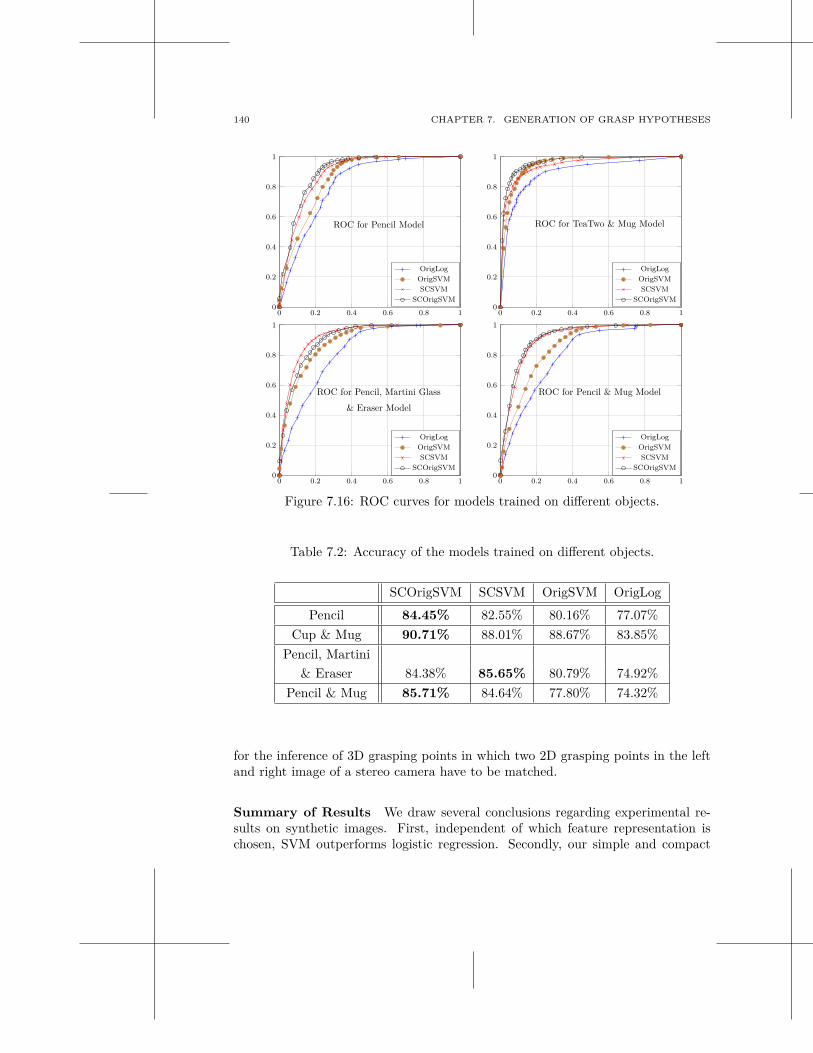
140 CHAPTER 7. GENERATION OF GRASP HYPOTHESES
0 0.2 0.4 0.6 0.8 10
0.2
0.4
0.6
0.8
1
OrigLog
OrigSVM
SCSVM
SCOrigSVM
ROC for Pencil Model
0 0.2 0.4 0.6 0.8 10
0.2
0.4
0.6
0.8
1
OrigLog
OrigSVM
SCSVM
SCOrigSVM
ROC for TeaTwo & Mug Model
0 0.2 0.4 0.6 0.8 10
0.2
0.4
0.6
0.8
1
OrigLog
OrigSVM
SCSVM
SCOrigSVM
ROC for Pencil, Martini Glass
& Eraser Model
0 0.2 0.4 0.6 0.8 10
0.2
0.4
0.6
0.8
1
OrigLog
OrigSVM
SCSVM
SCOrigSVM
ROC for Pencil & Mug Model
Figure 7.16: ROC curves for models trained on different objects.
Table 7.2: Accuracy of the models trained on different objects.
SCOrigSVM SCSVM OrigSVM OrigLog
Pencil 84.45% 82.55% 80.16% 77.07%
Cup & Mug 90.71% 88.01% 88.67% 83.85%
Pencil, Martini
& Eraser 84.38% 85.65% 80.79% 74.92%
Pencil & Mug 85.71% 84.64% 77.80% 74.32%
for the inference of 3D grasping points in which two 2D grasping points in the leftand right image of a stereo camera have to be matched.
Summary of Results We draw several conclusions regarding experimental re-sults on synthetic images. First, independent of which feature representation ischosen, SVM outperforms logistic regression. Secondly, our simple and compact
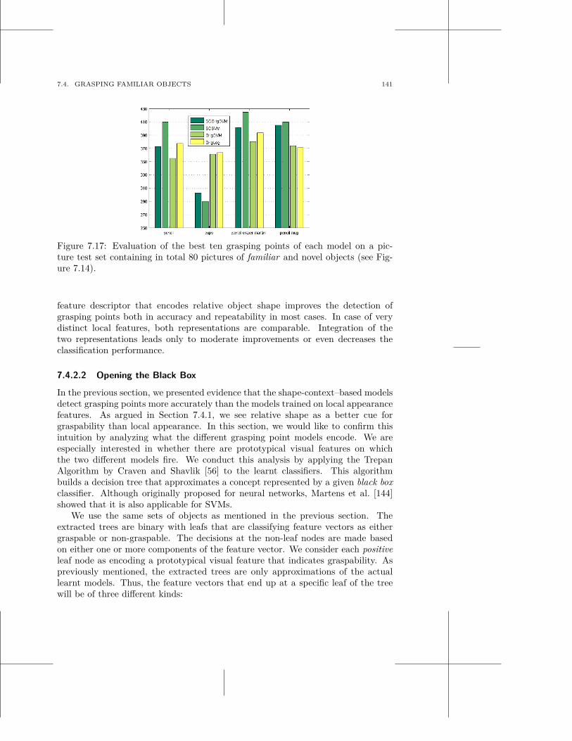
7.4. GRASPING FAMILIAR OBJECTS 141
Figure 7.17: Evaluation of the best ten grasping points of each model on a pic-ture test set containing in total 80 pictures of familiar and novel objects (see Fig-ure 7.14).
feature descriptor that encodes relative object shape improves the detection ofgrasping points both in accuracy and repeatability in most cases. In case of verydistinct local features, both representations are comparable. Integration of thetwo representations leads only to moderate improvements or even decreases theclassification performance.
7.4.2.2 Opening the Black Box
In the previous section, we presented evidence that the shape-context–based modelsdetect grasping points more accurately than the models trained on local appearancefeatures. As argued in Section 7.4.1, we see relative shape as a better cue forgraspability than local appearance. In this section, we would like to confirm thisintuition by analyzing what the different grasping point models encode. We areespecially interested in whether there are prototypical visual features on whichthe two different models fire. We conduct this analysis by applying the TrepanAlgorithm by Craven and Shavlik [56] to the learnt classifiers. This algorithmbuilds a decision tree that approximates a concept represented by a given black boxclassifier. Although originally proposed for neural networks, Martens et al. [144]showed that it is also applicable for SVMs.
We use the same sets of objects as mentioned in the previous section. Theextracted trees are binary with leafs that are classifying feature vectors as eithergraspable or non-graspable. The decisions at the non-leaf nodes are made basedon either one or more components of the feature vector. We consider each positiveleaf node as encoding a prototypical visual feature that indicates graspability. Aspreviously mentioned, the extracted trees are only approximations of the actuallearnt models. Thus, the feature vectors that end up at a specific leaf of the treewill be of three different kinds:
142 CHAPTER 7. GENERATION OF GRASP HYPOTHESES
• Ground truth. Features that are graspable according to the ground truthlabels in the database.
• False positives by model. Features that are not graspable according to thelabels but are so according to the classifier.
• False positives by tree. Features that are neither labelled in the database norclassified by the model to be graspable, but are considered to be so by thetree.
We will analyse these samples separately and also rate the trees by stating theirfidelity and accuracy. Fidelity is a measure of how well the extracted trees ap-proximate the considered models. It states the amount of feature vectors whoseclassification is compliant with the classification of the approximated model. Accu-racy measures the classification rate for either the tree or the model when run ona test set.
The analysis of these samples is conducted using PCA. The resulting eigenvec-tors form an orthonormal basis with the first eigenvector representing the directionof the highest variance, the second one the direction with the second largest vari-ance, etc. In the following sections we visualise only those eigenvectors whose energyis above a certain threshold and at maximum ten of these. The energy ei of aneigenvector ei is defined as
ei =
∑ij=1 λj
∑kj=1 λj
(7.17)
where λj is the eigenvalues of eigenvector ej with K eigenvectors in total. As athreshold we use θ = 0.9.
The remainder of this section is structured as follows. In Section 7.4.2.2, wevisualise the prototypical features for the local appearance method by applyingPCA to the samples at positive nodes. In Section 7.4.2.2 we do the same for therelative shape-based representation.
Local Appearance Features Saxena et al. [200] applied a filter bank to 10×10pixel patches in three spatial scales. The filter bank contains edge, texture (Law’smasks) and color filters. In this section, we depict samples of these 10 × 10 pixelpatches in the largest scale. They are taken from every positive node of each treetrained for a specific object set. All feature vectors that end up at one of thesepositive nodes are used as an input to PCA.
The first set we present consists of images of a pencil (see Figure 7.14) labelledin its centre of mass. The built tree is rather shallow: it has only four leaf nodesof which one is positive. The decisions on the non-leaf nodes are made basedon the output of the texture filters only. Neither color nor edge information areconsidered. This means that this part of the feature vector is not necessary toachieve a classification performance of 75.41% (see Table 7.3). Ten random samplesfrom the positive node are shown in Figure 7.18(a)-(c) subdivided dependent on
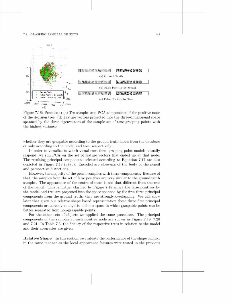
7.4. GRASPING FAMILIAR OBJECTS 143
(a) Ground Truth
(b) False Positive by Model
(c) False Positive by Tree
(d)
Figure 7.18: Pencils:(a)-(c) Ten samples and PCA components of the positive nodeof the decision tree. (d) Feature vectors projected into the three-dimensional spacespanned by the three eigenvectors of the sample set of true grasping points withthe highest variance.
whether they are graspable according to the ground truth labels from the databaseor only according to the model and tree, respectively.
In order to visualise to which visual cues these grasping point models actuallyrespond, we run PCA on the set of feature vectors that ended up at that node.The resulting principal components selected according to Equation 7.17 are alsodepicted in Figure 7.18 (a)-(c). Encoded are close-ups of the body of the penciland perspective distortions.
However, the majority of the pencil complies with these components. Because ofthat, the samples from the set of false positives are very similar to the ground truthsamples. The appearance of the centre of mass is not that different from the restof the pencil. This is further clarified by Figure 7.18 where the false positives bythe model and tree are projected into the space spanned by the first three principalcomponents from the ground truth: they are strongly overlapping. We will showlater that given our relative shape based representation these three first principalcomponents are already enough to define a space in which graspable points can bebetter separated from non-graspable points.
For the other sets of objects we applied the same procedure. The principalcomponents of the samples at each positive node are shown in Figure 7.19, 7.20and 7.21. In Table 7.3, the fidelity of the respective trees in relation to the modeland their accuracies are given.
Relative Shape In this section we evaluate the performance of the shape contextin the same manner as the local appearance features were tested in the previous
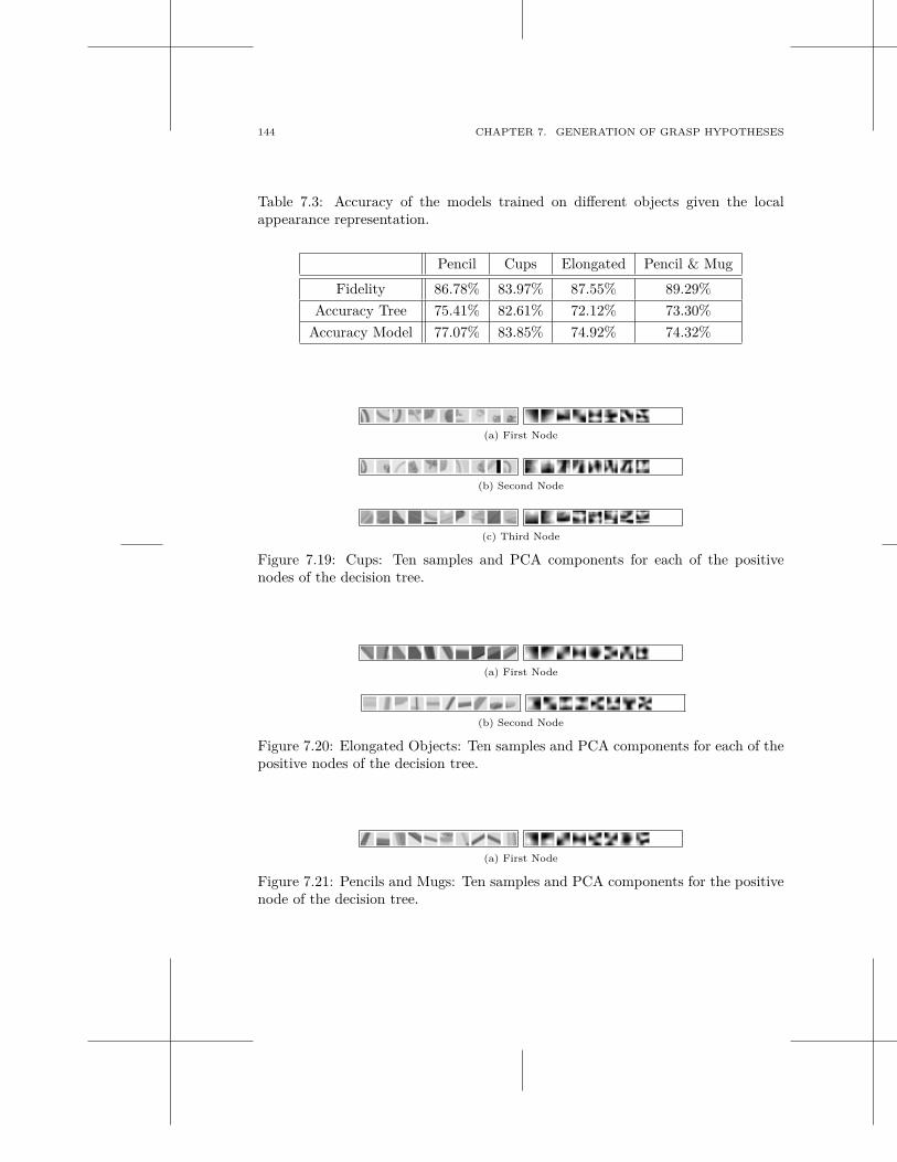
144 CHAPTER 7. GENERATION OF GRASP HYPOTHESES
Table 7.3: Accuracy of the models trained on different objects given the localappearance representation.
Pencil Cups Elongated Pencil & Mug
Fidelity 86.78% 83.97% 87.55% 89.29%
Accuracy Tree 75.41% 82.61% 72.12% 73.30%
Accuracy Model 77.07% 83.85% 74.92% 74.32%
(a) First Node
(b) Second Node
(c) Third Node
Figure 7.19: Cups: Ten samples and PCA components for each of the positivenodes of the decision tree.
(a) First Node
(b) Second Node
Figure 7.20: Elongated Objects: Ten samples and PCA components for each of thepositive nodes of the decision tree.
(a) First Node
Figure 7.21: Pencils and Mugs: Ten samples and PCA components for the positivenode of the decision tree.
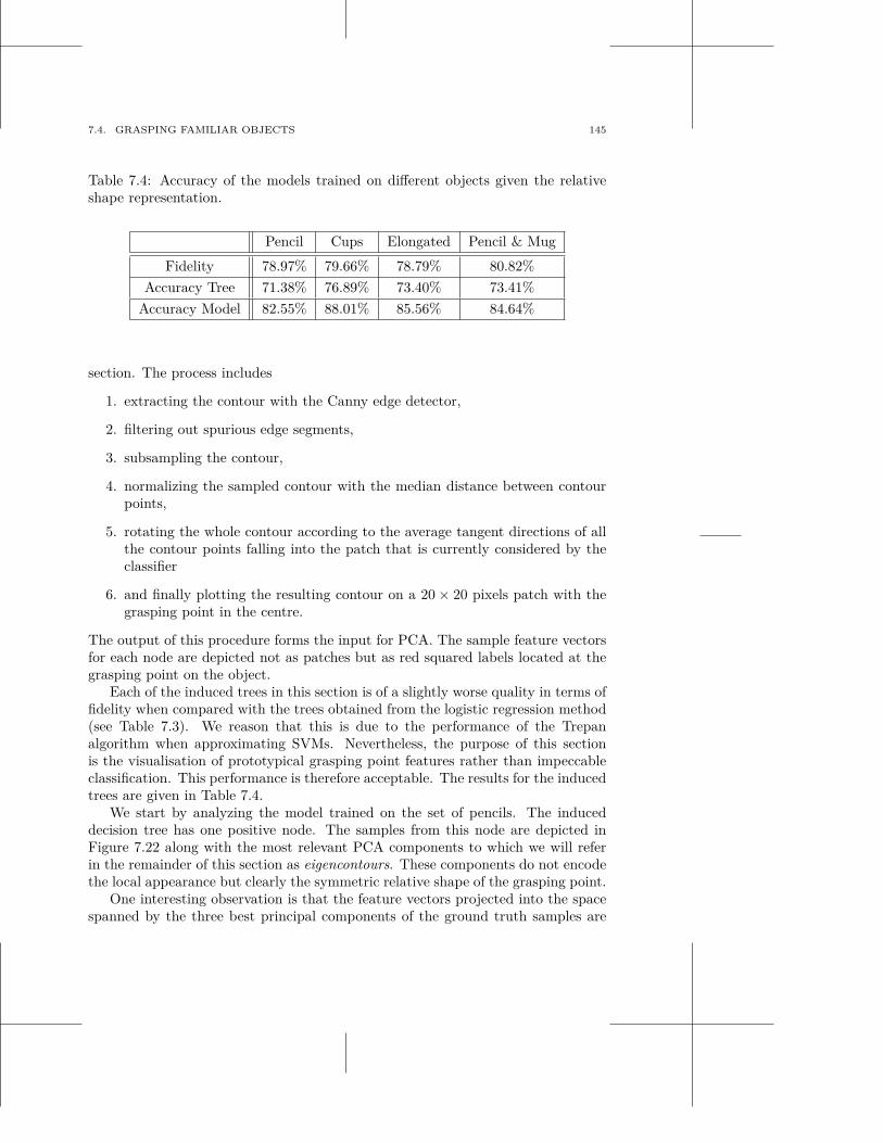
7.4. GRASPING FAMILIAR OBJECTS 145
Table 7.4: Accuracy of the models trained on different objects given the relativeshape representation.
Pencil Cups Elongated Pencil & Mug
Fidelity 78.97% 79.66% 78.79% 80.82%
Accuracy Tree 71.38% 76.89% 73.40% 73.41%
Accuracy Model 82.55% 88.01% 85.56% 84.64%
section. The process includes
1. extracting the contour with the Canny edge detector,
2. filtering out spurious edge segments,
3. subsampling the contour,
4. normalizing the sampled contour with the median distance between contourpoints,
5. rotating the whole contour according to the average tangent directions of allthe contour points falling into the patch that is currently considered by theclassifier
6. and finally plotting the resulting contour on a 20 × 20 pixels patch with thegrasping point in the centre.
The output of this procedure forms the input for PCA. The sample feature vectorsfor each node are depicted not as patches but as red squared labels located at thegrasping point on the object.
Each of the induced trees in this section is of a slightly worse quality in terms offidelity when compared with the trees obtained from the logistic regression method(see Table 7.3). We reason that this is due to the performance of the Trepanalgorithm when approximating SVMs. Nevertheless, the purpose of this sectionis the visualisation of prototypical grasping point features rather than impeccableclassification. This performance is therefore acceptable. The results for the inducedtrees are given in Table 7.4.
We start by analyzing the model trained on the set of pencils. The induceddecision tree has one positive node. The samples from this node are depicted inFigure 7.22 along with the most relevant PCA components to which we will referin the remainder of this section as eigencontours. These components do not encodethe local appearance but clearly the symmetric relative shape of the grasping point.
One interesting observation is that the feature vectors projected into the spacespanned by the three best principal components of the ground truth samples are
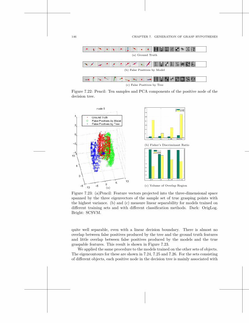
146 CHAPTER 7. GENERATION OF GRASP HYPOTHESES
(a) Ground Truth
(b) False Positives by Model
(c) False Positives by Tree
Figure 7.22: Pencil: Ten samples and PCA components of the positive node of thedecision tree.
(a)
(b) Fisher’s Discriminant Ratio
(c) Volume of Overlap Region
Figure 7.23: (a)Pencil: Feature vectors projected into the three-dimensional spacespanned by the three eigenvectors of the sample set of true grasping points withthe highest variance. (b) and (c) measure linear separability for models trained ondifferent training sets and with different classification methods. Dark: OrigLog.Bright: SCSVM.
quite well separable, even with a linear decision boundary. There is almost nooverlap between false positives produced by the tree and the ground truth featuresand little overlap between false positives produced by the models and the truegraspable features. This result is shown in Figure 7.23.
We applied the same procedure to the models trained on the other sets of objects.The eigencontours for these are shown in 7.24, 7.25 and 7.26. For the sets consistingof different objects, each positive node in the decision tree is mainly associated with
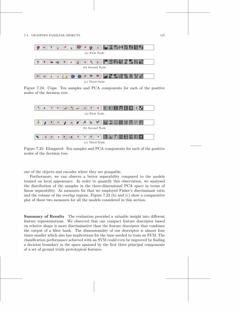
7.4. GRASPING FAMILIAR OBJECTS 147
(a) First Node
(b) Second Node
(c) Third Node
Figure 7.24: Cups: Ten samples and PCA components for each of the positivenodes of the decision tree.
(a) First Node
(b) Second Node
(c) Third Node
Figure 7.25: Elongated: Ten samples and PCA components for each of the positivenodes of the decision tree.
one of the objects and encodes where they are graspable.Furthermore, we can observe a better separability compared to the models
trained on local appearance. In order to quantify this observation, we analysedthe distribution of the samples in the three-dimensional PCA space in terms oflinear separability. As measures for that we employed Fisher’s discriminant ratioand the volume of the overlap regions. Figure 7.23 (b) and (c) show a comparativeplot of these two measures for all the models considered in this section.
Summary of Results The evaluation provided a valuable insight into differentfeature representations. We observed that our compact feature descriptor basedon relative shape is more discriminative than the feature descriptor that combinesthe output of a filter bank. The dimensionality of our descriptor is almost fourtimes smaller which also has implications for the time needed to train an SVM. Theclassification performance achieved with an SVM could even be improved by findinga decision boundary in the space spanned by the first three principal componentsof a set of ground truth prototypical features.
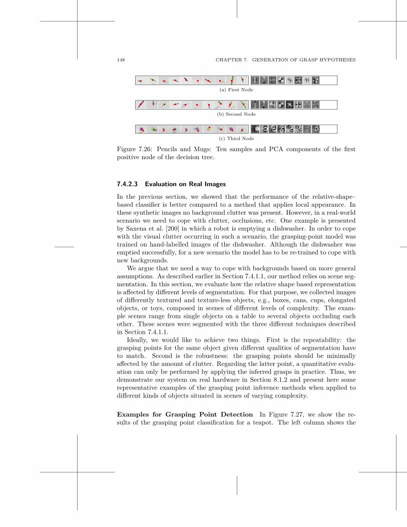
148 CHAPTER 7. GENERATION OF GRASP HYPOTHESES
(a) First Node
(b) Second Node
(c) Third Node
Figure 7.26: Pencils and Mugs: Ten samples and PCA components of the firstpositive node of the decision tree.
7.4.2.3 Evaluation on Real Images
In the previous section, we showed that the performance of the relative-shape–based classifier is better compared to a method that applies local appearance. Inthese synthetic images no background clutter was present. However, in a real-worldscenario we need to cope with clutter, occlusions, etc. One example is presentedby Saxena et al. [200] in which a robot is emptying a dishwasher. In order to copewith the visual clutter occurring in such a scenario, the grasping-point model wastrained on hand-labelled images of the dishwasher. Although the dishwasher wasemptied successfully, for a new scenario the model has to be re-trained to cope withnew backgrounds.
We argue that we need a way to cope with backgrounds based on more generalassumptions. As described earlier in Section 7.4.1.1, our method relies on scene seg-mentation. In this section, we evaluate how the relative shape based representationis affected by different levels of segmentation. For that purpose, we collected imagesof differently textured and texture-less objects, e.g., boxes, cans, cups, elongatedobjects, or toys, composed in scenes of different levels of complexity. The exam-ple scenes range from single objects on a table to several objects occluding eachother. These scenes were segmented with the three different techniques describedin Section 7.4.1.1.
Ideally, we would like to achieve two things. First is the repeatability: thegrasping points for the same object given different qualities of segmentation haveto match. Second is the robustness: the grasping points should be minimallyaffected by the amount of clutter. Regarding the latter point, a quantitative evalu-ation can only be performed by applying the inferred grasps in practice. Thus, wedemonstrate our system on real hardware in Section 8.1.2 and present here somerepresentative examples of the grasping point inference methods when applied todifferent kinds of objects situated in scenes of varying complexity.
Examples for Grasping Point Detection In Figure 7.27, we show the re-sults of the grasping point classification for a teapot. The left column shows the
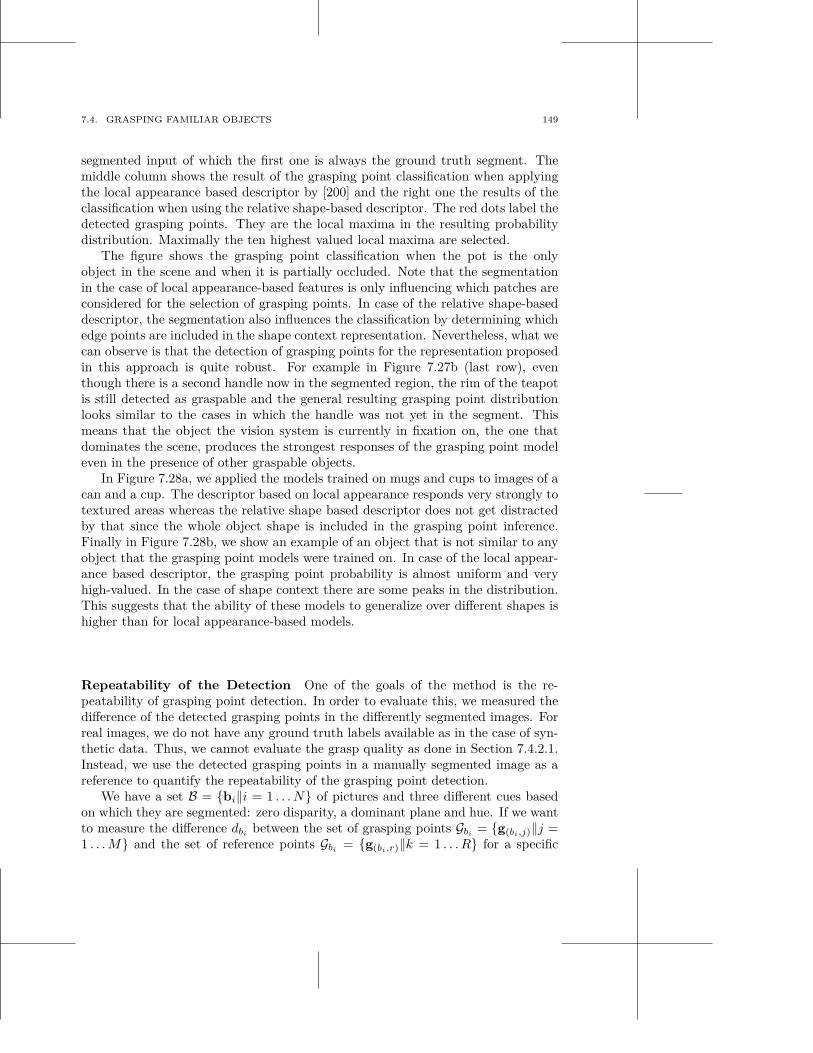
7.4. GRASPING FAMILIAR OBJECTS 149
segmented input of which the first one is always the ground truth segment. Themiddle column shows the result of the grasping point classification when applyingthe local appearance based descriptor by [200] and the right one the results of theclassification when using the relative shape-based descriptor. The red dots label thedetected grasping points. They are the local maxima in the resulting probabilitydistribution. Maximally the ten highest valued local maxima are selected.
The figure shows the grasping point classification when the pot is the onlyobject in the scene and when it is partially occluded. Note that the segmentationin the case of local appearance-based features is only influencing which patches areconsidered for the selection of grasping points. In case of the relative shape-baseddescriptor, the segmentation also influences the classification by determining whichedge points are included in the shape context representation. Nevertheless, what wecan observe is that the detection of grasping points for the representation proposedin this approach is quite robust. For example in Figure 7.27b (last row), eventhough there is a second handle now in the segmented region, the rim of the teapotis still detected as graspable and the general resulting grasping point distributionlooks similar to the cases in which the handle was not yet in the segment. Thismeans that the object the vision system is currently in fixation on, the one thatdominates the scene, produces the strongest responses of the grasping point modeleven in the presence of other graspable objects.
In Figure 7.28a, we applied the models trained on mugs and cups to images of acan and a cup. The descriptor based on local appearance responds very strongly totextured areas whereas the relative shape based descriptor does not get distractedby that since the whole object shape is included in the grasping point inference.Finally in Figure 7.28b, we show an example of an object that is not similar to anyobject that the grasping point models were trained on. In case of the local appear-ance based descriptor, the grasping point probability is almost uniform and veryhigh-valued. In the case of shape context there are some peaks in the distribution.This suggests that the ability of these models to generalize over different shapes ishigher than for local appearance-based models.
Repeatability of the Detection One of the goals of the method is the re-peatability of grasping point detection. In order to evaluate this, we measured thedifference of the detected grasping points in the differently segmented images. Forreal images, we do not have any ground truth labels available as in the case of syn-thetic data. Thus, we cannot evaluate the grasp quality as done in Section 7.4.2.1.Instead, we use the detected grasping points in a manually segmented image as areference to quantify the repeatability of the grasping point detection.
We have a set B = {bi‖i = 1 . . . N} of pictures and three different cues basedon which they are segmented: zero disparity, a dominant plane and hue. If we wantto measure the difference dbi
between the set of grasping points Gbi= {g(bi,j)‖j =
1 . . . M} and the set of reference points Gbi= {g(bi,r)‖k = 1 . . . R} for a specific
150 CHAPTER 7. GENERATION OF GRASP HYPOTHESES
kind of segmentation of the image bi, then
dbi=
1K
M∑
j=1
e−d2
j
2 where (7.18)
dj =R
minr=1
dist(g(bi,r), g(bi,j)) (7.19)
where dist is the Euclidean distance and K the length of the image diagonal3. Themean and standard deviation of dbi
for all images in the set B that are segmentedwith a specific cue is then our measure of deviation of the detected from the referencegrasping points.
In Figure 7.29 we show this measure for a representative selection of objectsand models. As already mentioned, ideally we would like to see no differencebetween detected grasping points when facing different qualities of segmentation.In practice, we can observe a flat slope. As expected for both methods, the graspingpoints detected in the image segmented with zero-disparity cues are the ones thatare deviating most from the reference points. Although, the selection of pointsthat are included in our representation is directly influenced by the segmentation,the difference between detected and reference grasping points is not always biggerthan for the appearance based method. In fact, sometimes it performs even better.This holds for examples of the models trained on mugs and cups for which bothmethods show a similar accuracy on synthetic data (Figure 7.29 (a) and (b)). Ifthe models are applied to novel objects, as can be observed in Figure 7.29 (c), ourdescriptors shows a better repeatability. This suggests again a better capabilityof the models to generalize across different relative shapes. In general, we can saythat both methods are comparable in terms of repeatability.
Summary of Results In this section, we evaluated the performance of our ap-proach on real images. Due to the encoding of global shape, the method is robustagainst occlusions and strong texture. Although our representation is strongly de-pendent on the segmentation, we observe that the repeatability of grasping pointsis comparable to the local appearance based method even when facing imperfectsegmentation. The analysis included images of varying qualities of segmentation aswell as occlusion and clutter.
7.5 Discussion
In this chapter, we reviewed approaches towards generating grasp hypotheses givendifferent kinds of prior object knowledge. Our proposed taxonomy is inspired byresearch in neuropsychology and classifies them dependent on whether they assume
3In our case K = 80 since we are evaluating 10 × 10 pixel patches in images of size 640 × 480pixels
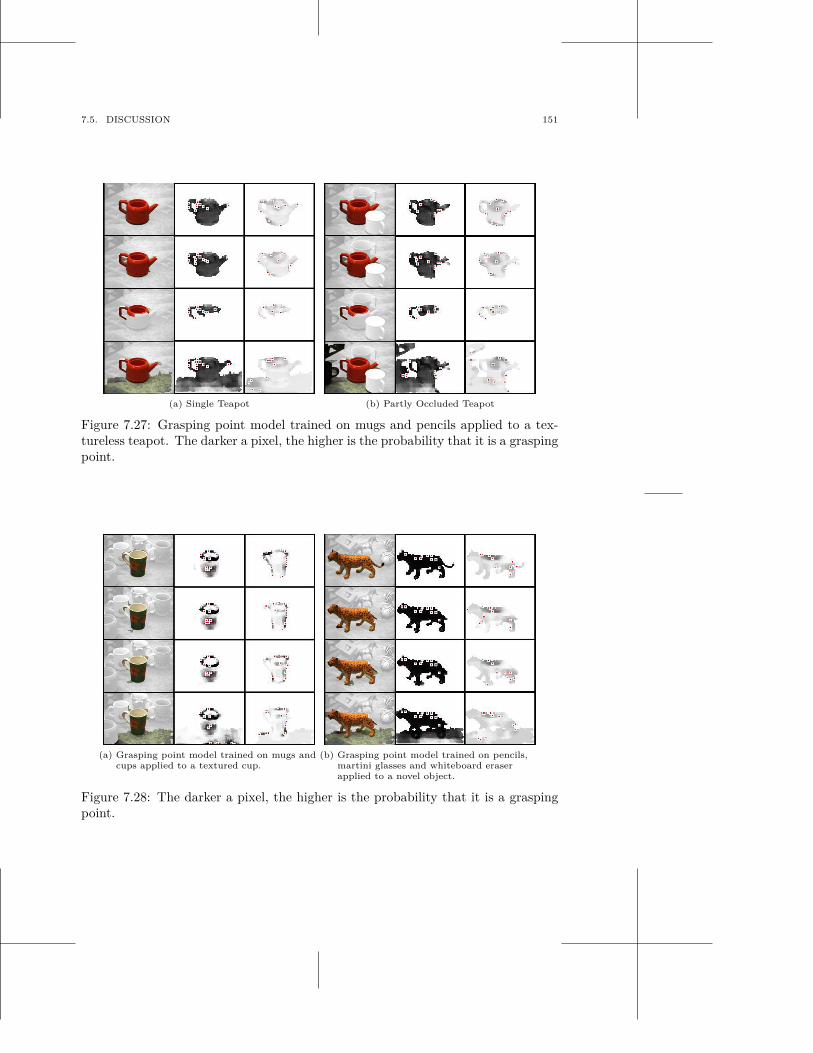
7.5. DISCUSSION 151
(a) Single Teapot (b) Partly Occluded Teapot
Figure 7.27: Grasping point model trained on mugs and pencils applied to a tex-tureless teapot. The darker a pixel, the higher is the probability that it is a graspingpoint.
(a) Grasping point model trained on mugs andcups applied to a textured cup.
(b) Grasping point model trained on pencils,martini glasses and whiteboard eraserapplied to a novel object.
Figure 7.28: The darker a pixel, the higher is the probability that it is a graspingpoint.
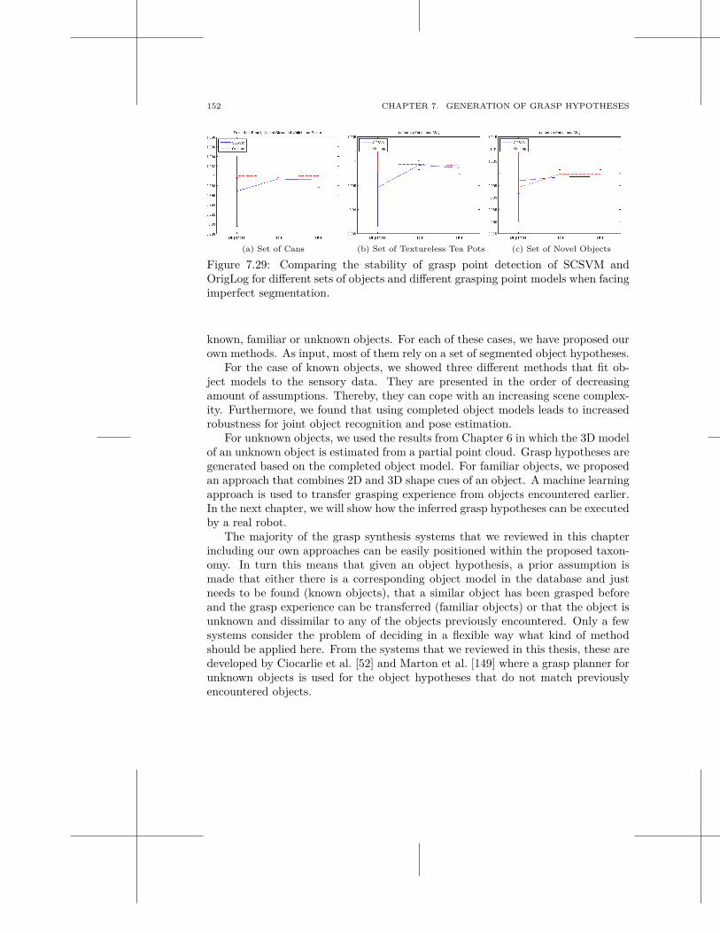
152 CHAPTER 7. GENERATION OF GRASP HYPOTHESES
(a) Set of Cans (b) Set of Textureless Tea Pots (c) Set of Novel Objects
Figure 7.29: Comparing the stability of grasp point detection of SCSVM andOrigLog for different sets of objects and different grasping point models when facingimperfect segmentation.
known, familiar or unknown objects. For each of these cases, we have proposed ourown methods. As input, most of them rely on a set of segmented object hypotheses.
For the case of known objects, we showed three different methods that fit ob-ject models to the sensory data. They are presented in the order of decreasingamount of assumptions. Thereby, they can cope with an increasing scene complex-ity. Furthermore, we found that using completed object models leads to increasedrobustness for joint object recognition and pose estimation.
For unknown objects, we used the results from Chapter 6 in which the 3D modelof an unknown object is estimated from a partial point cloud. Grasp hypotheses aregenerated based on the completed object model. For familiar objects, we proposedan approach that combines 2D and 3D shape cues of an object. A machine learningapproach is used to transfer grasping experience from objects encountered earlier.In the next chapter, we will show how the inferred grasp hypotheses can be executedby a real robot.
The majority of the grasp synthesis systems that we reviewed in this chapterincluding our own approaches can be easily positioned within the proposed taxon-omy. In turn this means that given an object hypothesis, a prior assumption ismade that either there is a corresponding object model in the database and justneeds to be found (known objects), that a similar object has been grasped beforeand the grasp experience can be transferred (familiar objects) or that the object isunknown and dissimilar to any of the objects previously encountered. Only a fewsystems consider the problem of deciding in a flexible way what kind of methodshould be applied here. From the systems that we reviewed in this thesis, these aredeveloped by Ciocarlie et al. [52] and Marton et al. [149] where a grasp planner forunknown objects is used for the object hypotheses that do not match previouslyencountered objects.
8
Grasp Execution
Many of the approaches that we reviewed in Section 7.1 for generating grasp hy-potheses are not demonstrated on a robot. For those who are, most of them employan open-loop controller. An open-loop controller computes its actions taking onlythe current state into account without observing the outcome of these actions andwhether they reached the desired goal.
However, realistic applications require going beyond open-loop execution to dealwith different types of errors occurring in an integrated robotic system. One kindof errors are systematic and repeatable, introduced mainly by inaccurate kinematicmodels. These can be minimized offline through precise calibration. The secondkind are random errors introduced by a limited repeatability of the motors orsensor noise. These have to be compensated online through for example closed-loop controllers. In a grasping system, this can be achieved through for examplevisual servoing or reactive grasping approaches using force-torque or tactile sensors.In these cases, the output of actions is observed during execution and actions areadapted to achieve the desired goal.
In this chapter, we will first demonstrate open-loop grasping given grasp hy-potheses from either familiar or unknown objects. This will serve as an example formotivating techniques for closed-loop execution of grasps. Different methods willbe reviewed. This will be followed by a demonstration of different visual servoingtechniques applied in our grasping pipeline for known and unknown objects.
8.1 Open Loop Grasp Execution
As an open-loop grasp controller, we consider a system that
• uses any of the grasp synthesis systems reviewed in the previous chapter tocompute a set of grasp hypotheses for an object,
• computes a trajectory to reach the desired grasp pose and
• executes this trajectory without any adaptation to, e.g., changes in the envi-ronment.
We employ such a controller to execute grasps for unknown and familiar objects.
153
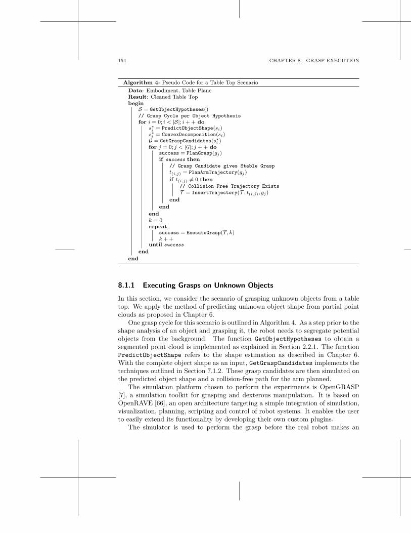
154 CHAPTER 8. GRASP EXECUTION
Algorithm 4: Pseudo Code for a Table Top Scenario
Data: Embodiment, Table PlaneResult: Cleaned Table Topbegin
S = GetObjectHypotheses()// Grasp Cycle per Object Hypothesis
for i = 0; i < |S|; i + + dos∗
i= PredictObjectShape(si)
s∗
i= ConvexDecomposition(si)
G = GetGraspCandidates(s∗
i)
for j = 0; j < |G|; j + + dosuccess = PlanGrasp(gj)if success then
// Grasp Candidate gives Stable Grasp
t(i,j) = PlanArmTrajectory(gj)
if t(i,j) 6= 0 then
// Collision-Free Trajectory Exists
T = InsertTrajectory(T , t(i,j), gj)
end
end
end
k = 0repeat
success = ExecuteGrasp(T, k)k + +
until success
end
end
8.1.1 Executing Grasps on Unknown Objects
In this section, we consider the scenario of grasping unknown objects from a tabletop. We apply the method of predicting unknown object shape from partial pointclouds as proposed in Chapter 6.
One grasp cycle for this scenario is outlined in Algorithm 4. As a step prior to theshape analysis of an object and grasping it, the robot needs to segregate potentialobjects from the background. The function GetObjectHypotheses to obtain asegmented point cloud is implemented as explained in Section 2.2.1. The functionPredictObjectShape refers to the shape estimation as described in Chapter 6.With the complete object shape as an input, GetGraspCandidates implements thetechniques outlined in Section 7.1.2. These grasp candidates are then simulated onthe predicted object shape and a collision-free path for the arm planned.
The simulation platform chosen to perform the experiments is OpenGRASP[7], a simulation toolkit for grasping and dexterous manipulation. It is based onOpenRAVE [66], an open architecture targeting a simple integration of simulation,visualization, planning, scripting and control of robot systems. It enables the userto easily extend its functionality by developing their own custom plugins.
The simulator is used to perform the grasp before the real robot makes an
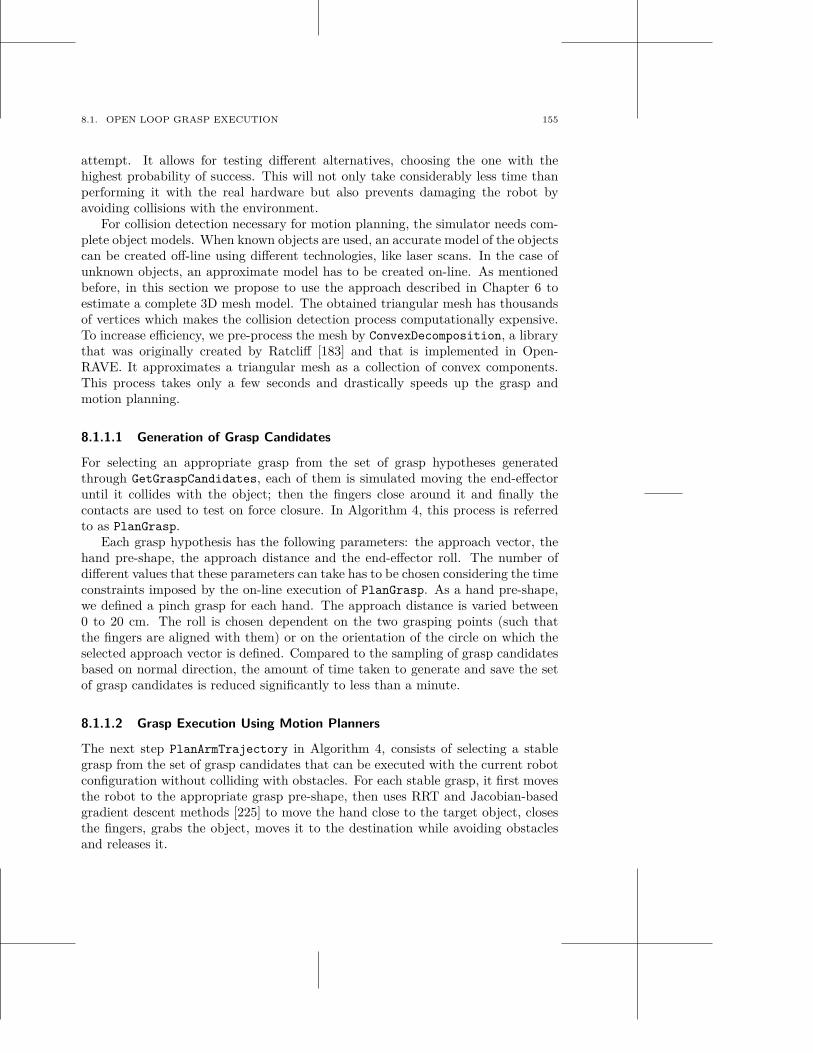
8.1. OPEN LOOP GRASP EXECUTION 155
attempt. It allows for testing different alternatives, choosing the one with thehighest probability of success. This will not only take considerably less time thanperforming it with the real hardware but also prevents damaging the robot byavoiding collisions with the environment.
For collision detection necessary for motion planning, the simulator needs com-plete object models. When known objects are used, an accurate model of the objectscan be created off-line using different technologies, like laser scans. In the case ofunknown objects, an approximate model has to be created on-line. As mentionedbefore, in this section we propose to use the approach described in Chapter 6 toestimate a complete 3D mesh model. The obtained triangular mesh has thousandsof vertices which makes the collision detection process computationally expensive.To increase efficiency, we pre-process the mesh by ConvexDecomposition, a librarythat was originally created by Ratcliff [183] and that is implemented in Open-RAVE. It approximates a triangular mesh as a collection of convex components.This process takes only a few seconds and drastically speeds up the grasp andmotion planning.
8.1.1.1 Generation of Grasp Candidates
For selecting an appropriate grasp from the set of grasp hypotheses generatedthrough GetGraspCandidates, each of them is simulated moving the end-effectoruntil it collides with the object; then the fingers close around it and finally thecontacts are used to test on force closure. In Algorithm 4, this process is referredto as PlanGrasp.
Each grasp hypothesis has the following parameters: the approach vector, thehand pre-shape, the approach distance and the end-effector roll. The number ofdifferent values that these parameters can take has to be chosen considering the timeconstraints imposed by the on-line execution of PlanGrasp. As a hand pre-shape,we defined a pinch grasp for each hand. The approach distance is varied between0 to 20 cm. The roll is chosen dependent on the two grasping points (such thatthe fingers are aligned with them) or on the orientation of the circle on which theselected approach vector is defined. Compared to the sampling of grasp candidatesbased on normal direction, the amount of time taken to generate and save the setof grasp candidates is reduced significantly to less than a minute.
8.1.1.2 Grasp Execution Using Motion Planners
The next step PlanArmTrajectory in Algorithm 4, consists of selecting a stablegrasp from the set of grasp candidates that can be executed with the current robotconfiguration without colliding with obstacles. For each stable grasp, it first movesthe robot to the appropriate grasp pre-shape, then uses RRT and Jacobian-basedgradient descent methods [225] to move the hand close to the target object, closesthe fingers, grabs the object, moves it to the destination while avoiding obstaclesand releases it.
156 CHAPTER 8. GRASP EXECUTION
Figure 8.1: Example of the grasp performed by the simulated robot and the realone, using Top) KTH platform and Bottom) UJI platform.
If the robot successfully grabs the object and moves it to the destination, thestable grasp is returned for execution with the real robot. Otherwise, the nextstable grasp from the set is tried. Figure 8.1 shows snapshots of the grasp executionusing the simulator and our robot. This work has been done in collaboration withthe Universitat Jaume I (UJI). How this grasp cycle is implemented on the verydifferent UJI platform is detailed in [4]. An example for the execution is shown inFigure 8.1.
8.1.2 Executing Grasps on Familiar Objects
In Section 7.4, we proposed a method for generating grasp hypotheses on familiarobjects in which 2D and 3D shape cues of an object hypothesis were combined. Amachine learning approach was used to transfer grasping experience from objectsencountered previously. 2D grasping points detected in such a way were used tosearch for full grasp poses given a minimal 3D representation. Since no mesh modelwas built of the object, the simulator was not used for grasp and motion planning.Instead, we inferred one grasp hypothesis and directly executed it on the robot.In Figure 8.2, video snapshots from the robot grasping three different objects aregiven along with the segmented input image, inferred grasping point distribution
8.2. CLOSED-LOOP GRASP EXECUTION 157
and detected dominant plane 1. For this demonstration, we rejected grasping pointsfor which the approach vector would result in a collision with the table.
In general, we can observe that the generated grasp hypotheses are reasonableselections from the huge amount of potentially applicable grasps. Failed grasps aredue to the fact that there is no closed-loop control implemented either in terms ofvisual servoing or hand movements.Grasps also fail due to the slippage or collision.
8.2 Closed-Loop Grasp Execution
Different to an open-loop grasp controller, a closed-loop controller does not executethe desired trajectory without taking feedback into account. Instead, the outcome ofthe execution is monitored constantly and adapted to ensure that the desired goal isreached. Different closed-loop systems have been employed for executing grasping.Visual Servoing techniques are mainly used for controlling the reaching trajectory.Reactive-grasp controllers employ force-torque or haptic sensors to ensure that thegrasp is successful.
After outlining the error sources in our robotic system in more detail, we willreview existing approaches for closed-control in grasping. This is followed by ex-amples on how we use different visual servoing techniques to grasp known andunknown objects as described in our previous work [10].
8.2.1 Error Sources in Our Robotic System
The grasp cycle outlined in Algorithm 4 relies on the assumption that all the param-eters of the system are perfectly known. This includes e.g. internal and externalcamera parameters as well as the pose of the head, arm and hand in a globallyconsistent coordinate frame.
In reality, however, two different types of errors are inherent to the system.One contains the systematic errors that are repeatable and arise from inaccuratecalibration or inaccurate kinematic models. The other group comprises randomerrors originating from noise in the motor encoders or in the camera. These errorspropagate and deteriorate the relative alignment between hand and object.
The most reliable component in our system is the Kuka arm that has a repeata-bility of less than 0.03 mm [126].
Our stereo calibration method uses the arm as world reference frame and isdescribed in more detail in [10]. We achieve an average re-projection error of 0.1pixels. Since peripheral and foveal cameras of the active head are calibrated simul-taneously, we also get the transformation between them.
Additionally to the systematic error in the camera parameters, other effects suchas camera noise and specularities lead to random errors in the stereo matching.
1A number of videos can be downloaded from www.csc.kth.se\~bohg.
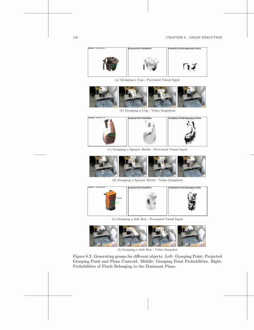
158 CHAPTER 8. GRASP EXECUTION
(a) Grasping a Cup - Processed Visual Input
(b) Grasping a Cup - Video Snapshots
(c) Grasping a Sprayer Bottle - Processed Visual Input
(d) Grasping a Sprayer Bottle - Video Snapshots
(e) Grasping a Salt Box - Processed Visual Input
(f) Grasping a Salt Box - Video Snapshot
Figure 8.2: Generating grasps for different objects: Left: Grasping Point, ProjectedGrasping Point and Plane Centroid. Middle: Grasping Point Probabilities. Right:Probabilities of Pixels Belonging to the Dominant Plane.
8.2. CLOSED-LOOP GRASP EXECUTION 159
Since we are using the arm to calibrate the stereo system, the error in thetransformation between the arm and cameras is proportional to the error of thestereo calibration.
We are using the robot head to actively explore the environment through gazeshifts and fixation on objects. This involves dynamically changing the epipolargeometry between the left and right camera system. Also the camera positionrelative to the head origin is changed. The internal parameters remain static. Onlythe last two joints of the head, the left and right eye yaw, are used for fixationand thereby affect the stereo calibration. The remaining joints are actuated forperforming gaze shifts.
In order to accurately detect objects with respect to the camera, the relationbetween the two camera systems as well as between the cameras and the headorigin needs to be determined after each movement. Ideally, these transformationsshould be obtainable just from the known kinematic chain of the robot and thereadings from the encoders. In reality, these readings are erroneous due to noiseand inaccuracies in the kinematic model. To reduce the systematic errors, we areextending our stereo calibration method to not just calibrate for one head pose,but for several. This is described in more detail in [10][13].
Regarding random error, the last five joints in the kinematic chain of the activehead achieve a repeatability in the range of ±0.025 degrees [17]. The neck pitchand neck roll joints have a lower repeatability in the range of ±0.13 and ±0.075degrees respectively.
8.2.2 Related Work
The systematic and random errors in the robotic system lead to an erroneous align-ment of the end effector with an object. A system that executes a grasp in an openloop fashion without taking any sensory feedback into account is likely to fail. Inthe following, we will review existing approaches towards calibrating the robot andtowards closed-loop control.
8.2.2.1 Calibration Methods
In [222], the authors presented a method for calibrating the active stereo head.The correct depth estimation of the system was demonstrated by letting it graspan object held in front of its eyes. No dense stereo reconstruction has been shownin this work.
Similarly, Welke et al. [229] present a procedure for calibrating the Karlsruherobotic head. Our calibration procedure [10] is similar to the one described in thosepapers, with a few differences. We extend it to the calibration of all joints, thusobtaining the whole kinematic chain. Also, the basic calibration method is modifiedto use an active pattern instead of a fixed checkerboard.
Pradeep et al. [173] present a system in which a robot moves a checkerboardpattern in front of its cameras to several different poses. Similar to our approach,
160 CHAPTER 8. GRASP EXECUTION
it can use its arms as kinematic chain sensors and automate the otherwise tediouscalibration process. However, the poses of the robot are hand crafted such thatthe checkerboard is guaranteed to be visible to the sensor that is to be calibrated.In our approach, we use visual servoing to automatically generate a calibrationpattern that is uniformly distributed in camera space.
8.2.2.2 Visual Servoing for Grasp Execution
Some grasping systems make use of visual feedback to correct the wrong alignmentbefore contact between the manipulator and the object is established. Examplesare proposed by Huebner et al. [102] and Ude et al. [223], who are using a similarrobotic platform to ours including an active head. In [102], the Armar III humanoidrobot is enabled to grasp and manipulate known objects in a kitchen environment.Similar to our system [13], a number of perceptual modules are at play to fulfillthis task. Attention is used for scene search. Objects are recognized and theirpose estimated with the approach originally proposed by Azad et al. [19]. Oncethe object identity is known, a suitable grasp configuration can be selected from anoffline constructed database. Visual servoing based on a spherical marker attachedto the wrist is applied to bring the robotic hand to the desired grasp positionas described in Vahrenkamp et al. [224]. Different from our approach, absolute3D data is estimated by fixing the 3 DoF for the eyes to a position for which astereo calibration exists. The remaining degrees of freedom controlling the neck ofthe head are used to keep the target and current hand position in view. In ourapproach, we reconstruct the 3D scene by keeping the eyes of the robot in constantfixation on the current object of interest. This ensures that the left and right visualfield overlap as much as possible, thereby maximizing e.g. the amount of 3D datathat can be reconstructed. However, the calibration process becomes much morecomplex.
In the work by Ude et al. [223], fixation plays an integral part of the visionsystem. Their goal is however somewhat different from ours. Given that an objecthas already been placed in the hand of the robot, it moves it in front of its eyesthrough closed-loop vision-based control. By doing this, it gathers several viewsfrom the currently unknown object for extracting a view-based representation thatis suitable for recognizing it later on. Different to our work, no absolute 3D in-formation is extracted for the purpose of object representation. Furthermore, theproblem of aligning the robotic hand with the object is circumvented.
8.2.2.3 Reactive Grasping Approaches
The main problem of open-loop grasping is that uncertainties introduced by theperception and motor systems are not taken into account during execution. Severalapproaches deal with this by either adapting the grasps online, by re-grasping orby taking uncertainties directly into account during learning appropriate grasps.
8.2. CLOSED-LOOP GRASP EXECUTION 161
In the following, we will review existing approaches divided regarding the assumedprior knowledge on the object.
Known Objects When the task of the robot is to grasp a known object, themain source of uncertainty lies in pose estimation. Bekiroglu et al. [25] use acombination of visual pose tracking and tactile features to assess grasp quality.The method is solved through supervised learning based on labeled training datato decide before lifting whether a grasp is going to be successful or not. Hsiaoet al. [100] approach the problem of grasping under pose uncertainty through adecision theoretic approach. Based on the current belief state, the system decidesbetween grasping and information-gathering actions using tactile input. Once theobject pose is known with sufficient certainty, grasping is executed. Tegin et al.[216] develop a reactive grasp controller in simulation in a framework of human-to-robot mapping of grasps. The approach is shown to be robust against pose errorsintroduced by visual pose estimation. Romero et al. [186] present a similar systembased on visual hand pose estimation instead of using a magnetic tracker. Notonly uncertainties in object pose but also inaccuracies in the mapping are takeninto account. Although the object is not explicitly modelled, it is assumed thatthe grasp to be imitated by the robot is performed on the same object in the samepose.
[124, 167] model the whole reaching and grasping movements. Pastor et al.[167] adjust movement primitives online to take pose uncertainties into account.Expected sensor readings during grasping an object are recorded from an idealdemonstration. During autonomous execution, the movement primitive is adaptedonline in case of divergences between the expected and actual sensor readings. Itis shown that this approach leads to an increased grasp success rate for differentobjects. As an open question remains how the system can select between a potentialset of object-specific expected sensors readings when executing a grasping action.
Kroemer et al. [124] apply a reinforcement learning approach in wich a low-levelreactive controller is applied to provide the high-level learner with rewards depen-dent on how much the fingers moved during the execution of the grasp. Primitivesmodeling the whole reaching movement are also adapted using a sparse visual rep-resentation of the environment to avoid collisions. This approach has been demon-strated for different objects in which the learnt policy converges to high rewardinggrasps.
Unknown Objects The challenge in the case of grasping unknown objects isdifferent from the previous case. Instead of an unknown relative pose betweenhand and object, here we have incomplete and noisy information about the objectgeometry. The following approaches assume that there is a system that providesthem with an initial grasp hypothesis. This can be any of those presented inSection 7.1.2. However, these hypotheses are usually inferred on either incompleteobject models or on completed but not necessarily accurate object models.
162 CHAPTER 8. GRASP EXECUTION
Felip and Morales [78] developed so called grasp primitives as indivisible actionsdefined by initial hand pre-shape, a sensor based controller and an end condition.The goal of these primitives is to achieve an alignment between object and handthat ensures a stable grasp. This is achieved by a sequence of re-grasping actions.Mainly, force-torque and finger joint readings are used. Hsiao et al. [99] proposea different reactive controller that uses contact information from tactile sensors.An adaption of the hand position dependent on the readings follows until contactwith the palm is detected and a compliant grasp is executed. Maldonado et al.[142] propose a similar approach using contact sensing in the fingertips duringthe approach of an object. Sensed obstacles are included in the representationof the environment and subsequently used to adapt the grasp hypothesis. Allthese approaches adapt the initial grasp hypothesis based on force-torque or tactilesensor readings. One of their disadvantages is that during contact the previousmodel of the scene might change. Previously inferred grasp hypothesis can thenbe inappropriate or even impossible. A new model of the world has to be acquiredwhich is an expensive operation.
A different reactive grasping approach is taken by Hsiao et al. [98] in whichoptical proximity sensors are used. Contact with the object is avoided while enoughinformation can be sensed to adapt the initial grasp strategy to something that hasa much higher likelihood to succeed.
8.2.3 Visual Servoing for Grasping Known Objects
In this section, we will demonstrate a simple position based visual servoing approachto perform grasping of known objects from a table top. We assume that the object tobe grasped has been segmented and reconstructed using the vision system describedin Section 2.2.1. Furthermore, we assume that the object has been recognized andits pose estimated using the approach described in Section 7.2.2.1. Due to the usageof a fixating system, we also know that the object is in the center of both, the leftand the right foveal camera.
From this information, we can infer all the parameters for a grasp. As approachvector we choose the negative gravity vector, i.e. in this scenario we will onlyperform simple top grasps. To determine the wrist orientation of the hand, we usethe information from pose estimation. In case of a roughly rectangular shape, theminor dimension is aligned with the vector between thumb and finger of the Schunkhand. For a circular shape, the wrist is left oriented in its default pose. As a fixedgrasping point, we choose the intersection between the principal axes of the left andright foveal camera in the arm base coordinate frame which we know to be lyingon the object.
8.2.3.1 Position-Based Visual Servoing for Alignment
In this scenario, we will use position-based visual servoing to align the hand with theobject prior to the actual grasp. The goal is to align the end effector in position xA
m
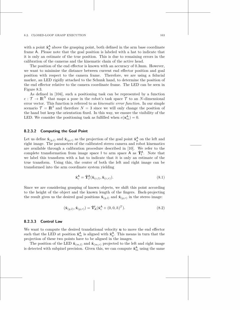
8.2. CLOSED-LOOP GRASP EXECUTION 163
with a point xAg above the grasping point, both defined in the arm base coordinate
frame A. Please note that the goal position is labeled with a hat to indicate thatit is only an estimate of the true position. This is due to remaining errors in thecalibration of the cameras and the kinematic chain of the active head.
The position of the end effector is known with an accuracy of 0.3mm. However,we want to minimise the distance between current end effector position and goalposition with respect to the camera frame. Therefore, we are using a fiducialmarker, an LED rigidly attached to the Schunk hand, to determine the position ofthe end effector relative to the camera coordinate frame. The LED can be seen inFigure 8.3.
As defined in [104], such a positioning task can be represented by a functione : T → IRN that maps a pose in the robot’s task space T to an N -dimensionalerror vector. This function is referred to as kinematic error function. In our simplescenario T = IR3 and therefore N = 3 since we will only change the position ofthe hand but keep the orientation fixed. In this way, we ensure the visibility of theLED. We consider the positioning task as fulfilled when e(xA
m) = 0.
8.2.3.2 Computing the Goal Point
Let us define x(g,l) and x(g,r) as the projection of the goal point xAg on the left and
right image. The parameters of the calibrated stereo camera and robot kinematicsare available through a calibration procedure described in [10]. We refer to thecomplete transformation from image space I to arm space A as TA
I. Note that
we label this transform with a hat to indicate that it is only an estimate of thetrue transform. Using this, the center of both the left and right image can betransformed into the arm coordinate system yielding
xA
c = TA
I (x(c,l), x(c,r)). (8.1)
Since we are considering grasping of known objects, we shift this point accordingto the height of the object and the known length of the fingers. Back-projectingthe result gives us the desired goal positions x(g,l) and x(g,r) in the stereo image:
(x(g,l), x(g,r)) = TI
A(xA
c + (0, 0, h)T ). (8.2)
8.2.3.3 Control Law
We want to compute the desired translational velocity u to move the end effectorsuch that the LED at position xA
m is aligned with xAg . This means in turn that the
projection of these two points have to be aligned in the images.The position of the LED x(m,l) and x(m,r) projected to the left and right image
is detected with subpixel precision. Given this, we can compute xAm using the same
164 CHAPTER 8. GRASP EXECUTION
transformation TA
I. Then the translational velocity is computed as
u = −k epp(xA
m; TA
I (x(g,l), x(g,r)), TA
I (x(m,l), x(m,r))) (8.3)
= −k epp(xA
m; xA
m, xA
g ) (8.4)
= −k (xA
m − xA
g ) (8.5)
where the argument left of the semicolon is the parameter to be controlled (theend effector position), and the arguments right after the semicolon parameterizethe positioning task. k is the gain parameter.
Once the robot hand is hovering over the object, we align the wrist correctlyand perform the actual grasp, lifting and transporting the object in an open-loopmanner. Example snapshots from a grasping action executed on the toy tiger isshown in Figure 8.3.
8.2.4 Virtual Visual Servoing for Grasping Unknown Objects
For the accurate control of the robotic manipulator using visual servoing, it isnecessary to know its position and orientation (pose) with respect to the camera.In the system exemplified in the previous section, the end effector of the robotsis tracked using an LED. These kind of fiducial markers are common solutions tothe tracking problem. In Section 8.2.2.2, we mentioned other approaches usingcolored spheres or Augmented Reality tags. A disadvantage of this marker-basedapproach is that the mobility of the robot arm is constrained to keep the markeralways in view. Furthermore, the position of the marker with respect to the endeffector has to be known exactly. For these reasons, we propose in [10] to trackthe whole manipulator instead of only a marker. Thereby, we alleviate the problemof constrained arm movement. Additionally, collisions with the object or otherobstacles can be avoided in a more precise way.
8.2.4.1 Image-Based Visual Servoing for Aligning the Virtual with the Real
Arm
Our approach to estimation and track the robot is based on virtual visual servoing(VVS) where a rendered model of a virtual robot is aligned with the current imageof their real counterparts. Figure 8.4 shows a comparison of the robot localisa-tion in the image using only calibration with the case when this localisation hasbeen corrected using VVS. In [10], this is achieved by extracting features from therendered image and compare them with the features extracted from the currentcamera image. Based on the extracted features, we define an error vector
s(t) = [d1, d2, . . . , dN ]T (8.6)
between the desired values for the features and the current ones. Let s be the rateof change of these distances given a change in pose of the end effector. This change
8.2. CLOSED-LOOP GRASP EXECUTION 165
(a) Positioning Arm Above Object. (b) Moving Arm Down to Pre-GraspPosition.
(c) Grasping the Object. (d) Lifting Object.
(e) Moving Object to Goal Position. (f) Release Object at Goal Position.
Figure 8.3: Example Grasp for the Recognized Tiger.
166 CHAPTER 8. GRASP EXECUTION
(a) (b)
Figure 8.4: Comparison of robot localization with (right) and without (left) theVirtual Visual Servoing correction.
can be described by a translational velocity t = [tx, ty, tz]T and a rotational velocityω = [ωx, ωy, ωz]T . Together, they form a velocity screw:
r(t) =[
tx, ty, tz, ωx, ωy, ωz
]T(8.7)
We can then define the image Jacobian as J so that:
s = Jr (8.8)
where
J =
[
∂s
∂r
]
=
∂d1
∂tx
∂d1
∂ty
∂d1
∂tz
∂d1
∂ωx
∂d1
∂ωy
∂d1
∂ωz
∂d2
∂tx
∂d2
∂ty
∂d2
∂tz
∂d2
∂ωx
∂d2
∂ωy
∂d2
∂ωz
......
......
......
∂dN
∂tx
∂dN
∂ty
∂dN
∂tz
∂dN
∂ωx
∂dN
∂ωy
∂dN
∂ωz
(8.9)
which relates the motion of the (virtual) manipulator to the variation in the features.Our goal however is to move the robot about r such that s becomes equal to 0.
Therefore, we need to compute r given s. In our case, the Jacobian is non-squareand therefore not invertible. Therefore, we compute
r = J+
s (8.10)
where J+ is the pseudoinverse of J .
Let us denote the pose of the virtual robot as TA, then the kinematic errorfunction eim can be defined as
eim(TA; s, 0) = 0 − s (8.11)
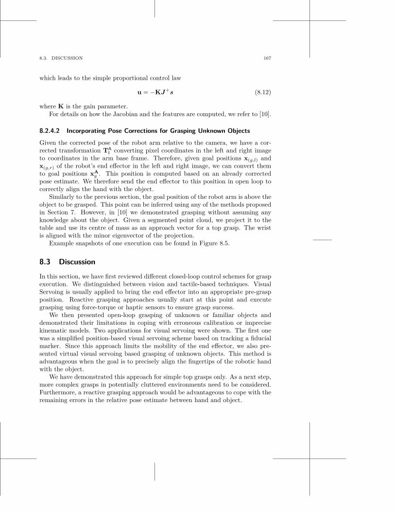
8.3. DISCUSSION 167
which leads to the simple proportional control law
u = −KJ+
s (8.12)
where K is the gain parameter.For details on how the Jacobian and the features are computed, we refer to [10].
8.2.4.2 Incorporating Pose Corrections for Grasping Unknown Objects
Given the corrected pose of the robot arm relative to the camera, we have a cor-rected transformation TA
Iconverting pixel coordinates in the left and right image
to coordinates in the arm base frame. Therefore, given goal positions x(g,l) andx(g,r) of the robot’s end effector in the left and right image, we can convert themto goal positions xA
g . This position is computed based on an already correctedpose estimate. We therefore send the end effector to this position in open loop tocorrectly align the hand with the object.
Similarly to the previous section, the goal position of the robot arm is above theobject to be grasped. This point can be inferred using any of the methods proposedin Section 7. However, in [10] we demonstrated grasping without assuming anyknowledge about the object. Given a segmented point cloud, we project it to thetable and use its centre of mass as an approach vector for a top grasp. The wristis aligned with the minor eigenvector of the projection.
Example snapshots of one execution can be found in Figure 8.5.
8.3 Discussion
In this section, we have first reviewed different closed-loop control schemes for graspexecution. We distinguished between vision and tactile-based techniques. VisualServoing is usually applied to bring the end effector into an appropriate pre-graspposition. Reactive grasping approaches usually start at this point and executegrasping using force-torque or haptic sensors to ensure grasp success.
We then presented open-loop grasping of unknown or familiar objects anddemonstrated their limitations in coping with erroneous calibration or imprecisekinematic models. Two applications for visual servoing were shown. The first onewas a simplified position-based visual servoing scheme based on tracking a fiducialmarker. Since this approach limits the mobility of the end effector, we also pre-sented virtual visual servoing based grasping of unknown objects. This method isadvantageous when the goal is to precisely align the fingertips of the robotic handwith the object.
We have demonstrated this approach for simple top grasps only. As a next step,more complex grasps in potentially cluttered environments need to be considered.Furthermore, a reactive grasping approach would be advantageous to cope with theremaining errors in the relative pose estimate between hand and object.
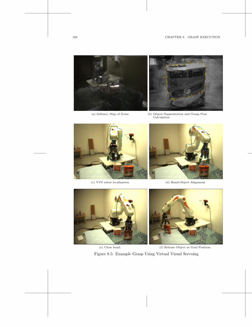
168 CHAPTER 8. GRASP EXECUTION
(a) Saliency Map of Scene (b) Object Segmentation and Grasp PoseCalculation
(c) VVS robot localization (d) Hand-Object Alignment
(e) Close hand. (f) Release Object at Goal Position.
Figure 8.5: Example Grasp Using Virtual Visual Servoing
9
Conclusions
A long-term goal in robotics research is to build an intelligent machine that canbe our companion in everyday life. It is thought to help us with tasks that arefor example difficult, dangerous or bothersome. However for many of these tasksthat we perform effortlessly, current robotic systems still lack the robustness andflexibility to carry them out equally well.
In this thesis, we considered a household scenario in which one of the key capa-bilities of a robot is grasping and manipulation of objects. Specifically, we focussedon the problem of scene understanding for object grasping. We followed the ap-proach of introducing prediction into the perceive-act loop. We showed how thishelps to efficiently explore a scene but also how it can be exploited to improvemanipulation.
We studied different scene representations as a container for knowledge aboutthe geometric structure of the environment. They are of varying complexity andutility, reaching from a classical occupancy grid map, over a height map to a 3Dpoint cloud. While the occupancy grid map allows to estimate free and occupiedspaces in the scene, a height map provides additional geometric information es-sential to manipulation. A point cloud can retain scene geometry most accuratelywhile not providing the efficiency of the other two approaches.
All these representations where studied considering fusion of multi-modal sen-sory data. Visual sensing through monocular and stereo cameras is the most im-portant modality used in this thesis. Haptic sensors provided information aboutareas in the scene that could not be visually observed. Furthermore, we used ob-ject recognition and pose estimation as a virtual sensor. Finally, we showed howinformation from a human operator enhances object segmentation.
In this thesis, prior knowledge about objectness or common scene structure wasexploited for predicting unexplored, unobserved or uncertain parts of the scene. InChapter 4, we used Gaussian Processes to predict scene geometry based on partsthat have already been observed. The prior knowledge is constituted of a kernelfunction that reflects common object shape. In Chapter 5, we made use of theobservation that objects are relatively homogenous in their attribute space. Thisprior helped the robot to autonomously evaluate segmentation quality. In Chap-ter 6, we proposed an approach for estimating the backside of unknown objects. It
169
170 CHAPTER 9. CONCLUSIONS
is based on the prior knowledge that man-made objects are commonly symmetric.Additionally to estimating the unobserved parts of the scene, we showed how
we can quantify the uncertainty about the prediction. This becomes useful forchoosing the most beneficial exploratory actions. In Chapter 4, these actions wereperformed with the robot hand equipped with haptic sensor matrices. In Chapter 5,a human was questioned to confirm whether an uncertain object hypothesis has tobe corrected or not.
Apart from selecting exploratory actions to refine a scene model, we have alsoshown how predictions can improve grasp synthesis. Dependent on whether theobjects are known, familiar or unknown, different methodologies for grasp inferenceapply. In Chapter 7, we reviewed related approaches according to this taxonomy.Foreach case, we proposed a novel method extending the state of the art. For knownobjects, we showed that using a completed point cloud is rendering pose estimationmore robust. For unknown objects, we showed how completed point cloud help toinfer more robust grasps. And finally for familiar objects, we showed that givenan accurate object segmentation, good grasp points can be inferred based on theobject’s global shape. We demonstrated these approaches in real-world scenes oftable-top scenarios thereby proving their feasibility.
In Section 1.1, we showed an example scenario in which a robot is asked toclean a very messy office desk. We listed several scientific challenges that have tobe solved before a real robot will be able to fulfill such a task satisfactorily. In thisthesis, we made contributions to the subtasks of scene understanding and roboticgrasping. Given different scene representations, sensors and prior knowledge, weproposed several prediction mechanisms that provide the robot with informationbeyond what is has directly observed.
However, many scientific challenges still remain before a robot can autonomouslyclean a desk as envisioned in the introduction of this thesis. In the following, wewill outline the parts that we believe have to be solved next.
Independence of Table-Top Detection Almost all of the proposed methodsfor scene understanding rely on knowing the dominant plane on which the objectswhere arranged. This allowed us to use efficient scene representations and a re-duction of the search space for object shape prediction. However, extracting thetable-top might not be trivial due to clutter. Hence, the proposed representationshave to be made independent of this knowledge while at the same time remain ef-ficiently computable. If the dominant plane can however be detected, the resultingpossibility to reduce the search space should be made use of.
Grasp-Oriented Active Perception Considering the tremendous amount ofmemory that would be required to store an accurate and detailed 3D point cloudof a large scale environment, we need to find a more efficient way to represent it.This representation has to retain the amount of information that makes it possiblefor the robot to roughly plan its course of actions. We believe, that the fine detail
171
information necessary for example for collision avoidance, opening doors or graspplanning, should be obtained rapidly and only on demand in the context of specificbehaviors and tasks.
Learning Priors In all chapters, we have used prior assumptions about scenestructure and objectness. This reaches from blob-like kernel functions over homo-geneity in specific object attributes to symmetric shape of objects. We showed thatthese priors are useful in predicting the structure of unknown space. While webelieve that it is adequate to make assumptions about some low-level priors, thequestions remains how additional priors can be learnt autonomously and adaptediteratively over a much longer time span (potentially life-long).
Transferring Affordances As has been shown in Chapter 7, there is quite alarge body of work on generating grasp hypotheses given an object hypothesis.One kind of these methods aims at transferring grasp experience from previouslyencountered objects to new ones. Many of these methods rely on relatively low-level features like distribution of edges, color or texture. Only very few make use ofhigher-level information like object identity or category. However, we believe thatonly given such information allows to link the generated grasp hypotheses to tasks.
Adaptation of Grasp Hypotheses The prediction mechanism that we pro-posed in this thesis have mainly been used to trigger exploratory actions. Thisin turn led to an improved scene model with correct object hypotheses. Howeveronly the result of the method proposed in Chapter 6 was used to improve grasp hy-pothesis selection. The robustness of grasping could be improved if the remaininguncertainty in the scene model is explicitly included in the grasp synthesis process.
Multi-Modal Closed-Loop Control In Chapter 8, we showed how Visual Ser-voing and Virtual Visual Servoing can help to improve grasp execution in a closed-loop fashion. However, these techniques were so far only used for aligning the robothand with the object. The actual grasping, i.e. closing the fingers around the objectand lifting it, were performed open loop only. To enable the robot to grasp objectsrobustly and adapt its behavior when facing unexpected sensor reading, we needto adopt a reactive grasping approach. This should not only involve haptic sensordata from tactile or force-torque sensors. It should also include visual tracking ofthe object that is manipulated. Furthermore, the uncertainty about the geometryof the object or the scene should influence execution of the grasp as well. It mightfor example influence grasp parameters such as pre-shape or velocity of the endeffector.

A
Covariance Functions
Throughout this thesis, we use different learning techniques to enable a robot toextrapolate from prior experience. For example in Chapter 4, the robot has topredict the geometry of a scene from partial visual observations. These observationscan be formally seen as a set of inputs X for which we already know the correcttarget values Y. For new inputs x′ that we do not yet know the appropriate targetvalue of, we use the concept of similarity. New inputs that are close to alreadyknown ones should have similar target values.
In the framework of Gaussian Processes, the similarity is defined through co-variance functions. In the following, we present the covariance functions used inChapter 4 in a bit more detail. Figure A.1 visualises these different functions. Fora more detailed review, we refer to [181].
Squared Exponential Covariance Function Most of the covariance functionspresented here are stationary. They are functions of the difference r = x − x′
between input points. These functions are therefore invariant to translations. Thesquared exponential covariance function (SE) is defined as
kSE(r) = exp(− r2
2l2). (A.1)
Dependent on the hyperparameter l, the length scale, this function places a moreor less strong smoothing on the input signal. It is visualized for different lengthscales in Figure A.1a.
Mátern Class of Covariance Functions The strong smoothing of the SE ker-nel has been argued to be unrealistic for most physical processes [181]. The Máternclass is more flexible and allows varying degrees of smoothness. It is dependenton the two parameters ν and l. In this thesis, we only looked at the case where νis a half-integer and the covariance function can be significantly simplified. Withν = 1/2, the covariance function is equal to the exponential function
kMat1(r) = exp(−r/l). (A.2)
173
174 APPENDIX A. COVARIANCE FUNCTIONS
We also tested the cases where ν = 3/2 and ν = 5/2 that are claimed by Bishop[31] to be the most interesting for machine learning applications:
kMat3(r) =(1 +
√3r
l) exp(−
√3r
l) (A.3)
kMat5(r) =(1 +
√5r
l+
5r2
3l2) exp(−
√5r
l). (A.4)
These cases of the Mátern class are visualized in Figures A.1b, A.1c and A.1d. Withν → ∞, the Mátern covariance function becomes the squared exponential function.
Rational Quadratic Covariance Function This covariance function is depen-dent on the two hyperparameter l and α. It is defined as
kRQ(r) = (1 +r2
2αl2)−α. (A.5)
Fixing the length scale l = 1, the RQ kernel is visualized for different α in Fig-ure A.1e. It can be seen as a scale mixture of SE kernels with different characteristiclength scales. With α → ∞ the RQ function becomes an SE function with lengthscale l.
SE with Automatic Relevance Detection Although the previous RQ kernelis flexible through a mixture of SE kernels of different length scales, it still valueseach input value in the set X as equally important. If the dimension of the inputspace D > 1, then the SE covariance function can also be written as
kSEARD(r) = σ2f exp(−1
2rT Mr) (A.6)
where M = diag(l)−2. The vector l is of dimension D. Each component equals thecharacteristic length scale of each dimension of the input space. Therefore, if one ofthe dimensions has a very large length scale, it will become irrelevant for inference.
Neural Network Covariance Function This covariance function is non-stationary,i.e., it is not invariant to translations. It is derived from a neural network architec-ture with N units that implement a specific hidden transfer function h(x; u) withu as input-to-hidden weights. It takes in an input x and combines the outputs ofthe units linearly with a bias to evaluate the function f(x). Setting the transferfunction h(x; u) = erf(u0 + ΣD
j=1ujxj), the covariance function is defined as follows
kNN (x, x′) =2π
arcsin(2xT Σx′
√
(1 + 2xT Σx)(1 + 2x′T Σx′)) (A.7)
where x = (1, x1, · · · , xD) is the augmented input vector. It is visualized in Fig-ure A.1f for Σ = diag(σ2
0 , σ2) with σ20 = σ2 = 10.
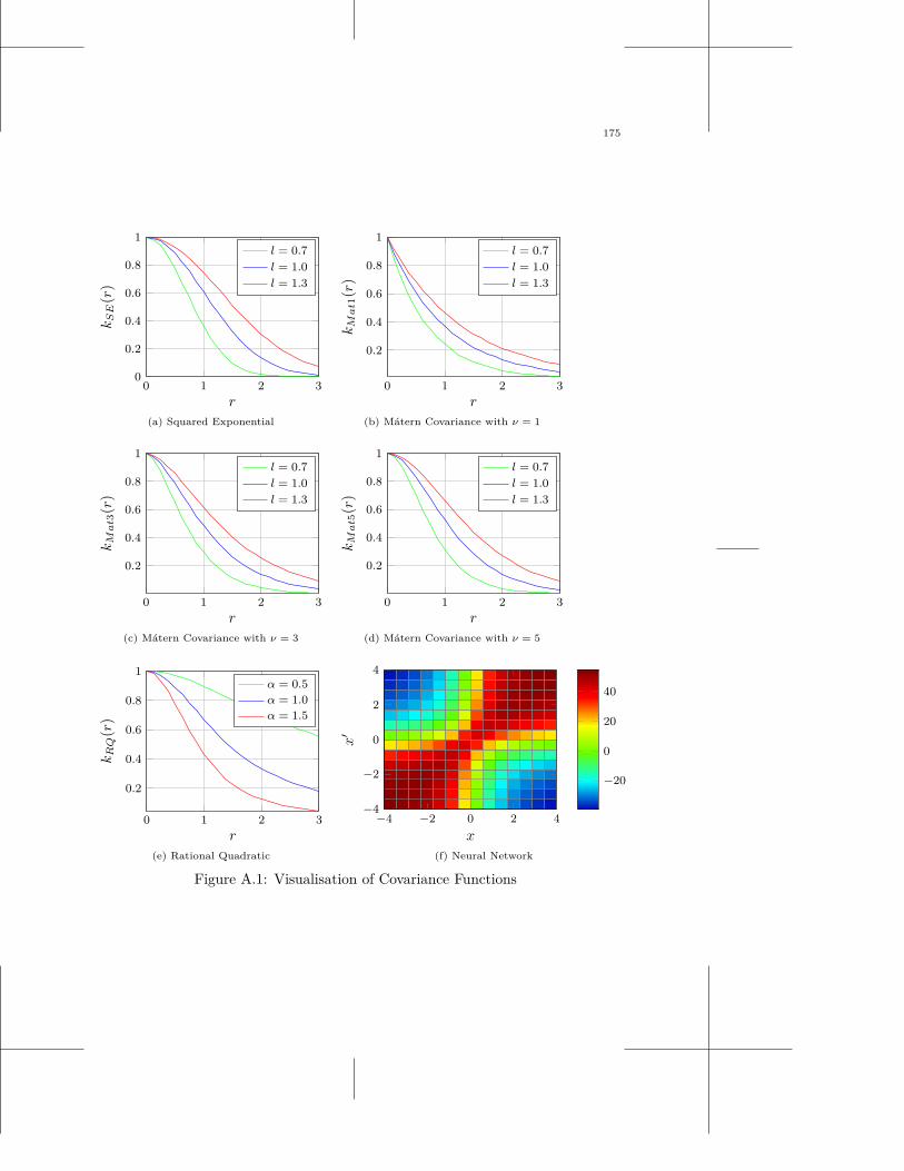
175
0 1 2 30
0.2
0.4
0.6
0.8
1
r
kS
E(r
)
l = 0.7
l = 1.0
l = 1.3
(a) Squared Exponential
0 1 2 3
0.2
0.4
0.6
0.8
1
r
kM
at1
(r)
l = 0.7
l = 1.0
l = 1.3
(b) Mátern Covariance with ν = 1
0 1 2 3
0.2
0.4
0.6
0.8
1
r
kM
at3
(r)
l = 0.7
l = 1.0
l = 1.3
(c) Mátern Covariance with ν = 3
0 1 2 3
0.2
0.4
0.6
0.8
1
r
kM
at5
(r)
l = 0.7
l = 1.0
l = 1.3
(d) Mátern Covariance with ν = 5
0 1 2 3
0.2
0.4
0.6
0.8
1
r
kR
Q(r
)
α = 0.5
α = 1.0
α = 1.5
(e) Rational Quadratic
−4 −2 0 2 4−4
−2
0
2
4
x
x′
−20
0
20
40
(f) Neural Network
Figure A.1: Visualisation of Covariance Functions

Bibliography
[15] K. S. Aarun, T. S. Huang, and S. D. Blostein. Least-squares fitting of two3-d point sets. IEEE Trans. on Pattern Analysis and Machine Intelligence(PAMI), 9:698–700, 1987.
[16] T. Asfour, K. Regenstein, P. Azad, J. Schröder, A. Bierbaum,N. Vahrenkamp, and R. Dillmann. ARMAR-III: An Integrated HumanoidPlatform for Sensory-Motor Control. In IEEE/RAS Int. Conf. on HumanoidRobots (Humanoids), pages 169–175, 2006.
[17] T. Asfour, K. Welke, P. Azad, A. Ude, and R. Dillmann. The Karlsruhe Hu-manoid Head. In IEEE/RAS Int. Conf. on Humanoid Robots (Humanoids),pages 447–453, Daejeon, Korea, December 2008.
[18] A. Aydemir, M. Göbelbecker, A. Pronobis, K. Sjöö, and P. Jensfelt. Plan-based object search and exploration using semantic spatial knowledge in thereal world. In European Conf. on Mobile Robots (ECMR), Örebro, Sweden,Sept. 2011.
[19] P. Azad, T. Asfour, and R. Dillmann. Stereo-based 6d object localization forgrasping with humanoid robot systems. In IEEE/RSJ Int. Conf. on Intelli-gent Robots and Systems (IROS), pages 919–924, 2007.
[20] R. Bajcsy. Active perception. Proceedings of the IEEE, 78(8):966–1005, 1988.
[21] R. Balasubramanian, L. Xu, P. D. Brook, J. R. Smith, and Y. Matsuoka.Human-guided grasp measures improve grasp robustness on physical robot.In IEEE Int. Conf. on Robotics and Automation (ICRA), pages 2294–2301.IEEE, 2010.
[22] D. H. Ballard. Animate vision. Artif. Intell., 48:57–86, February 1991.
[23] L. W. Barsalou. Grounded cognition. Annual Review of Psychology, 59(1):617–645, 2008.
177
178 BIBLIOGRAPHY
[24] M. Beetz, U. Klank, I. Kresse, A. Maldonado, L. Mösenlechner, D. Panger-cic, T. Rühr, and M. Tenorth. Robotic roommates making pancakes. InIEEE/RAS Int. Conf. on Humanoid Robots (Humanoids), Bled, Slovenia,October, 26–28 2011.
[25] Y. Bekiroglu, R. Detry, and D. Kragic. Joint observation of object pose andtactile imprints for online grasp stability assessment. In Manipulation UnderUncertainty (Workshop at IEEE ICRA 2011), 2011.
[26] S. Belongie, J. Malik, and J. Puzicha. Shape Matching and Object Recogni-tion Using Shape Contexts. IEEE Trans. on Pattern Analysis and MachineIntelligence (PAMI), 24(4):509–522, 2002.
[27] D. Berenson, R. Diankov, K. Nishiwaki, S. Kagami, and J. Kuffner. Graspplanning in complex scenes. In IEEE/RAS Int. Conf. on Humanoid Robots(Humanoids), pages 42 – 48, December 2007.
[28] N. Bergström, C. H. Ek, M. Björkman, and D. Kragic. Scene understandingthrough autonomous interactive perception. In Proceedings of the 8th inter-national conference on Computer vision systems, ICVS’11, pages 153–162,Berlin, Heidelberg, 2011. Springer-Verlag.
[29] N. Bergström, C. H. Ek, M. Björkman, and D. Kragic. Generating objecthypotheses in natural scenes through human-robot interaction. In IEEE/RSJInt. Conf. on Intelligent Robots and Systems (IROS), pages 827–833, SanFrancisco,USA, September 2011.
[30] P. J. Besl and N. D. McKay. A method for registration of 3-d shapes. IEEETrans. on Pattern Analysis and Machine Intelligence (PAMI), 14:239–256,1992.
[31] C. M. Bishop. Pattern Recognition and Machine Learning (Information Sci-ence and Statistics). Springer, 1 edition, 2007.
[32] M. Björkman and J.-O. Eklundh. Foveated Figure-Ground Segmentation andIts Role in Recognition. British Machine Vision Conf., 2005.
[33] M. Björkman and J.-O. Eklundh. Vision in the real world: Finding, attendingand recognizing objects. Int. Jour. of Imaging Systems and Technology, 16(5):189–209, 2006.
[34] M. Björkman and D. Kragic. Combination of foveal and peripheral visionfor object recognition and pose estimation. IEEE Int. Conf. on Robotics andAutomation (ICRA), 5:5135 – 5140, April 2004.
[35] M. Björkman and D. Kragic. Active 3d scene segmentation and detection ofunknown objects. In IEEE Int. Conf. on Robotics and Automation (ICRA),pages 3114–3120, 2010.
BIBLIOGRAPHY 179
[36] N. Blodow, R. B. Rusu, Z. C. Marton, and M. Beetz. Partial View Modelingand Validation in 3D Laser Scans for Grasping. In IEEE/RAS Int. Conf. onHumanoid Robots (Humanoids), pages 459 – 464, Paris, France, December7-10 2009.
[37] G. M. Bone, A. Lambert, and M. Edwards. Automated Modelling and RoboticGrasping of Unknown Three-Dimensional Objects. In IEEE Int. Conf. onRobotics and Automation (ICRA), pages 292–298, Pasadena, CA, USA, May2008.
[38] A. Borghi. Grounding Cognition: The Role of Perception and Action in Mem-ory, Language, and Thinking, chapter Object Concepts and Action. Cam-bridge University Press, 2005.
[39] C. Borst, M. Fischer, and G. Hirzinger. Grasping the Dice by Dicing theGrasp. In IEEE/RSJ Int. Conf. on Intelligent Robots and Systems (IROS),pages 3692–3697, 2003.
[40] Y. Boykov and V. Kolmogorov. An experimental comparison of min-cut/max-flow algorithms for energy minimization in vision. IEEE Trans. on PatternAnalysis and Machine Intelligence (PAMI), pages 1124–1137, 2004.
[41] Y. Boykov, O. Veksler, and R. Zabih. Markov random fields with efficientapproximations. In IEEE Computer Society Conf. on Computer Vision andPattern Recognition (CVPR), pages 648–655, 1998.
[42] Y. Boykov, O. Veksler, and R. Zabih. Fast approximate energy minimizationvia graph cuts. IEEE Trans. on Pattern Analysis and Machine Intelligence(PAMI), pages 1222–1239, 2001.
[43] G. Bradski. The OpenCV Library. Dr. Dobb’s Journal of Software Tools,2000.
[44] T. P. Breckon and R. B. Fisher. Amodal volume completion: 3d visual com-pletion. Computer Vision and Image Understanding, 99(3):499–526, 2005.
[45] P. Brook, M. Ciocarlie, and K. Hsiao. Collaborative grasp planning with mul-tiple object representations. In IEEE Int. Conf. on Robotics and Automation(ICRA), ICRA’11, pages 2851 – 2858, 2011.
[46] R. A. Brooks. Elephants don’t play chess. Robotics and Autonomous Systems,6(1&2):3–15, June 1990.
[47] R. A. Brooks. Intelligence without representation. Artificial Intelligence, 47:139–159, 1991.
[48] U. Castiello and M. Jeannerod. Measuring Time to Awareness. Neuroreport,2(12):797–800, 1991.
180 BIBLIOGRAPHY
[49] K. Chaloner and I. Verdinelli. Bayesian experimental design: A review. Sta-tistical Science, 10:273–304, 1995.
[50] C.-C. Chang and C.-J. Lin. LIBSVM: a library for support vector machines,2001. Software available at http://www.csie.ntu.edu.tw/~cjlin/libsvm.
[51] H. I. Christensen, A. Sloman, G.-J. M. Kruijff, and J. Wyatt, editors. Cogni-tive Systems. Springer Verlag, 2009.
[52] M. Ciocarlie, K. Hsiao, E. G. Jones, S. Chitta, R. B. Rusu, and I. A. Sucan.Towards reliable grasping and manipulation in household environments. InInt. Symposium on Experimental Robotics (ISER), New Delhi, India, Decem-ber 2010.
[53] M. Ciorcarlie, C. Goldfeder, and P. Allen. Dexterous Grasping via Eigen-grasps: A Low-Dimensional Approach to a High-Complexity Problem.Robotics: Science and Systems Manipulation Workshop, 2007.
[54] D. Cole, A. Harrison, and P. Newman. Using naturally salient regions forSLAM with 3D laser data. In Int. Conf. on Robotics and Automation, SLAMWorkshop, 2005.
[55] A. Collet Romea, D. Berenson, S. Srinivasa, and D. Ferguson. Object recog-nition and full pose registration from a single image for robotic manipulation.In IEEE Int. Conf. on Robotics and Automation (ICRA), pages 48 – 55, May2009.
[56] M. Craven and J. Shavlik. Extracting tree-structured representations oftrained networks. In Advances in Neural Information Processing Systems(NIPS-8), pages 24–30. MIT Press, 1995.
[57] S. H. Creem and D. R. Proffitt. Grasping Objects by Their Handles: ANecessary Interaction between Cognition and Action. Jour. of ExperimentalPsychology: Human Perception and Performance, 27(1):218–228, 2001.
[58] R. H. Cuijpers, J. B. J. Smeets, and E. Brenner. On the Relation BetweenObject Shape and Grasping Kinematics. Jour. of Neurophysiology, 91:2598–2606, 2004.
[59] N. Curtis and J. Xiao. Efficient and effective grasping of novel objects throughlearning and adapting a knowledge base. In IEEE/RSJ Int. Conf. on Intelli-gent Robots and Systems (IROS), pages 2252 –2257, sept. 2008.
[60] C. Dance, J. Willamowski, L. Fan, C. Bray, and G. Csurka. Visual categoriza-tion with bags of keypoints. In ECCV Int. Workshop on Statistical Learningin Computer Vision, 2004.
[61] E. Decker. Paik, Video. DuMont, Köln, 1988.

BIBLIOGRAPHY 181
[62] R. Detry, E. Başeski, N. Krüger, M. Popović, Y. Touati, O. Kroemer, J. Pe-ters, and J. Piater. Learning object-specific grasp affordance densities. InIEEE Int. Conf. on Development and Learning, pages 1–7, 2009.
[63] R. Detry, N. Pugeault, and J. Piater. A probabilistic framework for 3Dvisual object representation. IEEE Trans. on Pattern Analysis and MachineIntelligence (PAMI), 31(10):1790–1803, 2009.
[64] R. Detry, D. Kraft, A. G. Buch, N. Krüger, and J. Piater. Refining graspaffordance models by experience. In IEEE Int. Conf. on Robotics and Au-tomation (ICRA), pages 2287–2293, 2010.
[65] R. Diankov. Automated Construction of Robotic Manipulation Programs. PhDthesis, Carnegie Mellon University, Robotics Institute, August 2010.
[66] R. Diankov and J. Kuffner. Openrave: A planning architecture for au-tonomous robotics. Technical Report CMU-RI-TR-08-34, Robotics Institute,Pittsburgh, PA, July 2008.
[67] C. Dunes, E. Marchand, C. Collowet, and C. Leroux. Active Rough ShapeEstimation of Unknown Objects. In IEEE Int. Conf. on Intelligent Robotsand Systems (IROS), pages 3622–3627, 2008.
[68] R. Eidenberger and J. Scharinger. Active perception and scene modelingby planning with probabilistic 6d object poses. In IEEE/RSJ Int. Conf. onIntelligent Robots and Systems (IROS), pages 1036–1043, Taipei, Taiwan,October 2010.
[69] C. H. Ek, P. H. Torr, and N. D. Lawrence. Gaussian process latent variablemodels for human pose estimation. In 4th Joint Workshop on MultimodalInteraction and Related Machine Learning Algorithms (MLMI 2007), vol-ume LNCS 4892, pages 132–143, Brno, Czech Republic, Jun. 2007. Springer-Verlag.
[70] S. Ekvall and D. Kragic. Learning and Evaluation of the Approach Vector forAutomatic Grasp Generation and Planning. In IEEE Int. Conf. on Roboticsand Automation (ICRA), pages 4715–4720, 2007.
[71] S. Ekvall, P. Jensfelt, and D. Kragic. Integrating active mobile robot objectrecognition and slam in natural environments. In IEEE/RSJ Int. Conf. onIntelligent Robots and Systems (IROS), pages 5792–5797, 2006.
[72] S. El-Khoury and A. Sahbani. Handling Objects By Their Handles. In IROS-2008 Workshop on Grasp and Task Learning by Imitation, 2008.
[73] A. Elfes. Using occupancy grids for mobile robot perception and navigation.Computer, 22:46–57, 1989.
182 BIBLIOGRAPHY
[74] J. A. Etzel, V. Gazzola, and C. Keysers. Testing simulation theory withcross-modal multivariate classification of fmri data. PLoS ONE, 3(11):1–6,11 2008.
[75] Q. Fan, A. Efrat, V. Koltun, S. Krishnan, and S. Venkatasubramanian. S.:Hardware-assisted natural neighbor interpolation. In Workshop on AlgorithmEngineering and Experiments (ALENEX), 2005.
[76] D. R. Faria, R. Martins, J. Lobo, and J. Dias. Extracting data from hu-man manipulation of objects towards improving autonomous robotic grasp-ing. Robotics and Autonomous Systems, Aug. 2011.
[77] J. Feldman, K. Pingle, T. Binford, G. Falk, A. Kay, R. Paul, R. Sproull,and J. Tenenbaum. The use of vision and manipulation to solve the "instantinsanity" puzzle. In Int. Joint Conf. on Artificial Intelligence (IJCAI), pages359–364, San Francisco, CA, USA, 1971. Morgan Kaufmann Publishers Inc.
[78] J. Felip and A. Morales. Robust sensor-based grasp primitive for a three-finger robot hand. In IEEE/RSJ Int. Conf. on Intelligent Robots and Systems(IROS), pages 1811–1816, Piscataway, NJ, USA, 2009. IEEE Press.
[79] V. Ferrari, L. Fevrier, F. Jurie, and C. Schmid. Groups of adjacent contoursegments for object detection. IEEE Trans. on Pattern Analysis and MachineIntelligence (PAMI), 30(1):36–51, 2008.
[80] M. Fischler and R. Bolles. Random sample consensus: A paradigm formodel fitting with applications to image analysis and automated cartogra-phy. Comm. of the ACM, 24:381—395, June 1981.
[81] S. Foix, G. Alenyà, J. Andrade-Cetto, and C. Torras. Object modeling usinga tof camera under an uncertainty reduction approach. In IEEE Int. Conf.on Robotics and Automation (ICRA), pages 1306–1312, Anchorage, Alaska,USA, May 2010.
[82] S. Furman. rad Robots. Kyle Cathie Limited, London, UK, 2009.
[83] Y. Gabriely and E. Rimon. Spanning-tree based coverage of continuous areasby a mobile robot. Annals of Mathematics and Artificial Intelligence, 31:77–98, May 2001.
[84] V. Gallese and A. Goldman. Mirror neurons and the simulation theory ofmind-reading. Trends in Cognitive Sciences, 2(12):493–501, Dec. 1998.
[85] D. Gallup, J.-M. Frahm, and M. Pollefeys. A Heightmap Model for Efficient3D Reconstruction from Street-Level Video. In IEEE Conf. of ComputerVision and Pattern Recognition, 2010.
BIBLIOGRAPHY 183
[86] H. M. Geduld. Robots, Robots, Robots, chapter Genesis II: The Evolution ofSynthetic Man. New York Graphic Society, 1978.
[87] M. Gentilucci. Object Motor Representation and Reaching-Grasping Control.Neuropsychologia, 40(8):1139–1153, 2002.
[88] T. Gevers and A. Smeulders. Colour based object recognition. Pattern Recog-nition, 32:453–464, March 1999.
[89] J. Gibson. The Ecological Approach to Visual Perception. Lawrence ErlbaumAssociates, 1979.
[90] C. Goldfeder, P. K. Allen, C. Lackner, and R. Pelossof. Grasp PlanningVia Decomposition Trees. In IEEE Int. Conf. on Robotics and Automation(ICRA), pages 4679–4684, 2007.
[91] M. Goodale. Separate Visual Pathways for Perception and Action. Trends inNeurosciences, 15(1):20–25, 1992.
[92] M. A. Goodale, J. P. Meenan, H. H. Bülthoff, D. A. Nicolle, K. J. Murphy,and C. I. Racicot. Separate Neural Pathways for the Visual Analysis of ObjectShape in Perception and Prehension. Current Biology, 4(7):604–610, 1994.
[93] K. Grauman and T. Darrell. The pyramid match kernel: discriminative clas-sification with sets of image features. In IEEE Int. Conf. on Computer Vision(ICCV), volume 2, pages 1458–1465, 2005.
[94] J. Grezes and J. Decety. Does Visual Perception of Object Afford Action?Evidence from a Neuroimaging Study. Neuropsychologia, 40(2):212–222, 2002.
[95] T. Grundmann, M. Fiegert, and W. Burgard. Probabilistic rule set jointstate update as approximation to the full joint state estimation applied tomulti object scene analysis. In IEEE/RSJ Int. Conf. on Intelligent Robotsand Systems (IROS), pages 2047–2052. IEEE, 2010.
[96] S. Harnad. The symbol grounding problem. Physica D: Nonlinear Phenom-ena, 42:335–346, 1990.
[97] H. Hoppe, T. DeRose, T. Duchamp, J. McDonald, and W. Stuetzle. Surfacereconstruction from unorganized points. COMPUTER GRAPHICS-NEWYORK-ASSOCIATION FOR COMPUTING MACHINERY-, 26:71–71, 1992.
[98] K. Hsiao, P. Nangeroni, M. Huber, A. Saxena, and A. Y. Ng. Reactivegrasping using optical proximity sensors. In IEEE Int. Conf. on Robotics andAutomation (ICRA), pages 2098–2105, 2009.
184 BIBLIOGRAPHY
[99] K. Hsiao, S. Chitta, M. Ciocarlie, and E. G. Jones. Contact-reactive grasp-ing of objects with partial shape information. In IEEE/RSJ Int. Conf. onIntelligent Robots and Systems (IROS), pages 1228 – 1235, Taipei, Taiwan,October 2010.
[100] K. Hsiao, L. Kaelbling, and T. Lozano-Perez. Task-driven tactile exploration.In Robotics: Science and Systems (RSS), Zaragoza, Spain, June 2010.
[101] K. Hübner and D. Kragic. Selection of Robot Pre-Grasps using Box-BasedShape Approximation. In IEEE/RSJ Int. Conf. on Intelligent Robots andSystems (IROS), pages 1765–1770, 2008.
[102] K. Huebner, K. Welke, M. Przybylski, N. Vahrenkamp, T. Asfour, D. Kragic,and R. Dillmann. Grasping known objects with humanoid robots: A box-based approach. In Int. Conf. on Advanced Robotics (ICAR), pages 1–6,2009.
[103] J. R. Hurley and R. B. Cartell. The Procrustes Program: Producing DirectRotation to test a hypothesized factor structure. Behavioural Science, 7:258–262, 1962.
[104] S. Hutchinson, G. Hager, and P. Corke. A tutorial on visual servo control.IEEE Trans. on Robotics and Automation, 12(5):651–670, Oct. 1996.
[105] iRobot. Roomba. www.irobot.com, Accessed Oct. 2011.
[106] L. Itti and C. Koch. Computational modeling of visual attention. NatureReviews Neuroscience, 2:194–203, 2001.
[107] N. R. Jared Glover, Daniela Rus. Probabilistic models of object geometry forgrasp planning. In Proceedings of Robotics: Science and Systems IV, Zurich,Switzerland, June 2008.
[108] I. Kamon, T. Flash, and S. Edelman. Learning to grasp using visual in-formation. In IEEE Int. Conf. on Robotics and Automation (ICRA), pages2470–2476, 1994.
[109] A. Kapoor, K. Grauman, R. Urtasun, and T. Darrell. Gaussian Processes forObject Categorization. Int. Jour. of Computer Vision, 88:169–188, 2010.
[110] D. Katz, A. Orthey, and O. Brock. Interactive perception of articulatedobjects. In Int. Symposium of Experimental Robotics (ISER), pages 01–15,2010.
[111] L. E. Kavraki, P. Svestka, J. C. Latombe, and M. H. Overmars. Probabilisticroadmaps for path planning in high-dimensional configuration spaces. IEEETrans. on Robotics and Automation, 12(4):566–580, 1996.

BIBLIOGRAPHY 185
[112] M. Kazhdan. Poisson Surface Reconstruction (Version 2). http://www.cs.
jhu.edu/~misha/Code/PoissonRecon/, 2006.
[113] M. Kazhdan, M. Bolitho, and H. Hoppe. Poisson surface reconstruction. InEurographics symposium on Geometry processing (SGP), pages 61–70, Aire-la-Ville, Switzerland, Switzerland, 2006. Eurographics Association.
[114] J. Kenney, T. Buckley, and O. Brock. Interactive segmentation for manip-ulation in unstructured environments. In IEEE Int. Conf. on Robotics andAutomation (ICRA), ICRA’09, pages 1343–1348, Piscataway, NJ, USA, 2009.IEEE Press.
[115] H. Kjellström, J. Romero, and D. Kragic. Visual Object-Action Recognition:Inferring Object Affordances from Human Demonstration. Computer Visionand Image Understanding, pages 81–90, 2010.
[116] H. Kjellström, J. Romero, and D. Kragic. Visual object-action recognition:Inferring object affordances from human demonstration. Comput. Vis. ImageUnderst., 115:81–90, January 2011.
[117] E. Klingbeil, B. Carpenter, O. Russakovsky, and A. Y. Ng. Autonomousoperation of novel elevators for robot navigation. In IEEE Int. Conf. onRobotics and Automation (ICRA), pages 751 – 758, Anchorage, AK, USA,may 2010.
[118] E. Klingbeil, D. Rao, B. Carpenter, V. Ganapathi, A. Y. Ng, and O. Khatib.Grasping with application to an autonomous checkout robot. In IEEE Int.Conf. on Robotics and Automation (ICRA), pages 2837–2844, 2011.
[119] V. Kolmogorov and R. Zabih. What energy functions can be minimized viagraph cuts? IEEE Trans. on Pattern Analysis and Machine Intelligence(PAMI), 26(2):147–159, 2004.
[120] D. Kraft, N. Pugeault, E. Baseski, M. Popovic, D. Kragic, S. Kalkan,F. Wörgötter, and N. Krueger. Birth of the object: Detection of object-ness and extraction of object shape through object action complexes. Int.Jour. of Humanoid Robotics, pages 247–265, 2009.
[121] D. Kragic. Visual Servoing for Manipulation : Robustness and IntegrationIssues. PhD thesis, KTH, Numerical Analysis and Computer Science, NADA,2001.
[122] D. Kragic, M. Björkman, H. I. Christensen, and J.-O. Eklundh. Vision forrobotic object manipulation in domestic settings. Robotics and AutonomousSystems, 52(1):85–100, 2005.
186 BIBLIOGRAPHY
[123] M. Krainin, B. Curless, and D. Fox. Autonomous generation of complete3d object models using next best view manipulation planning. In IEEE Int.Conf. on Robotics and Automation (ICRA), pages 5031–5037, May 2011.
[124] O. B. Kroemer, R. Detry, J. Piater, and J. Peters. Combining active learningand reactive control for robot grasping. Robotics and Autonomous Systems,58:1105–1116, September 2010.
[125] J. Kuffner and S. LaValle. Rrt-connect: An efficient approach to single-querypath planning. In IEEE Int. Conf. on Robotics and Automation (ICRA),pages 995 –1001, Piscataway, NJ, USA, 2000. IEEE Press.
[126] KUKA. KR 5 sixx R850. www.kuka-robotics.com, Accessed Oct. 2011.
[127] F.-F. L. and P. Perona. A bayesian hierarchical model for learning naturalscene categories. In IEEE Computer Society Conf. on Computer Vision andPattern Recognition (CVPR), volume 2, pages 524–531, 2005.
[128] K. Lai, L. Bo, X. Ren, and D. Fox. Sparse distance learning for objectrecognition combining rgb and depth information. In IEEE Int. Conf. onRobotics and Automation (ICRA), pages 4007–4013, Shanghai, China, May2011.
[129] K. Lai, L. Bo, X. Ren, and D. Fox. A Large-Scale Hierarchical Multi-ViewRGB-D Object Dataset. In IEEE Int. Conf. on Robotics and Automation(ICRA), pages 1817 – 1824, 2011.
[130] S. M. LaValle. Rapidly-exploring random trees: A new tool for path planning.Technical Report 98-11, Computer Science Dept, Iowa State University, 1998.
[131] S. Lazebnik, C. Schmid, and J. Ponce. Beyond bags of features: Spatialpyramid matching for recognizing natural scene categories. In IEEE Conf.on Computer Vision and Pattern Recognition, volume 2, pages 2169–2178,2006.
[132] Q. V. Le, D. Kamm, A. F. Kara, and A. Y. Ng. Learning to grasp objectswith multiple contact points. In IEEE Int. Conf. on Robotics and Automation(ICRA), pages 5062–5069, 2010.
[133] B. Leibe, A. Leonardis, and B. Schiele. An implicit shape model for combinedobject categorization and segmentation. In Toward Category-Level ObjectRecognition, pages 508–524, 2006.
[134] L.-J. Li, R. Socher, and L. Fei-Fei. Towards total scene understand-ing:classification, annotation and segmentation in an automatic framework.In IEEE Conf. on Computer Vision and Pattern Recognition (CVPR), pages2036–2043, 2009.
BIBLIOGRAPHY 187
[135] Y. Li and N. Pollard. A Shape Matching Algorithm for Synthesizing Hu-manlike Enveloping Grasps. In IEEE/RAS Int. Conf. on Humanoid Robots(Humanoids), pages 442–449, Dec. 2005.
[136] Y. Li, J. Sun, C.-K. Tang, and H.-Y. Shum. Lazy snapping. In ACM SIG-GRAPH 2004 Papers, SIGGRAPH ’04, pages 303–308, New York, NY, USA,2004. ACM.
[137] C. Liu, J. Yuen, and A. Torralba. Nonparametric scene parsing: Label trans-fer via dense scene alignment. In IEEE Computer Society Conf. on ComputerVision and Pattern Recognition (CVPR), volume 0, pages 1972–1979, LosAlamitos, CA, USA, 2009. IEEE Computer Society.
[138] W. Lorensen and H. Cline. Marching cubes: A high resolution 3d surfacereconstruction algorithm. In SIGGRAPH, pages 163–169, 1987.
[139] D. Lowe. Object recognition from local scale-invariant features. In IEEE Int.Conf. on Computer Vision (ICCV), pages 1150–1157, September 1999.
[140] G. Luo, N. Bergström, M. Björkman, and D. Kragic. Representing actionswith kernels. In IEEE/RSJ Int. Conf. on Intelligent Robots and Systems(IROS), pages 2028 – 2035, San Francisco,USA, September 2011.
[141] J. Maitin-Shepard, M. Cusumano-Towner, J. Lei, and P. Abbeel. Clothgrasp point detection based on Multiple-View geometric cues with applica-tion to robotic towel folding. In IEEE Int. Conf. on Robotics and Automation(ICRA), pages 2308 – 2315, 2010.
[142] A. Maldonado, U. Klank, and M. Beetz. Robotic grasping of unmodeledobjects using time-of-flight range data and finger torque information. InIEEE/RSJ Int. Conf. on Intelligent Robots and Systems (IROS), pages 2586–2591, Oct. 2010.
[143] T. Malisiewicz and A. A. Efros. Beyond categories: The visual memex modelfor reasoning about object relationships. In NIPS, December 2009.
[144] D. Martens, B. Baesens, T. V. Gestel, and J. Vanthienen. ComprehensibleCredit Scoring Models using Rule Extraction from Support Vector Machines.European Jour. of Operational Research, 183(3):1466–1476, December 2007.
[145] Z. C. Marton, L. Goron, R. B. Rusu, and M. Beetz. Reconstruction andVerification of 3D Object Models for Grasping. In Int. Symposium on RoboticsResearch (ISRR), Lucerne, Switzerland, August 2009.
[146] Z. C. Marton, R. B. Rusu, D. Jain, U. Klank, and M. Beetz. Probabilisticcategorization of kitchen objects in table settings with a composite sensor. InIEEE/RSJ Int. Conf. on Intelligent Robots and Systems (IROS), pages 4777– 4784, St. Louis, MO, USA, 10 2009.
188 BIBLIOGRAPHY
[147] Z.-C. Marton, D. Pangercic, N. Blodow, J. Kleinehellefort, and M. Beetz.General 3D Modelling of Novel Objects from a Single View. In IEEE/RSJInt. Conf. on Intelligent Robots and Systems (IROS), pages 3700 – 3705,Taipei, Taiwan, October 18-22 2010.
[148] Z. C. Marton, D. Pangercic, R. B. Rusu, A. Holzbach, and M. Beetz. Hierar-chical object geometric categorization and appearance classification for mobilemanipulation. In IEEE/RAS Int. Conf. on Humanoid Robots (Humanoids),pages 365 – 370, Nashville, TN, USA, December 2010.
[149] Z. C. Marton, D. Pangercic, N. Blodow, and M. Beetz. Combined 2D-3DCategorization and Classification for Multimodal Perception Systems. Int.Jour. of Robotics Research (IJRR), 2011. Accepted.
[150] C. R. Maurer, G. B. Aboutanos, B. M. Dawant, R. J. Maciunas, and J. M.Fitzpatrick. Registration of 3-D Images Using Weighted Geometrical Fea-tures. IEEE Trans. on Medical Imaging, 15(6):836–846, December 1996.
[151] G. Metta and P. Fitzpatrick. Better Vision through Manipulation. AdaptiveBehavior, 11(2):109–128, 2003.
[152] A. T. Miller and P. K. Allen. Graspit! a versatile simulator for roboticgrasping. Robotics & Automation Magazine, IEEE, 11(4):110–122, 2004.
[153] A. T. Miller, S. Knoop, H. I. Christensen, and P. K. Allen. Automatic GraspPlanning Using Shape Primitives. In IEEE Int. Conf. on Robotics and Au-tomation (ICRA), pages 1824–1829, 2003.
[154] N. Mitra and A. Nguyen. Estimating surface normals in noisy point clouddata. In Annual Symposium on Computational Geometry, page 328. ACM,2003.
[155] A. Morales, E. Chinellato, A. Fagg, and A. del Pobil. Using Experience forAssessing Grasp Reliability. Int. Jour. of Humanoid Robotics, 1(4):671–691,2004.
[156] A. Morales, P. Azad, T. Asfour, D. Kraft, S. Knoop, R. Dillmann, A. Kargov,C. Pylatiuk, and S. Schulz. An Anthropomorphic Grasping Approach for anAssistant Humanoid Robot. In Int. Symposium on Robotics Research, pages149–152, 2006.
[157] H. Moravec and A. E. Elfes. High resolution maps from wide angle sonar.In IEEE Int. Conf. on Robotics and Automation (ICRA), pages 116 – 121,March 1985.
[158] G. Mori, S. Belongie, J. Malik, and S. Member. Efficient shape matching usingshape contexts. IEEE Trans. on Pattern Analysis and Machine Intelligence(PAMI), 27:1832–1837, 2005.
BIBLIOGRAPHY 189
[159] G. L. Murphy. The Big Book of Concepts (Bradford Books). The MIT Press,Mar. 2002.
[160] A. Newell and H. A. Simon. Computer science as empirical inquiry: symbolsand search. Commun. ACM, 19:113–126, March 1976.
[161] V.-D. Nguyen. Constructing stable grasps. Int. Jour. on Robotics Research,8(1):26–37, 1989.
[162] S. T. O’Callaghan, F. Ramos, and H. Durrant-Whyte. Contextual occupancymaps using gaussian processes. In IEEE Int. Conf. on Robotics and Automa-tion (ICRA), pages 3478 – 3485, Kobe, Japan, May 2009.
[163] K. Pahlavan and J.-O. Eklundh. A head-eye system – analysis and design.CVGIP: Image Understanding, 56(1):41 – 56, 1992.
[164] V. Papadourakis and A. Argyros. Multiple objects tracking in the presence oflong-term occlusions. Comput. Vis. Image Underst., 114:835–846, July 2010.
[165] C. Papazov and D. Burschka. Stochastic optimization for rigid point setregistration. In Int. Symposium on Advances in Visual Computing (ISVC),pages 1043–1054, Berlin, Heidelberg, 2009. Springer-Verlag.
[166] C. Papazov and D. Burschka. An efficient ransac for 3d object recognitionin noisy and occluded scenes. In R. Kimmel, R. Klette, and A. Sugimoto,editors, ACCV (1), volume 6492 of Lecture Notes in Computer Science, pages135–148. Springer, 2010.
[167] P. Pastor, L. Righetti, M. Kalakrishnan, and S. Schaal. Online Move-ment Adaptation based on Previous Sensor Experiences. In IEEE/RSJ Int.Conf. on Intelligent Robots and Systems (IROS), pages 365 – 371, San Fran-cisco,USA, September 2011.
[168] R. Pelossof, A. Miller, P. Allen, and T. Jebera. An svm learning approach torobotic grasping. In IEEE Int. Conf. on Robotics and Automation (ICRA),pages 3512–3518, 2004.
[169] M. Persson, T. Duckett, and A. J. Lilienthal. Virtual sensors for humanconcepts - building detection by an outdoor mobile robot. Robotics and Au-tonomous Systems, 55(5):383–390, May 31 2007.
[170] L. Petersson, D. Austin, and D. Kragic. High-level control of a mobile manip-ulator for door opening. In IEEE/RSJ Int. Conf. on Intelligent Robots andSystems (IROS), volume 3, pages 2333–2338, Oct. 2000.
[171] R. Pfeifer and J. C. Bongard. How the Body Shapes the Way We Think: ANew View of Intelligence (Bradford Books). The MIT Press, Nov 2006.
190 BIBLIOGRAPHY
[172] M. Popović, G. Kootstra, J. A. Jørgensen, D. Kragic, and N. Krüger. Grasp-ing unknown objects using an early cognitive vision system for general sceneunderstanding. In IEEE/RSJ Int. Conf. on Intelligent Robots and Systems(IROS), pages 987 – 994, San Francisco, USA, September 2011.
[173] V. Pradeep, K. Konolige, and E. Berger. Calibrating a multi-arm multi-sensorrobot: A bundle adjustment approach. In Int. Symposium on ExperimentalRobotics (ISER), New Delhi, India, 12/2010 2010.
[174] M. Prats. Robot Physical Interaction through the combination of Vision, Tac-tile and Force Feedback. PhD thesis, Robotic Intelligence Laboratory, Jaume-IUniversity, June 2009.
[175] R. Prim. Shortest connection networks and some generalisation. Bell SystemTechnical Journal, 36:1389–1401, November 1957.
[176] W. Prinz. Perception and action planning. European Jour. of Cognitve Psy-chology, 9(2):129–154, 1997.
[177] A. Pronobis. Semantic Mapping with Mobile Robots. PhD thesis, RoyalInstitute of Technology (KTH), Stockholm, Sweden, June 2011.
[178] A. Pronobis and P. Jensfelt. Hierarchical multi-modal place categorization. InEuropean Conf. on Mobile Robots (ECMR’11), Örebro, Sweden, Sept. 2011.
[179] M. Przybylski and T. Asfour. Unions of balls for shape approximation inrobot grasping. In IEEE/RSJ Int. Conf. on Intelligent Robots and Systems(IROS), pages 1592–1599, Taipei, Taiwan, October 2010. IEEE.
[180] D. Rao, Q. V. Le, T. Phoka, M. Quigley, A. Sudsang, and A. Y. Ng. Graspingnovel objects with depth segmentation. In IEEE/RSJ Int. Conf. on IntelligentRobots and Systems (IROS), pages 2578–2585, Taipei, Taiwan, October 2010.
[181] C. E. Rasmussen and C. K. I. Williams. Gaussian Processes for MachineLearning (Adaptive Computation and Machine Learning). The MIT Press,December 2005.
[182] B. Rasolzadeh, M. Björkman, K. Huebner, and D. Kragic. An Active VisionSystem for Detecting, Fixating and Manipulating Objects in Real World. Int.J. of Robotics Research, 29(2-3), 2010.
[183] J. Ratcliff. Convex decomposition library, 2009.URL http://codesuppository.blogspot.com/2009/11/
convex-decomposition-library-now.html.
[184] M. Richtsfeld and M. Vincze. Grasping of Unknown Objects from a Table Top.In ECCV Workshop on ’Vision in Action: Efficient strategies for cognitiveagents in complex environments’, Marseille, France, September 2008.
BIBLIOGRAPHY 191
[185] G. Rizzolatti and L. Craighero. The mirror-neuron system. Annual Reviewof Neuroscience, 27(1):169–192, 2004.
[186] J. Romero, H. Kjellström, and D. Kragic. Modeling and evaluation of human-to-robot mapping of grasps. In ICAR : 2009 14TH INTERNATIONAL CON-FERENCE ON ADVANCED ROBOTICS, pages 228–233. IEEE, 2009.
[187] E. Rosch, C. B. Mervis, W. D. Gray, D. M. Johnson, and P. Boyes-Braem.Basic objects in natural categories. Cognitive Psychology, 8(3):382–439, 1976.
[188] C. Rother, V. Kolmogorov, and A. Blake. GrabCut: interactive foregroundextraction using iterated graph cuts. ACM Trans. on Graphics, 23(3):309–314, August 2004.
[189] M. Roy, S. Foufou, and F. Truchetet. Mesh Comparison Using AttributeDeviation Metric. Int. Jour. of Image and Graphics, 4:127–, 2004.
[190] S. D. Roy. Active recognition through next view planning: a survey. PatternRecognition, 37(3):429–446, 2004.
[191] S. J. Russell and P. Norvig. Artificial Intelligence: A Modern Approach.Pearson Education, int. edition edition, 2003.
[192] R. B. Rusu. Semantic 3D Object Maps for Everyday Manipulation in HumanLiving Environments. PhD thesis, Computer Science department, TechnischeUniversität Müchen, Germany, October 2009.
[193] R. B. Rusu and S. Cousins. 3d is here: Point cloud library (pcl). In IEEEInt. Conf. on Robotics and Automation (ICRA), pages 1–4, Shanghai, China,May 2011.
[194] R. B. Rusu, N. Blodow, and M. Beetz. Fast point feature histograms (fpfh)for 3d registration. In IEEE Int. Conf. on Robotics and Automation (ICRA),pages 1848–1853, Piscataway, NJ, USA, 2009. IEEE Press.
[195] R. B. Rusu, A. Holzbach, G. Bradski, and M. Beetz. Detecting and segment-ing objects for mobile manipulation. In Proceedings of IEEE Workshop onSearch in 3D and Video (S3DV), held in conjunction with the 12th IEEE Int.Conf. on Computer Vision (ICCV), Kyoto, Japan, September 27 2009.
[196] R. B. Rusu, W. Meeussen, S. Chitta, and M. Beetz. Laser-based perception fordoor and handle identification. In Int. Conf. on Advanced Robotics (ICAR),pages 1–7, Munich, Germany, 06 2009.
[197] R. B. Rusu, G. Bradski, R. Thibaux, and J. Hsu. Fast 3d recognition andpose using the viewpoint feature histogram. In IEEE/RSJ Int. Conf. onIntelligent Robots and Systems (IROS), pages 2155 – 2162, Taipei, Taiwan,October 2010.
192 BIBLIOGRAPHY
[198] A. Sahbani, S. El-Khoury, and P. Bidaud. An overview of 3D object graspsynthesis algorithms. Robotics and Autonomous Systems, Aug. 2011.
[199] P. Sakov. Natural Neighbours interpolation library. http://code.google.
com/p/nn-c/, 2010.
[200] A. Saxena, J. Driemeyer, J. Kearns, and A. Y. Ng. Robotic Grasping of NovelObjects. Neural Information Processing Systems, 19:1209–1216, 2007.
[201] A. Saxena, L. Wong, and A. Y. Ng. Learning Grasp Strategies with PartialShape Information. In AAAI Conf. on Artificial Intelligence, pages 1491–1494, 2008.
[202] D. Schlangen and G. Skantze. A General, Abstract Model of IncrementalDialogue Processing. In Conf. of the European Chapter of the Association forComputational Linguistics (EACL), pages 710–718, Athens, Greece, 2009.
[203] SCHUNK. Sdh. www.schunk.com, Accessed Oct. 2011.
[204] K. Shimoga. Robot Grasp Synthesis Algorithms: A Survey. Int. Jour. ofRobotic Research, 15(3):230–266, 1996.
[205] J. Shotton, J. Winn, C. Rother, and A. Criminisi. Textonboost: Joint ap-pearance, shape and context modeling for multi-class object recognition andsegmentation. In European Conf. Computer Vision (ECCV), pages 1–15,2006.
[206] B. Siciliano and O. Khatib. Introduction. In Springer Handbook of Robotics,pages 1–4. Springer-Verlag, Berlin, Heidelberg, 2008.
[207] H. A. Simon. The Sciences of the Artificial. MIT Press, Cambridge, MA,USA, 3 edition, 1996.
[208] G. Skantze. Jindigo: A Java-based Framework for Incremental Dialogue Sys-tems, 2010. www.jidingo.net.
[209] D. Song, C. H. Ek, K. Hübner, and D. Kragic. Multivariate discretization forbayesian network structure learning in robot grasping. In IEEE Int. Conf. onRobotics and Automation (ICRA), pages 1944–1950, Shanghai,China, May2011.
[210] J. Speth, A. Morales, and P. J. Sanz. Vision-Based Grasp Planning of 3DObjects by Extending 2D Contour Based Algorithms. In IEEE/RSJ Int.Conf. on Intelligent Robots and Systems (IROS), pages 2240–2245, 2008.
[211] M. Stark, P. Lies, M. Zillich, J. Wyatt, and B. Schiele. Functional Object ClassDetection Based on Learned Affordance Cues. In Int. Conf. on Computer Vi-sion Systems (ICVS), volume 5008 of LNAI, pages 435–444. Springer-Verlag,2008.
BIBLIOGRAPHY 193
[212] A. Steinfeld, T. Fong, D. Kaber, M. Lewis, J. Scholtz, A. Schultz, andM. Goodrich. Common metrics for human-robot interaction. In HRI ’06:Proceedings of the 1st ACM SIGCHI/SIGART conference on Human-robotinteraction, pages 33–40, New York, NY, USA, 2006. ACM.
[213] J. Stückler, R. Steffens, D. Holz, and S. Behnke. Real-Time 3D Perceptionand Efficient Grasp Planning for Everyday Manipulation Tasks. In EuropeanConf. on Mobile Robots (ECMR), Örebro, Sweden, September 2011.
[214] F. Stulp, E. Theodorou, M. Kalakrishnan, P. Pastor, L. Righetti, andS. Schaal. Learning motion primitive goals for robust manipulation. InIEEE/RSJ Int. Conf. on Intelligent Robots and Systems (IROS), pages 325– 331, San Francisco,USA, September 2011.
[215] P. Sturgess, K. Alahari, L. Ladicky, and P. H. S. Torr. Combining appearanceand structure from motion features for road scene understanding. In BritishMachine Vision Conf., 2009.
[216] J. Tegin, S. Ekvall, D. Kragic, B. Iliev, and J. Wikander. Demonstrationbased Learning and Control for Automatic Grasping. Jour. of IntelligentService Robotics, 2(1):23–30, August 2008.
[217] J. P. Telotte. Replications – A Robotic History of the Science Fiction Film.University of Illinois Press, Urbana and Chicago, 1995.
[218] M. Tenorth, U. Klank, D. Pangercic, and M. Beetz. Web-enabled Robots –Robots that use the Web as an Information Resource. Robotics & AutomationMagazine, 18(2):58–68, 2011.
[219] S. Thrun and B. Wegbreit. Shape from symmetry. In IEEE Int. Conf. onComputer Vision (ICCV), volume 2, pages 1824–1831, Los Alamitos, CA,USA, 2005. IEEE Computer Society.
[220] E. A. Topp. Human-Robot Interaction and Mapping with a Service Robot: Hu-man Augmented Mapping. PhD thesis, Royal Institute of Technology, Schoolof Computer Science and Communication, Stockholm,Sweden, September2008.
[221] A. Turing. Computing machinery and intelligence. In N. Wardrip-Fruin andN. Montfort, editors, The New Media Reader, chapter 3, pages 50–66. TheMIT Press, Cambridge and London, 2003.
[222] A. Ude and E. Oztop. Active 3-d vision on a humanoid head. In Int. Conf.on Advanced Robotics (ICAR), pages 1–6, Munich, Germany, 2009.
[223] A. Ude, D. Omrcen, and G. Cheng. Making Object Learning and Recognitionan Active Process. Int. J. of Humanoid Robotics, 5(2):267–286, 2008.
194 BIBLIOGRAPHY
[224] N. Vahrenkamp, S. Wieland, P. Azad, D. Gonzalez, T. Asfour, and R. Dill-mann. Visual Servoing for Humanoid Grasping and Manipulation Tasks. InIEEE/RAS Int. Conf. on Humanoid Robots (Humanoids), pages 406–412,2008.
[225] M. Vande Weghe, D. Ferguson, and S. Srinivasa. Randomized path planningfor redundant manipulators without inverse kinematics. In IEEE/RAS Int.Conf. on Humanoid Robots (Humanoids), pages 477 –482, nov. 2007.
[226] G. Veruggio. Euron roboethics roadmap, January 2007.
[227] A. Vrečko, D. Skočaj, N. Hawes, and A. Leonardis. A computer vision inte-gration model for a multi-modal cognitive system. In IEEE/RSJ Int. Conf.on Intelligent Robots and Systems (IROS), pages 3140–3147, St. Louis, MO,USA, October 2009.
[228] M. J. Webster, J. Bachevalier, and L. G. Ungerleider. Connections of InferiorTemporal Areas TEO and TE with Parietal and Frontal Cortex in MacaqueMonkeys. Cerebral cortex, 4(5):470–483, 1994.
[229] K. Welke, M. Przybylski, T. Asfour, and R. Dillmann. Kinematic calibrationfor saccadic eye movements. Technical report, Institute for Anthropomatics,Universität Karlsruhe, 2008.
[230] S. Wenhardt, B. Deutsch, J. Hornegger, H. Niemann, and J. Denzler. Aninformation theoretic approach for next best view planning in 3-d reconstruc-tion. In Int. Conf. on Pattern Recognition, volume 1, pages 103–106, LosAlamitos, CA, USA, 2006. IEEE Computer Society.
[231] W. Wohlkinger and M. Vincze. Shape-based depth image to 3d model match-ing and classification with inter-view similarity. In IEEE/RSJ Int. Conf.on Intelligent Robots and Systems (IROS), pages 4865–4870, San Francisco,USA, Sept 2011.
[232] C. Wojek, S. Roth, K. Schindler, and B. Schiele. Monocular 3d scene modelingand inference: understanding multi-object traffic scenes. In Proceedings ofthe 11th European conference on Computer vision: Part IV, ECCV’10, pages467–481, Berlin, Heidelberg, 2010. Springer-Verlag.
[233] K. M. Wurm, A. Hornung, M. Bennewitz, C. Stachniss, and W. Burgard.OctoMap: A probabilistic, flexible, and compact 3D map representation forrobotic systems. In ICRA 2010 Workshop on Best Practice in 3D Perceptionand Modeling for Mobile Manipulation, Anchorage, AK, USA, May 2010.Software available at http://octomap.sf.net/.
[234] YafaRay. http://www.yafaray.org/, Accessed Oct. 2011.