Multivariate  data  analysis  HW#4    1.  Solution:  (a)  The  estimated  coefficients  for  X  are:    

   So  𝑗! = (−0.007204730, 0.113157401,−0.001881052).    The  estimated  coefficients  for  Y  are:    

 So  ℎ! = (−0.015167589,−0.003864790, 0.003205298).      (b)  The  sample  canonical  correlation  matrix  is  reported  below:    

   We  can  see  that  the  correlation  coefficients  between   𝜉! , 𝜉! , 𝜔! ,𝜔! , (𝜉! ,𝜔!)  for  𝑖 ≠ 𝑗  are  all  approximately  zero.                          

2.  Solution:  (a)  Visualize  the  first  observation  by  plotting  a  against  y  as  follows:    

 We  can  see  that  this  gives  us  a  digit  ‘3’.        (b)  Scree  plot  and  Cumulative  scree  plot  are:      

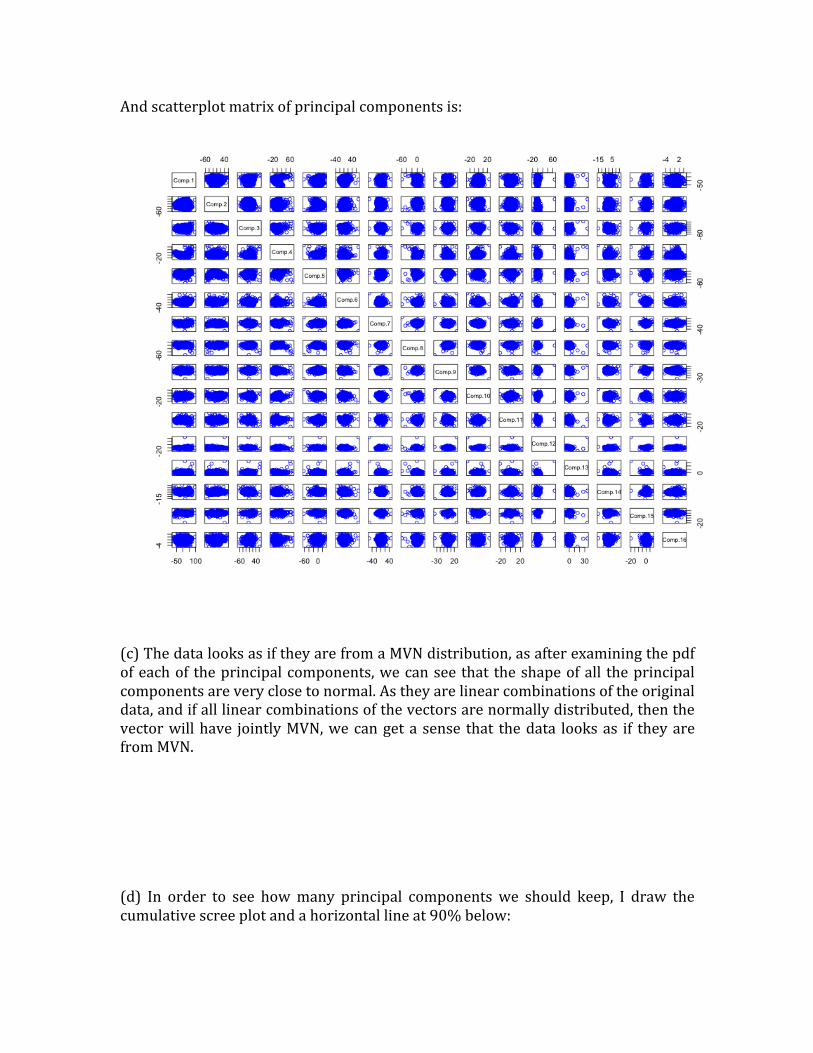
And  scatterplot  matrix  of  principal  components  is:  

     (c)  The  data  looks  as  if  they  are  from  a  MVN  distribution,  as  after  examining  the  pdf  of  each  of   the  principal  components,  we  can  see   that   the  shape  of  all   the  principal  components  are  very  close  to  normal.  As  they  are  linear  combinations  of  the  original  data,  and  if  all  linear  combinations  of  the  vectors  are  normally  distributed,  then  the  vector  will  have   jointly  MVN,  we  can  get  a   sense   that   the  data   looks  as   if   they  are  from  MVN.                (d)   In   order   to   see   how  many   principal   components   we   should   keep,   I   draw   the  cumulative  scree  plot  and  a  horizontal  line  at  90%  below:    

                                       

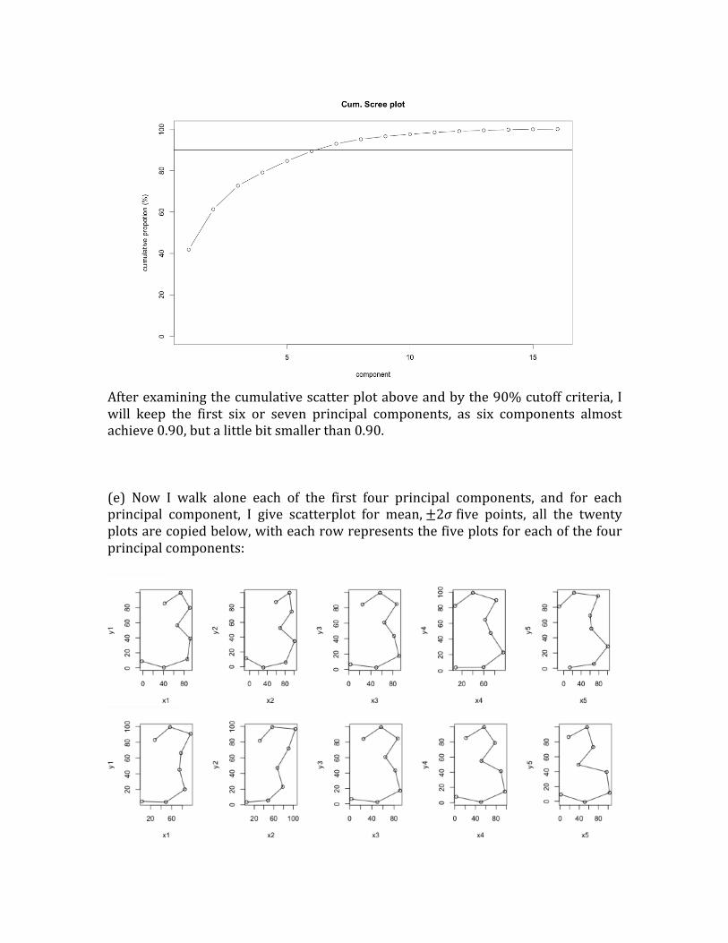
After  examining  the  cumulative  scatter  plot  above  and  by  the  90%  cutoff  criteria,  I  will   keep   the   first   six   or   seven   principal   components,   as   six   components   almost  achieve  0.90,  but  a  little  bit  smaller  than  0.90.        (e)   Now   I   walk   alone   each   of   the   first   four   principal   components,   and   for   each  principal   component,   I   give   scatterplot   for   mean,  ±2𝜎  five   points,   all   the   twenty  plots  are  copied  below,  with  each  row  represents  the  five  plots  for  each  of  the  four  principal  components:    

 

 

 

             (f)  After  combining  the  two  data  sets  together,  I  do  a  PCA  for  the  new  data  set  and  copy  the  scatterplot  matrix  of  principal  components  below.    

                                                   

The   scatterplot  matrix   above   is   too   small,   so   in   order   to   see   if  we   can   see   a   nice  separation  of  observations  corresponding  to  the  digit  3  and  digit  8,  I  draw  another  scatterplot   matrix   which   contains   the   first   several   principal   component.   Now  we  need   to   check   how  many   principal   components   to   keep,   so   I   draw   the   following  scree  plot  and  cumulative  scree  plot:                                      By  the  90%  cutoff  criteria,  I  will  keep  the  first  five  principal  components  and  draw  the  scatterplot  matrix  of  the  first  five  principal  components  as  follows:        

After  examining  the  graphs  above,  we  can  clearly  see  that  there  is  a  relatively  nice  separation  for  the  digit  3  which  are  blue  dots  and  the  digit  8  which  are  red  crossings  in  the  scatterplots  for  principal  component  1  with  principal  component  2,  principal  component   1   with   principal   component   3,   principal   component   1   with   principal  component   4   and   principal   component   1   with   principal   component   5.   So  we   can  separate  digit  3  and  digit  8.            R  code:  #part  a#  x<-­‐c(pendigit3[1,1],pendigit3[1,3],pendigit3[1,5],pendigit3[1,7],pendigit3[1,9],pendigit3[1,11],pendigit3[1,13],pendigit3[1,15])  y<-­‐c(pendigit3[1,2],pendigit3[1,4],pendigit3[1,6],pendigit3[1,8],pendigit3[1,10],pendigit3[1,12],pendigit3[1,14],pendigit3[1,16])  plot(x,y)  lines(x,y)    #part  b  and  d#  x<-­‐pendigit3[  ,c(1,2,3,4,5,6,7,8,9,10,11,12,13,14,15,16)]  spr  <-­‐princomp(x)  U<-­‐spr$loadings  L<-­‐(spr$sdev)^2  Z  <-­‐spr$scores  pairs(Z,pch=c(rep(1,1055)),col=c(rep("blue",1055)))  par(mfrow=c(1,2))  plot(L,type="b",xlab="component",ylab="lambda",main="Scree  plot")  plot(cumsum(L)/sum(L)*100,ylim=c(0,100),type="b",xlab="component",ylab="cumulative  propotion  (%)",main="Cum.  Scree  plot")    plot(cumsum(L)/sum(L)*100,ylim=c(0,100),type="b",xlab="component",ylab="cumulative  propotion  (%)",main="Cum.  Scree  plot")  abline(h=90)      #part  e#  x<-­‐pendigit3[  ,c(1,2,3,4,5,6,7,8,9,10,11,12,13,14,15,16)]  spr  <-­‐princomp(x)  U<-­‐spr$loadings  L<-­‐(spr$sdev)^2  Z  <-­‐spr$scores  par(mfrow=c(1,5))  

v1<-­‐c(mean(x[,1]),mean(x[,2]),mean(x[,3]),mean(x[,4]),mean(x[,5]),mean(x[,6]),mean(x[,7]),mean(x[,8]),mean(x[,9]),mean(x[,10]),mean(x[,11]),mean(x[,12]),mean(x[,13]),mean(x[,14]),mean(x[,15]),mean(x[,16]))  a1<-­‐v1+(-­‐1)*sqrt(L[1])*U[,1]  a2<-­‐v1+(-­‐2)*sqrt(L[1])*U[,1]  a3<-­‐v1  a4<-­‐v1+sqrt(L[1])*U[,1]  a5<-­‐v1+2*sqrt(L[1])*U[,1]  x1<-­‐c(a1[1],a1[3],a1[5],a1[7],a1[9],a1[11],a1[13],a1[15])  y1<-­‐c(a1[2],a1[4],a1[6],a1[8],a1[10],a1[12],a1[14],a1[16])  plot(x1,y1)  lines(x1,y1)    x2<-­‐c(a2[1],a2[3],a2[5],a2[7],a2[9],a2[11],a2[13],a2[15])  y2<-­‐c(a2[2],a2[4],a2[6],a2[8],a2[10],a2[12],a2[14],a2[16])  plot(x2,y2)  lines(x2,y2)    x3<-­‐c(a3[1],a3[3],a3[5],a3[7],a3[9],a3[11],a3[13],a3[15])  y3<-­‐c(a3[2],a3[4],a3[6],a3[8],a3[10],a3[12],a3[14],a3[16])  plot(x3,y3)  lines(x3,y3)    x4<-­‐c(a4[1],a4[3],a4[5],a4[7],a4[9],a4[11],a4[13],a4[15])  y4<-­‐c(a4[2],a4[4],a4[6],a4[8],a4[10],a4[12],a4[14],a4[16])  plot(x4,y4)  lines(x4,y4)    x5<-­‐c(a5[1],a5[3],a5[5],a5[7],a5[9],a5[11],a5[13],a5[15])  y5<-­‐c(a5[2],a5[4],a5[6],a5[8],a5[10],a5[12],a5[14],a5[16])  plot(x5,y5)  lines(x5,y5)      #part  f#  total  <-­‐  rbind(pendigit3,  pendigit8)  Y<-­‐total[  ,c(1,2,3,4,5,6,7,8,9,10,11,12,13,14,15,16)]  spr2<-­‐princomp(Y)  U2<-­‐spr2$loadings  L2<-­‐(spr2$sdev)^2  Z2  <-­‐spr2$scores  pairs(Z2,pch=c(rep(1,1055),rep(3,1055)),col=c(rep("blue",1055),rep("red",1055)))    par(mfrow=c(1,2))  plot(L2,type="b",xlab="component",ylab="lambda",main="Scree  plot")  

plot(cumsum(L2)/sum(L2)*100,ylim=c(0,100),type="b",xlab="component",ylab="cumulative  propotion  (%)",main="Cum.  Scree  plot")  pairs(Z2[  ,c(1,2,3,4,5)],pch=c(rep(1,1055),rep(3,1055)),col=c(rep("blue",1055),rep("red",1055)))    pairs(Z2[  ,c(1,2,3,4,5)],pch=c(rep(1,1055),rep(3,1055)),col=c(rep("blue",1055),rep("red",1055)))  abline(h=90)                                        3.  Solution:  Use  10-­‐fold  cross  validation  to  report  misclassification  rates  of  the  four  classifiers  as  follows:    (1)  LDA  The  10-­‐fold  cross  validation  misclassification  rate  is  0.0014.    (2)  Nearest  Centroid  rule  The  10-­‐fold  cross  validation  misclassification  rate  is  0.03507109.    (3)  QDA  The  10-­‐fold  cross  validation  misclassification  rate  is  0.0024.    (4)  5-­‐Nearest  Neighbors  The  10-­‐fold  cross  validation  misclassification  rate  is  0.    We  can  use  the  following  bar  plot  to  report  the  results  above:  

   

             4.  Solution:    

   

 5.  Solution:  The  code  below  is  a  pseudo-­‐code  in  R  for  10-­‐fold  cross  validation  calculation  in  the  two  questions  above.    cross_validation <- function(X,y,V=10,classify_fun,predict_fun){ n = length(y) fold_size = ceiling(n/V) index = sample(n,n) CVerror = 0 for (v in 1:V){ temp = ((v-1)*fold_size):(min(v*fold_size,n)) test_index = index[temp] train_index = index[-temp] traindata = X[train_index,] trainy = y[train_index] testdata = X[test_index,] testy = y[test_index] model = classify_fun(traindata,trainy) prediction = predict_fun(model,testdata) CVerror = CVerror + sum(prediction!=testy) } CVerror = CVerror/n return(CVerror) }