a

CSIS Discussion Paper (University of Tokyo), No.86

Nonlinearity of Housing Price Structure:

Assessment of Three Approaches to Nonlinearity in the Previously Owned Condominium Market in the Tokyo Metropolitan Area

Chihiro SHIMIZU*

Kiyohiko G. NISHIMURA† Koji KARATO‡

First Draft: May 28,2007 This Version: May 1, 2010

Abstract

This paper examines three methods that explicitly take nonlinearity into account in hedonic price estimation: (1) a switching regression model (SWR) in parametric estimation, (2) a continuous dummy variable model (DmM) in non-parametric estimation, and (3) a generalized additive model (GAM) in semi-parametric estimation. These non-linear estimation methods are applied to the previously owned condominium market in the 23 wards of Tokyo, alongside a linear parametric model as a reference. We find that these nonlinear estimation methods not only increase explanatory power but also yield very similar estimates with respect to the shape of nonlinearity. However, the out-of-sample predictive power of these non-linear estimation methods is inferior to that of a reference linear parametric estimation method, suggesting that these methods are sensitive to sampling biases. Keywords: hedonic model, nonlinearity, structure change, switching regression model, generalized additive models.

JEL Classification: C31 - Cross-Sectional Models; Spatial, R31 - Housing Supply and Markets.

* Associate Professor, Department of International Economics and Business Administration, Reitaku University 2-1-1 Hikarigaoka, Kashiwa-Shi, Chiba, 277-8686 Japan Tel. +81-(0)4-7173-3439, Fax. +81-(0)4-7173-1100 e-mail: cshimizu@reitaku-u.ac.jp † Deputy Governor of the Bank of Japan. Most contribution was made in the development stage of this research, before he joined its Policy Board. ‡ Associate Professor, Faculty of Economics, University of Toyama

1

Nonlinearity of Housing Price Structure:

Assessment of Three Approaches to Nonlinearity in the Previously Owned Condominium Market in the Tokyo Metropolitan Area

1. Introduction

Researches on hedonic housing price models typically assume a linear structure – either linear

with respect to explanatory variables or in some transformation (typically, a logarithm) of them.

In other cases, both response and explanatory variables are transformed but their relationship is

assumed to be linear (Cropper, Deck and McConnel (1988), Halvorson and Pollakowski (1981),

Rasmussen and Zuehlke (1990)). The premise behind this practice is that a linear structure,

possibly coupled with some functional transformation of variables, is sufficiently flexible to

account for the complexity of housing price formation.

In housing markets, however, there are some signs that the assumption of a linear structure

(with fixed transformation of variables) may not capture the complexity. For example, markets

may be segmented into several submarkets with very different coefficients for explanatory

variables that cannot be captured through a linear structure with functional transformation of the

variables (Bourassa, Hoesli and Peng (2003), Goodman(2003)). One possible example may be

the previously owned condominium market in Tokyo, which consists of “studio”, “family-unit”,

and “luxury” submarkets, each with different buyer-seller characteristics (Shimizu, Nishimura

and Asami (2004)). Another example may be the effect of building age, which is often argued to

have a rather complicated relationship with price in the Tokyo market because of somewhat

unpredictable renovation activities. This complexity may not be captured well by pre-specified

functional transformation of the variable.

2

In the literature, several attempts have been made to cope with this “genuine” nonlinearity,

that is, nonlinearity that cannot be captured through pre-specified functional transformation (Bin

(2004), Clapp (2003), Meese and Wallace (1991), Pace (1993), Pace (1998), Thorsnes and

McMillen (1998), Ramazan and Yang (1996)). In this paper, we examine three among these

attempts: a switching regression model in parametric estimation, a continuous dummy variable

model in non-parametric estimation, and a generalized additive model in semi-parametric

estimation.

Firstly, the switching regression model (SWR) is an extension of linear models, but assumes

that a market is segmented into several submarkets with different coefficients for explanatory

variables (Goodman and Thibodeau (2003), McMillen (1994)). Coefficients are assumed to be

different across segments but the same within each segment. The segmentation structure is

estimated through segment dummy variables. Motivated by the apparent market segmentation of

the abovementioned Tokyo condominium market, Shimizu and Nishimura (2007) applied this

approach to the hedonic price model of this market.

Secondly, the continuous dummy variable model (DmM) overcomes restrictions on

functional form imposed by linear models, or in general, models with pre-specified functional

forms. For an explanatory variable to be assumed to have nonlinear effects, “continuous dummy

variables” are constructed continuously with a certain bandwidth and estimated by OLS.

Although this OLS estimation is parametric, the model can be considered as a non-parametric

method since the explanatory variable in question is modeled and estimated as a linear

combination of these continuous dummy variables.1

1 There is no clear definition concerning the differences between parametric regression and non-parametric regression (Yatchew, (2003))．

3

Thirdly, a generalized additive model (GAM) is employed to make the continuous dummy

variable model’s bandwidth flexible and determined in the most fitted way to explain the data.

Here, flexible bandwidth means spline fitting. There are several methods of doing this. For

example, Hastie and Tibshirani (1990) use the backfitting algorithm. In this paper, we have used

a more generalized version, Modified Generalized Cross Validation (MGCV) algorithm by Wood

(2004).

The purpose of this paper is two-folded. Firstly, we examine how important non-linearity is

in hedonic price models. In particular, we investigate how much these non-linear estimation

methods improve the explanatory power of the price model compared with a reference linear

model, and how consistent the results of these methods are with one another concerning the shape

of the non-linearity. Secondly, we explore the predictive power of these non-linear estimation

methods. We conduct an out-of-sample accuracy comparison of these models with the reference

linear model.

In section 2, the data used in this study are explained and the estimation models; the SWR,

DmM, and GAM models, which take into account the nonlinearity, are set up, and in section 3,

assessment of Non-linearity. In section 4, we compare the predictive power of the non-linear

estimation methods. Section5 provides a conclusion.

4

2.Data and Three Nonlinear Estimation Methods of a Hedonic Price Equation

2.1. Data and a Reference Linear Estimation

2.1.1. Tokyo Condominium Markets and Possible Sources of Complex Nonlinearity

We examine the previously owned condominium market of the Tokyo metropolitan area, or

specifically, all of its 23 wards. This area spans 621.97 square kilometers with a population of

8,489,653 in 2005. Tokyo has a long history of more than 500 years as a political and business

center of Japan and has evolved gradually to its current state of complexity and heterogeneity.

In particular, Tokyo condominium markets have evolved alongside the vast expansion of the

suburban railway and subway systems. These condominiums have been designed and targeted for

people working in Tokyo central business districts (CBD) and/or enjoying amenities found in

central areas. Thus, many researches about Tokyo condominium price structure have found that

not only the physical characteristics of a condominium unit such as (1) floor space and (2)

building age, but also (3) time to the nearest train station and (4) time to the nearest terminal

station (a proxy for vicinity to the CBD) are the most important determinants of condominium

prices. In fact, many studies found that these four variables account for almost 70% of the

variation in Tokyo condominium prices (Ohnishi et al (2010)). Taking account of these facts, we

have chosen these four explanatory variables as key variables in the following analysis.

There are several possible sources suggesting a complex nonlinear relationship between key

variables and the condominium price. Firstly, it has often been pointed out that Tokyo

condominium markets are segmented into three distinctive sub-markets (Shimizu, Nishimura and

Asami (2004)). Relatively small condominium units are often purchased for investment purposes

by property investors or for residential purposes by single households, while slightly larger ones

are bought by small households such as the so-called double-income no-kid (DINK) households.

5

In contrast, family households mostly purchase condominium units larger than a certain size. In

addition, there are segments of luxury units. Although exact segmentation of the market is hard to

determine, it is likely that these different segments have noticeably different pricing structures,

leading to complex nonlinear price effects on key variables, particularly on floor space.2

Secondly, the effects of “building age” (number of years since construction) might be very

complex in nature, reflecting the heterogeneity of condominium owners. It is natural to expect

that previously owned condominium unit prices decrease as time after construction increases

because of the physical deterioration. 3 Moreover, we also have to consider recent marked

advances in technology in construction and facilities. They have a complicated effect on the

“economic deterioration” of exiting condominium units. Also, renovation of old facilities, both in

a particular unit and in the building to which it belongs greatly changes the value of the

condominium unit. Renovation may involve not only individual but also collective decisions of

condominium owners, which leads to added complexity.4

Thirdly, with respect to the variable “time to the nearest station”, there are two conflicting

effects of the vicinity to the station. Areas near a railway station have more shops and more

convenient transport links, whereas they often suffer from a lack of parks and a poor natural

environment. Moreover, the value attached to these environmental factors may differ

substantially between various segments of households.5 This suggests a complex nonlinearity that

2 In a related topic, Asami and Ohtaki, 2000 and Thorsnes and McMillen, 1998 pointed out that there is nonlinearity between land area and land value. 3 The lifespan of houses is remarkably short in Japan; the average lifespan is 30 years. (White paper by the Ministry of Land, Infrastructure, Transport and Tourism, 2009) 4 Bid prices are likely to differ between consumers who prefer new facilities and those who do not. They may be also affected by an income constraint, i.e., between high-income and low-income households. Because a depreciation curve with respect to the number of years since construction is a particularly important indicator of collateral assessment for housing loans, an earlier study focusing on this variable was reported (Clapp and Giaccotto, 1998). 5 In Japan, households, including single and DINK households, expressing a preference for convenience will probably buy property in areas near a station, while family households, particularly those with children, will tend to select areas further from the nearest station.

6

cannot be captured by a simple functional transformation of variables. A similar argument applies

to the “travel time to the CBD” variable.

2.1.2. Brief Description of Data

This study utilizes information published in the “Shukan Jutaku Joho” (Weekly Housing

Information Magazine) by Recruit Co., Ltd., one of the largest vendors of residential market

information in Japan. The Recruit dataset covers the 23 special wards of Tokyo for the period

2003 to 2006. It contains 40,353 listings. This database is the most comprehensive one available

to date on the previously owned condominium market in Tokyo, containing location, property

characteristics, and a good proxy of transaction prices, as explained below. It should be noted that

information on actual transaction prices is not available in Japan.

Shukan Jutaku Joho provides time-series of housing prices from the week they are first

posted until the week they are removed due to successful transaction.6 We use only the price in

the final week. This final-week price is shown in our follow-up study to be a good proxy of the

actual contract price in the transaction.7

Transportation convenience at each point was first represented by “time to the nearest

station” (TS) 8 and “travel time to the CBD” (TT). 9

As information regarding the characteristics of previously-owned condominiums themselves,

information on “Floor space” (FS), “Age of building” (Age), “Balcony space” (BS), and

6 There are two reasons for the listing of a unit being removed from the magazine: a successful deal or a withdrawal (i.e. the seller gives up looking for a buyer and thus withdraws the listing). We were allowed access information regarding which of the two reasons applied for individual cases and discarded those where the seller withdrew the listing. 7 Recruit Co., Ltd. provided us with information on contract prices for about 24 percent of all listings. Using this information, we were able to confirm that prices in the final week were almost always identical with the contract prices (i.e., they differed at a probability of less than 0.1 percent). 8 Only data related to condominiums within walking distance were extracted, and the walking time to the nearest station (in minutes) was adopted. 9 Travel time to the CBD is measured as follows. The metropolitan area of Tokyo is composed of 23 wards centering on the Tokyo Station area and containing a dense railway network. Within this area, we choose seven railway/subway stations as the central stations, which include Tokyo, Shinagawa, Shibuya, Shinjuku, Ikebukuro, Ueno, and Otemachi. Then, we define travel time to the CBD by the minutes needed to commute to the nearest of the seven stations in the daytime.

7

“Number of units” (NU) was used. In addition, regarding items considered to affect

condominium value, including whether condominiums are on the highest floor, whether they are

on the ground floor, and the direction in which windows face,10 data for analysis were obtained

using relevant data published in the housing magazine, and dummy variables were produced from

the information.

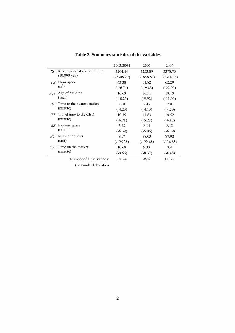
Table 1 shows the list of explanatory variables and their descriptions and Table 2 presents

their summary statistics.

Comparing condominium “resale prices” (RP) first of all, we can see that there was a gradual

upward trend in the average value from 2003 through 2006, with the standard deviation being

larger in 2003-2004 and 2006 than in 2005. There were no significant differences in floor space

(FS), time to the nearest station (TS), balcony space (BS), and total number of units (NU) over the

three points in time. However, with regard to travel time to the CBD (TT), we can see that in

2005 only, the transacted properties were relatively far from the center.

2.1.3. A Reference Linear Estimation Model

Let’s define the models using hedonic equations. The simplest model is set up below as the base

model.

0 1 2 3 4 5 6log / log log logh h i i j j k k l l m mh i j k l m

RP FS a a X a Z a BC a LD a RD a TD ε= + + + + + + +∑ ∑ ∑ ∑ ∑ ∑・ ・ ・

(1)

10 Assuming that the prices of condominiums with windows facing south are higher in Japan, a “south-facing dummy” was set.

8

RP: Resale price of condominium (yen)

Xh: Key variables

FS: Floor space (square meters)

Age: Age of building (months)

TS: Time to the nearest station (minutes)

TT: Travel time to the CBD (minutes)

Zi: Other variables

BS: Balcony space (square meters)

NU: Number of units (units)

TM: Time on the market (weeks)

BC: Building characteristics dummy (first floor dummy, highest floor dummy, south-

facing dummy, and ferroconcrete dummy)

LDj: Location (ward) dummy (j = 0 … J)

RDk: Railway line dummy (k = 0 … K)

TDl: Time dummy (l = 0 … L)

This model for explaining previously owned condominium prices incorporates the floor space

(FS), the number of years since construction (Age), the time to the nearest station (TS), and the

travel time to the CBD (TT), which are variables considered to have important effects on

previously owned condominium prices. In addition to these variables, information such as the

amount of balcony space (BS) and the number of units (NU), available from magazines

containing information on properties, was also incorporated in the models. Such information also

relates to the condominium location or the building characteristics. The railway line dummy

(RDk) takes regional characteristics into account, and the time dummy (TDl) takes temporal

changes in the market into account.

9

The objective of this study is to clarify the price structure of previously owned condominiums

in the 23 wards of Tokyo, with the analysis focusing on the four main variables, FS, Age, TS, and

TT.

2.2. A Switching Regression Model in Parametric Estimation

Next, we modified the base model considering structural change. It is assumed that there are two

points of structural change and three price-bidding curves. For example, if attention is paid to the

location-centered attribute, the following three types of purchases are expected: i) studio type

condominiums in which a single person lives, ii) family type condominiums in which a small

household (for instance, a couple) lives, and iii) luxury type condominiums in which a family

with children lives. Depending on such differences in the entities, the single person and the small

household will probably select a more convenient region, while the family will tend to attach

more importance to the living environment. Hence, TS is also considered to be divided into the

following: i) an area in which households attaching more importance to convenience are located,

ii) an area that is within walking distance of the station but in which a good living environment is

maintained, and iii) an area that requires the use of buses or a car to reach the nearest station.

Given the above perspective, it may be thought that on the whole, three groups having three

different preferences exist in Japan.

As described above, if the market structure is divided into three markets, two points of

structural change should exist for the variable group thought to have nonlinearity. It is unknown,

however, at what point the market structure changes (Jushan and Perron, 1998). Under such

circumstances, the basic model is modified, and an estimate is made through exploratory analysis

of variables thought to have nonlinearity, i.e., FS, Age, TS, and TT. Specifically, the following

10

two dummy variables are introduced on the assumption that the market is divided at points l and

m for each main variable Xh.

( )mhXhlhDm <≤ : if lh ≤ Xh < mh , then 1, otherwise 0

( )XhmhDm ≤ : if mh ≤ Xh , then 1, otherwise 0

ml <

A model such as the one shown below is estimated by introducing the above dummy

variables.

( ) ( ) ( ) ( )( )

( ) ( )( )

0 1 2 3 4 5 6

7 8 9

10

log / log log log

log

log

h h i i j j k k l l m mh i j k l m

hlh Xh mh mh Xh lh Xh mh

h mh Xh

RP FS a a X a Z a BC a LD a RD a TD

a Dm a Dm a X Dm

a X Dm ε

≤ < ≤ ≤ <

≤

= + + + + + + +∑ ∑ ∑ ∑ ∑ ∑

+ + +

+ +

・ ・ ・

(2)

This model is the switching regression model (SWR), and we assume that the regression

model is switched at points l and m. For further information on SWR, see McMillen (1994), and

Shimizu and Nishimura (2007).

2.3. A Continuous Dummy Variable Model in Non-Parametric Estimation

In SWR, we hypothesized that the market structure is divided into three markets and two points

of structural change exist. If there were more than two structural change points, SWR could not

explain the nonlinearity appropriately. We conduct a hedonic model with the four main variables

used as parametric variables in the base model made into dummy variables to estimate the

11

nonlinearity. In forming the dummy variables, an arbitrary bandwidth (β) was set up for each

variable unit. The model obtained by forming the dummy variables based on the four main

variables is referred to as the continuous dummy model (DmM), and can be expressed as:

( ) ( ) ( ) ( )

0 1 2 3 4 5

6 7 8 9

log / log logi i j j k k l l m mi j k l m

RP FS a a Z a BC a LD a RD a TD

a Dm FS a Dm Age a Dm TS a Dm TTρ ρ σ σ ς ς τ τρ σ ς τ

ε

= + + + + + +∑ ∑ ∑ ∑ ∑

+ + + + +∑ ∑ ∑ ∑

・ ・ ・

・ ・ ・ ・

(3)

Dm (Xh): Continuous changing dummy (Dm) variables with a bandwidth (β) determined by main

variables (Xh)

2.4. A Generalized Additive Model in Semi-Parametric Estimation

The DmM model assumes that the previously owned condominium price structure changes

continuously by the bandwidth (β) unit set for each variable. In the actual market, however, it is

not likely that the same bandwidth for all regions of the variable.

In this paper, we have applied calculations based on a more generalized version of DmM, the

generalized additive model (Hastie and Tibshirani(1986),(1990)), hereafter referred to as GAM.

In general, GAM has a structure with the smooth function as follows:

( ) ( )∑∑ +γ=μ h hhm mm XsWg , (4)

where hs are smooth functions of the covariates hX . The model allows for rather flexible

specification of the dependence of response on the covariates. Smooth functions are represented

12

using penalized splines with smoothing parameters selected by generalized cross-validation

(GCV).11

The spline curve calculated based on the Sh functions is a smooth curve passing through the

multiple provided points. Increasing the number of these multiple points increases the fit.

However, a problem similar to the arbitrariness problem in determining bandwidth for DmM

occurs.12

To prevent too much wiggliness in the estimated curve, a special term that penalizes rapid

changes in smooth term is added to the fitting criteria. A common penalty is a smoothing

parameter and an integrated squared second derivative of the function sh.

The estimation model of the hedonic function with GAMs is as follows:

( )0 1 2 3 4 5log / log logh h i i j j k k l l m mh i j k l m

RP FS a s X a Z a BC a LD a RD a TD ε= + + + + + + +∑ ∑ ∑ ∑ ∑ ∑・ ・ ・ (5)

where FSRPlog is the identity link, and ( )hh Xs is an unspecified smooth function for the main

variable (FS, Age, TS, TT). The other terms are predictors ( TDRDLDZ ,,,log ) via a linear

combination term with the parameters 5432 ,,, aaaa .

As well, we employed the Modified Generalized Cross Validation (MGCV) algorithm of

Wood (2006) for calculating the sh functions.13 The MGCV algorithm apply to the equation (5).

11 There are multiple characteristics that can be used as smoothing parameter selection criteria. Generalized cross-validation is one of these criteria (Wood, 2006, pp. 175-177). 12 For example, when performing an approximation based on a cubic curve, the curve’s slope has three distinct sections. In this case, one must determine four knots representing the upper and lower limits of the section. If there are two knots, the splines will be linear; conversely, if there are many knots, the splines will resemble an interpolated line chart showing the data in detail. The form that the splines will take is dependent on the inclination of the slope between the knots, and by increasing their number, it is possible to increase the apparent fit. 13 Hastie and Tibshirani (1990) proposed the backfitting algorithm to fit the smooth function sh. However, the stability of the backfitting algorithm had problems, particularly in datasets with high collinearity among the explanatory variables (Schimek 2009). Another limitation of the GAM estimator is the requirement to select a smoothing parameter (namely, the number of degrees of freedom). A more preferable approach is to determine the degree of smoothing of sh in an endogenous way that depends on the examined data. The automatic selection of the smoothness criteria in the GAM model is possible with the Modified Generalized Cross Validation (MGCV) algorithm of Wood (2004). We applied the MGCV algorithm by using R software (R Development Core Team, 2009) with the MGCV library.

13

3.Assessment of Nonlinearity

3.1. Brief Summary of Estimation Results

Base Model: Linear Model

In this section, we estimate four models, the base model, switching regression model (SWR),

continuous dummy variable model (DmM), and generalized additive model (GAM) using 2005

data.

First, we begin by estimating a base model, as shown in column (i) of Table 3. The

construction cost per square meter is expected to diminish with an increase in condominium size,

but if condominium size and grade are positively correlated, the unit resale price increases with

the size of FS and the other related variables of “Balcony space” (BS) and “Number of units”

(NU). This holds true for BS, because it is expected that BS tends to become larger with

increasing condominium grade. Because of this, BS is considered to be positively estimated for

the condominium scale. NU is a representative index showing the resale price of a condominium

as a whole rather than the price of each unit. For example, because shared space tends to be

ampler as NU increases, this space is considered to affect the condominium unit price.

In addition, convenience in commuting to offices or schools decreases as “time to the nearest

station” (TS) increases. Because there are fewer shops and services and daily life is less

convenient far from stations, condominium resale prices are expected to decrease. Furthermore,

because, in general, more people commute to the CBD, not only commuting expenses but also

commuters’ opportunity costs increase, which is thought to contribute to the decreased

condominium prices.

14

Because there are not only the abovementioned factors that are specific to real estate but also

broad disparities in the housing environment among administrative municipalities or areas along

railway lines, which cannot be considered in the functions estimated in this paper, such

disparities are estimated using the dummy variables.

With the base model as the starting point, it is modified to give the other estimation models

below. In concrete terms, regarding the variables, except for those to be improved as instrumental

variables, all those adopted for the base model are forcibly incorporated into the other models.

Switching Regression Model

In the function that was estimated as the base model, it was assumed that there was a simple

linear relationship between the unit resale price and each variable. However, in actuality, it was

difficult to assume that each variable had a simple linear relationship with the unit resale price.

We conducted a switching regression model (SWR) which is explained in Section 2.2 and

found switching (break) points in four key variables, “Floor space” (FS), “Age of building”

(Age), “Time to the nearest station” (TS), and “Travel time to the CBD” (TT).

In the individual index models (FS, Age, TS, and TT), two structurally different sections were

estimated through an exploratory approach for FS, Age, TS, and TT. By extracting optimum

switching (structural change) points for measurement using AIC as an assessment index, a

structural change test was conducted using the F-test. Two structural change points were detected

for FS, Age, and TS. It was found, however, that there was only one point of structural change for

TT. (Refer to the Appendix.)

The model was formulated on the basis of equation (2) by coupling with the structurally

changed sections extracted using the individual models. The estimation results using the model

15

are shown below. Column (iii) of Table 3 shows estimated coefficients as constant-term dummies

and estimated statistics obtained as cross-terms.

Continuous Dummy Variable Model

An estimation was conducted using a continuous dummy variable model (DmM) in accordance

with the model shown in equation (3). Here, in forming a dummy variable corresponding to each

main variable, the problem was how to set its bandwidth (β). For example, it is unlikely that

consumers change their preference based on 1 m2 of “Floor space” (FS), and because of this, the

bandwidth was set at β = 5. It was considered unproblematic to set β = 1 for the “Age of Building”

(Age), “time to the nearest station” (TS), and “travel time to the CBD” (TT).

( )ρFSDm : 135,,30,25,20,15 K=ρ

( )σAgeDm : 35,,5,4,3,2,1 K=σ

( )ςTSDm : 30,,5,4,3,2,1 K=ς

( )τTTDm : 30,,5,4,3,2,1 K=τ

An Estimation result of DmM is shown in column (ii) of Table 3. The impacts of FS, Age, TS,

and TT change at each specified break point. The result is omitted because there are many

dummy variables (87).

A Generalized Additive Model

Next, an estimation for a generalized additive model (GAM) was conducted. Equation (5) was set

up as a semi-parametric regression model containing both parametric terms and non-parametric

16

terms for smoothing. In column (iv) of Table 3, the determination coefficient adjusted for the

degrees of freedom was 0.814, a value that indicates that the estimated model has an explanatory

power similar to those of DmM and SWR. Note that the explanatory powers of DmM, SWR, and

GAM were improved equivalently compared with that of the base model.

Table 4 shows the estimated performance of the smoothing function by GAM. In column (i),

no great difference was observed in the coefficients other than the smoothed parameters in

comparison with the base model. The degrees of freedom of the smoothing term obtained in

terms of the GCV were not integral. The F-value is a statistic that shows whether there was any

difference between the effect of smoothed cases and that of non-smoothed cases, and it was

indicated that smoothing produced a significant difference between the models.

3.2. Improvement in Explanatory Power

A comparison of the results obtained using the linear model with those obtained using the

continuous dummy model (DmM), switching regression model (SWR), and generalized additive

model (GAM) showed that the predictive power is improved by considering nonlinearity. In

DmM, SWR, and GAM, the determination coefficients adjusted for the degrees of freedom are

0.816, 0.812, and 0.810, an improvement over the 0.775 for the base model. The estimation

parameters related to structural disparities are, in general, accurately estimated.

We examined the predictive power using in-samples with different statistical value. For

comparison of the hedonic models (the base model, DmM, SWR, and GAM) with in-samples, we

use the “Residual Sum of Squares” (RSS) as an evaluation statistic of hedonic models.

The RSS of nonlinear regressions using the SWR (190.708), DmM (185.377), and GAM

(188.708) are smaller than that of the base model (228.471) estimated with the linear model.

17

As a result of comparing the estimated hedonic models with the determination coefficient

adjusted for the degrees of freedom, RSS, DmM, or GAM were found to be the most powerful

hedonic models for estimating the Tokyo metropolitan condominium market.

3.3. Shape of Nonlinearity: Consistency among the Three Methods

A comparison of the estimated shapes of curves for the variables based on the results described

above for a series of estimations revealed the following.

Firstly, we can see the nonlinear relationship between “Floor space” (FS) and unit prices. In

small condominiums with FS of approximately 20 m2, the marginal effect on the unit resale price

per m2 area is high but gradually decreases. It was found, however, that when FS is larger than 80

m2, the marginal effect increases rapidly (see Figures 1 and 2). This tendency is shown by DmM,

SWR, and GAM, but not by the base model. DmM, SWR, and GAM show the same tendency, so

it can be said that this structure is stable. It is seen that in the base model, the relationship

between FS and unit resale prices can be estimated as a monotonically increasing function, and

inaccurate prices can be obtained if the nonlinearity is not taken into account. The theoretical

values for smoothing terms in GAM were normalized so that their total was 0.

This tendency of the relationship is considered to be attributable to differences in the

characteristics and thickness of the market. First, condominiums of approximately 20 m2 for

single-person households are often purchased as investments, whereas purchasers are

increasingly likely to be the persons living in the condominiums as condominium size increases.

Also, regarding construction costs, equipment such as kitchen and restroom equipment (the

construction cost of which is significant) affects the area per unit price. Hence, construction cost

18

per unit tends to increase as the area decreases. For these reasons, it is thought that the unit resale

prices of condominiums with small areas tend to become higher.

The average FS is 61.82 m2. Condominiums of approximately 55 to 70 m2 for families are

supplied in large numbers in Japan, and the market becomes thinner as the condominium area

increases. Because of this, as the area of a condominium increases, a premium is expected to be

placed on units having FS above a certain value.

Next, attention was paid to the relationship between Age and unit resale prices. It was

indicated that in the relationships between price reduction based on the values estimated using the

base model formulated as a simple linear structure and those estimated using the three models,

DmM, SWR, and GAM, greater discrepancies were observed in the price as the age departed

from the average value (16.51 years). Regarding DmM, SWR, and GAM, we found that prices

increased from around 12 years from construction and then decreased after 23 years from

construction (see Figures 3 and 4).

Reasons for the above trend may be that large-scale repairs are first required ten years after

construction. In addition, similar large-scale repairs are required around 20 years after

construction, that is, ten years after the first repairs. Because the rate of depreciation is

particularly rapid from ten to 20 years after construction and because the building price value

subsequently diminishes, the ratio of the land value increases in condominiums (condominium

value is equal to land value and building value), so the depreciation proportion is expected to

decrease.

A comparison of the results obtained using the linear model with those obtained using DmM,

SWR, and GAM showed that the price structure yielded by the linear model differed greatly from

those given by DmM, SWR, and GAM, and that, particularly in the case of the base model, as the

price structure departed from the average price, greater discrepancy was observed.

19

Analysis of the relationship between “time to the nearest station” (TS) and unit resale prices

showed that the price gradient increased slightly when TS was more than 12 minutes, and that it

declined rapidly when TS was more than 17 minutes.

The above tendency was also observed in the cases of DmM, SWR, and GAM (see Figures 5

and 6). Hence, when estimation was conducted using a linear model, price differences increased

when previously owned condominiums were further from the nearest station. First, prospective

buyers selecting a condominium site showed a high preference for transportation convenience,

and when TS was more than ten minutes, the price declined. Because the analysis was made only

for the walking time in this study, it is seen that there is a limiting point when TS is more than ten

minutes. A greater price decline is observed when TS exceeds 17 minutes. This is the limit for the

perceived accessibility to the nearest station on foot, and if TS exceeds this limit, access to the

nearest station is thought to be by an alternative means such as bicycle, bus, or car.

Analysis of the relationship between TT and unit resale prices showed that there was only one

point of structural change (when TT was more than 15 minutes) at which the prices of previously

owned condominiums declined rapidly. A similar tendency was also detected using DmM (β = 1)

and SWR. In other words, previously owned condominium resale price levels did not differ from

one another within an area of about ten minutes from any one of the seven stations set as CBDs,

but upon reaching a travel time of about 15 minutes, the prices declined. When using DmM,

SWR, and GAM, but not the linear model, previously owned condominium resale price levels are

estimated to increase slightly as the travel time increases up to about ten minutes (see Figures 7

and 8). It seems more appropriate to consider this as no price change, rather than as an increased

price, because of the great impact of estimation errors resulting from small changes in price

20

levels. However, previously owned condominium prices declined when TT increased by more

than 15 minutes.

The above analysis indicates that if estimation were to be conducted using the linear model,

previously owned condominium resale price levels would appear to decline more slowly away

from CBDs, and for condominiums farther from CBDs, greater errors would arise. In GAM,

which was affected by the large number of ten-minute samples, it was implicitly estimated that

prices of previously owned condominiums first increased, then declined rapidly, then increased

when TT was ten to 15 minutes, and ultimately declined again. This suggests that the use of GAM

may result in errors if the data used for GAM distribution are discontinuous.

4. Predictive Power of the Nonlinear Estimation Methods

4.1. Out-of-Sample Tests: Accuracy of Predictions

In the in-samples test with RSS, the nonlinear regressions are better than the base model and the

continuous dummy variable model (DmM) and general additive model (GAM) were found to be

the most powerful hedonic models for estimating the Tokyo metropolitan condominium market.

Next, we conducted an examination using out-of-samples data. The Residual Sum of Squares

(RSS) value of DmM was the smallest of the four models. To measure the quality of the fit, we

conducted an out-of-sample prediction analysis. The estimation results in Table 3 are housing

data (number of observations: 9,682) concerning transactions conducted in 2005.

Table 2 presents the summary statistics for the 2003-2004 data (number of observations:

17,913) and 2006 data (number of observations: 11,877) used in the out-of-sample test, along

with the 2005 data.

21

With regard to the out-of-sample test, we verified predictive accuracy by repeatedly and

randomly selecting the same amount of data as the in-sample data used to calculate the four

models (9,682) from the above data and observing the differences between the actual prices and

the forecast prices calculated from the four models.

Specifically, in the linear model estimation, a forecast price ( FSRPlog ) is given by ax ˆˆ nny ′= ,

where nx is the explanatory variables vector in the n th house of data in 2003/ 2004 and 2006

(out-of-sample in multi-period) and a is the estimated coefficients vector (from 2005 data;

shown in Table 2).

In this way, based on the “estimated forecast prices” and “actual prices”, we calculated two

evaluation indexes: the mean absolute percent error (MAPE) and the symmetric mean absolute

percent error (SMAPE) (Bin (2004); Ramazan and Yang (1996)). These were defined as follows:

%100ˆ1

1⋅⎟⎠⎞

⎜⎝⎛ −

= ∑=

N

n n

nnn y

yyN

MAPE ,

( )

%1002ˆ

ˆ11

⋅⎟⎠⎞

⎜⎝⎛

+−

= ∑=

N

n nn

nnn yy

yyN

SMAPE

where ny is actual price of data in 2003-2004 and 2006 (out-of-sample). For each index, if the

forecast price matches the actual price, the value is 0; the greater the discrepancy between the two,

the greater the index value becomes. These calculations were repeated 500 times for each index,

and Table 5 shows their distribution.

First, if we compare the MAPE and SMAPE for 2003 and 2004 with 2006, the values are

relatively high for 2003 and 2004. This difference occurs because we pooled data over a two-year

period covering 2003 and 2004, which meant that temporally distant data were included. As a

result, it is not possible to make a simple comparison between the two periods, so we focused on

the relative difference between the base model (linear model) of the respective tests.

22

In analysis focusing on 2003 and 2004, the linear model had the worst predictive power, and

the more nonlinearity was taken into account, the smaller predictive errors tended to become (in

the following order: SWR, GAM, DmM).

On the other hand, the results for 2006 show that the linear model and DmM had almost the

same predictive accuracy, while predictive accuracy was poor with GAM and particularly SWR.

4.2. Discussion

When we verify predictive accuracy using out-of-sample data, why do the results vary based on

the time period? Why do significant predictive errors occur in 2006 with GAM and SWR in

particular, even though in 2003-2004 the results are the same as for the in-samples test?

We believe it is due to the problems of temporal sample selection bias and structural change,

which we had anticipated.

A problem with the linear model is that is not possible to estimate characteristics toward the

end of the distribution. On the other hand, with calculations that take nonlinearity into account,

while it is possible to properly estimate characteristics at the end of the distribution, once a

change in the data distribution occurs, errors end up being magnified because they are overly

responsive to such characteristics.

This research covers the period from the lengthy recession brought about by the collapse of

the 1980s Bubble to the time when prices started to rise again. Specifically, prices were declining

in 2003-2004, and they hit bottom in 2004. In 2005, prices began to rise, and 2006 saw them

23

increase at a high rate. In other words, there were significant structural changes between 2003-

2004, 2005, and 2006.14

In this kind of situation, it is possible that the distribution of transactions that took place

changed significantly.15

In particular, when there are significant structural changes following macro-level shocks,

nonlinearity conditions change due to changes in the distribution of transactions. As a result,

since the transaction distribution for 2003-2004 was the same as the distribution for 2005, the

same structure was observed for the predictive accuracy of prices with in-sample data as with

out-of-sample data. In 2006, however, when prices began to rise, it is highly probable that

predictive errors were magnified by taking nonlinearity into account.

5. Conclusions

It has been pointed out that, in many countries, the housing market is not homogeneous but rather

is a heterogeneous market. As a result, in recent years it has been noted that nonlinearity should

be taken into account in hedonic model estimates.

All previous studies comparing linear models and nonlinear models have reported that taking

nonlinearity into account increases a model's explanatory power.

However, these previous studies performed in-sample and out-of-sample tests using separate

data from the same point in time. Moreover, in these studies, the calculations for estimating

models that took nonlinearity into account were difficult, and there were also not many data

available: for in-sample data, models were estimated using 1,000 samples or less, while

14 We performed an F-test-based structural change test, which showed structural change at a 1% level of significance for each. 15 Shimizu, Nishimura, and Watanabe (2010) point out that in periods when prices are rising, repeat sales samples (properties that are resold on the market multiple times) tend to increase.

24

predictive accuracy was verified using only a few hundred out-of-sample data items. For our

study, we constructed a unique dataset of around 40,000 items focusing on the area of Tokyo's 23

wards. In addition to estimating models using around 10,000 in-sample data items, we verified

their predictive accuracy using approximately 30,000 out-of-sample items at various points in

time before and after the period for which the model was estimated.

First, with regard to verification of in-sample predictive accuracy, in comparison to a linear

regression model, both the coefficient of determination adjusted for degrees of freedom and the

RSS improved with each of SWR, DmM, and GAM. Furthermore, when we verified the

estimation results by plotting graphs for the four key parameters taking nonlinearity into account,

we obtained almost identical results (i.e., similar slopes) for each of the key parameters of the

three models that accounted for nonlinearity. What’s more, the slopes obtained from the three

models taking nonlinearity into account diverged considerably from the slope of the linear

regression. On this basis, with regard to in-sample data, the findings strongly support the

importance of taking nonlinearity into account.

Next, we verified predictive accuracy using out-of-sample data. In Japan, the hedonic model

is a built-in element of many policies. For example, cost-benefit analysis is obligatory when

implementing urban (re)development projects, and it is the hedonic method that is used to

evaluate their benefit. Financial institutions and the Financial Services Agency use an auto

appraisal system to evaluate mortgage risk, with the hedonic method also being used for the

estimates in this model. In addition, the government is promoting the development of a housing

price index, and here as well the hedonic method is expected to be used as the estimation method.

With regard to the hedonic model used in these economic policies, there is a need for an

accurate, time-oriented model, in order to estimate models using data obtained in the past and use

them in policies employing the estimated parameters.

25

In this research, we estimated a linear model and three models taking nonlinearity into

account using 2005 data, and tested their predictive accuracy with respect to a 2003-2004 data

group and a 2006 data group. The results we obtained show that for 2003-2004, as with the in-

samples test, predictive accuracy was greater for the models taking into account nonlinearity in

comparison to the linear model. However, in 2006, the opposite result was obtained: taking into

account nonlinearity significantly lowered predictive accuracy. It was determined that the reason

for this is that in periods when structural changes occur, taking nonlinearity into account tends to

amplify errors.

To date, no other research on this issue has performed time-oriented out-of-sample tests of

predictive accuracy with such large-scale data. We thus believe this study has provided new

insights into the practical application of hedonic-related research.

26

References

Bin, O. “A Prediction Comparison of Housing Sales Price by Parametric versus Semi-parametric Regressions.”

Journal of Housing Economics 13 (2004), 68–84.

Bourassa, S. C, Hoesli, M., and Peng, V. S. “Do Housing Submarkets Really Matter?” Journal of Housing

Economics 12 (2003), 12–28.

Clapp, J. M. “A Semi Parametric Method for Valuation Residential Locations: Application to Automated

Valuation.” Journal of Real Estate Finance and Economics 27 (2003), 303–320.

Cropper, M., Deck, L., and McConnell, K. “On the Choice of Functional Form for Hedonic Price Functions.”

Review of Economics and Statistics 70 (1988), 668–675.

Gencay, R. and Yang, X. “A Forecast Comparison of Residential Housing Prices by Parametric Versus Semi-

parametric Conditional Mean Estimators.” Economic Letters 52 (1996), 129–135.

Goodman, A. C. and Thibodeau, T. G. “Housing Market Segmentation and Hedonic Prediction Accuracy.”

Journal of Housing Economics 12 (2003), 181–201.

Halvorson, R. and Pollakowski, H. “Choice of Functional Form for Hedonic Price Equations.” Journal of

Urban Economics 10 (1981), 37–49.

Hastie, T. and Tibshirani, R. “Generalized Additive Models (with Discussion).” Statistical Science 1 (1986),

297–318.

Hastie, T. and Tibshirani, R. Generalized Additive Models, Chapman & Hall, 1990.

Jushan, B. and Perron, P. “Estimating and Testing Linear Models with Multiple Structural Changes.”

Econometrica 66 (1998), 47–78.

McCracken, M. W. “Robust out-of-sample inference.” Journal of Econometrics 99 (2000), 195-223.

McMillen, D. P. “Vintage growth and population density: An empirical investigation,” Journal of Urban

Economics 36,(1994), 333–352.

Meese, R. and Wallace, N. “Nonparametric Estimation of Dynamic Hedonic Price Models and the Construction

of Residential Housing Price Indices.” AREUEA Journal, (1991), 308-332.

27

Nelder, J. A. and Wedderburn, R. W. M. Generalized Linear Model. Journal of the Royal Statistical Society,

Series A 135 (1972), 370–384.

Ohnishi, T., Mizuno, T., Shimizu, C. and Watanabe, T., “On the Evolution of the House Price Distribution.”

Center for Price Dynamics (Hitotsubashi University), Discussion Paper, No. 56 (2010).

Pace, R. K. “Nonparametric Methods with Application to Hedonic Models.” Journal of Real Estate Finance

and Economics, Vol. 7 (1993), 185-204.

Pace, R. K. “Appraisal Using Generalized Additive Models.” Journal of Real Estate Research, 15 (1998), 77-

99.

Ramazan, G. and Yang, X. “A Forecast Comparison of Residential Housing Prices by Parametric and

Semiparametric Conditional Mean Estimators.” Economic Letters 52 (1996), 129-135.

Rasmussen, D. and Zuehlke, T. “On the Choice of Functional Form for Hedonic Price Functions.” Applied

Economics 22 (1990), 431–438.

Schimek, M.G. “Semiparametric penalized generalized additive models for environmental research and

epidemiology.” Environmetrics, 20(2009), 699 – 717.

Shimizu, C and Nishimura, K. G. “Pricing Structure in Tokyo Metropolitan Land Markets and its Structural

Changes: Pre-bubble, Bubble, and Post-bubble Periods.” Journal of Real Estate Finance and Economics

36, (2007).

Shimizu, C., Nishimura, K. G. and Asami, Y. “Search and Vacancy Costs in the Tokyo housing market:

Attempt to measure social costs of imperfect information.” Regional and Urban Development Studies,

16, (2004), 210-230.

Shimizu, C., Nishimura, K. G. and Watanabe, T. “House Prices in Tokyo: A Comparison of Repeat-Sales and

Hedonic Measures.” Center for Price Dynamics (Hitotsubashi University) Discussion paper, No. 48

(2010).

Thorsnes, P. and McMillen, D. P. “Land Value and Parcel Size: A Semi Parametric Analysis.” Journal of Real

Estate Finance and Economics 17 (1998), 233–244.

Wood, S. “Stable and efficient multiple smoothing parameter estimation for Generalized Additive Models.”

Journal of the American Statistical Association 99 (2004), 673-686.

28

Wood, S. Generalized Additive Models. An Introduction with R. Chapman and Hall-CRC, Boca Raton, Florida,

(2006).

Wooldridge, J. “Some Alternatives to the Box–Cox Regression Model.” International Economic Review 33

(1992), 935–955.

Yatchew, A. Semi parametric Regression for the Applied Econometrician, Cambridge University Press, (2003).

29

Appendix: Estimation of Switching Regression

A-1. Estimation of Switching (Structural Change) Points by AIC

Assuming that points of price structure change exist in the relationship between unit resale price

and condominium characteristics, structural estimation was carried out using the switched

regression model (SWR). Here, on the assumption that there were two such points in each

relationship, these change points were explored. Under ordinary circumstances, l and m were set

for every main variable Χh. Because it was difficult to optimize them simultaneously,

optimization was carried out for each variable using the base model as a starting point. A model

assessment was performed on the basis of Akaike’s information criterion (AIC).

To confirm whether a structural change occurred in the detected l and m following the above

model estimation, a structural change test was conducted using the F-test.

Estimation Results for “Floor space” (FS)

FS was changed by units of 5 m2 for consistency with DmM. The ranges of combinations of l

and m in ( )mhXhlhDm <≤ and ( )XhmhDm ≤ were l > 15, m < 135, and l < m, and there were 253

combinations. By estimating all the 253 combinations of 253 functions, their AIC values were

compared. Estimation results showed that AIC was minimized at l = 40 and m = 90, and the

determination coefficient adjusted for the degrees of freedom was 0.779, showing an

improvement in the explanatory power. Figure 1 shows the combinations of l and m and changes

in AIC.

30

Estimation Results for “Age of Building” (Age)

On the basis of the distribution of data on Age, the range of analysis was from more than one year

to 35 years. The range of combinations of l and m in ( )mhXhlhDm <≤ and ( )XhmhDm ≤ were l > 2,

m < 35, and l < m, and there were 561 combinations. By estimating all the 561 combinations of

561 functions, their AIC values were compared. Estimation results showed that AIC was

minimized at l = 12 and m = 23, and the determination coefficient adjusted for the degrees of

freedom was 0.801, showing an improvement in the explanatory power compared with that of the

base model. Figure 1 shows the combinations of l and m and changes in AIC.

Estimation Results for “Time to the Nearest Station” (TS)

On the basis of the distribution of data on TS, the range of analysis was from more than one

minute to 30 minutes. The ranges of combinations of l and m in ( )mhXhlhDm <≤ and ( )XhmhDm ≤ were

l > 2, m < 30, and l < m, and there were 300 combinations. By estimating all the 300

combinations of 300 functions, their AIC values were compared. Estimation results showed that

AIC was minimized at l = 12 and m = 17, and the determination coefficient adjusted for the

degrees of freedom was 0.777, showing an improvement in the explanatory power compared with

that of the base model. Figure 1 shows the combinations of l and m and changes in AIC.

Estimation Results for “Travel Time to the CBD” (TT)

On the basis of the distribution of data on TT, the range of analysis was from more than 0 minutes

to 30 minutes. The ranges of combinations of l and m in ( )mhXhlhDm <≤ and ( )XhmhDm ≤ were l ≥ 1,

m < 30, and l < m, and there were 406 combinations. By considering all the 406 combinations of

406 functions, their AIC values were compared. Estimation results showed that AIC was

31

minimized at l = 11 and m = 15, and the determination coefficient adjusted for the degrees of

freedom was 0.777, showing an improvement in the explanatory power compared with that of the

base model. Figure 1 shows combinations of l and m and changes in AIC.

A-2. Confirmation by Structural Change Test

Optimum models were selected from the possible combinations in the above estimation. However,

there was no evidence that structural change occurred in the sections extracted here. To

demonstrate the presence of this change, a structural change test (an F-test) was conducted (Table

3).

Specifically, the three groups divided by l and m in ( )mhXhlhDm <≤ and ( )XhmhDm ≤ were subjected

to an F-test. Group I was set as Х(h<l), group II was set as ( )mhlX <≤ , and group III was set as Х(m<h).

Three tests were conducted, between group I and group II, group II and group III, and group I and

group III, for each variable (FS, Age, TS, and TT). It is particularly important to verify whether or

not there was a structural change between group I and group II, and group II and group III. If a

structural change can be verified, then there is a nonlinear relationship between the unit resale

price and each variable. If the F-test detects structural change between group I and group II and

between group II and group III, but not between group I and group III, then the structure is

different only within l < h < m.

The results of the structural change test showed that a structural change occurred at the two

previously determined values of l and m for FS, Age, and TS with a significant difference of 10%.

For the TT, no structural change was observed between group I and group II, but a structural

change was found to exist between group II and group III. A structural change was also observed

32

between group I and group III. These findings indicated that the structure changed only for m =

15 minutes or more.

1

Table 1. List of analyzed data

Symbols Variables Contents Unit

RP Resale price of condominium

Resale price in last week listed in a housing information magazine 10,000 yen

FS Floor space Floor space m2

Age Age of building:

Number of years since construction

Period between the date when the data is deleted from the magazine and the date of construction of the

building year

TS Time to the nearest station Distance in time (walking time) to the nearest station minute

TT Travel time to the CBD Minimum railway riding time in the daytime to seven terminal stations in 2005*. minute

BS Balcony space Balcony space. m2

NU Number of units Total units of the condominium. unit

TM Time on the market Period between the date when the data appear in the

magazine for the first time and the date when they are deleted.

week

FF First floor dummy The property is on the ground floor 1,

(0,1) on other floors 0.

HF Highest floor dummy The property is on the top floor 1,

(0,1) on the other floors 0.

SD South-facing dummy Window facing south 1，

(0,1) other directions 0.

FD Ferroconcrete dummy Steel reinforced concrete frame structure 1,

(0,1) other structure 0.

LDj (j=0,…,J) Location (Ward) dummy j th administrative district 1,

(0,1) other district 0.

RDk (k=0,…,K) Railway line dummy k th railway line 1,

(0,1) other railway line 0.

TDl (l=0,…,L) Time dummy (quarterly) l th quarter 1,

(0,1) other quarter 0.

*Terminal stations: Tokyo, Shinagawa, Shibuya, Shinjuku, Ikebukuro, Ueno and Otemachi

2

Table 2. Summary statistics of the variables

2003/2004 2005 2006 RP : Resale price of condominium

(10,000 yen) 3264.44 3253.89 3378.73

(-2348.29) (-1858.83) (-2314.76) FS : Floor space

(m2) 63.38 61.82 62.29

(-26.74) (-19.83) (-22.97) Age : Age of building

(year) 16.69 16.51 18.19

(-10.23) (-9.92) (-11.09) TS : Time to the nearest station

(minute) 7.68 7.45 7.8

(-4.29) (-4.19) (-4.29) TT : Travel time to the CBD

(minute) 10.35 14.83 10.52

(-6.71) (-5.23) (-6.82) BS : Balcony space

(m2) 7.88 8.14 8.13

(-6.39) (-5.96) (-6.19) NU : Number of units

(unit) 89.7 88.03 87.92

(-125.38) (-122.48) (-124.85) TM : Time on the market

(minute) 10.68 9.33 8.4

(-9.66) (-8.37) (-8.48) Number of Observations: 18794 9682 11877 ( ): standard deviation

3

Table 3. Estimation results of base model, DmM, SWR, and GAM

(i) Base (ii) SWR (iii) DmM (iv) GAM Coef. t−value Coef. t−value Coef. t−value Coef. t−value

log(FS) 0.047 8.984 −0.094 −4.890 − − log(Age) −0.188 −96.379 −0.086 −24.868 − − log(TS) −0.054 −21.510 −0.046 −16.935 − − log(TT) −0.017 −5.237 −0.009 −2.779 − −

Dm (Xh) − − Yes

DM_FS (40≦FS<90) − −0.387 −5.149 − −

DM_Age (12≦Age<23) − 0.579 11.733 − − DM_TS (12≦TS<17) − 0.216 2.130 − −

DM_FS (90≦FS) − −1.374 −6.058 − − DM_Age (23≦Age) − 0.109 1.521 − −

DM_TS (17≦TS) − 0.773 2.682 − − DM_TT (17≦TT) − 0.458 10.901 − −

log(FS)* DM_FS (40≦FS<90) − 0.110 5.188 − −

log(Age)* DM_Age (12≦Age<23) − −0.241 −14.059 − −

log(TS)* DM_TS (12≦TS<17) − −0.099 −2.522 − −

log(FS)* DM_FS (90≦FS) − 0.339 6.711 − −

log(Age)* DM_Age (23≦Age) − −0.106 −4.831 − −

log(TS)* DM_TS (17≦TS) − −0.296 −2.993 − −

log(TT)* DM_TT (17≦TT) − −0.163 −11.236 − −

s(Xh) − − − Yes

BS 0.012 4.471 0.009 3.637 0.007 2.832 0.008 3.198 NU 0.020 10.190 0.031 16.890 0.031 16.882 0.032 17.477 TM −0.006 −3.331 −0.007 −4.442 −0.007 −4.580 −0.007 −4.536 FF −0.034 −6.198 −0.042 −8.286 −0.043 −8.549 −0.043 −8.412 HF 0.054 5.365 0.052 5.579 0.054 5.803 0.054 5.892 FD −0.012 −3.226 −0.015 −4.496 −0.015 −4.361 −0.016 −4.733 SD 0.003 0.965 0.007 2.280 0.008 2.565 0.008 2.525 LD Yes Yes Yes Yes RD Yes Yes Yes Yes TD Yes Yes Yes Yes

Const. 3.931 155.275 4.242 63.250 3.990 155.802 3.475 299.292

Residual Sum of Squares 228.471 190.708 185.337 188.166 Adj. R2 0.775 0.812 0.816 0.810

Number of Observations. 9,682 9,682 9,682 9,682

4

Table 4. Estimated smoothing parameters

Estimated d.f F-statistics p-value

sFS(FS) 7.573 33.41 0.000

sAge(Age) 8.518 1366.12 0.000

sTS(TS) 7.779 96.77 0.000

sTT(TT) 8.983 26.72 0.000

GCV score: 0.019

Deviance explained: 81.60% Number of Observations: 9,682

(Note: GCV score is an indicator of the error of the generalized cross-validation method, and the ‘deviance explained’ is an index of the applicability of the theoretical figure to the actual performance.)

Table 5. The mean absolute percent error (MAPE) and the symmetric mean absolute

percent error (SMAPE)

MAPE SMPAE t-1: [2003&2004] t+1:[2006] t-1: [2003&2004] t+1:[2006] mean s.d. mean s.d. mean s.d. mean s.d.

Base 25.457 0.081 3.337 0.012 15.295 0.049 3.357 0.011SWR 21.566 0.084 19.155 0.082 12.97 0.05 19.115 0.08DmM 15.519 0.073 3.337 0.012 9.307 0.043 3.355 0.012GAM 19.079 0.079 9.678 0.054 10.945 0.041 9.58 0.053

* The experiment is repeated 500 times per t-1[year2003&2004], t+1[year2006]. t=year2005 * Number of Observations: year2005=9682, year2003&2004=19879 and year2006=11,877.

5

Table A-1. Test results for structural change test (Prob>0)

Ⅰ vs. Ⅱ Ⅱ vs. Ⅲ Ⅰ vs. Ⅲ

X(h<=l) vs. X(l<h<=m) X(l<h<=m) vs. X(m<h) X(h<=l) vs. X(m<h)

FS: Floor space (m2) 0.00003 0.00000 0.00000

Age: Age of building (months) 0.00179 0.08101 0.05582

TS: Time to the nearest station (minutes) 0.00000 0.00001 0.01115

TT: Travel time to the CBD (minutes) 0.22236 0.00000 0.00000

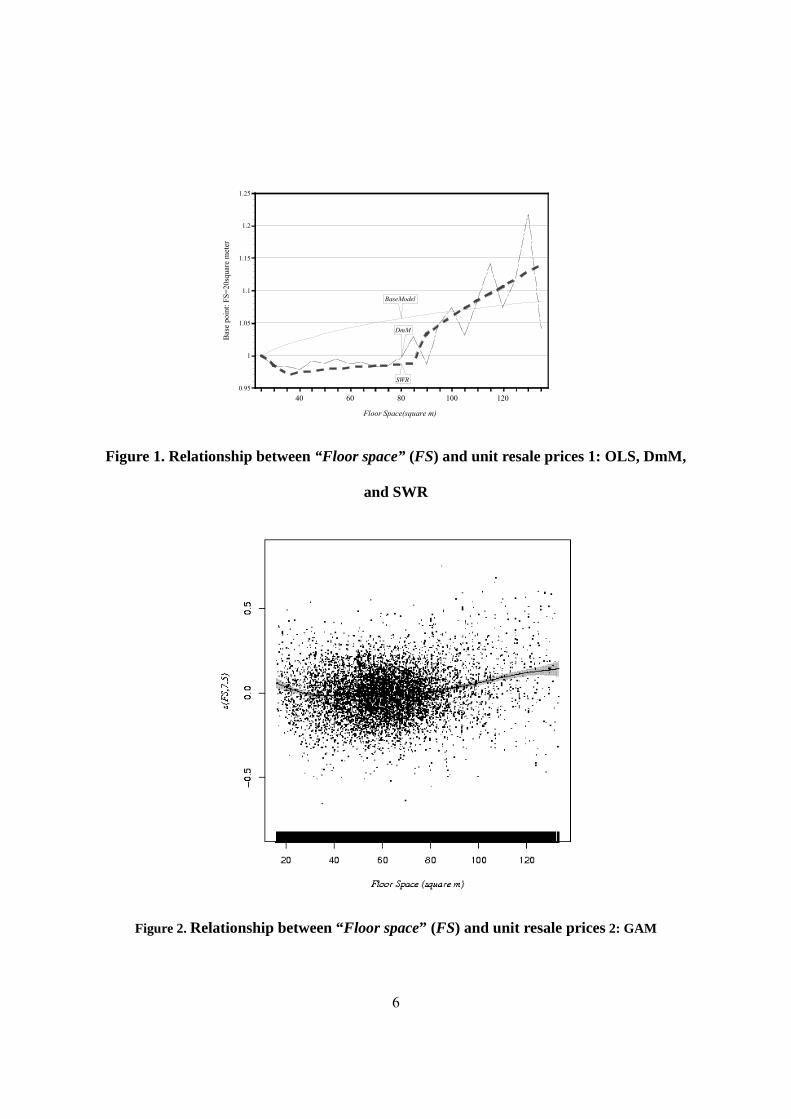
6

Figure 1. Relationship between “Floor space” (FS) and unit resale prices 1: OLS, DmM,

and SWR

Figure 2. Relationship between “Floor space” (FS) and unit resale prices 2: GAM

0.95

1

1.05

1.1

1.15

1.2

1.25

40 60 80 100 120

BaseModel

DmM

SWR

Bas

e po

int:

FS=2

0squ

are

met

er

Floor Space(square m)

7

Figure 3. Relationship between “Age of building” (Age) and unit resale prices 1: OLS,

DmM, and SWR

Figure 4. Relationship between “Age of building” (Age) and unit resale prices 2: GAM

0.5

0.6

0.7

0.8

0.9

1

5 10 15 20 25 30

BaseModel

DmM

SWR

Bas

e po

int:

Age

=1

Age of building(Year)

8

Figure 5. Relationship between “Time to the nearest station” (TS) and unit resale prices 1:

OLS, DmM, and SWR

Figure 6. Relationship between “Time to the nearest station” (TS) and unit resale prices 2:

GAM

0.65

0.7

0.75

0.8

0.85

0.9

0.95

1

5 10 15 20 25

BaseModel

DmM

SWRBas

e po

int:

TS=2

Time to Nearest Station(Munites)

9

Figure 7. Relationship between “Travel time to the CBD” (TT) and unit resale prices 1 OLS,

DmM, and SWR

Figure 8. Relationship between “Travel time to the CBD” (TT) and unit resale prices 2: GAM

0.86

0.88

0.9

0.92

0.94

0.96

0.98

1

1.02

5 10 15 20 25 30

BaseModel

DmM(bandwidth=1)

SWR

DmM(bandwidth=5)

Bas

e po

int:

TT=1

Travel Time to CBD(Minutes)

10

Figure A-1. AIC/three segments in SWR

"Floor space" "Age of building"

"Time to the nearest station" "Travel time to the CBD"

-36234 -36224.6 -36215.2 -36205.8 -36196.4 -36187 -36177.6 -36168.2 -36158.8 -36149.4 above

z=-36175.3-1.933*x-6.554*y+0.221*x*x-0.134*x*y+0.22*y*y

-36234.36 -36224.9 -36215.5 -36206.05 -36196.6 -36187.2 -36177.74 -36168.3 -36158.87 -36149.43 above

z=-36225.1-5.263*x-0.24*y+0.776*x*x-0.445*x*y+0.14*y*y

-36325 -36310.5 -36296 -36281.5 -36267 -36252.5 -36238 -36223.5 -36209 -36194.5 above

z=-36229.45+1.573*x-3.253*y+0.015*x*x-0.024*x*y+0.024*y*y

-37226.07 -37103.46 -36980.85 -36858.25 -36735.64 -36613.03 -36490.4 -36367.8 -36245.2 -36122.6 above

z=-36963.63-35.608*x-20.953*y+4.047*x*x-2.249*x*y+1.079*y*y