open source matlab implementation of consistent
TRANSCRIPT
Open Source MATLAB Implementation of
Consistent Discretisations on Complex Grids
Knut–Andreas Lie Stein Krogstad Ingeborg S. LigaardenJostein R. Natvig Halvor Møll Nilsen Bard Skaflestad
Received: date / Accepted: date
Abstract
Accurate geological modelling of features such as faults, fractures orerosion requires grids that are flexible with respect to geometry. Such gridsgenerally contain polyhedral cells and complex grid cell connectivities.The grid representation for polyhedral grids in turn affects the efficientimplementation of numerical methods for subsurface flow simulations. Itis well known that conventional two-point flux-approximation methodsare only consistent for K orthogonal grids and will therefore not convergein the general case. In recent years, there has been significant researchinto consistent and convergent methods, including mixed, multipoint, andmimetic discretisation methods. Likewise, so-called multiscale methodsbased upon hierarchically coarsened grids have received a lot of attention.
The paper does not propose novel mathematical methods but insteadpresents an open-source Matlab® toolkit that can be used as an efficienttest platform for (new) discretisation and solution methods in reservoirsimulation. The aim of the toolkit is to support reproducible researchand simplify the development, verification and validation, and testingand comparison of new discretisation and solution methods on generalunstructured grids, including in particular corner-point and 2.5D PEBIgrids. The toolkit consists of a set of data structures and routines forcreating, manipulating, and visualising petrophysical data, fluid models,and (unstructured) grids, including support for industry-standard inputformats, as well as routines for computing single and multiphase (incom-pressible) flow. We review key features of the toolkit and discuss a genericmimetic formulation that includes many known discretisation methods,including both the standard two-point method as well as consistent andconvergent multipoint and mimetic methods. Apart from the core routinesand data structures, the toolkit contains add-on modules that implementmore advanced solvers and functionality. Herein, we show examples ofmultiscale methods and adjoint methods for use in optimisation of ratesand placement of wells.
1
1 Introduction
Reliable computer modelling of subsurface flow is much needed to overcomeimportant challenges such as sustainable use and management of the earth’sgroundwater systems, geological storage of CO2 to mitigate the anthropologicalincreases in the carbon content of the atmosphere, and optimal utilisation ofhydrocarbon reservoirs. Indeed, the need for tools that help us understandflow processes in the subsurface is probably greater than ever, and increasing.More than fifty years of prior research in this area has led to some degree ofagreement in terms of how subsurface flow processes can be modelled adequatelywith numerical simulation technology.
To describe the subsurface flow processes mathematically, two types of mod-els are needed. First, one needs a mathematical model that describes how fluidsflow in a porous medium. These models are typically given as a set of partialdifferential equations describing the mass-conservation of fluid phases, accom-panied by a suitable set of constitutive relations. Second, one needs a geologicalmodel that describes the given porous rock formation (the reservoir). The geo-logical model is realised as a grid populated with petrophysical or hydrologicalproperties that are used as input to the flow model, and together they makeup the reservoir simulation model. The geological model must also describe thegeometry of the reservoir rock and in particular model geological horizons andmajor faults. This requires grids that are flexible with respect to geometry (andtopology). Stratigraphic grids have been popular for many years and are thecurrent industry standard. These grids are formed by extruding areal grids de-fined along geological surfaces to form volumetric descriptions. However, morecomplex methods based on unstructured grids are gaining in popularity as ameans to modelling complex fault systems, horizontal and multilateral wells,etc. In either case, grids representing realistic reservoirs generally contain poly-hedral cells and complex grid cell connectivities. The grid representation forpolyhedral grids in turn affects the efficient implementation of numerical meth-ods for subsurface flow simulations.
The industry-standard for discretising flow equations is the two-point flux-approximation method, which for a 2D Cartesian grid corresponds to a standardfive-point scheme for the elliptic Poisson equation. Although widely used, thismethod is convergent only if each grid cell K-orthogonal. For hexahedral grids,this means that each cell is a parallelepiped and ~nijKi~nik = 0 in all grid cellsi (here, K is the permeability tensor in cell i and ~nij and ~nik denote normalvectors into two neighbouring cells). Ensuring K-orthogonality is difficult whenrepresenting particular geological features like sloping faults, horizontal wells,etc. Hence, there has in recent years been significant research into mixed [8],multipoint [5], and mimetic [9] discretisation methods that are all consistent andconvergent on rougher grids. Herein, we will focus on low-order, cell-centredmethods that do not require specific reference elements and thus can be appliedto grids with general polygonal and polyhedral cells.
Another major research challenge is the gap between simulation capabilitiesand the level of detail available in current geological models. Despite an as-
2
tonishing increase in computer power, and intensive research on computationtechniques, commercial reservoir simulators can seldom run simulations directlyon highly resolved geological grid models that may contain from one to a hun-dred million cells. Instead, coarse-grid models with grid-blocks that are typicallyten to a thousand times larger are built using some kind of upscaling of the geo-physical parameters [16, 13]. How one should perform this upscaling is nottrivial. In fact, upscaling has been, and probably still is, one of the most activeresearch areas in the oil industry. Lately, however, so-called multiscale methods[17, 15, 18] have received a lot of attention. In these methods, coarsening andupscaling needed to reduce the number of degrees of freedom to a level thatis sufficient to resolve flow physics and satisfy requirements on computationalcosts is done implicitly by the simulation method.
A major goal of the activities in our research group is to develop efficientsimulation methodologies based on accurate and robust discretisation methods;in particular, we have focused on developing multiscale methods. To this end,we need a toolbox for rapid prototyping of new ideas that enables us to eas-ily test the new implementations on a wide range of models, from small andhighly idealised grid models to large models with industry-standard complexity.When developing new computational methodologies, flexibility and low devel-opment time is more important than high code efficiency, which will typicallyonly be fully achieved after the experimental programming is completed andideas have been thoroughly tested. For a number of years, we have thereforedivided our code development in two parts: For prototyping and testing of newideas, we have used Matlab, whereas solvers aimed at high computational per-formance have been developed in a compiled language (i.e., using FORTRAN,C, or generic programming in C++).
This has resulted in a comprehensive set of routines and data structures forreading, representing, processing, and visualising unstructured grids, with par-ticular emphasis on the corner-point format used within the petroleum industryand hierarchical grids used in multiscale methods. To enable other researchersto benefit from our efforts, these routines have been gathered in the MatlabReservoir Simulation Toolbox (MRST), which is released under the GNU Gen-eral Public License (GPL). The first releases are geared towards single- andtwo-phase flow and contain a set of mimetic and multiscale flow solvers and afew simple transport solvers capable of handling general unstructured, polyhe-dral grids.
The main purpose of this paper is to present MRST and demonstrate itsflexibility and efficiency with respect to different grid formats, and in particularhierarchical grids used in multiscale methods. Secondly, we present a class ofmimetic methods that incorporates several well-known discretisation methodsas special cases on simple grids while at the same time providing consistent dis-cretisation on grids that are not K-orthogonal. Finally, we discuss how genericimplementations of various popular methods for pressure and transport easethe study and development of advanced techniques such as multiscale methods,flow-based gridding, and applications such as optimal control or well placement.
3
2 The MATLAB Reservoir Simulation Toolbox
The toolbox has the following functionality for rapid prototyping of solvers forflow and transport:
Grids: a common data structure and interface for all types of grids (unstruc-tured representation); no grid generator but grid factory routines for recti-linear grids, triangular and tetrahedral grids, 2D Voronoi grids, extrusionof areal grids to 2.5D volumetric grids, etc; tutorial examples and a fewrealistic data sets
Input and output: routines for reading and processing industry-standard in-put files for grids, petrophysical parameters, fluid models, wells, boundaryconditions, simulation setup, etc.
Parameters: a data structure for petrophysical parameters (and a few, verysimplified geostatistical routines); common interface to fluid models (Ver-sion 2011a supports incompressible fluid models, but in-house develop-ment version also has support for compressible black-oil fluids, which willlikely be released in future versions of MRST); routines for setting andmanipulating boundary conditions, sources/sinks, well models, etc
Units: MRST works in strict SI units but supports conversion to/from otherunit systems like field-units, etc. Unless reading from an industry-standardinput format, the user is responsible for explicit conversion and consistencyof units1.
Reservoir state: data structure for pressure, fluxes, saturations, . . .
Postprocessing: visualisation routines for scalar cell and face data, etc
Solvers: the toolbox contains several flow and transport solvers which may bereadily combined using an operator splitting framework. In particular, weprovide an implementation of the multiscale mixed finite-element method[4], working on unstructured, polyhedral grids
Linear algebra: MRST relies on Matlab’s builtin linear solvers but these caneasily be replaced by specialised solvers using standard Matlab conven-tions for doing so.
We will now go into more details about some of the components outlinedabove. All code excerpts and explicit statements of syntax refer to release 2011aof MRST. Complete scripts and the data necessary to run most of the examplesin the paper can be downloaded from the MRST webpage [26]. The interestedreader should also review the tutorials included in the current release.
1All examples considered herein are computed using SI units, but other units may be usedwhen reporting parameters and solutions.
4
1
2
3
4
5
6
7
8
1
2
3
4
5
6
7
8
9
10
11
12
13
14
1
2
3
4
5
6
7
cells.faces = faces.nodes = faces.neighbors =
1 10 1 1 0 2
1 8 1 2 2 3
1 7 2 1 3 5
2 1 2 3 5 0
2 2 3 1 6 2
2 5 3 4 0 6
3 3 4 1 1 3
3 7 4 7 4 1
3 2 5 2 6 4
4 8 5 3 1 8
4 12 6 2 8 5
4 9 6 6 4 7
5 3 7 3 7 8
5 4 7 4 0 7
5 11 8 3
6 9 8 5
6 6 9 3
6 5 9 6
7 13 10 4
7 14 10 5
: : : :
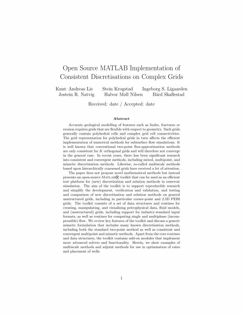
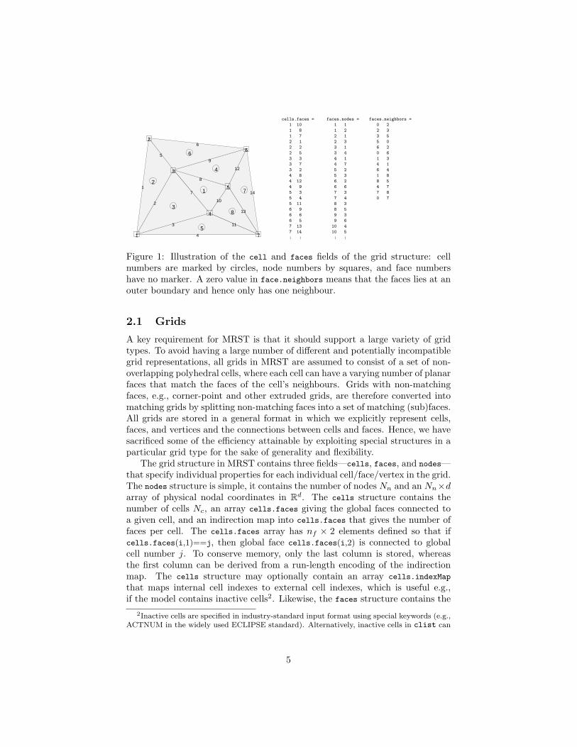
Figure 1: Illustration of the cell and faces fields of the grid structure: cellnumbers are marked by circles, node numbers by squares, and face numbershave no marker. A zero value in face.neighbors means that the faces lies at anouter boundary and hence only has one neighbour.
2.1 Grids
A key requirement for MRST is that it should support a large variety of gridtypes. To avoid having a large number of different and potentially incompatiblegrid representations, all grids in MRST are assumed to consist of a set of non-overlapping polyhedral cells, where each cell can have a varying number of planarfaces that match the faces of the cell’s neighbours. Grids with non-matchingfaces, e.g., corner-point and other extruded grids, are therefore converted intomatching grids by splitting non-matching faces into a set of matching (sub)faces.All grids are stored in a general format in which we explicitly represent cells,faces, and vertices and the connections between cells and faces. Hence, we havesacrificed some of the efficiency attainable by exploiting special structures in aparticular grid type for the sake of generality and flexibility.
The grid structure in MRST contains three fields—cells, faces, and nodes—that specify individual properties for each individual cell/face/vertex in the grid.The nodes structure is simple, it contains the number of nodes Nn and an Nn×darray of physical nodal coordinates in Rd. The cells structure contains thenumber of cells Nc, an array cells.faces giving the global faces connected toa given cell, and an indirection map into cells.faces that gives the number offaces per cell. The cells.faces array has nf × 2 elements defined so that ifcells.faces(i,1)==j, then global face cells.faces(i,2) is connected to globalcell number j. To conserve memory, only the last column is stored, whereasthe first column can be derived from a run-length encoding of the indirectionmap. The cells structure may optionally contain an array cells.indexMap
that maps internal cell indexes to external cell indexes, which is useful e.g.,if the model contains inactive cells2. Likewise, the faces structure contains the
2Inactive cells are specified in industry-standard input format using special keywords (e.g.,ACTNUM in the widely used ECLIPSE standard). Alternatively, inactive cells in clist can
5
dx = 1−0.5*cos((−1:0.1:1)*pi);x = −1.15+0.1*cumsum(dx);G = tensorGrid (x , sqrt (0:0 .05 :1));plotGrid (G );
load seamount % Matlab standard datasetg = pebi( triangleGrid ([ x (:) y (:)]));G = makeLayeredGrid (g , 5);plotGrid (G ), view(−40, 60),
G = processGRDECL ( ...simpleGrdecl ([20, 10, 5], 0.12 ));
plotGrid (G , 'FaceAlpha',0.8);plotFaces (G , find ( G.faces.tag >0), ...
'FaceColor','red' );view (40,40), axis off
grdecl = readGRDECL ( 'SAIGUP.GRDECL');G = processGRDECL ( grdecl );plotGrid (G , 'EdgeAlpha',0.1);view(−80,50), axis tight off
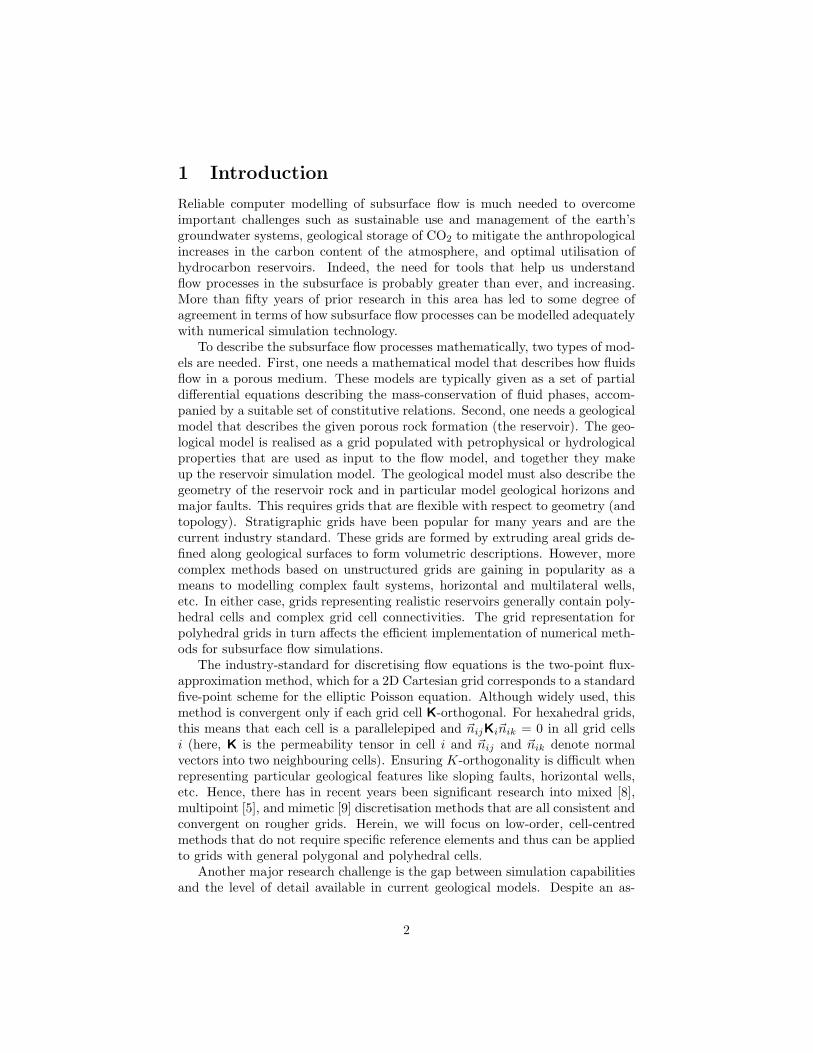
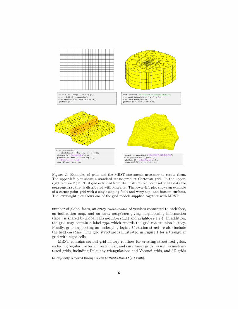
Figure 2: Examples of grids and the MRST statements necessary to create them.The upper-left plot shows a standard tensor-product Cartesian grid. In the upper-right plot we 2.5D PEBI grid extruded from the unstructured point set in the data fileseamount.mat that is distributed with Matlab. The lower-left plot shows an exampleof a corner-point grid with a single sloping fault and wavy top- and bottom surfaces.The lower-right plot shows one of the grid models supplied together with MRST.
number of global faces, an array faces.nodes of vertices connected to each face,an indirection map, and an array neighbors giving neighbouring information(face i is shared by global cells neighbors(i,1) and neighbors(i,2)). In addition,the grid may contain a label type which records the grid construction history.Finally, grids supporting an underlying logical Cartesian structure also includethe field cartDims. The grid structure is illustrated in Figure 1 for a triangulargrid with eight cells.
MRST contains several grid-factory routines for creating structured grids,including regular Cartesian, rectilinear, and curvilinear grids, as well as unstruc-tured grids, including Delaunay triangulations and Voronoi grids, and 3D grids
be explicitly removed through a call to removeCells(G,clist).
6
created by extrusion of 2D shapes. Most important, however, is the supportfor the industry-standard corner-point grids given by the ECLIPSE input deck.In Figure 2 we show four examples of grids and the commands necessary tocreate and display them. The rectilinear grid is generated by the grid-factoryroutine tensorGrid, which takes one vector of grid nodes per spatial dimensionas input and creates the corresponding tensor-product mesh. To generate the2.5D PEBI grid, we start with an unstructured point set (seamount.mat) anduse triangleGrid to generate a Delauny grid, from which a 2D Voronoi grid isgenerated using pebi. Then this areal grid is extruded to a 3D model consistingof five layers using the routine makeLayeredGrid. In the third plot, we have usedthe routine simpleGrdecl to generate an example of an ECLIPSE input streamand then processGRDECL to process the input stream and generate a corner-pointgrid. The lower-right plot shows a realistic reservoir model where we have usedreadGRDECL to read the grid section of an ECLIPSE input deck; the routine readsthe file and creates an input stream on the same format as simpleGrdecl.
As we will see below, specific discretisation schemes may require other prop-erties not supported by our basic grid class: cell volumes, cell centroids, faceareas, face normals, and face centroids. Although these properties can be com-puted from the geometry (and topology) on the fly, it is often useful to pre-compute and include them explicitly in the grid structure G. This is done bycalling the generic routine G=computeGeometry(G).
2.2 Petrophysical Parameters
All flow and transport solvers in MRST assume that the rock parameters are rep-resented as fields in a structure. Our naming convention is that this structure iscalled rock, but this is not a requirement. The fields for porosity and permeabil-ity, however, must be called poro and perm, respectively. Whereas petrophysicalparameters are often supplied for all cells (active and inactive) in a model, therock and grid structures in MRST only represent the active cells. The porosityfield rock.poro is therefore a vector with one value for each active cell in the cor-responding grid model. For models with inactive cells, the field cells.indexMap
in the grid structure contains the indices of the active cells sorted in ascendingorder. If p contains porosity values for all cells, this porosity distribution isassigned to the rock structure by the call rock.poro = p(G.cells.indexMap).
The permeability field rock.perm can either contain a single column for anisotropic permeability, two or three columns for a diagonal permeability (intwo and three spatial dimensions, respectively), or three or six columns fora symmetric, full tensor permeability (in two and three spatial dimensions,respectively). In the latter case, cell number i has the permeability tensor
Ki =[K1(i) K2(i)K2(i) K3(i)
], Ki =
K1(i) K2(i) K3(i)K2(i) K4(i) K5(i)K3(i) K5(i) K6(i)
,where Kj(i) is the entry in column j and row i of rock.perm. Full-tensor, non-symmetric permeabilities are currently not supported in MRST. In addition to
7
0 10 20 30 40 500
5
10
15
20
0.2 0.25 0.3 0.35 0.4
25 50 100 200 400 800
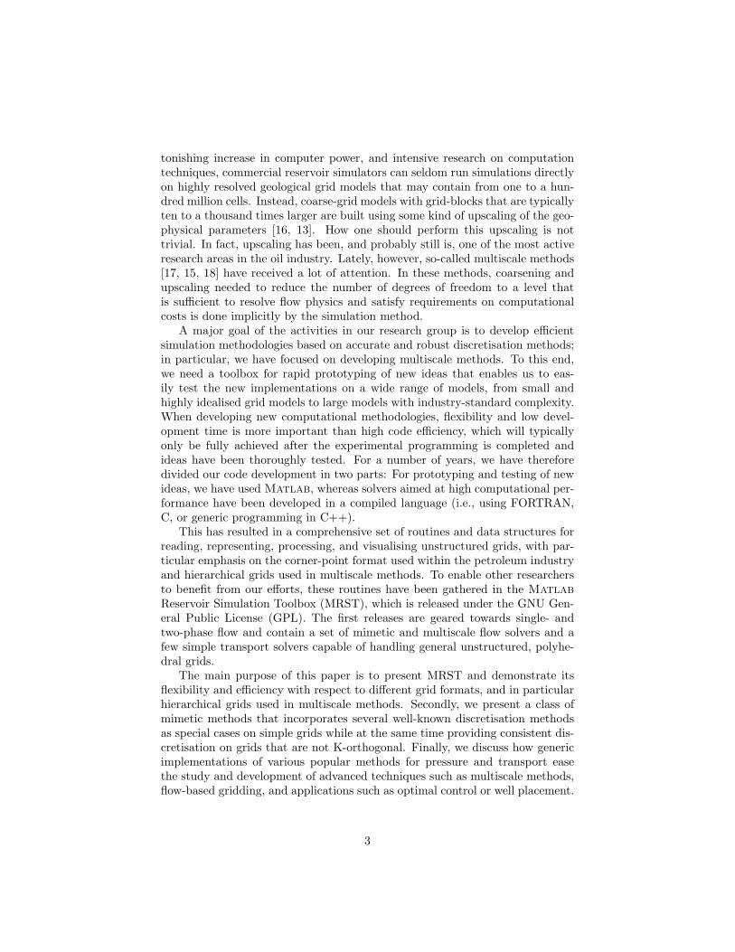
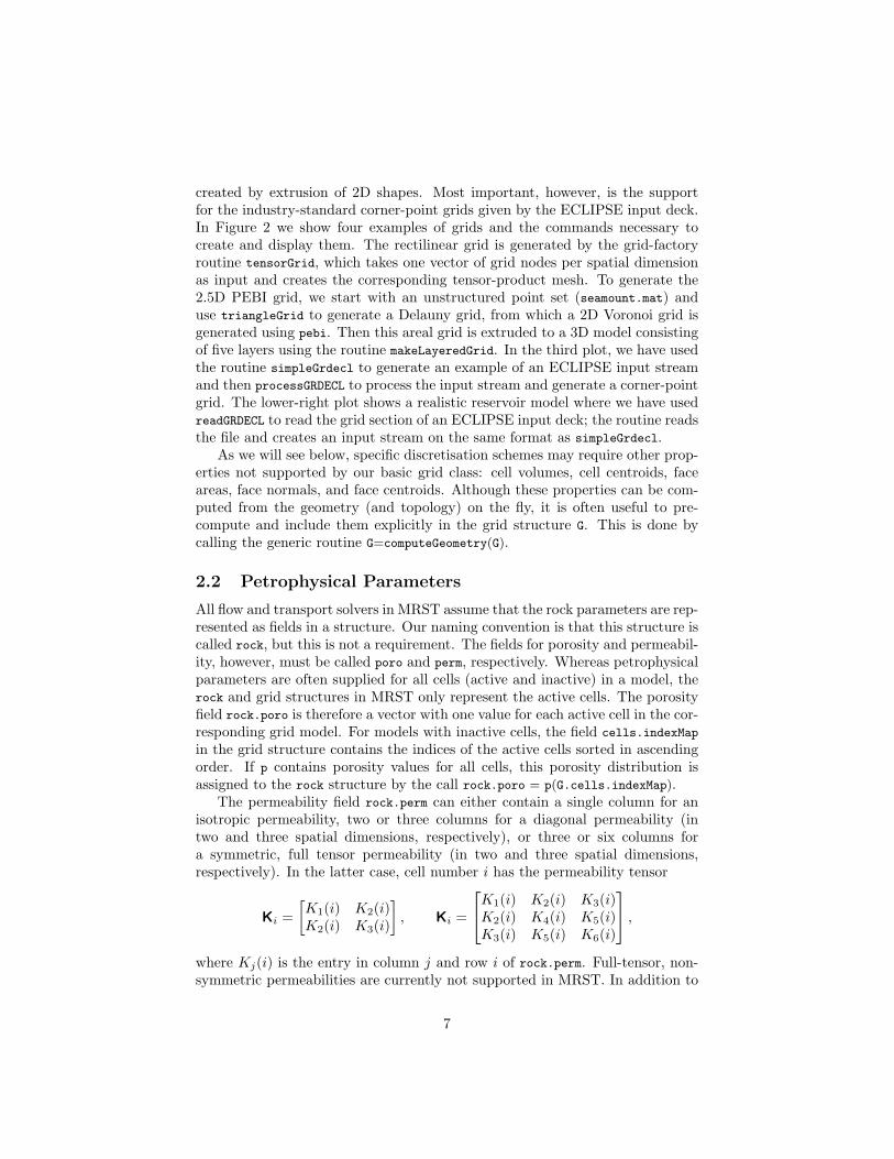
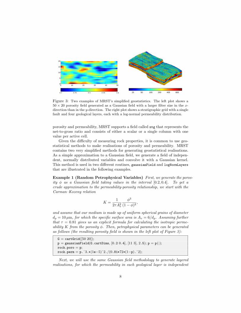
Figure 3: Two examples of MRST’s simplified geostatistics. The left plot shows a50 × 20 porosity field generated as a Gaussian field with a larger filter size in the x-direction than in the y-direction. The right plot shows a stratigraphic grid with a singlefault and four geological layers, each with a log-normal permeability distribution.
porosity and permeability, MRST supports a field called ntg that represents thenet-to-gross ratio and consists of either a scalar or a single column with onevalue per active cell.
Given the difficulty of measuring rock properties, it is common to use geo-statistical methods to make realisations of porosity and permeability. MRSTcontains two very simplified methods for generating geostatistical realisations.As a simple approximation to a Gaussian field, we generate a field of indepen-dent, normally distributed variables and convolve it with a Gaussian kernel.This method is used in two different routines, gaussianField and logNormLayers
that are illustrated in the following examples.
Example 1 (Random Petrophysical Variables) First, we generate the poros-ity φ as a Gaussian field taking values in the interval [0.2, 0.4]. To get acrude approximation to the permeability-porosity relationship, we start with theCarman–Kozeny relation
K =1
2τA2v
φ3
(1− φ)2,
and assume that our medium is made up of uniform spherical grains of diameterdp = 10µm, for which the specific surface area is Av = 6/dp. Assuming furtherthat τ = 0.81 gives us an explicit formula for calculating the isotropic perme-ability K from the porosity φ. Then, petrophysical parameters can be generatedas follows (the resulting porosity field is shown in the left plot of Figure 3):
G = cartGrid([50 20]);p = gaussianField(G.cartDims, [0.2 0.4], [11 3], 2.5); p = p(:);rock.poro = p;rock.perm = p.ˆ3.*(1e−5)ˆ2./(0.81*72*(1−p).ˆ2);
Next, we will use the same Gaussian field methodology to generate layeredrealisations, for which the permeability in each geological layer is independent
8
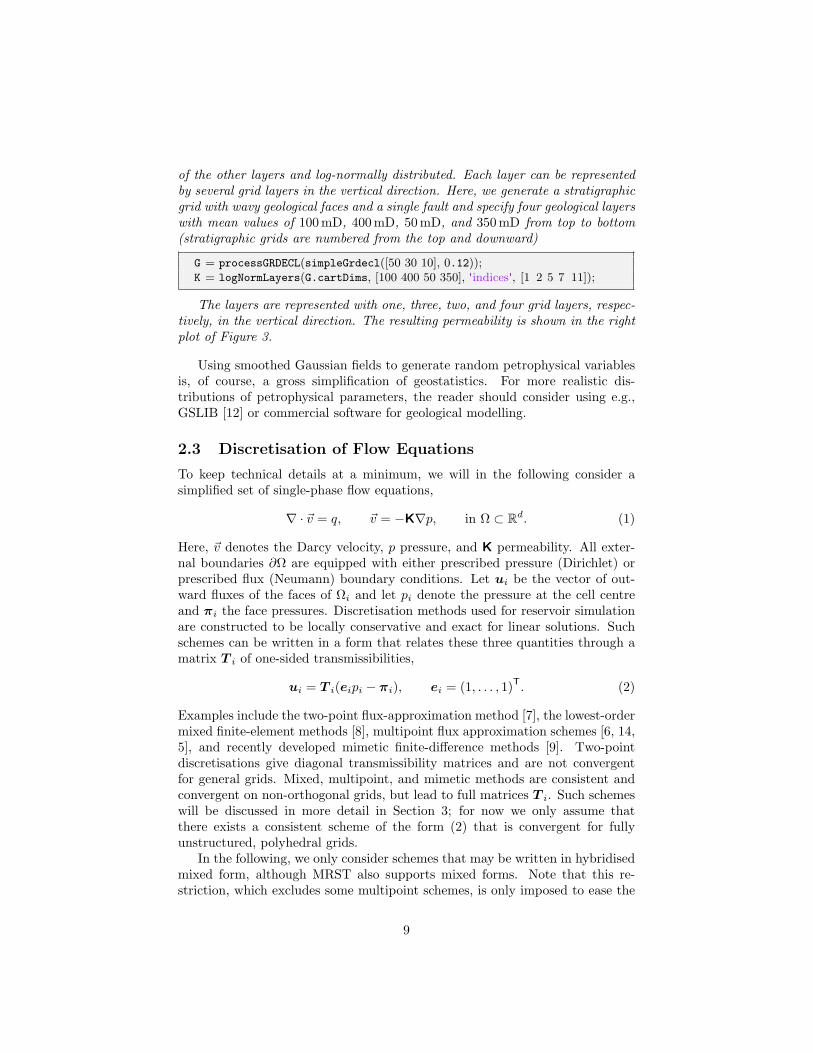
of the other layers and log-normally distributed. Each layer can be representedby several grid layers in the vertical direction. Here, we generate a stratigraphicgrid with wavy geological faces and a single fault and specify four geological layerswith mean values of 100 mD, 400 mD, 50 mD, and 350 mD from top to bottom(stratigraphic grids are numbered from the top and downward)
G = processGRDECL(simpleGrdecl([50 30 10], 0.12));K = logNormLayers(G.cartDims, [100 400 50 350], 'indices', [1 2 5 7 11]);
The layers are represented with one, three, two, and four grid layers, respec-tively, in the vertical direction. The resulting permeability is shown in the rightplot of Figure 3.
Using smoothed Gaussian fields to generate random petrophysical variablesis, of course, a gross simplification of geostatistics. For more realistic dis-tributions of petrophysical parameters, the reader should consider using e.g.,GSLIB [12] or commercial software for geological modelling.
2.3 Discretisation of Flow Equations
To keep technical details at a minimum, we will in the following consider asimplified set of single-phase flow equations,
∇ · ~v = q, ~v = −K∇p, in Ω ⊂ Rd. (1)
Here, ~v denotes the Darcy velocity, p pressure, and K permeability. All exter-nal boundaries ∂Ω are equipped with either prescribed pressure (Dirichlet) orprescribed flux (Neumann) boundary conditions. Let ui be the vector of out-ward fluxes of the faces of Ωi and let pi denote the pressure at the cell centreand πi the face pressures. Discretisation methods used for reservoir simulationare constructed to be locally conservative and exact for linear solutions. Suchschemes can be written in a form that relates these three quantities through amatrix T i of one-sided transmissibilities,
ui = T i(eipi − πi), ei = (1, . . . , 1)T. (2)
Examples include the two-point flux-approximation method [7], the lowest-ordermixed finite-element methods [8], multipoint flux approximation schemes [6, 14,5], and recently developed mimetic finite-difference methods [9]. Two-pointdiscretisations give diagonal transmissibility matrices and are not convergentfor general grids. Mixed, multipoint, and mimetic methods are consistent andconvergent on non-orthogonal grids, but lead to full matrices T i. Such schemeswill be discussed in more detail in Section 3; for now we only assume thatthere exists a consistent scheme of the form (2) that is convergent for fullyunstructured, polyhedral grids.
In the following, we only consider schemes that may be written in hybridisedmixed form, although MRST also supports mixed forms. Note that this re-striction, which excludes some multipoint schemes, is only imposed to ease the
9
presentation and give a uniform formulation of a large class of schemes. Theunderlying principles may be applied to any reasonable scheme. By augmenting(2) with flux and pressure continuity across cell faces, we obtain the followinglinear system [8] B C D
CT 0 0DT 0 0
u−pπ
=
0q0
. (3)
Here, the first row in the block-matrix equation corresponds to Darcy’s law inthe form (2) for all grid cells, the second row corresponds to mass conservationfor all cells, whereas the third row expresses continuity of fluxes for all cell faces.Thus, u denotes the outward face fluxes ordered cell-wise (fluxes over interiorfaces and faults appear twice with opposite signs), p denotes the cell pressures,and π the face pressures. The matrices B and C are block diagonal with eachblock corresponding to a cell. For the two matrices, the i’th blocks are given asT−1i and ei, respectively. Similarly, each column of D corresponds to a unique
face and has one (for boundary faces) or two (for interior faces) unit entriescorresponding to the index(s) of the face in the cell-wise ordering.
The hybrid system (3) can be solved using a Schur-complement method andMatlab’s standard linear solvers or third-party linear system solver softwaresuch as AGMG [29]. A block-wise Gaussian elimination for (3) yields a positive-definite system (the Schur complement) for the face pressures,(
DTB−1D − F TL−1F)π = F TL−1q, (4)
where F = CTB−1D and L = CTB−1C. Given the face pressures, the cellpressures and fluxes can be reconstructed by back-substitution, i.e., solving
Lp = q + Fπ, Bu = Cp−Dπ.
Here, the matrix L is by construction diagonal and computing fluxes is thereforean inexpensive operation. It is also worth noting that we only need B−1 in thesolution procedure above. Many schemes—including the mimetic method, theMPFA-O method, and the standard two-point scheme—yield algebraic approx-imations for the B−1 matrix. Thus, (3) encompasses a family of discretisationschemes whose properties are determined by the choice of B, which we willdiscuss in more detail in Section 3.1.
2.4 Putting it all Together
In this section, we will go through a very simple example to give an overview ofhow to set up and use a discretisation as introduced in the previous section tosolve the single-phase pressure equation
∇ · ~v = q, ~v = −K
µ
[∇p+ ρg∇z
]. (5)
First, we construct a Cartesian grid of size nx × ny × nz cells, where each cellhas dimension 1 × 1 × 1 m and set an isotropic and homogeneous permeabilityof 100 mD, a fluid viscosity of 1 cP, and a fluid density of 1014 kg/m3:
10
nx = 20; ny = 20; nz = 10;G = computeGeometry(cartGrid([nx, ny, nz]));rock.perm = repmat(100 * milli*darcy, [G.cells.num, 1]);fluid = initSingleFluid('mu', 1*centi*poise, 'rho', 1014*kilogram/meterˆ3);gravity reset on
The simplest way to model inflow or outflow from the reservoir is to use a fluidsource/sink. Here, we specify a source with flux rate of 1 m3/day in each gridcell.
c = (nx/2*ny+nx/2 : nx*ny : nx*ny*nz) .';src = addSource([], c, ones(size(c)) ./ day());
Flow solvers in MRST automatically assume no-flow conditions on all outer(and inner) boundaries; other types of boundary conditions need to be specifiedexplicitly. To draw fluid out of the domain, we impose a Dirichlet boundarycondition of p = 10 bar at the global left-hand side of the model.
bc = pside([], G, 'LEFT', 10*barsa());
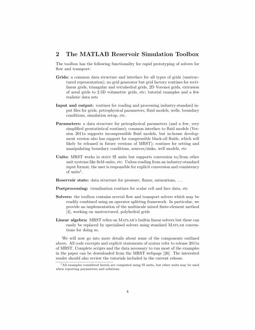
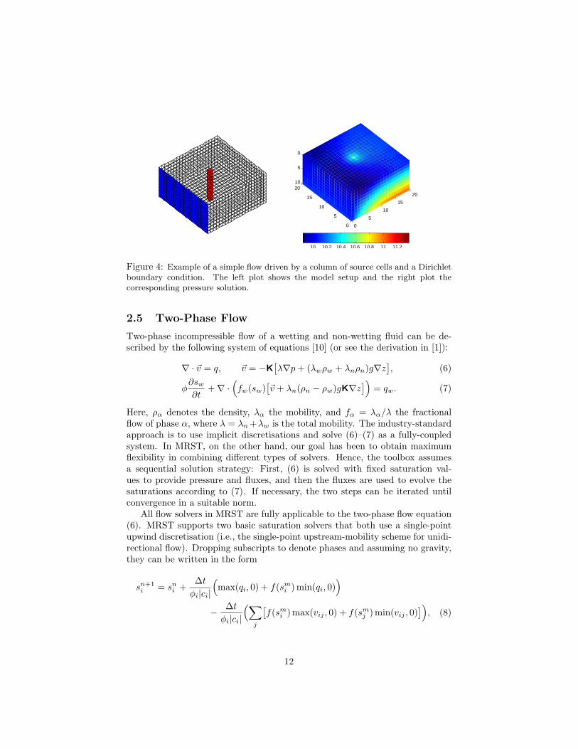
Here, the first argument has been left empty because this is the first bound-ary condition we prescribe. The left plot in Figure 4 shows the placement ofboundary conditions and sources in the computational domain. Next, we con-struct the system components for the hybrid mimetic system (3), with a mimeticdiscretisation, based on input grid and rock properties.
S = computeMimeticIP(G, rock, 'Verbose', true);
Rather than storing B, we store its inverse B−1. Similarly, the C and D blocksare not represented in the S structure; they can easily be formed explicitlywhenever needed, or their action can easily be computed.
Finally, we compute the solution to the flow equation. To this end, we mustfirst create a state object that will be used to hold the solution and then passthis objects and the parameters to the incompressible flow solver.
rSol = initResSol(G, 0);rSol = solveIncompFlow(rSol, G, S, fluid,'src', src, 'bc' , bc);p = convertTo(rSol.pressure(1:G.cells.num), barsa() );
Having computed the solution, we convert the result back to the unit bars. Theright plot in Figure 4 shows the corresponding pressure distribution, where weclearly can see the effects of boundary conditions, source term, and gravity.
The same basic steps can be repeated on (almost) any type of grid; the onlydifference is placing the source terms and how to set the boundary conditions,which will typically be more complicated on a fully unstructured grid. We willcome back with more examples later in the paper, but then we will not explic-itly state all details of the corresponding MRST scripts. Before giving moreexamples, however, we will introduce the multiscale flow solver implemented inMRST.
11
0
5
10
15
20
0
5
10
15
20
0
5
10
10 10.2 10.4 10.6 10.8 11 11.2
Figure 4: Example of a simple flow driven by a column of source cells and a Dirichletboundary condition. The left plot shows the model setup and the right plot thecorresponding pressure solution.
2.5 Two-Phase Flow
Two-phase incompressible flow of a wetting and non-wetting fluid can be de-scribed by the following system of equations [10] (or see the derivation in [1]):
∇ · ~v = q, ~v = −K[λ∇p+ (λwρw + λnρn)g∇z
], (6)
φ∂sw∂t
+∇ ·(fw(sw)
[~v + λn(ρn − ρw)gK∇z
])= qw. (7)
Here, ρα denotes the density, λα the mobility, and fα = λα/λ the fractionalflow of phase α, where λ = λn+λw is the total mobility. The industry-standardapproach is to use implicit discretisations and solve (6)–(7) as a fully-coupledsystem. In MRST, on the other hand, our goal has been to obtain maximumflexibility in combining different types of solvers. Hence, the toolbox assumesa sequential solution strategy: First, (6) is solved with fixed saturation val-ues to provide pressure and fluxes, and then the fluxes are used to evolve thesaturations according to (7). If necessary, the two steps can be iterated untilconvergence in a suitable norm.
All flow solvers in MRST are fully applicable to the two-phase flow equation(6). MRST supports two basic saturation solvers that both use a single-pointupwind discretisation (i.e., the single-point upstream-mobility scheme for unidi-rectional flow). Dropping subscripts to denote phases and assuming no gravity,they can be written in the form
sn+1i = sni +
∆tφi|ci|
(max(qi, 0) + f(smi ) min(qi, 0)
)− ∆tφi|ci|
(∑j
[f(smi ) max(vij , 0) + f(smj ) min(vij , 0)
]), (8)
12
pi πk
Ak~cik
~nk
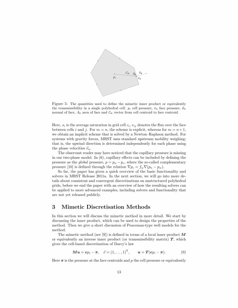
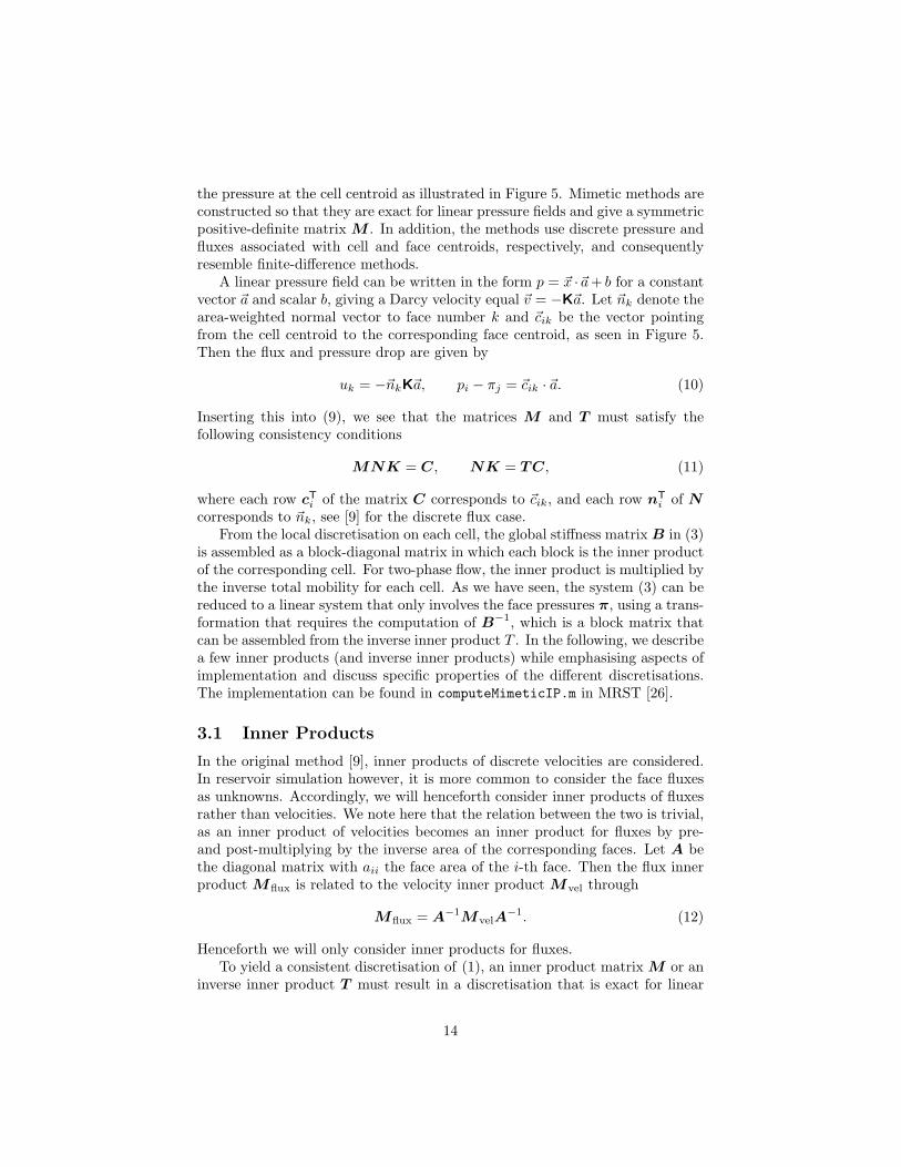
Figure 5: The quantities used to define the mimetic inner product or equivalentlythe transmissibility in a single polyhedral cell: pi cell pressure, πk face pressure, ~nk
normal of face, Ak area of face and ~cik vector from cell centroid to face centroid.
Here, si is the average saturation in grid cell ci, vij denotes the flux over the facebetween cells i and j. For m = n, the scheme is explicit, whereas for m = n+ 1,we obtain an implicit scheme that is solved by a Newton–Raphson method. Forsystems with gravity forces, MRST uses standard upstream mobility weighing;that is, the upwind direction is determined independently for each phase usingthe phase velocities ~vα.
The observant reader may have noticed that the capillary pressure is missingin our two-phase model. In (6), capillary effects can be included by defining thepressure as the global pressure, p = pn− pc, where the so-called complementarypressure [10] is defined through the relation ∇pc = fw∇(pn − pw).
So far, the paper has given a quick overview of the basic functionality andsolvers in MRST Release 2011a. In the next section, we will go into more de-tails about consistent and convergent discretisations on unstructured polyhedralgrids, before we end the paper with an overview of how the resulting solvers canbe applied to more advanced examples, including solvers and functionality thatare not yet released publicly.
3 Mimetic Discretisation Methods
In this section we will discuss the mimetic method in more detail. We start bydiscussing the inner product, which can be used to design the properties of themethod. Then we give a short discussion of Peaceman-type well models for themethod.
The mimetic method (see [9]) is defined in terms of a local inner product Mor equivalently an inverse inner product (or transmissibility matrix) T , whichgives the cell-based discretisation of Darcy’s law
Mu = epi − π, ~e = (1, . . . , 1)T, u = T (epi − π). (9)
Here π is the pressure at the face centroids and p the cell pressure or equivalently
13
the pressure at the cell centroid as illustrated in Figure 5. Mimetic methods areconstructed so that they are exact for linear pressure fields and give a symmetricpositive-definite matrix M . In addition, the methods use discrete pressure andfluxes associated with cell and face centroids, respectively, and consequentlyresemble finite-difference methods.
A linear pressure field can be written in the form p = ~x ·~a+ b for a constantvector ~a and scalar b, giving a Darcy velocity equal ~v = −K~a. Let ~nk denote thearea-weighted normal vector to face number k and ~cik be the vector pointingfrom the cell centroid to the corresponding face centroid, as seen in Figure 5.Then the flux and pressure drop are given by
uk = −~nkK~a, pi − πj = ~cik · ~a. (10)
Inserting this into (9), we see that the matrices M and T must satisfy thefollowing consistency conditions
MNK = C, NK = TC, (11)
where each row cTi of the matrix C corresponds to ~cik, and each row nT
i of Ncorresponds to ~nk, see [9] for the discrete flux case.
From the local discretisation on each cell, the global stiffness matrix B in (3)is assembled as a block-diagonal matrix in which each block is the inner productof the corresponding cell. For two-phase flow, the inner product is multiplied bythe inverse total mobility for each cell. As we have seen, the system (3) can bereduced to a linear system that only involves the face pressures π, using a trans-formation that requires the computation of B−1, which is a block matrix thatcan be assembled from the inverse inner product T . In the following, we describea few inner products (and inverse inner products) while emphasising aspects ofimplementation and discuss specific properties of the different discretisations.The implementation can be found in computeMimeticIP.m in MRST [26].
3.1 Inner Products
In the original method [9], inner products of discrete velocities are considered.In reservoir simulation however, it is more common to consider the face fluxesas unknowns. Accordingly, we will henceforth consider inner products of fluxesrather than velocities. We note here that the relation between the two is trivial,as an inner product of velocities becomes an inner product for fluxes by pre-and post-multiplying by the inverse area of the corresponding faces. Let A bethe diagonal matrix with aii the face area of the i-th face. Then the flux innerproduct Mflux is related to the velocity inner product Mvel through
Mflux = A−1MvelA−1. (12)
Henceforth we will only consider inner products for fluxes.To yield a consistent discretisation of (1), an inner product matrix M or an
inverse inner product T must result in a discretisation that is exact for linear
14
pressures, i.e., fulfils (11). To derive a family of valid solutions, we first observethe following key geometrical property (see [9])
CTN = diag(|Ωi|), (13)
which relates C and N as follows on general polyhedral cells. Multiplying thefirst equation of (11) by K−1CTN , we derive the relation
MN =1|Ωi|
CK−1CTN ,
from which it follows that the family of valid solutions has the form
M =1|Ωi|
CKCT +M2, (14)
in which M2 is a matrix defined such that M is symmetric positive definite andM2N = 0. Any symmetric and positive definite inner product fulfilling theserequirements can be represented in the compact form
M =1|Ωi|
CK−1CT +Q⊥NSMQ⊥N
T, (15)
where Q⊥N is an orthonormal basis for the null space of NT, and SM is anysymmetric, positive-definite matrix. In the code and the following examples,however, we will instead use a null space projection P⊥N = I −QNQN
T, whereQN is a basis for the space spanned by the columns of N . Similarly, the inverseinner products take the form
T =1|Ωi|
NKNT +Q⊥CSQ⊥C
T, (16)
whereQ⊥C is an orthonormal basis for the nullspace ofCT and P⊥C = I−QCQCT
is the corresponding nullspace projection.The matrices M and T in (15) and (16) are evidently symmetric so only an
argument for the positive definiteness is in order. Writing M in (15) as M =M1 +M2, positive semi-definiteness of M1 and M2 imply that M is positivesemi-definite. Let z be an arbitrary non-zero vector which we split (uniquely) asz = Nz + z′ where NTz′ = 0. If z′ = 0, we have zTMz = zTNTM1Nz > 0since CTN has full rank. If z′ 6= 0, we have zTMz = zTM1z + z′TM2z
′ > 0since zTM1z ≥ 0 and z′TM2z
′ > 0. An analogous argument holds for thematrix T .
We will now outline a few specific and valid choices that are implemented inthe basic flow solvers of MRST. We start by considering the one-dimensional casewith the cell [−1, 1] for which N = C = [1,−1]T and Q⊥N = Q⊥C = 1√
2[1, 1]T.
Hence
M =12
[1−1
]1K
[1,−1] +12
[11
]SM [1, 1],
T =12
[1−1
]K [1,−1] +
12
[11
]S [1, 1].
(17)
15
The structure of the inner product should be invariant under scaling of K andthus we can write the inner product as a one-parameter family of the form
M =1
2K
([1 −1−1 1
]+
2t
[1 11 1
]),
T =K
2
([1 −1−1 1
]+t
2
[1 11 1
]).
(18)
In the following, we will use this one-dimensional expression together with trans-formation properties of the inner product to look at the correspondence betweenmimetic, TPFA, and Raviart–Thomas methods.
Two-point type methods. The TPFA method is the gold standard for prac-tical reservoir simulation despite its theoretical shortcomings. Since the TPFAdiscretisation requires a diagonal tensor, it is easily seen from (11) that this isonly possible in the case when the vectors K~ni and ~ci are parallel, i.e., the gridis K-orthogonal. In any case (K-orthogonality or not), we define the diagonalTPFA transmissibility tensor T by
T ii = ~ni ·K~ci/|~ci|2. (19)
This defines the unique TPFA method for K-orthogonal grids3. The extensionto non-orthogonal grids is not unique, and the TPFA method does not givea consistent discretisation in this case. Because of its simplicity, the TPFAmethod is strictly monotone if Tii > 0, which implies that the fluxes form adirected acyclic graph, a property that can be used to accelerate the solution ofthe transport equations considerably, as discussed in [28].
When written in its standard form, the TPFA method is cell-centred andthus less computationally costly than face-centred methods that arise from aconsistent hybrid mimetic formulation. However, since the method is not con-sistent, it will in many cases be necessary to investigate the grid-orientationeffects of the TPFA method before using it for realistic simulations. We there-fore present a mimetic-type discretisation that coincides with the TPFA methodin its region of validity, while at the same time giving a valid mimetic inner prod-uct for all types of grids and permeability tensors. This minimises the need forinvestigating other effects of the TPFA method, such as errors introduced bycorners and well modelling. An advantage of this method compared to using,e.g., an MPFA method is that the implementation is simpler for general unstruc-tured grids. We refer to the corresponding method as IP QTPFA. To derive themethod, we consider a cuboid cell and insert (10) into (9) defined for a singleface to obtain
Tii~ci · ~a = ~niK~a.
3As written, this does not always yield a positive value for the two-point transmissibility.To ensure positive transmissibilities it is normal to define the face centroids as the arithmeticmean of the associated corner-point nodes and the cell centroids as the arithmetic mean of thetop and bottom surface centroids. For most reservoir grids this gives a positive transmissibility.
16
c1
c2
c3
c4
n1 n
2
n3
n4
~c1 + ~c2 = 0, ~c3 + ~c4 = 0
=⇒ Q⊥C =1√2
1 01 00 10 1
~n1 + ~n2 = 0, ~n3 + ~n4 = 0
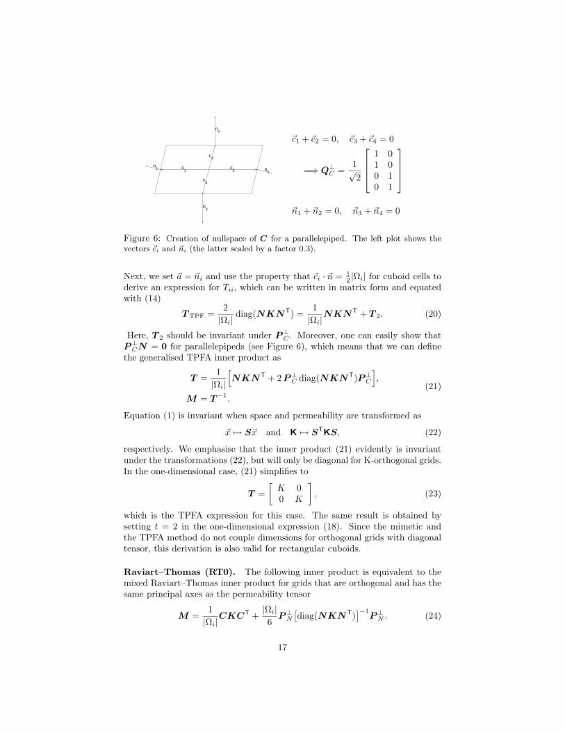
Figure 6: Creation of nullspace of C for a parallelepiped. The left plot shows thevectors ~ci and ~ni (the latter scaled by a factor 0.3).
Next, we set ~a = ~ni and use the property that ~ci · ~n = 12 |Ωi| for cuboid cells to
derive an expression for Tii, which can be written in matrix form and equatedwith (14)
TTPF =2|Ωi|
diag(NKNT) =1|Ωi|
NKNT + T 2. (20)
Here, T 2 should be invariant under P⊥C . Moreover, one can easily show thatP⊥CN = 0 for parallelepipeds (see Figure 6), which means that we can definethe generalised TPFA inner product as
T =1|Ωi|
[NKNT + 2P⊥C diag(NKNT)P⊥C
],
M = T−1.
(21)
Equation (1) is invariant when space and permeability are transformed as
~x 7→ S~x and K 7→ STKS, (22)
respectively. We emphasise that the inner product (21) evidently is invariantunder the transformations (22), but will only be diagonal for K-orthogonal grids.In the one-dimensional case, (21) simplifies to
T =[K 00 K
], (23)
which is the TPFA expression for this case. The same result is obtained bysetting t = 2 in the one-dimensional expression (18). Since the mimetic andthe TPFA method do not couple dimensions for orthogonal grids with diagonaltensor, this derivation is also valid for rectangular cuboids.
Raviart–Thomas (RT0). The following inner product is equivalent to themixed Raviart–Thomas inner product for grids that are orthogonal and has thesame principal axes as the permeability tensor
M =1|Ωi|
CKCT +|Ωi|6P⊥N
[diag(NKNT)
]−1P⊥N . (24)
17
This can be verified by a direct calculation for the one-dimensional case, whichreduces to
M =1K
[2/3 −1/3−1/3 2/3
], (25)
which coincides with (18) for t = 6. The fact that this inner product does notcouple different directions for orthogonal grids and diagonal tensors implies that(24) is also equal to the lowest-order Raviart–Thomas (RT0) method on (rectan-gular) cuboids. We refer to this inner product as ‘IP QRT’. The correspondingquasi-inverse, which is the exact inverse for orthogonal grids, reads
T =1|Ωi|
[NKNT + 6P⊥C diag(NKNT)P⊥C
]. (26)
This inner product will also, by the transformation property, be equal to theRaviart–Thomas formulation for all cases that can be transformed to the abovecase by an affine transformation of the form (22). Using a mimetic inner productwhich is simpler to calculate and equal to the mixed RT0 inner product for allgrid cells is not possible because of the need to integrate the nonlinear functionintroduced by the determinant of the Jacobian of the mapping from the gridcell to the unit cell where the RT0 basis functions are defined.
Local-flux mimetic MPFA. In addition to the above methods, which areall based on the assumption of a positive-definite inner product and exactnessfor linear flow, the MPFA method can be formulated as a mimetic method.This was first done by [21, 24] and is called the local-flux mimetic formulationof the MPFA method. In this case, all faces of a cell are such that each corneris associated with d unique faces, where d is the dimension. The inner productof the local-flux mimetic method gives exact result for linear flow and is blockdiagonal with respect to the faces corresponding to each corner of the cell, but itis not symmetric. The block-diagonal property makes it possible to reduce thesystem into a cell-centred discretisation for the cell pressures. This naturallyleads to a method for calculating the MPFA transmissibilities. The crucial pointis to have the corner geometry in the grid structure and handle the problemswith corners which do not have three unique half faces associated. Currentlythe MPFA-O method is formulated in such a way [21] and work has been donefor the MPFA-L method, but in this case the inner product will vary over thedifferent corners. Our implementation of MPFA is based upon a combinationof Matlab and C and is therefore available as an add-on module to MRST.
Parametric family. We notice that the (inverse) inner products IP QTPFAin (21) and IP QRT in (26) differ only by a constant in front of the regularisationpart (the second term). Both methods belong to a family whose inverse innerproduct can be written in the form
T =1|Ωi|
[NKNT + tP⊥C diag(NKNT)P⊥C
]M = T−1,
(27)
18
in which t is a parameter that can be varied continuously from zero to infinity. InMRST, this family of inner products is called ‘IP QFAMILY’ and the parametert is supplied in a separate option
S = computeMimeticIP(G, rock, 'Verbose', true,...'InnerProduct', ' ip qfamily ' , 'qparam', t);
IP SIMPLE. For historical reasons, the default inner product used in MRSTreads
Q = orth(A−1N)
M =1|Ωi|
CK−1CT +d|Ωi|
6 tr(K)A−1(I −QQT)A−1
(28)
with the approximate inverse
Q = orth(AC)
T =1|Ωi|
[NKNT +
6d
tr(K)A(I −QQT)A].
(29)
This inner product was used in [4] inspired by [9] and was chosen to resemble themixed Raviart–Thomas inner product (they are equal for scalar permeability onorthogonal grids, which can be verified by inspection. Since this inner productis based on velocities, it involves pre- and post-multiplication of (inverse) faceareas, and it might not be obvious that it fits into the formulations (15)–(16).However, after a small computation one is convinced that the second part of(15) is invariant under multiplication by P⊥N so its eigenspace correspondingto the nonzero eigenvalues must be equal to the nullspace of NT. A similarargument holds for the inverse inner product.
Example 2 (Grid-Orientation Effects and Monotonicity) It is well knownthat two-point approximations are convergent only in the special case of K-orthogonal grids. Mimetic and multipoint schemes, on the other hand, areconstructed to be consistent and convergent for rough grids and full-tensor per-meabilities, but may suffer from pressure oscillations for full-tensor permeabil-ities and large anisotropy ratios and/or high aspect ratio grids. In this exam-ple, we use one of the example grids supplied with MRST to illustrate thesetwo observations. The routine twister normalises all coordinates in a rec-tilinear grid to the interval [0, 1], then perturbs all interior points by adding0.03 sin(πx) sin(3π(y−1/2)) to the x-coordinates and subtracting the same valuefrom the y-coordinate before transforming back to the original domain. This cre-ates a non-orthogonal, but smoothly varying, logically Cartesian grid.
To investigate grid-orientation effects, we impose a permeability tensor withanisotropy ratio 1 : 1000 aligned with the x-axis and compute the flow resultingfrom a prescribed horizontal pressure drop and no-flow conditions on the top andbottom boundaries. Figure 7 shows pressure computed on a 100 × 100 grid by
19
0 50 1000
20
40
60
80
100TPFA
0 50 1000
20
40
60
80
100mimetic
0 50 1000
20
40
60
80
100MPFA
0 50 1000
20
40
60
80
100
x0 50 100
0
20
40
60
80
100
x0 50 100
0
20
40
60
80
100
x
20
30
40
50
60
70
80
90
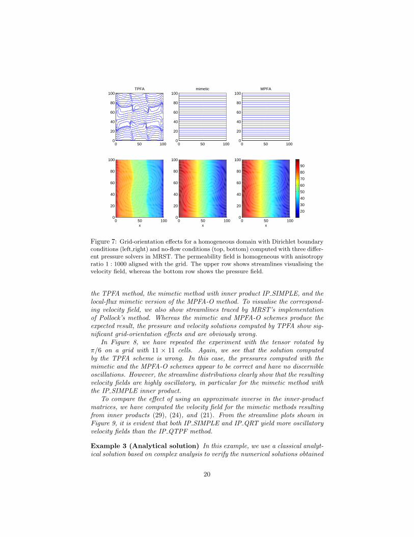
Figure 7: Grid-orientation effects for a homogeneous domain with Dirichlet boundaryconditions (left,right) and no-flow conditions (top, bottom) computed with three differ-ent pressure solvers in MRST. The permeability field is homogeneous with anisotropyratio 1 : 1000 aligned with the grid. The upper row shows streamlines visualising thevelocity field, whereas the bottom row shows the pressure field.
the TPFA method, the mimetic method with inner product IP SIMPLE, and thelocal-flux mimetic version of the MPFA-O method. To visualise the correspond-ing velocity field, we also show streamlines traced by MRST’s implementationof Pollock’s method. Whereas the mimetic and MPFA-O schemes produce theexpected result, the pressure and velocity solutions computed by TPFA show sig-nificant grid-orientation effects and are obviously wrong.
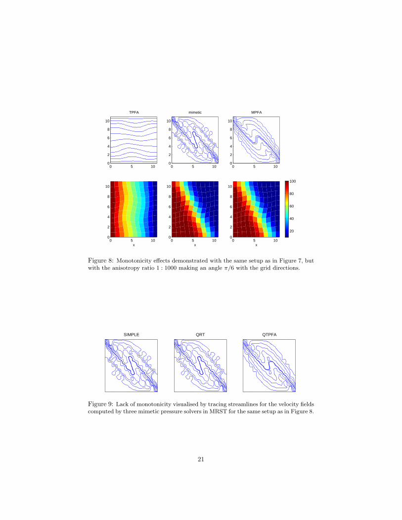
In Figure 8, we have repeated the experiment with the tensor rotated byπ/6 on a grid with 11 × 11 cells. Again, we see that the solution computedby the TPFA scheme is wrong. In this case, the pressures computed with themimetic and the MPFA-O schemes appear to be correct and have no discernibleoscillations. However, the streamline distributions clearly show that the resultingvelocity fields are highly oscillatory, in particular for the mimetic method withthe IP SIMPLE inner product.
To compare the effect of using an approximate inverse in the inner-productmatrices, we have computed the velocity field for the mimetic methods resultingfrom inner products (29), (24), and (21). From the streamline plots shown inFigure 9, it is evident that both IP SIMPLE and IP QRT yield more oscillatoryvelocity fields than the IP QTPF method.
Example 3 (Analytical solution) In this example, we use a classical analyt-ical solution based on complex analysis to verify the numerical solutions obtained
20
0 5 100
2
4
6
8
10
TPFA
0 5 100
2
4
6
8
10
mimetic
0 5 100
2
4
6
8
10
MPFA
0 5 100
2
4
6
8
10
x0 5 10
0
2
4
6
8
10
x0 5 10
0
2
4
6
8
10
x
20
40
60
80
100
Figure 8: Monotonicity effects demonstrated with the same setup as in Figure 7, butwith the anisotropy ratio 1 : 1000 making an angle π/6 with the grid directions.
SIMPLE QRT QTPFA
Figure 9: Lack of monotonicity visualised by tracing streamlines for the velocity fieldscomputed by three mimetic pressure solvers in MRST for the same setup as in Figure 8.
21
by MRST. A standard method to construct analytical solutions to the Laplacianequation in 2D is to write the unknown as the real or imaginary part of an com-plex analytic function f(z). We choose the function f(z) = (z + 1
2z2) and set
our analytical solution to be pa(x, y) = If(x + iy) = y + xy. As our computa-tional domain, we choose a 2D triangular grid generated from the seamount.mat
data set (see e.g., the upper-left plot in Figure 2) and its dual Voronoi grid, bothcentred at the origin. By prescribing pa(x, y) along the boundary, we obtain aDirichlet problem with known solution.
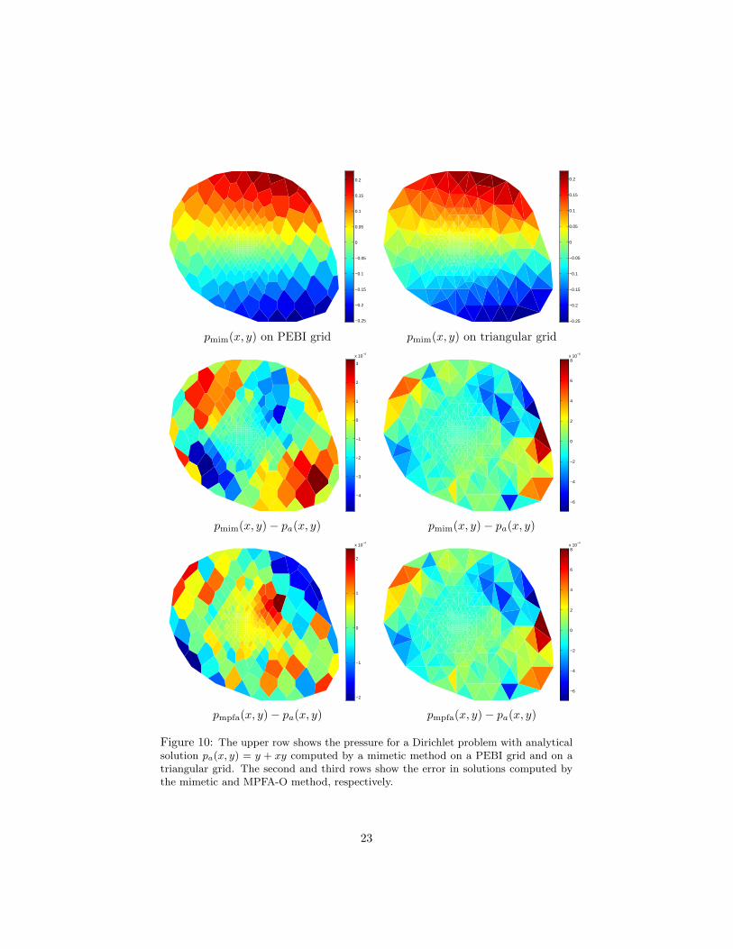
To compute numerical approximations to pa(x, y) we use the MPFA-O schemeand the mimetic method with inner product ’IP SIMPLE’. Figure 10 shows theapproximate solutions and the discrepancy from the analytical solution at thecell centres for both grids. For the triangular grid, the two methods produce theexact same result because all mimetic methods with a symmetric inner productare identical for cell and face pressures on triangular grids. On the Voronoigrid, the mimetic method is slightly more accurate than the MPFA-O methodand both methods have lower errors than on the triangular grid.
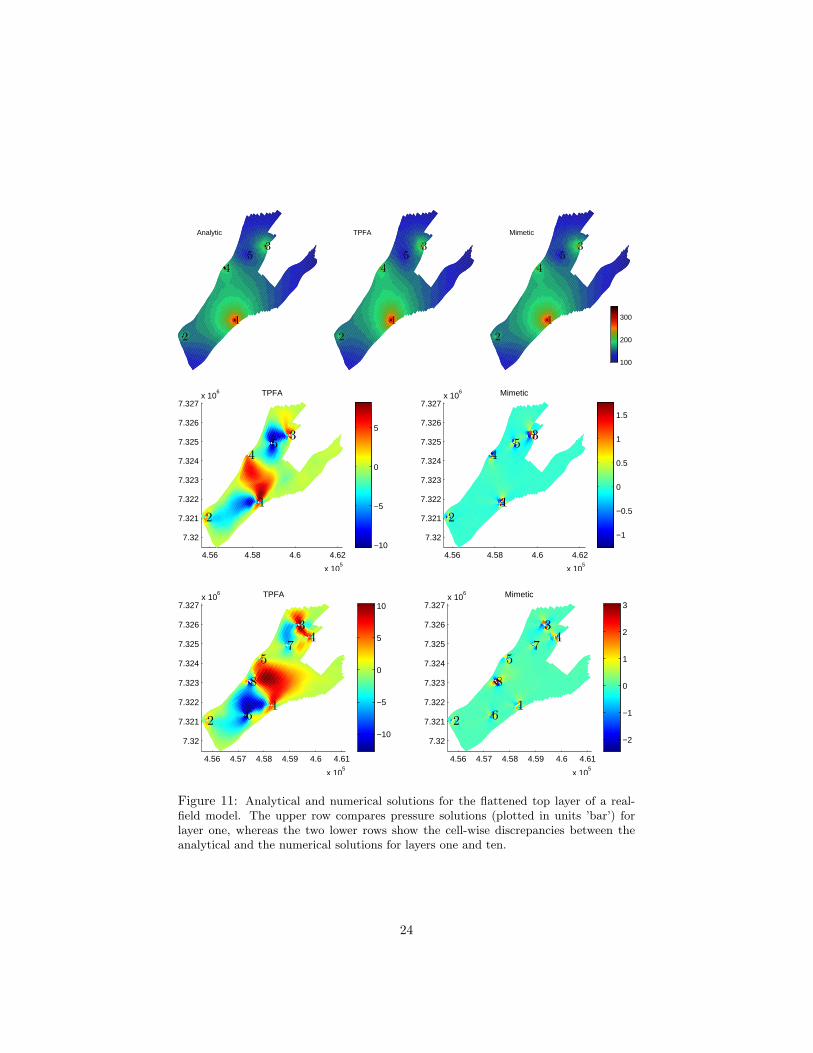
Example 4 (Real-Field Model) In this example, we consider two syntheticmodels derived from the 3D simulation model of a reservoir from offshore Nor-way. The original model is given as a 46× 112× 22 logically Cartesian corner-point grid with 44,915 active cells. To assess grid-orientation effects introducedby different inner products, we consider two single layers (layer one and tenfrom the top of the model), which we flatten and modify so that the thickness isconstant and all pillars in the corner-point description are vertical. Well posi-tions are assigned by keeping one perforation for each of the original wells. Let(xi, yi), i = 1, . . . , n denote the resulting well positions and qi the well rates. Ifwe model each well as a logarithmic singularity along a vertical line at (xi, yi),the corresponding analytical solution to (1) in an infinite domain with constantpermeability K is given by
p(x, y, z) =n∑i=1
qi2πK
ln(√
(x− xi)2 + (y − yi)2). (30)
To generate a representative analytical solution, we set K = 500 mD andprescribe (30) along the outer lateral boundary of each model. In Figure 11,we compare this analytical solution with numerical solution computed by theTPFA method and the mimetic IP QRT method for the first layer. Whereasthe mimetic solution shows good correspondence with the analytical solution,the TPFA solution exhibits large grid-orientation effects, which are particularlyevident between wells one and four and in the region below well two. With theconsistent mimetic scheme, the error is localised around the wells, whereas it isup to 10 % and distributed all over the reservoir for the TPFA method. (Thefull 3D model has a much rougher geometry that contains pinch-outs, slopingfaults, and eroded layers, which all will contributed to larger grid-orientationeffects for inconsistent methods). In a real simulation, a good well model e.g.,as discussed in the next section) can correct for errors in the vicinity of the well,but not global errors as in the inconsistent TPFA method.
22
−0.25
−0.2
−0.15
−0.1
−0.05
0
0.05
0.1
0.15
0.2
−0.25
−0.2
−0.15
−0.1
−0.05
0
0.05
0.1
0.15
0.2
pmim(x, y) on PEBI grid pmim(x, y) on triangular grid
−4
−3
−2
−1
0
1
2
3
x 10−4
−6
−4
−2
0
2
4
6
8x 10
−4
pmim(x, y)− pa(x, y) pmim(x, y)− pa(x, y)
−2
−1
0
1
2
x 10−4
−6
−4
−2
0
2
4
6
8x 10
−4
pmpfa(x, y)− pa(x, y) pmpfa(x, y)− pa(x, y)
Figure 10: The upper row shows the pressure for a Dirichlet problem with analyticalsolution pa(x, y) = y + xy computed by a mimetic method on a PEBI grid and on atriangular grid. The second and third rows show the error in solutions computed bythe mimetic and MPFA-O method, respectively.
23
35
1
4
Analytic
2
35
1
4
TPFA
2
35
1
4
Mimetic
2
100
200
300
4.56 4.58 4.6 4.62
x 105
7.32
7.321
7.322
7.323
7.324
7.325
7.326
7.327x 10
6
3
TPFA
5
1
4
2
−10
−5
0
5
4.56 4.58 4.6 4.62
x 105
7.32
7.321
7.322
7.323
7.324
7.325
7.326
7.327x 10
6
3
Mimetic
5
1
4
2
−1
−0.5
0
0.5
1
1.5
4.56 4.57 4.58 4.59 4.6 4.61
x 105
7.32
7.321
7.322
7.323
7.324
7.325
7.326
7.327x 10
6
43
7
TPFA
1
5
8
62
−10
−5
0
5
10
4.56 4.57 4.58 4.59 4.6 4.61
x 105
7.32
7.321
7.322
7.323
7.324
7.325
7.326
7.327x 10
6
43
7
Mimetic
1
5
8
62
−2
−1
0
1
2
3
Figure 11: Analytical and numerical solutions for the flattened top layer of a real-field model. The upper row compares pressure solutions (plotted in units ’bar’) forlayer one, whereas the two lower rows show the cell-wise discrepancies between theanalytical and the numerical solutions for layers one and ten.
24
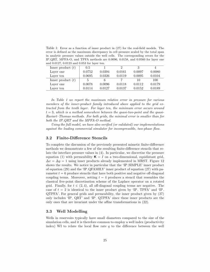
Table 1: Error as a function of inner product in (27) for the real-field models. Theerror is defined as the maximum discrepancy in cell pressure scaled by the total spanin analytic pressure values outside the well cells. The corresponding errors for theIP QRT, MPFA-O, and TPFA methods are 0.0096, 0.0158, and 0.0560 for layer oneand 0.0127, 0.0123 and 0.053 for layer ten.
Inner product (t) 0.5 1 2 3 4Layer one 0.0752 0.0394 0.0161 0.0097 0.0080Layer ten 0.0695 0.0326 0.0119 0.0095 0.0104Inner product (t) 5 6 7 10 100Layer one 0.0078 0.0096 0.0118 0.0112 0.0179Layer ten 0.0114 0.0127 0.0137 0.0152 0.0189
In Table 1 we report the maximum relative error in pressure for variousmembers of the inner-product family introduced above applied to the grid ex-tracted from the tenth layer. For layer ten, the minimum error occurs aroundt = 3, which is a method somewhere between the quasi-two-point and the quasi-Raviart–Thomas methods. For both grids, the minimal error is smaller than forboth the IP QRT and the MPFA-O method.
Using the full model, we have also verified (or validated) our implementationsagainst the leading commercial simulator for incompressible, two-phase flow.
3.2 Finite-Difference Stencils
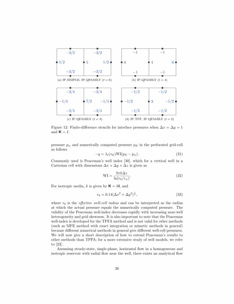
To complete the discussion of the previously presented mimetic finite-differencemethods we demonstrate a few of the resulting finite-difference stencils that re-late the interface pressure values in (4). In particular, we discretise the pressureequation (1) with permeability K = I on a two-dimensional, equidistant grid,∆x = ∆y = 1 using inner products already implemented in MRST. Figure 12shows the results. We notice in particular that the ‘IP SIMPLE’ inner productof equation (29) and the ‘IP QFAMILY’ inner product of equation (27) with pa-rameter t = 6 produce stencils that have both positive and negative off-diagonalcoupling terms. Moreover, setting t = 4 produces a stencil that resembles theclassical five-point discretisation scheme of the Laplace operator on a rotatedgrid. Finally, for t ∈ (2, 4), all off-diagonal coupling terms are negative. Thecase of t = 2 is identical to the inner product given by ‘IP TPFA’ and ‘IPQTPFA’. For general grids and permeability, the inner product given by (27)only includes ‘IP QRT’ and ‘IP QTPFA’ since these inner products are theonly ones that are invariant under the affine transformations in (22).
3.3 Well Modelling
Wells in reservoirs typically have small diameters compared to the size of thesimulation cells, and it is therefore common to employ a well index (productivityindex) WI to relate the local flow rate q to the difference between the well
25
1/2 5 1/2
−3/2 −3/2
−3/2 −3/2
(a) IP SIMPLE, IP QFAMILY (t = 6)
0 4 0
−1 −1
−1 −1
(b) IP QFAMILY (t = 4)
−1/4 7/2 −1/4
−3/4 −3/4
−3/4 −3/4
(c) IP QFAMILY (t = 3)
−1/2 3 −1/2
−1/2 −1/2
−1/2 −1/2
(d) IP TPF, IP QFAMILY (t = 2)
Figure 12: Finite-difference stencils for interface pressures when ∆x = ∆y = 1and K = I.
pressure pw and numerically computed pressure pE in the perforated grid-cellas follows
−q = λt(sE)WI(pE − pw). (31)
Commonly used is Peaceman’s well index [30], which for a vertical well in aCartesian cell with dimensions ∆x×∆y ×∆z is given as
WI =2πk∆z
ln(r0/rw). (32)
For isotropic media, k is given by K = kI, and
r0 = 0.14(∆x2 + ∆y2)12 , (33)
where r0 is the effective well-cell radius and can be interpreted as the radiusat which the actual pressure equals the numerically computed pressure. Thevalidity of the Peaceman well-index decreases rapidly with increasing near-wellheterogeneity and grid skewness. It is also important to note that the Peacemanwell-index is developed for the TPFA method and is not valid for other methods(such as MFE method with exact integration or mimetic methods in general)because different numerical methods in general give different well-cell pressures.We will now give a short description of how to extend Peaceman’s results toother methods than TPFA; for a more extensive study of well models, we referto [23].
Assuming steady-state, single-phase, horizontal flow in a homogeneous andisotropic reservoir with radial flow near the well, there exists an analytical flow
26
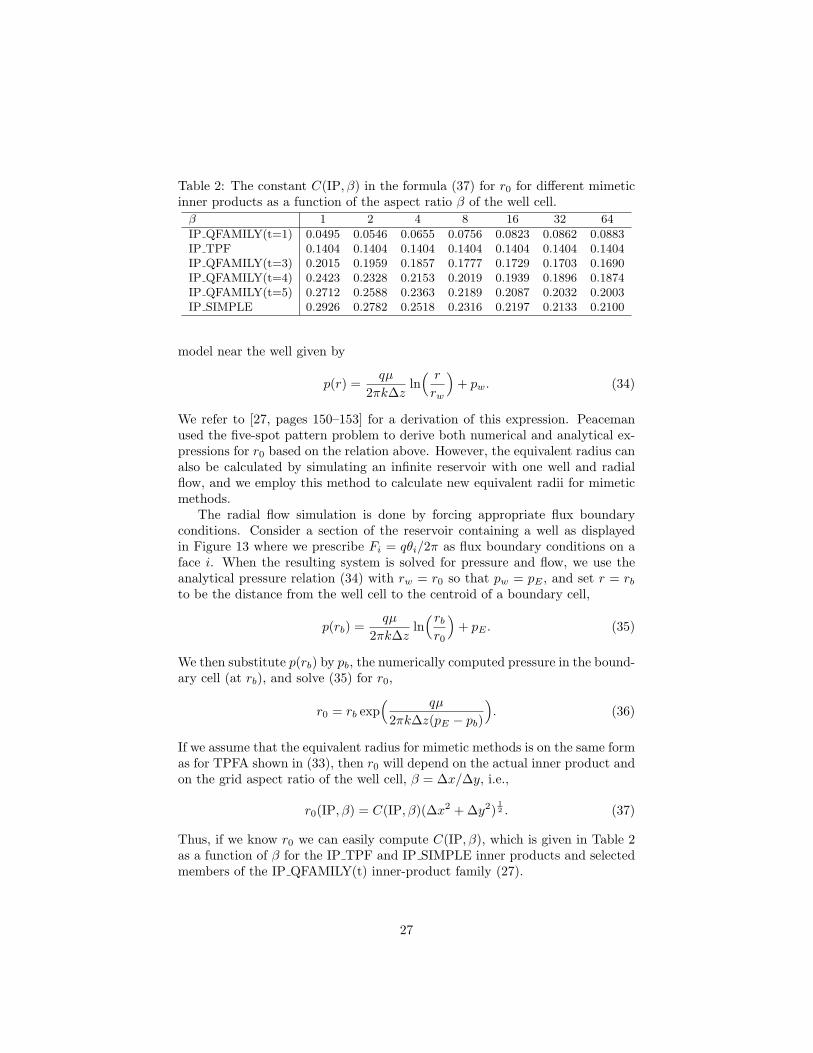
Table 2: The constant C(IP, β) in the formula (37) for r0 for different mimeticinner products as a function of the aspect ratio β of the well cell.β 1 2 4 8 16 32 64
IP QFAMILY(t=1) 0.0495 0.0546 0.0655 0.0756 0.0823 0.0862 0.0883IP TPF 0.1404 0.1404 0.1404 0.1404 0.1404 0.1404 0.1404IP QFAMILY(t=3) 0.2015 0.1959 0.1857 0.1777 0.1729 0.1703 0.1690IP QFAMILY(t=4) 0.2423 0.2328 0.2153 0.2019 0.1939 0.1896 0.1874IP QFAMILY(t=5) 0.2712 0.2588 0.2363 0.2189 0.2087 0.2032 0.2003IP SIMPLE 0.2926 0.2782 0.2518 0.2316 0.2197 0.2133 0.2100
model near the well given by
p(r) =qµ
2πk∆zln( r
rw
)+ pw. (34)
We refer to [27, pages 150–153] for a derivation of this expression. Peacemanused the five-spot pattern problem to derive both numerical and analytical ex-pressions for r0 based on the relation above. However, the equivalent radius canalso be calculated by simulating an infinite reservoir with one well and radialflow, and we employ this method to calculate new equivalent radii for mimeticmethods.
The radial flow simulation is done by forcing appropriate flux boundaryconditions. Consider a section of the reservoir containing a well as displayedin Figure 13 where we prescribe Fi = qθi/2π as flux boundary conditions on aface i. When the resulting system is solved for pressure and flow, we use theanalytical pressure relation (34) with rw = r0 so that pw = pE , and set r = rbto be the distance from the well cell to the centroid of a boundary cell,
p(rb) =qµ
2πk∆zln( rbr0
)+ pE . (35)
We then substitute p(rb) by pb, the numerically computed pressure in the bound-ary cell (at rb), and solve (35) for r0,
r0 = rb exp( qµ
2πk∆z(pE − pb)
). (36)
If we assume that the equivalent radius for mimetic methods is on the same formas for TPFA shown in (33), then r0 will depend on the actual inner product andon the grid aspect ratio of the well cell, β = ∆x/∆y, i.e.,
r0(IP, β) = C(IP, β)(∆x2 + ∆y2)12 . (37)
Thus, if we know r0 we can easily compute C(IP, β), which is given in Table 2as a function of β for the IP TPF and IP SIMPLE inner products and selectedmembers of the IP QFAMILY(t) inner-product family (27).
27
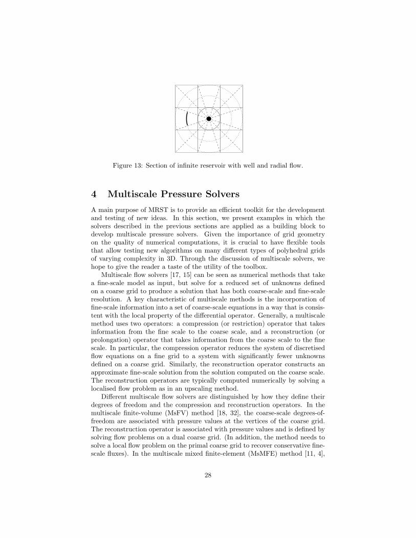
Figure 13: Section of infinite reservoir with well and radial flow.
4 Multiscale Pressure Solvers
A main purpose of MRST is to provide an efficient toolkit for the developmentand testing of new ideas. In this section, we present examples in which thesolvers described in the previous sections are applied as a building block todevelop multiscale pressure solvers. Given the importance of grid geometryon the quality of numerical computations, it is crucial to have flexible toolsthat allow testing new algorithms on many different types of polyhedral gridsof varying complexity in 3D. Through the discussion of multiscale solvers, wehope to give the reader a taste of the utility of the toolbox.
Multiscale flow solvers [17, 15] can be seen as numerical methods that takea fine-scale model as input, but solve for a reduced set of unknowns definedon a coarse grid to produce a solution that has both coarse-scale and fine-scaleresolution. A key characteristic of multiscale methods is the incorporation offine-scale information into a set of coarse-scale equations in a way that is consis-tent with the local property of the differential operator. Generally, a multiscalemethod uses two operators: a compression (or restriction) operator that takesinformation from the fine scale to the coarse scale, and a reconstruction (orprolongation) operator that takes information from the coarse scale to the finescale. In particular, the compression operator reduces the system of discretisedflow equations on a fine grid to a system with significantly fewer unknownsdefined on a coarse grid. Similarly, the reconstruction operator constructs anapproximate fine-scale solution from the solution computed on the coarse scale.The reconstruction operators are typically computed numerically by solving alocalised flow problem as in an upscaling method.
Different multiscale flow solvers are distinguished by how they define theirdegrees of freedom and the compression and reconstruction operators. In themultiscale finite-volume (MsFV) method [18, 32], the coarse-scale degrees-of-freedom are associated with pressure values at the vertices of the coarse grid.The reconstruction operator is associated with pressure values and is defined bysolving flow problems on a dual coarse grid. (In addition, the method needs tosolve a local flow problem on the primal coarse grid to recover conservative fine-scale fluxes). In the multiscale mixed finite-element (MsMFE) method [11, 4],
28
the coarse-scale degrees-of-freedom are associated with faces in the coarse grid(coarse-grid fluxes) and the reconstruction operator is associated with the fluxesand is defined by solving flow problems on a primal coarse grid. In the following,we will present the MsMFE method in more detail. To this end, we will use afinite-element formulation, but the resulting discrete method will have all thecharacteristics of a (mass-conservative) finite-volume method.
The multiscale method implemented in MRST is based on a hierarchicaltwo-level grid in which the blocks Ωi in the coarse simulation grid consist of aconnected set of cells from the underlying fine grid, on which the full heterogene-ity is represented. In its simplest form, the approximation space consists of aconstant approximation of the pressure inside each coarse block and a set of ve-locity basis functions associated with each interface between two coarse blocks.Consider two neighbouring blocks Ωi and Ωj , and let Ωij be a neighbourhoodcontaining Ωi and Ωj . The basis functions ~ψij are constructed by solving
~ψij = −K∇pij , ∇ · ~ψij =
wi(x), if x ∈ Ωi,−wj(x), if x ∈ Ωj ,
0, otherwise,(38)
in Ωij with ~ψij ·~n = 0 on ∂Ωij . If Ωij 6= Ωi∪Ωj , we say that the basis function iscomputed using overlap or oversampling. The purpose of the weighting functionwi(x) is to distribute the divergence of the velocity, ∇ · ~v, over the block andproduce a flow with unit flux over the interface ∂Ωi ∩ ∂Ωj , and the functionis therefore normalised such that its integral over Ωi equals one. Alternatively,the method can be formulated on a single grid block Ωi by specifying a fluxdistribution (with unit average) on one face and no-flow condition on the otherfaces, see [2] for more details. In either case, the multiscale basis functions—represented as vectors Ψij of fluxes—are then collected as columns in a matrixΨ, which will be our reconstruction operator for fine-scale fluxes. To definethe compression operator, we introduce two prolongation operators I and Jfrom blocks to cells and from coarse interfaces to fine faces, respectively. Theoperator I is defined such that element ij equals one if block number j containscell number i and zero otherwise; J is defined analogously. The transposed ofthese operators will thus correspond to the sum over all fine cells of a coarse blockand all fine-cell faces that are part of the faces of the coarse blocks. Applyingthese compression operators and ΨT to the fine-scale system, we obtain thefollowing global coarse-scale system ΨTBΨ ΨTCI ΨTDJ
ITCTΨ 0 0J TDTΨ 0 0
uc
−pcπc
=
0ITq
0
. (39)
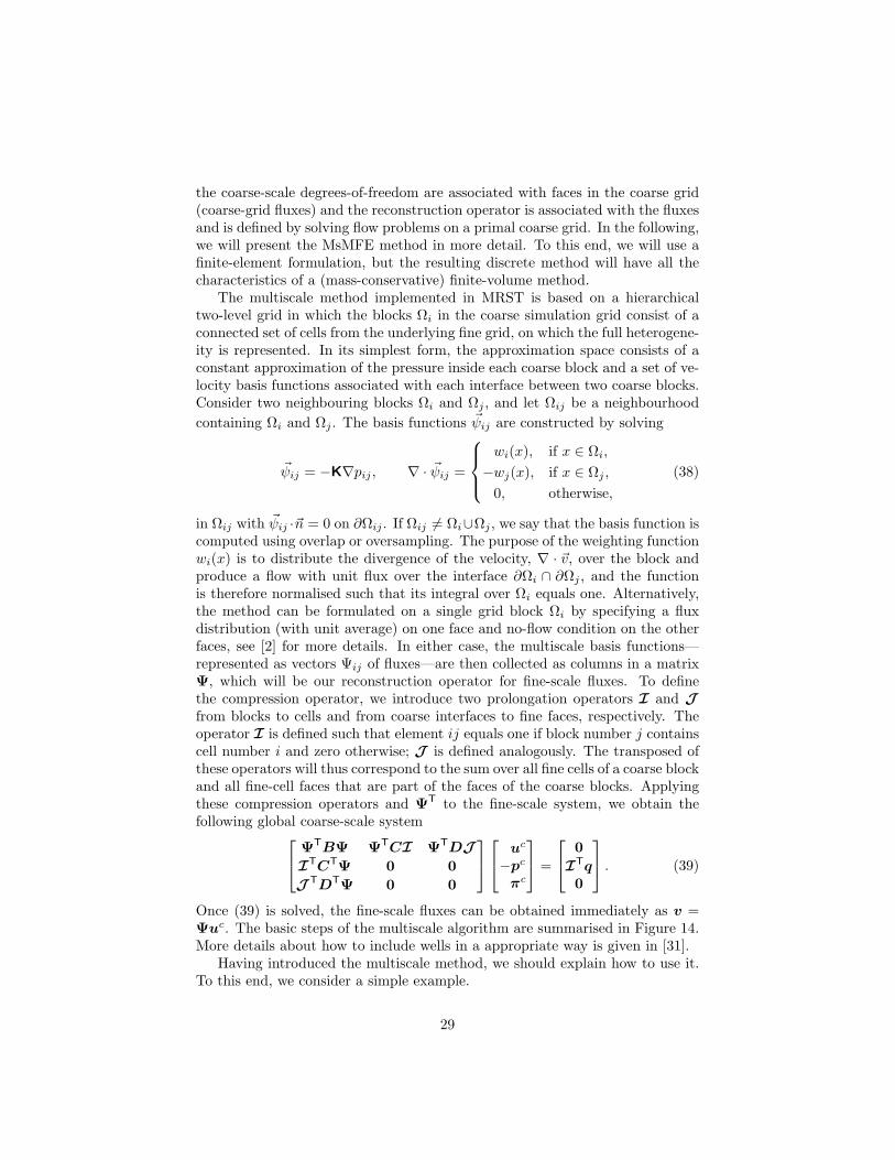
Once (39) is solved, the fine-scale fluxes can be obtained immediately as v =Ψuc. The basic steps of the multiscale algorithm are summarised in Figure 14.More details about how to include wells in a appropriate way is given in [31].
Having introduced the multiscale method, we should explain how to use it.To this end, we consider a simple example.
29
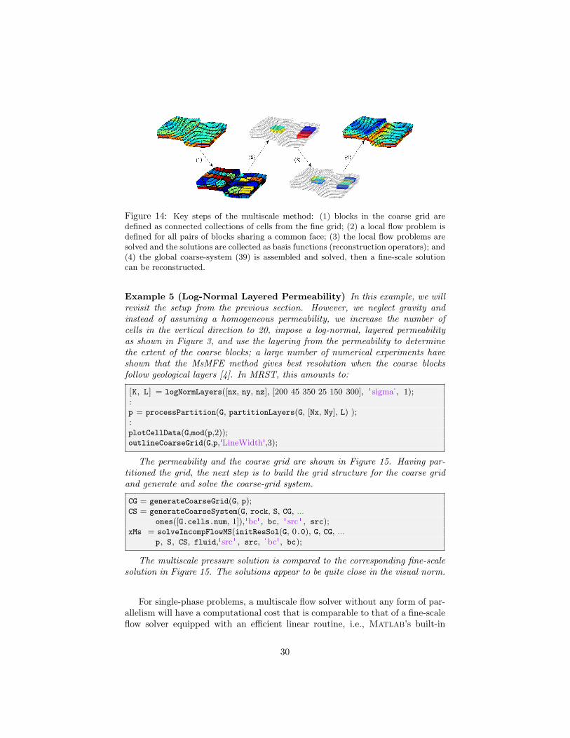
Figure 14: Key steps of the multiscale method: (1) blocks in the coarse grid aredefined as connected collections of cells from the fine grid; (2) a local flow problem isdefined for all pairs of blocks sharing a common face; (3) the local flow problems aresolved and the solutions are collected as basis functions (reconstruction operators); and(4) the global coarse-system (39) is assembled and solved, then a fine-scale solutioncan be reconstructed.
Example 5 (Log-Normal Layered Permeability) In this example, we willrevisit the setup from the previous section. However, we neglect gravity andinstead of assuming a homogeneous permeability, we increase the number ofcells in the vertical direction to 20, impose a log-normal, layered permeabilityas shown in Figure 3, and use the layering from the permeability to determinethe extent of the coarse blocks; a large number of numerical experiments haveshown that the MsMFE method gives best resolution when the coarse blocksfollow geological layers [4]. In MRST, this amounts to:
[K, L] = logNormLayers([nx, ny, nz], [200 45 350 25 150 300], 'sigma', 1);:p = processPartition(G, partitionLayers(G, [Nx, Ny], L) );:plotCellData(G,mod(p,2));outlineCoarseGrid(G,p,'LineWidth',3);
The permeability and the coarse grid are shown in Figure 15. Having par-titioned the grid, the next step is to build the grid structure for the coarse gridand generate and solve the coarse-grid system.
CG = generateCoarseGrid(G, p);CS = generateCoarseSystem(G, rock, S, CG, ...
ones([G.cells.num, 1]),'bc' , bc, ' src ' , src);xMs = solveIncompFlowMS(initResSol(G, 0.0), G, CG, ...
p, S, CS, fluid,'src ' , src, 'bc' , bc);
The multiscale pressure solution is compared to the corresponding fine-scalesolution in Figure 15. The solutions appear to be quite close in the visual norm.
For single-phase problems, a multiscale flow solver without any form of par-allelism will have a computational cost that is comparable to that of a fine-scaleflow solver equipped with an efficient linear routine, i.e., Matlab’s built-in
30
Permeability
50
100
150
200
250
300
350
400
450
Coarse partition
0
10
20
0
10
20
0
10
20
x
Fine−scale pressure
y 0
10
20
0
10
20
0
10
20
x
Multiscale pressure
y
10.1
10.2
10.3
10.4
10.5
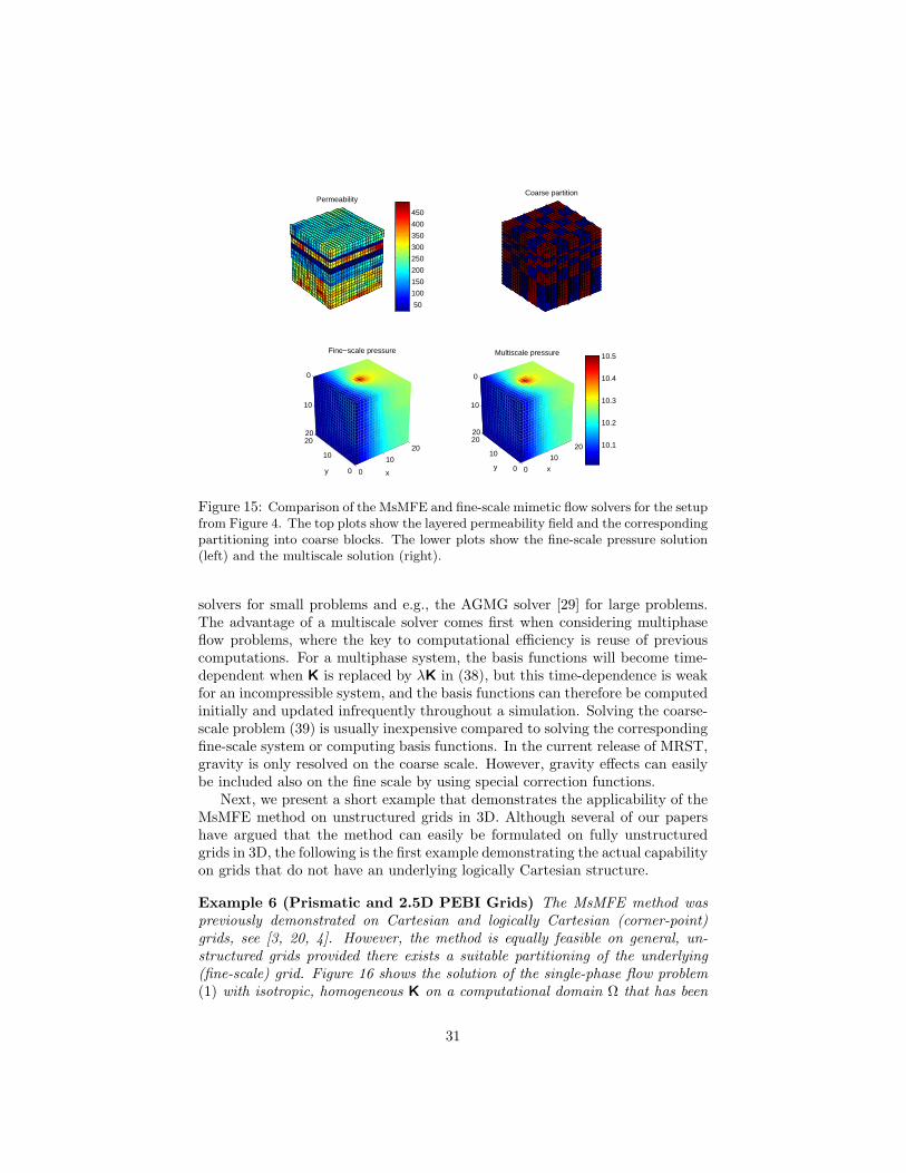
Figure 15: Comparison of the MsMFE and fine-scale mimetic flow solvers for the setupfrom Figure 4. The top plots show the layered permeability field and the correspondingpartitioning into coarse blocks. The lower plots show the fine-scale pressure solution(left) and the multiscale solution (right).
solvers for small problems and e.g., the AGMG solver [29] for large problems.The advantage of a multiscale solver comes first when considering multiphaseflow problems, where the key to computational efficiency is reuse of previouscomputations. For a multiphase system, the basis functions will become time-dependent when K is replaced by λK in (38), but this time-dependence is weakfor an incompressible system, and the basis functions can therefore be computedinitially and updated infrequently throughout a simulation. Solving the coarse-scale problem (39) is usually inexpensive compared to solving the correspondingfine-scale system or computing basis functions. In the current release of MRST,gravity is only resolved on the coarse scale. However, gravity effects can easilybe included also on the fine scale by using special correction functions.
Next, we present a short example that demonstrates the applicability of theMsMFE method on unstructured grids in 3D. Although several of our papershave argued that the method can easily be formulated on fully unstructuredgrids in 3D, the following is the first example demonstrating the actual capabilityon grids that do not have an underlying logically Cartesian structure.
Example 6 (Prismatic and 2.5D PEBI Grids) The MsMFE method waspreviously demonstrated on Cartesian and logically Cartesian (corner-point)grids, see [3, 20, 4]. However, the method is equally feasible on general, un-structured grids provided there exists a suitable partitioning of the underlying(fine-scale) grid. Figure 16 shows the solution of the single-phase flow problem(1) with isotropic, homogeneous K on a computational domain Ω that has been
31
Triangular coarse grid Multiscale pressure solution
PEBI coarse grid Multiscale pressure solution
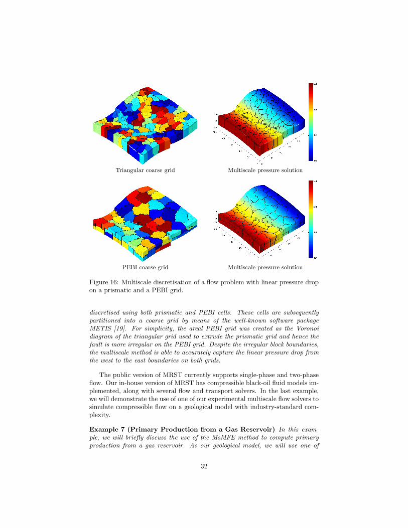
Figure 16: Multiscale discretisation of a flow problem with linear pressure dropon a prismatic and a PEBI grid.
discretised using both prismatic and PEBI cells. These cells are subsequentlypartitioned into a coarse grid by means of the well-known software packageMETIS [19]. For simplicity, the areal PEBI grid was created as the Voronoidiagram of the triangular grid used to extrude the prismatic grid and hence thefault is more irregular on the PEBI grid. Despite the irregular block boundaries,the multiscale method is able to accurately capture the linear pressure drop fromthe west to the east boundaries on both grids.
The public version of MRST currently supports single-phase and two-phaseflow. Our in-house version of MRST has compressible black-oil fluid models im-plemented, along with several flow and transport solvers. In the last example,we will demonstrate the use of one of our experimental multiscale flow solvers tosimulate compressible flow on a geological model with industry-standard com-plexity.
Example 7 (Primary Production from a Gas Reservoir) In this exam-ple, we will briefly discuss the use of the MsMFE method to compute primaryproduction from a gas reservoir. As our geological model, we will use one of
32
Permeability
Coarse grid
Rate in well perforation (m3/day)
100 200 400 600 800 1000535
540
545
550
555
560
Reference
5⋅10−2
5⋅10−4
5⋅10−6
5⋅10−7
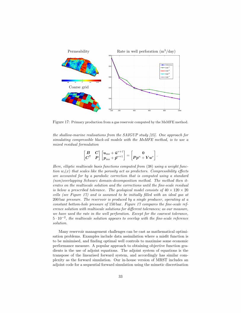
Figure 17: Primary production from a gas reservoir computed by the MsMFE method.
the shallow-marine realisations from the SAIGUP study [25]. One approach forsimulating compressible black-oil models with the MsMFE method, is to use amixed residual formulation[
B C
CT P
] [ums + uν+1
pms + pν+1
]=[
0Ppn + V uν
].
Here, elliptic multiscale basis functions computed from (38) using a weight func-tion wi(x) that scales like the porosity act as predictors. Compressibility effectsare accounted for by a parabolic correction that is computed using a standard(non)overlapping Schwarz domain-decomposition method. The method then it-erates on the multiscale solution and the corrections until the fine-scale residualis below a prescribed tolerance. The geological model consists of 40 × 120 × 20cells (see Figure 17) and is assumed to be initially filled with an ideal gas at200 bar pressure. The reservoir is produced by a single producer, operating at aconstant bottom-hole pressure of 150 bar. Figure 17 compares the fine-scale ref-erence solution with multiscale solutions for different tolerances; as our measure,we have used the rate in the well perforation. Except for the coarsest tolerance,5 · 10−2, the multiscale solution appears to overlap with the fine-scale referencesolution.
Many reservoir management challenges can be cast as mathematical optimi-sation problems. Examples include data assimilation where a misfit function isto be minimised, and finding optimal well controls to maximise some economicperformance measure. A popular approach to obtaining objective function gra-dients is the use of adjoint equations. The adjoint system of equations is thetranspose of the linearised forward system, and accordingly has similar com-plexity as the forward simulation. Our in-house version of MRST includes anadjoint code for a sequential forward simulation using the mimetic discretisation
33
for the pressure equation and an implicit version of the scheme (7) for satura-tion. In addition, an adjoint code for the multiscale method combined with theflow based coarsening approach is included, see [22].
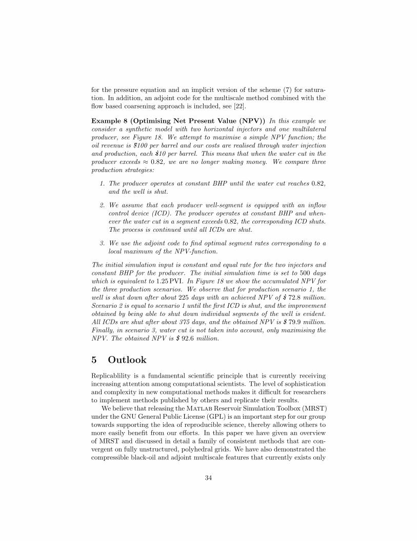
Example 8 (Optimising Net Present Value (NPV)) In this example weconsider a synthetic model with two horizontal injectors and one multilateralproducer, see Figure 18. We attempt to maximise a simple NPV function; theoil revenue is $100 per barrel and our costs are realised through water injectionand production, each $10 per barrel. This means that when the water cut in theproducer exceeds ≈ 0.82, we are no longer making money. We compare threeproduction strategies:
1. The producer operates at constant BHP until the water cut reaches 0.82,and the well is shut.
2. We assume that each producer well-segment is equipped with an inflowcontrol device (ICD). The producer operates at constant BHP and when-ever the water cut in a segment exceeds 0.82, the corresponding ICD shuts.The process is continued until all ICDs are shut.
3. We use the adjoint code to find optimal segment rates corresponding to alocal maximum of the NPV-function.
The initial simulation input is constant and equal rate for the two injectors andconstant BHP for the producer. The initial simulation time is set to 500 dayswhich is equivalent to 1.25 PVI. In Figure 18 we show the accumulated NPV forthe three production scenarios. We observe that for production scenario 1, thewell is shut down after about 225 days with an achieved NPV of $ 72.8 million.Scenario 2 is equal to scenario 1 until the first ICD is shut, and the improvementobtained by being able to shut down individual segments of the well is evident.All ICDs are shut after about 375 days, and the obtained NPV is $ 79.9 million.Finally, in scenario 3, water cut is not taken into account, only maximising theNPV. The obtained NPV is $ 92.6 million.
5 Outlook
Replicablility is a fundamental scientific principle that is currently receivingincreasing attention among computational scientists. The level of sophisticationand complexity in new computational methods makes it difficult for researchersto implement methods published by others and replicate their results.
We believe that releasing the Matlab Reservoir Simulation Toolbox (MRST)under the GNU General Public License (GPL) is an important step for our grouptowards supporting the idea of reproducible science, thereby allowing others tomore easily benefit from our efforts. In this paper we have given an overviewof MRST and discussed in detail a family of consistent methods that are con-vergent on fully unstructured, polyhedral grids. We have also demonstrated thecompressible black-oil and adjoint multiscale features that currently exists only
34
Permeability
Initial saturation and wells
Accumulated NPV
0 100 200 300 400 5000
2
4
6
8
10x 10
7
Time [days]
NP
V [$]
ReactiveReactive − ICDOptimal − ICD
Figure 18: Accumulated net present value for the three production strategies.
in our in-house, development version of the package. Although we are not yetthere, we are aiming towards a state where our publications on new computa-tional methodologies can be accompanied by open-access software that can beused by others to verify our computational results.
6 Acknowledgements
The research was funded in part by the Research Council of Norway throughgrants no. 158908, 174551, 175962, 178013, and 186935.
References
[1] Aarnes, J.E., Gimse, T., Lie, K.A.: An introduction to the numerics offlow in porous media using Matlab. In: G. Hasle, K.A. Lie, E. Quak (eds.)Geometrical Modeling, Numerical Simulation and Optimisation: IndustrialMathematics at SINTEF, pp. 265–306. Springer Verlag, Berling HeidelbergNew York (2007)
[2] Aarnes, J.E., Kippe, V., Lie, K.A.: Mixed multiscale finite elements andstreamline methods for reservoir simulation of large geomodels. Adv. WaterResour. 28(3), 257–271 (2005)
[3] Aarnes, J.E., Krogstad, S., Lie, K.A.: A hierarchical multiscale method fortwo-phase flow based upon mixed finite elements and nonuniform coarsegrids. Multiscale Model. Simul. 5(2), 337–363 (electronic) (2006)
35
[4] Aarnes, J.E., Krogstad, S., Lie, K.A.: Multiscale mixed/mimetic methodson corner-point grids. Comput. Geosci. 12(3), 297–315 (2008). DOI 10.1007/s10596-007-9072-8
[5] Aavatsmark, I.: An introduction to multipoint flux approximations forquadrilateral grids. Comput. Geosci. 6, 405–432 (2002). DOI 10.1023/A:1021291114475
[6] Aavatsmark, I., Barkve, T., Bøe, Ø., Mannseth, T.: Discretization on non-orthogonal, curvilinear grids for multi-phase flow. Proc. of the 4th Euro-pean Conf. on the Mathematics of Oil Recovery (1994)
[7] Aziz, K., Settari, A.: Petroleum Reservoir Simulation. Elsevier AppliedScience Publishers, London and New York (1979)
[8] Brezzi, F., Fortin, M.: Mixed and Hybrid Finite Element Methods,Springer Series in Computational Mathematics, vol. 15. Springer-Verlag,New York (1991)
[9] Brezzi, F., Lipnikov, K., Simoncini, V.: A family of mimetic finite differencemethods on polygonial and polyhedral meshes. Math. Models MethodsAppl. Sci. 15, 1533–1553 (2005). DOI 10.1142/S0218202505000832
[10] Chavent, G., Jaffre, J.: Mathematical models and finite elements for reser-voir simulation. North Holland (1982)
[11] Chen, Z., Hou, T.: A mixed multiscale finite element method for ellipticproblems with oscillating coefficients. Math. Comp. 72, 541–576 (2003)
[12] Deutsch, C.V., Journel, A.G.: GSLIB: Geostatistical software library anduser’s guide, 2nd edn. Oxford University Press, New York (1998)
[13] Durlofsky, L.J.: Upscaling and gridding of fine scale geological models forflow simulation (2005). Presented at 8th International Forum on ReservoirSimulation Iles Borromees, Stresa, Italy, June 20–24, 2005
[14] Edwards, M.G., Rogers, C.F.: A flux continuous scheme for the full tensorpressure equation. Proc. of the 4th European Conf. on the Mathematics ofOil Recovery (1994)
[15] Efendiev, Y., Hou, T.Y.: Multiscale Finite Element Methods, Surveys andTutorials in the Applied Mathematical Sciences, vol. 4. Springer Verlag(2009)
[16] Farmer, C.L.: Upscaling: a review. Int. J. Numer. Meth. Fluids 40(1–2),63–78 (2002). DOI 10.1002/fld.267
[17] Hou, T., Wu, X.H.: A multiscale finite element method for elliptic problemsin composite materials and porous media. J. Comput. Phys. 134, 169–189(1997)
36
[18] Jenny, P., Lee, S.H., Tchelepi, H.A.: Multi-scale finite-volume method forelliptic problems in subsurface flow simulation. J. Comput. Phys. 187,47–67 (2003)
[19] Karypis, G., Kumar, V.: A fast and high quality multilevel scheme forpartitioning irregular graphs. In: International Conference on Parallel Pro-cessing, pp. 113–122 (1995)
[20] Kippe, V., Aarnes, J.E., Lie, K.A.: A comparison of multiscale methodsfor elliptic problems in porous media flow. Comput. Geosci. 12(3), 377–398(2008). DOI 10.1007/s10596-007-9074-6
[21] Klausen, R.A., Stephansen, A.F.: Mimetic MPFA. In: Proc. 11th Euro-pean Conference on the Mathematics of Oil Recovery, 8-11 Sept., Bergen,Norway, A12. EAGE (2008)
[22] Krogstad, S., Hauge, V.L., Gulbransen, A.F.: Adjoint multiscale mixedfinite elements. SPE J. 16(1), 162–171 (2011). DOI 10.2118/119112-PA
[23] Ligaarden, I.S.: Well Models for Mimetic Finite Difference Methods andImproved Representation of Wells in Multiscale Methods. Master Thesis,University of Oslo (2008)
[24] Lipnikov, K., Shashkov, M., Yotov, I.: Local flux mimetic finite differ-ence methods. Numer. Math. 112(1), 115–152 (2009). DOI 10.1007/s00211-008-0203-5
[25] Manzocchi, T.., et al.: Sensitivity of the impact of geological uncertaintyon production from faulted and unfaulted shallow-marine oil reservoirs:objectives and methods. Petrol. Geosci. 14(1), 3–15 (2008)
[26] The MATLAB Reservoir Simulation Toolbox, version 2011a (2011). URLhttp://www.sintef.no/MRST/
[27] Muskat, M.: The flow of homogeneous fluid through porous media. McGrawHill Book Co., Inc, New York (1937)
[28] Natvig, J.R., Lie, K.A.: Fast computation of multiphase flow in porousmedia by implicit discontinuous Galerkin schemes with optimal ordering ofelements. J. Comput. Phys. 227(24), 10,108–10,124 (2008). DOI 10.1016/j.jcp.2008.08.024
[29] Notay, Y.: An aggregation-based algebraic multigrid method. ElectronicTransactions on Numerical Analysis 37, 123–146 (2010)
[30] Peaceman, D.W.: Interpretation of well-block pressures in numerical reser-voir simulation with nonsquare grid blocks and anisotropic permeability.SPE, Trans. AIME 275, 10–22 (1983)
37

[31] Skaflestad, B., Krogstad, S.: Multiscale/mimetic pressure solvers with near-well grid adaption. In: Proceedings of ECMOR XI–11th European Con-ference on the Mathematics of Oil Recovery, A36. EAGE, Bergen, Norway(2008)
[32] Zhou, H., Tchelepi, H.: Operator-based multiscale method for compressibleflow. SPE J. 13(2), 267–273 (2008)
38