paradygmaty ewolucji naukowo-kulturalnej w pracach ilyi...

Paradygmaty ewolucji naukowo-kulturalnej w pracach Ilyi Prigogine’a

1

Plus ratio quam vis

Ewa Gudowska-Nowak

Instytut Fizyki im. M. Smoluchowskiego i Centrum Badania Układów Złożonychim. M. Kaca, Uniwersytet Jagielloński w Krakowie

Studium Generale Universitatis Wratislaviensis, 28.02.2012

ZŁOŻONOŚĆ, PRZYPADEK,

SAMOORGANIZACJA:

wtorek, 13 marca 2012

2

lIya Prigogine 1917-2003Nagroda Nobla 1977

Tworzenie jest podstawową cechą Wszechświata, akreatywność naukowa równoległa do kreatywności artystycznej ...(z wywiadu z E.Lévy, Le Point, 18.01,2002)

„Nasza wizja przyrody ulega gruntownej zmianie ewoluując ku wielości, czasowości i złożoności...

Zasada wzrostu entropii opisuje świat jako uklad przechodzący stopniowo do chaosu. Tymczasem ewolucja systemów biologicznych czy społecznych dowodzi, że to, co złożone wyłania się z tego, co proste...

Brak równowagi , którego wyrazem jest przepływ materii i energii, może być źródłem porządku...”

I.Prigogine, I. Stengers „Z chaosu ku porządkowi: Nowy dialog człowieka z przyrodą”, PIW, 1990


3

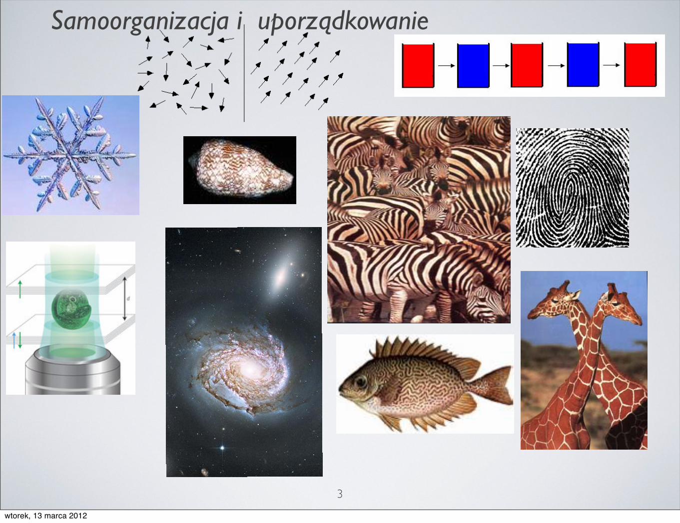
Samoorganizacja i uporządkowanie


4

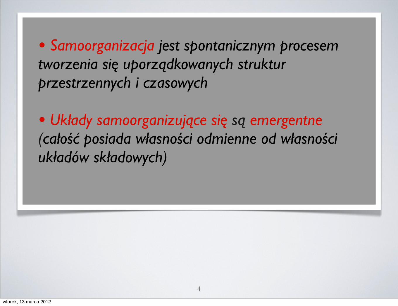
• Samoorganizacja jest spontanicznym procesem tworzenia się uporządkowanych struktur przestrzennych i czasowych

• Układy samoorganizujące się są emergentne(całość posiada własności odmienne od własności układów składowych)


5

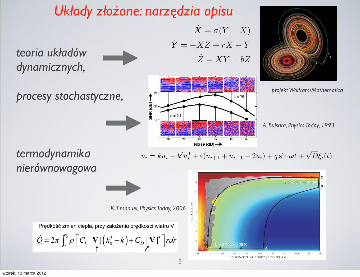
teoria układów dynamicznych,

procesy stochastyczne,

termodynamika nierównowagowa

X = σ(Y −X)

Y = −XZ + rX − Y

Z = XY − bZ

ui = kui − k�u3i + ε(ui+1 + ui−1 − 2ui) + q sinωt+

√Dξi(t)

tial evaporation rates, the air a short distance above the seasurface must be much drier than would be the case were it inequilibrium with the sea.

The figure illustrates the four legs of a hurricane Carnotcycle. From A to B, air undergoes nearly isothermal expan-sion as it flows toward the lower pressure of the storm cen-ter while in contact with the surface of the ocean, a giant heatreservoir. As air spirals in near the surface, conservation ofangular momentum causes the air to rotate faster about thestorm’s axis. Evaporation of seawater transfers energy fromthe sea to the air and increases the air’s entropy.

Once the air reaches the point where the surface wind isstrongest—typically 5–100 km from the center of the hurri-cane—it turns abruptly (point B in the figure) and flows up-ward within the sloping ring of cumulonimbus cloud knownas the eyewall. The ascent is nearly adiabatic. In real stormsthe air flows out at the top of its trajectory (point C in the fig-ure) and is incorporated into other weather systems; in ide-alized models one can close the cycle by allowing the heat ac-quired from the sea surface to be isothermally radiated tospace as IR radiation from the storm outflow. Finally, thecycle is completed as air undergoes adiabatic compressionfrom D to A.

The rate of heat transfer from the ocean to the atmos-phere varies as vE, where v is the surface wind speed and Equantifies the thermodynamic disequilibrium between theocean and atmosphere. But there is another source of heat;the dissipation of the kinetic energy of the wind by surfacefriction. That can be shown to vary as v3. According to Carnot,the power generation by the hurricane heat engine is givenby the rate of heat input multiplied by the thermodynamicefficiency:

If the storm is in a steady condition, then the power gen-eration must equal the dissipation, which is proportional tov3. Equating dissipation and generation yields an expressionfor the wind speed:

Here Ts is the ocean temperature and To is the temperatureof the outflow. Those temperatures and E may be easily esti-mated from observations of the tropics, and v as given by theabove equation is found to provide a good quantitative upperbound on hurricane wind speeds. Several factors, however,prevent most storms from achieving their maximum sus-tainable wind speed, or “potential intensity.” Those includecooling of the sea surface by turbulent mixing that bringscold ocean water up to the surface and entropy consumptionby dry air finding its way into the hurricane’s core.The thermodynamic cycle of a hurricane represents only aglimpse of the fascinating physics of hurricanes; more com-plete expositions are available in the resources given below.The transition of the tropical atmosphere from one with or-dinary convective clouds and mixing-dominated entropyproduction to a system with powerful vortices and dissipa-tion-driven entropy production remains a mysterious and in-adequately studied phenomenon. This may be of more thanacademic interest, as increasing concentrations of green-house gases increase the thermodynamic disequilibrium ofthe tropical ocean–atmosphere system and thereby increasethe intensity of hurricanes.

Additional resources! K. Emanuel, Annu. Rev. Earth Planet Sci. 31, 75 (2003).! K. Emanuel, Divine Wind: The History and Science of Hurri-canes, Oxford U. Press, New York (2005). !

www.physicstoday.org August 2006 Physics Today 3

The hurricane as aCarnot heat engine.This two-dimensionalplot of the thermody-namic cycle shows avertical cross section ofthe hurricane, whosestorm center lies alongthe left edge. Colorsdepict the entropy dis-tribution; cooler colorsindicate lower entropy.The process mainlyresponsible for drivingthe storm is the evapo-ration of seawater,which transfers energyfrom sea to air. As aresult of that transfer,air spirals inward fromA to B and acquiresentropy at a constanttemperature. It thenundergoes an adiabat-ic expansion from B toC as it ascends within

the storm’s eyewall. Far from the storm center, symbolicallybetween C and D, it exports IR radiation to space and soloses the entropy it acquired from the sea. The depicted com-pression is very nearly isothermal. Between D and A the airundergoes an adiabatic compression. Voilà, the four legs of aCarnot cycle.

The online version of this Quick Study provides links to images ofhurricanes.

projekt Wolfram/Mathematica

A. Bulsara, Physics Today, 1993

K. Emanuel, Physics Today, 2006

Układy złożone: narzędzia opisu


6

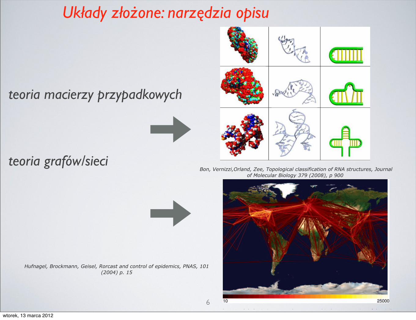
teoria macierzy przypadkowych

teoria grafów/sieciTable 1: Examples of basic RNA secondary structure motifs. From top to bottom: a single strand(PDB 283D [5]), a helical duplex (PDB 405d [6]), a hairpin stem and loop (PDB 1e4p [7]), a bulge(PDB 1r7w [8]), a multiloop (PDB 1kh6 [9]). From left to right: spacefill view, three-dimensionalstructure, secondary structure motif. The pictures are made with MolPov [10], Jmol [11] and PovRay[12].

3

Bon, Vernizzi,Orland, Zee, Topological classification of RNA structures, Journal of Molecular Biology 379 (2008), p 900

In addition to this dynamics, one must specify the initial condi-tion p(S, I; t ! t0), which is typically assumed to be a small butfixed number of infecteds I0, i.e., p(S, I; t ! t0) ! !I,I0!S,N"I0.

The relation of the probabilistic master equation 3 to thedeterministic SIR model (1) can be made in the limit of a large butfinite population, i.e., N ## 1. In this limit, one can approximate themaster equation by a Fokker–Planck equation by means of anexpansion in terms of conditional moments [Kramers–Moyal ex-pansion (13); see supporting information, which is published on thePNAS web site]. The associated description in terms of stochasticLangevin equations reads

ds!dt " "#sj $1

"N"#sj%1$ t% [4]

dj!dt " #sj & ' j &1

"N"#sj%1$ t% $

1"N

"' j%2$ t% .

[5]

Here, the independent Gaussian white noise forces %1(t) and %2(t)reflect the fluctuations of transmission and recovery, respectively.Note that the magnitude of the fluctuations are & 1!'N anddisappear in the limit N3 (, in which case Eqs. 1 are recovered.However, for large but finite N, a crucial difference is apparent:Eqs. 4 and 5 contain fluctuating forces, and N is a parameter of thesystem. A careful analysis shows that even for very large populations(i.e., N ## 1), fluctuations play a prominent role in the initial phaseof an epidemic outbreak and cannot be neglected. For instance,even when (0 # 0, a small initial number of infecteds in a populationmay not necessarily lead to an outbreak that cannot be accountedfor by the deterministic model.

Dispersal on the Aviation NetworkAs individuals travel around the world, the disease may spreadfrom one place to another. To quantify the traveling behavior of

individuals, we have analyzed all national and international civilf lights among the 500 largest airports by passenger capacity.‡This analysis yields the global aviation network shown in Fig. 1;further details of the data collection are compiled in thesupporting information. The strength of a connection betweentwo airports is given by passenger capacity, i.e., the number ofpassengers that travel a given route per day.

We incorporate the global dispersion of individuals into ourmodel by dividing the population into M local urban populationslabeled i containing Ni individuals. For each i, the number ofsusceptible and infected individuals is given by Si and Ii, respec-tively. In each urban area, the infection dynamics is governed bymaster equation 3.

Stochastic dispersal of individuals is defined by a matrix )ij oftransition probability rates among populations

SiO¡)ij

Sj IiO¡)ij

Ij, i, j " 1, . . . , M, [6]

where )ii ! 0. Along the same lines as presented above, one canformulate a master equation for the pair of vectors X ! {S1,I1, . . . , SM, IM}, which defines the stochastic state of the system.This master equation is provided explicitly in Eq. 3, supportinginformation.

To account for the global spread of an epidemic via theaviation network, one needs to specify the matrix )ij. Because the

‡Data on flight schedules and airport information are available from OAG WorldwideLimited, London (www.oag.com), and the International Air Transport Association, Geneva(www.iata.org).

Fig. 1. Global aviation network. A geographical representation of the civilaviation traffic among the 500 largest international airports in #100 differentcountries is shown. Each line represents a direct connection between airports.The color encodes the number of passengers per day (see color code at thebottom) traveling between two airports. The network accounts for #95% ofthe international civil aviation traffic. For each pair (i, j) of airports, we checkedall flights departing from airport j and arriving at airport i. The amount ofpassengers carried by a specific flight within 1 week can be estimated by thesize of the aircraft (We used manufacturer capacity information on #150different aircraft types) times the number of days the flight operates in 1week. The sum of all flights yields the passengers per week, i.e., Mij in Eq. 7. Wecomputed the total passenger capacity ) Mij of each airport j per week andfound very good agreement with independently obtained airport capacities.

Fig. 2. Global spread of SARS. (A) Geographical representation of the globalspreading of probable SARS cases on May 30, 2003, as reported by the WHOand Centers for Disease Control and Prevention. The first cases of SARSemerged in mid-November 2002 in Guangdong Province, China (17). Thedisease was then carried to Hong Kong on the February 21, 2003, and beganspreading around the world along international air travel routes, becausetourists and the medical doctors who treated the early cases traveled inter-nationally. As the disease moved out of southern China, the first hot zones ofSARS were Hong Kong, Singapore, Hanoi (Vietnam), and Toronto (Canada),but soon cases in Taiwan, Thailand, the U.S., Europe, and elsewhere werereported. (B) Geographical representation of the results of our simulations 90days after an initial infection in Hong Kong, The simulation corresponds to thereal SARS infection at the end of May 2003. Because our simulations cannotdescribe the infection in China, where the disease started in November 2002,we used the WHO data for China.

Hufnagel et al. PNAS # October 19, 2004 # vol. 101 # no. 42 # 15125

ECO

LOG

Y

Hufnagel, Brockmann, Geisel, Rorcast and control of epidemics, PNAS, 101 (2004) p. 15

Układy złożone: narzędzia opisu


7

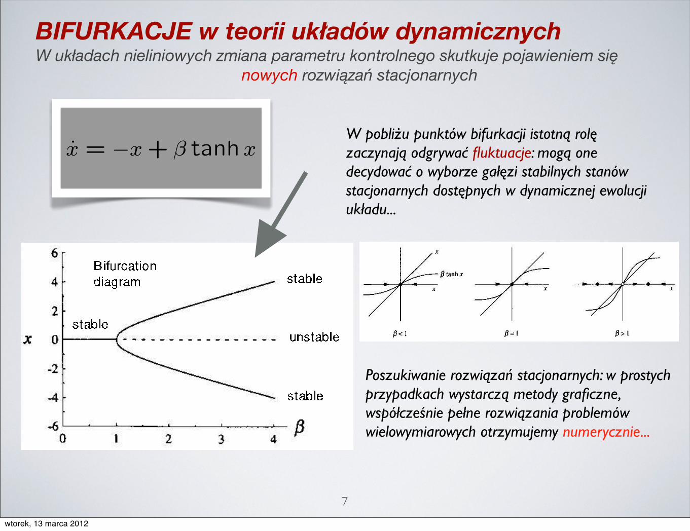
BIFURKACJE w teorii układów dynamicznychW układach nieliniowych zmiana parametru kontrolnego skutkuje pojawieniem się

nowych rozwiązań stacjonarnych

Example 3.4.1 x = !x + ! tanhx

Arises in statistical mechanical models e.g.of magnets or neural networks

Plot y = x and y = ! tanhx

Fig. 3.4.3

Fig. 3.4.413




Fig. 3.4.3

Fig. 3.4.413

W pobliżu punktów bifurkacji istotną rolę zaczynają odgrywać fluktuacje: mogą one decydować o wyborze gałęzi stabilnych stanów stacjonarnych dostępnych w dynamicznej ewolucjiukładu...




Fig. 3.4.3

Fig. 3.4.413

Poszukiwanie rozwiązań stacjonarnych: w prostych przypadkach wystarczą metody graficzne, współcześnie pełne rozwiązania problemów wielowymiarowych otrzymujemy numerycznie...


8

!"#"$%&'(%)*+,* %-''.% /0

1% 1,*23*% 45678*9% +*:1*8;9,%1+<=+2:,;>% ?*7:;9,% *3*@*827?8=;>% +: 7679 ;=;>% +, %87% ;7 =% 4?5;*+(% <5+27 % <74?54585178=% 654,*?5% 1% 3727;>% +,*6*@6<,*+, 2=;>A%B%?5:C% /&0-% !,*36(% DE?5+% ,% $5=*+(% 4?7;C9 ;=% 87% F8,1*?+=2*;,*% G278C% "?*H58(%<74?54585173,%+;>*@72%@*;>78,<@C%?*7:;9,%+: 7679 ;=;>%+, %<%5+,*@87+2C%*274I1%J/KA% G=@C37;97% :5@4C2*?517% 4?<*4?5176<587% 617% 3727% 4I 8,*9% 651,56 7% 4?71L6<,15 ;,%2*H5%+;>*@72CA%%%

GMNOPQ#%ROQDM)S%TSO "FG"BQL QT"#U GDSOV"%%GCW+2?727@,% + % 2?<=% <1, <:,% 8,*5?H78,;<8*X% 958=% W?5@,7851*% % 958=%K(YJT?"W?5@:51*%JT?ZK%,%958=%;*?71*%JM*Y[K%5?7<%:17+%@735851=%JMN-JM""NK-KA%%%%/A%%%-N[%[%T?Z%[% %% %%N"T?%[%NT?"YT?" -%

%%-A%%%N[%[%NT?"-%[%T?Z%% %%-N"T?%%%YA%%%MN-JM""NK-%% %%J"NK-%M%\%MNM""N%%%]A%%%N"T?%[%T?Z%[%N[%% %%T?-%[%N-"%%%.A%%%TR-%[%J"NK-%M%\%MNM""N%% %%N[%[%T?Z%[%T?MNJM""NK-%%%^A%%%NT?"-%[% %[%NYT?" [%% %%-T?"-%[%N-"%

%%0A%%%T?"-%[%M*Y[%[N[%% %%M*][%[%NT?"-%%%_A%%%M*][%[%T?"-%[%N-"%% %% %[%-NYT?" [%[%M*Y[%

%%&A%%%-NT?"-%% %%N"T?%[% %[%NYT?" [%

/'A%%%M*][%[%MN-JM""NK-%% %%MNJM""NK-%[%M*Y[%[%N[%//A%%%MNJM""NK-%[%T?MNJM""NK-%[%N-"%% %%T?Z%[%MN-JM""NK-%[%%%%%%%%%%%%%%%%%%%%%%%%%%%%%%%%%%%%%%%%%%%%%%%%%%%%%%%%%%%%%%%%%%%%%%%%%%%%%%%%%%%%%%%%%%%%%%[%N"MJM""NK-%[%N[%/-A%%%M*][%[%T?MNJM""NK-%[%N-"% %%T?Z%[%N"MJM""NK-%[%M*Y[%[%-N[%/YA%%%-N"MJM""NK-%% %%N"MNJM""NK-%[%M%\%MNM"""N%[%M"-%/]A%%%M*][%[%N"MNJM""NK-%% %%N"MJM""NK-%[%M*Y[%[%N[%/.A%%%M*][%[%"%\%MNM""N%% %%"%\%MM""N%[%M*Y[%[%N[%/^A%%%-%"%\%MM""N%[%N-"%% %%"%\%MNM""N%[%NM""N%[%M"-%/0A%%%T?-%[%NM""N%% %%-T?Z%[%M"-%[%-N[%/_A%%%-%MNJM""NK-%[%N-"% %MN-JM""NK-%[%N"MNJM""NK-%%`?56C:27@,%:5 ;51=@,%+ X%61C23*8*:%1 H37(%:17+%@?I1:51=%JNM""NK%,%:17+%W?5@5@735851=% JT?MNJM""NK-KA% T7?17% ?5<215?C% 5+;=3C9*% 45@, 6<=% I 2 %J;*?%87%;<17?2=@%+2548,C%C23*8,*8,7K%,%4?<*9?<=+2 %J;*?%87%2?<*;,@%+2548,C%C23*L8,*8,7KA%

%

F. Sagues, I. Epstein Dalton Trans. 1201, (2003)

Cykliczna zmiana stężeń reagentów w czasie: przykład

zegara chemicznego

Reakcja Biełousowa-Żabotyńskiego


9

L!! B"1#!2 A2

"B "A2#D!2" . "3#

Perturbations u are expanded in normal modes u!$ #k#!kc

u0 exp%&(k)t#ik•r' leading to the eigenvalue equa-tion &(k)2"(&(k)#)!0 in which ( and ) indicate thetrace and the determinant of the linear operator L, respec-tively. Depending on the values of the parameters A and Dthe system will undergo a Turing "stationary# bifurcation or aHopf instability. As a matter of fact, 2D reaction-diffusionsystems that display Turing patterns also present a Hopf bi-furcation. The latter gives rise to oscillations if *+!1/D$(!1#A2"1)/A %14'. Otherwise, a Turing instability takesplace, the case we focus on hereafter.The marginal condition (&!0) leads to a curve B

!B(k) the minimum of which yields the critical point(Bc ,kc)!%(1#A*)2,!A*' . To describe naturally the sepa-ration from the critical values the rescaled parameter ,!(B"Bc)/Bc dubbed supercriticality, replaces B as the con-trol parameter.Before going to a perturbative analysis let us show ex-

amples of Turing patterns from direct simulations of themodel in Fig. 1, similar to that obtained by other authors%8,9'. They correspond to hexagons with different phases andstripes, for different values of the supercriticality , . Thesepatterns are shown here just as a guide to the ensuing weaklynonlinear analysis. "Technical details on the simulations willbe given in Sec. V C.#

III. WEAKLY NONLINEAR THEORY

Amplitude equations are a classical tool to describe ex-cited states beyond linear analysis %15'. We sketch briefly themain steps in obtaining them. Just above threshold the eigen-values of the critical modes are close to zero, so that they areslowly varying modes, whereas the off-critical modes relaxquickly, so only perturbations with k around kc have to beconsidered. The solution of Eq. "2# can be expanded as

u!$j!1

N

u0"A jeikj•r#c.c.#, "4#

where u0!„1,"*(1#A*)/A…T stands for the eigenvector ofthe linear operator. Here we use the standard multiple-scaleanalysis %15' in which the control parameter and the deriva-tives are expanded in terms of a small parameter - and or-

thogonality conditions "Fredholm alternative# are used ateach order. In the neighborhood of the bifurcation point, thecritical amplitudes A j follow the so-called normal forms.Their general form can be derived from standard techniquesof symmetry-breaking bifurcations %16'. A normal form de-scribes perfect extended patterns, but slight variations in thepattern can be included by means of spatial terms with thesuitable symmetries, so one arrives at the so-called amplitudeequations. We discuss in the following the form of theseequations for different planforms.Stripes are characterized by a single amplitude A that

evolves according to

(0. tA!,A"g#A#2A#/02! .x#

12ikc

.y2" 2A , "5#

which is the normal form for a supercritical bifurcation plusa term that accounts for spatial variations, known as theNewell–Whitehead–Segel equation %17' in convection phe-nomena.Squares are formed by two perpendicular sets of rolls

with equal wave numbers, i.e., "a# k1!k2 and "b# #k1#!#k2#.They display four peaks with D4 symmetry in Fourier space.When condition "b# does not hold one obtains rectangular orbimodal patterns; instead, without the condition "a# rhombs"rhombic cells# arise. Squares or rhombs should obeycoupled equations of the kind: (0. tA1!,A1"g#A1#2A1"g0#A2#A1, in which g0 depends on k1•k2 "valid for anglesnot around 21/3).Hexagons are built up by three modes satisfying the reso-

nant condition k1#k2#k3!0 "resonant triad#, with #k1#!#k2#!#k3#. When the modes break the rotational symmetrybut not reflexions (#k1#2#k2#!#k3#) squeezed hexagons re-sult. Distortions breaking rotation and reflexion symmetries,#k1#2#k2#2#k3#, lead to a pattern of sheared hexagons. Letus stress that what have been called ‘‘rhombs’’ or ‘‘rhombiccells’’ in many recent papers are actually distorted hexagons,a distinction far from semantic, because the term ‘‘rhomb’’used for a three-mode pattern has induced some misleadinginterpretations %18'. Squares or true rhombs have never beenobserved in experiments, while slightly distorted hexagonshave been reported in chemical systems %6' and in theoreticalmodels %11,19'.During the last years several authors have established

that, up to the third order in the amplitudes, the general formof the amplitude equations for a hexagonal pattern should beas follows %11,12':

(0. tA1!,A1#/02.x12 A1#vA2A3"g#A1#2A1

"h" #A2#2##A3#2#A1#i31% A2.x3A3#A3.x2A2'

#i32% A2.(3A3"A3.(2

A2' , "6#

where subindices in the derivatives stand for .xi!ni•“ and.( i

! !i•“ , respectively, being ni the unitary vectors in thedirection of ki and !i orthogonal to ni . Companion equationsfor A2 and A3 are simply obtained by subindex permutations.

FIG. 1. Turing patterns from direct simulations of Brusselatormodel (A!4.5,D!8): "a# ,!0.04 initial hexagons, "b# ,!0.30striped pattern, and "c# ,!0.98 reentrant hexagons.

B. PENA AND C. PEREZ-GARCIA PHYSICAL REVIEW E 64 056213

056213-2

L!! B"1#!2 A2

"B "A2#D!2" . "3#

Perturbations u are expanded in normal modes u!$ #k#!kc

u0 exp%&(k)t#ik•r' leading to the eigenvalue equa-tion &(k)2"(&(k)#)!0 in which ( and ) indicate thetrace and the determinant of the linear operator L, respec-tively. Depending on the values of the parameters A and Dthe system will undergo a Turing "stationary# bifurcation or aHopf instability. As a matter of fact, 2D reaction-diffusionsystems that display Turing patterns also present a Hopf bi-furcation. The latter gives rise to oscillations if *+!1/D$(!1#A2"1)/A %14'. Otherwise, a Turing instability takesplace, the case we focus on hereafter.The marginal condition (&!0) leads to a curve B

!B(k) the minimum of which yields the critical point(Bc ,kc)!%(1#A*)2,!A*' . To describe naturally the sepa-ration from the critical values the rescaled parameter ,!(B"Bc)/Bc dubbed supercriticality, replaces B as the con-trol parameter.Before going to a perturbative analysis let us show ex-

amples of Turing patterns from direct simulations of themodel in Fig. 1, similar to that obtained by other authors%8,9'. They correspond to hexagons with different phases andstripes, for different values of the supercriticality , . Thesepatterns are shown here just as a guide to the ensuing weaklynonlinear analysis. "Technical details on the simulations willbe given in Sec. V C.#

III. WEAKLY NONLINEAR THEORY

Amplitude equations are a classical tool to describe ex-cited states beyond linear analysis %15'. We sketch briefly themain steps in obtaining them. Just above threshold the eigen-values of the critical modes are close to zero, so that they areslowly varying modes, whereas the off-critical modes relaxquickly, so only perturbations with k around kc have to beconsidered. The solution of Eq. "2# can be expanded as

u!$j!1

N

u0"A jeikj•r#c.c.#, "4#

where u0!„1,"*(1#A*)/A…T stands for the eigenvector ofthe linear operator. Here we use the standard multiple-scaleanalysis %15' in which the control parameter and the deriva-tives are expanded in terms of a small parameter - and or-

thogonality conditions "Fredholm alternative# are used ateach order. In the neighborhood of the bifurcation point, thecritical amplitudes A j follow the so-called normal forms.Their general form can be derived from standard techniquesof symmetry-breaking bifurcations %16'. A normal form de-scribes perfect extended patterns, but slight variations in thepattern can be included by means of spatial terms with thesuitable symmetries, so one arrives at the so-called amplitudeequations. We discuss in the following the form of theseequations for different planforms.Stripes are characterized by a single amplitude A that

evolves according to

(0. tA!,A"g#A#2A#/02! .x#

12ikc

.y2" 2A , "5#

which is the normal form for a supercritical bifurcation plusa term that accounts for spatial variations, known as theNewell–Whitehead–Segel equation %17' in convection phe-nomena.Squares are formed by two perpendicular sets of rolls

with equal wave numbers, i.e., "a# k1!k2 and "b# #k1#!#k2#.They display four peaks with D4 symmetry in Fourier space.When condition "b# does not hold one obtains rectangular orbimodal patterns; instead, without the condition "a# rhombs"rhombic cells# arise. Squares or rhombs should obeycoupled equations of the kind: (0. tA1!,A1"g#A1#2A1"g0#A2#A1, in which g0 depends on k1•k2 "valid for anglesnot around 21/3).Hexagons are built up by three modes satisfying the reso-

nant condition k1#k2#k3!0 "resonant triad#, with #k1#!#k2#!#k3#. When the modes break the rotational symmetrybut not reflexions (#k1#2#k2#!#k3#) squeezed hexagons re-sult. Distortions breaking rotation and reflexion symmetries,#k1#2#k2#2#k3#, lead to a pattern of sheared hexagons. Letus stress that what have been called ‘‘rhombs’’ or ‘‘rhombiccells’’ in many recent papers are actually distorted hexagons,a distinction far from semantic, because the term ‘‘rhomb’’used for a three-mode pattern has induced some misleadinginterpretations %18'. Squares or true rhombs have never beenobserved in experiments, while slightly distorted hexagonshave been reported in chemical systems %6' and in theoreticalmodels %11,19'.During the last years several authors have established

that, up to the third order in the amplitudes, the general formof the amplitude equations for a hexagonal pattern should beas follows %11,12':

(0. tA1!,A1#/02.x12 A1#vA2A3"g#A1#2A1

"h" #A2#2##A3#2#A1#i31% A2.x3A3#A3.x2A2'

#i32% A2.(3A3"A3.(2

A2' , "6#

where subindices in the derivatives stand for .xi!ni•“ and.( i

! !i•“ , respectively, being ni the unitary vectors in thedirection of ki and !i orthogonal to ni . Companion equationsfor A2 and A3 are simply obtained by subindex permutations.

FIG. 1. Turing patterns from direct simulations of Brusselatormodel (A!4.5,D!8): "a# ,!0.04 initial hexagons, "b# ,!0.30striped pattern, and "c# ,!0.98 reentrant hexagons.

B. PENA AND C. PEREZ-GARCIA PHYSICAL REVIEW E 64 056213

056213-2

Stability of Turing patterns in the Brusselator model

B. Pena and C. Perez-GarcıaInstituto de Fısica, Universidad de Navarra, E-31080 Pamplona, Spain

!Received 21 December 2000; revised manuscript received 18 June 2001; published 22 October 2001"

The selection and competition of Turing patterns in the Brusselator model are reviewed. The stability ofstripes and hexagons towards spatial perturbations is studied using the amplitude equation formalism. Forhexagonal patterns these equations include both linear and nonpotential spatial terms enabling distorted solu-tions. The latter modify substantially the stability diagrams and select patterns with wave numbers quitedifferent from the critical value. The analytical results from the amplitude formalism agree with direct simu-lations of the model. Moreover, we show that slightly squeezed hexagons are locally stable in a full range ofdistortion angles. The stability regions resulting from the phase equation are similar to those obtained numeri-cally by other authors and to those observed in experiments.

DOI: 10.1103/PhysRevE.64.056213 PACS number!s": 05.45.!a, 82.40.Bj, 82.40.Ck

I. INTRODUCTION

Some chemical systems out of equilibrium undergo a spa-tial symmetry breaking, leading to stationary pattern forma-tion on macroscopic scales #1$. The new stationary statesform periodic concentration structures with a wavelength in-dependent of the reactor geometry, the so-called Turing pat-terns #1$. Experimental evidence for Turing patterns was firstobtained in 1990 by Castets et al. #2$, in the well-knownchlorite–iodine–malonic acid !CIMA" reaction, and later onin the chlorine–dioxide iodine–malonic acid !CDIMA" reac-tion #3,4$, and in the polyacrilamide-methylene blue-oxygenreaction, althought in the latter the leading mechanism is stillunder discussion #5$. Depending on the control parameters!concentrations of reactants and diffusion coefficients", thedynamics of the CIMA or CDIMA reaction exhibits severalkinds of steady patterns close to onset: stripes, hexagons, and‘‘rhombs’’ #6$. !Usually, the so-called ‘‘black eyes’’ seem toarise from secondary bifurcations." Realistic reactiveschemes are, in general, quite complicated. Consequentlythey are replaced by simplified schemes, as the Brusselatormodel #7$, reproducing the observed patterns while dealingwith simple calculations #8–10$.In the present paper we will focus on stationary Turing

patterns arising in the Brusselator. We discuss and obtain ageneralized amplitude equation, including spatial modula-tions, for the planforms appearing in the model. This equa-tion has been obtained in many chemical models for stripepatterns only, but the hexagonal case has not been discussedin detail so far #8–10$. From symmetry arguments, someauthors established that it must include some nonpotentialquadratic terms besides the usual diffusive linear one#11,12$. By means of a multiple-scale technique we computethe coefficients of the amplitude equation for the Brusselator.Stationary solutions of this equation are stripes, hexagonswith two different phases, mixed modes, and distorted hexa-gons. A linear stability analysis sets the stability of thesestationary solutions in regard to amplitude disturbances.Another stability limit is obtained from phase perturba-

tions. In fact, amplitude varies much more rapidly in timethan phase does and, therefore, it becomes enslaved by theslowly varying phases. The slow dynamics of slight spatial

heterogeneities in the pattern can be described with a phaseequation for each stationary solution. The stability regionscomputed for the Brusselator can be considered as reminis-cent of the Busse’s balloon in thermal convection #13$.The paper is organized as follows. In Sec. II we introduce

the two-dimensional !2D" model and we give a general sur-vey of the linear analysis. In Sec. III we carry out a weaklynonlinear analysis using the multiple-scale method to derivethe amplitude equations. The stability of patterns towardshomogeneous perturbations !amplitude instabilities" is dis-cussed in Sec. IV. The stability regions for roll, perfect hexa-gons, and squeezed hexagons are explicitly computed. Wederive the linear phase equations for different kind of hexa-gons in Sec. V and we compare the stability diagrams ob-tained analytically with direct numerical simulations of theBrusselator model. Sec. VI summarizes our conclusions.

II. THE REACTION-DIFFUSION MODEL

The Brusselator is considered one of the simplestreaction-diffusion models exhibiting Turing and Hopf insta-bilities. The spatiotemporal evolution of the main variables isgiven by the following partial differential equations:

% tX"A!!B#1 "X#X2Y#&2X ,!1"

% tY"BX!X2Y#D&2Y ,

where X and Y denote the concentrations of activator andsubstrate, respectively. Here D is a parameter proportional tothe diffusion ratio of the two species DY /DX and, as usual, Bis kept as the control parameter of the problem.The homogeneous steady state of these equations is sim-

ply us"(Xs ,Y s)"(A ,B/A) #9$. Let us briefly recall here theresults of the linear stability analysis around us . Consideringsmall perturbations u"(x ,y) in Eqs. !1" one arrives at

% tu"Lu#! BA x2#2Axy#x2y " ! 1!1 " , !2"

where L is the linearized operator

PHYSICAL REVIEW E, VOLUME 64, 056213

1063-651X/2001/64!5"/056213!9"/$20.00 ©2001 The American Physical Society64 056213-1

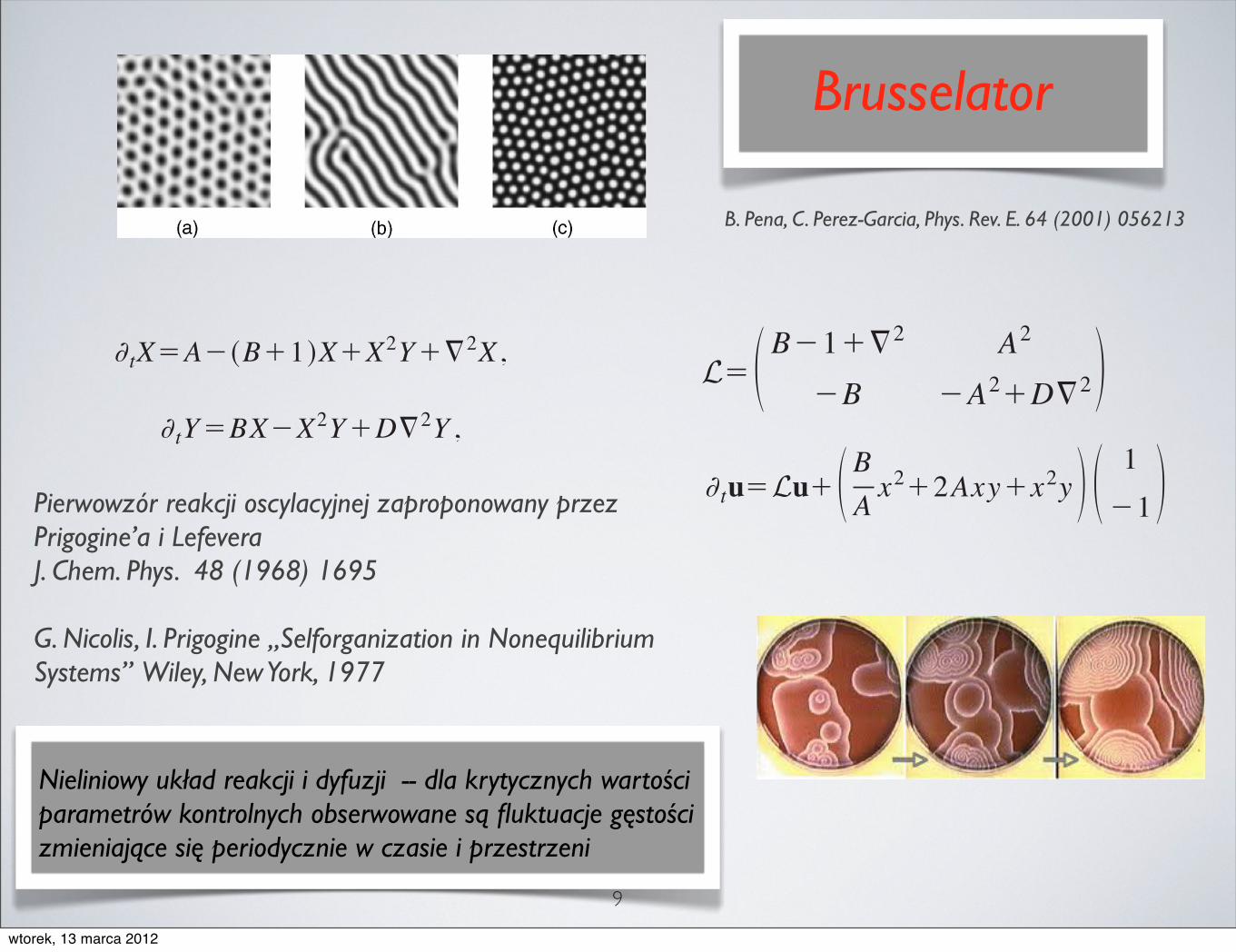
Pierwowzór reakcji oscylacyjnej zaproponowany przez Prigogine’a i LefeveraJ. Chem. Phys. 48 (1968) 1695

G. Nicolis, I. Prigogine „Selforganization in Nonequilibrium Systems” Wiley, New York, 1977

B. Pena, C. Perez-Garcia, Phys. Rev. E. 64 (2001) 056213

Brusselator

Stability of Turing patterns in the Brusselator model

B. Pena and C. Perez-GarcıaInstituto de Fısica, Universidad de Navarra, E-31080 Pamplona, Spain

!Received 21 December 2000; revised manuscript received 18 June 2001; published 22 October 2001"

The selection and competition of Turing patterns in the Brusselator model are reviewed. The stability ofstripes and hexagons towards spatial perturbations is studied using the amplitude equation formalism. Forhexagonal patterns these equations include both linear and nonpotential spatial terms enabling distorted solu-tions. The latter modify substantially the stability diagrams and select patterns with wave numbers quitedifferent from the critical value. The analytical results from the amplitude formalism agree with direct simu-lations of the model. Moreover, we show that slightly squeezed hexagons are locally stable in a full range ofdistortion angles. The stability regions resulting from the phase equation are similar to those obtained numeri-cally by other authors and to those observed in experiments.

DOI: 10.1103/PhysRevE.64.056213 PACS number!s": 05.45.!a, 82.40.Bj, 82.40.Ck

I. INTRODUCTION

Some chemical systems out of equilibrium undergo a spa-tial symmetry breaking, leading to stationary pattern forma-tion on macroscopic scales #1$. The new stationary statesform periodic concentration structures with a wavelength in-dependent of the reactor geometry, the so-called Turing pat-terns #1$. Experimental evidence for Turing patterns was firstobtained in 1990 by Castets et al. #2$, in the well-knownchlorite–iodine–malonic acid !CIMA" reaction, and later onin the chlorine–dioxide iodine–malonic acid !CDIMA" reac-tion #3,4$, and in the polyacrilamide-methylene blue-oxygenreaction, althought in the latter the leading mechanism is stillunder discussion #5$. Depending on the control parameters!concentrations of reactants and diffusion coefficients", thedynamics of the CIMA or CDIMA reaction exhibits severalkinds of steady patterns close to onset: stripes, hexagons, and‘‘rhombs’’ #6$. !Usually, the so-called ‘‘black eyes’’ seem toarise from secondary bifurcations." Realistic reactiveschemes are, in general, quite complicated. Consequentlythey are replaced by simplified schemes, as the Brusselatormodel #7$, reproducing the observed patterns while dealingwith simple calculations #8–10$.In the present paper we will focus on stationary Turing

patterns arising in the Brusselator. We discuss and obtain ageneralized amplitude equation, including spatial modula-tions, for the planforms appearing in the model. This equa-tion has been obtained in many chemical models for stripepatterns only, but the hexagonal case has not been discussedin detail so far #8–10$. From symmetry arguments, someauthors established that it must include some nonpotentialquadratic terms besides the usual diffusive linear one#11,12$. By means of a multiple-scale technique we computethe coefficients of the amplitude equation for the Brusselator.Stationary solutions of this equation are stripes, hexagonswith two different phases, mixed modes, and distorted hexa-gons. A linear stability analysis sets the stability of thesestationary solutions in regard to amplitude disturbances.Another stability limit is obtained from phase perturba-

tions. In fact, amplitude varies much more rapidly in timethan phase does and, therefore, it becomes enslaved by theslowly varying phases. The slow dynamics of slight spatial

heterogeneities in the pattern can be described with a phaseequation for each stationary solution. The stability regionscomputed for the Brusselator can be considered as reminis-cent of the Busse’s balloon in thermal convection #13$.The paper is organized as follows. In Sec. II we introduce

the two-dimensional !2D" model and we give a general sur-vey of the linear analysis. In Sec. III we carry out a weaklynonlinear analysis using the multiple-scale method to derivethe amplitude equations. The stability of patterns towardshomogeneous perturbations !amplitude instabilities" is dis-cussed in Sec. IV. The stability regions for roll, perfect hexa-gons, and squeezed hexagons are explicitly computed. Wederive the linear phase equations for different kind of hexa-gons in Sec. V and we compare the stability diagrams ob-tained analytically with direct numerical simulations of theBrusselator model. Sec. VI summarizes our conclusions.

II. THE REACTION-DIFFUSION MODEL

The Brusselator is considered one of the simplestreaction-diffusion models exhibiting Turing and Hopf insta-bilities. The spatiotemporal evolution of the main variables isgiven by the following partial differential equations:

% tX"A!!B#1 "X#X2Y#&2X ,!1"

% tY"BX!X2Y#D&2Y ,

where X and Y denote the concentrations of activator andsubstrate, respectively. Here D is a parameter proportional tothe diffusion ratio of the two species DY /DX and, as usual, Bis kept as the control parameter of the problem.The homogeneous steady state of these equations is sim-

ply us"(Xs ,Y s)"(A ,B/A) #9$. Let us briefly recall here theresults of the linear stability analysis around us . Consideringsmall perturbations u"(x ,y) in Eqs. !1" one arrives at

% tu"Lu#! BA x2#2Axy#x2y " ! 1!1 " , !2"

where L is the linearized operator

PHYSICAL REVIEW E, VOLUME 64, 056213

1063-651X/2001/64!5"/056213!9"/$20.00 ©2001 The American Physical Society64 056213-1

Nieliniowy układ reakcji i dyfuzji -- dla krytycznych wartości parametrów kontrolnych obserwowane są fluktuacje gęstości zmieniające się periodycznie w czasie i przestrzeni


10

w w w.Sc iAm.com SC IENTIF IC AMERIC AN 67

DAN

IELA

NAO

MI M

OLN

AR

chines is very deep. Fluctuations of the chemical energy affect a molecular motor in the same way that a random and variable amount of fuel affects the piston of a car motor. Therefore, the long tradition of applying thermodynamics to large motors can be extended to small ones. Al-though physicists have other mathematical tools for analyzing such systems, those tools can be tricky to apply. The equations of fluid flow, for example, require researchers to specify the con-ditions at the boundary of a system precisely—a Herculean task when the boundary is extremely irregular. Thermodynamics provides a compu-tational shortcut, and it has already yielded fresh insights. Signe Kjelstrup and Dick Be-deaux, both at the Norwegian University of Sci-ence and Technology, and I have found that heat plays an underappreciated role in the function of ion channels.

In short, my colleagues and I have shown that the development of order from chaos, far from contradicting the second law, fits nicely into a broader framework of thermodynamics. We are just at the threshold of using this new understanding for practical applications. Per-petual-motion machines remain impossible, and we will still ultimately lose the battle against degeneration. But the second law does not man-date a steady degeneration. It quite happily co-exists with the spontaneous development of or-der and complexity.

particles is brought down to an average (if slight-ly fluctuating) value. Although a few isolated events may show completely unpredictable be-havior, a multitude of events shows a certain reg-ularity. Therefore, quantities such as density can fluctuate but remain predictable overall. For this reason, the second law continues to rule over the world of the small.

From Steam Engines to Molecular MotorsThe original development of thermodynamics found its inspiration in the steam engine. Nowa-days the field is driven by the tiny molecular engines within living cells. Though of vastly dif-fering scales, these engines share a common function: they transform energy into motion. For instance, ATP molecules provide the fuel for myosin molecules in muscle tissue to move along actin filaments, pulling the muscle fibers to which they are attached. Other motors are pow-ered by light, by differences in proton concentra-tions or by differences in temperature [see “Mak-ing Molecules into Motors,” by R. Dean Astumi-an; Scientific American, July 2001]. Chemical energy can drive ions through channels in a cell membrane from a region of low concentration to one of high concentration—precisely the oppo-site direction that they would move in the absence of an active transport mechanism.

The analogy between large and small ma-

ORDER FROM DISORDERAlthough the molecules in a system out of equilibrium may be hopelessly jumbled, the system can become ordered in other ways. Classical thermodynamics, based as it is on equilibrium, cannot account for that, but the newly developed nonequilibrium theory can.

EXTREME DEPARTUREAs the heating increases still further, the chaos be-comes equally distributedand the fluid recovers the lost isotropy.

MORE TO EXPLORE

Non-equilibrium Thermodynam-ics. S. R. de Groot and P. Mazur. Dover, 1984.

Thermodynamics “beyond” Local Equilibrium. José M. G. Vilar and J. Miguel Rubí in Proceedings of the National Academy of Sciences USA, Vol. 98, No. 20, pages 11081–11084; September 25, 2001. http://arxiv.org/abs/ cond-mat/0110614

Active Transport: A Kinetic Description Based on Thermody-namic Grounds. Signe Kjelstrup, J. Miguel Rubí and Dick Bedeaux in Journal of Theoretical Biology, Vol. 234, No. 1, pages 7–12; May 7, 2005. http://arxiv.org/abs/ cond-mat/0412493

The Mesoscopic Dynamics of Thermodynamic Systems. David Reguera, J. Miguel Rubí and José M. G. Vilar in Journal of Physical Chemistry B, Vol. 109, No. 46, pages 21502–21515; November 24, 2005. http://arxiv.org/abs/ cond-mat/0511651

EQUILIBRIUMAn unheated glass of water at room tempera-ture looks the same in every direction, a sym-metry known as isotropy.

INCREASING DEPARTUREIf the temperature gradi-ent is larger, the water begins to overturn, set-ting up an orderly pattern of convection cells.

SEVERE DEPARTUREAs the heating increases, the pattern of convection cells eventually breaks down into turbulent chaos.

MODEST DEPARTUREA glass of water heated from below develops a temperature gradient. If the gradient is too slight to overcome viscous resis-tance to motion, the fluid remains static.

[WHY A NONEQUILIBRIUM THEORY IS NEEDED]

© 2008 SCIENTIFIC AMERICAN, INC.

64 SC IE NTIF IC AMERIC AN November 20 0 8

DAN

IELA

NAO

MI M

OLN

AR

namics is limited to equilibrium situations may come as a surprise. In introductory physics class-es, students apply thermodynamics to dynamic systems such as car engines to calculate quanti-ties such as efficiency. But these applications make an implicit assumption: that we can ap-proximate a dynamic process as an idealized succession of equilibrium states. That is, we imagine that the system is always in equilibrium, even if the equilibrium shifts from moment to moment. Consequently, the efficiency we calcu-late is only an upper limit. The value that engines reach in practice is somewhat lower because they operate under nonequilibrium conditions.

The second law describes how a succession of equilibrium states can be irreversible, so that the system cannot return to its original state without exacting a price from its surroundings. A melted ice cube does not spontaneously re-form; you need to put it in the freezer, at a cost in energy. To quantify this irreversibility, the

the two are in thermal equilibrium. From that point on, nothing changes.

A common example is when you put ice in a glass of water. The ice melts, and the water in the glass reaches a uniformly lower temperature. If you zoom in to the molecular level, you find an intense activity of molecules frantically moving about and endlessly bumping into one another. In equilibrium, the molecular activity organizes itself so that, statistically, the system is at rest; if some molecules speed up, others slow down, maintaining the overall distribution of veloci-ties. Temperature describes this distribution; in fact, the very concept of temperature is meaning-ful only when the system is in equilibrium or suf-ficiently near it.

Thermodynamics therefore deals only with situations of stillness. Time plays no role in it. In reality, of course, nature never stands still, and time does matter. Everything is in a constant state of flux. The fact that classical thermody-

[WHERE THERMODYNAMICS FAILS]

CAUTION: CONTENTS MAY BE BOTH HOT AND COLD

THE SECOND LAWThe second law is the best known of the four laws of thermodynam-ics, the study of heat and energy. Whereas the first law states that you cannot get something for noth-ing, the second law states that you cannot even get something for something. Almost all processes lose some energy as heat, so to get something, you have to give some-thing more. Such processes are irreversible; to undo them exacts a toll in energy. Consequently:

Engines are inherently limited in their energy efficiency.

Heat pumps tend to be more efficient than furnaces, because they move rather than generate heat.

Erasing computer memory is an irreversible act, so it produces heat.

EQUILIBRIUMA glass of water, left undisturbed, comes to room temperature. The water molecules collide with one another and reapportion their energy so that their overall pattern of velocities stabilizes. Although the glass contains billions on billions of molecules, it takes only one number—the temperature—to de-scribe this pattern. Classical thermodynamics applies.

MODEST DISEQUILIBRIUMHeating the water from below disturbs the equilibri-um. But if the heating is modest, individual layers of water remain approximately in equilibrium—so-called local equilibrium—and the water can be de-scribed by a temperature value that increases from top to bottom. The theory of nonequilibrium thermo-dynamics developed in the 20th century applies.

SEVERE DISEQUILIBRIUMIf you crank up the heat, individual layers may no longer be even approximately in equilibrium. The molecules be-come a chaotic jumble in which the concept of tempera-ture ceases to apply. To describe the system, you would have to introduce a raft of new variables and, in the most extreme case, specify the molecular velocities one by one. This situation demands a new theory.

Temperature seems like such a simple, universal concept. Things may be hot or cold, but they always have a temperature, right? Not quite. It is possible to assign a temperature only to systems (such as the molecules in a glass of water) that are in, or almost in, a stable condition known as equilibrium. As systems deviate from equilibrium, the temperature becomes progressively more ambiguous.

MOLECULAR VELOCITIESSome textbooks define temperature as the average random velocity of mol-ecules. In fact, temperature is the mea-sure of an entire pattern of velocities. In modest departures from equilibrium, this pattern is merely shifted, but in severe departures, it is dis torted, rendering temperature meaningless. Molecular velocity (arbitrary units)

Fraction of molecules

© 2008 SCIENTIFIC AMERICAN, INC.

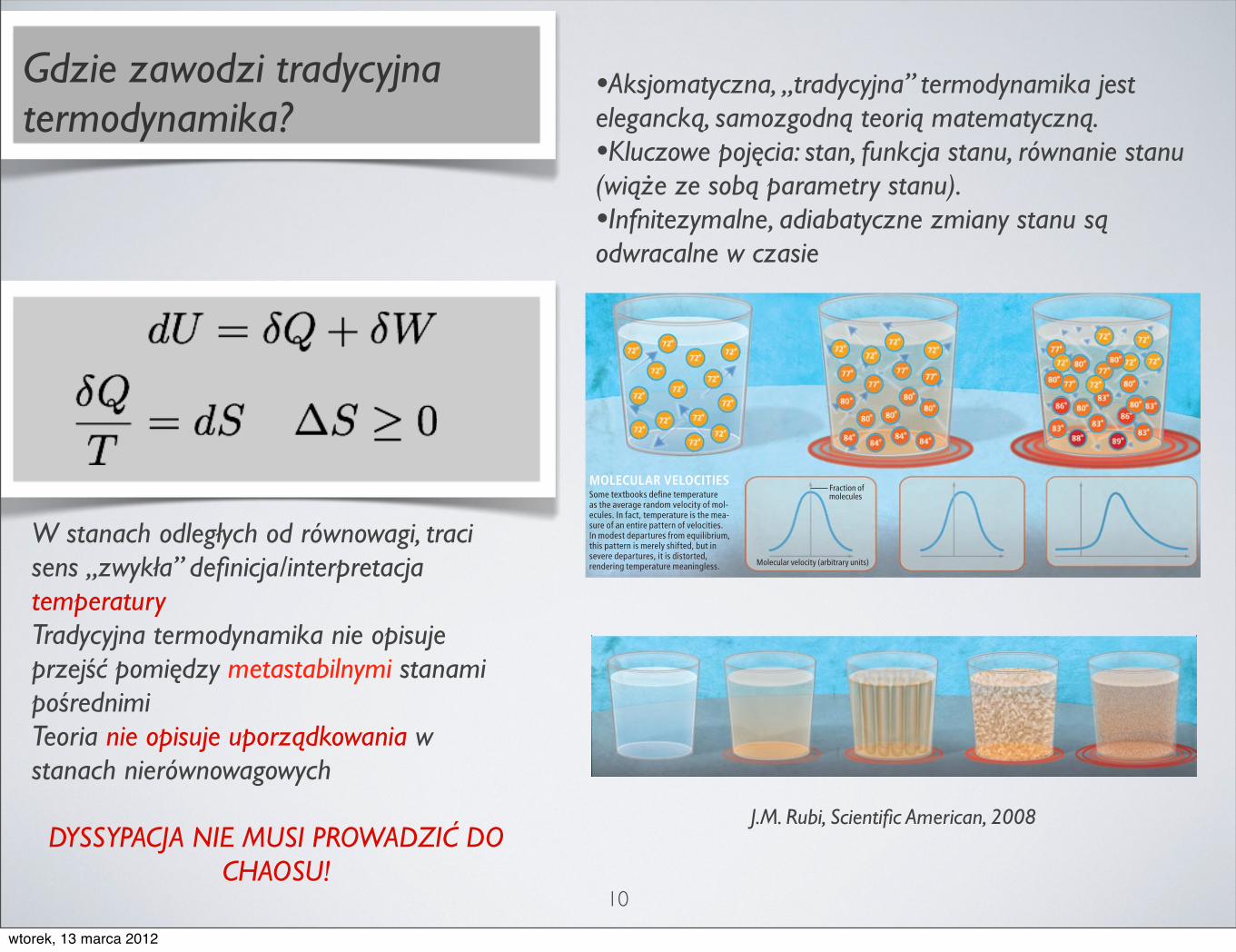
Gdzie zawodzi tradycyjna termodynamika?

J.M. Rubi, Scientific American, 2008

•Aksjomatyczna, „tradycyjna” termodynamika jest elegancką, samozgodną teorią matematyczną.•Kluczowe pojęcia: stan, funkcja stanu, równanie stanu(wiąże ze sobą parametry stanu).•Infnitezymalne, adiabatyczne zmiany stanu są odwracalne w czasie

W stanach odległych od równowagi, traci sens „zwykła” definicja/interpretacja temperaturyTradycyjna termodynamika nie opisuje przejść pomiędzy metastabilnymi stanami pośrednimiTeoria nie opisuje uporządkowania w stanach nierównowagowych

DYSSYPACJA NIE MUSI PROWADZIĆ DO CHAOSU!


11

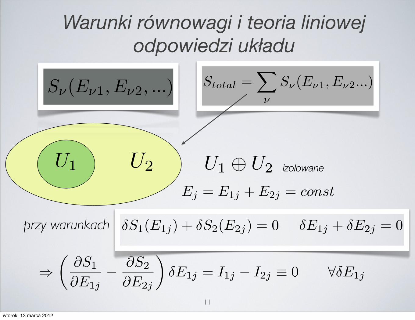
Warunki równowagi i teoria liniowej odpowiedzi układu

izolowaneU1 U2 U1 ⊕ U2

Ej = E1j + E2j = const

Sν(Eν1, Eν2, ...) Stotal =�

ν

Sν(Eν1, Eν2...)

przy warunkach δS1(E1j) + δS2(E2j) = 0 δE1j + δE2j = 0

⇒�

∂S1

∂E1j− ∂S2

∂E2j

�δE1j = I1j − I2j ≡ 0 ∀δE1j


POZA STANEM RÓWNOWAGI

12

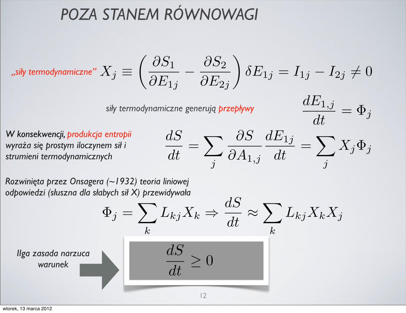
siły termodynamiczne generują przepływy

„siły termodynamiczne” Xj ≡�

∂S1

∂E1j− ∂S2

∂E2j

�δE1j = I1j − I2j �= 0

dE1,j

dt= Φj

dS

dt=

�

j

∂S

∂A1,j

dE1j

dt=

�

j

XjΦj

POZA STANEM RÓWNOWAGI

W konsekwencji, produkcja entropii wyraża się prostym iloczynem sił i strumieni termodynamicznych

Rozwinięta przez Onsagera (~1932) teoria liniowej odpowiedzi (słuszna dla słabych sił X) przewidywała

Φj =�

k

LkjXk ⇒ dS

dt≈

�

k

LkjXkXj

dS

dt≥ 0

IIga zasada narzuca warunek


13

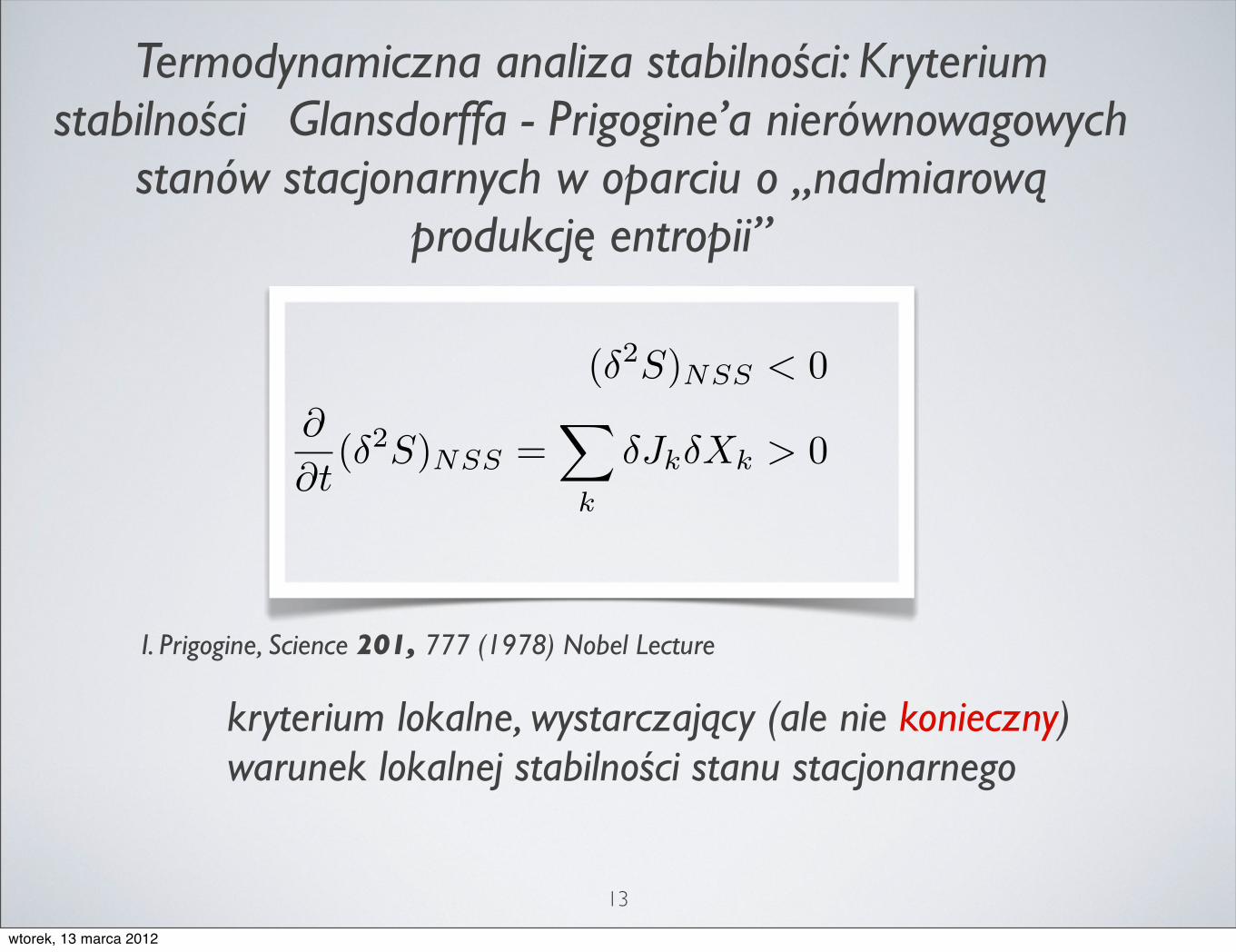
Termodynamiczna analiza stabilności: Kryterium stabilności Glansdorffa - Prigogine’a nierównowagowych

stanów stacjonarnych w oparciu o „nadmiarową produkcję entropii”

kryterium lokalne, wystarczający (ale nie konieczny) warunek lokalnej stabilności stanu stacjonarnego

(δ2S)NSS < 0

∂

∂t(δ2S)NSS =

�

k

δJkδXk > 0

I. Prigogine, Science 201, 777 (1978) Nobel Lecture


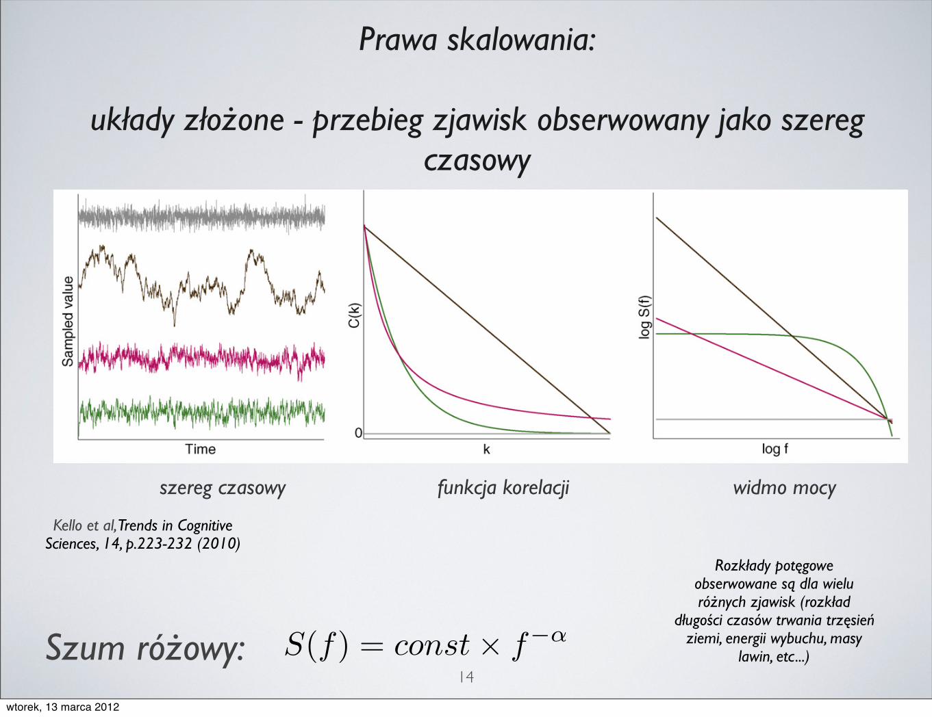
Prawa skalowania:

układy złożone - przebieg zjawisk obserwowany jako szereg czasowy

14envelope can be illustrated by tracing a line from peak topeak along a given waveform (i.e. the convex hull). Inter-estingly, the temporal scaling of amplitude fluctuations inongoing oscillations has recently been associated withcognitive impairments such as depression [66] and demen-tia [67]. Also, criticality has been supported bymultifractalpatterns in the same data previously supporting 1/f scaling[44]. Multifractal patterns occur when scaling relations(i.e. their exponents) vary over time or space, therebyadding a further dimension of complexity to data.

1/f scaling characterizes the central tendency of multi-fractal human performance, and thus the intrinsic fluctu-ations in neural and behavioral activity, be they from ionchannels or brain images or text sequences [55]. 1/f scalingsuggests that criticality underlies cognitive function atmultiple scales and levels of analysis. Although obser-vations of 1/f scaling in isolation do not constitute conclus-ive evidence for criticality (for other explanations, see Refs[3,68–70]), multifractal 1/f scaling greatly strengthens thecase [44]. Additionally, criticality predicts power-lawdistributions and pervasive temporal and spatial long-

range correlations in collective measures of componentactivities. These predictions are supported by the evidencereviewed here for neural avalanches [62], power-law distri-butions in word frequencies [33] and reaction times [28],and analyses showing pervasive 1/f scaling in neural [54]and behavioral activity [5] fluctuations. Adding multifrac-tality to the mounting evidence means that metastabilitynear critical points is the only candidate hypothesis thatcould explain the existing data.

Concluding remarksIn this brief review, a variety of scaling laws in cognitivescience were discussed that plausibly express adaptiveproperties of perception, action, memory, language andcomputation. The working hypothesis of criticality canprovide a general framework for understanding scalinglaws and has motivated the application of new analyticaltools to understand variability in cognitive systems. Muchwork lies ahead, however, to further test these newhypotheses and also to bring more scientists into thedebate (Box 3).

Box 2. Short-range versus long-range correlations

In physical systems, events occurring nearby in time or space areoften similar to each other, and such similarities typically fall off asdistance increases. Physicists use the correlation function to expressthe effect of distance on similarity, and the observed shape of thisfunction constitutes evidence about the type of system beingobserved.

To illustrate we use a characterization of the Ising model [77].Imagine a 2D grid of lights of varying brightness (from off tomaximum), where brightness is a function of two variables. One is arandom noise factor (individual to each light) and the other is aneighbor conformity factor whereby each light tends towards thebrightness of its four nearest neighbors on the grid. These twovariables are weighted together to determine the brightness of eachlight. In this illustration, the correlation function measures the degreeto which lights have equal brightness levels as a function of theirdistance apart on the grid. If noise is heavily weighted, then

brightness levels are independent across lights and the correlationfunction will be near zero for all distances >0. If instead neighborconformity is heavily weighted, then brightness levels will beinterdependent and approach uniformity, with a correlation functionnear one across a wide range of distances.Neither extreme is typical of physical systems. Instead, component

interactions are somewhere between independent and interdepen-dent. Weak interactions can result in short-range correlations (Figure Igreen) that decay exponentially with distance. Stronger interactionscan result in long-range correlations that decay more slowly (Figure Ipink) (i.e. as an inverse power of distance). The correlation functioncan also be defined for distances in time, with an analogouscomparison between weak (short-range) versus strong (long-range)interactions. No interactions can result in uncorrelated noise (Figure Igrey), and integrating over uncorrelated noise results in a randomwalk (Figure I brown).

Figure I. Four example time series are plotted in the left-hand panel: random samples from a normal distribution with zero mean and unit variance (i.e. whitenoise, in grey), a running sum of white noise (i.e. brown noise, also known as a random walk, in brown), 1/f noise (i.e. pink noise, in pink) and an autoregressivemoving average (ARMA, in green), where each sampled value is a weighted sum of a noise sample, plus the previous noise value, plus the previous sampledvalue. Idealized autocorrelation functions are shown in the middle panel for each of the time series, where k is distance in time. Note that white noise (i.e. pureindependence) has no correlations, ARMA has short-range correlations that decay exponentially with k, 1/f noise has long-range correlations that decay as aninverse power of k and brown noise has correlations that decrease linearly with k. Idealized spectral density functions (where f is frequency and S( f) is spectralpower) are shown in the right-hand panel in log–log coordinates. White, pink and brown noises correspond to straight lines with slopes of 0, !1 and !2, whereasARMA plateaus in the lower frequencies.

Review Trends in Cognitive Sciences Vol.xxx No.x

TICS-860; No. of Pages 10

7

szereg czasowy funkcja korelacji widmo mocy

Kello et al, Trends in Cognitive Sciences, 14, p.223-232 (2010)

Szum różowy: S(f) = const× f−α

Rozkłady potęgowe obserwowane są dla wielu różnych zjawisk (rozkład

długości czasów trwania trzęsień ziemi, energii wybuchu, masy

lawin, etc...)


15

Układy samoorganizujące się są dyssypatywne - charakteryzuje je pobór i straty energii

Uporządkowanie obejmuje całość układu, a dynamiczna zmienność jest zdeterminowana fluktuacjami parametrów kontrolnych

Układy samoorganizujące się cechuje wysoki stopień adaptacji do warunków zewnętrznych i wysoka odporność na zniszczenia


[...]Im głębiej analizujemy naturę czasu, tym lepiej rozumiemy, że trwanie oznacza inwencję, tworzenie form, stałe doskonalenie absolutnie „nowego”...

16

Czas jest iluzją...A. Einstein

Henri Bergson 1859-1941Nagroda Nobla 1927

Czas rzeczywisty (fizyczny) i czas subiektywny (durée)

[...]W naturze istnieje wielkość, która zmienia się w tym samym sensiewe wszystkich procesach naturalnych...Byłoby absurdem twierdzić, że zasada wzrostu entropii jest wynikiemnaukowej obserwacji, niedoskonałości eksperymentalnego pomiaru...

Max Planck 1858-1947Nagroda Nobla 1918

Niespójność? Determinizm mikroskopowych praw natury i kierunkowość zjawisk ewolucyjnych w przyrodzie


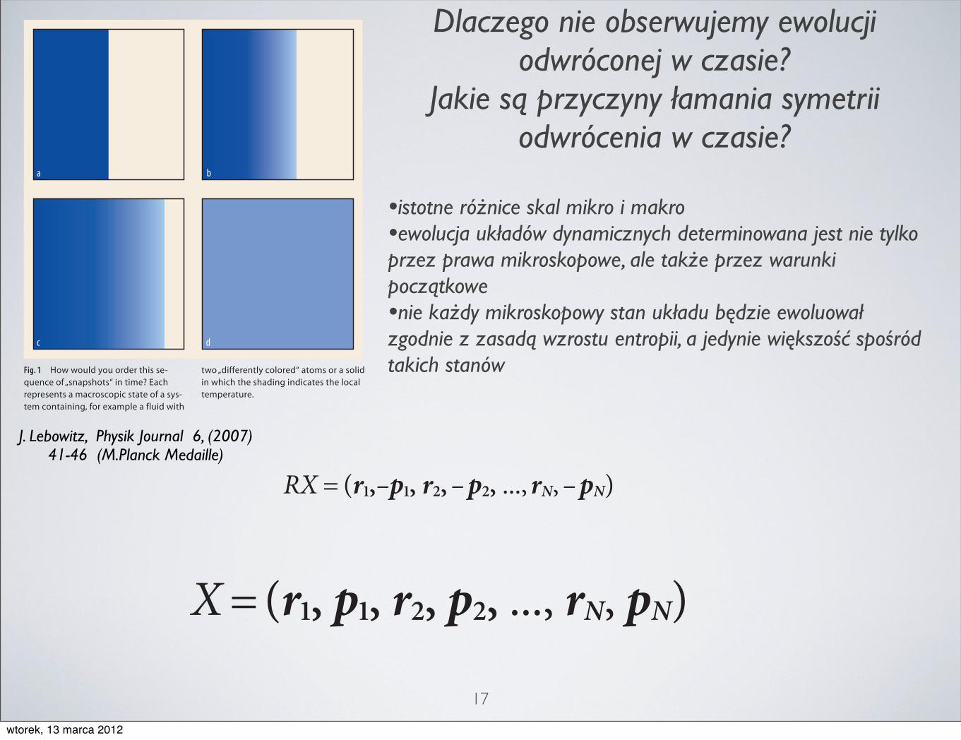
Dlaczego nie obserwujemy ewolucji odwróconej w czasie?

Jakie są przyczyny łamania symetrii odwrócenia w czasie?

•istotne różnice skal mikro i makro•ewolucja układów dynamicznych determinowana jest nie tylko przez prawa mikroskopowe, ale także przez warunki początkowe•nie każdy mikroskopowy stan układu będzie ewoluował zgodnie z zasadą wzrostu entropii, a jedynie większość spośród takich stanów

17

P R E I S T R Ä G E R

!" Physik Journal ! ("##$) Nr. %/& © !""# Wiley-VCH Verlag GmbH & Co. KGaA, Weinheim

Macroscopic Irreversibility: Problem and Resolution

In the world about us the past is distinctly different from the future. Milk spills but doesn’t unspill, eggs splatter but do not unsplatter, waves break but do not unbreak, we always grow older, never younger. These processes all move in one direction in time ! they are called „time-irreversible“ and define the arrow of time. It is therefore very surprising that the relevant fundamental laws of nature make no such distinction between the past and future. These laws permit all pro-cesses to be run backwards in time. This leads to a great puzzle ! if the laws of nature permit it why don‘t we observe the above mentioned processes run backwards? Why does a video of an egg splattering run backwards look ridiculous? Put another way: how can time-rever-sible motions of atoms and molecules, the microscopic components of material systems, give rise to observed time-irreversible behavior of our everyday world?

In the context of Newtonian theory, the „theory of everything“ at the time of Thomson, Maxwell and Boltzmann, the problem can be formally presented as follows: the complete microscopic (or micro) state of a classical system of N particles is represented by a point X in its phase space !,

X = (r!, p!, r", p", ..., rN, pN),

ri and pi being the position and momentum (or velo-city) of the ith particle. When the system is isolated, say in a box V with reflecting walls, its evolution is go-

verned by Hamiltonian dynamics with some specified Hamiltonian H(X) which we will assume for simplicity to be an even function of the momenta: no magnetic fields. Given H(X), the microstate X(t#), at time t#, determines the microstate X(t) at all future and past times t during which the system will be or was isolated: X(t) = Tt–t#X(t#). Let X(t#) and X(t# + "), with " posi-tive, be two such microstates. Reversing (physically or mathematically) all velocities at time t# + ", we obtain a new microstate. If we now follow the evolution for another interval " we find that the new microstate at time t# + "" is just RX(t#), the microstate X(t#) with all velocities reversed:

RX = (r!,–p!, r", – p", ..., rN, – pN).

Hence if there is an evolution, i. e. a trajectory X(t), in which some property of the system, specified by a function f (X(t)), behaves in a certain way as t increa-ses, then if f (X) = f (RX) there is also a trajectory in which the property evolves in the time reversed direc-tion.

Thus, for example, if the energy density or tem-perature inside the box V gets more uniform as time increases, e. g. in a way described by the diffusion equation, then, since the energy density profile is the same for X and RX, there is also an evolution in which the density gets more nonuniform. So why is one type of evolution, the one consistent with an entropy in-crease in accord with the „second law“, common and the other never seen? The difficulty is illustrated by the impossibility of time ordering of the snapshots in Fig. ! using solely the microscopic dynamical laws: the above time symmetry implies that if (a, b, c, d) is a possible ordering so is (d, c, b, a).

The explanation of this apparent paradox, due to Thomson, Maxwell and Boltzmann, as described in references [!!!"], shows that not only is there no conflict between reversible microscopic laws and irreversible macroscopic behavior, but, as clearly pointed out by Boltzmann in his later writings!), there are extremely strong reasons to expect the latter from the former. These reasons involve several interrelated ingredients which together provide the required distinction bet-ween microscopic and macroscopic variables and explain the emergence of definite time asymmetric behavior in the evolution of the latter despite the total absence of such asymmetry in the dynamics of the former. They are:! the great disparity between microscopic and macroscopic scales,! the fact that the events we observe in our world are determined not only by the microscopic dynamics, but also by the initial conditions of our system, which, if taken back far enough, inevitably lead to the initial conditions of our universe, and! the fact that it is not every microscopic state of a ma-croscopic system that will evolve in accordance with the entropy increase predicted by the second law, but only the „majority“ of such states ! a majority which however becomes so overwhelming when the number

!) Boltzmann‘s early writings on the subject are sometimes unclear, wrong, and even contra-dictory. His later wri-tings, however, are gene-rally very clear and right on the money (even if a bit verbose for Maxwell‘s taste. [#]) The presenta-tion here is not intended to be historical.

Fig. ! How would you order this se-quence of „snapshots“ in time? Each represents a macroscopic state of a sys-tem containing, for example a fluid with

two „differently colored“ atoms or a solid in which the shading indicates the local temperature.

a b

c d

J. Lebowitz, Physik Journal 6, (2007) 41-46 (M.Planck Medaille)






X = (r!, p!, r", p", ..., rN, pN),



RX = (r!,–p!, r", – p", ..., rN, – pN).







a b

c d






X = (r!, p!, r", p", ..., rN, pN),



RX = (r!,–p!, r", – p", ..., rN, – pN).







a b

c d


Termodynamiczna strzałka czasu wyznaczana procesami dyfuzji, wzrastającymi korelacjami i pojawieniem się zachowań kolektywnych w układach wielociałowych

Rozszerzenie teorii Poincaré: układy równań dynamicznych są niecałkowalne jeśli zawierają rezonanse pomiędzy rozmaitymi stopniami swobody

Rezonans: przejściowy stan metastabilny układu stwarzający możliwość efektywnego przekazu energii

18

The persistence of memory, S. Dali (1931)

W podejściu (filozofii) Szkoły Brukselskiej, kierunkowość czasu

jest podstawowym zjawiskiem wynikającym z dynamiki złożonych

układów fizycznych


Nurty współczesnej teorii układów złożonych (podejście synergetyczne) w naukach biologicznych (biologia systemów)

19

!"#$%&' ()*+,-. &/0

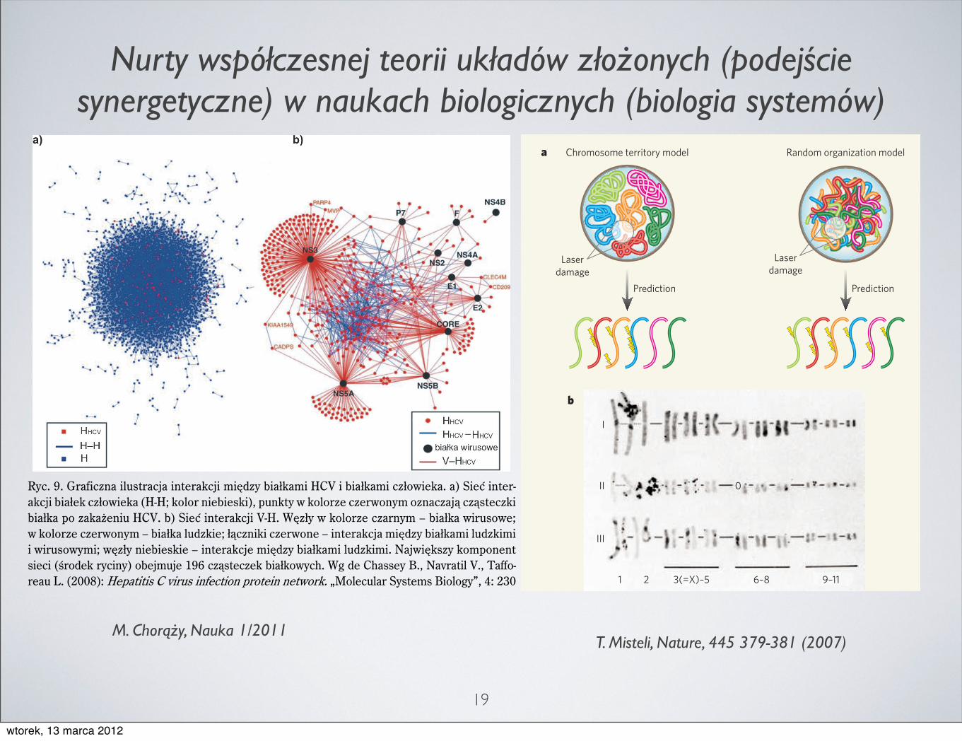
'%# $"1*)(."(234)*5#2-3&6-)&$,*7+8*6.%&3-$% *6.%&9 (:*%(;1.%# *6.%&61'%$%(<2"#"2:19-)(2&$,*;"( 9(="*>?@*"*>?AB*)".1'(*7+8C*(*%)" %(2&$,*6-3#2$D(<2"#*%*"2:19$D.(9(*) 3.-;&E*F;(*3#*;"( 9(*)&9(%1D *"23#.(9$D *%*9-=6<#9'#=*;"( #9*;"-. $&$,*1:%"()*(:,#%D"*9-=4.#9*:-*=($"#.%&*6-%(9-=4.9-)#DC*(*%*9-<#"*3#*%)" %(2#*%*(93&2(="*"*$&G3-'%9"#<#3#=*6# 2" * H129$D *)*=-;"<2- $"* "*="5.($D"*9-=4.#9E*I-%.#51<-)(2"#*3&$,H129$D"*6.%#%*;"( 9(*>?@*"*>?AB*=- #*6.-)(:%" *:-*%(;1.%# *=-;"<2- $"*9-=4.#9-:$%#6"#2"(*'" *"$,*-:*6-%(9-=4.9-)#D*=($"#.%&C*(*2('3 62"#*:-*%(6-$% 39-)(2"(*9(2G$#.-5#2#%&*"*6.-5.#'D"*2-)-3)-.1E

I&$E*JE*K.(H"$%2(*"<1'3.($D(*"23#.(9$D"*=" :%&*;"( 9(="*7+8*"*;"( 9(="*$% -)"#9(E*(L*?"# *"23#.G(9$D"*;"( #9*$% -)"#9(*M7G7N*9-<-.*2"#;"#'9"LC*61293&*)*9-<-.%#*$%#.)-2&=*-%2($%(D *$% '3#$%9";"( 9(*6-*%(9( #2"1*7+8E*;L*?"# *"23#.(9$D"*8G7E*O % &*)*9-<-.%#*$%(.2&=*P*;"( 9(*)".1'-)#N)*9-<-.%#*$%#.)-2&=*P*;"( 9(*<1:%9"#N* $%2"9"*$%#.)-2#*P*"23#.(9$D(*=" :%&*;"( 9(="*<1:%9"=""*)".1'-)&="N*) % &*2"#;"#'9"#*P*"23#.(9$D#*=" :%&*;"( 9(="*<1:%9"="E*>(D)" 9'%&*9-=6-2#23'"#$"*M .-:#9*.&$"2&L*-;#D=1D#*QJR*$% '3#$%#9*;"( 9-)&$,E*O5*:#*+,(''#&*SEC*>(T.(3"<*8EC*U(HH-G.#(1*VE*MW00/LX*7#6(3"3"'*+*T".1'*"2H#$3"-2*6.-3#"2*2#3)-.9E*Y!-<#$1<(.*?&'3#='*S"-<-5&ZC*[X*W@0

F$%#91D#*'" C* #*6-%2(2"#*(.$,"3#931.&*"*-54<2&$,*) ( $")- $"*'"#$"*9-=4.9-)&$,"*"23#.(9$D"*;"( 9-G;"( 9-*6-%)-<"*2(*;1:-)(2"#*1-54<2"-2&$,*,"6-3#%*-*=-<#91<(.2&$,6-:'3()($,* &$"(C*.-:%(D($,*.#51<($D"*#9'6.#'D"*5#24)C*"23#.(9$D"*=" :%&*6-:'"#$"(="C'3(;"<2- $"*"*#<('3&$%2- $"*'"#$"E*+#<#=*;"-<-5""*'&'3#=4)*D#'3*3(9 #*2-)(*9<('&H"9($D($,-.4;C*:"(52-'3&9(*"*3#.(6"(E*!- <")#C* #*1:(*'" *)'9(%( *3(9"#*) % &*"*6- $%#2"(*)*'"#G

M. Chorąży, Nauka 1/2011

Is the arrangement always the same, then?First of all, the patterns are probabilistic, rather than absolute; so although a chromosome may have a preferred average position in a cell population, the location of the chromosome in individual cells within that population can vary greatly. Even the two copies of the same chromosome within the same nucleus often occupy distinct positions and have different immediate neighbours.

Chromosome arrangements are also specific to the cell and tissue type, and can change during processes such as differentia-tion and development. For example, during

differentiation of immune T cells, mouse chro-mosome 6 moves from an internal position to the nuclear periphery.

The precise physiological relevance of chromosome positioning is currently unclear. However, its significance is hinted at by the fact that there is similarity in chromosome-position patterns among cell types that share common developmental pathways and by the observation that chromosome positions in a given cell type are evolutionarily con-served. For example, in human lymphocyte cells, chromosomes 18 and 19 tend to occupy a peripheral and an internal position, respectively — as does the corresponding

genetic material in Old World monkeys.

Why have all this organization?The nonrandom organization of the genome allows functional compartmentalization of the nuclear space. At the simplest level, active and inactive genome regions can be sepa-rated from each other, possibly to enhance the efficiency of gene expression or repres-sion. Such compartmentalization might also act in more subtle ways to bring co-regulated genes into physical proximity to coordinate their activities. For instance, in eukaryotes, the genes encoding ribosomal RNAs tend to cluster together in an organelle inside the nucleus known as the nucleolus. In addition, observations made in blood cells suggest that during differentiation co-regulated genes are recruited to shared regions of gene expression upon activation.

So, how do chromosomes find their place in the nucleus?We don’t know. Chromosomes are physically separated during cell division, but they tend to settle back into similar relative positions in the daughter cells, and then they remain stable throughout most of the cell cycle. So there must be some molecular mechanism that establishes and maintains the chromo-somes’ positions. The radial positioning of chromosomes has been related to either the chromosome gene density or the amount of DNA they contain, depending on cell type and proliferation status. But these cannot be the only factors involved, because the arrangement changes during differentiation and prolifera-tion, when gene density and chromosome size remain constant.

What are the mechanismsof chromosome positioning?There are two fundamentally different possi-bilities. It may be that chromosome positions are determined through their association with immobile nuclear elements — possibly a nuclear scaffold similar to the molecular structures that support and organize the cell’s cytoplasm. Although such anchoring may explain chromosome immobility and stabil-ity during the cell cycle, it cannot account for nonrandom positioning unless there is some sort of tethering mechanism that is specific to each chromosome and also encodes position-ing information.

An attractive alternative is a self-organiza-tion model in which the position of each chro-mosome is largely determined by the overall activity of all of its genes; that is, the number and pattern of active and silent genes on a given chromosome. The idea here is that the expres-sion status of a genome region affects local chromatin structure, with inactive regions being more condensed (heterochromatin) and highly active ones decondensed (euchro-matin). Depending on the degree of genome activity and the linear distribution of active and

At the turn of the twentieth century, Carl Rabl and Theodor Boveri proposed that each chromosome maintains its individuality during the cell cycle, and Boveri explained this behaviour in terms of ‘chromosome territories’.

The existence of chromosome territories was demonstrated experimentally during the early 1980s in pioneering microlaser experiments by the brothers Thomas and Christoph Cremer. They used a microlaser to induce local genome damage, and predicted that inflicting DNA damage within a small volume of the nucleus would yield different results depending on how chromosomes were arranged. If chromosomes

occupied distinct territories (a, left panel), localized damage would affect only a small subset of chromosomes, whereas if the chromatin fibres of each chromosome were randomly distributed throughout the nucleus (a, right panel), many chromosomes would be damaged. b, Three sets (I–III) of hamster chromosomes after laser damage. Only a subset of the chromosomes was damaged, as indicated by the black grains of radioactivity most prominently seen on chromosomes 1 and 2. This demonstrates the existence of chromosome territories. (Panel b was reprinted with permission from C. Zorn et al. Exp. Cell Res. 124, 111–119; 1979.) K.J.M. & T.M.

Box 1 | The discovery of chromosome territories

Prediction

Laserdamage

Laserdamage

Prediction

Chromosome territory modela Random organization model

b

III

0

1 3(=X)–5 6–8 9–112

II

I

380

NATURE|Vol 445|25 January 2007NEWS & VIEWS Q&A

T. Misteli, Nature, 445 379-381 (2007)


Podsumowanie i „luźne” wątki...

20

Powszechność układów złożonych i zjawisk samoorganizacji czasowo-przestrzennej w różnych skalach obserwacji przyrody (od biologii po

kosmologię..) sugeruje, że zrozumienie charakteru „praw” , mechanizmów odpowiedzialnych za „samoporządkowanie” i spontaniczne powstawanie

struktur może być kluczem do spójnego opisu materii.

Czy (nieliniowa) dynamika, przyczynowość i przypadek (fluktuacje) są wystarczającymi elementami tego opisu?


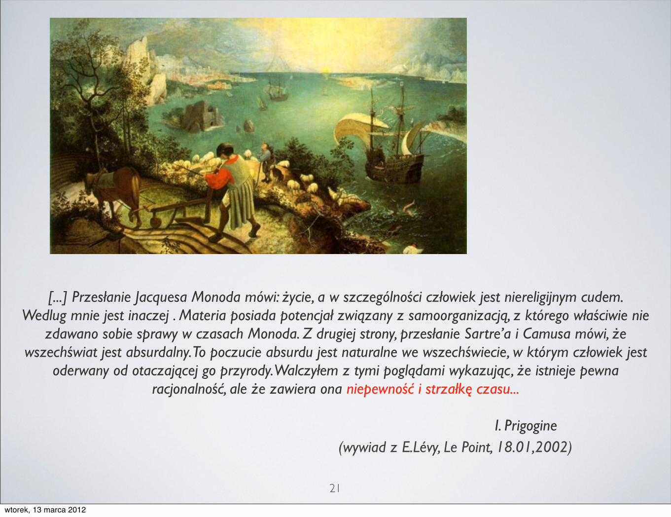
[...] Przesłanie Jacquesa Monoda mówi: życie, a w szczególności człowiek jest niereligijnym cudem.Wedlug mnie jest inaczej . Materia posiada potencjał związany z samoorganizacją, z którego właściwie nie

zdawano sobie sprawy w czasach Monoda. Z drugiej strony, przesłanie Sartre’a i Camusa mówi, że wszechświat jest absurdalny. To poczucie absurdu jest naturalne we wszechświecie, w którym człowiek jest

oderwany od otaczającej go przyrody. Walczyłem z tymi poglądami wykazując, że istnieje pewna racjonalność, ale że zawiera ona niepewność i strzałkę czasu...

I. Prigogine

21

(wywiad z E.Lévy, Le Point, 18.01,2002)


22

Dziękuję za uwagę

Plus ratio quam vis


paradygmaty ewolucji naukowo-kulturalnej w pracach ilyi...

Documents