parallel algorithm for learning optimal bayesian...

Journal of Machine Learning Research 12 (2011) 2437-2459 Submitted 7/10; Revised 2/11; Published 7/11

Parallel Algorithm for Learning Optimal Bayesian Network Structure

Yoshinori Tamada∗ TAMADA @IMS.U-TOKYO.AC.JP

Seiya Imoto [email protected]

Satoru Miyano† MIYANO @IMS.U-TOKYO.AC.JP

Human Genome CenterInstitute of Medical Science, The University of Tokyo4-6-1 Shirokanedai, Minato-ku, Tokyo 108-8639, Japan

Editor: Russ Greiner

AbstractWe present a parallel algorithm for the score-based optimalstructure search of Bayesian networks.This algorithm is based on a dynamic programming (DP) algorithm havingO(n · 2n) time andspace complexity, which is known to be the fastest algorithmfor the optimal structure search ofnetworks withn nodes. The bottleneck of the problem is the memory requirement, and therefore,the algorithm is currently applicable for up to a few tens of nodes. While the recently proposedalgorithm overcomes this limitation by a space-time trade-off, our proposed algorithm realizes di-rect parallelization of the original DP algorithm withO(nσ) time and space overhead calculations,whereσ > 0 controls the communication-space trade-off. The overalltime and space complexity isO(nσ+12n). This algorithm splits the search space so that the requiredcommunication between in-dependent calculations is minimal. Because of this advantage, our algorithm can run on distributedmemory supercomputers. Through computational experiments, we confirmed that our algorithmcan run in parallel using up to 256 processors with a parallelization efficiency of 0.74, comparedto the original DP algorithm with a single processor. We alsodemonstrate optimal structure searchfor a 32-node network without any constraints, which is the largest network search presented inliterature.

Keywords: optimal Bayesian network structure, parallel algorithm

1. Introduction

A Bayesian network represents conditional dependencies among random variables via a directedacyclic graph (DAG). Several methods can be used to construct a DAG structure from observeddata, such as score-based structure search (Heckerman et al., 1995; Friedman et al., 2000; Imotoet al., 2002), statistical hypothesis testing-based structure search (Pearl, 1988), and a hybrid ofthese two methods (Tsamardinos et al., 2006). In this paper, we focus on ascore-based learningalgorithm and formalize it as a problem to search for an optimal structure thatderives the maximal(or minimal) score using a score function defined on a structure with respect to an observed data set.A score function has to be decomposed as the sum of the local score functions for each node in anetwork. In general, posterior probability-based score functions derived from Bayesian statistics areused. The optimal score-based structure search of Bayesian networks is known to be an NP-hard

∗. Currently at Department of Computer Science, Graduate School of Information Science and Technology, The Uni-versity of Tokyo. 7-3-1 Hongo, Bunkyo-ku, Tokyo 113-0033, Japan. [email protected].

†. Also at the Computational Science Research Program, RIKEN, 2-1 Hirosawa, Wako, Saitama 351-0198, Japan.

c©2011 Yoshinori Tamada, Seiya Imoto and Satoru Miyano.

TAMADA , IMOTO AND M IYANO

problem (Chickering et al., 1995). Several efficient dynamic programming (DP) algorithms havebeen proposed to solve such problems (Ott et al., 2004; Koivisto and Sood, 2004). Such algorithmshaveO(n ·2n) time and space complexity, wheren is the number of nodes in the network. Whenthese algorithms are applied to real problems, the main bottleneck is bound to be the memoryspace requirement rather than the time requirement, because these algorithmsneed to store theintermediate optimal structures of all combinations of node subsets during DP steps. Because ofthis limitation, such algorithm can be applied to networks of only up to around 25 nodes in a typicaldesktop computer. Thus far, the maximum number of nodes treated in an optimalsearch withoutany constraints is 29 (Silander and Myllymaki, 2006). This was realized by using a 100 GB externalhard disk drive as the memory space instead of using the internal memory, which is currently limitedto only up to several tens of GB and in a typical desktop computer.

To overcome the above mentioned limitation, Perrier et al. (2008) proposed an algorithm toreduce the search space using structural constraints. Their algorithm searches for the optimal struc-ture on a given predefined super-structure, which is often available in actual problems. However, itis still important to search for a globally optimal structure because Bayesian networks find a widerange of applications. As another approach to overcome the limitation, Parviainen and Koivisto(2009) proposed a space-time trade-off algorithm that can search fora globally optimal structurewith less space. From empirical results for a partial sub-problem, they showed that their algorithmis computationally feasible for up to 31 nodes. They also mentioned that their algorithm can beeasily parallelized with up to 2p processors, wherep = 0,1, . . . ,n/2 is a parameter that is used tocontrol the space-time trade-off. Using parallelization, they suggested that it might be possible tosearch larger-scale network structures using their algorithm. The time and space complexities oftheir algorithm areO(n·2n(3/2)p) andO(n·2n(3/4)p), respectively.

Of course, the memory space limitation can be overcome by simply using a computerwith suf-ficient memory. The DP algorithm remains computationally feasible even for a 29-node networkin terms of the time requirement. For such a purpose, a supercomputer with shared memory isrequired. Modern supercomputers can be equipped with several terabytes of memory space. There-fore, they can be used to search larger networks than the current 29-node network that requires 100GB of memory. However, such supercomputers are typically very expensive and are not scalable interms of the memory size and the number of processors. In contrast, massively parallel computers,a much cheaper type of supercomputers, make use of distributed memory; in such systems manyindependent computers or computation nodes are combined and linked through high-speed connec-tions. This type of supercomputers is less expensive, as mentioned, and itis scalable in terms ofboth the memory space and the number of processors. However the DP algorithm cannot be exe-cuted on such a distributed memory computer because it requires memory access to be performedover a wide region of data, and splitting the search space across distributed processors and storingthe intermediate results in the distributed memory are not trivial problems.

Here, we present a parallelized optimal Bayesian network search algorithm calledPara-OS. Theproposed algorithm is based on the OS algorithm using DP that was proposed by Ott et al. (2004).Our algorithm realizes direct parallelization of the DP steps in the original algorithm by splittingthe search space of DP withO(nσ) time and space overhead calculations, whereσ = 1,2, . . . > 0is a parameter that is used to split the search space and controls the trade-off between the numberof communications (not the volume of communication) and the memory space requirement. Themain feature of this algorithm is that it guarantees that the amount of intermediateresults that are re-quired to be shared redundantly among independently split calculations is minimal. In other words,

2438

PARALLEL ALGORITHM FOR LEARNING OPTIMAL BAYESIAN NETWORKS

our algorithm guarantees that minimal communications are required between independent parallelprocessors. Because of this advantage, our algorithm can be easily parallelized, and, in practice, itcan run very efficiently on massively parallel computers with several hundreds of processors. An-other important feature of our algorithm is that it calculates no redundant score functions, and itcan distribute the entire calculation almost equally across all processors. The main operation in ouralgorithm is the calculation of the score function. In practice, this feature is important to actuallysearch for the optimal structure. The overall time and space complexity isO(nσ+12n). Our algorithmadopts an approach opposite to that of Parviainen and Koivisto (2009) toovercome the bottleneckof the memory space problem. Although our algorithm has slightly greater space and time com-plexties, it makes it possible to realize large-scale optimal network search in practice using widelyavailable low-cost supercomputers.

Through computational experiments, we show that our algorithm is applicableto large-scaleoptimal structure search. First, the scalability of the proposed algorithm to thenumber of proces-sors is evaluated through computational experiments with simulated data. We confirmed that theprogram can run efficiently in parallel using up to 256 processors (CPUcores) with a paralleliza-tion efficiency of more than 0.74 on a current supercomputer system, and acceptably using up to512 processors with a parallelization efficiency of 0.59. Finally, we demonstrate the largest optimalBayesian network search attempted thus far on a 32-node network with 256processors using ourproposed algorithm without any constraints and without an external harddisk drive. Our algorithmwas found to complete the optimal search including the score calculation within a week.

The remainder of this paper is organized as follows. Section 2 presents anoverview of theBayesian network and the optimal search algorithm, which serves as the basis for our proposedalgorithm. Section 3 describes the parallel optimal search algorithm in detail. Section 4 describesthe computational experiments used for evaluating our proposed algorithm and presents the obtainedresults. Section 5 concludes the paper with a brief discussion. The appendix contains some proofsand corollaries related to those described in the main paper.

2. Preliminaries

In this section, we first present a brief introduction to the Bayesian network model, and then, wedescribe the optimal search (OS) algorithm, which is the basal algorithm that we parallelize in theproposed algorithm.

2.1 Bayesian Network

A Bayesian network is a graphical model that is used to represent a joint probability of random vari-ables. By assuming the conditional independencies among variables, the joint probability of all thevariables can be represented by the simple product of the conditional probabilities. These indepen-dencies can be represented via a directed acyclic graph (DAG). In a DAG, each node corresponds toa variable and a directed edge, to the conditional dependencies among variables or to the indepen-dencies from other variables. Suppose that we haven random variables,V = {X1,X2, . . . ,Xn}. Thejoint probability of variables inV is represented as

P(X1,X2, . . . ,Xn) =n

∏j=1

P(Xj |PaG(Xj)),

2439


wherePaG(Xj) represents the set of variables that are direct parents of thej-th variableXj in networkstructureG andP(Xj |PaG(Xj)), a conditional probability for variableXj .

A score-based Bayesian network structure search or a Bayesian network estimation problem isto search for the DAG structure fitted to the observed data, in which the fitness of the structure to thegiven data is measured by a score function. The score function is defined on a node and its parentset. The scores of nodes obtained by a score function are called local scores. A network score isdefined simply as the sum of local scores of all nodes in a network. Using ascore function, theBayesian network structure search can be defined as a problem to find anetwork structureG thatsatisfies the following equation:

G= argminG

n

∑j=1

s(Xj ,PaG(Xj),X),

wheres(Xj ,PaG(Xj),X) is a score functions : V×2V ×RN,n→ R for nodeXj given the observed

input data of an(N×n)-matrixX, whereN is the number of observed samples.

2.2 Optimal Search Algorithm using Dynamic Programming

Next, we briefly introduce the OS algorithm using DP proposed by Ott et al. (2004). Our proposedalgorithm is a parallelized version of this algorithm. We employ score functions described as in theoriginal paper by Ott et al. (2004). That is, a smaller score representsbetter fitting of the model.Therefore, the problem becomes one of finding the structure that minimizes the score function. Theoptimal network structure search by DP can be regarded as an optimal permutation search problem.The algorithm consists of two-layer DP: one for obtaining the optimal choice of the parent setfor each node and one for obtaining the optimal permutation of nodes. First,we introduce somedefinitions.

Definition 1 (Optimal local score) We define the function F: V×2V → R as

F(v,A)def= min

B⊂As(v,B,X).

That is, F(v,A) calculates the optimal choice of the parent set from A for node v and returns itsoptimal local score. B⊂ A represents the actual optimal choice for v, and generally, we also needto include it in the algorithm along with the score, in order to reconstruct the network structurelater.

Definition 2 (Optimal network score on a permutation) Let π : {1,2, . . . , |A|} → A be a permu-tation on A⊂ V andΠA be a set of all the permutations on A. Given a permutationπ ∈ ΠA, theoptimal network score onπ can be described as

QA(π) def= ∑

v∈A

F(v,{u∈ A : π−1(u)< π−1(v)}).

Definition 3 (Optimal network score) By using QA(π) defined above, we can formalize the net-work structure search as a problem to find the optimal permutation that gives the minimal networkscore:

M(A)def= arg min

π∈ΠAQA(π).

2440


Here,M(A) represents the optimal permutation that derives the minimal score of the network con-sisting of nodes inA.

Finally, the following theorem provides an algorithm to calculateF(v,A), M(A), andQA(M(A))by DP. See Ott et al. (2004) for the proof of this theorem.

Theorem 4 (Optimal network search by DP) The functions F(v,A), M(A), and QA(M(A)) de-fined above can be respectively calculated by the following recursive formulae:

F(v,A) = min{s(v,A,X),mina∈A

F(v,A\{a})}, (1)

M(A)(i) =

{

M(A\{v∗})(i) (i < |A|)v∗ (i = |A|)

, (2)

QA(M(A)) = F(v∗,A\{v∗})+QA\{v∗}(M(A\{v∗})), (3)

wherev∗ = argmin

v∈A{F(v,A\{v})+QA\{v}(M(A\{v}))}.

By applying the above equations from|A|= 0 to |A|= |V|, we obtain the optimal permutationπ onV and its score QV(M(V)) in O(n·2n) steps.

Note that in order to reconstruct the network structure, we need to keep the optimal choice ofthe parent set derived in Equation (1) and the optimal permutationπ = M(A) in Equation (3) for allthe combinations ofA⊂V in an iterative loop for the next size ofA.

3. Parallel Optimal Search Algorithm

The key to parallelizing the calculation of the optimal search algorithm by DP is splitting all thecombinations of nodes in a single loop of DP forF(v,A), M(A), andQA(M(A)), given above byEquations (1), (2), and (3), respectively. Simultaneously, we need to consider how to reduce theamount of information that needs to be exchanged between processors.In the calculation ofM(A),we need to obtain all the results ofM(·) for one-smaller subsets ofA at hand, that is,M(A\ {a})for all a∈ A. Suppose that suchM(A\ {a})’s are stored in the distributed memory space, and wehave collected them for calculatingM(A). In order to reduce the number of communications, itwould be better if we can re-use the collected results for another calculation. For example, we cancalculateM(B) (|B|= |A|) in the same processor that calculatesM(A) such that some ofM(B\{b})(b∈ B) overlaps M(A\ {a}). That is, if we can collect the maximal number ofM(X)’s for anyXsuch that|X|= |A|−1∧ X ⊂ {(A\{a})∩ (B\{b})}, then the number of communications requiredfor calculatingM(A) andM(B) can be minimized. Theorem 7 shows how we generate such a set ofcombinations, and we prove that it provides the optimally minimal choice of such combinations byallowing some redundant calculations.

In addition, as is evident from Equations (1), (2), and (3), the DP algorithm basically consistsof simply searching for the best choice from the candidates that derive the minimal score. Timeis mainly required to calculate the score functions(v,A,X) for all the nodes and their parent com-binations. Thus, our algorithm calculatess(v,A,X) equally in independent processors without anyredundant calculations for this part.

In this section, we first describe some basic definitions, and then, we present proofs of theoremsthat the proposed algorithm relies on. Finally, we present the proposed parallel algorithm.

2441


3.1 Separation of Combinations

First, we define the combination, sub-combination, and super-combination ofnodes.

Definition 5 (Combination) In this paper, we refer to a set of nodes in V as a combination of nodes.We also assume a combination of k nodes, that is, X= {x1,x2, . . . ,xk} ⊂ V such that ord(xi) <ord(x j) if i < j, where ord: V → N is a function that returns the index of element v∈ V. Forexample, suppose that V= {a,b,c,d}. ord(a) = 1 and ord(d) = 4.

Definition 6 (Sub-/super-combination) We define C′ as a sub-combination of some combinationC if C′ ⊂C, and C is a super-combination of C′. We say that a super-combination C is generatedfrom C′ if C is a super-combination of C′. In addition, we say that sub-combination C′ is derivedfrom C if C′ is a sub-combination of C. For the sake of convenience, if we do not mention aboutthe size of a sub-/super-combination of a combination, then we assume that it refers to a one-sizesmaller/larger sub-/super-combination. In addition, we say that two combinations A and B sharesub-combinations ifA ′∩B ′ 6= /0, whereA ′ andB ′ are sets of all the sub-combinations of A and B,respectively.

We present two theorems that our algorithm relies on along with their proofs.These two theo-rems are used to split the calculation ofF(v,A), M(A), andQA(M(A)); all these require the resultsfor their sub-combinations. We show that the calculation can be split by the super-combination ofA, and it is the optimal separation of the combinations in terms of the number of communicationsrequired.

Theorem 7 (Minimality of required sub-combinations) LetA be a set of combinations of nodesin V , where|A|= k> 0 for A∈A and|V|= n. If |A |=

(k+σk

)

(σ > 0∧ σ+k≤ n), then the minimal

number of sub-combinations of length k−1 required to generate all the combinations inA is(k+σ

k−1

)

.Let S be a combination of nodes, where|S|= k+σ. We can generate a set of combinations of lengthk that satisfies the former condition by deriving all the sub-combinations of length k from S.

Proof BecauseA contains(k+σ

k

)

combinations of lengthk, the number of distinct elements (nodes)involved inA is k+σ and is minimal. Therefore, the number of sub-combinations required to derive(k+σ

k

)

combinations of lengthk in A is equal to the number of possible combinations that can begenerated fromk+σ elements, and is

(k+σk−1

)

. No more combinations can be generated from(k+σ

k−1

)

sub-combinations. Therefore, it is the minimal number of required sub-combinations required togenerate

(k+σk

)

combinations. A super-combinationSof lengthk+σ containsk+σ elements andcan derive

(k+σk

)

combinations of lengthk. Therefore,Scan deriveA , and all the combinations oflengthk−1 derived from elements inSare the sub-combinations required to generate combinationsin A .

Theorem 8 (Minimality of required super-combinations) The minimal number ofsuper-combinations of length k+σ from V that is required to generate all the sub-combinationsof size k is

(n−σk

)

.

2442


Proof Consider the setT = V \ {v1,v2, . . . ,vσ}, where anyvi ∈ V, and thus,|T| = n−σ. If wegenerate all the combinations of lengthk taken fromT, then these include all the combinations oflengthk from nodes inV without v1, . . . ,vσ, and the number of combinations is

(n−σk

)

. Consider aset of combinationsS = {{v1, . . . ,vσ}∪T ′ : T ′ ⊂ T ∧ |T ′| = k}. Here,|S| = k+σ for S∈ S and|S | =

(n−σk

)

. BecauseS contains all the combinations of lengthk without v1, . . . ,vσ and all theelements inS containv1, . . . ,vσ, we can generate all the combinations inV of lengthk from someS∈ S by combining 0≤ α ≤ k nodes fromv1, . . . ,vσ and k−α nodes fromS\ {v1, . . . ,vσ}. Ifwe remove anyS∈ S from it, then there exist combinations that cannot be generated from anotherS∈ S becauseS lists all the combinations except for nodesv1, . . . ,vσ. Therefore,S is the minimalset of super-combinations required to derive all the combinations of lengthk from V and its sizeis |S | =

(n−σk

)

. We can generateS by taking the first(n−σ

k

)

combinations from(n

k

)

combinationsarranged in lexicographical order.

Theorem 7 can be used to split the search space of DP using bysuper-combinations, and Theo-rem 8 provides the number of super-combinations required in the parallel computation for a certainsize ofA for M(A). From these two theorems, we can easily derive the following corollaries.

Corollary 9 (Optimal separation of combination) The DP steps used to calculate M(A) andQA(M(A)) in the OS algorithm can be split into

(n−σk

)

portions by super-combinations of A with

length k+σ, where|A| = k. The size of each split problem is(k+σ

k

)

and the number of required

M(B) for B⊂ A ∧ |B| = k− 1 is(k+σ

k−1

)

, which is the minimal number for(k+σ

k

)

combinations ofM(A). Here, B is a set of sub-combinations of A. The calculation of F(v,A) can also be split basedon the sub-combinations B for M(A).

The separation ofM(A) by super-combinations causes some redundant calculations. The fol-lowing corollary gives the amount of such overhead calculations and the overall complexity of thealgorithm.

Corollary 10 (Amount of redundant calculations) If we split the calculations of M(A) (|A| = k)using super-combinations of size k+σ (σ > 0), then the number of calculations of M(A) for allA⊂V is

(n−σk

)

·(k+σ

k

)

=(n

k

)

O(nσ). Thus, as compared to the original DP steps(n

k

)

, the overheadincrement of the calculations for M(A),QA(M(A)), and F(v,A) is at most O(nσ). The memory re-quirement to store the intermediate results is also dependent on the size of the sub-combinations forsplit calculations. Therefore, the overall time and space complexity of the algorithm is O(nσ+12n).

We present a proof in Appendix B. The parameterσ > 0 can be used to control the size of splitproblems. Because using a large value ofσ suppresses the number of required super-combinations,the number of communications required between independent calculations is also suppressed. In-stead, the large value ofσ requires a large memory space to store the sub-combinations in a pro-cessor. Therefore,σ can be used to control the trade-off between the number of communicationsand the memory space requirement. Because the algorithm requires the exchange of intermediateresults

(n−σk

)

times for a loop with|A| = k and is a relatively large number, decreasing the numberof communications reduces the communication speed. In a case with many processors, however,a large value ofσ can also reduce the communication speed because a large value ofσ requiresthe transfer of a large amount of data, instead of reducing the number of communications. Table 1

2443


Increment fork σ = 1 σ = 2 σ = 31 1 2 32 2 5 8

10 7 30 5514 8 37 11127 4 8 8

Table 1: Examples of the actual increment of various values ofk andσ for n= 32. The incrementis largest for all cases ofσ for k= 14.

Algorithm 1 Process-S(S,a,n,np) calculates the functionsF(v,A), M(A), andQA(M(A)) for com-binationsA derived from the given super-combinationS.Input: S⊂V : Super-combination,a∈N : size of combination to be calculated,n: total number of

nodes in the network,np : number of CPU processors (cores).Output: F(v,B), Q(A), andM(Q(A)) for all sub-combinations ofS with sizea, v ∈ A, andB =

A\{v}.1: A ←{A⊂ S: |A|= a}2: Retrieve the local scoress(v,B,X) for B= A\{v} (v∈ A∈ A) from theLF(v,B,n,np)-th pro-

cessor.3: RetrieveF(u,B\{u}) for u∈ B (B= A\{v},v∈ A∈ A) from theLF(u,B\{u},n,np)-th pro-

cessor.4: RetrieveQA\{v}(M(A\{v})) for v∈ A∈ A from theLQ(A\{v},n,np)-th processor.5: for eachA∈ A do6: CalculateF(v,B) for v ∈ A,B = A\ {v} from s(v,B) andF(v,B\ {u}) for u ∈ B by Equa-

tion (1).7: CalculateM(A) andQA(M(A)) from QA\{v}(M(A\{v})) andF(v,A\{v}) by Equations (3)

and (2).8: end for9: StoreQ(A) andMA(Q(A)) (A∈ A) in theLQ(A,n,np)-th processor.

10: StoreF(v,B) (B= A\{v},A∈ A) in theLF(v,B,n,np)-th processor.

shows some examples of the actual overhead increment of the DP steps, that is,(n−σ

k

)

·(k+σ

k

)

/(n

k

)

.As shown in the table, the increment because of redundant DP steps caused by the separation ap-pears to be relatively small for a case of the practical size ofn andσ. If the algorithm runs in parallelwith hundreds of processors, the increment calculation in each processor is negligible as comparedto the total amount of calculations, and thus, it does not noticeably affect the overall computationtime. We discuss this later with the computational experiments presented in Section 4.2.

2444


Algorithm 2 Para-OS(V,X,s,σ,np) calculates the exactly global optimal structure of the Bayesiannetwork with respect to the input dataX and the local score functionswith np processors.

Input: V: set of input nodes (variables) where|V| = n, X: (N×n)-input data matrix,s(v,Pa,X):functionV×2V ×R

N×n→ R that returns the local Bayesian network score for variablev withits parent setPa⊂ V w.r.t. the input data matrixX, σ ∈ N: size of super-combination,np:number of CPU processors (cores).

Output: G= (V,E) : optimal Bayesian network structure.1: {Initialization}2: CalculateF(v, /0) = s(v, /0,X) for all v∈V and store it in theLF(v, /0,n,np)-th processor.3: StoreF(v, /0) asQ{v}(M({v})) andM({v})(1) = v for all v∈V in theLQ({v},n,np)-th proces-

sor.4: {Main Loop for size ofA}5: for a= 1 ton−1 do6: {S-phase: Execute the following for-loop oni in parallel. The{r = i modnp+1}-th proces-

sor is responsible for the(i+1)-th loop.}7: for i = 0 ton

(n−1a

)

−1 do8: v← i modn+19: j ← ⌊i /n⌋+1

10: Pa←m(v,RLI−1( j,n−1,a))11: Calculates(v,Pa,X) and store it in the local memory of ther-th processor.12: end for13: {Q-phase: Execute the following for-loop oni in parallel. The{r = i modnp+1}-th pro-

cessor is responsible for the(i+1)-th loop.}14: if a+σ+1> n then15: σ← n−a−1.16: end if17: for i =

( na+σ+1

)

−(n−σ

a+1

)

to( n

a+σ+1

)

−1 do18: S← RLI−1(i+1,n,a+σ+1).19: Call Process-S(S,a+1,n,np).20: end for21: end for22: Construct networkG = (V,E) by collecting the final sets of the parents selected in line 6 of

Process-S(·).23: return G= (V,E).

3.2 Para-OS Algorithm

According to Theorems 7 and 8 and Corollary 9, the DP steps in Equations (1), (2), and (3) ofTheorem 4 can be split by super-combinations ofA. The pseudocode of the proposed algorithm isgiven by Algorithms 1 and 2. The former is a sub-routine of the latter main algorithm.

The algorithm consists of two phases: the S-phase and the Q-phase. In the former, each pro-cessor calculates the score functions(v,Pa,X) independently without communication, whereas thelatter calculatesF(v,A), M(A), andQA(M(A)) along with communications among each other toexchange the results ofF(v,A), M(A), andQA(M(A)). Note that in line 6 of Algorithm 1, we need

2445


to store not only the local scores but also the optimal choices of parent node sets, although we donot describe this explicitly. This is required to reconstruct the optimal structure after the algorithmterminates.

In this algorithm, we need to determine which processor stores the calculated intermediate re-sults. In order to calculate this, we define some functions as given below.

Definition 11 We define function m′ : N×N→ N as follows:

m′(a,b) =

{

a if a< ba+1 otherwise

.

Using m′(a,b), we define function m: V×2V → 2V as follows:

m(v,A) = {ord−1(m′(ord(u),ord(v))) : u∈ A}.

In addition, we define function m′−1 : N×N→ N as follows:

m′−1(a,b) =

{

a if a< ba−1 otherwise

.

Using m′−1(a,b), we define function m−1 : V×2V → 2V as follows:

m−1(v,A) = {ord−1(m′−1(ord(u),ord(v))) : u∈ A}.

The functionm(v,A) maps the combinationA to a new combination inV \{v}, andm−1(v,A) is theinverse function ofm(v,A). These are used in the proposed algorithm and the following function.

Definition 12 (Calculation of processor index to store and retrieve results) We define functionsLQ : 2V ×N×N→ N and LF : V×2V ×N×N→ N as follows:

LQ(A,n,np)def= (RLI(A,n)−1) modnp+1

andLF(v,A,n,np)

def=

{

(RLI(m−1(v,A),n−1)−1)×n+(ord(v)−1)}

modnp+1,

where RLI(A,n) is a function used to calculate the reverse lexicographical index (RLI) of combina-tion A taken from n objects and np, the number of processors.

FunctionLQ(A,n,np) locates the processor index used to store the results ofM(A) andQA(M(A))and LF(v,A,n,np), the results ofF(v,A). By using RLIs, the algorithm can independently anddiscontinuously generate the required combinations and processor indices for storing/retrieving ofintermediate results. We use RLIs instead of ordinal lexicographical indices because the conversionbetween a combination and the RLI can be calculated in linear time by preparing the index tableonce (Tamada et al., 2011). In Algorithm 2, the inverse functionRLI−1(·) is also used to reconstructa combination from the index. See Appendix D for details of these calculations.

Figure 1 shows an example of the calculation of the DP for the super-combination S in a singleprocessor in a single loop. Note that in the figure, although a super-combination is assigned to asingle processor,s(v,A,X) is calculated in a different processor from one that calculatesF(v,A) forthe samev∈V andA⊂V \{v}.

2446


Q{a, b, c}(M({a, b, c}))

Q{a, b, d}(M({a, b, d}))

Q{a, c, d}(M({a, c, d}))

Q{b, c, d}(M({b, c, d}))

F(a, {b, c})

F(a, {b, d})

S = {a, b, c, d}

F(a, {c, d})

F(b, {a, c})

F(b, {a, d})

F(b, {c, d})

F(c, {a, b})

F(c, {a, d})

F(c, {b, d})

F(d, {a, b})

F(d, {a, c})

F(d, {b, c})

s(a, {b, c})

s(a, {b, d})

s(a, {c, d})

s(b, {a, c})

s(b, {a, d})

s(b, {c, d})

s(c, {a, b})

s(c, {a, d})

s(c, {b, d})

s(d, {a, b})

s(d, {a, c})

s(d, {b, c})

F(a, {b}) F(a, {d})F(a, {c})

F(b, {a}) F(b, {c}) F(b, {d})

F(c, {a}) F(c, {b}) F(c, {d})

F(d, {a}) F(d, {b}) F(d, {c})

Calculated in S-Phase

Q{a, d}(M({a, d}))

Q{a, c}(M({a, c}))

Q{a, b}(M({a, b}))

Retrieved from other processors

Calculate in Q-Phase

F(v, Aa - 1 )

F(v, Aa ) Q A a+1(M(Aa+1))

Q A a(M(Aa))

Calculation for a super-combination S = {a, b, c, d} in a single loop

Store in other processors

Q{b, c}(M({b, c}))

Figure 1: Schematic illustration of the calculation in a single loop oni for a= 2. Aa represents asubsetA⊂V where|A|= a.

4. Computational Experiments

In this section, we present computational experiments for evaluating the proposed algorithm. In theexperiments, we first compared the running times and memory requirement forvarious values ofσ. Next, we evaluated the running times of the original dynamic programming algorithm with asingle processor and the proposed algorithm using 8 through 1024 processors. We also comparedthe results for different sizes of networks. In the experiments, we measured the running times usingthe continuous model score function BNRC proposed by Imoto et al. (2002). Finally, we tried torun the algorithm with as many nodes as possible on our supercomputers, asa proof of long-runpractical execution that realizes the optimal large network structure learning. For this experiment,we used the discrete model score function BDe proposed by Heckerman et al. (1995), in additionto the BNRC score function. Brief definitions of BNRC and BDe are given inAppendix A. Beforepresenting the experimental results, we first describe the implementation of thealgorithm and thecomputational environments used to execute the implemented programs.

4.1 Implementation and Computational Environment

We have implemented the proposed algorithm using the C programming language (ISO C99). Thematrix computation in the BNRC score function is implemented using the BLAS/LAPACKlibrary.The parallelization is implemented using MPI-1.1.

2447


We have used two different supercomputer systems, RIKEN RICC and Human Genome CenterSupercomputer System. The former is a massively parallel computer where each computation nodehas dual Intel Xeon 5570 (2.93 GHz) CPUs (8 CPU cores per node) and 12 GiB memory. Thecomputation nodes are linked by X4 DDR InfiniBand. RICC employs Fujitsu’s ParallelNavi thatprovides an MPI implementation, C compiler, BLAS/LAPACK library, and job scheduling. Thelatter system is similar to the former except that it has dual Intel Xeon 5450 (3GHz) CPUs and 32GiB memory per node. It employs OpenMPI 1.4 with Sun Grid Engine as a parallel computationenvironment. The compiler and the BLAS/LAPACK library are the Intel C compiler and Intel MKL,respectively.

In our implementation, each core in a CPU is treated equally as a single processor so that oneMPI process runs in a single core. Therefore, 8 processes run in a computation node in both thesystems. The memory in a single node is divided equally among these 8 processes.

For the comparison presented later and the verification of the implementation, wealso imple-mented the originalOSalgorithm proposed by Ott et al. (2004). The verification of the implemen-tation was tested by comparing the optimal structures calculated by the implementations of both theoriginal algorithm and the proposed algorithm for up top= 23 using artificial simulated data withvarious numbers of processors. We also checked whether the greedyhill-climbing (HC) algorithm(Imoto et al., 2002) could search for a network structure having a better score than that of the opti-mal structure. We repeated the execution of the HC algorithm 10,000 times, andconfirmed that noresult was better than the optimal structure obtained using our algorithm.

4.2 Results

First, we generated artificial data withN = 50 (sample size) for the randomly generated DAG struc-ture with n = 23 (node size). Refer to Appendix C for details on the generation of the artificialnetwork and data. We usedn = 23 because RICC has a limited running time of 72 hours. Thecalculation with a single processor forn= 24 exceeds this limit. In all the experiments, we carriedout three measurements for each setting and took the average of these measured times as an obser-vation for that setting. The total running times are measured for the entire execution of the program,including the input of the data from a file, output of the network to a file, and MPI initialization andfinalization routine calls.

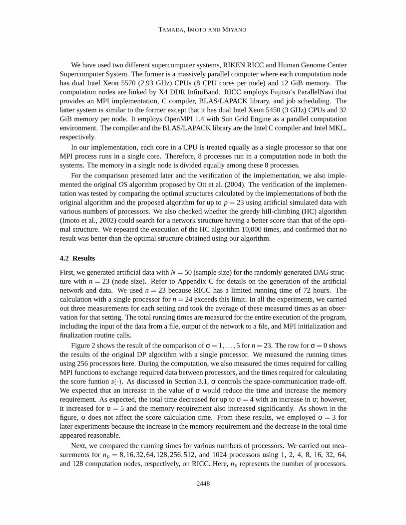
Figure 2 shows the result of the comparison ofσ = 1, . . . ,5 for n= 23. The row forσ = 0 showsthe results of the original DP algorithm with a single processor. We measuredthe running timesusing 256 processors here. During the computation, we also measured thetimes required for callingMPI functions to exchange required data between processors, and thetimes required for calculatingthe score funtions(·). As discussed in Section 3.1,σ controls the space-communication trade-off.We expected that an increase in the value ofσ would reduce the time and increase the memoryrequirement. As expected, the total time decreased for up toσ = 4 with an increase inσ; however,it increased forσ = 5 and the memory requirement also increased significantly. As shown in thefigure, σ does not affect the score calculation time. From these results, we employedσ = 3 forlater experiments because the increase in the memory requirement and the decrease in the total timeappeared reasonable.

Next, we compared the running times for various numbers of processors.We carried out mea-surements fornp = 8,16,32,64,128,256,512, and 1024 processors using 1, 2, 4, 8, 16, 32, 64,and 128 computation nodes, respectively, on RICC. Here,np represents the number of processors.

2448


0

200

400

600

800

1000

1200

1400

1600

1800

1 2 3 4 5

10

50

100T

ime

in

se

co

nd

s

Me

mo

ry u

sa

ge

in

GiB

σ

Total Time (left)Comm Time (left)Score Time (left)

Memory (right)

σ Total Time Cm Time Sc Time Mem0 - - - 1.271 1713.08 909.36 795.61 1.922 1267.98 458.32 794.27 4.753 1072.85 249.06 795.01 15.014 1033.20 196.04 794.75 43.695 1042.21 191.13 797.00 106.91

Figure 2: Running times and memory requirements withσ = 1, . . . ,5 for n= 23 andN = 50 with256 processors. “Total Time” represents the total time required for execution in seconds,“Cm Time” represents the total communication time required for calling MPI functionswithin the total time; “Sc Time,” the time required for score calculation; and “Mem,”thememory requirement in GiB.

1000

10000

100000

8 32 64 128 256 512

64

256

512

Tim

e in

se

co

nd

s (

log

sca

le)

Sp

ee

du

p

Number of processors

Time (left)Speedup (right)

Ideal Speedup (right) np T(np) S(np) E(np) Tc(np) Rc(np)1 203297.04 1.00 1.00 0.00 0.008 26367.58 7.71 0.96 145.24 0.01

16 13563.89 14.99 0.94 490.24 0.0432 6932.09 29.33 0.92 398.29 0.0664 3574.89 56.87 0.89 302.46 0.08

128 1909.72 106.45 0.83 269.90 0.14256 1072.85 189.49 0.74 249.06 0.23512 667.38 304.62 0.59 251.46 0.38

1024 515.29 394.53 0.39 305.12 0.59

Figure 3: Scalability test results forn= 23 andN = 50 with σ = 3. We did not present the resultfor np = 1024 in the graph on the left-hand side because the speedup was too low.

As mentioned above, we usedσ = 3. Fornp = 1, we used the implementation of the original DPalgorithm. Therefore, we do not use the super-combination-based separation of our proposed al-gorithm although it works fornp = 1. Figure 3 shows the experimental result. We evaluated theparallelization scalability of the proposed algorithm from the speedupS(np) and efficiencyE(np).The speedupS(np) is defined asS(np) = T(1)/T(np), wherenp is the number of processors andT(np), the running time withnp processors. IfS(np) = np, then it is called the ideal speedup wherenp-hold speedup is obtained bynp processors. The parallelization efficiencyE(np) is defined asE(np) = S(np)/np. In the case of ideal speedup,E(np) = 1 for anynp. Generally, parallel programs

2449


100

1000

10000

20 21 22 23 24 25 26 27

10

20

30

40

50 60

Tim

e in

se

co

nd

s (

log

sca

le)

Me

mo

ry u

sa

ge

in

GiB

(lo

g s

ca

le)

Number of nodes

Total Time (left)Comm Time (left)Score Time (left)

Memory (right)n Total Cm Time (ratio) Sc Time Mem

20 105.54 31.35 0.30 69.71 5.7721 261.84 66.77 0.26 187.91 8.0022 546.07 188.80 0.35 344.00 10.9723 1072.85 249.06 0.23 795.01 15.0124 2645.04 579.61 0.22 1999.56 20.5525 5386.38 1127.62 0.21 4095.74 28.5026 11976.90 2374.81 0.20 9199.75 40.2527 23686.51 5174.94 0.22 17517.04 59.31

Figure 4: Comparison of running tims for various network sizes. Columnn represents the size ofthe network and “(ratio),” the ratio of “Cm Time” to “Total.” “Mem” is represented inGiB. Other columns have the same meaning as in Figure 2.

that haveE(np)≥ 0.5 are considered to be successfully parallelized. As shown in the table in Fig-ure 3, the efficiencies are 0.74 and 0.59 for np = 256 and 512, respectively. However, with 1024processors, the efficiency became 0.39 and the speedup was very low as compared to that with 512processors, and therefore, it is not efficient and feasible. From these results, we can conclude thatthe program can run very efficiently in parallel for up to 256 processors, and acceptably for up to512 processors.

Tc(np) in Figure 3 represents the time required for calling MPI functions during the executions,andRc(np) is a ratio ofTc(np) to the total timeT(np). Except fornp = 8, Tc(np) decreases withan increase innp because the amount of communication for which each processor is responsibledecreases. However, it did not decrease linearly; in fact, fornp ≥ 512, it increased. This may indi-cate the current limitation of both our algorithm and the computer used to carry out this experiment.For np = 8, Tc(np) was very small. This is mainly because communication between computationnodes was not required for this number of processors. If we subtract Tc(np) from T(np), then theefficiencyE(np) becomes 0.96, 0.95, and 0.94 for 256, 512, and 1024 processors, respectively. Thisresult suggests that the redundant calculation in our proposed algorithmdoes not have a great ef-fect, and the communication cost is the main cause of the inefficiency of our algorithm. Therefore,improving the communication speed in the future may significantly improve the efficiency of thealgorithm with a larger number of processors.

Next, we compared the running times for various network sizes. We generated artificial sim-ulated data forn = 20 to 27 as we did for the above experiment withn = 23. We measured therunning times with 256 processors andσ = 3. Figure 4 shows the result. As shown in the figure,both the time and the space required increased exponentially. Note that both the left- and the right-hand side y-axes are in log scale. The communication time decreased slightly forup ton= 26 withan increase inn. However, forn= 27, it started to increase. From these results, we can say that thescore calculation remains dominant and the communication does not contribute significantly to thetotal running times for this range ofn with np = 256.

2450


0

2000

4000

6000

8000

10000

50 100 150 200 250 300 350 400

Tim

e in

sec

onds

Number of nodes

Total TimeComm TimeScore Time

N Total Cm Time Sc Time50 1072.85 249.06 795.01

100 1775.73 255.55 1492.78150 2490.77 261.01 2201.52200 2863.91 302.04 2533.35250 3684.08 276.14 3379.34300 5460.16 309.71 5122.12350 7354.91 281.40 7045.05400 8698.11 276.68 8392.88

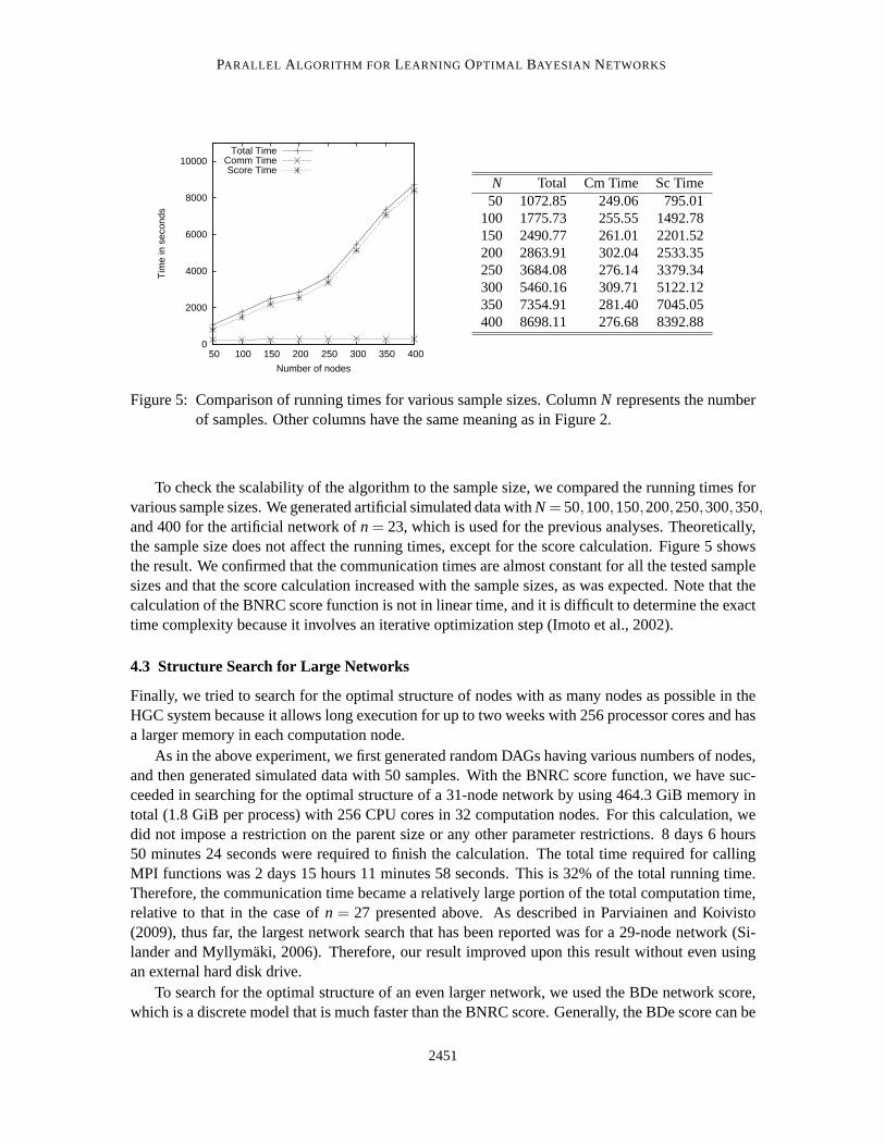
Figure 5: Comparison of running times for various sample sizes. ColumnN represents the numberof samples. Other columns have the same meaning as in Figure 2.

To check the scalability of the algorithm to the sample size, we compared the running times forvarious sample sizes. We generated artificial simulated data withN= 50,100,150,200,250,300,350,and 400 for the artificial network ofn= 23, which is used for the previous analyses. Theoretically,the sample size does not affect the running times, except for the score calculation. Figure 5 showsthe result. We confirmed that the communication times are almost constant for all the tested samplesizes and that the score calculation increased with the sample sizes, as was expected. Note that thecalculation of the BNRC score function is not in linear time, and it is difficult to determine the exacttime complexity because it involves an iterative optimization step (Imoto et al., 2002).

4.3 Structure Search for Large Networks

Finally, we tried to search for the optimal structure of nodes with as many nodes as possible in theHGC system because it allows long execution for up to two weeks with 256 processor cores and hasa larger memory in each computation node.

As in the above experiment, we first generated random DAGs having various numbers of nodes,and then generated simulated data with 50 samples. With the BNRC score function, we have suc-ceeded in searching for the optimal structure of a 31-node network by using 464.3 GiB memory intotal (1.8 GiB per process) with 256 CPU cores in 32 computation nodes. Forthis calculation, wedid not impose a restriction on the parent size or any other parameter restrictions. 8 days 6 hours50 minutes 24 seconds were required to finish the calculation. The total time required for callingMPI functions was 2 days 15 hours 11 minutes 58 seconds. This is 32% of the total running time.Therefore, the communication time became a relatively large portion of the total computation time,relative to that in the case ofn = 27 presented above. As described in Parviainen and Koivisto(2009), thus far, the largest network search that has been reportedwas for a 29-node network (Si-lander and Myllymaki, 2006). Therefore, our result improved upon this result without even usingan external hard disk drive.

To search for the optimal structure of an even larger network, we used the BDe network score,which is a discrete model that is much faster than the BNRC score. Generally,the BDe score can be

2451


calculated 100 times faster than the BNRC score (data not shown). Using theBDe score function,we successfully carried out optimal structure search for a 32-node network without any restrictionusing 836.1 GiB memory (3.3 GiB per process) in total with 256 CPU cores. Thetotal computationtime was 5 days 14 hours 24 minutes and 34 seconds. The MPI communication time was 4 days12 hours 56 minutes 26 seconds, and this is 81% of the total time. Thus, forn = 32 with theBDe score function, the calculation of score functions requires relatively very little time (actually, itrequired only around 1.5 hours per process) as compared to the total time,and the communicationcost becomes the dominant part and the bottleneck of the calculation.

These results show that our algorithm is applicable to the optimal structure search of relativelylarge-sized networks and it can be run on modern low-cost supercomputers.

5. Discussions

In this paper, we have presented a parallel algorithm to search for the score-based optimal structureof Bayesian networks. The main feature of our algorithm is that it can run very efficiently on mas-sively parallel computers in parallel. We confirmed the scalability of the algorithm to the numberof processors through computational experiments and successfully demonstrated optimal structuresearch for a 32-node network with 256 processors, an improvement over the most successful resultreported thus far. Our algorithm overcomes the bottleneck of the previousalgorithm by using alarge amount of distributed memory for large-scale Bayesian network structure search.

Our algorithm has a feature similar to that of an algorithm recently proposed by Parviainen andKoivisto (2009) that requires less space. Both algorithms divide the search space of the problem,and provide a way to compute the optimal structure in parallel. Both are capableof breaking thecurrent limitation of the network size in optimal network structure search. However, these two algo-rithms differ in several respects. First, Parviainen and Koivisto (2009)primarily intended to developa space-time trade-off algorithm to overcome the bottleneck of the search problem. They found thatthe search problem can be divided into sub-problems and that these sub-problems can be solvedindependently with less space. Therefore, although the time requirement increases with a decreasein the space requirement, they mentioned that their algorithm can obtain the optimalstructure for a34-node network by massive parallelization. Our algorithm, on the other hand, overcomes the bot-tleneck in a more straightforward way. We found a way to divide the DP stepsof the fastest knownalgorithm with a relatively low overhead cost. In terms of memory requirement, our algorithm con-sumes much more memory space than that of Parviainen and Koivisto (2009) and even more thanthe original DP algorithm to realize parallelization. However, our algorithm can actually search forthe optimal structure of a 32-node network with 256 processors in less thana week, including scorecalculation, whereas Parviainen and Koivisto (2009) computed only the partial problems. Theirestimate from their empirical result is 4 weeks using 100 processors to obtainthe optimal structurefor a 31-node network. In addition, their estimate ignores the parallelization overhead that generallybecomes problematic in parallelization as well as score calculation, which requires the most time inthe actual application. We showed that our algorithm works efficiently with upto 256 processors,and acceptably with up to 512 processors. An optimal search for even larger networks may be real-ized by improving the current implementation. Our implementation regards each processor core ina CPU equivalently. Therefore, exploiting the modern multi-core CPUs can reduce the communica-tions required among computation nodes and increase the amount of memory space for independentcalculations without requiring improved hardware relative to current supercomputers.

2452


Acknowledgments

Computational time was provided by the Supercomputer System, Human Genome Center, Insti-tute of Medical Science, The University of Tokyo; and RIKEN Supercomputer system, RICC. Thisresearch was supported by a Grant-in-Aid for Research and Development Project of the Next Gen-eration Integrated Simulation of Living Matter at RIKEN and by MEXT, Japan. The authors wouldlike to thank the anonymous referees for their valuable comments.

Appendix A. Definitions of Score Functions

In this paper, we use BNRC (Imoto et al., 2002) and BDe (Heckerman et al.,1995) as a scorefunction s(·) for computational experiments of the proposed algorithm. Here, we present briefdefinitions of these score functions.

A.1 The BNRC Score Function

BNRC is a score function for modeling continuous variables. In a continuousmodel, we considerthe joint density of the variables instead of their joint probability. We search the network structureG by maximizing the posterior ofG for the input data matrixX. The posterior ofG is given by

π(G|X) = π(G)∫ N

∏i=1

n

∏j=1

f (xi j |paGi j ;θ j)π(θG|λ)dθG,

whereπ(G) is the prior distribution ofG; f (xi j |paGi j ;θ j), the local conditional density for thej-th

variable; paGi j = (pa( j)

i1 , . . . , pa( j)iq j), the set of observations in thei-th sample ofq j variables that

represents the direct parents of thej-th node in a network;θG = (θ1, . . . ,θn), the parameter vectorof the conditional densities to be estimated; andπ(θG|λ), the prior distribution ofθG specified bythe hyperparameterλ. Conditional densityf (xi j |paG

i j ;θ j) is modeled by nonparametric regressionwith B-spline basis functions given by

f (xi j |paGi j ;θ j) =

1√

2πσ2j

exp

[

−{xi j −∑q j

k=1mjk(pa( j)ik )}2

2σ2j

]

,

wheremjk(p( j)ik ) = ∑

M jk

l=1 γ( j)lk b( j)

lk (p( j)ik ), {b( j)

1k (·), . . . ,b( j)M jk,k

(·)} is the prescribed set ofM jk B-splines;

σ j , the variance, andγ( j)lk , the coefficient parameters. By taking a−2log of the posterior, the BNRC

score function for thej-th node is defined as

sBNRC(Xj ,PaG(Xj),X) =−2log{

πGj

∫ N

∏i=1

f (xi j |paGi j ;θ j)π j(θ j |λ j)dθ j

}

,

whereπGJ is the prior distribution of the local structure associated with thej-th node; andπ j(θ j |λ j),

the decomposed prior distribution ofθ j specified by the hyperparamterλ j .

2453


A.2 The BDe Score Function

BDe, a score function for the discrete model, can be applied to discrete (categorical) data. As in thecase of BNRC, BDe also considers the posterior ofG; that is,

P(G|X) ∝ P(G)∫

P(X|G,θ)P(θ|G)dθ,

whereP(X|G,θ) is the product of local conditional probabilities (likelihood ofX given G) andP(θ|G), the prior distribution for parametersθ. In the discrete model, we employ multinomialdistribution for modeling the conditional probability and the Dirichlet distribution as its prior dis-tribution. Let Xj be a discrete random variable corresponding to thej-th node, which takes oneof r values{u1, . . . ,ur}, wherer is the number of categories ofXj . In this model, the conditionalprobability ofXj is parameterized as

P(Xj = uk|PaG(Xj) = u jl ) = θ jlk ,

whereu jl (l = 1, . . . , rq j ) is a combination of values for the parents andq j , the number of parents ofthe j-th node. Note that∑r

k=1 θ jlk = 1. For the discrete model, the likelihood can be expressed as

P(X|G,θ) =n

∏j=1

rqj

∏l=1

r

∏k=1

θNjlk

jlk ,

whereNjlk is the number of observations for thej-th node whose values equaluk in the data matrixX with respect to a combination of the parents’ observationl . Njl = ∑r

k=1Njlk andθ denotes a set ofparametersθ jlk . For the parameter setθ, we assume the Dirichlet distribution asπ(θ|G); then, themarginal likelihood can be described as

∫P(X|G,θ)P(θ|G)dθ =

n

∏j=1

rqj

∏l=1

Γ(α jl )

Γ(α jl +Njl )

r

∏k=1

Γ(α jlk +Njlk)

Γ(α jlk),

whereθ is a set of parameters;α jlk , a hyperparameter for the Dirichlet distribution; andα jl =

∑rk=1 α jlk . By taking− log of the posterior, the BDe score function for thej-th node is defined as

sBDe(Xj ,PaG(Xj),X) =− logπGj − log

{

rqj

∏l=1

Γ(α jl )

Γ(α jl +Njl )

r

∏k=1

Γ(α jlk +Njlk)

Γ(α jlk)

}

,

whereπGj is the prior probability of the local structure associated with thej-th node.

Appendix B. Proof of Corollary 10

Proof We prove that(n−σ

k

)

·(k+σ

k

)

=(n

k

)

O(nσ).

(

n−σk

)

·

(

k+σk

)

=(n−σ)!

k!(n−σ−k)!·

(k+σ)!k!(k+σ−k)!

=(n−σ)!

k!(n−σ−k)!·(k+σ)!

k!σ!·(n−k)!(n−k)!

·n!n!

2454


=n!

k!(n−k)!·(n−σ)!(k+σ)!(n−k)!

(n−σ−k)!k!σ!n!

=

(

nk

)

·(n−σ)!

(n−σ−k)!·(k+σ)!

k!σ!·(n−k)!

n!

=

(

nk

)

·(n−σ)

n(n−σ−1)(n−1)

· · ·(n−σ−k+1)(n−k+1)

·(k+σ) · · ·(k+1)k!

σ!k!

=

(

nk

)

·O(1) ·O((k+σ)σ) =

(

nk

)

·O((k+σ)σ).

For n < k+σ, we consider only super-combinations of sizen. Thus, for eachk, there are atmost

(nk

)

O(nσ) calculations.

Appendix C. Method for Generating Artificial Network and Data

To generate the random DAG structure, we simply added edges at randomto an empty graph sothat the acyclic structure is maintained and the average degree becomesd = 4.0. Consequently, thenumber of total edges equalsn ·d/2. Note that the degree of DAGs does not affect the executiontime of the algorithm as the algorithm searches all possible structures. To generate the artificial data,we first randomly assigned 8 different nonlinear or linear equations to theedges and then generatedthe artificial numerical values based on the normal distribution and the assigned equations. Figure 6shows the assigned equations and examples of the generated data. If a node has more than twoparent nodes, the generated values are summed before adding the noise. We set the noise ratio to be0.2.

To apply BDe to the artificial data on then = 32 network, we discretized the continuous datagenerated by the same method for all variables into three categories (r = 3) and then executed thealgorithm for these discretized values.

Appendix D. Efficient Indexing of Combinations

When running the algorithm, we need to generate combination vectors discontinuously and indepen-dently in a processor. To do this efficiently, we require an algorithm that calculates a combinationvector from its index and the index from its combination vector. Buckles and Lybanon (1977) pre-sented an efficient lexicographical index - vector conversion algorithm.However, this algorithmrequires the calculation of binomial coefficients for every possible elementin a combination everytime. To speed up this calculation, we developed a linear time algorithm that needed polynomialtime to construct a reusable table (Tamada et al., 2011). Our algorithm actuallydeals withthe re-verse lexicographical indexinstead of the ordinal lexicographical index; this enables us to calculatethe table only once and to make it reusable. In this section, we present the algorithms as describedin Tamada et al. (2011). See Tamada et al. (2011) for details and the proofs of the theorems. In thissection, note that we assume that∑n

i=k fi = 0 for any fi if n< k.

Theorem 13 (RLI calculation) Let C = {C1,C2, . . . ,Cm} be the set of all the combinations oflength k taken from n objects, arranged in lexicographical order, wherem=

(nk

)

. We call i the lex-icographical index of Ci ∈ C . Let us define the reverse lexicographical index of Ci ∈ C , RLI(Ci ,n)

2455


(a) fa(X) = X+ ε

(b) fb(X) =−X+ ε

(c) fc(X) = 11+e−4X + ε

(d) fd(X) =− 11+e−4X + ε

(e) fe(X) =−(X−1.5)2+ ε

(f) f f (X) = (−X−2.5)2+ ε

(g) fg(X) =−(−X−2.5)2+ ε

(h) fh(X) = (X−1.5)2+ ε

−4 0 2

−2

02

4

−2 2 6

−4

02

4

−2 0 1 2

−4

−2

02

−6 −2 2 4

−3

−1

13

−4 0 2 4

−4

02

4

−6 −2 2 4

−2

02

4

−2 0 1 2

−4

02

4

−4 0 2 4 6

−4

02

4

(a)

(b)

(c)

(d)

(e)

(f)

(g)

(h)

Figure 6: Left: Linear and nonlinear equations assigned to each edge in artificial networks.ε repre-sents the noise based on the normal distribution. Right: Examples of the valuesgeneratedby these equations.

1,2,3

1,2,4

1,2,5

1,2,6

1,3,4

1,3,5

1,3,6

1,4,5

1,4,6

1,5,6

2,3,4

2,3,5

2,3,6

2,4,5

2,4,6

3,4,5

3,4,6

3,5,6

4,5,6

2,5,6

1

2

3

4

5

6

7

8

9

10

11

12

13

14

15

16

17

18

19

20

RLI(X, n) X

5

2( )

4

2( )

3

2( )

= 10

= 6

= 3

2

2( ) = 1

4

2( ) 3

2( ) 2

2( )+ + = 5

3( ) = 10

3

2( ) = 4

3( ) = 42

2( )+

4

1( )

3

1( )2

1( )1

1( )

3

1( ) 2

1( ) 1

1( )+ + = 4

2( ) = 6

2

1( ) 1

1( )+ = 3

2( ) = 3

Figure 7: RLI calculation forn= 6 andk= 3.

def= m− i +1. Suppose that we consider a combination of natural numbers, that is, some combina-tion X = {x1,x2, . . . ,xk} ∈ C , where xi < x j if i < j and xi ∈ {1,2, . . . ,n}. Then, RLI(X,n) can be

2456


Algorithm 3 RLITable(m) generates the index table for conversion between a combination and theindex.Input: m: maximum number of elements appearing in a combination,Output: T : m×m index table.

1: {Initialization}2: T(i,1)← 0 (1≤ i ≤m).3: T(1, j)← j−1 (2≤ j ≤m).4: {Main Routine}5: for i = 2 tomdo6: for j = 2 tomdo7: T(i, j)← T(i−1, j)+T(i, j−1).8: end for9: end for

10: return T.

Algorithm 4 RLI(X,n,T) calculates the reverse lexicographical index of the given combinationX.

Input: X = {x1,x2, . . .xk} (x1 < · · ·< xk ∧ 1≤ xi ≤ n) : input combination of lengthk taken fromn objects,n: total number of elements,T : index table calculated byRLITable(·).

Output: reverse lexicographical index of combinationX.1: r ← 02: for i = 1 tok do3: r ← z+T(k− i+1,n−k−xi + i+1).4: end for5: return r +1.

calculated by

RLI(X,n) =|X|

∑i=1

(

n−xi

|X|− i+1

)

+1.

Figure 7 shows an example of the calculation of RLI forn = 6 andk = 3. For example,RLI({1,3,5},6) =

(53

)

+(3

2

)

+(1

1

)

+1= 15.

Corollary 14 (RLI calculation by the index table) Let T be a(k,n−k+1)-size matrix whose ele-

ment T(α,β) def=

(α+β−2α

)

. Matrix T can be calculated only by(n−1)(n−k−1) time addition and byusing T , RLI(X,n) can be calculated in linear time by RLI(X,n)=∑k

i=1T(k− i+1,n−k−xi+ i+1)+ 1.

Algorithm 3 shows the pseudocode used to generateT and Algorithm 4, the pseudocode ofRLI(X,n). The inverse function that generates the combination vector for an RLI can be calculatedby simply finding the largest column position ofT, subtracting the value in the table from the index,and then repeating thisk times.

Corollary 15 Let RLI(X,n) be the reverse lexicographical index defined above for combination X= {x1,x2, . . . ,xk}. The inverse function of RLI(X,n), that is, the i-th element xi of

2457


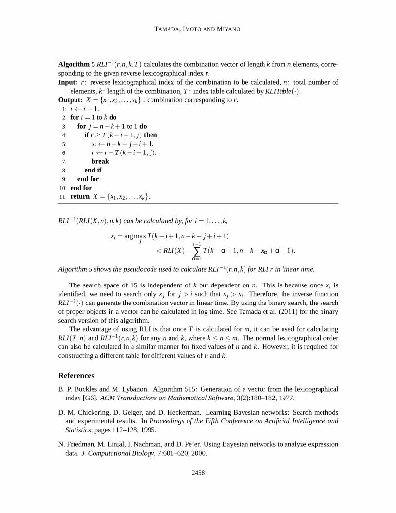
Algorithm 5 RLI−1(r,n,k,T) calculates the combination vector of lengthk from n elements, corre-sponding to the given reverse lexicographical indexr.Input: r : reverse lexicographical index of the combination to be calculated,n: total number of

elements,k: length of the combination,T : index table calculated byRLITable(·).Output: X = {x1,x2, . . . ,xk} : combination corresponding tor.

1: r ← r−1.2: for i = 1 tok do3: for j = n−k+1 to 1do4: if r ≥ T(k− i+1, j) then5: xi ← n−k− j + i+1.6: r ← r−T(k− i+1, j).7: break8: end if9: end for

10: end for11: return X = {x1,x2, . . . ,xk}.

RLI−1(RLI(X,n),n,k) can be calculated by, for i= 1, . . . ,k,

xi = argmaxj

T(k− i+1,n−k− j + i+1)

< RLI(X)−i−1

∑α=1

T(k−α+1,n−k−xα +α+1).

Algorithm 5 shows the pseudocode used to calculate RLI−1(r,n,k) for RLI r in linear time.

The search space of 15 is independent ofk but dependent onn. This is because oncexi isidentified, we need to search onlyx j for j > i such thatx j > xi . Therefore, the inverse functionRLI−1(·) can generate the combination vector in linear time. By using the binary search,the searchof proper objects in a vector can be calculated in log time. See Tamada et al. (2011) for the binarysearch version of this algorithm.

The advantage of using RLI is that onceT is calculated form, it can be used for calculatingRLI(X,n) andRLI−1(r,n,k) for anyn andk, wherek≤ n≤ m. The normal lexicographical ordercan also be calculated in a similar manner for fixed values ofn andk. However, it is required forconstructing a different table for different values ofn andk.

References

B. P. Buckles and M. Lybanon. Algorithm 515: Generation of a vector from the lexicographicalindex [G6]. ACM Transductions on Mathematical Software, 3(2):180–182, 1977.

D. M. Chickering, D. Geiger, and D. Heckerman. Learning Bayesian networks: Search methodsand experimental results. InProceedings of the Fifth Conference on Artificial Intelligence andStatistics, pages 112–128, 1995.

N. Friedman, M. Linial, I. Nachman, and D. Pe’er. Using Bayesian networks to analyze expressiondata.J. Computational Biology, 7:601–620, 2000.

2458


D. Heckerman, D. Geiger, and D. M. Chickering. Learning Bayesian networks: the combination ofknowledge and statistical data.Machine Learning, 20:197–243, 1995.

S. Imoto, T. Goto, and S. Miyano. Estimation of genetic networks and functional structures be-tween genes by using Bayesian networks and nonparametric regression. Pacific Symposium onBiocomputing, 7:175–186, 2002.

M. Koivisto and K. Sood. Exact Bayesian structure discovery in Bayesian networks.Journal ofMachine Learning Research, 5:549–573, 2004.

S. Ott, S. Imoto, and S. Miyano. Finding optimal models for small gene networks. Pacific Sympo-sium on Biocomputing, 9:557–567, 2004.

P. Parviainen and M. Koivisto. Exact structure discovery in Bayesian networks with less space.Proceedings of the 25th Conference on Uncertainty in Artificial Intelligence(UAI 2009), 2009.

J. Pearl.Probabilistic Reasoning in Intelligent Systems: Networks of Plausible Inference. MorganKaufman Publishers, San Mateo, CA, 1988.

E. Perrier, S. Imoto, and S. Miyano. Finding optimal Bayesian network given a super-structure.J.Machine Learning Research, 9:2251–2286, 2008.

T. Silander and P. Myllymaki. A simple approach for finding the globally optimal Bayesian networkstructure. Proceedings of the 22th Conference on Uncertainty in Artificial Intelligence(UAI2006), pages 445–452, 2006.

Y. Tamada, S. Imoto, and S. Miyano. Conversion between a combination vector and the lexico-graphical index in linear time with polynomial time preprocessing, 2011.submitted.

I. Tsamardinos, L. E. Brown, and C. F. Aliferis. The max-min hill-climbing Bayesian networkstructure learning algorithm.Machine Learning, 65:31–78, 2006.

2459

parallel algorithm for learning optimal bayesian...

Documents