P A R TO N E

CHAPTER 2Atomic Bonding

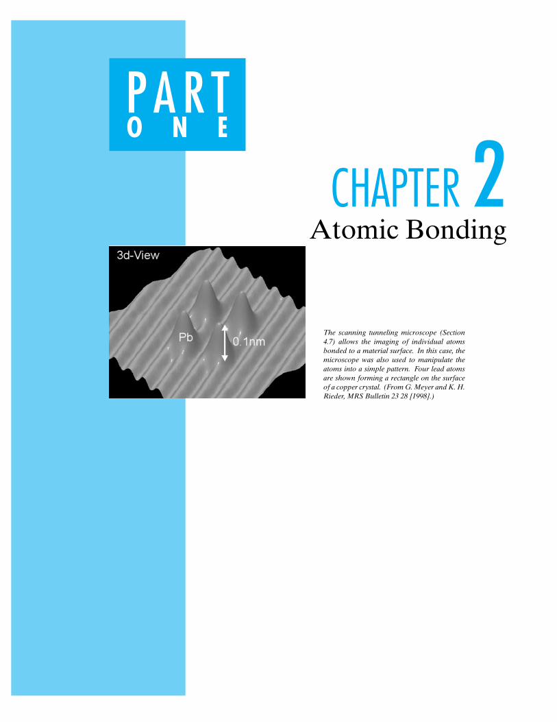
The scanning tunneling microscope (Section4.7) allows the imaging of individual atomsbonded to a material surface. In this case, themicroscope was also used to manipulate theatoms into a simple pattern. Four lead atomsare shown forming a rectangle on the surfaceof a copper crystal. (From G. Meyer and K. H.Rieder, MRS Bulletin 23 28 [1998].)

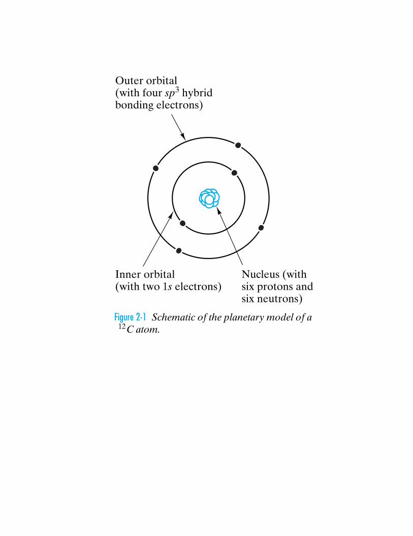
Outer orbital(with four sp3 hybridbonding electrons)

Nucleus (withsix protons andsix neutrons)

Inner orbital(with two 1s electrons)

Figure 2-1 Schematic of the planetary model of a12C atom.

1H

1.008

3Li

6.941

4Be

9.012

I A

II A III A IV A V A VI A VII A

VIII

III B IV B V B VI B VII B I B

11Na

22.99

12Mg

24.31

13Al

26.98

14Si

28.09

15P

30.97

16S

32.06

17Cl

35.45

18Ar

39.95

5B

10.81

6C

12.01

7N

14.01

8O

16.00

9F

19.00

10Ne

20.18

2He

4.003

0

19K

39.10

20Ca

40.08

21Sc

44.96

22Ti

47.90

23V

50.94

24Cr

52.00

25Mn

54.94

26Fe

55.85

27Co

58.93

28Ni

58.71

29Cu

63.55

30Zn

65.38

31Ga

69.72

32Ge

72.59

33As

74.92

34Se

78.96

35Br

79.90

36Kr

83.8037Rb

85.47

38Sr

87.62

39Y

88.91

40Zr

91.22

41Nb

92.91

42Mo

95.94

43Tc

98.91

44Ru

101.07

45Rh

102.91

46Pd

106.4

47Ag

107.87

48Cd

112.4

49In

114.82

50Sn

118.69

51Sb

121.75

52Te

127.60

53I

126.90

54Xe

131.3055Cs

132.91

56Ba

137.33

57La

138.9187Fr

(223)

88Ra

226.03

89Ac

(227)

72Hf

178.49

73Ta

180.95

74W

183.85

75Re

186.2

76Os

190.2

77Ir

192.22

78Pt

195.09

79Au

196.97

80Hg

200.59

81Tl

204.37

82Pb

207.2

83Bi

208.98

84Po

(210)

58Ce

140.12

59Pr

140.91

60Nd

144.24

61Pm

(145)

62Sm

150.4

63Eu

151.96

64Gd

157.25

65Tb

158.93

66Dy

162.50

67Ho

164.93

68Er

167.26

69Tm

168.93

70Yb

173.04

71Lu

174.9790Th

232.04

91Pa

231.04

92U

238.03

93Np

237.05

94Pu

(244)

95Am

(243)

96Cm

(247)

97Bk

(247)

98Cf

(251)

99Es

(254)

100Fm

(257)

101Md

(258)

102No

(259)

103Lw

(260)

85At

(210)

86Rn

(222)

II B

Figure 2-2 Periodic table of the elements indicating atomic number and atomic mass (in amu).

Energy (eV)

–283.9

–6.52 (sp3)

1s

0

Figure 2-3 Energy-level diagram for the orbital electrons in a 12C atom.Notice the sign convention. An attractive energy is negative. The 1s elec-trons are closer to the nucleus (see Figure 2–1) and more strongly bound(binding energy = −283.9 eV). The outer orbital electrons have a bind-ing energy of only −6.5 eV. The zero level of binding energy correspondsto an electron completely removed from the attractive potential of thenucleus.

Electron transfer

Ionic bond

Na Cl

Na+ Cl–

Figure 2-4 Ionic bonding between sodiumand chlorine atoms. Electron transfer fromNa to Cl creates a cation (Na+) and ananion (Cl−). The ionic bond is due to thecoulombic attraction between the ions ofopposite charge.

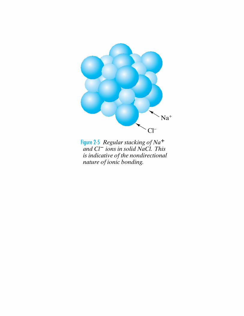
Cl–

Na+

Figure 2-5 Regular stacking of Na+and Cl− ions in solid NaCl. Thisis indicative of the nondirectionalnature of ionic bonding.

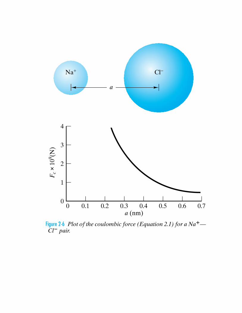
0.70.60.50.40.3a (nm)

Na+ Cl–

0.20.1

a

4

3

2

1

00

Fc

× 10

9 (N)

Figure 2-6 Plot of the coulombic force (Equation 2.1) for a Na+—Cl− pair.

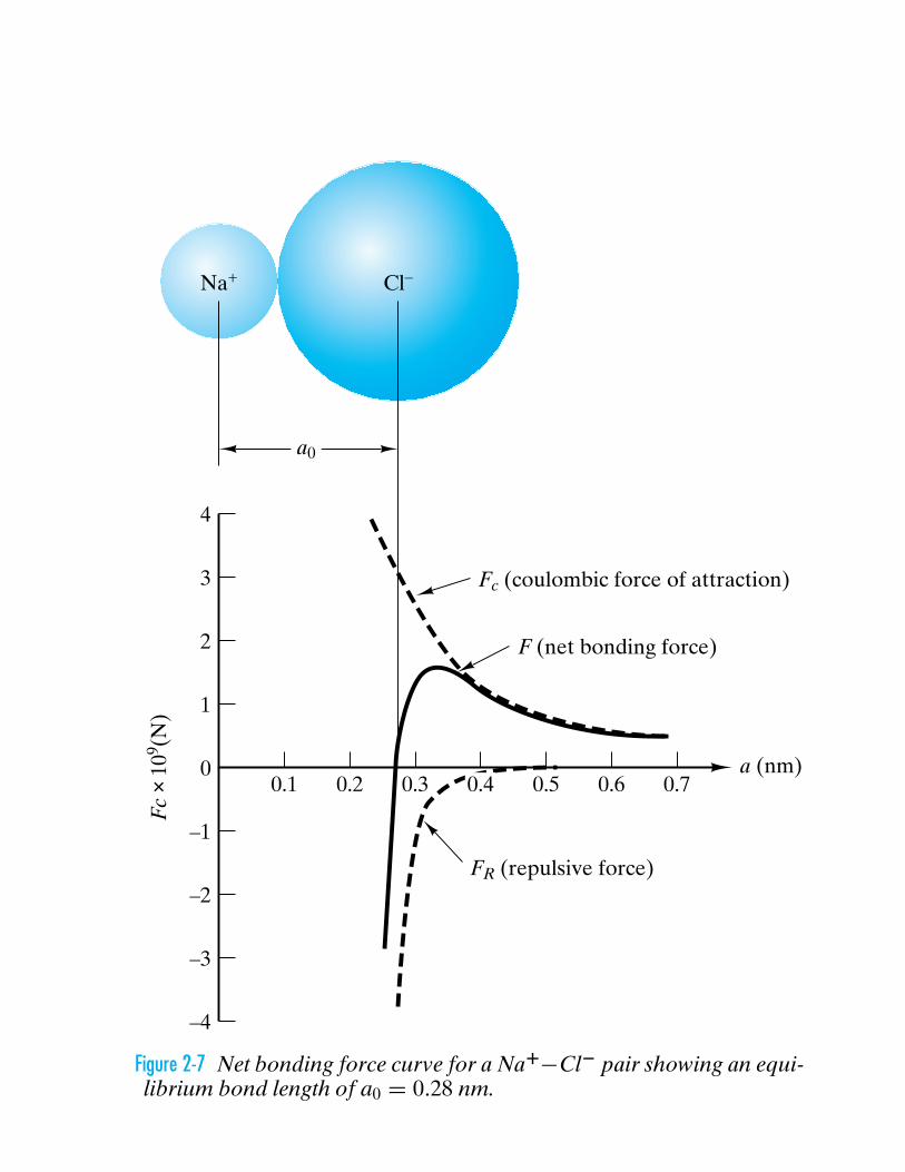
0.7a (nm)

0.60.50.40.3

Na+

Fc (coulombic force of attraction)

FR (repulsive force)

F (net bonding force)

Cl–

0.20.1

a0

4

3

2

1

–1

–2

–3

–4

0

Fc

× 10

9 (N)

Figure 2-7 Net bonding force curve for a Na+−Cl− pair showing an equi-librium bond length of a0 = 0.28 nm.

+

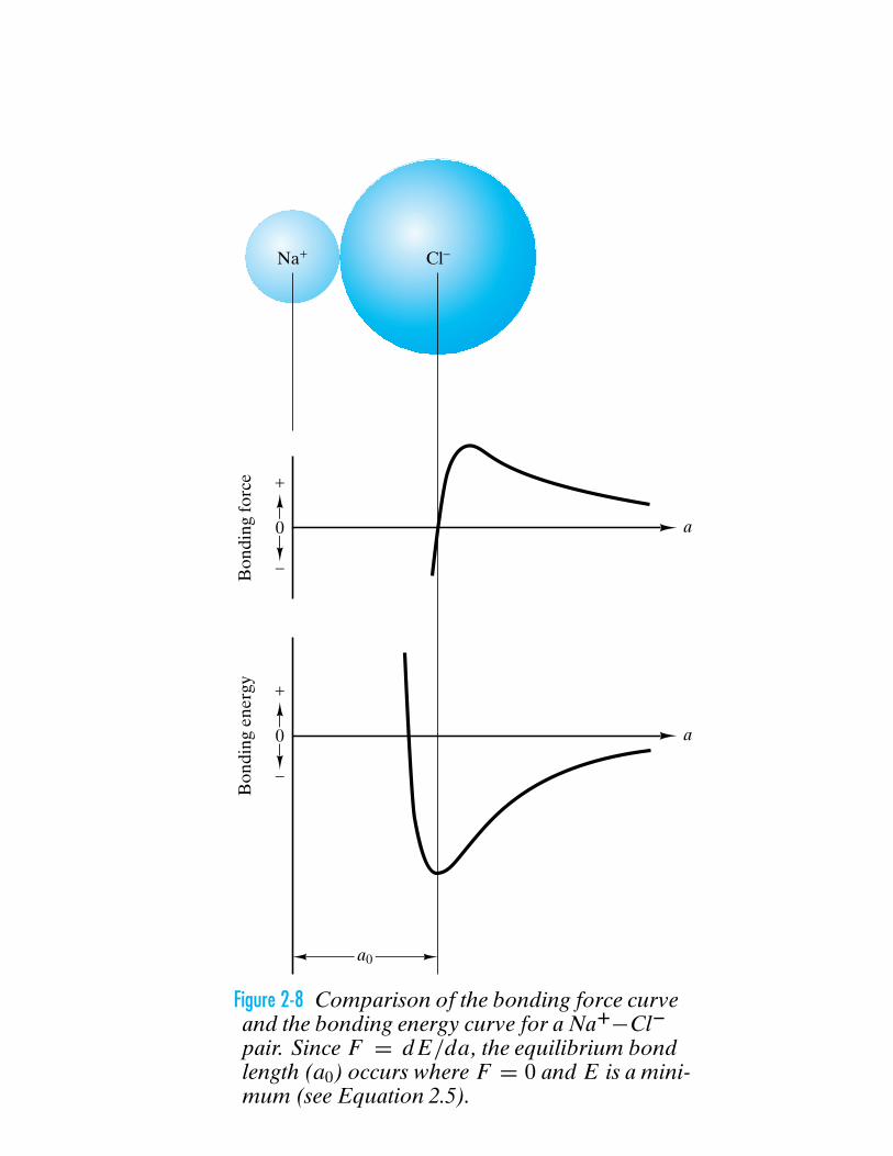
0

–Bon

ding

forc

eNa+ Cl–

a

+

0

a0

–

Bon

ding

ene

rgy

a

Figure 2-8 Comparison of the bonding force curveand the bonding energy curve for a Na+−Cl−pair. Since F = dE/da , the equilibrium bondlength (a0) occurs where F = 0 and E is a mini-mum (see Equation 2.5).

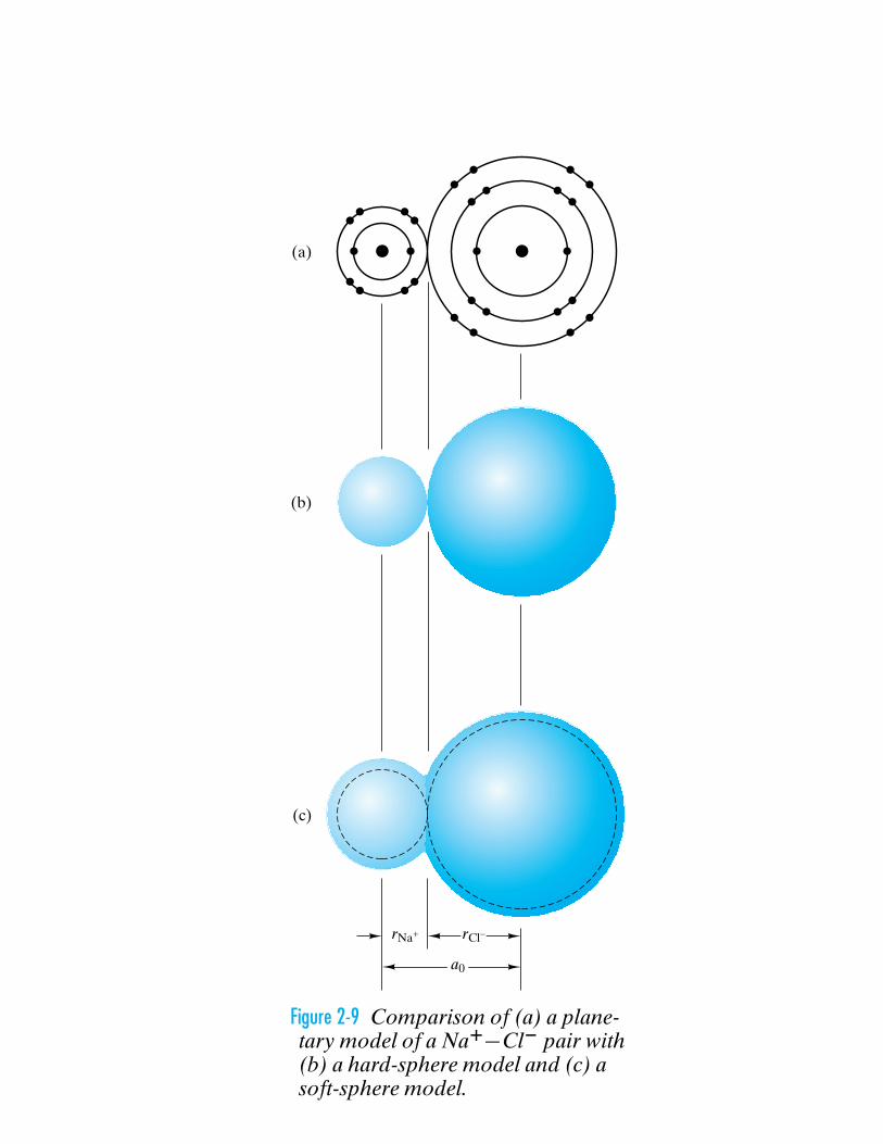
(a)

(b)

(c)

a0

rCl–rNa+

Figure 2-9 Comparison of (a) a plane-tary model of a Na+−Cl− pair with(b) a hard-sphere model and (c) asoft-sphere model.

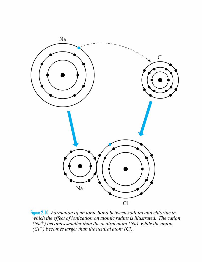
Na

Na+

Cl

Cl–

Figure 2-10 Formation of an ionic bond between sodium and chlorine inwhich the effect of ionization on atomic radius is illustrated. The cation(Na+) becomes smaller than the neutral atom (Na), while the anion(Cl−) becomes larger than the neutral atom (Cl).

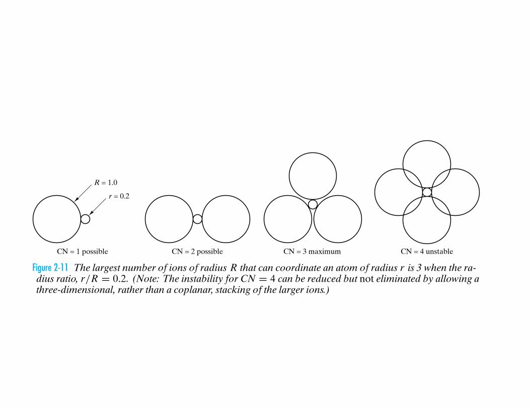
R = 1.0

r = 0.2

CN = 1 possible CN = 2 possible CN = 3 maximum CN = 4 unstable

Figure 2-11 The largest number of ions of radius R that can coordinate an atom of radius r is 3 when the ra-dius ratio, r/R = 0.2. (Note: The instability for CN = 4 can be reduced but not eliminated by allowing athree-dimensional, rather than a coplanar, stacking of the larger ions.)

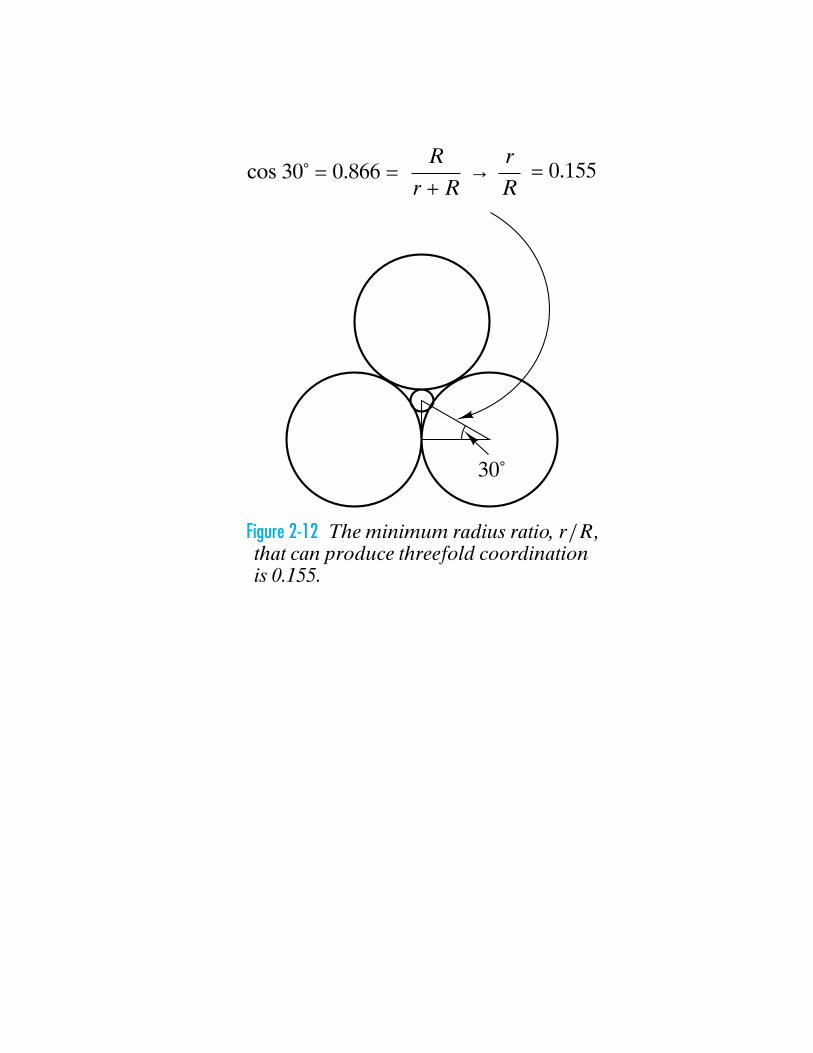
30˚

cos 30˚ = 0.866 = = 0.155R

r + R

r

R→

Figure 2-12 The minimum radius ratio, r/R ,that can produce threefold coordinationis 0.155.

(a)

(b)

(d)

(c)

Cl Cl

Cl Cl

Figure 2-13 The covalent bond ina molecule of chlorine gas, Cl2,is illustrated with (a) a plane-tary model compared with (b)the actual electron density and(c) an “electron-dot” schematicand (d) a “bond-line” schematic.

C C

HH

C C C C C

HH

H H

H H

H

H

H

H

H

H

C C C

H

H

H

H

H

H

(a)

(b)

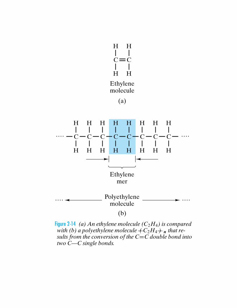
Ethylenemolecule

Ethylenemer

Polyethylenemolecule

. . . .. . . .

. . . .. . . .

Figure 2-14 (a) An ethylene molecule (C2H4) is comparedwith (b) a polyethylene molecule ( C2H4 ) n that re-sults from the conversion of the C=C double bond intotwo C—C single bonds.

C

H

H

C

H

H

CH

H

CH H

CH

HC

H

H

C

H

H

C

H

H

C

H

HC

H

HC HH

C HH

C

H

H

C

H

H

CH

H C

H

H

C

H

H

C

H

HC

H

HC

H

H

C

H

H

C

H

H

CH

H

CHH

CH H

CH H

CHH

CH H

CH H

CH H

CH H

CHH

CH

HC

H

H

C

H

H

C

H

H

C

H

H

C

H

HC

H

H

C

H

HC

H

HC

H

H

C

H

H

C

H

H

C

H

H

C

H

H

C

H

H

C

H

H

C

H

H

CH H

CHH

CH

H

CHH

CH

H

C

H

H

C

H

H

CH

H

CH

H

C

H

H

C

H

H

CH

H

CH

H

CH

H

... .

....

. . . .

.. . .

. . . .

. . . .

. . ..

. . . .

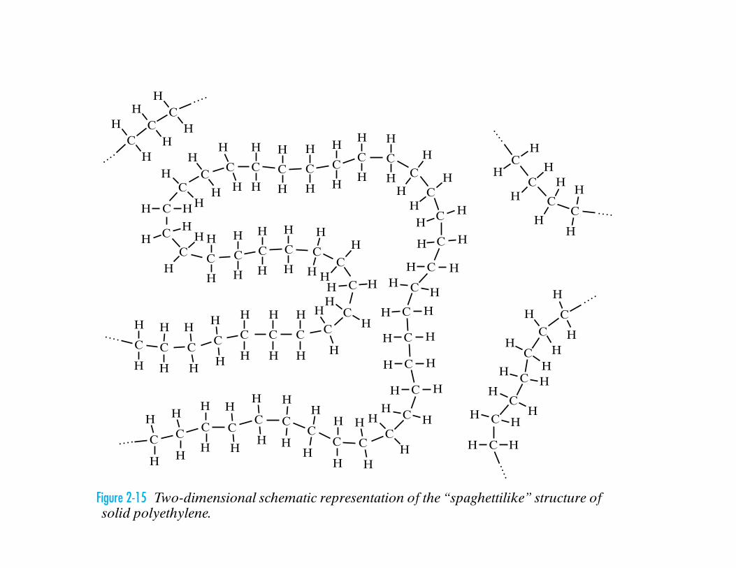
Figure 2-15 Two-dimensional schematic representation of the “spaghettilike” structure ofsolid polyethylene.

C

C C

C C

CC

C

C

CC

C

C

C

C

C

Figure 2-16 Three-dimensional structure of bond-ing in the covalent solid, carbon (diamond).Each carbon atom (C) has four covalent bondsto four other carbon atoms. (This geometry canbe compared with the “diamond cubic” struc-ture of Figure 3–23.) In this illustration, the “bond-line” schematic of covalent bonding is givena perspective view to emphasize the spatial ar-rangement of bonded carbon atoms.

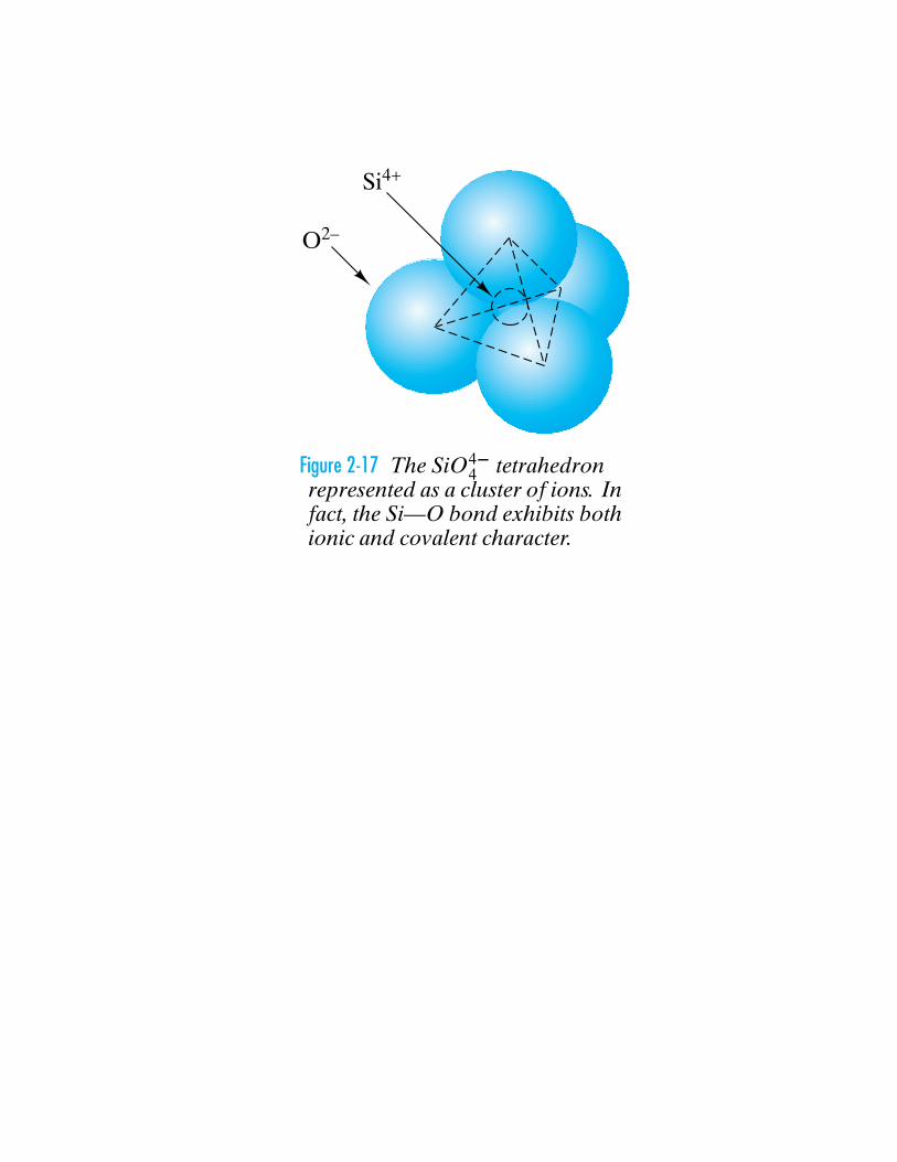
O2–

Si4+

Figure 2-17 The SiO4−4 tetrahedron

represented as a cluster of ions. Infact, the Si—O bond exhibits bothionic and covalent character.

Bond energy

0

+

–

E a

Bond length

Figure 2-18 The general shape of the bond energy curve as well asassociated terminology applies to covalent as well as ionic bond-ing. (The same is true of metallic and secondary bonding.)

109.5˚

C

Figure 2-19 Tetrahedral configuration of covalentbonds with carbon. The bond angle is 109.5◦.

C C

ClH

H H

…… C C C C C

HCl

H H

Cl

H

H

H

C C

Cl

H

H

H

Cl

H

C C C

H

H

Cl

H

H

H

mer

…

…

CC C

C

C

C C C

54.75˚

l109.5˚

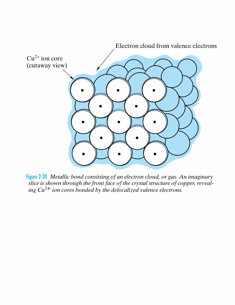
Cu2+ ion core(cutaway view)

Electron cloud from valence electrons

Figure 2-20 Metallic bond consisting of an electron cloud, or gas. An imaginaryslice is shown through the front face of the crystal structure of copper, reveal-ing Cu2+ ion cores bonded by the delocalized valence electrons.

1H2.1

3Li1.0

4Be1.5

I A

II A III A IV A V A VI A VII A

VIII

III B IV B V B VI B VII B I B

11Na0.9

12Mg1.2

13Al1.5

14Si1.8

15P

2.1

16S

2.5

17Cl3.0

18Ar–

5B

2.0

6C

2.5

7N3.0

8O3.5

9F

4.0

10Ne–

2He–

0

19K0.8

20Ca1.0

21Sc1.3

22Ti1.5

23V1.6

24Cr1.6

25Mn1.5

26Fe1.8

27Co1.8

28Ni1.8

29Cu1.9

30Zn1.6

31Ga1.6

32Ge1.8

33As2.0

34Se2.4

35Br2.8

36Kr–

37Rb0.8

38Sr1.0

39Y1.2

40Zr1.4

41Nb1.6

42Mo1.8

43Tc1.9

44Ru2.2

45Rh2.2

46Pd2.2

47Ag1.9

48Cd1.7

49In1.7

50Sn1.8

51Sb1.9

52Te2.1

53I

2.5

54Xe–

55Cs0.7

56Ba0.9

57-71La-Lu1.1-1.2

87Fr0.7

88Ra0.9

89-102Ac-No1.1-1.7

72Hf1.3

73Ta1.5

74W1.7

75Re1.9

76Os2.2

77Ir2.2

78Pt2.2

79Au2.4

80Hg1.9

81Tl1.8

82Pb1.8

83Bi1.9

84Po2.0

85At2.2

86Rn–

II B

Figure 2-21 The electronegativities of the elements. (After Linus Pauling, The Nature of the Chemical Bondand the Structure of Molecules and Crystals; An Introduction to Modern Structural Chemistry, 3rd ed.,Cornell University Press, Ithaca, New York, 1960)

+–

Magnitude ofdipole moment

Secondarybond

Isolated Ar atom

+–

Isolated Ar atom

Center of negative(electron) charge

Center of positivecharge (nucleus)

Figure 2-22 Development of induced dipoles in adjacent argon atoms leading to a weak, secondary bond. The de-gree of charge distortion shown here is greatly exaggerated.

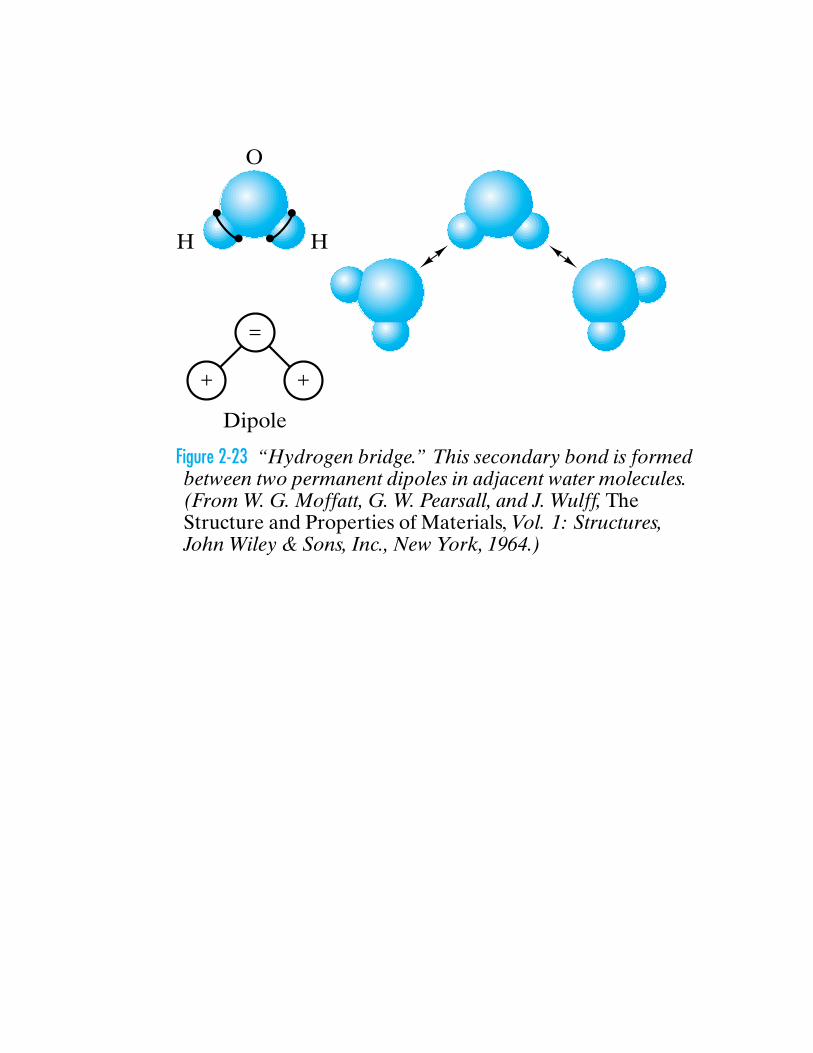
Dipole

HH

O

+

=

+

Figure 2-23 “Hydrogen bridge.” This secondary bond is formedbetween two permanent dipoles in adjacent water molecules.(From W. G. Moffatt, G. W. Pearsall, and J. Wulff, TheStructure and Properties of Materials, Vol. 1: Structures,John Wiley & Sons, Inc., New York, 1964.)

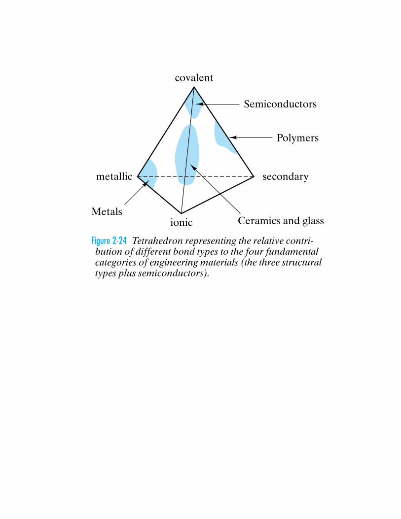
covalent

Semiconductors

Polymers

metallic secondary

Ceramics and glassMetals

ionic

Figure 2-24 Tetrahedron representing the relative contri-bution of different bond types to the four fundamentalcategories of engineering materials (the three structuraltypes plus semiconductors).

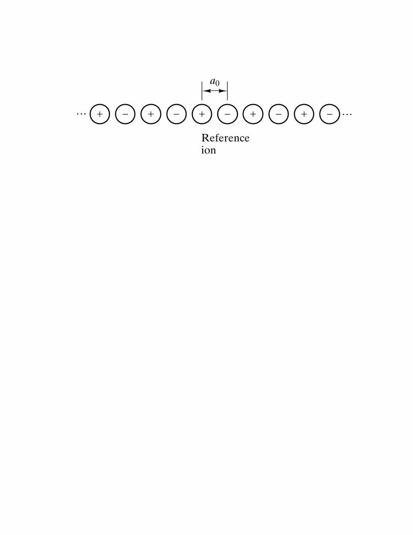
a0

Referenceion

… + – + – + – + – + – …

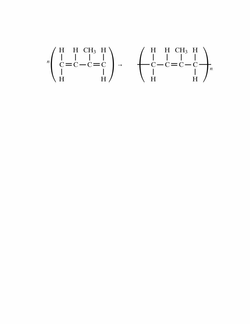
C C

H

C

H

n

n

H H

C

CH3 H

C C

H

C

H

H H

C

CH3 H

→1 2 1 2

n

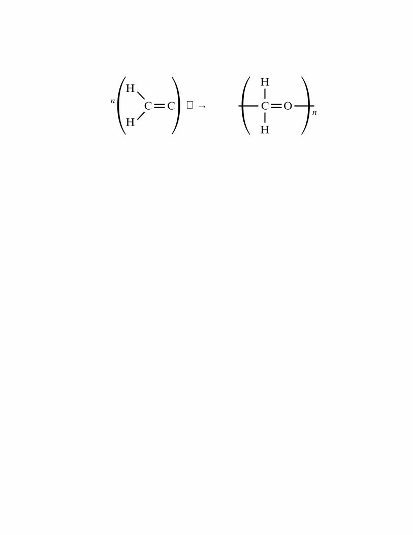
nOC

H

H

CC

H

H

→1 2 1 2

C C

FF

F F

C C

HF

F H

C C

F

F F

C FF

F

Na (solid) + Cl2 (g)

NaCl (solid) Na+ (g) + Cl– (g)

Na (g) + Cl (g)1

2

DHf̊

→

→

→

→

←