Partially Awakened Giants:Uneven Growth in China and India

Martin RavallionWorld Bank

This presentation is based on:• Shubham Chaudhuri and Martin Ravallion,“Partially Awakened Giants: Uneven Growth in

China and India” in Dancing with Giants: China, India, and the Global Economy (edited by L. Alan Winters and Shahid Yusuf), World Bank, 2007.

• Martin Ravallion and Shaohua Chen, “China’s (Uneven) Progress Against Poverty,” Journal of Development Economics, Vol. 82(1), Jan. 2007, pp.1-42.

• Gaurav Datt and Martin Ravallion, “Has India’s Post-Reform Economic Growth Left the Poor Behind,”, Journal of Economic Perspectives Vol. 16(3), Summer 2002, pp. 89-108.

Seminar at Chinese Academy of Social Sciences, Beijing, October 2007

China and India: Growth with poverty reduction, but rising inequality

• Economic growth in China and India since the 1980s has been accompanied by a falling incidence of absolute poverty. =>

• However, concerns are being expressed about the distributional impacts of the growth processes in both countries.

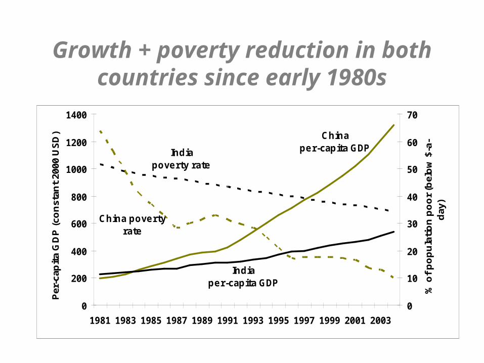
Growth + poverty reduction in both countries since early 1980s

China per-capita GDP

India per-capita GDP

China poverty rate

Indiapoverty rate

0

200

400

600

800

1000

1200

1400

1981 1983 1985 1987 1989 1991 1993 1995 1997 1999 2001 2003

Per

-cap

ita

GD

P (

con

stan

t 20

00 U

SD

)

0

10

20

30

40

50

60

70

% o

f p

op

ula

tio

n p

oo

r (b

elo

w $

-a-

day

)

Signs of rising “income” inequality, although the trend is only clear for China

China (income)

India (consumption)

25.0

30.0

35.0

40.0

45.0

1978 1983 1988 1993 1998 2003

Gin

i co

effi

cien

t o

f in

equ

alit

y

New trend? Too early to say

Long-term trend, though not monotonic

Incidence of growth in the 1990s

0

1

2

3

4

5

6

7

8

9

10

0 10 20 30 40 50 60 70 80 90

The poorest p% of population ranked by per capita income/expenditure

An

nu

al

gro

wth

in

in

co

me

/ex

pe

nd

itu

re p

er

pe

rso

n (

%)

Median

China (income) 1993-2004

India (expenditure)1993/1994-2004/2005

Growth incidence curves for China and India

Aside: Growth incidence curve

Further reading: On the growth incidence curve see Martin Ravallion and Shaohua Chen, “Measuring Pro-Poor Growth”, Economics Letters, 2003.

)(

)()()(

1

1

py

pypypg

t

ttt

where yt(p) is the quantile function: yt=Ft-1(p)

1

( )( ) 1 ( 1)

( )t

t tt

L pg p g

L p

Ordinary growth factor

Distributioncorrection

Growth factor at percentile p

Data issues: China

• Separate urban and rural surveys; comparability problems

• Comparability problems over time, esp., changes in valuation methods in rural household surveys in 1990 (Chen-Ravallion corrections).

• Problems with price deflators (esp., spatial) 

• “Floating population”: Sample frame (pre-2002) based on registrations not street addresses.– Bias due to this is very small

– For example, if 5.0% of urban population is deemed poor, this only falls to 4.6% if one excludes those with rural registration.

Data issues: India

• Highly comparable surveys up to 1999/2000

• Changes in survey design in 1999/2000 have created comparability problems.

• Various corrections (Deaton-Tarozzi; Sundaram-Tendulkar)

• New survey (2004/05) is comparable with 1993/94.

Measurement: What weight on between-group inequalities?

• We focus on aggregate inequality and its sources.

• However, specific between-group inequalities matter more to perceptions of social justice than is evident in standard decompositions

• Urban-rural and geographic inequalities appear to be examples.– China: Salience of regions (coastal-inland) and urban-rural

disparities

– India: “Shining India”? Not if large segments of the rural population are left behind.

How uneven is the growth process?

What does this mean for poverty and inequality?

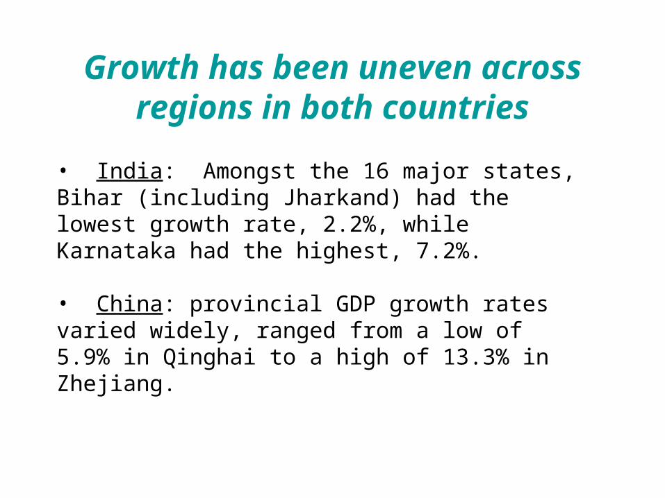
Growth has been uneven across regions in both countries

• India: Amongst the 16 major states, Bihar (including Jharkand) had the lowest growth rate, 2.2%, while Karnataka had the highest, 7.2%. • China: provincial GDP growth rates varied widely, ranged from a low of 5.9% in Qinghai to a high of 13.3% in Zhejiang.

Growth divergence?“Yes” in India, but qualified “no” for China

(though divergence between coastal areas and inland)

0.0

2.0

4.0

6.0

8.0

10.0

12.0

14.0

1.0 2.0 3.0 4.0 5.0 6.0 7.0 8.0 9.0 10.0

Per-capita GDP of province(state) in 1978(1980)relative to poorest province(state)

Annu

al g

row

th ra

te (%

) of p

er-

capi

ta s

tate

GDP

bet

wee

n 19

78/1

980

and

2004

Indian states Chinese provinces

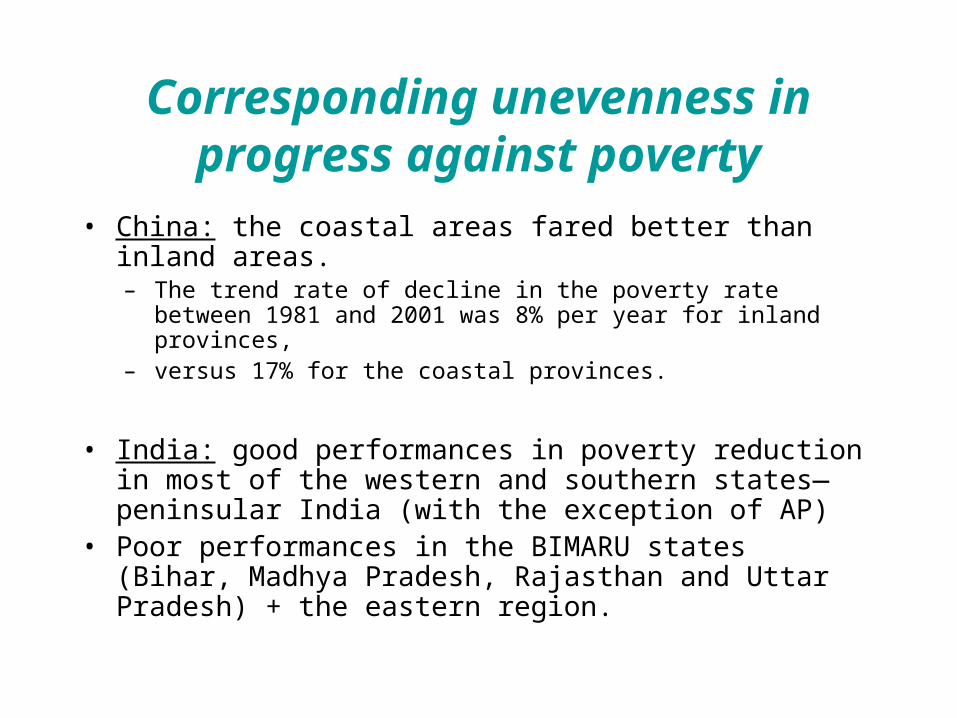
Corresponding unevenness in progress against poverty

• China: the coastal areas fared better than inland areas. – The trend rate of decline in the poverty rate between 1981 and

2001 was 8% per year for inland provinces, – versus 17% for the coastal provinces.

• India: good performances in poverty reduction in most of the western and southern states—peninsular India (with the exception of AP)

• Poor performances in the BIMARU states (Bihar, Madhya Pradesh, Rajasthan and Uttar Pradesh) + the eastern region.

Higher growth was not found where it would have the most impact on poverty

0

1

2

3

4

5

6

7

- .8 - .7 - .6 - .5 - .4 - .3 - .2 - .1 .0 .1

S h are w e igh ted to ta l e las tic ity o f th e h e adc ou n t in d ex to g row th

Tre

nd

ra

te o

f g

row

th in

me

an

ru

ral i

nco

me

(%

/ye

ar)

H e n an

2

4

6

8

10

12

14

-0.14 -0.12 -0.10 -0.08 -0.06 -0.04 -0.02 0.00

Impact on national poverty of non-farm output growth by state (Share–weighted elasticity for 1993/94)

Gro

wth

rat

e in

non

-far

m o

utpu

t per

cap

ita

199

3/94

-199

9/0

0 (%

/yea

r)

China India

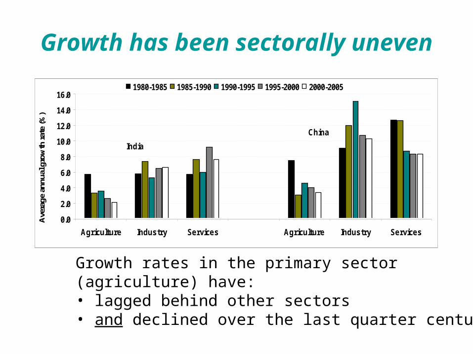
Growth has been sectorally uneven

India

China

0.0

2.0

4.0

6.0

8.0

10.0

12.0

14.0

16.0

Agriculture Industry Services Agriculture Industry Services

Ave

rage

ann

ual g

row

th ra

te (%

)

1980-1985 1985-1990 1990-1995 1995-2000 2000-2005

Growth rates in the primary sector (agriculture) have:• lagged behind other sectors • and declined over the last quarter century

+ uneven between urban and rural areas

• China: trend increase in ratio of urban to rural mean over 1981-2002– This is greatly reduced allowing for higher urban inflation rate

– But rising trend is still evident since mid-1990s.

• India: trend increase in ratio of urban to rural mean consumption since 1980s

• Mean income: • Growth rate:

• Test equation:

• Null hypothesis:

ut

ut

rt

rtt nn

rt

ut

rt

ut

rt

ut

ut

rt

rtt nnnssss ln)]/([lnlnln

tit

it

it ns /

trtu

t

rtu

trt

n

ut

ut

urt

rt

rt

nn

nss

ssP

ln).(

lnlnln 0

H0: i for i=r,u,n

Do sectoral imbalances matter to the rate of poverty reduction?Regression decomposition test

China India

-2.56 -1.46 Growth rate of mean rural income (share-

weighted) (-8.43) (12.64)

0.09 -0.55 Growth rate of mean urban income

(share-weighted) (0.20) (-1.37)

0.74 -4.46 Population shift effect (0.16) (-1.31)

R2 0.82 0.90

Poverty reduction and the urban-rural composition of growth

trtu

t

rtu

trt

nut

ut

urt

rt

rt n

n

nssssP ln).(lnlnln 0

Sectoral imbalances matter to the rate of poverty reduction

China India

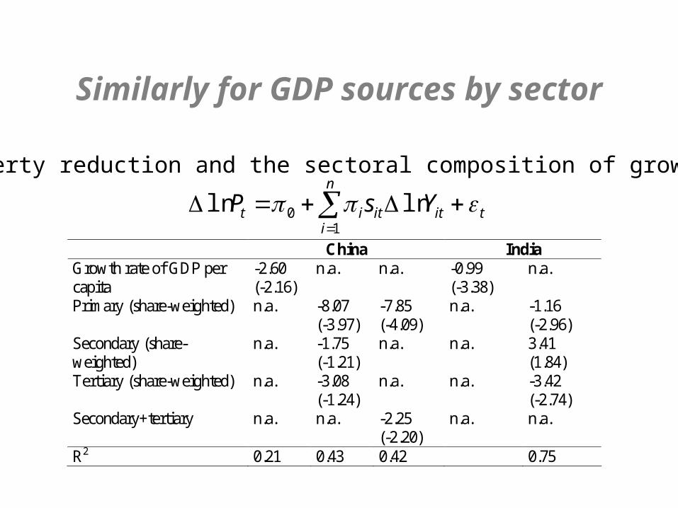
-2.60 n.a. n.a. -0.99 n.a. Growth rate of GDP per capita (-2.16) (-3.38)

n.a. -8.07 -7.85 n.a. -1.16 Primary (share-weighted) (-3.97) (-4.09) (-2.96) n.a. -1.75 n.a. n.a. 3.41 Secondary (share-

weighted) (-1.21) (1.84) n.a. -3.08 n.a. n.a. -3.42 Tertiary (share-weighted) (-1.24) (-2.74) n.a. n.a. -2.25 n.a. n.a. Secondary+tertiary (-2.20)

R2 0.21 0.43 0.42 0.75

t

n

iititit YsP

10 lnln

Poverty reduction and the sectoral composition of growth

Similarly for GDP sources by sector

Uneven growth has contributed to rising inequality

• Differing initial conditions– Lower inequality of agricultural land holding in China

– Also lower inequalities in human capital in China

– Larger urban-rural inequality in China

• China: Primary sector growth has been inequality decreasing; secondary and tertiary have had no effect.

• A (moving average) growth rate of 7.0% p.a. would be needed to avoid rising inequality whereas the mean primary-sector growth rate was under 5% between 1981 and 2001.

Gtttt YYG ̂2/)lnln(746.00522.0ln 111

)723.3()563.4(

Why should we care about uneven growth?

What should be done about it?

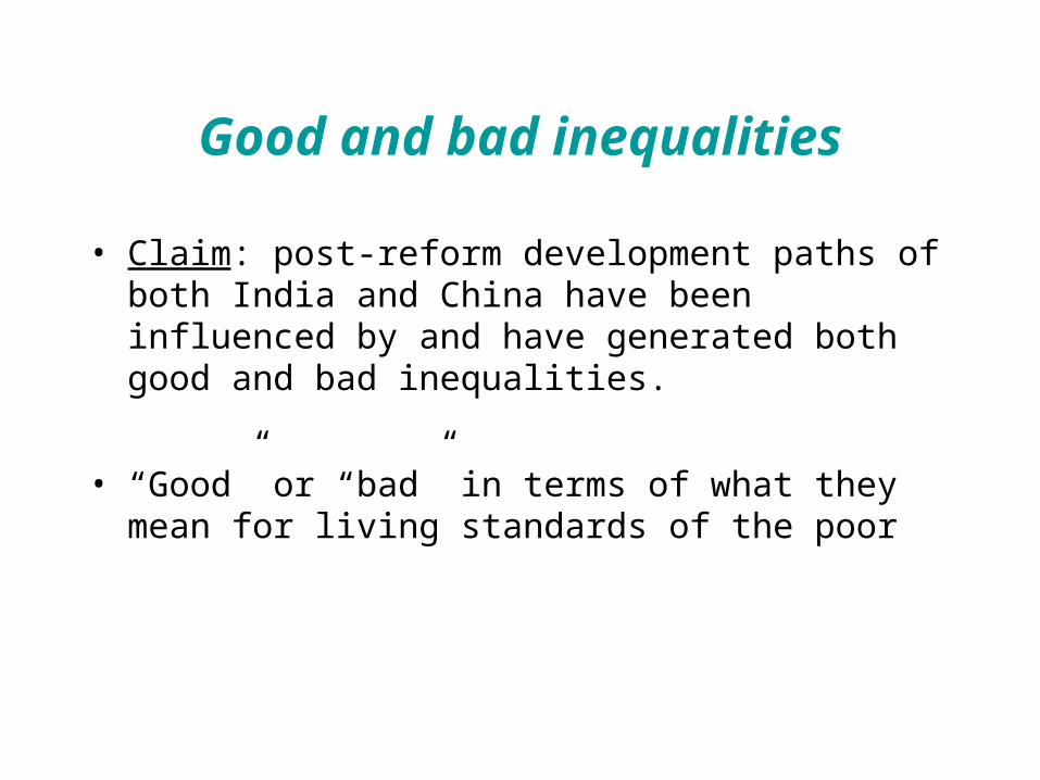
Good and bad inequalities

• Claim: post-reform development paths of both India and China have been influenced by and have generated both good and bad inequalities.

• “Good” or “bad” in terms of what they mean for living standards of the poor

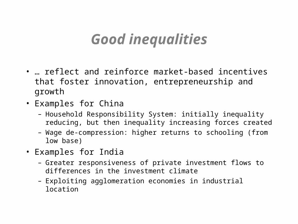
Good inequalities

• … reflect and reinforce market-based incentives that foster innovation, entrepreneurship and growth

• Examples for China– Household Responsibility System: initially inequality reducing,

but then inequality increasing forces created

– Wage de-compression: higher returns to schooling (from low base)

• Examples for India– Greater responsiveness of private investment flows to differences

in the investment climate

– Exploiting agglomeration economies in industrial location

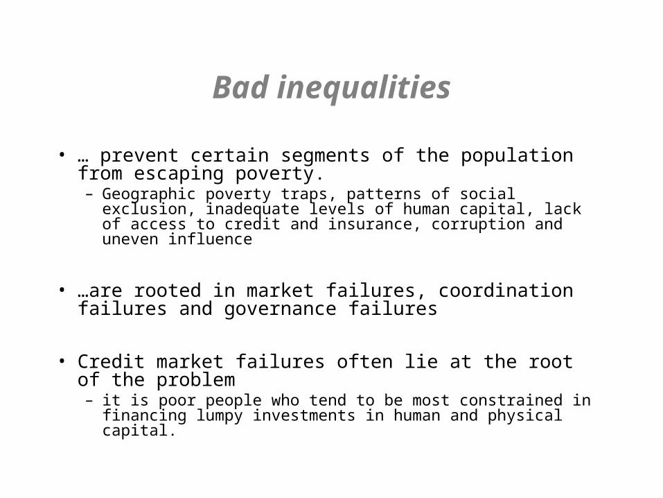
Bad inequalities

• … prevent certain segments of the population from escaping poverty. – Geographic poverty traps, patterns of social exclusion, inadequate

levels of human capital, lack of access to credit and insurance, corruption and uneven influence

• …are rooted in market failures, coordination failures and governance failures

• Credit market failures often lie at the root of the problem – it is poor people who tend to be most constrained in financing

lumpy investments in human and physical capital.

Example 1:

Geographic poverty traps

• Living in a well-endowed area entails that a poor household can eventually escape poverty, while an otherwise identical household living in a poor area sees stagnation or decline.

• In both countries, initially poorer provinces saw lower subsequent growth.

• China: Evidence of geographic externalities stemming from both publicly-controlled endowments (such as the density of rural roads) and largely private ones (such as the extent of agricultural development locally).*

* Jalan, Jyotsna and Martin Ravallion, “Geographic Poverty Traps? A Micro Model of Consumption Growth in Rural China?” Journal of Applied Econometrics, 2002, Vol. 17, pp. 329–46.

Example 2:

Inequalities in human capital

• …are a key factor impeding pro-poor growth in both countries.

• China: Widespread basic schooling at the outset of the reform period

• But rising inequalities over time threaten current and future prospects for both growth and poverty reduction.

• India: Long-standing inequalities in schooling (higher than in China) that have retarded the pace of poverty reduction at given growth rates, esp., from non-farm economic growth.

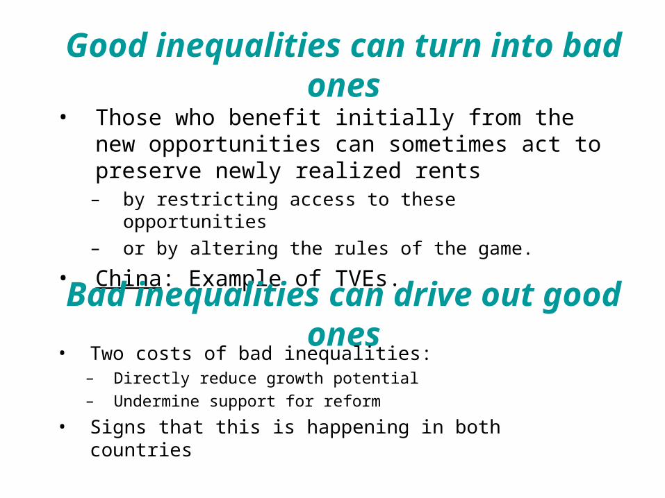
Good inequalities can turn into bad ones

• Those who benefit initially from the new opportunities can sometimes act to preserve newly realized rents

– by restricting access to these opportunities

– or by altering the rules of the game.

• China: Example of TVEs.

Bad inequalities can drive out good ones• Two costs of bad inequalities:

– Directly reduce growth potential

– Undermine support for reform

• Signs that this is happening in both countries

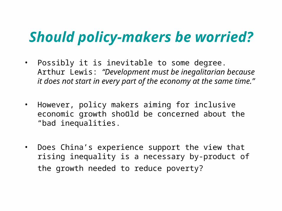
Should policy-makers be worried?

• Possibly it is inevitable to some degree. Arthur Lewis: “Development must be inegalitarian because it does not start in every part of the economy at the same time.”

• However, policy makers aiming for inclusive economic growth should be concerned about the “bad inequalities.”

• Does China’s experience support the view that rising inequality is a necessary by-product of the growth needed

to reduce poverty?

China: Surprisingly little sign of an aggregate growth-equity trade off

• The strong positive correlation over time between China’s GDP per capita and inequality is driven by common time trends.

• Near zero correlation between changes in (log) Gini and growth rate.

• The periods of more rapid growth did not bring more rapid increases in inequality. Indeed,…

Annualized log difference (%/year)

Inequality

Gini index

Mean household

income

GDP per

capita

1. 1981-85 Falling -1.12 8.87 8.80 2. 1986-94 Rising 2.81 3.10 7.99 3. 1995-98 Falling -0.81 5.35 7.75 4. 1999-2001 Rising 2.71 4.47 6.61

The periods of falling inequality had highest growth in mean household income

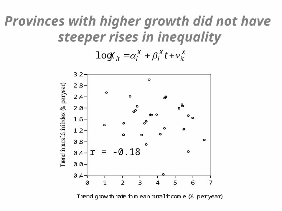
-0.4

0.0

0.4

0.8

1.2

1.6

2.0

2.4

2.8

3.2

0 1 2 3 4 5 6 7

Trend growth rate in mean rural income (% per year)

Tre

nd in

rur

al G

ini i

ndex

(%

per

yea

r)

Provinces with higher growth did not have steeper rises in inequality

r = -0.18

Xit

Xi

Xiit tX log

Double handicap in unequal provinces

More unequal provinces faced two handicaps in rural poverty reduction in China:

1. High inequality provinces had a lower growth elasticity of poverty reduction:

At zero trend in inequality, (mean) growth elasticity is zero at maximum inequality and -6 at minimum inequality

2. High inequality provinces had lower growth:

Signs of “inefficient inequality” both within rural areas, and between urban and rural areas =>tG

iR

iR

iY

iH

i Gy ˆ365.1)1)(0136.0935.5(/)392.2(

8380)560.2()487.4(

R 2 = 0 . 3 8 6 ; n = 2 9

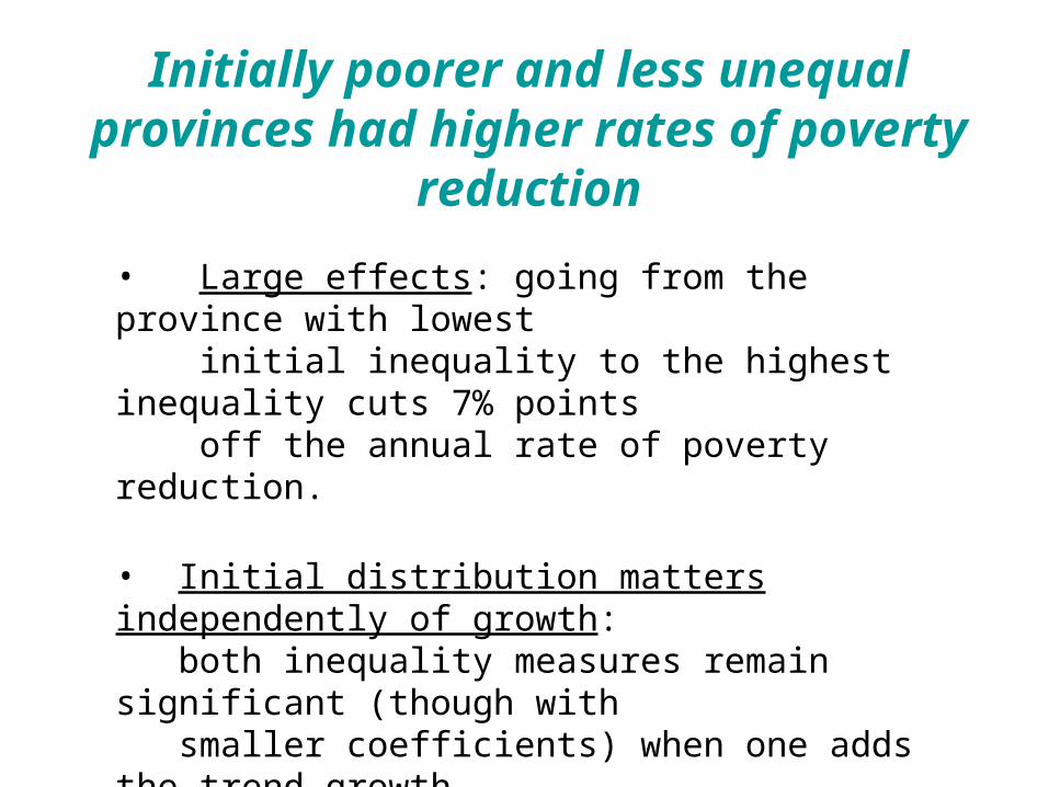
Initially poorer and less unequal provinces had higher rates of poverty reduction

• Large effects: going from the province with lowest initial inequality to the highest inequality cuts 7% points off the annual rate of poverty reduction.

• Initial distribution matters independently of growth: both inequality measures remain significant (though with smaller coefficients) when one adds the trend growth rate to the regression for trend poverty reduction

Regressions for provincial trends

tii

iR

iiH

i

GDONGCOAST

URGY

ˆ012.25291.9

797.6463.0141.0877.67

)160.15()292.5(

)201.3(83

)313.3(80

)090.8()239.6(

R 2 = 0 . 8 2 7

tii

iR

iiY

i

GDONGCOAST

URGY

ˆ290.1507.0

632.1149.0007.0143.14

)875.1()913.0(

)682.2(83

)526.2(80

)294.1()759.3(

R 2 = 0 . 4 2 3

Initial conditions (mean and distribution) + location

Initial ratioof urban meanto rural mean

Initial Gini index

Inequality is now an issue for China

• High inequality in many provinces will inhibit future prospects for both growth and poverty reduction.

• Aggregate growth is increasingly coming from sources that bring limited gains to the poorest.

• Inequality is continuing to rise and poverty is becoming much more responsive to rising inequality.

• Perceptions of what “poverty” means are also changing, which can hardly be surprising in an economy that can quadruple its mean income in 20 years.

Elasticity of poverty rate to

Gini index 1981 0.0 2001 3.7

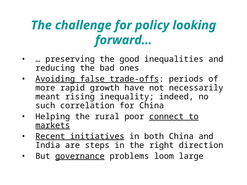
The challenge for policy looking forward…

• … preserving the good inequalities and reducing the bad ones

• Avoiding false trade-offs: periods of more rapid growth have not necessarily meant rising inequality; indeed, no such correlation for China

• Helping the rural poor connect to markets• Recent initiatives in both China and India are steps in the

right direction• But governance problems loom large