performance analysis and tuning in multicore environments · performance analysis and tuning in...
TRANSCRIPT

Computer Architecture and Operative Systems Department
Master in High Performance Computing
Performance Analysis and Tuning in Multicore Environments
2009
MSc research Project for the “Master in
High Performance Computing” submitted
by MARIO ADOLFO ZAVALA JIMENEZ,
advised by Eduardo Galobardes.
Dissertation done at Escola Tècnica
Superior d’Enginyeria (Computer
Architecture and Operative Systems
Department).


Abstract
Performance analysis is the task of monitor the behavior of a program execution. The
main goal is to find out the possible adjustments that might be done in order improve the
performance. To be able to get that improvement it is necessary to find the different causes
of overhead. Nowadays we are already in the multicore era, but there is a gap between the
level of development of the two main divisions of multicore technology (hardware and
software). When we talk about multicore we are also speaking of shared memory systems,
on this master thesis we talk about the issues involved on the performance analysis and
tuning of applications running specifically in a shared Memory system. We move one step
ahead to take the performance analysis to another level by analyzing the applications
structure and patterns. We also present some tools specifically addressed to the
performance analysis of OpenMP multithread application. At the end we present the results
of some experiments performed with a set of OpenMP scientific application.
Keywords: Performance analysis, application patterns, Tuning, Multithread, OpenMP,
Multicore.

Resumen
Análisis de rendimiento es el área de estudio encargada de monitorizar el
comportamiento de la ejecución de programas informáticos. El principal objetivo es
encontrar los posibles ajustes que serán necesarios para mejorar el rendimiento. Para poder
obtener esa mejora es necesario encontrar las principales causas de overhead. Actualmente
estamos sumergidos en la era multicore, pero existe una brecha entre el nivel de desarrollo
sus dos principales divisiones (hardware y software). Cuando hablamos de multicore
también estamos hablando de sistemas de memoria compartida. Nosotros damos un paso
más al abordar el análisis de rendimiento a otro nivel por medio del estudio de la estructura
de las aplicaciones y sus patrones. También presentamos herramientas de análisis de
aplicaciones que son específicas para el análisis de rendimiento de aplicaciones paralelas
desarrolladas con OpenMP. Al final presentamos los resultados de algunos experimentos
realizados con un grupo de aplicaciones científicas desarrolladas bajo este modelo de
programación.
Palabras claves: Análisis de rendimiento, Patrones de la aplicación, Sintonización,
Multithread, OpenMP, Multicore.

Resum
L’Anàlisi de rendiment és l'àrea d'estudi encarregada de monitorizar el comportament
de l'execució de programes informàtics. El principal objectiu és trobar els possibles
ajustaments que seran necessaris per a millorar el rendiment. Per a poder obtenir aquesta
millora és necessari trobar les principals causes de l’overhead (excessos de computació no
productiva). Actualment estem immersos en l'era multicore, però existeix una rasa entre el
nivell de desenvolupament de les seves dues principals divisions (maquinari i programari).
Quan parlam de multicore, també estem parlant de sistemes de memòria compartida.
Nosaltres donem un pas més per a abordar l'anàlisi de rendiment en un altre nivell per mitjà
de l'estudi de l'estructura de les aplicacions i els seus patrons. També presentem eines
d'anàlisis d'aplicacions que són específiques per a l'anàlisi de rendiment d'aplicacions
paral·leles desenvolupades amb OpenMP. Al final, presentem els resultats d'alguns
experiments realitzats amb un grup d'aplicacions científiques desenvolupades sota aquest
model de programació.
Paraules claus: Anàlisis de rendiment, Patrons de l'aplicació, Sintonització, Multithread,
OpenMP, Multicore.
Contents
1 Introduction .............................................................................................................. 9
1.1 General Overview ................................................................................................ 9
1.2 Objectives .......................................................................................................... 10
1.3 Contribution....................................................................................................... 10
1.4 Problems definition ............................................................................................ 11
1.5 State of Art ........................................................................................................ 11
2 Multicore Technology ............................................................................................ 17
2.1 General overview ............................................................................................... 17
2.2 Core count and its complexity ............................................................................ 18
2.3 Heterogeneity vs homogeneity ........................................................................... 19
2.4 Memory Hierarchy and interconnection ............................................................. 20
3 Multithread Applications in Multicore Environments ......................................... 24
3.1 Study cases with multithread applications .......................................................... 24
3.1.1 N-body ....................................................................................................... 27
3.1.2 Molecular Dynamics ................................................................................... 28
3.1.3 Fast Fourier Transform ............................................................................... 30
3.2 Programming models ......................................................................................... 33
3.2.1 Pthreads ...................................................................................................... 34
3.2.2 OpenMP ..................................................................................................... 36
3.2.3 Cilk............................................................................................................. 39
3.2.4 The Intel threading building blocks (TBB) .................................................. 41
3.2.5 Java Threads ............................................................................................... 44
4 Performance analysis and Tuning ......................................................................... 47
4.1 Key factors to improve the performance............................................................. 47
4.1.1 Coverage and Granularity ........................................................................... 47
4.1.2 Synchronization .......................................................................................... 49
4.1.3 Memory access patterns .............................................................................. 50
4.1.4 Inconsistent parallelization .......................................................................... 52
4.1.5 Loop optimization ....................................................................................... 52
4.1.6 Dynamic threads ......................................................................................... 55
4.2 Performance Analysis tools evaluated ................................................................ 57
4.2.1 PAPI ........................................................................................................... 58
4.2.2 OMPP ......................................................................................................... 61
5 Experiments ............................................................................................................ 68
5.1 Hardware configuration ..................................................................................... 68
5.2 First group of experiment: Importance of application parallel structure .............. 69
5.2.1 Methodology .............................................................................................. 70
5.2.2 Explanation ................................................................................................. 70
5.2.3 Results ........................................................................................................ 75
5.3 Second group of experiment: Scalability in OpenMP multithread applications. .. 78
5.3.1 Methodology .............................................................................................. 78
5.3.2 Results ........................................................................................................ 78
6 Conclusions and future work ................................................................................. 82
6.1 Conclusions ....................................................................................................... 82

6.2 Future work ....................................................................................................... 83
References ...................................................................................................................... 84

Acknowledgments
I want to thanks the people and institution that has support to achieve this master
research project. I want to thank Univertat Autònoma de Barcelona for promoting the
education of new researchers in different fields, especially in the field of High Performance
Computing.
I would like to express my gratitude to the staff of professor of the department of
Computer Architecture and Operating Systems (CAOS) of Universitat Autonoma for give
me the opportunity to belong to their work and for all our advices and correction which has
been always welcome and appreciated from my part, especially I want to thanks my master
thesis directors, Drs. Eduardo Galobardes, Josep Jorba and my research tutor Dr. Tomàs
Margalef for their guidance and time during this period of research.
Thanks you to Dr. Emilio Luque and Lola Isabel Rexachs for being always taking care
of our group of researchers not only as supervisors, but also as supporters in our daily work
and problems.
Thanks to my family for supporting me always in distance and be waiting for me to go
back home when an opportunity appears. They are the main supporters in my professional
life.
Finally but not less important I would like to thank my laboratory partners for let me
be part of this group, for your friendship, advices and knowledge.
Thank you very much,

9
1 Introduction
1.1 General Overview
Performance analysis is the task of monitor the behavior of a program execution. The
main goal is to find out the possible adjustments that might be done in order improve the
performance. Besides, the hardware architecture and software platform (operative system)
where the program is being executed play an important role on the program performance.
Nowadays multicore processors chips are being introduced in almost all the areas where a
computer is needed. For example, a common laptop computer with a dual core processor
inside. High Performance Computing (HPC) address different issues, one of them is to
exploit the capacities of multicore architecture.
Performance analysis and tuning is a field of HPC responsible of analyzing the
behavior of applications that perform a big amount of computation. Some applications that
require a high volume of computation require analyzing and tuning. Therefore, in order to
achieve a better performance it is necessary to find the different causes of overhead.
There are a considerable number of studies related to the performance analysis and
tuning of applications for supercomputing, but there are relatively few studies addressed
specifically to applications running on a multicore environment. A multicore environment
is a computer with a particular kind of processors which have two or more independent
cores integrated in one chip. Those processors have also other singular characteristics such
as their memory hierarchy or internal core interconnection.
A multicore processor is a processing system composed of two or more independent
cores (or CPUs). The cores are typically integrated onto a single integrated circuit die
(known as a chip multiprocessor or CMP), or they may be integrated onto multiple dies in
a single chip package.
On this master thesis we will talk about the issues involved on the performance
analysis and tuning of applications running specifically in a shared Memory system.

10
Multicore hardware is relatively more mature than multicore software, from that reality
arises the necessity of this research. We would like to emphasize that this is an active area
of research, and there are only some early results in the academic and industrial worlds in
terms of established standards and technology, but much more will evolve in the years to
come.
1.2 Objectives
The main objective of this research is to analyze and monitor the performance
execution of multithread applications specifically running in a multicore environment. In
this case we are addressing the specific case of OpenMP multithread applications. From
that analysis we will be able to know the behavior, execution patterns and main causes of
overhead on this environment in order to apply the necessary measures/changes to make a
better use of the hardware resources and therefore obtain a better performance.
To achieve our objective we haven`t followed the general model where the analysis of
the application is done taking the application as a black box. Our work differs from the
general model in that, doing the analysis on that way might be sometimes more difficult
due to the lack of knowledge of the application’s task flow. Therefore we have gone one
step ahead in the analysis of the applications through extraction the applications structure
and execution patterns.
We aim to know the specific characteristics of multithread application in order to know
the most suitable manner to run a multithread application in a multicore environment. To
do so, we have performed a set of experiments to help us to extract the information
required to build a performance model.
1.3 Contribution
The main contribution of this master thesis is the characterization of the execution of a
set of scientific multithread applications. We also contribute by creating an analysis

11
environment addressed specifically to scientific multithread applications that might help
most to the analysis of this type of applications.
1.4 Problems definition
Multicore hardware technology is advancing very fast. There is a gap between the level
of development of the multicore hardware and multicore software technology.
Multithread applications may not always take proper advantage of multicore hardware
architecture. If the parallel application is not well optimized or the design gives additional
burden to the execution task, we might fall in the case that a single thread application runs
faster than multithread applications. Sometimes it is not enough to add the basic directives
to make an application run faster in its parallel version. It is necessary to be aware of
application structure and execution patterns in order to address this problem.
On a shared-memory multiprocessor system, the adverse impact is even stronger. The
more threads involved, the bigger the potential performance problem. The reason is that a
miss at the highest cache level causes additional traffic on the interconnection system. No
matter how fast this interconnection is, parallel performance degrades because none of the
systems on the market today have an interconnection with sufficient bandwidth to sustain
frequent cache misses simultaneously by all processors (or cores) in the system. That
problem is solve in part with hierarchy memory which implicate to place different levels de
cache memory.
There are many issues that we must to consider. In this master thesis we address those
problems by the performance analysis and tuning for this specific type of applications in
specific hardware architecture.
1.5 State of Art
The multicore technology may be divided into two main categories, hardware and
software. Multicore software is a new field that is emerging from the necessity of obtaining
a good performance on multicore processors. The goal in multicore software field is to take
12
advantage from multicore hardware as much as possible. But that goal is not an easy task;
we need to parallelize the application which at the same time makes the software more
complicated, error prone and thus expensive. So far, there is not a unique standard
programming model to follow with many proposals to analyze and test. Those proposals
start from keeping the sequential model and using automatic parallelization to
programming with a low level threads interface. In the latter case, debugging becomes
much more difficult due to the inherently nondeterministic nature of multithreaded
programming.
With the emergence of multicore computers, software engineers face the challenge of
parallelizing performance-critical applications of all sorts. Compared to sequential
applications, our repertoire of tools and methods for cost-effectively developing reliable,
fault tolerant, robust parallel applications is irregular.
The roadmaps of the semiconductor industry predict several hundreds of cores per chip
in future generations. This development presents an opportunity that the software industry
cannot ignore. The bad news is that the era of doubling performance every 18 months has
come to an end [1]. This means that the implicit performance improvement \for free" with
every chip generation has also ended. Thus, future performance gains, required for new or
improved applications, will have to come from parallelism. Unfortunately, one cannot rely
solely on compilers to perform the parallelization work, as the choice or parallelization
strategy has a significant impact on performance and often requires massive program
refactoring. Software engineering now faces the problem of developing parallel
applications, while keeping cost and quality of software constant [2].
There are several programming models that have been proposed for multicore processors.
These models are not new, but go back to models proposed for multichip multiprocessors.
Shared memory models assume that all parallel activities can access all of memory.
Communication between parallel activities is through shared mutable state that must be
carefully managed to ensure correctness. Various synchronization primitives such as locks
or transactional memory is used to enforce this management.

13
Message passing models eschew shared mutable state as a communications medium in
favor of explicit message passing, typically used to program clusters, where the distributed
memory of the hardware maps well to the models lack of shared mutable state.
In between these two extremes there are partitioned global address space models where the
address space is partitioned into disjoint subsets such that computations can only access
data in the subspace in which they run (as in message passing) but they can hold pointers
into other subsets (as in shared memory).
Most models that have been proposed for multicore fall in the shared memory class [2].
Related work
Nowadays, the related research that is being done may be classified into the following
topics which are addressed by multicore software engineers around the world.
• Parallel patterns
• Frameworks and libraries for multicore software
• Parallel software architectures
• Modeling techniques for multicore software
• Software components and composition
• Programming languages/models for multicore software
• Compilers for parallelism
• Testing and debugging parallel applications
• Parallel algorithms and data structures
• Software reengineering for parallelism
• Transactional Memory
• Auto tuning
• Operating system support, scheduling
• Visualization tools
• Development environments for multicore software
• Process models for multicore software development

14
• Experience reports from research or industrial projects
• Fault tolerance techniques
• Execution monitoring with multicore
The information related to our research comes from many contributions done by
researcher in those different topics, there are a considerable number of international
workshops which groups those works and permits researcher to exchange experiences and
valuable information.
Another example of related work is the one done by The Multicore Association which
is an open membership organization that includes leading companies implementing
products that embrace multicore technology. Their members represent vendors of
processors, operating systems, compilers, development tools, debuggers, ESL/EDA tools,
simulators, as well as application and system developers, and share the objective of
defining and promoting open specifications [3].
One of the most important projects doing research on this area is the Jülich
Supercomputing Centre (JSC). This projects provides supercomputer resources, IT tools,
methods and knowhow for the Research Centre Jülich and for European users through the
John von Neumann Institute for Computing. The most known tool provided by JSC is
called Scalasca, this tools offers a very good approach for performance analysis on hybrid
MPI-OpenMP application. The version which is going to support pure OpenMP
applications performance analysis is being developed. JSC has also another important
project called APART [31] which is a forum of tool experts, parallel computer vendors, and
software companies to discuss automation of performance analysis tools. Its goal is to
identify.
• Requirements for automatic performance analysis support
• Knowledge about typical performance bottlenecks
• Base implementation technologies
The APART group defined the APART Specification Language (ASL) for writing
portable specifications of typical performance problems [4]. ASL allows specifying
performance-related data by an object-oriented model and performance properties by

15
functions and constraints defined over performance-related data. Performance problems
and bottlenecks can then be identified based on user- or tool-defined thresholds. In order to
demonstrate the usefulness of ASL they apply it to OpenMP by successfully formalizing
several OpenMP performance properties.
There is also a set of performance analysis tools which aims to help solving the
problem of performance analysis for multithread applications. Some examples of those
tools are ompP, mpiP, HPCToolkit, PerfSuite, PapiEx, GPTL, pfmon, TAU, Scalasca,
valgrind, gprof, Non-OS, Vampir, SlowSpotter. In our research we have interacted with the
most of them, being ompP and PAPI the most suitable tools specifically for our research,
however, we are still interacting and evaluating more tools in order to obtain the most
suitable information during our experiments.
What we do?
In our research we try to address many of multicore topic mentioned before, the following
is a description of what we do and what we don’t do.
• Our research is focused in the performance analysis and tuning of OpenMP multi-
thread applications running specifically in multicore processors hardware
architecture.
• Multicore processors have different levels of shared and no-shared memory caches.
Therefore we only analyze the issues regarding shared memory.
• We have introduced ourselves to different programming models for shared memory
multithread applications; however, we have begun our experiments with the most
popular model called OpenMP. Experiments with applications developed with other
models will be performed in the future.
• So far we are focused on homogeneous multicore processors. The case of
heterogeneous multicore processors might be addressed later.
• We state that the performance analysis of multithread applications cannot always be
addressed considering the applications as a black box. It is necessary to go deeper

16
and analyze the application’s structure in order to extract important information
about its structure and organization. Some useful information might be the number
of parallel regions, the memory access pattern, type of data distribution
(scheduling), nested loops and others.
• As a general objective for in our research, we aim to produce a performance model
for multithread applications running in muliticore environment. We divide our
research into two stages. The master course and the PhD course stages. A
performance model is an objective for Phd course, in the other hand, for this master
thesis we have specific goals and products.
• The final product of this master thesis is model of key factors that affect the
performance of OpenMP a group of OpenMP multithread application. This work
will serve a base to create a more general performance model in the next stage of
our research.
• For Phd course we expect to cover more aspect regarding this subject. We also
expected to explore the rest of programming models and tools.

17
2 Multicore Technology
2.1 General overview
Since several years ago, the computer technology has been going through a phase of
many changes. Based on Moore law, the speed of processors was increasing very fast.
Every new generation of micro-processors had the clock rate usually twice or even much
faster than the previous one. That increase in clock frequency drove increases in the
processors performance, but at the same time, the difference between the processors speed
and memory speed was increasing. That gap was temporarily solved by instruction level
parallelism (ILP) [2]. Exploiting ILP means executing instructions that occur close to each
other in the stream of instructions through the processor in parallel. Though it appeared
very soon that more and more cycles are being spent not in the processor core execution,
but in the memory subsystem which includes the multilevel caching structure, and the so-
called Memory Wall problem started to evolve quite significantly due to the fact that the
increase in memory speed didn’t match that of processor cores.
Very soon a new direction for increasing the overall performance of computer systems
had been proposed, namely changing the structure of the processor subsystem to utilize
several processor cores on a single chip. These new computer architectures received the
name of Chip Multi Processors (CMP) and allowed to provide increased performance for
new generation of systems, while keeping the clock rate of individual processors cores at a
reasonable level. The result of this architectural change is that it is possible to provide
further improvements in performance while keeping the power consumption of the
processor subsystem almost constant, the trend which appears essential not only to power
sensitive market segments such as embedded systems, but also to computing server farms
which suffer of power consumption/dissipation problems as well.
A multicore processor or chip multi-processor CMP is an emerging processor technology
which combines two or more independent processors into a single package [5]. Inside a
CMP there is a memory hierarchy that could vary from one model to another. This
technology is becoming more used day by day in all the areas of computing. Some of the
advantages that shared memory CMP may offer are:

18
• Direct access to data through shared memory address space.
• Great latency hiding mechanism.
• MP’s appears to lower power and cooling requirements per FLOP.
There are two main type of CMP, First, there are those that contain a few very
powerful cores, essentially the same core one would put in a single core processor.
Examples include AMD Athlons, Intel Core 2, IBM Power 6 [14] and so on. Second, there
are those systems that trade single core performance for number of cores, limiting core area
and power. Examples include the Tilera 64, the Intel Larrabee [19]and the Sun
UltraSPARC T1 [2]and T2 (also known as Niagara 1-2). Figure 2.1 shows the basic
structure of a dual core processor.[multicore the state of art]. Next we provide a better
explanation of these types of CMP.
Fig. 2-1. An example of a dual core MCP structure.
2.2 Core count and its complexity
The marked divides its offer based on the expected speedup from additional cores [2].
First is the market where a considerable part of the running applications code is not
parallelized, such as desktops/laptops systems, speedup from extra cores is less than linear
and may frequently be zero [2]. It means that an additional core will not necessary provide
more efficiency. In the other hand, there a market where the expected speedup from extra

19
cores is assumed to be linear. In this case the situation is different. Under this expectation,
core design should follow the KILL rule.
The Kill Rule [6] is a simple scientific way of making the tradeoff between increasing
the number of cores or increasing the core size. The Kill Rule states that a resource in a
core must be increased in area only if the core’s performance improvement is at least
proportional to the core’s area increase. Put another way, increase resource size only if for
every 1% increase in core area there is at least a 1% increase in core performance.
2.3 Heterogeneity vs homogeneity
In a multicore chip, the cores could be identical or there could be more than one kind of
core. Our research is focused on a homogeneous multicore environment. But we consider
important to explain the differences between homogeneous and heterogeneous CMP. There
are two levels of heterogeneity depending on whether the cores have the same instruction
set or not. Hence there are three possibilities [2]:
• Identical cores, as in most current multicore chips from the Intel Core 2 to the
Tilera 64.
• Cores implementing the same instruction set but with different nonfunctional
characteristics.
• Cores with different instruction sets like in the Cell processor where one core
implements the PowerPC architecture and 6-8 synergistic processing elements
implement a different RISC instruction set.

20
Fig. 2-2. A basic homogenous Chip Multiprocessor
Fig. 2-3. An example of a heterogeneous Chip Multiprocessor
2.4 Memory Hierarchy and interconnection
One of the major challenges facing computer architects today is the growing
discrepancy in processor and memory speed [7]. Processors have been consistently getting
faster. But the more rapidly they can perform instructions, the quicker they need to receive
the values of operands from memory. Unfortunately, the speed with which data can be read
from and written to memory has not increased at the same rate. Memory access time is
increasingly the bottleneck in overall application performance. As a result, an application
might spend a considerable amount of time waiting for data. This not only negatively

21
impacts the overall performance, but the application cannot benefit much from a processor
clock-speed upgrade either.
In response, the vendors have built computers with hierarchical memory systems, in
which a small, expensive, and very fast memory called cache memory, or “cache” for short,
supplies the processor with data and instructions at high rates [8]. Each processor of a
shared memory system needs its own private cache if it is to be fed quickly; hence, not all
memory is shared.
Most programs have a high degree of locality in their accesses. Memory hierarchy tries
to exploit locality. There two types of locality:
• Spatial locality: When accessing things nearby previous accesses
• Temporal locality: When reusing an item that was previously accessed.
Figures 2-4 and 2-5 show an example the organization of processors memory hierarchy.
Figure 2-4 shows the organization with two levels of cache memory. Nowadays an
additional level (level 3) is used in many multicore processors.
Fig. 2-4 Memory access hierarchy organization of general processors units.

22
Fig. 2-5. Estimation of speed accesses scale in a processor unit.
One salient characteristic of multicore architectures is that they have a varying degree
of sharing of caches at different levels. Most of the architectures have cores with a private
L1 cache. Depending on the architecture, an L2 cache is shared by two or more cores; and
an L3 cache is shared by four or more cores. The main memory is typically shared by all
cores. The degree of sharing at a level varies from one multicore processor to another.
When we speak of CMP we are speaking of shared memory at some levels. Most
multicore designs provide some form of coherent caches that are transparent to software.
First level caches are typically private to each core and split into instruction and data
caches, as in the preceding generation of single core processors [2].
• Early dual core processors had private per core second level caches and were
essentially a double single core processor with a minimum of glue logic and an
essentially snooping coherence protocol. Some designs continue with separate L2
caches, like the Tilera 64 where each core has a 64 KB L2 cache. However, the
glue logic is in this case anything but simple and amounts to a directory based
cache coherency protocol on a mesh interconnect.

23
• Second level caches can be shared between the cores on a chip; this is the choice in
the Sun Niagara (a 3MB L2 cache) as well as the Intel Core 2 Duo (typically 2-6
MB).
• Separate L2 caches backed by a shared L3 cache as in the AMD Phenom processor
(512 KB L2 per core, shared 2MB L3) or the recent Intel Core i7 (256 KB L2 per
core, shared 8MB L3).
• A hierarchy where L2 caches are shared by subsets of cores. This pertains to the
four core Intel Core 2 Quad, which is essentially two Core 2 Duo in a single
package. Each of the chips have an L2 cache shared between its two cores but the
chips have separate caches.
With private L2 caches, the L1-L2 communication is local, and the intercore
interconnect is located below the L2 cache, whereas with a shared L2 it sits between the L1
and L2 caches. In the shared case, all L1 misses go over the interconnect whereas in the
private case only those that also miss in the L2 do so. This requires a more expensive, low
latency interconnect (often a crossbar) which uses a lot of area that could otherwise be used
for larger caches (or morecores). Also, L2 access time is increased by the need to go over
the interconnect [2].
On the other hand, private L2 caches might waste chip area by having the same data
occupy space in several caches, and accessing data in the L2 of another core, something
that is sometimes needed to achieve cache coherency, becomes more expensive than
accessing a shared L2 cache.

24
3 Multithread Applications in Multicore Environments
On this chapter we addressed the concepts of multithread application and multicore
processors in order to allow the lector to have a good conceptual base of the subject we are
addressing on this master thesis. We also explain the theory of three scientific applications
that we will use to perform our experiments. Finally we provide an overview of the main
programming models used for multithread applications nowadays. Even though in this
master thesis we are focusing on OpenMP programming model, it is important to
understand at what level of parallelism we are working when using one of those
programming models.
3.1 Study cases with multithread applications
A thread can be loosely defined as a separate stream of execution that takes place
simultaneously with and independently of everything else that might be happening. A
traditional “single threaded” process could be seen as a single flow of control (thread)
associated one to one with a program counter, a stack to keep track of local variables, an
address space and a set of resources. Multithreading (MT) is a programming and execution
model for implementing application concurrency and, therefore, also a way to exploit the
parallelism of shared memory systems. MT programming allows one program to execute
multiple tasks concurrently, by dividing it into multiple threads: i.e. different calculation of
a group of data can execute independently and concurrently.
In our research we study three cases of Multi-thread applications (n-body, Dynamic
Molecular and FFT). Those applications are suitable example of applications that can take
advantage of a parallel environment. In this chapter we provide a description of each one in
order to explain the experiments that we performed over those applications in chapter 5.
Figure 3-1 shows the path that takes application developers to adopt a paradigm
associated to shared memory and threads. Next, we explain each of those steps.

25
Scientific Problem: There is a scientific problem that the developer needs to solve. Many
scientific problems can only be implemented or simulated through computer software.
Examples are the interaction between bodies in the universe or between molecules in
different substances.
Application Kernels: After the developer decides to solve the scientific problem by
computer. He/she adopt or develop an application kernel based on an algorithm or strategy.
Analysis of the execution information: The developer executes the application in a
multicore hardware and proceeds to analyze the execution time, special/temporal access in
shared memory. The analysis of those issues is important due to the large volume of
computation needed to solve those kinds of scientific problems.
Shared memory and threads paradigm: The developer realizes that it is possible to
execute different calculus of date and/or task in parallel. Those parallel units of execution
are suitable to be executed through execution threads. He/she also realizes that a shared
memory model helps to reduce the communication times and allow the usage of a more
efficient hardware environment. Following are the advantages and disadvantages of using
shared memory systems.
Shared Cache Advantages [15]
• No coherence protocol at shared cache level in multicore processors.
• Less latency of communication between cores
• Processors with overlapping working set
o One processor may prefetch data for the other
o Smaller cache size needed
o In some cases better usage of loaded cache lines before eviction (spatial
locality)
o Less congestion on limited memory connection
• Dynamic sharing
• If one processor needs less space, the other can use more

26
• Avoidance of false sharing.
Shared cache disadvantages [15]
• Multiple CPUs → higher requirements
• higher bandwidth
• Cache should be larger (larger higher latency)
• Hit latency higher due to switch logic above cache
• Design more complex
• One CPU can evict data of other CPU if not all processors share cache
• Adoption of scheduling to communication properties needed.
ScientificProblem
ApplicationKernels
Analysis ofexecution
information
Shared MemoryModel +Threads
Paradigm
Fig. 3.1. The work flow of our research

27
3.1.1 N-body
The parallelism of the N-body problem has also been studied as long as there have
been parallel computers [9]. It is used in simulation of massive particles under the influence
of physical forces, usually gravity and sometimes other forces. The -body problem is
concerned with forces between ``bodies" or particles in space. Each pair of particles
generates some force and so, for particles each particle experiences N-1 different forces
that total to produce a net force. The calculus of the force between each pair of particles is
independent which facilitates a parallel implementation. The net force accelerates the
particle. The force is dependent on the distances between particles and so, as the particles
move the forces need to be recalculated.
Considering that particles move under the force of gravity, we obtain the following
formula:
where is the force (directed towards the center of the two particles), is the
Gravitational constant, and are the masses of particles and , and is the
distance between the particles.
The particles accelerate according to:
The net force on particle is the sum of all forces.

28
For computer simulation the forces are calculated at discrete times, , with time
intervals, . A particle that accelerates under a constant force over given time interval
changes it velocity according to:
Where is the net force on the particle. Since the force is not really constant over the
time interval, this is an approximation. Similarly the position, , of each particle is updated
from the velocity:
Clearly we want to be small in order to avoid inaccuracies. In three dimensional spaces
the distance between two particles becomes
3.1.2 Molecular Dynamics
Molecular dynamics simulation [10] provides the methodology for detailed microscopic
modeling on the molecular scale. After all, the nature of matter is to be found in the
structure and motion of its constituent building blocks, and the dynamics is contained in
the solution to the N-body problem. Given that the classical N-body problem lacks a
general analytical solution, the only path open is the numerical one. Scientists engaged in

29
studying matter at this level require computational tools to allow them to follow the
movement of individual molecules and it is this need that the molecular dynamics approach
aims to fulfill.
The all-important question that arises repeatedly in numerous contexts is the relation
between the bulk properties of matter – be it in the liquid, solid, or gaseous state – and the
underlying interactions among the constituent atoms or molecules. Rather than attempting
to deduce microscopic behavior directly from experiment, the molecular dynamics
method – MD for short – follows the constructive approach in that it tries to reproduce the
behavior using model systems. The continually increasing power of computers makes it
possible to pose questions of greater complexity, with a realistic expectation of obtaining
meaningful answers; the inescapable conclusion is that MD will – if it hasn’t already –
become an indispensable part of the theorist’s toolbox. Applications of MD are to be found
in physics, chemistry, biochemistry, materials science, and in branches of engineering.
The following list includes a somewhat random and far from complete assortment of ways
in which MD simulation is used:
• Fundamental studies: equilibration, tests of molecular chaos, kinetic theory, diffusion,
transport properties, size dependence, tests of models and potential functions.
• Phase transitions: first- and second-order, phase coexistence, order parameters, critical
phenomena.
• Collective behavior: decay of space and time correlation functions, coupling of
translational and rotational motion, vibration, spectroscopic measurements,
orientational order, and dielectric properties.
• Complex fluids: structure and dynamics of glasses, molecular liquids, pure water and
aqueous solutions, liquid crystals, ionic liquids, fluid interfaces, films and monolayers.
• Polymers: chains, rings and branched molecules, equilibrium conformation, relaxation
and transport processes.
• Solids: defect formation and migration, fracture, grain boundaries, structural
transformations, radiation damage, elastic and plastic mechanical properties, friction,
shock waves, molecular crystals, epitaxial growth.

30
• Biomolecules: structure and dynamics of proteins, protein folding, micelles,
membranes, docking of molecules.
• Fluid dynamics: laminar flow, boundary layers, rheology of non-Newtonian fluids,
unstable flow.
And there is much more, the elements involved in an MD study, the way the problem is
formulated, and the relation to the real world can be used to classify MD problems into
various categories. Examples of this classification include whether the interactions are
shortor long-ranged; whether the system is thermally and mechanically isolated or open to
outside influence; whether, if in equilibrium, normal dynamical laws are used or the
equations of motion are modified to produce a particular statistical mechanical ensemble;
whether the constituent particles are simple structureless atoms or more complex molecules
and, if the latter, whether the molecules are rigid or flexible; whether simple interactions
are represented by continuous potential functions or by step potentials; whether
interactions involve just pairs of particles or multiparticle contributions as well; and so on
and so on.
Molecular dynamics [8] methodology is one of the main fields used in high
performance computing. It is widely used in materials science. Using MD code, many
aspects of materials can be simulated including their inner structure, mechanical properties,
thermodynamics properties, and electric performance, and so on. Some tentative parallel
algorithms on MD methodology are put forward and realized. In our research we used an
implementation based on the velocity verlet time integration scheme.
3.1.3 Fast Fourier Transform
In order to understand the Fast Fourier Transform (FFT), it is necessary to understand
first the Fourier Transform. Fourier analysis is a family of mathematical techniques, all
based on decomposing signals into sinusoids [11]. The discrete Fourier transform (DFT) is
the family member used with digitized signals. It is a specific kind of Fourier transform,
used in Fourier analysis. It transforms one function into another, which is called the
frequency domain representation, or simply the DFT, of the original function (which is
often a function in the time domain). But the DFT requires an input function that is discrete
31
and whose non-zero values have a limited (finite) duration. Such inputs are often created
by sampling a continuous function, like a person's voice.
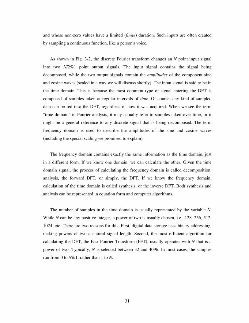
As shown in Fig. 3-2, the discrete Fourier transform changes an N point input signal
into two N/2%1 point output signals. The input signal contains the signal being
decomposed, while the two output signals contain the amplitudes of the component sine
and cosine waves (scaled in a way we will discuss shortly). The input signal is said to be in
the time domain. This is because the most common type of signal entering the DFT is
composed of samples taken at regular intervals of time. Of course, any kind of sampled
data can be fed into the DFT, regardless of how it was acquired. When we see the term
"time domain" in Fourier analysis, it may actually refer to samples taken over time, or it
might be a general reference to any discrete signal that is being decomposed. The term
frequency domain is used to describe the amplitudes of the sine and cosine waves
(including the special scaling we promised to explain).
The frequency domain contains exactly the same information as the time domain, just
in a different form. If we know one domain, we can calculate the other. Given the time
domain signal, the process of calculating the frequency domain is called decomposition,
analysis, the forward DFT, or simply, the DFT. If we know the frequency domain,
calculation of the time domain is called synthesis, or the inverse DFT. Both synthesis and
analysis can be represented in equation form and computer algorithms.
The number of samples in the time domain is usually represented by the variable N.
While N can be any positive integer, a power of two is usually chosen, i.e., 128, 256, 512,
1024, etc. There are two reasons for this. First, digital data storage uses binary addressing,
making powers of two a natural signal length. Second, the most efficient algorithm for
calculating the DFT, the Fast Fourier Transform (FFT), usually operates with N that is a
power of two. Typically, N is selected between 32 and 4096. In most cases, the samples
run from 0 to N&1, rather than 1 to N.

32
Fig. 3-2. DFT terminology. In the time domain, x[ ] consists of N points running from 0
to N&1. In the frequency domain, the DFT produces two signals, the real part, written:
ReX[ ], and the imaginary part, written: Im X[ ]. Each of these frequency domain signals
are N/2%1 points long, and run from 0 to N/2. The Forward DFT transforms from the time
domain to the frequency domain, while the Inverse DFT transforms from the frequency
domain to the time domain. (Take note: this figure describes the real DFT. The complex
DFT, discussed in Chapter 31, changes N complex points into another set of N complex
points).
There are several ways to calculate the Discrete Fourier Transform (DFT), such as
solving simultaneous linear equations or the correlation method. The Fast Fourier
Transform (FFT) is another method for calculating the DFT. While it produces the same
result as the other approaches, it is incredibly more efficient, often reducing the
computation time by hundreds. This is the same improvement as flying in a jet aircraft
versus walking. While the FFT only requires a few dozen lines of code, it is one of the
most complicated algorithms in DSP. But we can easily use published FFT routines
without fully understanding the internal workings.
Figure 3-3 shows the structure of the entire FFT. The time domain decomposition is
accomplished with a bit reversal sorting algorithm. Transforming the decomposed data into
the frequency domain involves nothing and therefore does not appear in the figure. The
frequency domain synthesis requires three loops. The outer loop runs through the Log
stages (i.e., each level in Fig. 3-3, starting from the bottom 2N and moving to the top). The
middle loop moves through each of the individual frequency spectra in the stage being
worked on (i.e., each of the boxes on any one level in Fig. 3-3). The innermost loop uses

33
the butterfly to calculate the points in each frequency spectra (i.e., looping through the
samples inside anyone box in Fig. 3-3). The overhead boxes in Fig. 3-3 determine the
beginning and ending indexes for the loops, as well as calculating the sinusoids needed in
the butterflies.
Fig. 3-3. Flow diagram of the FFT. This is based on three steps: (1) decompose an N point
time domain signal into N signals each containing a single point, (2) find the spectrum of
each of the N point signals (nothing required), and (3) synthesize the N frequency spectra
into a single frequency spectrum.
3.2 Programming models
Parallel programming represents the next turning point in how software engineers write
software. Multicore processors can be found today in the heart of supercomputers, desktop
computers and laptops. Consequently, applications will increasingly need to be parallelized
to fully exploit multicore processors throughput gains now becoming available [Towards
High-Level Parallel Programming Models]. Here we provide an explanation of the main

34
characteristics of some programming models, including OpenMP which is the most
popular and the one we decided to study first.
3.2.1 Pthreads
This is a set of threading interfaces developed by the IEEE (Institute of Electrical and
Electronics Engineers) committees in charge of specifying a Portable Operating System
Interface (POSIX) [7]. It realizes the shared-memory programming model via a collection
of routines for creating, managing and coordinating a collection of threads. Thus, like MPI,
it is a library. Some features were primarily designed for uniprocessors, where context
switching enables a time-sliced execution of multiple threads, but it is also suitable for
programming small shared memory system processors.
The Pthreads library aims to be expressive as well as portable, and it provides a fairly
comprehensive set of features to create, terminate, and synchronize threads and to prevent
different threads from trying to modify the same values at the same time: it includes
mutexes, locks, condition variables, and semaphores. However, programming with
Pthreads is much more complex than with OpenMP, and the resulting code is likely to
differ substantially from a prior sequential program (if there is one). Even simple tasks are
performed via multiple steps, and thus a typical program will contain many calls to the
Pthreads library. For example, to execute a simple loop in parallel, the programmer must
declare threading structures, create and terminate the threads individually, and compute the
loop bounds for each thread. If interactions occur within loop iterations, the amount of
thread-specific code can increase substantially. Compared to Pthreads, the OpenMP API
directives make it easy to specify parallel loop execution, to synchronize threads, and to
specify whether or not data is to be shared. For many applications, this is sufficient. In the
other hand, programming with Pthreads has the advantage that the programmer can control
in a explicit way what and how the parallelism of the application. The following is an
example of a program for creation-termination of threads using Pthreads.
#include <pthread.h>
#include <stdio.h>
#define NUM_THREADS 5

35
void *PrintHello(void *threadid)
{
long tid;
tid = (long)threadid;
printf("Hello World! It's me, thread #%ld!\n", tid);
pthread_exit(NULL);
}
int main (int argc, char *argv[])
{
pthread_t threads[NUM_THREADS];
int rc;
long t;
if (t==0){
printf("There are %d threads\n", NUM_THREADS);
}
pthread_exit(NULL);
}
Example 3-1. Printing hello world and number of threads with Pthreads
While the Pthreads library is fairly comprehensive (although not quite as extensive as
some other native API sets) and distinctly portable, it suffers from a serious limitation
common to all native threading APIs: it requires considerable threading-specific code. In
other words, coding for Pthreads irrevocably casts the codebase into a threaded model.
Moreover, certain decisions, such as the number of threads to use can become hard-coded
into the program. In exchange for these constraints, Pthreads provides extensive control
over threading operations—it is an inherently low-level API that mostly requires multiple
steps to perform simple threading tasks. For example, using a threaded loop to step through
a large data block requires that threading structures be declared, that the threads be created
individually, that the loop bounds for each thread be computed and assigned to the thread,
and ultimately that the thread termination be handled—all this must be coded by the
developer. If the loop does more than simply iterate, the amount of thread-specific code
can increase substantially. To be fair, the need for this much code is true of all native
threading APIs, not just Pthreads.
In a shared-memory architecture all threads have access to the same global, shared
memory. All threads also have their own private data and the programmers are responsible
for synchronizing access (protecting) globally shared data.

36
Fig. 3-4. Threads under a shared memory model architecture.
3.2.2 OpenMP
The OpenMP Application Programming Interface (API) was developed to enable
portable shared memory parallel programming [7]. It aims to support the parallelization of
applications from many disciplines. Moreover, its creators intended to provide an approach
that was relatively easy to learn as well as apply.
The API is designed to permit an incremental approach to parallelizing an existing code,
in which portions of a program are parallelized, possibly in successive steps.
This is a marked contrast to the all-or-nothing conversion of an entire program in a
single step that is typically required by other parallel programming paradigms. It was also
considered highly desirable to enable programmers to work with a single source code: if a
single set of source files contains the code for both the sequential and the parallel versions
of a program, then program maintenance is much simplified. These goals have done much
to give the OpenMP API its current shape.
A thread is a runtime entity that is able to independently execute a stream of
instructions. OpenMP builds on a large body of work that supports the specification of

37
programs for execution by a collection of cooperating threads. The operating system
creates a process to execute a program: it will allocate some resources to that process,
including pages of memory and registers for holding values of objects. If multiple threads
collaborate to execute a program, they will share the resources, including the address space,
of the corresponding process. The individual threads need just a few resources of their own:
a program counter and an area in memory to save variables that are specific to it (including
registers and a stack). Multiple threads may be executed on a single processor or core via
context switches; they may be interleaved via simultaneous multithreading. Threads
running simultaneously on multiple processors or cores may work concurrently to execute
a parallel program.
Multithreaded programs can be written in various ways, some of which permit complex
interactions between threads. OpenMP attempts to provide ease of programming and to
help the user avoid a number of potential programming errors, by offering a structured
approach to multithreaded programming. It supports the so-called fork-join programming
model, which is illustrated in Figure 3.5. Under this approach, the program starts as a
single thread of execution, just like a sequential program. The thread that executes this
code is referred to as the initial thread. Whenever an OpenMP parallel construct is
encountered by a thread while it is executing the program, it creates a team of threads (this
is the fork), becomes the master of the team, and collaborates with the other members of
the team to execute the code dynamically enclosed by the construct. At the end of the
construct, only the original thread, or master of the team, continues; all others terminate
(this is the join). Each portion of code enclosed by a parallel construct is called a parallel
region.
Fig. 3.5. The fork-join model

38
OpenMP expects the application developer to give a high-level specification of the
parallelism in the program and the method for exploiting that parallelism. Thus it provides
notation for indicating the regions of an OpenMP program that should be executed in
parallel; it also enables the provision of additional information on how this is to be
accomplished. The job of the OpenMP implementation is to sort out the low-level details
of actually creating independent threads to execute the code and to assign work to them
according to the strategy specified by the programmer.
It is much easier to make a parallel program with OpenMP directives. Here is the
respective example of a parallel application using OpenMP.
#include <omp.h>
#include <iostream>
int main (int argc, char *argv[]) {
int th_id, nthreads;
#pragma omp parallel private(th_id)
{
th_id = omp_get_thread_num();
printf(“Hello World from thread %d\n", th_id);
#pragma omp barrier
if ( th_id == 0 ) {
nthreads = omp_get_num_threads();
Printf("There are %d threads\n", nthreads);
}
}
return 0;
}
Example 3-2. Printing a hello world and number of Threads with Openmp.
The core elements of OpenMP are the constructs for thread creation, work load distribution
(work sharing), data environment management, thread synchronization, user level runtime
routines and environment variables.

39
Fig. 3-6. Chart of OpenMP Constructs.
We have start our research by adopting OpenMP as a programming model. In the
chapter 4 we will explain the consideration that we need to keep in mind in order to
optimize a parallel OpenMP application.
3.2.3 Cilk
Cilk is an algorithmic multithreaded language [13]. The biggest principle behind the
design of the Cilk language is that the programmer should be responsible for exposing the
parallelism, identifying elements that can safely be executed in parallel; it should then be
left to the run-time environment, particularly the scheduler, to decide during execution how
to actually divide the work between processors. It is because these responsibilities are
separated that a Cilk program can run without rewriting on any number of processors,
including one.
The keyword cilk identifies a Cilk procedure, which is the parallel version of a C function.
A Cilk procedure may spawn subprocedures in parallel and synchronize upon their
completion.
Figure 3-7 show a diagram of that parallel routines division. Each procedure, shown as
a rounded rectangle, is broken into sequences of threads, shown as circles. A downward
edge indicates the spawning of a subprocedure. A horizontal edge indicates the
continuation to a successor thread. An upward edge indicates the returning of a value to a

40
parent procedure. All three types of edges are dependencies which constrain the order in
which threads may be scheduled.
Fig. 3-7.The Cilk model of multithreaded computation.
Fig. 3-8. Cilk components.
The following is an example of an Cilk parallel program. The parallelism is declared at
process level.

41
cilk int fib(n) {
if (n < 2) return n;
else {
int n1, n2;
n1 = spawn fib(n-1);
n2 = spawn fib(n-2);
sync;
return (n1 + n2);
}
}
Example 3-3. Fibonaci numbers calculation with cilk.
3.2.4 The Intel threading building blocks (TBB)
Intel TBB [17] is a library that supports scalable parallel programming using standard
C++ code. It does not require special languages or compilers. The ability to use Threading
Building Blocks on virtually any processor or any operating system with any C++ compiler
makes it very appealing. Threading Building Blocks uses templates for common parallel
iteration patterns, enabling programmers to attain increased speed from multiple processor
cores without having to be experts in synchronization, load balancing, and cache
optimization. Programs using Threading Building Blocks will run on systems with a single
processor core, as well as on systems with multiple processor cores. Threading Building
Blocks promotes scalable data parallel programming. Additionally, it fully supports nested
parallelism, so we can build larger parallel components from smaller parallel components
easily. To use the library, we specify tasks, not threads, and let the library map tasks onto
threads in an efficient manner. The result is that Threading Building Blocks enables us to
specify parallelism far more conveniently, and with better results, than using raw threads.
This library differs from typical threading packages in these ways:
Threading Building Blocks enables us to specify tasks instead of threads: Most
threading packages require us to create, join, and manage threads. Programming directly in
terms of threads can be tedious and can lead to inefficient programs because threads are
low-level, heavy constructs that are close to the hardware. Direct programming with

42
threads forces us to do the work to efficiently map logical tasks onto threads. In contrast,
the Threading Building Benefits Blocks runtime library automatically schedules tasks onto
threads in a way that makes efficient use of processor resources. The runtime is very
effective at load balancing the many tasks we will be specifying.
By avoiding programming in a raw native thread model, we can expect better portability,
easier programming, more understandable source code, and better performance and
scalability in general.
Indeed, the alternative of using raw threads directly would amount to programming
in the assembly language of parallel programming. It may give us maximum
flexibility, but with many costs.
Threading Building Blocks targets threading for performance: Most general-purpose
threading packages support many different kinds of threading, such as threading for
asynchronous events in graphical user interfaces. As a result, general-purpose packages
tend to be low-level tools that provide a foundation, not a solution. Instead, Threading
Building Blocks focuses on the particular goal of parallelizing computationally intensive
work, delivering higher-level, simpler solutions.
Threading Building Blocks is compatible with other threading packages: Threading
Building Blocks can coexist seamlessly with other threading packages. This is very
important because it does not force us to pick among Threading Building Blocks, OpenMP,
or raw threads for our entire program. We are free to add Threading Building Blocks to
programs that have threading in them already. We can also add an OpenMP directive, for
instance, somewhere else in our program that uses Threading Building Blocks. For a
particular part of our program, we will use one method, but in a large program, it is
reasonable to anticipate the convenience of mixing various techniques. It is fortunate that
Threading Building Blocks supports this.
.
Threading Building Blocks emphasizes scalable, data-parallel programming:
Breaking a program into separate functional blocks and assigning a separate thread to each

43
block is a solution that usually does not scale well because, typically, the number of
functional blocks is fixed. In contrast, Threading Building Blocks emphasizes data-
parallel programming, enabling multiple threads to work most efficiently together. Data-
parallel programming scales well to larger numbers of processors by dividing a data set
into smaller pieces. With data parallel programming, program performance increases
(scales) as we add processors. Threading Building Blocks also avoids classic bottlenecks,
such as a global task queue that each processor must wait for and lock in order to get a new
task.
Threading Building Blocks relies on generic programming: Traditional libraries specify
interfaces in terms of specific types or base classes. Instead, Threading Building Blocks
uses generic programming, which is defined in Chapter 12. The essence of generic
programming is to write the best possible algorithms with the fewest constraints. The C++
Standard Template Library (STL) is a good example of generic programming in which the
interfaces are specified by requirements on types.
For example, C++ STL has a template function that sorts a sequence abstractly, defined in
terms of iterators on the sequence. Generic programming enables Threading Building
Blocks to be flexible yet efficient. The generic interfaces enable us to customize
components to our specific needs.
TBB vs OpenMP
OpenMP has the programmer choose among three scheduling approaches (static,
guided, and dynamic) for scheduling loop iterations. Threading Building Blocks does not
require the programmer to worry about scheduling policies. Threading Building Blocks
does away with this in favor of a single, automatic, divide-and-conquer approach to
scheduling. Implemented with work stealing (a technique for moving tasks from loaded
processors to idle ones), it compares favorably to dynamic or guided scheduling, but
without the problems of a centralized dealer. Static scheduling is sometimes faster on

44
systems undisturbed by other processes or concurrent sibling code. However, divide-and-
conquer comes close enough and fits well with nested parallelism.
The generic programming embraced by Threading Building Blocks means that
parallelism structures are not limited to built-in types. OpenMP allows reductions on only
built-in types, whereas the Threading Building Blocks parallel_reduce works on any type.
Looking to address weaknesses in OpenMP, Threading Building Blocks is designed for
C++, and thus to provide the simplest possible solutions for the types of programs written
in C++. Hence, Threading Building Blocks is not limited to statically scoped loop nests.
Far from it: Threading Building Blocks implements a subtle but critical recursive model of
task-based parallelism and generic algorithms.
3.2.5 Java Threads
In contrast to most other programming languages where the operating system and a
specific thread library like Pthreads [18] or C-Threads are responsible for the thread
management, Java [Efficiency of Thread-parallel Java Programs from Scientific Computing] has a
direct support for multithreading integrated in the language. The java.lang package
contains a thread API consisting of the class Thread and the interface Runnable. There are
two basic methods to create threads in Java. Figure 3-9 shows the life cycle of a java thread.
Fig. 3-9. Life Cycle of Java Threads

45
The states of a java thread are the following:
New Thread: When a thread is in the "New Thread" state, it is an empty Thread object.
The run() is not being run and the processor time is not allocated. In order to start the
thread one must invoke the start() method. In this state it is also possible to invoke the
stop() method, which will kill the thread. Calling any method besides start() or stop() when
a thread is in this state causes an IllegalThreadStateException.
Runnable: A thread is in this state after the start() method calls the thread's run() method.
At this point the thread is in the "Runnable" state. This state is called "Runnable" rather
than "Running" because the thread might not actually be running when it is in this state.
The "Running" state is a sub-state of the "Runnable" state and a thread is in the "Running"
state when the scheduling mechanism gives up the CPU time to the thread, for example
when the yield() is invoked. So, the Java runtime system must implement a scheduling
scheme that shares the processor between all "Runnable" threads.
Non Runnable: A thread enters the "Not Runnable" state when one of the following
events occurs:
• The thread invokes its sleep() method.
• Some other thread invokes the sleep() method of the current thread.
• The thread invokes its suspend() method.
• Some other thread invokes the suspend() method of the current thread.
• The thread uses its wait() method to wait on a condition variable.
• The thread is blocking on I/O.
For each of the entrances into the "Not Runnable" state shown in the figure, there is
a specific and distinct transition of the thread to the "Runnable" state.
The following indicates the transitions for every entrance into the "Not Runnable"
state.
• If a thread has been transfered in the "Non Runnable" state by the sleep(),
then the specified number of milliseconds must elapse.

46
• If a thread has been transfered in the "Non Runnable" state by the suspend(),
then someone must call its resume() method.
• If a thread is waiting on a condition variable, whatever object owns the
variable must relinquish it by calling either notify() or notifyAll().
• If a thread is blocked on I/O, then the I/O must complete.
Dead
A thread can die in two ways: when its run() method exits normally, or being killed
(stopped), invoking the stop() method.
Threads can be generated by specifying a new class which inherits from Thread and by
overriding the run() method in the new class with the code that should be executed by the
new thread. A new thread is then related by generating an object of the new class and
calling its start() method.
An alternative way to generate threads is by using the interface Runnable which
contains only the abstract method run(). The Thread class actually implements the
Runnable interface and, thus, a class inheriting from Thread also implements the Runnable
interface.
The creation of a thread without inheriting from the Thread class consists of two steps:
At first, a new class is specified which implements the Runnable interface and overrides
the run() method with the code that should be executed by the thread. After that, an object
of the new class is generated and is passed as an argument to the constructor method of the
Thread class. The new thread is then started by calling the start() method of the Thread
object. A thread is terminated if the last statement of the run() method has been executed.
An alternative way is to call the interrupt() method of the corresponding Thread object.
The method setPriority(int prio) of the Thread class can be used to assign a priority level
between 1 and 10 to a thread where 10 is the highest priority level. The priority of a thread
is used for the scheduling of the user level threads by the thread library.

47
4 Performance analysis and Tuning
Our research aims to provide a guide of what are the good practices we must have into
account when analyzing and tuning an OpenMP parallel application. Also we provide an
explanation of the tools used to analyze the execution performance of those applications. In
the future we aim to extent this guide to a performance model for multithread application
programmed under other programming models. This research provides a set of key factor
to have in mind when parallelizing a multithread application.
In order to find the reasons of a poor performance, it is necessary to understand how
the application is organized. As we said in the introduction to this master thesis, we haven`t
followed the general model where the analysis of the application is done taking the
application as a black box. Our work differs from the general model in that, doing the
analysis on that way might be sometimes more difficult due to the lack of knowledge of the
application’s task flow. Therefore we have gone one step ahead in the analysis of the
applications through extraction the applications structure and execution patterns.
4.1 Key factors to improve the performance
Here we explain what issues we must have into account when we analyze the
performance and tune multithread applications. The key attributes that affect parallel
performance are coverage, granularity, load balancing, locality, and synchronization. The
first three are fundamental to parallel programming on any type of machine. However
locality is a very important issued to have in mind when optimizing a multithread
application in a shared memory system. Their effects are often more surprising and harder
to understand, and their impact can be huge.
4.1.1 Coverage and Granularity
In order to get good performance on a parallel code, it is necessary to parallelize a
sufficiently large portion of the code [19]. This is a fairly obvious concept, but what is less
obvious and what is perhaps even counterintuitive is that as the number of processors is
increased, the performance of the application can become dominated by the serial portions
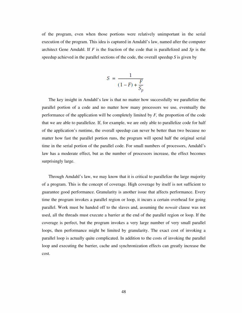
48
of the program, even when those portions were relatively unimportant in the serial
execution of the program. This idea is captured in Amdahl’s law, named after the computer
architect Gene Amdahl. If F is the fraction of the code that is parallelized and Sp is the
speedup achieved in the parallel sections of the code, the overall speedup S is given by
The key insight in Amdahl’s law is that no matter how successfully we parallelize the
parallel portion of a code and no matter how many processors we use, eventually the
performance of the application will be completely limited by F, the proportion of the code
that we are able to parallelize. If, for example, we are only able to parallelize code for half
of the application’s runtime, the overall speedup can never be better than two because no
matter how fast the parallel portion runs, the program will spend half the original serial
time in the serial portion of the parallel code. For small numbers of processors, Amdahl’s
law has a moderate effect, but as the number of processors increase, the effect becomes
surprisingly large.
Through Amdahl’s law, we may know that it is critical to parallelize the large majority
of a program. This is the concept of coverage. High coverage by itself is not sufficient to
guarantee good performance. Granularity is another issue that affects performance. Every
time the program invokes a parallel region or loop, it incurs a certain overhead for going
parallel. Work must be handed off to the slaves and, assuming the nowait clause was not
used, all the threads must execute a barrier at the end of the parallel region or loop. If the
coverage is perfect, but the program invokes a very large number of very small parallel
loops, then performance might be limited by granularity. The exact cost of invoking a
parallel loop is actually quite complicated. In addition to the costs of invoking the parallel
loop and executing the barrier, cache and synchronization effects can greatly increase the
cost.

49
4.1.2 Synchronization
Another key performance factor is synchronization. We will consider two types of
synchronization: barriers and mutual exclusion.
Barriers
Barriers are used as a global point of synchronization. A typical use of barriers is at the end
of every parallel loop or region. This allows the user to consider a parallel region as an
isolated unit and not have to consider dependences between one parallel region and another
or between one parallel region and the serial code that comes before or after the parallel
region. Barriers are very convenient, but on a machine without special support for them,
barriers can be very expensive [22].
Implicit barriers are put at the end of all work-sharing constructs. The user can avoid
these barriers by use of the nowait clause. This allows all threads to continue processing at
the end of a work-sharing construct without having to wait for all the threads to complete.
Of course, the user must insure that it is safe to eliminate the barrier in this case. Another
technique to avoiding barriers is to combine multiple parallel loops into one.
If two loops have dependency of each other, it is not recommended to run both
separately in parallel. Example 4-1 shows a code with adjacent parallel loops.
#pragma omp for for(i=0; i< N; i++){
a(i) = ... } #pragma omp for for(i=0; i< N; i++){
b(i) = a(i) + ... }
Example 4-1. Code with multiple adjacent parallel loops
There is a dependency between the two loops, so we cannot simply run the two loops in
parallel with each other, but the dependence is only within corresponding iterations.
Iteration i of the second loop cannot proceed until iteration i of the first loop is finished,
but all other iterations of the second loop do not depend on iteration i. We can eliminate an

50
implicit barrier (and also the overhead cost for starting a parallel loop) by fusing the two
loops together as follows in Example 4-2.
#pragma omp for for(i=0; i< N; i++){
a(i) = ... b(i) = a(i) + ...
}
Example 4-2. Code with multiple adjacent parallel loops
4.1.3 Memory access patterns
Memory access patterns is consider by many researchers the most important factor
when we an application is running in a multicore environment [7]. A modern memory
system is organized as a hierarchy, where the largest, and also slowest, part of memory is
known as main memory. Main memory is organized into pages (physical and virtual); a
subset of it will be available to a given application. The memory levels closer to the
processor are successively smaller and faster and are collectively known as cache. When a
program is compiled, the compiler will arrange for its data objects to be stored in main
memory; they will be transferred to cache when needed. If a date is required for a
computation is not already in a cache (we call this a cache “miss”), it must be retrieved
from higher levels of the memory hierarchy, a process that can be quite expensive.
Program data is brought into cache in chunks called blocks, each of which will occupy a
line of cache. Data that is already in cache may need to be replaced, to make space for a
new block of data. Different systems have different strategies for deciding what must go.
The memory hierarchy is (with rare exceptions) not explicitly programmable by either
the user or the compiler. Rather, data are fetched into cache and evicted from it
dynamically as the need arises. Given the penalty paid whenever values must be retrieved
from other levels of memory, various strategies have been devised that can help the
compiler and the programmer to (indirectly) reduce the frequency with which this situation
occurs.
The first thing a programmer must have into account in order to avoid data cache
misses is to organize data accesses. In that way the different elements of data will be used

51
as often as possible during the time they are stored in the cache. One strategy is the most
common languages like C or Fortran, typically store in cache memory the neighbor
elements.
So far in our research we have analyzed scientific applications programmed in C or
C++. These languages specifies for example that a two dimensional array will be stored in
rows. The elements nearby to the stored element will be stored too as part of the language
strategy. Figure 4-1 shows an example, in a two dimensional array, if the element [0][2] is
stored in memory, also the elements [0][1] and [0][3] will be stored. This strategy is known
as “rowwise”. For a good performance, in a matrix-based computation the elements most
be accessed by rows and not by columns.
[0][0] [0][1] [0][2] [0][3]
First storedElement
NearbyElements
[0][4]
Fig. 4-1. Strategy to store elements in the cache memory
A programmer must be sure to access the array by rows and not by columns. The following
are two examples of correct and incorrect accesses respectively.
for (i=0; i<N; i++){
for (j=0; j<N; j++){
sum += a[i][j];
Example 4-1: Correct access, the array a is accessed by along the rows. On this way we
can assure a good performance regarding memory system. This type of access is known as
unit stride.
for (j=0; j<N; j++){
for (i=0; i<N; i++){

52
sum += a[i][j];
Example 4-2: Incorrect access, this type of access is called columnwise. It is not friendly
to the applications performance. As long as the array grows, the performance will get
worse.
4.1.4 Inconsistent parallelization
Another situation that can lead to locality problems is inconsistent parallelization [19].
Imagine the following set of two loops:
for (i=0; i<N,i++) {
a(i) = b(i) } for (i=0; i<N,i++) {
a(i) = a(i) + a(i – 1) }
Example 4-3. Example of inconsistent parallelism in loops
The first loop can be trivially parallelized. The second loop cannot easily be
parallelized because every iteration depends on the value of a(i–1) written in the previous
iteration. We might have a tendency to parallelize the first loop and leave the second one
sequential. But if the arrays are small enough to fit in the aggregate caches of the
processors, this can be the wrong decision. By parallelizing the first loop, we have divided
the a matrix among the caches of the different processors. Now the serial loop starts and all
the data must be brought back into the cache of the master processor. As we have seen, this
is potentially very expensive, and it might therefore have been better to let the first loop
run serially.
4.1.5 Loop optimization
Since many programs spend much of their time executing loops and since most array
accesses are to be found there, a suitable reorganization of the computation in loop nests to
exploit cache can significantly improve a program’s performance [7]. A number of loop
transformations can help achieve this. They can be applied if the changes to the code do
not affect correct execution of the program. The test for this is as follows:

53
If any memory location is referenced more than once in the loop nest and if at least one of
those references modifies its value, then their relative ordering must not be changed by the
transformation.
A programmer should consider transforming a loop if accesses to arrays in the loop nest do
not occur in the order in which they are stored in memory, or if a loop has a large body and
the references to an array element or its neighbors are far apart[].
Loop interchange: If we encounter that a array is being accessed through a columnwise
pattern in a C/C++ piece of code we must exchange the loop headers in order to change the
access pattern to rowwise. This is what we call loop interchange.
Loop unrolling: This technique is about do more with less resources, the loop in the
example 4-3 loads four array elements (b[i], a[i], a[a-1], b[i-1]), performs three floating-
point additions, and stores two values per iteration. The overhead of that loops is generated
when the loop variable is incremented, when the value is tested and when it performs a
branch to the start of the loop.
for (int i=1; i<n; i++) { a[i] = b[i] + 1; c[i] = a[i] + a[i-1] + b[i-1];
}
Example 4-3: A short loop nest – Loop overheads are relatively high when each iteration
has a small number of operations.
The whole overhead of the loop in the example 4-3 can be halved by unrolling the loop
to get another one as shown in the example 4-4. This loop loads five elements ( b[i], b[i-1],
b[i+1], a[i] , carries out six floating-point additions and stores four values with the same
overhead. The data reuse has improved, too. When one is updating c[i+1], the value of a[i]
just computed can be used immediately. There is no risk that the reference to a[i] might
force new data to be brought into cache. The newly computed value is still in a register and
hence available for use. When one is updating c[i+1], the value of a[i] just computed can
be used immediately. There is no risk that the reference to a[i] might force new data to be

54
brought into cache. The newly computed value is still in a register and hence available for
use.
In this example, the loop body executes 2 iterations in one pass. This number is called the
“unroll factor.” The appropriate choice depends on various constraints. A higher value
tends to give better performance but also increases the number of registers needed, for
example.
for (int i=1; i<n; i+=2) {
a[i] = b[i] + 1; c[i] = a[i] + a[i-1] + b[i-1]; a[i+1] = b[i+1] + 1; c[i+1] = a[i+1] + a[i] + b[i];
}
Example 4-4. A loop with an unroll factor of two.
Unroll and jam is an extension of loop unrolling that is appropriate for some loop nests
with multiple loops. When two loops that are tightly nested, as shown in the example 4-.5,
and there are few operation inside a nested loop, the nest loop had better to be unroll.
for (int j=0; j<n; j++) for (int i=0; i<n; i++)
a[i][j] = b[i][j] + 1;
Example 4-5. A loop that does not benefit from inner loop unrolling. In this case, unrolling
the loop over i results in poor cache utilization. It is assumed the iteration count is divisible
by two.
This loop nest is a prime candidate for unrolling because there is not much computation
per iteration. Unfortunately, unrolling the inner loop over i results in strode access to
elements of arrays a and b. If, however, we unroll the outer loop, as in the example 4-6,
then we have the desired rowwise array access.
for (int j=0; j<n; j+=2){ for (int i=0; i<n; i++)
a[i][j] = b[i][j] + 1; for (int i=0; i<n; i++)
a[i][j+1] = b[i][j+1] + 1; }

55
Example 4-6. Another example of a loop with an unroll factor of two.
4.1.6 Dynamic threads
So far we have considered the performance impact of how the programmer code and
parallelize the algorithm, but we have considered the program as an isolated unit. There
has been no discussion of how the program interacts with other programs in a computer
system. In some environments, we might have the entire computer system to ourselves. No
other application will run at the same time as ours. Or, we might be using a batch scheduler
that will insure that every application runs separately, in turn. In either of these cases, it
might be perfectly reasonable to look at the performance of our program in isolation. On
some systems and at sometimes, though, we might be running in a multiprogramming
environment. Some set of other applications might be running concurrently with our
application. The environment might even change throughout the execution time of our
program. Some other programs might start to run, others might finish running, and still
others might change the number of processors that are being used.
OpenMP allows two different execution models. In one model, the user specifies the
number of threads, and the system gives the user exactly that number of threads. If there
are not enough processors or there are not enough free processors, the system might choose
to multiplex those threads over a smaller number of processors, but from the program’s
point of view the number of threads is constant. So, for example, in this mode running the
following code fragment:
omp_set_num_threads(4) #pragma omp parallel { #pragma omp critical
{ print *, 'Hello' }
}
Example 4-7. A parallel region with one critical region
It will always print “Hello” four times, regardless of how many processors are available. In
the second mode, called dynamic threads [19], the system is free at each parallel region or

56
parallel do to lower the number of threads. With dynamic threads, running the above code
might result in anywhere from one to four “Hello”s being printed. Whether or not the
system uses dynamic threads is controlled either via the environment variable
OMP_DYNAMIC or the runtime call omp_set_dynamic. The default behavior is
implementation dependent.
If the program relies on the exact number of threads remaining constant, if, for example,
it is important that “Hello” is printed exactly four times, dynamic threads cannot be used. If,
on the other hand, the code does not depend on the exact number of threads, dynamic
threads can greatly improve performance when running in a multiprogramming
environment (dynamic threads should have minimal impact when running stand-alone or
under batch systems).
Why performance improves using dynamic threads? To understand, let’s first consider the
simple example of trying to run a three-thread job on a system with only two processors.
The system will need to multiplex the jobs among the different processors. Every so often,
the system will have to stop one thread from executing and give the processor to another
thread. Imagine, for example, that the stopped, or preempted, thread was in the middle of
executing a critical section. Neither of the other two threads will be able to proceed. They
both need to wait for the first thread to finish the critical section. If we are lucky, the
operating system might realize that the threads are waiting on a critical section and might
immediately preempt the waiting threads in favor of the previously preempted thread.
More than likely, however, the operating system will not know, and it will let the other two
threads spin for a while waiting for the critical section to be released. Only after a fixed
time interval will some thread get preempted, allowing the holder of the critical section to
complete. The entire time interval is wasted.
One might argue that the above is an implementation weakness. The OpenMP system
should communicate with the operating system and inform it that the other two threads are
waiting for a critical section. The problem is that communicating with the operating system
is expensive. The system would have to do an expensive communication every critical
section to improve the performance in the unlikely case that a thread is preempted at the

57
wrong time. One might also argue that this is a degenerate case: critical sections are not
that common, and the likelihood of a thread being preempted at exactly the wrong time is
very small. Perhaps that is true, but barriers are significantly more common. If the duration
of a parallel loop is smaller than the interval used by the operating system to multiplex
threads, it is likely that at every parallel loop the program will get stuck waiting for a
thread that is currently preempted.
4.2 Performance Analysis tools evaluated
The study of performance evaluation as an independent subject has sometimes caused
researchers in the area to lose contact with reality” [14]. It is important to ask why is it that
performance evaluation is by no means an integrated and natural part of software
development?. The following are some realities that answer the previous question.
• The primary duty of software developers is to create functionally correct programs.
• Performance evaluation tends to be optional.
• “Contrary to common belief, performance evaluation is an art. ... Like artist, each
analyst has a unique style. Given the sample problem, two analysts may choose
different performance metrics and evaluation methodologies.”, but even they need
tools [].
Performance analysis and tuning of an application as a black box, may only contribute
to achieve a better performance, but not necessarily the best one. It doesn’t free the system
from the overhead produced by an incorrect optimization of the application structure in the
source code. Figure 4-2 shows the flow of a performance optimization cycle of a
application in general.
So far in our research we have tested different tools for performance analysis of
OpenMP applications. From that pursue we have adopted two important tools that offer the
possibility to work together. We offer an explanation of how they work.

58
Fig. 4-2. Performance optimization cycle [14]
4.2.1 PAPI
PAPI aims to provide the tool designer and application engineer with a consistent
interface and methodology for use of the performance counter hardware found in most
major microprocessors [24]. PAPI enables software engineers to see, in near real time, the
relation between software performance and processor events. HW performance counters
provide application developers with valuable information about code sections that can be
improved
Hardware performance counters can provide insight into:
• Whole program timing
• Cache behaviors
• Branch behaviors
• Memory and resource contention and access patterns
• Pipeline stalls

59
• Floating point efficiency
• Instructions per cycle
• Subroutine resolution
• Process or thread attribution
We have implemented the performance analysis dividing it into measurements categories:
• Efficiency o Instructions per cycle (IPC) o Memory bandwidth
• Caches o Data cache misses and miss ratio o Instruction cache misses and miss ratio
• L2 cache misses and miss ratio
• Translation lookaside buffers (TLB) o Data TLB misses and miss ratio o Instruction TLB misses and miss ratio
• Control transfers o Branch mispredictions
Table 4-1. Measurements categories with hardware counters.
For our research we counted with the following list of PAPI hardware counters.
Name Description (Note)
PAPI_L1_DCM Level 1 data cache misses
PAPI_L1_ICM Level 1 instruction cache misses
PAPI_L2_DCM Level 2 data cache misses
PAPI_L2_ICM Level 2 instruction cache misses
PAPI_L1_TCM Level 1 cache misses
PAPI_L2_TCM Level 2 cache misses
PAPI_TLB_DM Data translation lookaside buffer misses
PAPI_TLB_IM Instruction translation lookaside buffer misses

60
PAPI_L1_LDM Level 1 load misses
PAPI_L1_STM Level 1 store misses
PAPI_L2_LDM Level 2 load misses
PAPI_L2_STM Level 2 store misses
PAPI_HW_INT Hardware interrupts
PAPI_BR_CN Conditional branch instructions
PAPI_BR_TKN Conditional branch instructions taken
PAPI_BR_NTK Conditional branch instructions not taken
PAPI_TOT_IIS Instructions issued
PAPI_TOT_INS Instructions completed
PAPI_FP_INS Floating point instructions
PAPI_BR_INS Branch instructions
PAPI_VEC_INS Vector/SIMD instructions
PAPI_RES_STL Cycles stalled on any resource
PAPI_TOT_CYC Total cycles
PAPI_L1_DCH Level 1 data cache hits
PAPI_L1_DCA Level 1 data cache accesses
PAPI_L2_DCA Level 2 data cache accesses
PAPI_L2_DCR Level 2 data cache reads
PAPI_L2_DCW Level 2 data cache writes
PAPI_L1_ICH Level 1 instruction cache hits
PAPI_L2_ICH Level 2 instruction cache hits
PAPI_L1_ICA Level 1 instruction cache accesses
PAPI_L2_ICA Level 2 instruction cache accesses

61
PAPI_L2_TCH Level 2 total cache hits
PAPI_L1_TCA Level 1 total cache accesses
PAPI_L2_TCA Level 2 total cache accesses
PAPI_L2_TCR Level 2 total cache reads
PAPI_L2_TCW Level 2 total cache writes
PAPI_FML_INS Floating point multiply instructions
PAPI_FDV_INS Floating point divide instructions
PAPI_FP_OPS Floating point operations
4.2.2 OMPP
OMPP is a profiling tool for OpenMP applications written in C/C++ or FORTRAN.
ompP’s profiling report becomes available immediately after program termination in a
human-readable format. ompP supports the measurement of hardware performance
counters using PAPI [1] and supports several advanced productivity features such as
overhead analysis and detection of common inefficiency situations (performance
properties).
Instrumenting and Linking Applications with ompP
ompP is implemented as a static library that is linked to our applications. To capture
OpenMP execution events, ompP relies on Opari performance analysis tool for source-to-
source instrumentation. A helper script kinst-ompp or kinst-ompp-papi is included that
hides the details of invoking Opari from the user. To instrument our application with Opari
and link it with ompP’s monitoring library simply prefix any compile or link command
with kinst-ompp or kinst-ompp-papi. I.e., on a shell prompt:
$> gcc -fopenmp nbody.c nbody -o myapp
Becomes
$> kinst-ompp icc -openmp foo.c bar.c -o myapp

62
It is necessary to configure the tool before the installation. We proceeded to modify the
file called makefiles.defs in order to specify the type of c/c++ compiler (CC=gcc), PAPI
library, OpenMP flag (-fopenmp). Similarly, to use ompP with Makefiles, simply replace
the compiler specification like CC=gcc with CC=kinst- mpp gcc.
OMPP recognizes the parallel regions when it founds a OpenMP pragma. It is also
possible for the user to defined his own parallel regions by #pragma pomp inst
begin(function name) at the beginning and #pragma pomp inst end(function name). The
following is an example an user defined region.
Int calculate forces () { #pragma pomp inst begin(foo) //here is the function code #pragma pomp inst end(foo) return 1; }
The following are an example of a simple OpenMP application before and after being
instrumented with OMPP:
Example. 4-8. A simple OpenMP application before being instrumented with OMPP
#include <omp.h>#include <stdio.h>
int main( int argc, char* argv[] ){#pragma omp parallel { int tid; tid = omp_get_thread_num();
fprintf(stderr, "Thread %d of %d\n", tid, omp_get_num_threads() );
} }

63
#ifdef _POMP# undef _POMP#endif#define _POMP 200110
#include "c_simple.c.opari.inc"#line 1 "c_simple.c"
#include <stdio.h>
int main( int argc, char* argv[] ){POMP_Parallel_fork(&omp_rd_2);#line 7 "c_simple.c"#pragma omp parallel POMP_DLIST_00002{ POMP_Parallel_begin(&omp_rd_2);#line 8 "c_simple.c" { int tid; tid = omp_get_thread_num();
fprintf(stderr, "Thread %d of %d\n", tid, omp_get_num_threads() );
}POMP_Barrier_enter(&omp_rd_2);#pragma omp barrierPOMP_Barrier_exit(&omp_rd_2);POMP_Parallel_end(&omp_rd_2); }POMP_Parallel_join(&omp_rd_2);#line 15 "c_simple.c" }
Example. 4-9. A simple OpenMP application after being instrumented with OMPP
OMPP produces a profiling report or trace of file reports during time intervals. The
information is organized into categories. The following is an explanation of those areas.
OmpP Flat Region Profile

64
This section lists flat profiles for each OpenMP construct in a per-region basis. The profiles
in this section are flat. I.e., the times and counts reported are those incurred for the
particular construct, irrespective of how the construct was executed.
Components:
• Region number
• Source code location and region type
• Timing data and execution counts, depending on the particular construct
• One line per thread, last line sums over all threads
• Hardware counter data (if PAPI is available and HW counters are selected)
• Data is exact (measured, not based on sampling)
Call graphs
The data displayed in this section is largely similar to the flat region profiles. However, the
data displayed represents the summed execution times and counts only of the current
execution graph. The path of the root of the callgraph to the current region is shown as the
first lines for each region. The lines have the format [sxy], where xy denotes the level in
the hierarchy, starting with 0 (the root) and the symbol s has the following meaning: *
stands for root of the callgraph + denotes that this entry has children in the call-graph,
while = denotes that this region has no child entries in the callgraph (it is a leaf of the
callgraph). The data entries displayed for callgraph region profiles are similar to the ones
shown for flat profiles. However, for selected columns both inclusive and exclusive data
entries are displayed. Inclusive data represents this region and all descendants, while
exclusive data excludes any descendants. In the example shown above the data is displayed
for a leaf node and hence inclusive and exclusive times for bodyT are the same. Hardware
counter data is handled similar to timing data, i.e., a /I or a /E is appended to the counter
name, for example PAPI_L2_DCM/I and PAPI_L2_DCM/E.
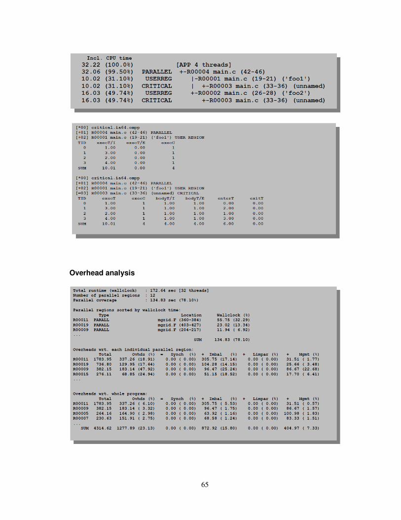
65
Overhead analysis

66
Performance Properties
This section reports so-called “performance properties” that are detected automatically
for the application. Performance properties capture common situations of inefficient
execution, they are based on the profiling data that is reported for each region. Properties
have a name (ImbalanceInParallelLoop) and a context for which they have been detected
(LOOP muldoe.F (68-102)). Each property carries a severity value, which represents the
negative impact on overall performance a property exhibits. The severity value is given in
percentage of total accumulated execution.
Using Hardware Counters with ompP Hardware counters can be used with ompP by setting the environment variables OMPP
CTRn to the names of PAPI predefined or platform-specific event names.
For example:
$> export OMPP_CTR1=PAPI_L2_DCM
The number of hardware counters that can be recorded simultaneously by ompP is a
compile time constant set to 4 per default, see the definition of OMPP PAPI MAX CTRS
in file ompp.h if we want to increase this limit. During startup ompP will display a
message whether registering the specified counter(s)
was successful:
ompP: successfully registered counter PAPI_L2_DCM
If the specified event name(s) are either not recognized or cannot be counted together,
ompP will issue a warning:

67
ompP: PAPI name-to-code error
for an unrecognized event name, or:
ompP: Error adding event to eventset

68
5 Experiments
In any performance analysis system the goal is to understand the behavior of the
application in order to improve it and determine the desired performance [21]. The process
of understand the application behavior and understand the causes of the performance
limitations normally take us to a second stage where we must analyze the source code.
In this chapter explain a set of experiments performed in order to put in practice the
measurements required to achieve a better performance on OpenMP applications. Each
experiment is composed of two parts, methodology and results. The methodology explains
how each experiment was performed as well as other important details. The result part
contains graphical information and its explanation.
5.1 Hardware configuration
The experiments where performed in a homogeneous Intel(R) Xeon(R) model 15 with two
dual-core processors. The following the detail information generated with the command
cpu_info for one the four recognized cores. L2 cache memory is 4MB size, shared by each
pair of core, it is, one L2 memory for each dual core processor.
vendor_id GenuineIntel
cpu family 6
model 15
model name Intel(R) Xeon(R) CPU 5160 @ 3.00GHz
stepping 11
cpu MHz 1992.000
cache size 4096 KB
siblings 2
core id 0
cpu cores 2
Fpu Yes
fpu_exception Yes
cpuid level 10
wp Yes
bogomips 5990.08
clflush size 64
cache_alignment 64
address sizes 38 bits physical, 48 bits virtual

69
Each core has private level 1 cache and shared level 2 cache. The following is detailed
information obtained with the comment papi_mem_info.
Test case: Memory Information.
------------------------------------------------------------------------
L1 Instruction TLB: Number of Entries: 128; Associativity: 4
L1 Data TLB: Number of Entries: 256; Associativity: 4
L1 Instruction Cache
Total size 32KB
Line size 64B
Number of Lines 512
Associativity 8
L1 Data Cache
Total size 32KB
Line size 64B
Number of Lines 512
Associativity 8
L2 Unified Cache
Total size 128KB
Line size 64B
Number of Lines 2048
Associativity 4
L3 Unified Cache
Total size 4096KB
Line size 64B
Number of Lines 65536
Associativity 16
5.2 First group of experiment: Importance of application parallel structure
The objective of the experiment is to demonstrate the importance of the analysis of the
application’s parallel structure to achieve a good performance. Here we use the scientific
application called NBody. There are different algorithms of the NBody-problem, here we
use an implementation called particle-to-particle (see chapter 3).
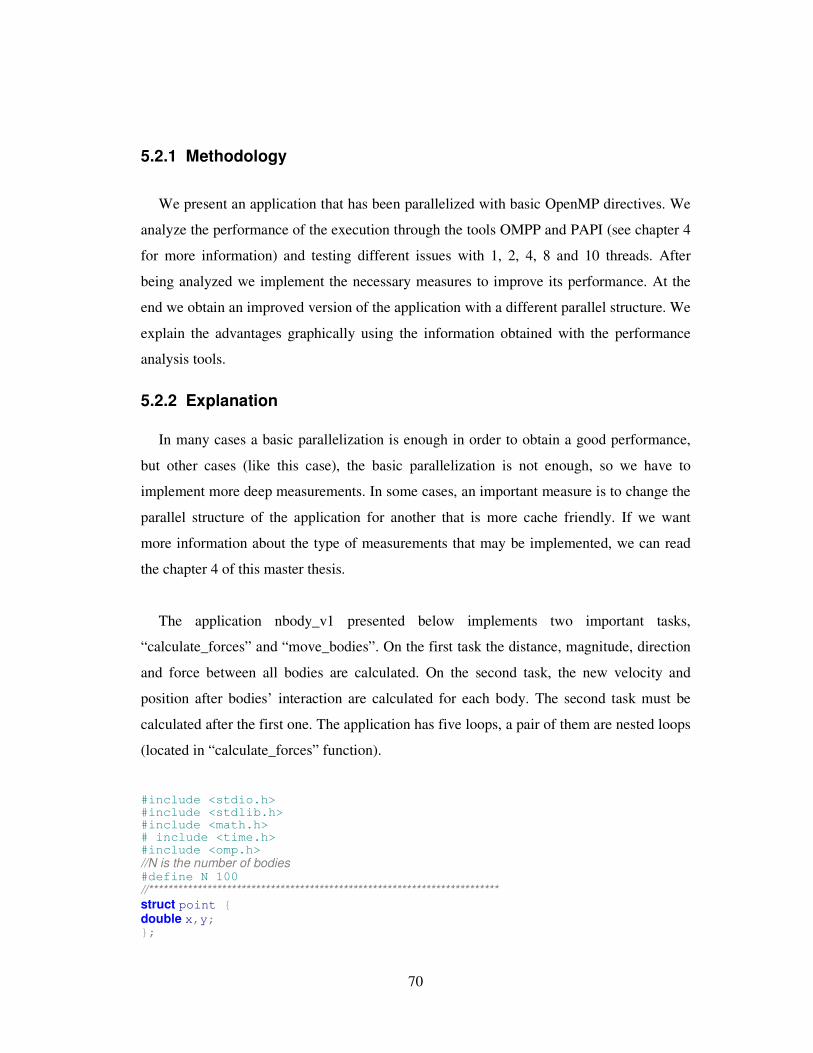
70
5.2.1 Methodology
We present an application that has been parallelized with basic OpenMP directives. We
analyze the performance of the execution through the tools OMPP and PAPI (see chapter 4
for more information) and testing different issues with 1, 2, 4, 8 and 10 threads. After
being analyzed we implement the necessary measures to improve its performance. At the
end we obtain an improved version of the application with a different parallel structure. We
explain the advantages graphically using the information obtained with the performance
analysis tools.
5.2.2 Explanation
In many cases a basic parallelization is enough in order to obtain a good performance,
but other cases (like this case), the basic parallelization is not enough, so we have to
implement more deep measurements. In some cases, an important measure is to change the
parallel structure of the application for another that is more cache friendly. If we want
more information about the type of measurements that may be implemented, we can read
the chapter 4 of this master thesis.
The application nbody_v1 presented below implements two important tasks,
“calculate_forces” and “move_bodies”. On the first task the distance, magnitude, direction
and force between all bodies are calculated. On the second task, the new velocity and
position after bodies’ interaction are calculated for each body. The second task must be
calculated after the first one. The application has five loops, a pair of them are nested loops
(located in “calculate_forces” function).
#include <stdio.h> #include <stdlib.h> #include <math.h> # include <time.h> #include <omp.h>
//N is the number of bodies #define N 100
//************************************************************************ struct point { double x,y; };

71
const double G = 6.67e-11; const double DT = 1.0; // sampling/calculation interval in seconds const double Simulation_Time = 24*60*60; //a day, e.g. struct point p[N],v[N],f[N]; // position force and velocity of each body 0..n double m[N]; // mass of each body 0..n char GCU[10]; //****************************************************************************** ***********************************Function Calculate_forces******************* void calculate_forces() { double distance, magnitude; struct point direction; int i,j; int tid; int thread_num; #pragma omp parallel { #pragma omp for
for (i=0;i<N-1;i++) // for each body except the last one ; for (j=i+1;j<N;j++) { // for each of the rest of the bodies distance = sqrt(pow(p[i].x-p[j].x,2)+pow(p[i].y-p[j].y,2));
magnitude = G * m[i]*m[j] / pow(distance,2); // direction.x = p[j].x-p[i].x; direction.y = p[j].y-p[i].y;
// add the forces to the sum of forces acting on both bodies // watch the signs because the forces are vectors, and act in opposite directions // on i and j #pragma omp critical { f[i].x += magnitude*direction.x/distance; f[j].x -= magnitude*direction.x/distance; f[i].y += magnitude*direction.y/distance; f[j].y -= magnitude*direction.y/distance; }
} } }
//***********************************Function move_bodies*************************** void move_bodies() { struct point deltav; // velocity change: dv = f/m * DT struct point deltap; // position change: dp = (v+dv/2)*DT int i; #pragma omp parallel { #pragma omp for
for (i=0;i<N;i++) { deltav.x = f[i].x/m[i]*DT; deltav.y = f[i].y/m[i]*DT; deltap.x = (v[i].x+deltav.x/2)*DT; deltap.y = (v[i].y+deltav.y/2)*DT;
// update the velocity and position of each point v[i].x += deltav.x; v[i].y += deltav.y; p[i].x += deltap.x; p[i].y += deltap.y;
// this is the right place to reset the force vectors // as they accumulate in the calculate_forces procedure f[i].x = 0; f[i].y = 0; }
} }
//*****************************************The Main Funtion****************************

72
int main( int argc, char* argv[] ) {
int i; int tid; double t; // time int proc_num; int thread_num; double wtime; printf ( "\n" ); printf ( "noby_OPEN_MP\n" ); printf ( " C/OpenMP version\n" ); printf ( "\n" ); printf ( " Demonstrate an implementation of the n-body particle to particle\n" );
//How many processors are available?
proc_num = omp_get_num_procs ( ); printf ( "\n" ); printf ( " Number of processors available:\n" ); printf ( " OMP_GET_NUM_PROCS ( ) = %d\n", proc_num ); omp_set_num_threads(4);
#pragma omp parallel {
tid = omp_get_thread_num(); printf ( " Este es el hilo %d\n", tid );
if (tid == 0) { thread_num = omp_get_num_threads ( ); printf ( "\n" ); printf ( " The number of threads is %d %d\n", thread_num,tid);
} }
////**************************************************************************************////////////// #pragma omp parallel { #pragma omp for for (i=0;i<N;i++) { // these three figures are being ser zero, i.e. no mass, no velocity, all starting at (0,0) // it's completely unrealistic. p[i].x = p[i].y = 0; // initial position v[i].x = v[i].y = 0; // initial velocity m[i] = 0; //mass // these have to be set to zero before each iteration f[i].x = f[i].y = 0; // sum of forces calculated is reset } //**************here the two main functions are called**************
for (t=0;t<Simulation_Time;t+=DT) { calculate_forces(); move_bodies();
} }
return 0; }
Example 5-1. The parallel nbody application before being optimized
The nbody’s parallel structure is defined in figure 5-1. Most of the parallel work is done
in the function calculate_forces and move_bodies. Each of them has its own parallel region
with two implicit barriers. The main problem this application has is that it runs faster with
a single thread. The behavior we observed was that the more threads we added longer was

73
the execution time and higher the values of L1 and L2 cache misses. This application is a
case of a no scalable application. As we can see the in the two main parallel regions
declared in the calculate_forces and move_bodies, the private and shared variables are not
defined. Therefore this application presented also a problem of cache incoherence. Some of
the data need to have a secure access to the shared memory.
It is a rule that the iteration variables must private to each thread (see chapter 4). In this
case no private variable is declared in the parallel regions. We also checked the data access
patterns; we insured that the data were accessed rowwisely. Another important factor we
have to remember is that we must parallelize only the necessary loops. If there is no gain
parallelizing a loop, we have to let it run sequentially. In this case all the loops were being
parallelized.
There is a cost of creating a parallel region, if it is possible we have to merge the two
regions into a single region. Figure 5-1 shows the parallel structure of the original nbody
application and Figure 5-2 shows the resultant improved parallel structure. In the improved
structure we save the time needed to create the two parallel regions. We created a unique
parallel region with two parallel loops inside. It is also important to mention that after the
change of structure the application became thread scalable obtaining in that way a better
result when it runs with more than one thread. We observed that with a few number of
bodies (20, 50, 100, 200) the basic version still performed better, but after we increased the
number of bodies to more than 300 the improved version performed better than the basic
version.

74
calculate_forces
Implicit barrier
move_bodies
Implicit barrier
Sequential job
Program starts (main)
Fig. 5-1. The parallel structure of the N-Body application before being optimized
calculate_forces
move_bodies
Single implicit barrier
Program starts (main)
Sequential job
Fig. 5-2. The parallel structure of the N-Body application after being optimized
The way we performed this change was creating a single parallel region in the main
function and leaving the declaration of parallel loops inside each function (calculate_forces
and move bodies). The following is the part of code that was changed.
int main( int argc, char* argv[] )
{

75
……
…..
for (t=0;t<Simulation_Time;t+=DT) {
#pragma omp parallel {
calculate_forces();
move_bodies();
}
}
.....
….
}
5.2.3 Results
Figures 5-3 shows the execution time for two versions of nbody, the basic one and the
improved one. From here we will call them nbody_v1 and nbody_v2 respectively. The X-
axis represents the number of threads and the Y-axis represents the execution time it took
to execute both applications with different number of threads. The blue curve corresponds
to the basic nbody_v1 and the red one to nbody_v2. We can observe that with the version
one the execution time increase as long as we increase the number of threads.
The thread scalability of the nbody_v1 is null. In the other hand, nbody_v1 experiments
an improvement in the performance when we increase the number of threads until 4; after
that the execution time starts to increase. It is important say that the scalability of
nbody_v2 gets better when we work with more bodies, different than nbody_v1 that will be
always increasing its execution time.
Number of bodies: 500
Number of threads: 1,2,4,8,10
Number of cores: 4

76
Fig. 5-3. Execution time of version 1 and 2 of N-Body applications
Figure 5-4 shows the number of L1 cache misses for each one of the two version of N-
Body. Same as the previous graphic, the bluish curve represents the results for nbody_v1
and the red curve for nbody_v2. The X-axis represents the number of threads and the Y-
axis the number of cache misses in exponential way. As we may see the number of misses
is always higher in the nbody_v1. It is because the incoherence problems detected in the
first version and also because there is no specification of what variables are private or
shared. In the other hand the nbody_v2 improves its performance through a better
declaration of private and shared variables.
Number of bodies: 500
Number of threads: 1,2,4,8,10
Number of cores: 4

77
Fig. 5-4 . Number of L1 cache misses in nbody_v1 and nbody_v2
Figure 5-5 show the number of cache misses at level 2. We can observe that the behavior
of the graphic is similar to the previous one. The nbody_v2 experiments less caches misses
at that level. Also we can see the effect of the scalability, for this number of bodies (500)
the best performance occurs when the application runs with 4 threads.
Fig. 5-5 . Number of L2 cache misses in nbody_v1 and nbody_v2

78
5.3 Second group of experiment: Scalability in OpenMP multithread applications.
The goal of this experiment is to demonstrate using hardware counters that the creation
of threads has a cost, so there must be equilibrium between the number of threads and the
performance of the application. We have analyzed the scalability of a dynamic molecular
multithread application. We analyze the cost of accessing level 1 and level 2 cache
memory as well as the different penalties that an application might receive when creating
too many threads. The source code of these applications can be found as attachments at the
end of this master thesis.
5.3.1 Methodology
Using OMPP and PAPI hardware counters we increase the number of threads and analyze
the cost of managing the threads (creation, destruction, entering/exiting barriers). We
generate reports and analyze the information.
5.3.2 Results
Figure 5-7 shows the total overhead of program with 1,2,4,8,10 and 20 threads. This is the
sum of the overheads caused by synchronization, load imbalance, limited parallelism and
thread management. The following is an example of the information we obtain after
running the application.
Overheads wrt. whole program:
Ovhds (%) = Synch (%) + Imbal (%) + Limpar (%) + Mgmt (%)
Region1 57.89 0.00 35.94 0.00 21.95
Region2 0.64 0.00 0.33 0.00 0.30
SUM 58.52 0.00 36.27 0.00 22.25
As we may see in figures 5-6 and 5-7 we may increase the number of threads but after
sometime the cost of having too many threads increases the execution time and the
overhead caused mainly by synchronization and threads management. As long as we
increase the number of threads the competition for the use of resources starts. There some
threads which only job will be to wait until the working thread executes the important job.

79
Fig. 5-6 . Execution time with different number of threads with the interaction of 500
elements.
Fig. 5-7 . Relationship between the overhead the number of threads

80
In addition to specifying parallelism, OpenMP programmers may wish to control the
size of parallel teams during the execution of their parallel program. The degree of
parallelism exploited by an OpenMP program does not need be determined until program
runtime. Different executions of a program may therefore be run with different numbers of
threads. Moreover, OpenMP allows the number of threads to change during the execution
of a parallel program as well.
OpenMP provides two flavors of control. The first is through an environment variable that
may be set to a numerical value:
setenv OMP_NUM_THREADS 20
If this variable is set when the program is started, then the program will execute using
teams of omp_num_threads parallel threads (1 to 20 in our case) for the parallel constructs.
The environment variable allows us to control the number of threads only at program start-
up time, for the duration of the program. To adjust the degree of parallelism at a finer
granularity, OpenMP also provides a runtime library routine to change the number of
threads during program runtime:
call omp_set_num_threads(16)
This call sets the desired number of parallel threads during program execution for
subsequent parallel regions encountered in the program. This adjustment is not possible
while the program is in the middle of executing a parallel region; therefore, this call may
only be invoked from the serial portions of the program. There may be multiple calls to this
routine in the program, each of which changes the desired number of threads to the newly
supplied value[ompp manual].
As we can observe in figure 5-6 and 5-7, for that specific number of elements the best
performance is obtained when running the application with four threads. For this case we
established a relationship between the number of threads and the number of cores available
(4) for this specific case. We added the following directive in order to set the number of
threads based on this strategy.

81
omp_set_num_threads(omp_get_num_procs());
OpenMP has a couple of features that may affect the number of threads in a team. First,
it is possible to permit the execution environment to dynamically vary the number of
threads (dynamic threads) in which case a team may have fewer than the specified number
of threads, possibly as a result of other demands made on the system’s resources. We
performed experiments adding to the source code the line:
omp_set_dynamic(0);
As a result of that, the program ran always with a smaller number of threads than
processors. In all cases the number of threads was three. The results of running the
program with three threads were not better than running it with 4 threads. We also tested
the application by assigning distributing the threads to different number of processor (1 to
4) as well as different core-affinity combination. We could see that for this type of
application which does present a data dependency, the affinity policies and dynamic
threads do not contribute to a better performance since cache accesses are well designed.
For this specific case, the strategy of assigning the number of threads in execution time
based on the number of processors is the best strategy.

82
6 Conclusions and future work
6.1 Conclusions
The first conclusion we must have into account is that there is still a lot of work to do
in the field of performance analysis and tuning of multithread application running in this
type of environment. The multicore technology is advancing fast and getting more complex.
This research has provided a point view of what we think is important when tuning a
multithread application.
The performance improvement may not be performed just by taking the application as
a black box, is it also possible and necessary to look inside the application in order to
extract information about different kind of patterns (cache memory accesses,
synchronization, parallel structure, dynamic number of threads etc.). The total overhead of
the program is the sum of the overheads caused by synchronization, load imbalance,
limited parallelism and thread management. Therefore we must be carefully when calculate
the number of threads needed to run an application.
In scientific applications with the characteristics as our set of applications, the main
causes of overhead do not come from load imbalance, but from synchronization and thread
management.
We have demonstrated that it is possible to improve the performance even more
through the improvement of the internal structure studied application. Therefore a
programmer may not be aside of the performance and tuning process of multithread
applications.
The process of tuning of a multithread application doesn’t start when the application is
finished. It had better start from the beginning. The first step to have a good parallel
performance is having a good memory access pattern and it starts in the sequential
programming phase.

83
The tuning through environment variables may play an important role in the
improvement of multithread application running in a multicore environment.
Even though shared memory systems are growing. The available tools for performance
analysis of shared memory applications are still basic if we compare them with those
available for other paradigms like message passing. So those tools offer limited
information, but some important information is not available to the programmer. An
example of that limitation is that no tool offers an analysis of thread affinity for OpenMP
applications. From these problems, arises the importance of doing research in this field.
6.2 Future work
As a future work we aim to have a wider point of view about the different paradigms
available for multithread programming. And from that can suggest more improvement
measures for this type of application.
We will complete experiments to determine the best strategy of affinity for multithread
application running in symmetric multiprocessor.
In the future we aim to define a set of patterns or Framework that allow us to implement
the dynamic tuning of this type of applications. We also aim to define analytical models to
evaluate the inefficiencies and/or their importance and initial causes.
We will test more performance tools and explain the results in order to know the most
recommendable performance analysis environment for multithread application. We will
extent the study of patterns with application developed with other programming models .
E.g. Pthreads
We will make use of more analysis tools and determine if it or not necessary to develop our
own analysis tool.

84
References
[1].V. Pankratius, C. Schaefer, A. Jannesari, W. F. Tichy, “Software Engineering for
Multicore Systems - An Experience Report”, IPD Institute, University of Karlsruhe,
Technical Report, Dec 2007.
[2].K. Faxen, C. Bengtsson, M. Bronsson, H. Grahn, E. Hagersten, B. Jonsson, C. Kessler,
B. Lisper, P. Stenstrom, B. Svensson, “Multicore Computing-The State of Art”, p.3,
December 2008.
URL: http://eprints.sics.se/3546/
[3].The multicore association.
URL: http://www.multicore-association.org/home.php
[4].T. Fahringer, M. Gerndt, G. Rely, J. Larson, “Formalizing OpenMP Performance
Properties with ASL”, Forschungszentrum Julich Gmbhpp, pp. 1-3,1999.
[5].K. Chaichoompu1, S. Kittitornkun, S. Tongsima, “Speedup bioinformatics applications
on multicorebased processor using vectorizing and multithreading strategies”,
Biomedical Informatics Publishing Group, 2007.
URL: http://www.bioinformation.net/002/004300022007.pdf
[6].Agarwal, A.; Levy, M., "The KILL Rule for Multicore," Design Automation Conference,
2007. DAC '07. 44th ACM/IEEE , vol., no., pp.750-753, 4-8 June 2007
URL: http://ieeexplore.ieee.org/stamp/stamp.jsp?arnumber=4261283&isnumber=4261
114
[7].B. Chapman, G. just, R. Van de Pass, “using OpenMP, Portable Shared Memory
Parallel Programming”, Massachusetts Institute of Technology, pp.4, 16-35, 2008.
[8]. Ruud van der Pas, “High Performance Computing, Memory Hierarchy in cache-based
systems”, sun blue prints, pp. 2-3, November 2002.
URL: http://www.sun.com/blueprints/1102/817-0742.pdf
[9].Parellel N-Body simulations.
URL: http://www.cs.cmu.edu/~scandal/alg/nbody.html
[10].D. C. Rapaport, “The Art of Molecular Dynamics Symulation”, Cambridge University
Press, 2004.
[11].Steven W. Smith, “The Scientist and Engineer's Guide to Digital Signal Processing”,
pp.141-168, 1997.
URL: http://www.dspguide.com/pdfbook.htm

85
[12].Franz Franchetti; Yevgen Voronenko; Markus Puschel, "FFT Program Generation for
Shared Memory: SMP and Multicore," Supercomputing, 2006. SC '06. Proceedings of
the ACM/IEEE SC 2006 Conference, vol., no., pp.51-51, Nov. 2006
URL: http://ieeexplore.ieee.org/stamp/stamp.jsp?arnumber=4090225&isnumber=4090
163
[13]. Cilk 5.4.6 Reference Manual, Massachusetts Institute of Technology, 1999.
URL: http://supertech.csail.mit.edu/cilk/manual-5.4.6.pdf
[14].K. Fuelinger, A. Knuepfer, S. Moore, S. Shende, F. Wolf, “Scientific Computing for
Engineers”, p.5, 2009.
[15].P. Mucci, “Linux Multicore Performance Analysis and Optimization in a Nutchell”,
Notur 2009.
URL:http://www.notur.no/notur2009/files/notur-linux-multicore-performance-analysis-
tutorial.pdf
[16].B. Shu-ren, R. Li-ping and Lu Kui-lin, “Parallelization and performance tuning of
molecular dynamics Dode using OpenMP”, Journal of Central South University of
Technology, Vol. 13 No.3 pp.260-264, October 2007.
URL: http://www.springerlink.com/content/j0p13h0u2m843165/
[17].James Reinders, “Intel Threading Building Blocks”, O’Reilly Media, 2007.
[18].Blaar, H.; Legeler, M.; Rauber, T., "Efficiency of thread-parallel Java programs from
scientific computing," Parallel and Distributed Processing Symposium., Proceedings
International, IPDPS 2002, Abstracts and CD-ROM , vol., no., pp.115-122, 2002
URL: http://ieeexplore.ieee.org/stamp/stamp.jsp?arnumber=1016499&isnumber=2185
4
[19].R. Chandra, L. Dagun, D. Kohr, D. Mayden, J. Mcdonald, R. Menon, “Parallel
Programming in OpenMP”, Morgan Kaufmann Publishers, pp.19-21, 22-29, 192-
1972001.
[20].D. G. Waddington, N. Roy, D. C. Schmidt, “Dynamic Analysis and Profiling of Multi-
threaded Systems”, in the Proceedings of the 2nd International Workshop on Social
Computing Behavior Modeling, and Prediction, Phoenix, AZ, March 31-April 1, 2009.
URL: http://www.cse.wustl.edu/~schmidt/PDF/DSIS_Chapter_Waddington.pdf
[21].J. Jorba, “Análisis automático de prestaciones de aplicaciones paralelas basadas en
paso de mensajes” , Phd thesis Universitat Autonoma de Barcelona, Febraury 2006. (In
Spanish)
URL: http://www.tesisenxarxa.net/TDX-1013106-132034/

86
[22].R. K. Karmani, N. Chen, S. Bor-Yiing, A. Shali, R. Johnson, “Barrier Synchronization
Pattern”, pp. 1-10,May 2009.
URL: http://parlab.eecs.berkeley.edu/wiki/_media/patterns/paraplop_g1_3.pdf
[23].P. E. West “Core Monitors: Monitoring Performance in Multicore Processors”, Master
Thesis, The Florida State University- Computer Science Department, 2008.
[24].PAPI Users Guide.
URL:http://icl.cs.utk.edu/projects/papi/files/documentation/PAPI_USER_GUIDE.htm#
_Toc150251046
[25].Knauerhase, R.; Brett, P.; Hohlt, B.; Tong Li; Hahn, S., "Using OS Observations to
Improve Performance in Multicore Systems," Micro, IEEE , vol.28, no.3, pp.54-66,
May-June 2008
URL: http://ieeexplore.ieee.org/stamp/stamp.jsp?arnumber=4550860&isnumber=4550
851
[26]. Mohr, B.; Traff, J.L., "Initial design of a test suite for automatic performance analysis
tools," Parallel and Distributed Processing Symposium, 2003. Proceedings.
International , vol., no., pp. 10 pp.-, 22-26 April 2003
URL: http://ieeexplore.ieee.org/stamp/stamp.jsp?arnumber=1213255&isnumber=2727
7
[27]. M. Gerndt, B. Mohr, and J. Larsson Traff, ”Evaluating OpenMP Performance Analysis Tools
with the Apart Test suite”, C&C Research Labs, NEC Europe Ltd St. Augustin, Germany,
proceedings Euro-Par 2004 Parallel Processing 3-540-22924-8. - S. 155 – 162, 2004 .
URL: http://www.lrr.in.tum.de/~gerndt/home/Vita/Publications/04ATSEuropar.pdf
[28].Marowka, A., "Towards High-Level Parallel Programming Models for Multicore
Systems, Advanced Software Engineering and Its Applications, 2008. ASEA 2008,
pp.226-229, 13-15 Dec. 2008
URL: http://ieeexplore.ieee.org/stamp/stamp.jsp?arnumber=4721348&isnumber=4721
295
[29]. The OpenMP Profiler ompP User Guide and Manual.
URL: http://www.cs.utk.edu/~karl/research/ompp/usage.pdf
[30].The GNU OpenMP Implementation, Published by the Free Software Foundation,2008,
p.15
[31]. APART Working group on automatic performance analysis: Resource and tools.
URL: http://www.lrr.in.tum.de/Par/tools/Fundings.Old/APART.html

87