performance evaluation of numeric compute kernels on ... · str omungsmechanikkernels auf basis der...
TRANSCRIPT
FRIEDRICH-ALEXANDER-UNIVERSITATERLANGEN-NURNBERGINSTITUT FUR INFORMATIK
Lehrstuhl fur Informatik 10(Systemsimulation)
Regionales RechenzentrumErlangen (RRZE)
Master Thesis
Performance Evaluationof Numeric Compute Kernels
on nVIDIA GPUs
Johannes Habich
Performance Evaluation of Numeric Compute Kernels onnVIDIA GPUs
Johannes Habich
Master Thesis
Aufgabensteller: Prof. Dr. Ulrich RudeBetreuer: Stefan Donath, MSc.
Dr. Georg HagerDr. Gerhard WelleinDr. Thomas Zeiser
Bearbeitungszeitraum: 10. Januar 2008 - 1. Juli 2008
Abstract
Graphics processing units provide an astonishing number of floating point operations per sec-ond and deliver memory bandwidths of one magnitude greater than common general purposecentral processing units. With the introduction of the Compute Unified Device Architecture,a first step was taken by nVIDIA to ease access to the vast computational resources of graph-ics processing units. The aim of this thesis is to shed light onto the general hard- and softwarestructures of this promising architecture. In contrast to well established high performancearchitectures which offer moderate on chip parallelism, graphics processing units use massiveparallelism at the thread level. Thus, parallelization approaches are required which exploita substantially finer level of parallelism as compared to OpenMP parallelization on standardmulti-core and multi-socket servers. Basic benchmark kernels as well as libraries are inves-tigated to demonstrate the basic parallelization approaches and potentials regarding peakperformance and main memory bandwidth. A kernel from a computational fluid dynam-ics solver based on the lattice Boltzmann method is introduced and evaluated in terms ofimplementation issues and performance. Substantial work has to be invested in low levelhand optimization to get the full capabilities of graphics processing units even for this simplecomputational fluid dynamics kernel. For selected verification cases, the optimized kerneloutperforms a standard two socket server in single-precision accuracy by almost one order ofmagnitude.
Zusammenfassung
Grafikprozessoren der aktuellen Generation bieten Fließkommaperformance und Speicher-bandbreiten, die denen heute ublicher Standardprozessoren um eine Großenordnung voraussind. Die Einfuhrung der Compute Unified Device Architecture durch nVIDIA ist ein ersterSchritt, um diese enorme Leistungsfahigkeit heutiger Grafikprozessoren einfach und effizientnutzen zu konnen. Ziel dieser Arbeit ist es, die grundsatzlichen Hard- und Softwarestruktu-ren dieser viel versprechenden Architektur herauszuarbeiten. Im wesentlichen sind heutigeHochleistungsrechner aus Rechenknoten mit jeweils wenigen Mehrkern-Prozessoren aufge-baut. Dies fuhrt zu einer nur geringen Parallelitat auf der Chipebene und damit auch aufder Threadebene der Softwareimplementierung. Grafikprozessoren hingegen erfordern massi-ve Parallelitat auf der Threadebene um ihre volle Leistungsfahigkeit entfalten zu konnen.Parallelisierungsansatze, die eine viel feinere Ebene der Parallelitat nutzen als bei klas-sischen OpenMP Parallelisierungen auf Standard Mehrkern und Mehrsockel-Servern, sinddaher notig. Es werden sowohl grundlegende Benchmarkkernel als auch Bibliotheken her-angezogen um die grundlegenden Parallelisierungsansatze in Hinsicht auf Implementierung,maximaler Performance und Speicherbandbreite zu untersuchen. Die Implementierung einesStromungsmechanikkernels auf Basis der Lattice-Boltzmann-Methode gibt Aufschluss uberden Implementierungsaufwand und Probleme bei anspruchsvollen Algorithmen sowie das Per-formancepotential. Erste Erkenntnisse zeigen, dass ein betrachtlicher Aufwand notig ist umdas volle Potential des Grafikprozessor ausnutzen zu konnen. Dies schließt komplexe Opti-mierungen von der Hochsprache bis zu Assemblerroutinen mit ein. Fur ausgewahlte Testfalleist die Rechenleistung einer optimierten Implementierung auf einem Grafikprozessor um fasteine Großenordnung uber einem heute ublichen Standardprozessorsystem.


Acknowledgement
I would like to express my gratitude to all those who gave me the possibility to completethis thesis. I want to thank Professor Dr. Ulrich Rude for supervising and supplying this
master thesis.
Special thanks goes to Dr. Gerhard Wellein, Dr. Thomas Zeiser and Dr. Georg Hager forthe lecture about “Programming Techniques for Supercomputers”, which brought my
attention to High Performance Computing and introduced me to the HPC group at theRegional Computing Center Erlangen. They all supported this work and were very
inspiring with their ideas and suggestions and provided a creative and productive researchenvironment. Furthermore I want to thank Dr. Jonas Tolke for fruitful discussions and
details on the research in his group.
I would like to thank Stefan Donath for supporting this thesis, but furthermore forsupporting my studies, lots of terrific conversations and discussions and mostly for being a
friend to me.
Personal thanks go to my family, my parents and my brother, who fully supported mydecisions and my studies and especially to Dana for her love and everlasting support.

Contents
1 Introduction 1
2 Platform Overview 32.1 Hardware model . . . . . . . . . . . . . . . . . . . . . . . . . . . . . . . . . . 3
2.1.1 The set of SIMD multiprocessors . . . . . . . . . . . . . . . . . . . . . 42.1.2 Memory and cache hierarchy . . . . . . . . . . . . . . . . . . . . . . . 5
2.2 CUDA software model . . . . . . . . . . . . . . . . . . . . . . . . . . . . . . . 62.2.1 Divide and conquer . . . . . . . . . . . . . . . . . . . . . . . . . . . . . 62.2.2 Data coherence . . . . . . . . . . . . . . . . . . . . . . . . . . . . . . . 62.2.3 Memory access optimization . . . . . . . . . . . . . . . . . . . . . . . . 82.2.4 Scheduling . . . . . . . . . . . . . . . . . . . . . . . . . . . . . . . . . 82.2.5 Analysis with the CUDA-Visual-Profiler . . . . . . . . . . . . . . . . . 92.2.6 The CUDA compiler driver NVCC . . . . . . . . . . . . . . . . . . . . 10
2.3 Metrices . . . . . . . . . . . . . . . . . . . . . . . . . . . . . . . . . . . . . . . 10
3 Low-level performance investigations using the STREAM benchmark 123.1 The STREAM benchmark . . . . . . . . . . . . . . . . . . . . . . . . . . . . . 123.2 Implementation of the STREAM benchmark . . . . . . . . . . . . . . . . . . 133.3 Results of the STREAM benchmark . . . . . . . . . . . . . . . . . . . . . . . 13
4 Evaluation of the CUDA optimized BLAS library CUBLAS 224.1 The level 3 BLAS routine sgemm . . . . . . . . . . . . . . . . . . . . . . . . . 224.2 Preparations for the libraries . . . . . . . . . . . . . . . . . . . . . . . . . . . 224.3 Usage of nVIDIA CUBLAS . . . . . . . . . . . . . . . . . . . . . . . . . . . . 234.4 Results of the BLAS libraries . . . . . . . . . . . . . . . . . . . . . . . . . . . 25
5 Porting a 3D lattice Boltzmann flow solver on the GPU 285.1 A brief summary of the lattice Boltzmann method . . . . . . . . . . . . . . . 285.2 Program hierarchy and structure . . . . . . . . . . . . . . . . . . . . . . . . . 305.3 Implementation of a 3D lattice Boltzmann flow solver . . . . . . . . . . . . . 31
5.3.1 Parallelization using grid and thread blocks . . . . . . . . . . . . . . . 325.3.2 Reducing uncoalesced memory accesses . . . . . . . . . . . . . . . . . 355.3.3 Implementing shared memory usage . . . . . . . . . . . . . . . . . . . 36
5.4 Results of the 3D lattice Boltzmann flow solver on the GPU . . . . . . . . . . 415.5 Verfication of the optimized GPU flow solver with selected testcases . . . . . 44
6 Conclusion 49
A Algorithms 52
B Charts 68
i

Contents
C Tables 70
Bibliography 71
ii
List of Figures
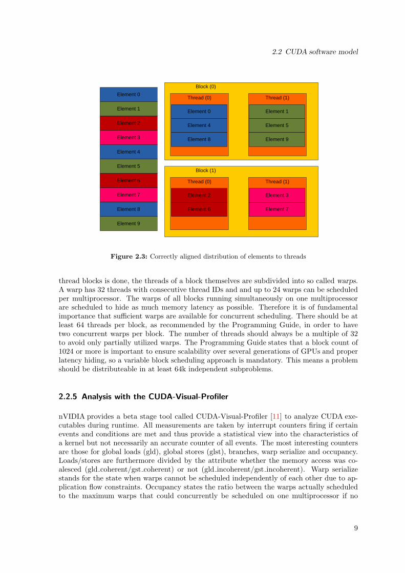
2.1 Model of the hardware of the nVIDIA G80 graphics processor . . . . . . . . . 42.2 Overview of the thread block batching of the CUDA software paradigm . . . 72.3 Correctly aligned distribution of elements to threads . . . . . . . . . . . . . . 9
3.1 Performance Streamcopy benchmark with vector length 220 and minimal blockand thread counts . . . . . . . . . . . . . . . . . . . . . . . . . . . . . . . . . 16
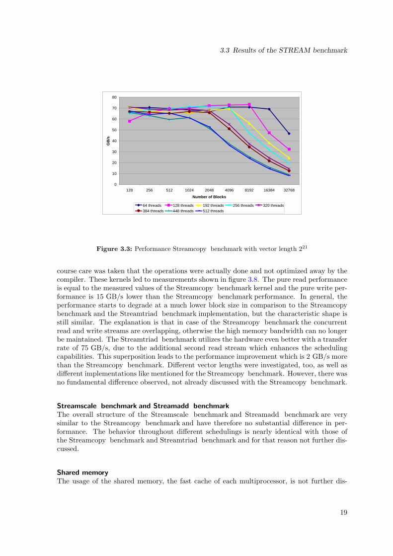
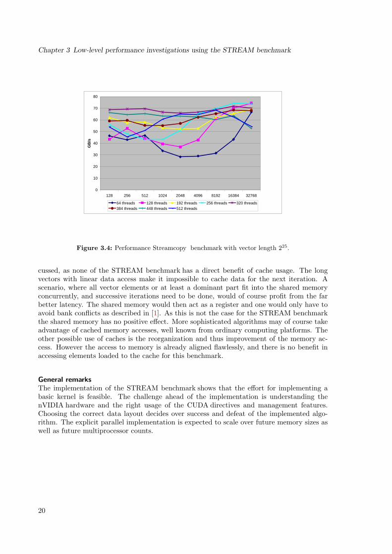
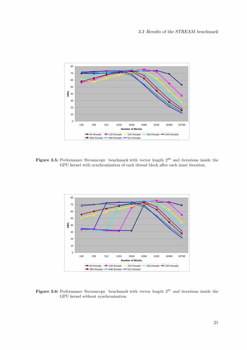
3.2 Performance Streamcopy benchmark with vector length 220 . . . . . . . . . . 173.3 Performance Streamcopy benchmark with vector length 221 . . . . . . . . . 183.4 Performance Streamcopy benchmark with vector length 225. . . . . . . . . . . 193.5 Performance Streamcopy benchmark with vector length 220 and iterations in-
side the GPU kernel with synchronization of each thread block after each inneriteration. . . . . . . . . . . . . . . . . . . . . . . . . . . . . . . . . . . . . . . 20
3.6 Performance Streamcopy benchmark with vector length 221 and iterations in-side the GPU kernel without synchronization. . . . . . . . . . . . . . . . . . . 20
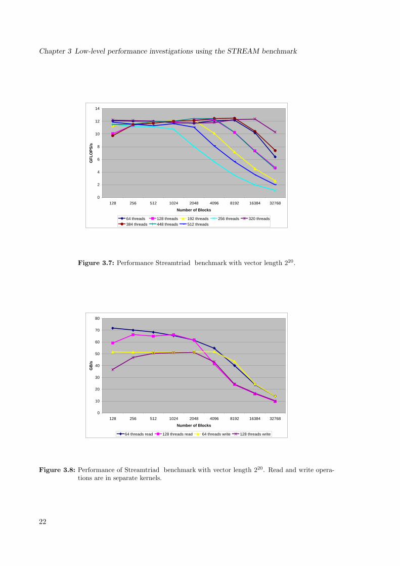
3.7 Performance Streamtriad benchmark with vector length 220. . . . . . . . . . 213.8 Performance of Streamtriad benchmark with vector length 220. Read and
write operations are in separate kernels. . . . . . . . . . . . . . . . . . . . . . 21
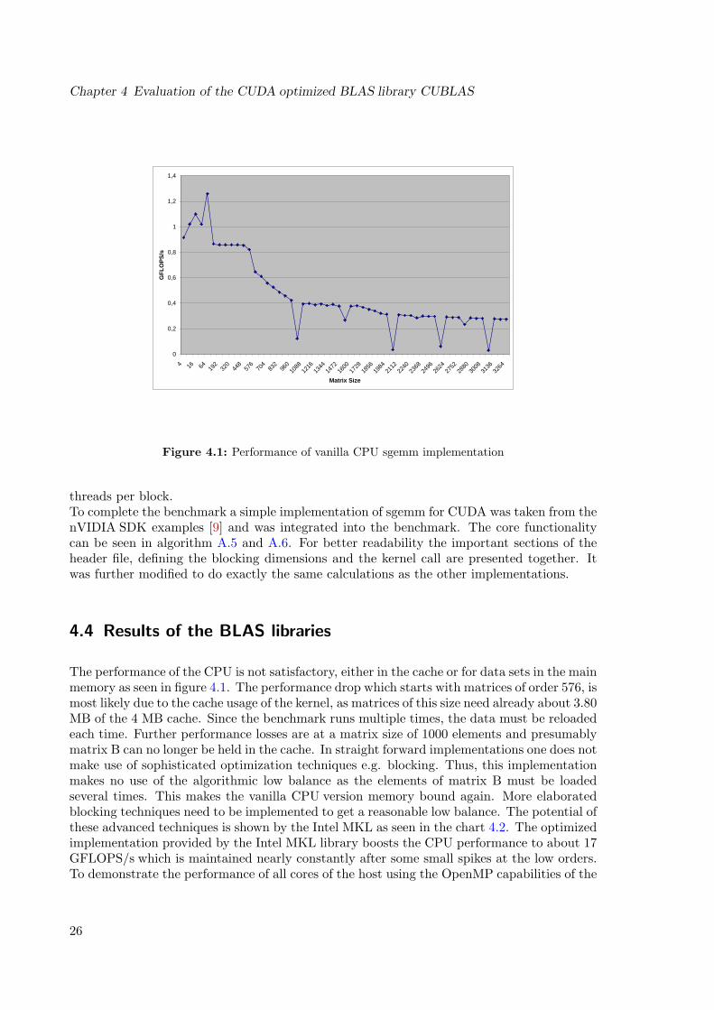
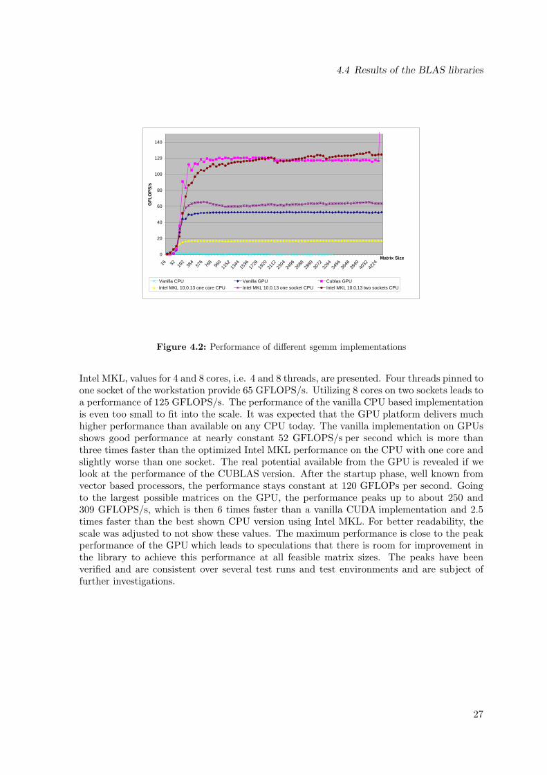
4.1 Performance of vanilla CPU sgemm implementation . . . . . . . . . . . . . . 254.2 Performance of different sgemm implementations . . . . . . . . . . . . . . . . 26
5.1 Discrete velocities in the D3Q19 model. . . . . . . . . . . . . . . . . . . . . . 295.2 Wrongly aligned distribution of elements to threads with array-of-structures . 335.3 Correctly aligned distribution of elements to threads with structure-of-arrays
layout . . . . . . . . . . . . . . . . . . . . . . . . . . . . . . . . . . . . . . . . 335.4 Mapping of lattice to blocks . . . . . . . . . . . . . . . . . . . . . . . . . . . . 345.5 Propagation to neighbor cells with different x-index . . . . . . . . . . . . . . . 375.6 Caching propagations in shared memory for aligned stores . . . . . . . . . . . 385.7 Aligned thread memory store of propagations . . . . . . . . . . . . . . . . . . 385.8 Performance for constant y- and z-dimension 32 and different x-domain sizes,
thus different number of scheduled threads. . . . . . . . . . . . . . . . . . . . 425.9 Performance for increased y- and z-dimension of 128 and different x-domain
sizes, thus different number of scheduled threads. . . . . . . . . . . . . . . . . 425.10 Performance for varying y and z-dimensions as function of the x-dimension
which is equal to the number of scheduled threads. . . . . . . . . . . . . . . . 435.11 Performance in FluidMLUPS/s over increasing cubic domain size for 1 and 8
threads using OpenMP parallelization on the CPU. . . . . . . . . . . . . . . . 435.12 Velocity profile in flow direction with periodic boundary condition applied in
y-direction . . . . . . . . . . . . . . . . . . . . . . . . . . . . . . . . . . . . . . 455.13 Pressure loss in direction of the flow for a 64x32x32 channel . . . . . . . . . . 46
iii
List of Figures
5.14 Pressure visualization along flow direction of a 64x32x32 channel . . . . . . . 465.15 Picture of the porous medium structure used as an example for flow in a
complex geometry. . . . . . . . . . . . . . . . . . . . . . . . . . . . . . . . . . 475.16 Pressure distribution in a cut along x-direction of the porous medium. . . . . 475.17 Velocity distribution in a cut along x-direction of the porous medium. . . . . 48
B.1 Performance Streamcopy with vector length 222 . . . . . . . . . . . . . . . . 68B.2 Performance Streamcopy with vector length 223 . . . . . . . . . . . . . . . . 69B.3 Performance Streamcopy with vector length 224 . . . . . . . . . . . . . . . . 69
iv
List of Tables
2.1 Host system specifications . . . . . . . . . . . . . . . . . . . . . . . . . . . . . 32.2 Graphics device specifications . . . . . . . . . . . . . . . . . . . . . . . . . . . 52.3 Register exclusively available for each thread on a nVIDIA G80 multiprocessor 5
3.1 Elements per block with 128 threads with vector length 220 . . . . . . . . . . 153.2 Elements per block with 128 threads with vector length 225 . . . . . . . . . . 153.3 Elements per block with 512 threads with vector length 225 . . . . . . . . . . 16
5.1 Concurrent blocks runnable due to register usage . . . . . . . . . . . . . . . . 39
C.1 Memory to operations balance of the STREAM benchmark . . . . . . . . . . 70C.2 Comparison of the memory to operations balance of the host system to the
G80 GPU. . . . . . . . . . . . . . . . . . . . . . . . . . . . . . . . . . . . . . 70
v

List of Tables
vi
List of Algorithms
2.1 Declaration and call of a CUDA Kernel (*.cu) . . . . . . . . . . . . . . . . . . 83.1 Golden CPU stream algorithm (*.c) . . . . . . . . . . . . . . . . . . . . . . . 143.2 Stream GPU kernel (*.cu) . . . . . . . . . . . . . . . . . . . . . . . . . . . . . 154.1 Allocation of memory on device (*.cu file) . . . . . . . . . . . . . . . . . . . . 234.2 Call of vanilla sgemm and Intel MKL library (*.c file) . . . . . . . . . . . . . 244.3 Call to CUBLAS library (*.c) . . . . . . . . . . . . . . . . . . . . . . . . . . . 275.1 Inner loop for consecutive iterations (*.cu) calling the GPU kernel . . . . . . 315.2 Outer loop for inside simulation output (*.cpp) calling the C wrapper routine 325.3 Access to particle distribution values via macro definition . . . . . . . . . . . 325.4 If statement, switching between bounce-back and propagation (*.cu) . . . . . 365.5 If statement, adjusting index for periodic boundary treatment (*.cu) . . . . . 405.6 Enhanced indexing for loading collision values from global memory (*.cu) . . 415.7 Enhanced indexing for propagation (*.cu) . . . . . . . . . . . . . . . . . . . . 41A.1 Memory allocation on device (*.cu) . . . . . . . . . . . . . . . . . . . . . . . . 52A.2 Memory initialization on device (*.cu) . . . . . . . . . . . . . . . . . . . . . . 52A.3 Vectorcopy CUDA kernel call (*.cu) . . . . . . . . . . . . . . . . . . . . . . . 52A.4 nVIDIA SDK disclaimer. . . . . . . . . . . . . . . . . . . . . . . . . . . . . . . 53A.5 Example from the nVIDIA SDK for matrix matrix multiplication (*.cu), header
and kernel call . . . . . . . . . . . . . . . . . . . . . . . . . . . . . . . . . . . 54A.6 Example from the nVIDIA SDK for matrix matrix multiplication (*.cu), kernel
implementation . . . . . . . . . . . . . . . . . . . . . . . . . . . . . . . . . . . 55A.7 Simplified code of the lattice Boltzmann flow solver implementation on the
GPU (*.cu) . . . . . . . . . . . . . . . . . . . . . . . . . . . . . . . . . . . . . 56
vii

Chapter 1
Introduction
General purpose central processing units (CPUs ) of the beginning 21st century try to keep upwith Moore’s law by continuously increasing the number of cores instead of further growingthe single core frequency. While on-chip thread parallelism is rather new for standard CPUs,graphics processing units (GPUs ) feature a massively parallel layout since long ago. In pastyears the use of GPUs was mainly restricted to the gaming industry for real time rendering.However, recently, this computing power has become more easily accessible for scientificand technical computing through more appropriate programming environments. Applicationprogramming interfaces (APIs) such as the “Compute Unified Device Architecture” (CUDA )from nVIDIA [9] and “Stream” from the AMD Graphics Products Group [3] became availablerecently and complement the graphics oriented interfaces like OpenGL [13] or Microsoft’sDirectX [6]. Nevertheless, GPUs have their own programming paradigms which must beunderstood in order to use them efficiently.
Looking closer at the typical operations, a graphics application operates huge amounts ofdata with mostly identical operations. In a similar manner scientific applications process datawith only little more diversity in operations. Hence, the link between both application areasis obvious; however, the programming approach of GPUs was not suited for non-graphicalapplications. The use of GPUs for numerical simulation has gained increased attention in thepast years. Lattice Boltzmann based flow solvers, e.g. Kaufmann et al. [26] and finite elementapplications, e.g. Goddeke et al. [19, 20] are only a few areas where first promising resultscould be obtained. A deep insight into the way graphics hardware works and its mapping tomathematical operations is required to implement the algorithms, and substantial time andeffort must be invested for successful porting. A first step by hardware vendors towards easingaccess to harnessing of this computational power has been taken by nVIDIA with the releaseof CUDA for the nVIDIA G80 GPU. The basic usage of CUDA is similar to OpenMP [12],as CUDA also extends the C language with several macros and functions. It is thereforetechnically possible to work with existing tools and environments to program the GPU.Although this approach to successfully and efficiently programming a GPU is still complexand uncommon, the CUDA framework is a first step towards a fully parallel programmingparadigm. First evaluations were done by Tolke et al. [31] for lattice Boltzmann methods andby Michalakes et al. [27] for numerical weather prediction, to name a few examples. Theseefforts show the potentials as well as the challenges arising with CUDA.
This thesis investigates programming techniques, parallelization approaches and optimizationstrategies and sheds some light on the potentials of using graphics processing units for numericand scientific applications.
1
Chapter 1 Introduction
This thesis is organized as follows. To understand the basic concepts and the fundamentaldifferences between CPUs and GPUs chapter 2 gives insight into the hardware specifications ofthe generic nVIDIA G80 core layout and the programming paradigms of the CUDA softwaretoolkit provided by nVIDIA. In chapter 3 the well known STREAM benchmark [15] is usedto classify the performance of the newly available architecture in relation to existing CPUplatforms. Libraries are used by many programmers to avoid complex adaptions of scientificcodes to new hardware developments. To address this, the usage and performance of thenVIDIA BLAS implementation called CUBLAS is evaluated in chapter 4. In chapter 5 theeffort and benefit of implementing a 3D lattice Boltzmann flow solver on GPUs is shown.Finally, chapter 6 summarizes the results and gives an outlook to future potentials anddevelopments in the field of GPU computing.
2
Chapter 2
Platform Overview
A detailed analysis of the hardware at hand is essential for any kind of platform, as one hasto know as much as possible about the underlying design. The information presented belowabout the Geforce 8800 GTX high-end graphics card, were mainly taken from the nVIDIAwebsite [7]. The description of the CUDA framework follows the guidelines given in theCUDA Programming Guide [1].
2.1 Hardware model
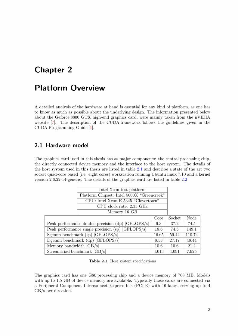
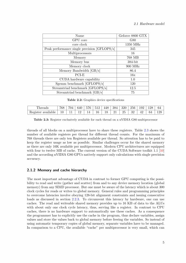
The graphics card used in this thesis has as major components: the central processing chip,the directly connected device memory and the interface to the host system. The details ofthe host system used in this thesis are listed in table 2.1 and describe a state of the art twosocket quad-core based (i.e. eight cores) workstation running Ubuntu linux 7.10 and a kernelversion 2.6.22-14-generic. The details of the graphics card are listed in table 2.2
Intel Xeon test platformPlatform Chipset: Intel 5000X “Greencreek”
CPU: Intel Xeon E 5345 “Clovertown”CPU clock rate: 2.33 GHz
Memory 16 GB
Core Socket NodePeak performance double precision (dp) [GFLOPS/s] 9.3 37.2 74.5Peak performance single precision (sp) [GFLOPS/s] 18.6 74.5 149.1Sgemm benchmark (sp) [GFLOPS/s] 16.65 59.44 110.74Dgemm benchmark (dp) [GFLOPS/s] 8.53 27.17 48.44Memory bandwidth [GB/s] 10.6 10.6 21.2Streamtriad benchmark [GB/s] 4.013 4.091 7.925
Table 2.1: Host system specifications
The graphics card has one G80 processing chip and a device memory of 768 MB. Modelswith up to 1.5 GB of device memory are available. Typically those cards are connected viaa Peripheral Component Interconnect Express bus (PCI-E) with 16 lanes, serving up to 4GB/s per direction.
3
Chapter 2 Platform Overview
Device
Device Memory
Multiprocessor N
Multiprocessor 2
Multiprocessor 1
TextureCache
ConstantCache
...Instruction
UnitRegisters Registers Registers
Processor 1 Processor 2 Processor M
Shared Memory
...
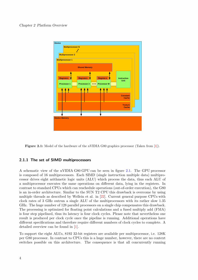
Figure 2.1: Model of the hardware of the nVIDIA G80 graphics processor (Taken from [1]).
2.1.1 The set of SIMD multiprocessors
A schematic view of the nVIDIA G80 GPU can be seen in figure 2.1. The GPU processoris composed of 16 multiprocessors. Each SIMD (single instruction multiple data) multipro-cessor drives eight arithmetic logic units (ALU) which process the data, thus each ALU ofa multiprocessor executes the same operations on different data, lying in the registers. Incontrast to standard CPUs which can reschedule operations (out-of-order execution), the G80is an in-order architecture. Similar to the SUN T2 CPU this drawback is overcome by usingmultiple threads as described by Wellein et al. in [22]. Current general purpose CPUs withclock rates of 3 GHz outrun a single ALU of the multiprocessors with its rather slow 1.35GHz. The huge number of 128 parallel processors on a single chip compensates this drawback.The processing is optimized for floating point calculations and a fused multiply add (FMA)is four step pipelined, thus its latency is four clock cycles. Please note that nevertheless oneresult is produced per clock cycle once the pipeline is running. Additional operations havedifferent specifications and therefore require different numbers of clock cycles to complete. Adetailed overview can be found in [1].
To support the eight ALUs, 8192 32-bit registers are available per multiprocessor, i.e. 128Kper G80 processor. In contrast to CPUs this is a huge number, however, there are no contextswitches possible on this architecture. The consequence is that all concurrently running
4
2.1 Hardware model
Name Geforce 8800 GTXGPU core G80core clock 1350 MHz
Peak performance single precision [GFLOPS/s] 345Multiprocessors 16
Memory 768 MBMemory bus 384-bit
Memory clock 900 MHzMemory Bandwidth [GB/s] 86.4
PCI-E 16xCUDA hardware capability 1.0
Sgemm benchmark [GFLOPS/s] 120Streamtriad benchmark [GFLOPS/s] 12.5
Streamtriad benchmark [GB/s] 75
Table 2.2: Graphics device specifications
Threads 768 704 640 576 512 448 384 320 256 192 128 64Register available 10 11 12 14 16 18 21 25 32 42 64 128
Table 2.3: Register exclusively available for each thread on a nVIDIA G80 multiprocessor
threads of all blocks on a multiprocessor have to share these registers. Table 2.3 shows thenumber of available registers per thread for different thread counts. For the maximum of768 threads there are only ten Registers available per thread. So attention has to be paid tokeep the register usage as low as possible. Similar challenges occur for the shared memoryas there are only 16K available per multiprocessor. Modern CPU architectures are equippedwith four to twelve MB of cache. The current version of the CUDA Software toolkit 1.1 [10]and the according nVIDIA G80 GPUs natively support only calculations with single precisionaccuracy.
2.1.2 Memory and cache hierarchy
The most important advantage of CUDA in contrast to former GPU computing is the possi-bility to read and write (gather and scatter) from and to any device memory location (globalmemory) from any SIMD processor. But one must be aware of the latency which is about 300clock cycles for reads or writes to global memory. General rules and programming principlesto overcome latencies involve obeying 128-bit alignment constraints and issuing consecutiveloads as discussed in section 2.2.3. To circumvent this latency by hardware, one can usecaches. The read and writeable shared memory provides up to 16 KB of data to the ALUswith about only one clock cycle latency, thus, serving like a register. In contrast to CPUcaches, there is no hardware support to automatically use these caches. As a consequencethe programmer has to explicitly use the cache in the program, thus declare variables, assignvalues and store the values back to global memory before freeing the variables. So instead ofusing automatic temporary copies of global memory, separate variables have to be managed.In comparison to a CPU, the available “cache” per multiprocessor is very small, which can
5
Chapter 2 Platform Overview
lead to problems owing to the execution scheduling further described in section 2.2.2. Theshared memory is organized in 16 32-bit banks. As long as all threads access different banksor only a single one, the shared memory has no penalty in comparison to register usageand no bank conflicts occur. Further on-chip memories, called constant or texture cache areavailable to the programmer, but were not applied in this thesis and are therefore not furtherdiscussed.
2.2 CUDA software model
The CUDA toolkit provides extensions to the C language and even integration into an C++environment is possible. This thesis only interfaces CUDA routines from plain C files. Someinput and output routines, running only on the host, are written in C++. In general, awrapper program is written in plain C and the calculation routines are out sourced to socalled GPU kernels. These GPU kernels have a certain calling syntax which specifies howthey are executed on the GPU. These parameters are recognized by the nVIDIA NVCCcompiler. The functionality below describes only the small subset used in this thesis.
2.2.1 Divide and conquer
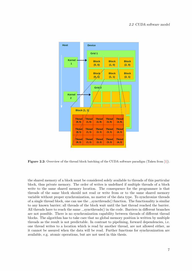
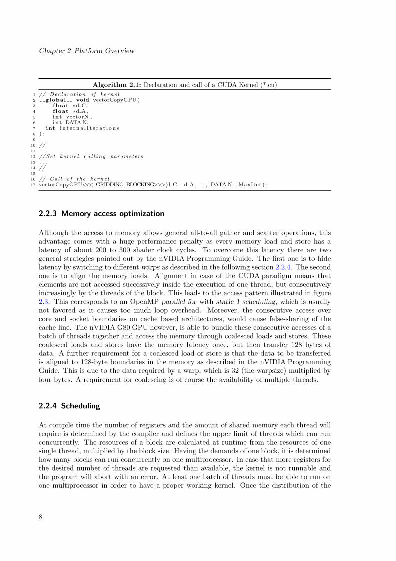
In order to run in parallel on 16 SIMD multiprocessors, the work has to be distributed amongthese processors. The host calls a GPU kernel. The amount of blocks and threads is specifiedvia the GPU kernel call. An example of a kernel declaration and call can be seen in algorithm2.1. All threads execute the GPU kernel. Threads are grouped together into blocks of threadsand are able to communicate over shared memory and can be synchronized. One block canhold up to 512 threads and must be executed on a single multiprocessor. Multiple blocks arebatched to a grid. Thus each GPU kernel is divided into a grid of thread blocks. Please notethat multiple blocks can run simultaneously on one single multiprocessor, however, the orderof execution is not defined. Blocks are addressable one or two dimensional, depending on thestructure of the program or on the preference of the programmer. Threads inside one block areaddressable using one, two and three dimensional thread indices. A graphical representationcan be seen in figure 2.2. To distribute work among blocks and threads, the programmercan use the ID of a thread (threadIdx.x, threadIdx.y, threadIdx.z), of a block (blockIdx.x,blockIdx.y) and the dimensions of the grid (gridDim.x, gridDim.y) and a block (blockDim.x,blockDim.y, blockDim.z). The amount of blocks and threads are passed to the GPU deviceby the kernel call. The first argument in the call of the kernel in algorithm 2.1 inside thespiky brackets defines the number of blocks, followed by the number of threads per block.Inside the standard brackets variables and arrays are passed to the kernel. The attribute
global defines a function which can only be called by the host and is then executed on thedevice.
2.2.2 Data coherence
With the GPU kernel call, the amount of shared memory per block is specified. As differentblocks may run on different multiprocessors (or with unspecified order on one multiprocessor),
6
2.2 CUDA software model
Host
Kernel 1
Kernel 2
Device
Grid 1
Block(0, 0)
Block(1, 0)
Block(2, 0)
Block(0, 1)
Block(1, 1)
Block(2, 1)
Grid 1
Block(0, 0)
Block(1, 0)
Block(2, 0)
Block(0, 0)
Block(1, 0)
Block(2, 0)
Block(0, 1)
Block(1, 1)
Block(2, 1)
Block(0, 1)
Block(1, 1)
Block(2, 1)
Grid 2Grid 2
Block (1, 1)
Thread(0, 1)
Thread(1, 1)
Thread(2, 1)
Thread(3, 1)
Thread(4, 1)
Thread(0, 2)
Thread(1, 2)
Thread(2, 2)
Thread(3, 2)
Thread(4, 2)
Thread(0, 0)
Thread(1, 0)
Thread(2, 0)
Thread(3, 0)
Thread(4, 0)
Block (1, 1)
Thread(0, 1)
Thread(1, 1)
Thread(2, 1)
Thread(3, 1)
Thread(4, 1)
Thread(0, 2)
Thread(1, 2)
Thread(2, 2)
Thread(3, 2)
Thread(4, 2)
Thread(0, 0)
Thread(1, 0)
Thread(2, 0)
Thread(3, 0)
Thread(4, 0)
Thread(0, 1)
Thread(1, 1)
Thread(2, 1)
Thread(3, 1)
Thread(4, 1)
Thread(0, 1)
Thread(1, 1)
Thread(2, 1)
Thread(3, 1)
Thread(4, 1)
Thread(0, 2)
Thread(1, 2)
Thread(2, 2)
Thread(3, 2)
Thread(4, 2)
Thread(0, 2)
Thread(1, 2)
Thread(2, 2)
Thread(3, 2)
Thread(4, 2)
Thread(0, 0)
Thread(1, 0)
Thread(2, 0)
Thread(3, 0)
Thread(4, 0)
Thread(0, 0)
Thread(1, 0)
Thread(2, 0)
Thread(3, 0)
Thread(4, 0)
Figure 2.2: Overview of the thread block batching of the CUDA software paradigm (Taken from [1]).
the shared memory of a block must be considered solely available to threads of this particularblock, thus private memory. The order of writes is undefined if multiple threads of a blockwrite to the same shared memory location. The consequence for the programmer is thatthreads of the same block should not read or write from or to the same shared memoryvariable without proper synchronization, no matter of the data type. To synchronize threadsof a single thread block, one can use the syncthreads() function. The functionality is similarto any known barrier; all threads of the block wait until the last thread reached the barrier.All threads have to reach the same syncthreads() in the code. Barriers in different branchesare not possible. There is no synchronization capability between threads of different threadblocks. The algorithm has to take care that no global memory position is written by multiplethreads as the result is not predictable. In contrast to pipelining, forward dependencies, i.e.one thread writes to a location which is read by another thread, are not allowed either, asit cannot be assured when the data will be read. Further functions for synchronization areavailable, e.g. atomic operations, but are not used in this thesis.
7
Chapter 2 Platform Overview
Algorithm 2.1: Declaration and call of a CUDA Kernel (*.cu)1 // Dec lara t ion o f k e rne l2 global void vectorCopyGPU (3 f loat ∗d C ,4 f loat ∗d A ,5 int vectorN ,6 int DATA N,7 int i n t e r n a l I t e r a t i o n s8 ) ;9
10 //11 . . .12 // Set ke rne l c a l l i n g parameters13 . . .14 //15
16 // Ca l l o f the ke rne l17 vectorCopyGPU<<< GRIDDING,BLOCKING>>>(d C , d A , 1 , DATA N, MaxIter ) ;
2.2.3 Memory access optimization
Although the access to memory allows general all-to-all gather and scatter operations, thisadvantage comes with a huge performance penalty as every memory load and store has alatency of about 200 to 300 shader clock cycles. To overcome this latency there are twogeneral strategies pointed out by the nVIDIA Programming Guide. The first one is to hidelatency by switching to different warps as described in the following section 2.2.4. The secondone is to align the memory loads. Alignment in case of the CUDA paradigm means thatelements are not accessed successively inside the execution of one thread, but consecutivelyincreasingly by the threads of the block. This leads to the access pattern illustrated in figure2.3. This corresponds to an OpenMP parallel for with static 1 scheduling, which is usuallynot favored as it causes too much loop overhead. Moreover, the consecutive access overcore and socket boundaries on cache based architectures, would cause false-sharing of thecache line. The nVIDIA G80 GPU however, is able to bundle these consecutive accesses of abatch of threads together and access the memory through coalesced loads and stores. Thesecoalesced loads and stores have the memory latency once, but then transfer 128 bytes ofdata. A further requirement for a coalesced load or store is that the data to be transferredis aligned to 128-byte boundaries in the memory as described in the nVIDIA ProgrammingGuide. This is due to the data required by a warp, which is 32 (the warpsize) multiplied byfour bytes. A requirement for coalescing is of course the availability of multiple threads.
2.2.4 Scheduling
At compile time the number of registers and the amount of shared memory each thread willrequire is determined by the compiler and defines the upper limit of threads which can runconcurrently. The resources of a block are calculated at runtime from the resources of onesingle thread, multiplied by the block size. Having the demands of one block, it is determinedhow many blocks can run concurrently on one multiprocessor. In case that more registers forthe desired number of threads are requested than available, the kernel is not runnable andthe program will abort with an error. At least one batch of threads must be able to run onone multiprocessor in order to have a proper working kernel. Once the distribution of the
8
2.2 CUDA software model
Element 0
Element 1
Element 5
Element 4
Element 3
Element 2
Element 6
Element 7
Element 9
Element 8
Block (0)
Thread (1)
Element 1
Element 5
Element 9
Thread (0)
Element 0
Element 4
Element 8
Block (1)
Thread (1)
Element 3
Element 7
Thread (0)
Element 2
Element 6
Figure 2.3: Correctly aligned distribution of elements to threads
thread blocks is done, the threads of a block themselves are subdivided into so called warps.A warp has 32 threads with consecutive thread IDs and and up to 24 warps can be scheduledper multiprocessor. The warps of all blocks running simultaneously on one multiprocessorare scheduled to hide as much memory latency as possible. Therefore it is of fundamentalimportance that sufficient warps are available for concurrent scheduling. There should be atleast 64 threads per block, as recommended by the Programming Guide, in order to havetwo concurrent warps per block. The number of threads should always be a multiple of 32to avoid only partially utilized warps. The Programming Guide states that a block count of1024 or more is important to ensure scalability over several generations of GPUs and properlatency hiding, so a variable block scheduling approach is mandatory. This means a problemshould be distributeable in at least 64k independent subproblems.
2.2.5 Analysis with the CUDA-Visual-Profiler
nVIDIA provides a beta stage tool called CUDA-Visual-Profiler [11] to analyze CUDA exe-cutables during runtime. All measurements are taken by interrupt counters firing if certainevents and conditions are met and thus provide a statistical view into the characteristics ofa kernel but not necessarily an accurate counter of all events. The most interesting countersare those for global loads (gld), global stores (glst), branches, warp serialize and occupancy.Loads/stores are furthermore divided by the attribute whether the memory access was co-alesced (gld coherent/gst coherent) or not (gld incoherent/gst incoherent). Warp serializestands for the state when warps cannot be scheduled independently of each other due to ap-plication flow constraints. Occupancy states the ratio between the warps actually scheduledto the maximum warps that could concurrently be scheduled on one multiprocessor if no
9
Chapter 2 Platform Overview
register or shared memory usage constraints would exist. The tool is used to quickly probea new implementation and find major performance problems.
2.2.6 The CUDA compiler driver NVCC
The compiler provided by nVIDIA to compile GPU kernel (*.cu) files is called NVCC [8]. Allimplementations where compiled with the NVCC option -O3 for maximum optimizations.Interesting for performance analysis is the intermediate *.cubin file produced by specifying-cubin as a compiler flag. The file contains for every kernel the number of registers as well asthe shared and the local memory occupied during runtime on the GPU. In case of the sharedmemory one has to add the amount of shared memory which is dynamically allocated onceper block. The compiler option –maxrregcount limits the registers the compiled kernel mayuse during runtime. Please note that this might come with the cost of additional loads andstores to memory. To get a deep insight into the compiled program structure the assemblyoutput can be viewed by adding the options -keep -opencc-options -LIST:source=on –ptxas-options=-v to the NVCC compiler flags.
2.3 Metrices
Performance MetricesTwo different performance metrices are applied in this thesis. For three out of four streamtests, one has the choice to use the widely used GFLOPS/s, standing for giga (109) floating-point-operations per second, as well as GB/s, standing for giga (109) bytes per second. Forchapter 5 the metric FluidMLUPS/s, meaning mega (106) lattice-site-updates per secondis used. This measures the number of cell updates per second, independently from theunderlying implementation and thus is comparable even throughout different implementationsand different architectures of the same model. Please note to compare between measurementsbenchmarked with the same level of accuracy (single precision).
BalanceThe balance is defined by equation 2.1
balance =memory transfers per cycle [words]floating operations per cycle [flop]
(2.1)
and is applicable to algorithms (cycle regards to one iteration step) and computing hardware.Be reminded that, in the present context, a word directly corresponds to a single precisionfloating point variable, i.e. 4 bytes. Therefore a balance smaller than 1.0 describes a systemwhich can load less than one single operand per flop. On the other hand a balance larger thanone defines a system which can deliver more words than execute floating point operations.Common balances for desktop PCs are about 0.05 (sustained), whereas vector hardware hasbalances of up to 0.5. Even a simple operation like the scalar product has a balance of oneword per flop and usually more than one operand is necessary per flop. Please note that thereare algorithms, e.g. the lattice Boltzmann method described in chapter 5, that have a balancesmaller one. Best usage of the underlying hardware can only be achieved if the balance of the
10
2.3 Metrices
hardware is higher than the balance of the algorithm. Nevertheless these are rare cases andtherefore algorithms have to be improved to exploit the hardware characteristics. The evergrowing DRAM-gap, i.e. the increasing discrepancy of arithmetic and memory operations,leads to lower balances with each platform generation. Still, the overall performance of theplatform might improve.
11

Chapter 2 Platform Overview
12
Chapter 3
Low-level performance investigations usingthe STREAM benchmark
As chapter 2 shows, the architecture of todays GPUs is very sophisticated. For data inten-sive applications, e.g. lattice Boltzmann methods, the attainable memory bandwidth is thelimiting factor. Memory hardware shows a large gap between theoretical peak performanceand sustainable performance. The STREAM benchmark is used to evaluate and substantiallydifferentiate the GPU based platform from CPUs. This is usually the first step, before opti-mizing more sophisticated algorithms as it provides knowledge about attainable performanceand about the hardware.
3.1 The STREAM benchmark
The STREAM benchmark [15] is a collection of vector based algorithms. These algorithmsput stress on the memory transfer capability of a hardware platform. The STREAM bench-mark consists of the copy, scale, add and the triad. The simple kernels of the STREAMbenchmark can be seen in algorithm 3.1 for the CPU and in algorithm 3.2 for the GPU,where #ifdef macros define which kernel to execute. Having a vector with N elements meansfor the Streamcopy benchmark and Streamscale benchmark a memory transfer of overallN · 2 · 4 bytes. Accordingly for the Streamadd benchmark and Streamtriad benchmark wefind overall N · 3 · 4 bytes to transfer. The Streamscale benchmark and Streamadd bench-mark count N operations and the Streamtriad benchmark has N ·2 operations. The differentbalances are 2.0 for the Streamscale benchmark, 3.0 for the Streamadd benchmark and 1.5for the Streamtriad benchmark as shown in table C.1.
Based on the hardware characteristics from table 2.1 and 2.2 the balance of the host system,using the theoretical memory bandwidth, is 0.034 and the GPU balance is 0.25 as shown intable C.2. Even though the GPU balance is much better than the balance of the host systemit is still not likely that the arithmetic performance could limit the benchmark results. Incontrast to common CPUs and their cache hierarchy a ”read-for-ownership” (RFO) prior towriting data is not necessary. So for each write to global memory only one transfer takes place,i.e. four bytes in contrast to eight bytes on CPUs. So the sustainable memory bandwidth ofthe CPU and thus the balance is less than the calculated values and is furthermore decreasedby an inefficient memory interface, whereas the GPU values hold.
13
Chapter 3 Low-level performance investigations using the STREAM benchmark
3.2 Implementation of the STREAM benchmark
The implementation of the STREAM benchmark was divided in three major parts. Firsta simple vanilla kernel or golden kernel was implemented which performed the particularalgorithm on the CPU. This served to check the GPUs results for correctness. The codeof the Streamcopy benchmark algorithm is shown in algorithm 3.1. The CUDA memoryallocation and the initialization can be seen in algorithm A.1 and A.2. The GPU kernel callin algorithm A.3 and the GPU kernel itself shown in algorithm 3.2 completes the Streamcopybenchmark. Of course for verifying proper calculations, the data is copied back from thedevice and cross checked to the golden CPU kernel results. Arrays residing on the host willalways be prefixed by a h , arrays placed on the device with d . This is only due to betterreadability. For measuring the impact of the kernel call overhead a kernel which was calledfor each iteration and a kernel which performed the iteration loop on its own were tested.
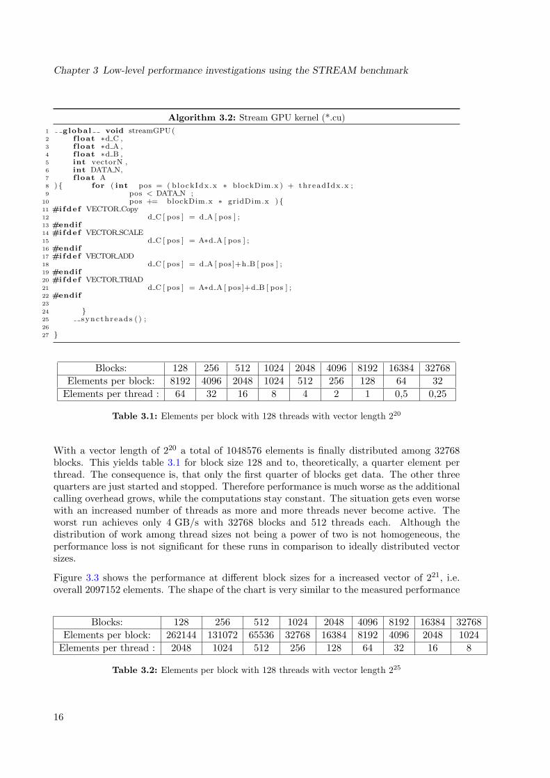
Workload data distribution with the CUDA programming paradigmThe main task of implementing a computational kernel for a GPU is the distribution of thework among the threads. The for loop from line 8 to 24 in algorithm 3.2 distributes thecomputational domain, based on an one dimensional grid layout and an one dimensionalblock layout. As pointed out by the nVIDIA CUDA Programming Guide [1] and shown insection 2.2.3, one should use a base address and then distribute the kernel operations amongall threads. In contrast to well known scheduling strategies, e.g. OpenMP, the whole domainis not decomposed based on its overall dimensions but element by element. This yields theadvantage that the remaining odd elements are treated automatically and no additional carehas to be taken, no matter how good the dimensions of the computational domain fit intothe grid and block dimensions. This distribution is illustrated in figure 2.3. Of course, thereare some drawbacks in performance compared to equally distributed work among threadsthat can be adjusted by the vector length. For vectors, whose length is a power of two thedistribution always is very homogeneous, at least if the amount of threads meets this criteriatoo. The for loop starts at the base address for every thread, which is calculated from theblock index blockIdx.x and the block dimension blockDim.x, both in x direction. Of coursethe positioning counter has to stay between the first and last element of the domain, whichis ensured with the second for-loop argument. For the increment, one has to consider thatevery thread within all blocks runs synchronously. As a consequence, the increment must beexactly the number of threads in one grid. This is achieved by blockDim.x · gridDim.x. Formore sophisticated thread and block decomposition strategies, two or three dimensional, onehas to adjust the base address and increment accordingly.
3.3 Results of the STREAM benchmark
The performance charts presented in this chapter show the sustained performance in GB/sor GFLOPS/s for increasing amounts of blocks while the problem size remains constant. Thedifferent graphs represent the number of threads each block has. As mentioned in table 2.2the maximum achievable memory bandwidth is about 86.4 GB/s for this particular GPU.The upcoming question is, what scheduling parameter or set of parameters should be used
14

3.3 Results of the STREAM benchmark
Algorithm 3.1: Golden CPU stream algorithm (*.c)1 extern ”C”2 void streamCPU(3 f loat ∗h C ,4 f loat ∗h A ,5 f loat ∗h B ,6 int vectorN ,7 int DATA N,8 f loat A9 ) {
10 for ( int pos =0; pos < DATA N ; pos ++){11
12 #ifdef VECTOR COPY13 h C [ pos ] = h A [ pos ] ;14 #endif15
16 #ifdef VECTOR SCALE17 h C [ pos ] = A∗h A [ pos ] ;18 #endif19
20 #ifdef VECTOR ADD21 h C [ pos ] = h A [ pos ]+h B [ pos ] ;22 #endif23
24 #ifdef VECTOR TRIAD25 h C [ pos ] = A∗h A [ pos ]+h B [ pos ] ;26 #endif27
28 }29 }
in order to exploit the hardware as much as possible and to get feasible results.
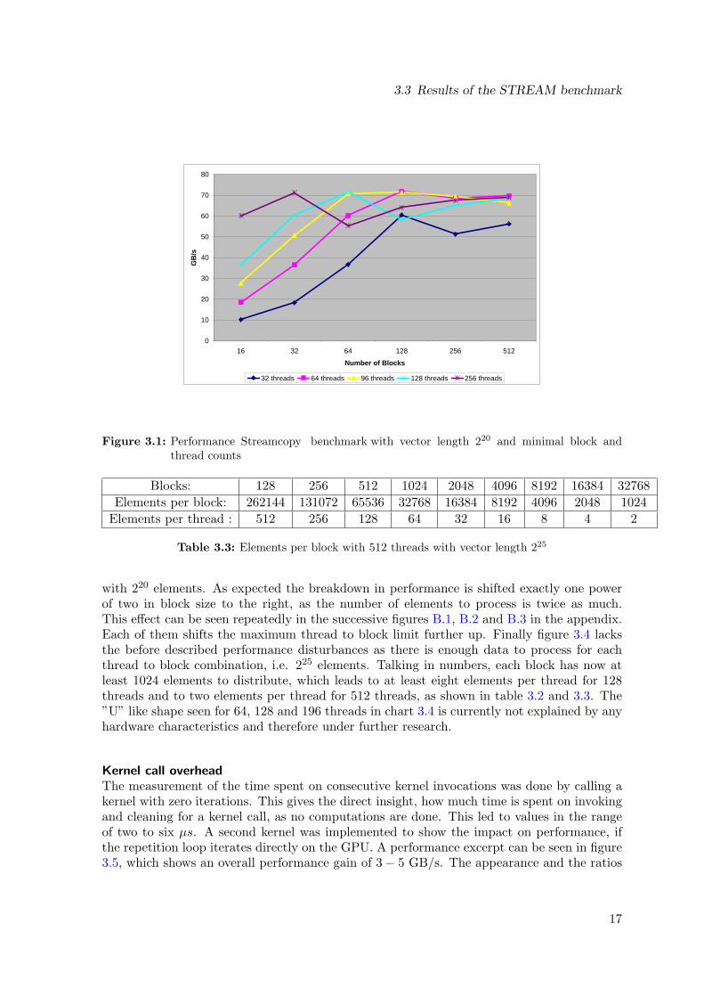
As one can see in chart 3.1 the performance of the Streamcopy benchmark starts with low10 GB/s for 16 blocks and 32 threads per block, i.e. 512 threads in total. This is due to thehard- and software constraints mentioned in detail in chapter 2. As one block can only runon one multiprocessor, 16 blocks provide no possibility for the hardware to schedule differentblocks on one multiprocessor concurrently without empty multiprocessors. Furthermore 32threads as a warp are the smallest package one multiprocessor can schedule. So the memorybandwidth cannot be enhanced by proper latency hiding. With a growing amount of blocksthe situation improves but is restricted by a maximum number of 8 blocks per multiprocessor.With higher thread counts the situation is better and improves to a level of about 70 GB/s.The general shape of the performance graph is very similar to vector processors wind upphase, however the problem size is not changed but the distribution. With at least 256threads per block there is no startup behavior anymore. The following charts in this chapterwill only present performance values at meaningful thread and block counts, starting at 64threads to enable two independent warps per block and 128 blocks to have 8 blocks permultiprocessor from the start, i.e. 8192 threads in total.
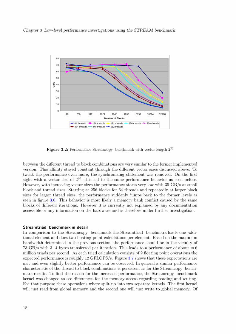
The measurements of the Streamcopy benchmark in chart 3.2 show the performance peak of74 GB/s with 4096 blocks and 128 threads, i.e. 84% of the achievable memory performance.These measurements were done with the current available CUDA version 1.1. Measurementswith the former Version 1.0 showed slightly worse results. A sustained performance of at least65 GB/s is maintained by nearly every variety of block to thread combination in the left partof the chart. The decreasing performance, starting at 1024 to 2048 blocks following down thex-axis becomes obvious if one determines the work distribution to one block or per thread.
15
Chapter 3 Low-level performance investigations using the STREAM benchmark
Algorithm 3.2: Stream GPU kernel (*.cu)1 global void streamGPU(2 f loat ∗d C ,3 f loat ∗d A ,4 f loat ∗d B ,5 int vectorN ,6 int DATA N,7 f loat A8 ) { for ( int pos = ( b lock Idx .x ∗ blockDim.x ) + threadIdx .x ;9 pos < DATA N ;
10 pos += blockDim.x ∗ gridDim.x ) {11 #ifdef VECTOR Copy12 d C [ pos ] = d A [ pos ] ;13 #endif14 #ifdef VECTOR SCALE15 d C [ pos ] = A∗d A [ pos ] ;16 #endif17 #ifdef VECTOR ADD18 d C [ pos ] = d A [ pos ]+h B [ pos ] ;19 #endif20 #ifdef VECTOR TRIAD21 d C [ pos ] = A∗d A [ pos ]+d B [ pos ] ;22 #endif23
24 }25 sync th r ead s ( ) ;26
27 }
Blocks: 128 256 512 1024 2048 4096 8192 16384 32768Elements per block: 8192 4096 2048 1024 512 256 128 64 32
Elements per thread : 64 32 16 8 4 2 1 0,5 0,25
Table 3.1: Elements per block with 128 threads with vector length 220
With a vector length of 220 a total of 1048576 elements is finally distributed among 32768blocks. This yields table 3.1 for block size 128 and to, theoretically, a quarter element perthread. The consequence is, that only the first quarter of blocks get data. The other threequarters are just started and stopped. Therefore performance is much worse as the additionalcalling overhead grows, while the computations stay constant. The situation gets even worsewith an increased number of threads as more and more threads never become active. Theworst run achieves only 4 GB/s with 32768 blocks and 512 threads each. Although thedistribution of work among thread sizes not being a power of two is not homogeneous, theperformance loss is not significant for these runs in comparison to ideally distributed vectorsizes.
Figure 3.3 shows the performance at different block sizes for a increased vector of 221, i.e.overall 2097152 elements. The shape of the chart is very similar to the measured performance
Blocks: 128 256 512 1024 2048 4096 8192 16384 32768Elements per block: 262144 131072 65536 32768 16384 8192 4096 2048 1024
Elements per thread : 2048 1024 512 256 128 64 32 16 8
Table 3.2: Elements per block with 128 threads with vector length 225
16
3.3 Results of the STREAM benchmark
0
10
20
30
40
50
60
70
80
16 32 64 128 256 512
Number of Blocks
GB
/s
32 threads 64 threads 96 threads 128 threads 256 threads
Figure 3.1: Performance Streamcopy benchmark with vector length 220 and minimal block andthread counts
Blocks: 128 256 512 1024 2048 4096 8192 16384 32768Elements per block: 262144 131072 65536 32768 16384 8192 4096 2048 1024
Elements per thread : 512 256 128 64 32 16 8 4 2
Table 3.3: Elements per block with 512 threads with vector length 225
with 220 elements. As expected the breakdown in performance is shifted exactly one powerof two in block size to the right, as the number of elements to process is twice as much.This effect can be seen repeatedly in the successive figures B.1, B.2 and B.3 in the appendix.Each of them shifts the maximum thread to block limit further up. Finally figure 3.4 lacksthe before described performance disturbances as there is enough data to process for eachthread to block combination, i.e. 225 elements. Talking in numbers, each block has now atleast 1024 elements to distribute, which leads to at least eight elements per thread for 128threads and to two elements per thread for 512 threads, as shown in table 3.2 and 3.3. The”U” like shape seen for 64, 128 and 196 threads in chart 3.4 is currently not explained by anyhardware characteristics and therefore under further research.
Kernel call overheadThe measurement of the time spent on consecutive kernel invocations was done by calling akernel with zero iterations. This gives the direct insight, how much time is spent on invokingand cleaning for a kernel call, as no computations are done. This led to values in the rangeof two to six µs. A second kernel was implemented to show the impact on performance, ifthe repetition loop iterates directly on the GPU. A performance excerpt can be seen in figure3.5, which shows an overall performance gain of 3− 5 GB/s. The appearance and the ratios
17
Chapter 3 Low-level performance investigations using the STREAM benchmark
0
10
20
30
40
50
60
70
80
128 256 512 1024 2048 4096 8192 16384 32768
Number of Blocks
GB
/s
64 threads 128 threads 192 threads 256 threads 320 threads384 threads 448 threads 512 threads
Figure 3.2: Performance Streamcopy benchmark with vector length 220
between the different thread to block combinations are very similar to the former implementedversion. This affinity stayed constant through the different vector sizes discussed above. Totweak the performance even more, the synchronizing statement was removed. On the firstsight with a vector size of 220, this led to the same performance behavior as seen before.However, with increasing vector sizes the performance starts very low with 35 GB/s at smallblock and thread sizes. Starting at 256 blocks for 64 threads and repeatedly at larger blocksizes for larger thread sizes, the performance suddenly jumps back to the former levels asseen in figure 3.6. This behavior is most likely a memory bank conflict caused by the sameblocks of different iterations. However it is currently not explained by any documentationaccessible or any information on the hardware and is therefore under further investigation.
Streamtriad benchmark in detailIn comparison to the Streamcopy benchmark the Streamtriad benchmark loads one addi-tional element and does two floating point calculations per element. Based on the maximumbandwidth determined in the previous section, the performance should be in the vicinity of73 GB/s with 3 · 4 bytes transferred per iteration. This leads to a performance of about ≈ 6million triads per second. As each triad calculation consists of 2 floating point operations theexpected performance is roughly 12 GFLOPS/s. Figure 3.7 shows that these expectations aremet and even slightly better performance can be observed. In general a similar performancecharacteristic of the thread to block combinations is persistent as for the Streamcopy bench-mark results. To find the reason for the increased performance, the Streamcopy benchmarkkernel was changed to see differences for the memory access regarding reading and writing.For that purpose these operations where split up into two separate kernels. The first kernelwill just read from global memory and the second one will just write to global memory. Of
18
3.3 Results of the STREAM benchmark
0
10
20
30
40
50
60
70
80
128 256 512 1024 2048 4096 8192 16384 32768
Number of Blocks
GB
/s
64 threads 128 threads 192 threads 256 threads 320 threads384 threads 448 threads 512 threads
Figure 3.3: Performance Streamcopy benchmark with vector length 221
course care was taken that the operations were actually done and not optimized away by thecompiler. These kernels led to measurements shown in figure 3.8. The pure read performanceis equal to the measured values of the Streamcopy benchmark kernel and the pure write per-formance is 15 GB/s lower than the Streamcopy benchmark performance. In general, theperformance starts to degrade at a much lower block size in comparison to the Streamcopybenchmark and the Streamtriad benchmark implementation, but the characteristic shape isstill similar. The explanation is that in case of the Streamcopy benchmark the concurrentread and write streams are overlapping, otherwise the high memory bandwidth can no longerbe maintained. The Streamtriad benchmark utilizes the hardware even better with a transferrate of 75 GB/s, due to the additional second read stream which enhances the schedulingcapabilities. This superposition leads to the performance improvement which is 2 GB/s morethan the Streamcopy benchmark. Different vector lengths were investigated, too, as well asdifferent implementations like mentioned for the Streamcopy benchmark. However, there wasno fundamental difference observed, not already discussed with the Streamcopy benchmark.
Streamscale benchmark and Streamadd benchmarkThe overall structure of the Streamscale benchmark and Streamadd benchmark are verysimilar to the Streamcopy benchmark and have therefore no substantial difference in per-formance. The behavior throughout different schedulings is nearly identical with those ofthe Streamcopy benchmark and Streamtriad benchmark and for that reason not further dis-cussed.
Shared memoryThe usage of the shared memory, the fast cache of each multiprocessor, is not further dis-
19
Chapter 3 Low-level performance investigations using the STREAM benchmark
0
10
20
30
40
50
60
70
80
128 256 512 1024 2048 4096 8192 16384 32768
Number of Blocks
GB
/s
64 threads 128 threads 192 threads 256 threads 320 threads384 threads 448 threads 512 threads
Figure 3.4: Performance Streamcopy benchmark with vector length 225.
cussed, as none of the STREAM benchmark has a direct benefit of cache usage. The longvectors with linear data access make it impossible to cache data for the next iteration. Ascenario, where all vector elements or at least a dominant part fit into the shared memoryconcurrently, and successive iterations need to be done, would of course profit from the farbetter latency. The shared memory would then act as a register and one would only have toavoid bank conflicts as described in [1]. As this is not the case for the STREAM benchmarkthe shared memory has no positive effect. More sophisticated algorithms may of course takeadvantage of cached memory accesses, well known from ordinary computing platforms. Theother possible use of caches is the reorganization and thus improvement of the memory ac-cess. However the access to memory is already aligned flawlessly, and there is no benefit inaccessing elements loaded to the cache for this benchmark.
General remarksThe implementation of the STREAM benchmark shows that the effort for implementing abasic kernel is feasible. The challenge ahead of the implementation is understanding thenVIDIA hardware and the right usage of the CUDA directives and management features.Choosing the correct data layout decides over success and defeat of the implemented algo-rithm. The explicit parallel implementation is expected to scale over future memory sizes aswell as future multiprocessor counts.
20
3.3 Results of the STREAM benchmark
0
10
20
30
40
50
60
70
80
128 256 512 1024 2048 4096 8192 16384 32768
Number of Blocks
GB
/s
64 threads 128 threads 192 threads 256 threads 320 threads384 threads 448 threads 512 threads
Figure 3.5: Performance Streamcopy benchmark with vector length 220 and iterations inside theGPU kernel with synchronization of each thread block after each inner iteration.
0
10
20
30
40
50
60
70
80
128 256 512 1024 2048 4096 8192 16384 32768
Number of Blocks
GB
/s
64 threads 128 threads 192 threads 256 threads 320 threads384 threads 448 threads 512 threads
Figure 3.6: Performance Streamcopy benchmark with vector length 221 and iterations inside theGPU kernel without synchronization.
21
Chapter 3 Low-level performance investigations using the STREAM benchmark
0
2
4
6
8
10
12
14
128 256 512 1024 2048 4096 8192 16384 32768
Number of Blocks
GFL
OPS
/s
64 threads 128 threads 192 threads 256 threads 320 threads384 threads 448 threads 512 threads
Figure 3.7: Performance Streamtriad benchmark with vector length 220.
0
10
20
30
40
50
60
70
80
128 256 512 1024 2048 4096 8192 16384 32768
Number of Blocks
GB
/s
64 threads read 128 threads read 64 threads write 128 threads write
Figure 3.8: Performance of Streamtriad benchmark with vector length 220. Read and write opera-tions are in separate kernels.
22
Chapter 4
Evaluation of the CUDA optimized BLASlibrary CUBLAS
Chapter 3 showed the basic potential of the nVIDIA G80 architecture. However, not everyoneis willing to put that much effort into programming a single kernel which is then highlyoptimized, but limited to this particular platform. In contrast, a lot of scientific applicationstake advantage of a huge variety of optimized libraries. The libraries itself are maintainedand optimized for several platforms. Very popular are the BLAS (Basic Linear AlgebraicSubroutines) which are included in e.g. Intel MKL [5], AMD ACML [2] or the publiclyavailable ATLAS library [4]. Through a common BLAS interface, the optimal library islinked into the program. Only the degree and focus of optimization is different. Instead ofadjusting a program to a particular platform, one chooses the optimal library and outsourcesall time consuming routines to libraries, if possible. This way a program can exist over severalgenerations of computer designs and still maintain satisfactory performance. The aim of thischapter is to check how easy the integration of nVIDIA’s BLAS library is and how muchperformance can be gained.
4.1 The level 3 BLAS routine sgemm
The BLAS libraries are subdivided in 3 levels, where level 1 involves only vectors, level 2vectors and matrices and level 3 only matrices. As chapter 3 already dealt with custom CUDAimplementations of some level 1 routines, we focused now on a specific level 3 routine, namelysgemm. Sgemm does a Single precision GEneral Matrix Matrix multiply. A simple CPUimplementation (vanilla CPU) of this can be seen in algorithm 4.2, function simple sgemm(lines 1 to 17). By means of complexity the multiplication of N2 matrix elements needsO(N3) floating point operations performed on O(N2) data items. So in contrast to the level1 and 2 routines, this kernel may have a low memory to floating-point-operation balance.
4.2 Preparations for the libraries
The necessary memory for the matrices on the host is allocated as seen in algorithm 4.1 (lines1 to 9). For better readability any error checking was removed from the algorithm. Arraysresiding on the host will always be prefixed by a h , arrays placed on the device with d . This
23
Chapter 4 Evaluation of the CUDA optimized BLAS library CUBLAS
Algorithm 4.1: Allocation of memory on device (*.cu file)1 /∗ Al l o ca t e hos t memory fo r the matr ices ∗/2 h A = ( f loat ∗) mal loc ( n2 ∗ s izeof ( h A [ 0 ] ) ) ;3
4 h B = ( f loat ∗) mal loc ( n2 ∗ s izeof ( h B [ 0 ] ) ) ;5
6 h C = ( f loat ∗) mal loc ( n2 ∗ s izeof ( h C [ 0 ] ) ) ;7
8
9 h C re f = ( f loat ∗) mal loc ( n2 ∗ s izeof ( h C [ 0 ] ) ) ;10
11
12 /∗ F i l l the matr ices with t e s t data ∗/13 for ( i = 0 ; i < n2 ; i++) {14 h A [ i ] = rand ( ) / ( f loat )RAND MAX;15 h B [ i ] = rand ( ) / ( f loat )RAND MAX;16 h C [ i ] = rand ( ) / ( f loat )RAND MAX;17 }18
19
20 /∗ Al l o ca t e dev i ce memory fo r the matr ices ∗/21 s t a t u s = cub la sA l l o c ( n2 , s izeof ( d A [ 0 ] ) , (void ∗∗)&d A ) ;22
23 s t a t u s = cub la sA l l o c ( n2 , s izeof ( d B [ 0 ] ) , (void ∗∗)&d B ) ;24
25 s t a t u s = cub la sA l l o c ( n2 , s izeof ( d C [ 0 ] ) , (void ∗∗)&d C ) ;26
27
28 /∗ I n i t i a l i z e the dev i ce matr ices with the hos t matr ices ∗/29 s t a t u s = cublasSetVector ( n2 , s izeof ( h A [ 0 ] ) , h A , 1 , d A , 1) ;30
31 s t a t u s = cublasSetVector ( n2 , s izeof ( h B [ 0 ] ) , h B , 1 , d B , 1) ;32
33 s t a t u s = cublasSetVector ( n2 , s izeof ( h C [ 0 ] ) , h C , 1 , d C , 1) ;34
35
36 // fo r b e t t e r r e a d a b i l i t y , error check ing i s not inc luded
is only due to better readability. For performance reason the array is one dimensional andnot two dimensional, of course the BLAS routines follow the same convention. Within thelines 12 to 17, the matrix is filled with random data to be able to check whether the GPUalgorithm calculated correctly. In real applications this would of course be done with someinitial condition or input data. For the reason of simplicity the dimensions of the matrixare always quadratic, the multiplication scalars α and β are neglected. The Intel MKLis capable of processing non-square matrices and optimizes the memory layout. Thus, IntelMKL needs to know whether rows or columns represent the leading index (CblasColMajor forcolumn major storage) and whether a matrix is transposed (CblasNoTrans for not transposedmatrices) or not. Line 22 of algorithm 4.2 states then the number of rows of matrix A andthus C, the number of columns of matrix B and thus C and finally the number of columns ofmatrix A and thus the rows of matrix B. Line 23 the location of the array A itself. Similarline 24 defines B and before the number of elements per row is defined. The same is done forC, however all different dimensions simplify to the same in the quadratic case.
4.3 Usage of nVIDIA CUBLAS
In order to adapt the above described benchmark to run with CUBLAS, one basically needsto add the following three additional steps to the benchmark. The first step will allocate
24
4.3 Usage of nVIDIA CUBLAS
Algorithm 4.2: Call of vanilla sgemm and Intel MKL library (*.c file)1 /∗ Host implementation o f a s imple ver s ion o f sgemm ∗/2 stat ic void simple sgemm ( int n , f loat alpha , const f loat ∗h A , const f loat ∗h B ,3 f loat beta , f loat ∗C)4 {5 int i ;6 int j ;7 int k ;8 for ( i = 0 ; i < n ; ++i ) {9 for ( j = 0 ; j < n ; ++j ) {
10 f loat prod = 0 ;11 for ( k = 0 ; k < n ; ++k ) {12 prod += h A [ k ∗ n + i ] ∗ h B [ j ∗ n + k ] ;13 }14 h C [ j ∗ n + i ] = prod ;15 }16 }17 }18
19 /∗ I n t e l MKL c a l l ∗/20 cblas sgemm (21 CblasColMajor , CblasNoTrans , CblasNoTrans ,22 n , n , n ,23 alpha , h A ,24 n , h B ,25 n ,26 beta , h C re f ,27 n) ;
sufficient memory on the device to process the data and copy the initialized host memory tothe device. Algorithm 4.1 shows the allocation for three matrices from line 20 to 25. Thecall cublasAlloc is a wrapped call of the cudaMalloc call with the following definition:
• cublasAlloc (int n, int elemSize, void **devicePtr)
where n is the number of elements, elemSize is the size of each element and devicePtr is thelocation of the array in the device memory if the allocation was successful. The initializationis done in the lines 29, 31 and 33 with the wrapping function
• cublasSetVector (int n, int elemSize, const void *h x,int incx, void *d x, int incy)
where n is the number of elements each of size elemSize. Pointer h x points to the sourceon the host and d x to the destination on the device. The integers incx and incy definethe storage spacing between consecutive elements, first for the source array and second forthe destination array. CUBLAS assumes column major format. For performance reason thearray is one dimensional and not two dimensional, of course the BLAS routines follow thesame convention.
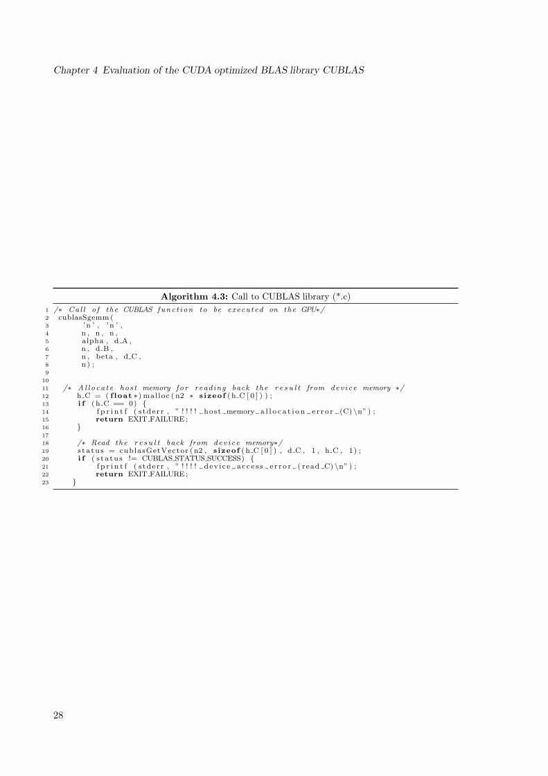
The next step is to call the CUBLAS routine and to invoke the kernel. Lines 1 to 8 ofalgorithm 4.3 show the call of the CUBLAS library function, which is similar to the call ofthe Intel MKL library; only the major storage definition is missing because of the abovementioned convention. Line 3 defines that no transposed matrices are used. Again n is takenfor every dimension as we are using square matrices. The arrays are named d A, d B andd C as this memory resides on the device. After successful execution the data is copied backto a new location seen in the lines 18 to 23 which is allocated for the results within lines 11to 16. The CUBLAS library provides currently no adjustment of the number of blocks or
25
Chapter 4 Evaluation of the CUDA optimized BLAS library CUBLAS
0
0,2
0,4
0,6
0,8
1
1,2
1,4
4 16 64 192
320
448
576
704
832
960
1088
1216
1344
1472
1600
1728
1856
1984
2112
2240
2368
2496
2624
2752
2880
3008
3136
3264
Matrix Size
GFL
OPS
/s
Figure 4.1: Performance of vanilla CPU sgemm implementation
threads per block.To complete the benchmark a simple implementation of sgemm for CUDA was taken from thenVIDIA SDK examples [9] and was integrated into the benchmark. The core functionalitycan be seen in algorithm A.5 and A.6. For better readability the important sections of theheader file, defining the blocking dimensions and the kernel call are presented together. Itwas further modified to do exactly the same calculations as the other implementations.
4.4 Results of the BLAS libraries
The performance of the CPU is not satisfactory, either in the cache or for data sets in the mainmemory as seen in figure 4.1. The performance drop which starts with matrices of order 576, ismost likely due to the cache usage of the kernel, as matrices of this size need already about 3.80MB of the 4 MB cache. Since the benchmark runs multiple times, the data must be reloadedeach time. Further performance losses are at a matrix size of 1000 elements and presumablymatrix B can no longer be held in the cache. In straight forward implementations one does notmake use of sophisticated optimization techniques e.g. blocking. Thus, this implementationmakes no use of the algorithmic low balance as the elements of matrix B must be loadedseveral times. This makes the vanilla CPU version memory bound again. More elaboratedblocking techniques need to be implemented to get a reasonable low balance. The potential ofthese advanced techniques is shown by the Intel MKL as seen in the chart 4.2. The optimizedimplementation provided by the Intel MKL library boosts the CPU performance to about 17GFLOPS/s which is maintained nearly constantly after some small spikes at the low orders.To demonstrate the performance of all cores of the host using the OpenMP capabilities of the
26
4.4 Results of the BLAS libraries
0
20
40
60
80
100
120
140
16 32 192
384
576
768
960
1152
1344
1536
1728
1920
2112
2304
2496
2688
2880
3072
3264
3456
3648
3840
4032
4224
Matrix Size
GFL
OPS
/s
Vanilla CPU Vanilla GPU Cublas GPUIntel MKL 10.0.13 one core CPU Intel MKL 10.0.13 one socket CPU Intel MKL 10.0.13 two sockets CPU
Figure 4.2: Performance of different sgemm implementations
Intel MKL, values for 4 and 8 cores, i.e. 4 and 8 threads, are presented. Four threads pinned toone socket of the workstation provide 65 GFLOPS/s. Utilizing 8 cores on two sockets leads toa performance of 125 GFLOPS/s. The performance of the vanilla CPU based implementationis even too small to fit into the scale. It was expected that the GPU platform delivers muchhigher performance than available on any CPU today. The vanilla implementation on GPUsshows good performance at nearly constant 52 GFLOPS/s per second which is more thanthree times faster than the optimized Intel MKL performance on the CPU with one core andslightly worse than one socket. The real potential available from the GPU is revealed if welook at the performance of the CUBLAS version. After the startup phase, well known fromvector based processors, the performance stays constant at 120 GFLOPs per second. Goingto the largest possible matrices on the GPU, the performance peaks up to about 250 and309 GFLOPS/s, which is then 6 times faster than a vanilla CUDA implementation and 2.5times faster than the best shown CPU version using Intel MKL. For better readability, thescale was adjusted to not show these values. The maximum performance is close to the peakperformance of the GPU which leads to speculations that there is room for improvement inthe library to achieve this performance at all feasible matrix sizes. The peaks have beenverified and are consistent over several test runs and test environments and are subject offurther investigations.
27
Chapter 4 Evaluation of the CUDA optimized BLAS library CUBLAS
Algorithm 4.3: Call to CUBLAS library (*.c)1 /∗ Cal l o f the CUBLAS func t ion to be executed on the GPU∗/2 cublasSgemm (3 ’ n ’ , ’ n ’ ,4 n , n , n ,5 alpha , d A ,6 n , d B ,7 n , beta , d C ,8 n) ;9
10
11 /∗ Al l o ca t e hos t memory fo r reading back the r e s u l t from dev i ce memory ∗/12 h C = ( f loat ∗) mal loc ( n2 ∗ s izeof ( h C [ 0 ] ) ) ;13 i f ( h C == 0) {14 f p r i n t f ( s tde r r , ” ! ! ! ! host memory a l l o c a t i o n e r r o r (C) \n” ) ;15 return EXIT FAILURE ;16 }17
18 /∗ Read the r e s u l t back from dev i ce memory∗/19 s t a t u s = cublasGetVector ( n2 , s izeof ( h C [ 0 ] ) , d C , 1 , h C , 1) ;20 i f ( s t a t u s != CUBLAS STATUS SUCCESS) {21 f p r i n t f ( s tde r r , ” ! ! ! ! dev i c e a c c e s s e r r o r ( read C) \n” ) ;22 return EXIT FAILURE ;23 }
28
Chapter 5
Porting a 3D lattice Boltzmann flow solver onthe GPU
5.1 A brief summary of the lattice Boltzmann method
In this thesis the lattice Boltzmann method is used to implement a flow solver on a GPU.In contrast to well known Navier-Stokes based flow solvers, the lattice Boltzmann methoddoes not solve a large system of non-linear partial-differential equations for the macroscopicquantities (i.e. velocity and pressure) but models the flow using a simplified kinetic approachderived from the Boltzmann equation. Starting point for the lattice Boltzmann model usedin this thesis is the Boltzmann equation with approximated collision operator according tothe simplified kinetic description of Bhatnagar, Gross, and Krook [17]:
∂tf + ~ξ · ∇f = − 1λ
[f − f (0)
](5.1)
with the distribution function f(~x, ~ξ, t), the Maxwell–Boltzmann equilibrium distributionfunction f (0), the microscopic velocity ~ξ, and the relaxation time λ. To end up with anefficient numerical approach suited for digital computers, this equation is first discretized inthe velocity space (i.e. equation 5.1 is only evaluated for few discrete velocities, so calledcollocation points). Then, spatial and temporal derivatives are replaced by (first order up-wind) finite differences and an explicit Euler time step. The result is a small set of explicitequations, called the lattice Boltzmann equations.
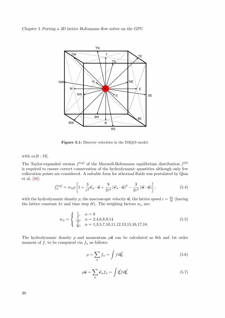
For both, accuracy and stability, the D3Q19 model first proposed by Qian et al. [30], waschosen as physical discretization of the microscopic velocity space. The resulting unit cellwith the considered microscopic velocities can be seen in figure 5.1. The discrete set ofmicroscopic velocities ~eα is defined as follows:
~eα =
(0,0,0), α = 0(±1,0,0)c,(0,±1,0)c,(0,0,±1)c, α = 2,4,6,8,9,14(±1,±1,0)c,(0,±1,±1)c,(±1, 0 ,±1)c, α = 1,3,5,7,10,11,12,13,15,16,17,18
(5.2)
Using f(~x, ~ξ, t)→ fα(~x, t), f (0)(ρ, ~ξ, ~u)→ f(eq)α (ρ, ~u), λ→ τ and ~ξ → ~eα the fully discretized
lattice Boltzmann equation reads as:
fα( ~xi + ~eαδt, t+ δt) = fα( ~xi, t)−1τ
[fα(~xi, t)− f (eq)
α (ρ, ~u)]
(5.3)
29
Chapter 5 Porting a 3D lattice Boltzmann flow solver on the GPU
N NE
C E
SES
BE
BS
B
BN
BW
SW
W
NW
TE
TN
T
TS
TW
Figure 5.1: Discrete velocities in the D3Q19 model.
with αε[0 : 18].
The Taylor-expanded version f (eq) of the Maxwell-Boltzmann equilibrium distribution f (0)
is required to ensure correct conservation of the hydrodynamic quantities although only fewcollocation points are considered. A suitable form for athermal fluids was postulated by Qianet al. [30]:
f (eq)α = wαρ
[1 +
3c2~eα · ~u+
92c4
(~eα · ~u)2 − 32c2
(~u · ~u)], (5.4)
with the hydrodynamic density ρ, the macroscopic velocity ~u, the lattice speed c = δxδt (having
the lattice constant δx and time step δt). The weighing factors wα are:
wα =
13 , α = 0118 , α = 2,4,6,8,9,14136 , α = 1,3,5,7,10,11,12,13,15,16,17,18.
(5.5)
The hydrodynamic density ρ and momentum ρ~u can be calculated as 0th and 1st ordermoment of f , to be computed via fα as follows:
ρ =∑α
fα =∫fd~ξ, (5.6)
ρ~u =∑α
~eαfα =∫~ξfd~ξ. (5.7)
30
5.2 Program hierarchy and structure
The equation of state of an ideal gas defines the pressure as p = ρc2s where cs = 1√
3c is the
sound-propagation velocity of the model. The kinematic viscosity of the fluid is given by:
ν =16
(2τ − 1)δx2
δt. (5.8)
One can think of equation 5.3 being split into two parts:
collision step: (local updates) fα(~xi, t) = fα(~xi, t)−1τ
[fα(~xi, t)− f (eq)
α (ρ, ~u)], (5.9)
streaming step: (data movement) fα(~xi + ~eαδt, t+ δt) = fα(~xi, t). (5.10)
which leads to the collide–stream order or push-method as described by Iglberger [23], withthe distribution function after the collision step fα. This splitting is only done for betterreadability but should be given up again in implementations for performance reasons as willbe shown later on.
Equation 5.3 is applied to all lattice cells of the fluid domain. Therefore first the macroscopicquantities, the velocities ~u and the density ρ, are calculated using equations 5.6 and 5.7.Next the equilibrium distribution (Equation 5.4) is calculated and the collision is performed.After that the propagation updates the data in surrounding lattice cells. For obstacle cells, aspecial treatment is applied afterwards. The third kind of cells are acceleration cells, whichare treated with an additional step, depending on the kind of acceleration.
No-slip wall boundary conditionFor the treatment of obstacles the halfway bounce-back boundary condition as described byLadd [24,25] was originally chosen, which is based on the formula:
fα(~xf , t+ δt) = fα(~xf , t), (5.11)
where ~xf is a fluid cell next to an obstacle, α is the discrete velocity direction pointing intothe solid, α is the correspondent opposite direction. So the halfway bounce-back boundarycondition reverses the momentum of a particle distribution if this distribution points towardsan obstacle.
Similar to the halfway bounce-back the fullway bounce-back is based on the formula:
fα(~xf , t+ δt) = fα(~xf , t− δt), (5.12)
The fullway bounce-back reverses the propagated value in the next timestep. This boundarycondition has advantages for the performance as will be shown later on.
5.2 Program hierarchy and structure
The implementation of the lattice Boltzmann method can be divided into two separate parts.The first prepares the lattice for the CPU and GPU kernels, the second controls the executionof the different kernels. As the CPU kernel was only used for checking correctness, details
31
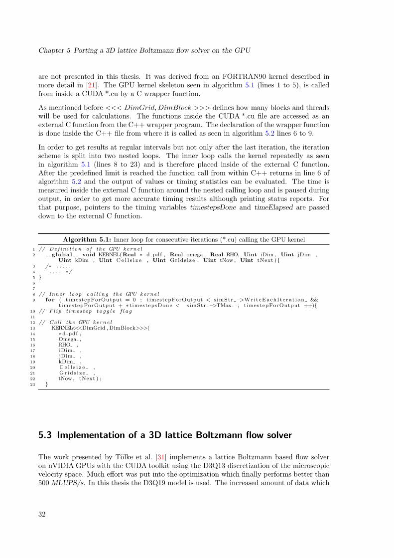
Chapter 5 Porting a 3D lattice Boltzmann flow solver on the GPU
are not presented in this thesis. It was derived from an FORTRAN90 kernel described inmore detail in [21]. The GPU kernel skeleton seen in algorithm 5.1 (lines 1 to 5), is calledfrom inside a CUDA *.cu by a C wrapper function.
As mentioned before <<< DimGrid,DimBlock >>> defines how many blocks and threadswill be used for calculations. The functions inside the CUDA *.cu file are accessed as anexternal C function from the C++ wrapper program. The declaration of the wrapper functionis done inside the C++ file from where it is called as seen in algorithm 5.2 lines 6 to 9.
In order to get results at regular intervals but not only after the last iteration, the iterationscheme is split into two nested loops. The inner loop calls the kernel repeatedly as seenin algorithm 5.1 (lines 8 to 23) and is therefore placed inside of the external C function.After the predefined limit is reached the function call from within C++ returns in line 6 ofalgorithm 5.2 and the output of values or timing statistics can be evaluated. The time ismeasured inside the external C function around the nested calling loop and is paused duringoutput, in order to get more accurate timing results although printing status reports. Forthat purpose, pointers to the timing variables timestepsDone and timeElapsed are passeddown to the external C function.
Algorithm 5.1: Inner loop for consecutive iterations (*.cu) calling the GPU kernel1 // De f i n i t i on o f the GPU kerne l2 global void KERNEL(Real ∗ d pdf , Real omega , Real RHO, Uint iDim , Uint jDim ,
Uint kDim , Uint C e l l s i z e , Uint Grids i ze , Uint tNow , Uint tNext ) {3 /∗ . . . . .4 . . . . ∗/5 }6
7
8 // Inner loop c a l l i n g the GPU kerne l9 for ( timestepForOutput = 0 ; timestepForOutput < s imStr −>WriteEachI te ra t ion &&
timestepForOutput + ∗ t imestepsDone < s imStr −>TMax ; timestepForOutput ++){10 // F l ip t imes tep t o g g l e f l a g11
12 // Ca l l the GPU kerne l13 KERNEL<<<DimGrid , DimBlock>>>(14 ∗d pdf ,15 Omega ,16 RHO ,17 iDim ,18 jDim ,19 kDim ,20 C e l l s i z e ,21 G r i d s i z e ,22 tNow , tNext ) ;23 }
5.3 Implementation of a 3D lattice Boltzmann flow solver
The work presented by Tolke et al. [31] implements a lattice Boltzmann based flow solveron nVIDIA GPUs with the CUDA toolkit using the D3Q13 discretization of the microscopicvelocity space. Much effort was put into the optimization which finally performs better than500 MLUPS/s. In this thesis the D3Q19 model is used. The increased amount of data which
32
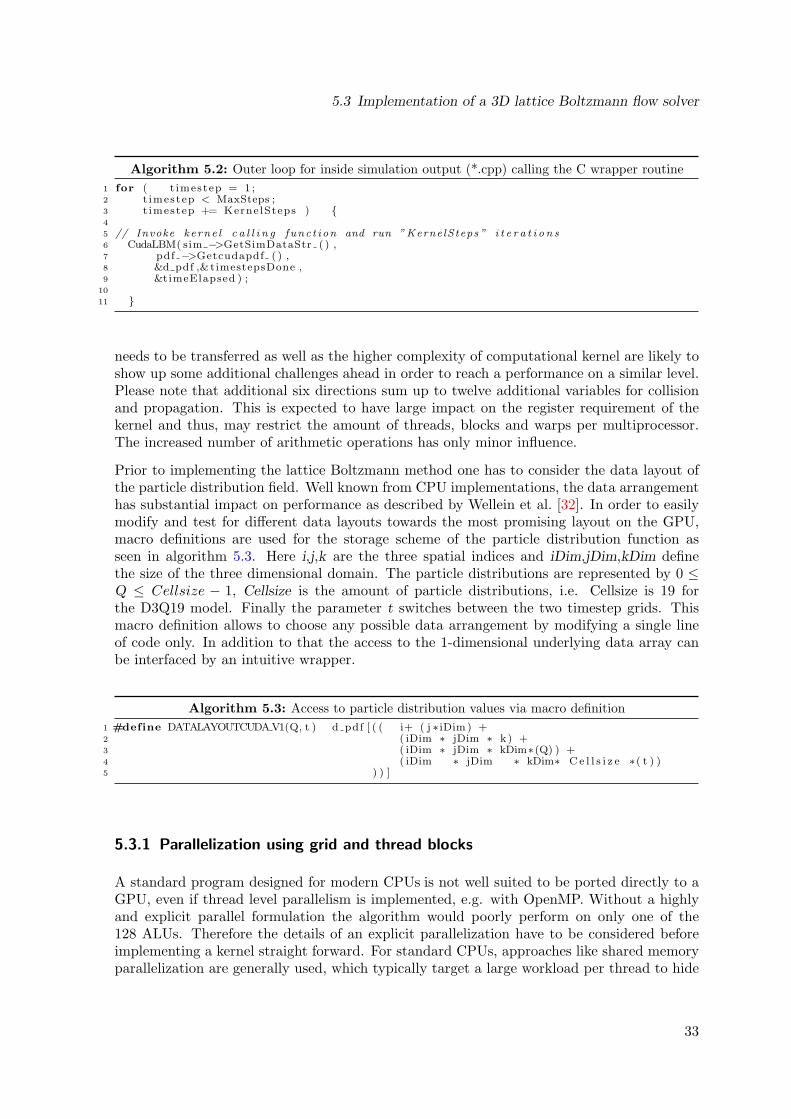
5.3 Implementation of a 3D lattice Boltzmann flow solver
Algorithm 5.2: Outer loop for inside simulation output (*.cpp) calling the C wrapper routine1 for ( t imestep = 1 ;2 t imestep < MaxSteps ;3 t imestep += KernelSteps ) {4
5 // Invoke ke rne l c a l l i n g func t i on and run ”KernelSteps ” i t e r a t i o n s6 CudaLBM( sim −>GetSimDataStr ( ) ,7 pdf −>Getcudapdf ( ) ,8 &d pdf ,& timestepsDone ,9 &timeElapsed ) ;
10
11 }
needs to be transferred as well as the higher complexity of computational kernel are likely toshow up some additional challenges ahead in order to reach a performance on a similar level.Please note that additional six directions sum up to twelve additional variables for collisionand propagation. This is expected to have large impact on the register requirement of thekernel and thus, may restrict the amount of threads, blocks and warps per multiprocessor.The increased number of arithmetic operations has only minor influence.
Prior to implementing the lattice Boltzmann method one has to consider the data layout ofthe particle distribution field. Well known from CPU implementations, the data arrangementhas substantial impact on performance as described by Wellein et al. [32]. In order to easilymodify and test for different data layouts towards the most promising layout on the GPU,macro definitions are used for the storage scheme of the particle distribution function asseen in algorithm 5.3. Here i,j,k are the three spatial indices and iDim,jDim,kDim definethe size of the three dimensional domain. The particle distributions are represented by 0 ≤Q ≤ Cellsize − 1, Cellsize is the amount of particle distributions, i.e. Cellsize is 19 forthe D3Q19 model. Finally the parameter t switches between the two timestep grids. Thismacro definition allows to choose any possible data arrangement by modifying a single lineof code only. In addition to that the access to the 1-dimensional underlying data array canbe interfaced by an intuitive wrapper.
Algorithm 5.3: Access to particle distribution values via macro definition1 #define DATALAYOUTCUDA V1(Q, t ) d pdf [ ( ( i+ ( j ∗ iDim ) +2 ( iDim ∗ jDim ∗ k ) +3 ( iDim ∗ jDim ∗ kDim∗(Q) ) +4 ( iDim ∗ jDim ∗ kDim∗ C e l l s i z e ∗( t ) )5 ) ) ]
5.3.1 Parallelization using grid and thread blocks
A standard program designed for modern CPUs is not well suited to be ported directly to aGPU, even if thread level parallelism is implemented, e.g. with OpenMP. Without a highlyand explicit parallel formulation the algorithm would poorly perform on only one of the128 ALUs. Therefore the details of an explicit parallelization have to be considered beforeimplementing a kernel straight forward. For standard CPUs, approaches like shared memoryparallelization are generally used, which typically target a large workload per thread to hide
33

Chapter 5 Porting a 3D lattice Boltzmann flow solver on the GPU
Thread 0 Thread 1 Thread 2
0 ... 18 0 ... 18 0 ... 18
0 0 0Offset of 19 elements
Offset of 19 elements
... ... ...
First load
Figure 5.2: Wrongly aligned distribution of elements to threads with array-of-structures
Thread 0 Thread 1 Thread 2
0 0 0 ... ... ... 18 18 18
0 0 0Aligned memory
load
Aligned memory
load
... ... ...
First load
Figure 5.3: Correctly aligned distribution of elements to threads with structure-of-arrays layout
34
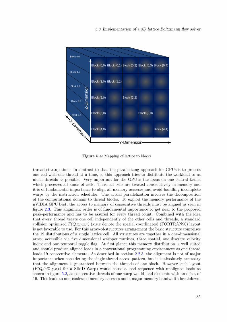
5.3 Implementation of a 3D lattice Boltzmann flow solver
Block (4,4)
Block (3,3)
Block (4,0)
Block (3,0)
Block (2,2)
Block (1,1)
Block (2,0)
Block (1,0)
Block (0,4)Block (0,3)Block (0,2)Block (0,1)Block (0,0)
Block 0,0
Block 1,0
Block 2,0
Block 3,0
Block 4,0
Y-Dimension
X-Dimension
Z-D
imen
sion
Figure 5.4: Mapping of lattice to blocks
thread startup time. In contrast to that the parallelizing approach for GPUs is to processone cell with one thread at a time, so this approach tries to distribute the workload to asmuch threads as possible. Very important for the GPU is the focus on one central kernelwhich processes all kinds of cells. Thus, all cells are treated consecutively in memory andit is of fundamental importance to align all memory accesses and avoid handling incompletewarps by the instruction scheduler. The actual parallelization involves the decompositionof the computational domain to thread blocks. To exploit the memory performance of thenVIDIA GPU best, the access to memory of consecutive threads must be aligned as seen infigure 2.3. This alignment order is of fundamental importance to get near to the proposedpeak-performance and has to be assured for every thread count. Combined with the ideathat every thread treats one cell independently of the other cells and threads, a standardcollision optimized F(Q,x,y,z,t) (x,y,z denote the spatial coordinates) (FORTRAN90) layoutis not favorable to use. For this array-of-structures arrangement the basic structure comprisesthe 19 distributions of a single lattice cell. All structures are together in a one-dimensionalarray, accessible via five dimensional wrapper routines, three spatial, one discrete velocityindex and one temporal toggle flag. At first glance this memory distribution is well suitedand should produce aligned loads in a conventional programming environment as one threadloads 19 consecutive elements. As described in section 2.2.3, the alignment is not of majorimportance when considering the single thread access pattern, but it is absolutely necessarythat the alignment is guaranteed between the threads of one block. However such layout(F(Q,0:31,y,z,t) for a SIMD-Warp) would cause a load sequence with unaligned loads asshown in figure 5.2, as consecutive threads of one warp would load elements with an offset of19. This leads to non-coalesced memory accesses and a major memory bandwidth breakdown.
35
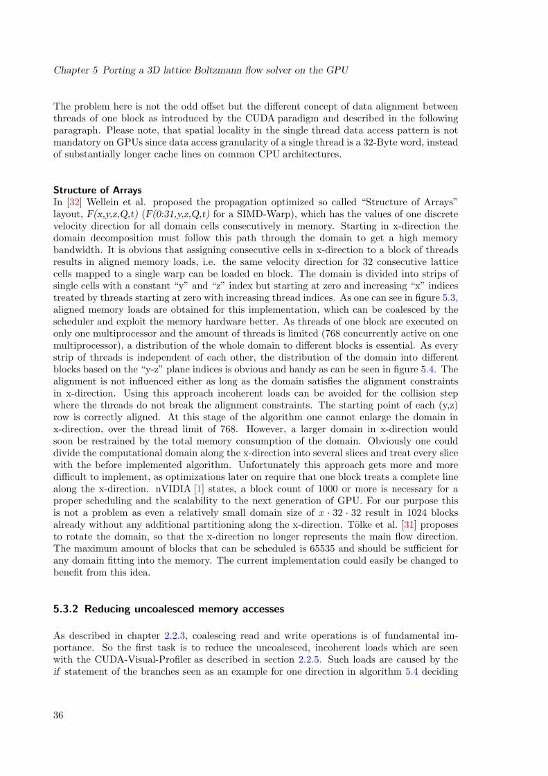
Chapter 5 Porting a 3D lattice Boltzmann flow solver on the GPU
The problem here is not the odd offset but the different concept of data alignment betweenthreads of one block as introduced by the CUDA paradigm and described in the followingparagraph. Please note, that spatial locality in the single thread data access pattern is notmandatory on GPUs since data access granularity of a single thread is a 32-Byte word, insteadof substantially longer cache lines on common CPU architectures.
Structure of ArraysIn [32] Wellein et al. proposed the propagation optimized so called “Structure of Arrays”layout, F(x,y,z,Q,t) (F(0:31,y,z,Q,t) for a SIMD-Warp), which has the values of one discretevelocity direction for all domain cells consecutively in memory. Starting in x-direction thedomain decomposition must follow this path through the domain to get a high memorybandwidth. It is obvious that assigning consecutive cells in x-direction to a block of threadsresults in aligned memory loads, i.e. the same velocity direction for 32 consecutive latticecells mapped to a single warp can be loaded en block. The domain is divided into strips ofsingle cells with a constant “y” and “z” index but starting at zero and increasing “x” indicestreated by threads starting at zero with increasing thread indices. As one can see in figure 5.3,aligned memory loads are obtained for this implementation, which can be coalesced by thescheduler and exploit the memory hardware better. As threads of one block are executed ononly one multiprocessor and the amount of threads is limited (768 concurrently active on onemultiprocessor), a distribution of the whole domain to different blocks is essential. As everystrip of threads is independent of each other, the distribution of the domain into differentblocks based on the “y-z” plane indices is obvious and handy as can be seen in figure 5.4. Thealignment is not influenced either as long as the domain satisfies the alignment constraintsin x-direction. Using this approach incoherent loads can be avoided for the collision stepwhere the threads do not break the alignment constraints. The starting point of each (y,z)row is correctly aligned. At this stage of the algorithm one cannot enlarge the domain inx-direction, over the thread limit of 768. However, a larger domain in x-direction wouldsoon be restrained by the total memory consumption of the domain. Obviously one coulddivide the computational domain along the x-direction into several slices and treat every slicewith the before implemented algorithm. Unfortunately this approach gets more and moredifficult to implement, as optimizations later on require that one block treats a complete linealong the x-direction. nVIDIA [1] states, a block count of 1000 or more is necessary for aproper scheduling and the scalability to the next generation of GPU. For our purpose thisis not a problem as even a relatively small domain size of x · 32 · 32 result in 1024 blocksalready without any additional partitioning along the x-direction. Tolke et al. [31] proposesto rotate the domain, so that the x-direction no longer represents the main flow direction.The maximum amount of blocks that can be scheduled is 65535 and should be sufficient forany domain fitting into the memory. The current implementation could easily be changed tobenefit from this idea.
5.3.2 Reducing uncoalesced memory accesses
As described in chapter 2.2.3, coalescing read and write operations is of fundamental im-portance. So the first task is to reduce the uncoalesced, incoherent loads which are seenwith the CUDA-Visual-Profiler as described in section 2.2.5. Such loads are caused by theif statement of the branches seen as an example for one direction in algorithm 5.4 deciding
36
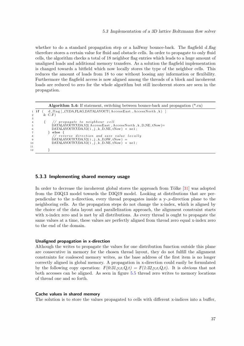
5.3 Implementation of a 3D lattice Boltzmann flow solver
whether to do a standard propagation step or a halfway bounce-back. The flagfield d flagtherefore stores a certain value for fluid and obstacle cells. In order to propagate to only fluidcells, the algorithm checks a total of 18 neighbor flag entries which leads to a huge amount ofunaligned loads and additional memory transfers. As a solution the flagfield implementationis changed towards a bitfield which now locally stores the type of the neighbor cells. Thisreduces the amount of loads from 18 to one without loosing any information or flexibility.Furthermore the flagfield access is now aligned among the threads of a block and incoherentloads are reduced to zero for the whole algorithm but still incoherent stores are seen in thepropagation.
Algorithm 5.4: If statement, switching between bounce-back and propagation (*.cu)1 i f ( d f l a g [ CUDA FLAG DATALAYOUT( AccessEast , AccessNorth , k ) ]2 & C F)3
4 { // propagate to neighbour c e l l5 DATALAYOUTCUDA V2( AccessEast , AccessNorth , k ,D NE, tNow)=6 DATALAYOUTCUDA V2( i , j , k ,D NE, tNow) ∗ ne1 ;7 } else {8 // reve r se d i r e c t i on and save va lue l o c a l l y9 DATALAYOUTCUDA V2( i , j , k ,D SW, tNow) =
10 DATALAYOUTCUDA V2( i , j , k ,D NE, tNow) ∗ ne1 ;11
12 }
5.3.3 Implementing shared memory usage
In order to decrease the incoherent global stores the approach from Tolke [31] was adoptedfrom the D3Q13 model towards the D3Q19 model. Looking at distributions that are per-pendicular to the x-direction, every thread propagates inside a y-,z-direction plane to theneighboring cells. As the propagation steps do not change the x-index, which is aligned bythe choice of the data layout and parallelization approach, the alignment constraint startswith x-index zero and is met by all distributions. As every thread is ought to propagate thesame values at a time, these values are perfectly aligned from thread zero equal x-index zeroto the end of the domain.
Unaligned propagation in x-directionAlthough the writes to propagate the values for one distribution function outside this planeare consecutive in memory for the chosen thread layout, they do not fulfill the alignmentconstraints for coalesced memory writes, as the base address of the first item is no longercorrectly aligned in global memory. A propagation in x-direction could easily be formulatedby the following copy operation: F(0:31,y,z,Q,t) = F(1:32,y,z,Q,t). It is obvious that notboth accesses can be aligned. As seen in figure 5.5 thread zero writes to memory locationsof thread one and so forth.
Cache values in shared memoryThe solution is to store the values propagated to cells with different x-indices into a buffer,
37
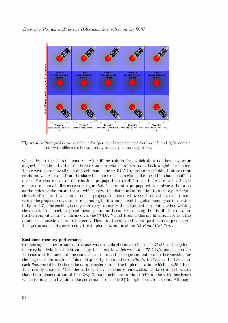
Chapter 5 Porting a 3D lattice Boltzmann flow solver on the GPU
Thread 2propagating and
storing
Thread 1propagating and
storing
Thread 0propagating and
storing
Thread 3propagating and
storing
Thread 4propagating and
storing
Thread 0: Write to BaseAdress +
1
Base
add
ress
mee
ts a
lignm
ent c
onst
rain
ts
Thread 2: Write to BaseAdress +
2
Thread 3: Write to BaseAdress +
3
Thread 3: Write to BaseAdress +
4
Thread 4: Write to BaseAdress +
0
Thread
4
Link 1
0
Thread 0
Link 15
Thread 1
Link 15
Thread 2
Link 15
Thread 3
Link 15
Thread 4
Link 15
Thread
0Lin
k 10
Thread
1
Link 1
0
Thread
2
Link 1
0
Thread
3
Link 1
0
Figure 5.5: Propagation to neighbor cells (periodic boundary condition on left and right domainend) with different x-index, leading to unaligned memory stores.
which lies in the shared memory. After filling this buffer, which does not have to occuraligned, each thread writes the buffer contents related to its x-index back to global memory.These writes are now aligned and coherent. The nVIDIA Programming Guide [1] states thatreads and writes to and from the shared memory reach a register-like speed if no bank conflictsoccur. For that reason all distributions propagating to a different x-index are cached insidea shared memory buffer as seen in figure 5.6. The x-index propagated to is always the sameas the index of the future thread which stores the distribution function to memory. After allthreads of a block have completed the propagation, ensured by synchronization, each threadwrites the propagated values corresponding to its x-index back to global memory as illustratedin figure 5.7. The caching is only necessary to satisfy the alignment constraints when writingthe distributions back to global memory and not because of reusing the distribution data forfurther computations. Confirmed via the CUDA-Visual-Profiler this modification reduced thenumber of uncoalesced stores to zero. Therefore the optimal access pattern is implemented.The performance obtained using this implementation is about 53 FluidMLUPS/s .
Sustained memory performanceComparing this performance, testcase was a standard domain of size 64x32x32, to the gainedmemory bandwidth of the Streamcopy benchmark, which was about 75 GB/s, one has to take19 loads and 19 stores into account for collision and propagation and one further variable forthe flag field information. This multiplied by the number of FluidMLUPS/s and 4 Bytes foreach float variable, leads to the data transfer rate of the implementation which is 8.26 GB/s.This is only about 11 % of the earlier achieved memory bandwidth. Tolke et al. [31] statesthat the implementation of the D3Q13 model achieves to about 54% of the GPU hardwarewhich is more than five times the performance of the D3Q19 implementation, so far. Although
38
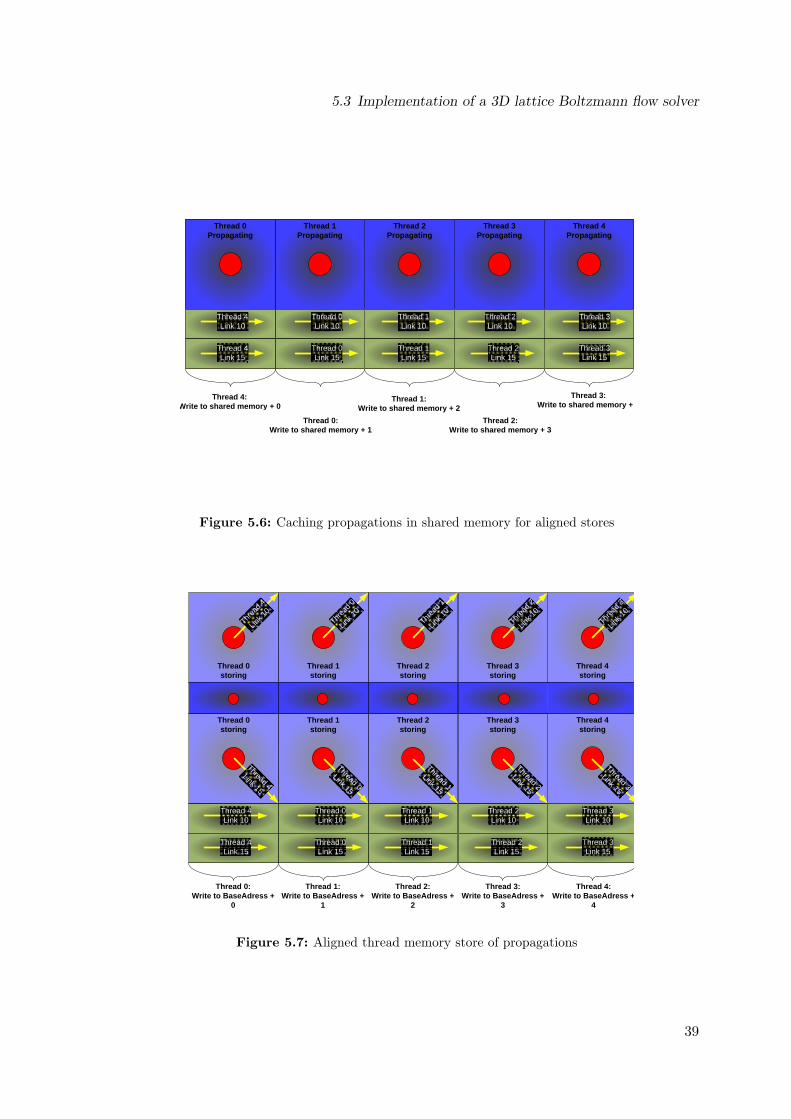
5.3 Implementation of a 3D lattice Boltzmann flow solver
Thread 2Propagating
Thread 1Propagating
Thread 0Propagating
Thread 3Propagating
Thread 4Propagating
Thread 4: Write to shared memory + 0
Thread 0: Write to shared memory + 1
Thread 1: Write to shared memory + 2
Thread 2: Write to shared memory + 3
Thread 3: Write to shared memory +
Thread 4 Link 10
Thread 0Link 10
Thread 1 Link 10
Thread 2 Link 10
Thread 3 Link 10
Thread 2 Link 15
Thread 3 Link 15
Thread 0 Link 15
Thread 1 Link 15
Thread 4 Link 15
Figure 5.6: Caching propagations in shared memory for aligned stores
Thread 4 Link 10
Thread 0Link 10
Thread 1 Link 10
Thread 2 Link 10
Thread 3 Link 10
Thread 2 Link 15
Thread 3 Link 15
Thread 0 Link 15
Thread 1 Link 15
Thread 4 Link 15
Thread 0: Write to BaseAdress +
0
Thread 1: Write to BaseAdress +
1
Thread 2: Write to BaseAdress +
2
Thread 3: Write to BaseAdress +
3
Thread 4: Write to BaseAdress +
4
Thread 2storing
Thread 1storing
Thread 0storing
Thread 3storing
Thread 4storing
Thread 2storing
Thread 1storing
Thread 0storing
Thread 3storing
Thread 4storing
Thread
4
Link 1
0
Thread 0
Link 15
Thread 1
Link 15
Thread 2
Link 15
Thread 3
Link 15
Thread 4
Link 15
Thread
0Lin
k 10
Thread
1
Link 1
0
Thread
2
Link 1
0
Thread
3
Link 1
0
Figure 5.7: Aligned thread memory store of propagations
39
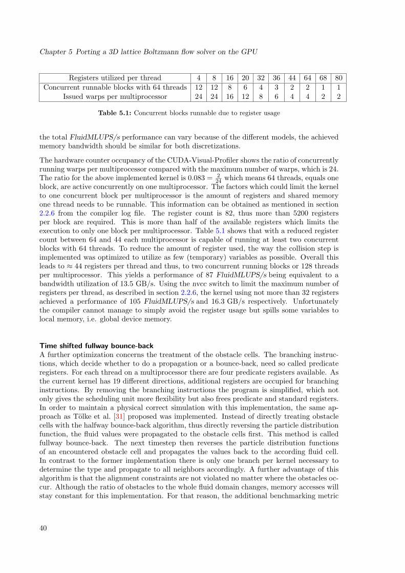
Chapter 5 Porting a 3D lattice Boltzmann flow solver on the GPU
Registers utilized per thread 4 8 16 20 32 36 44 64 68 80Concurrent runnable blocks with 64 threads 12 12 8 6 4 3 2 2 1 1
Issued warps per multiprocessor 24 24 16 12 8 6 4 4 2 2
Table 5.1: Concurrent blocks runnable due to register usage
the total FluidMLUPS/s performance can vary because of the different models, the achievedmemory bandwidth should be similar for both discretizations.
The hardware counter occupancy of the CUDA-Visual-Profiler shows the ratio of concurrentlyrunning warps per multiprocessor compared with the maximum number of warps, which is 24.The ratio for the above implemented kernel is 0.083 = 2
24 which means 64 threads, equals oneblock, are active concurrently on one multiprocessor. The factors which could limit the kernelto one concurrent block per multiprocessor is the amount of registers and shared memoryone thread needs to be runnable. This information can be obtained as mentioned in section2.2.6 from the compiler log file. The register count is 82, thus more than 5200 registersper block are required. This is more than half of the available registers which limits theexecution to only one block per multiprocessor. Table 5.1 shows that with a reduced registercount between 64 and 44 each multiprocessor is capable of running at least two concurrentblocks with 64 threads. To reduce the amount of register used, the way the collision step isimplemented was optimized to utilize as few (temporary) variables as possible. Overall thisleads to ≈ 44 registers per thread and thus, to two concurrent running blocks or 128 threadsper multiprocessor. This yields a performance of 87 FluidMLUPS/s being equivalent to abandwidth utilization of 13.5 GB/s. Using the nvcc switch to limit the maximum number ofregisters per thread, as described in section 2.2.6, the kernel using not more than 32 registersachieved a performance of 105 FluidMLUPS/s and 16.3 GB/s respectively. Unfortunatelythe compiler cannot manage to simply avoid the register usage but spills some variables tolocal memory, i.e. global device memory.
Time shifted fullway bounce-backA further optimization concerns the treatment of the obstacle cells. The branching instruc-tions, which decide whether to do a propagation or a bounce-back, need so called predicateregisters. For each thread on a multiprocessor there are four predicate registers available. Asthe current kernel has 19 different directions, additional registers are occupied for branchinginstructions. By removing the branching instructions the program is simplified, which notonly gives the scheduling unit more flexibility but also frees predicate and standard registers.In order to maintain a physical correct simulation with this implementation, the same ap-proach as Tolke et al. [31] proposed was implemented. Instead of directly treating obstaclecells with the halfway bounce-back algorithm, thus directly reversing the particle distributionfunction, the fluid values were propagated to the obstacle cells first. This method is calledfullway bounce-back. The next timestep then reverses the particle distribution functionsof an encountered obstacle cell and propagates the values back to the according fluid cell.In contrast to the former implementation there is only one branch per kernel necessary todetermine the type and propagate to all neighbors accordingly. A further advantage of thisalgorithm is that the alignment constraints are not violated no matter where the obstacles oc-cur. Although the ratio of obstacles to the whole fluid domain changes, memory accesses willstay constant for this implementation. For that reason, the additional benchmarking metric
40
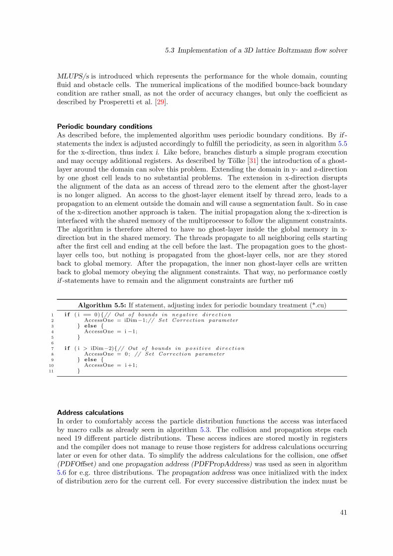
5.3 Implementation of a 3D lattice Boltzmann flow solver
MLUPS/s is introduced which represents the performance for the whole domain, countingfluid and obstacle cells. The numerical implications of the modified bounce-back boundarycondition are rather small, as not the order of accuracy changes, but only the coefficient asdescribed by Prosperetti et al. [29].
Periodic boundary conditionsAs described before, the implemented algorithm uses periodic boundary conditions. By if -statements the index is adjusted accordingly to fulfill the periodicity, as seen in algorithm 5.5for the x-direction, thus index i. Like before, branches disturb a simple program executionand may occupy additional registers. As described by Tolke [31] the introduction of a ghost-layer around the domain can solve this problem. Extending the domain in y- and z-directionby one ghost cell leads to no substantial problems. The extension in x-direction disruptsthe alignment of the data as an access of thread zero to the element after the ghost-layeris no longer aligned. An access to the ghost-layer element itself by thread zero, leads to apropagation to an element outside the domain and will cause a segmentation fault. So in caseof the x-direction another approach is taken. The initial propagation along the x-direction isinterfaced with the shared memory of the multiprocessor to follow the alignment constraints.The algorithm is therefore altered to have no ghost-layer inside the global memory in x-direction but in the shared memory. The threads propagate to all neighboring cells startingafter the first cell and ending at the cell before the last. The propagation goes to the ghost-layer cells too, but nothing is propagated from the ghost-layer cells, nor are they storedback to global memory. After the propagation, the inner non ghost-layer cells are writtenback to global memory obeying the alignment constraints. That way, no performance costlyif -statements have to remain and the alignment constraints are further m6
Algorithm 5.5: If statement, adjusting index for periodic boundary treatment (*.cu)1 i f ( i == 0) {// Out o f bounds in nega t i v e d i r e c t i on2 AccessOne = iDim−1;// Set Correct ion parameter3 } else {4 AccessOne = i −1;5 }6
7 i f ( i > iDim−2){// Out o f bounds in p o s i t i v e d i r e c t i on8 AccessOne = 0 ; // Set Correct ion parameter9 } else {
10 AccessOne = i +1;11 }
Address calculationsIn order to comfortably access the particle distribution functions the access was interfacedby macro calls as already seen in algorithm 5.3. The collision and propagation steps eachneed 19 different particle distributions. These access indices are stored mostly in registersand the compiler does not manage to reuse those registers for address calculations occurringlater or even for other data. To simplify the address calculations for the collision, one offset(PDFOffset) and one propagation address (PDFPropAddress) was used as seen in algorithm5.6 for e.g. three distributions. The propagation address was once initialized with the indexof distribution zero for the current cell. For every successive distribution the index must be
41
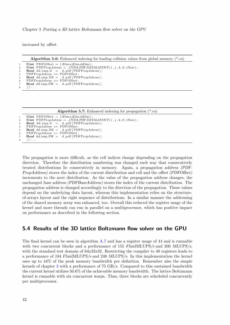
Chapter 5 Porting a 3D lattice Boltzmann flow solver on the GPU
increased by offset.
Algorithm 5.6: Enhanced indexing for loading collision values from global memory (*.cu)1 Uint PDFOffset = ( iDim∗ jDim∗kDim) ;2 Uint PDFPropAdress = CUDA PDF DATALAYOUT( i , j , k , 0 , tNow) ;3 Real dd tmp 0 = d pdf [ PDFPropAdress ] ;4 PDFPropAdress += PDFOffset ;5 Real dd tmp NE = d pdf [ PDFPropAdress ] ;6 PDFPropAdress += PDFOffset ;7 Real dd tmp SW = d pdf [ PDFPropAdress ] ;8 // . . .
Algorithm 5.7: Enhanced indexing for propagation (*.cu)1 Uint PDFOffset = ( iDim∗ jDim∗kDim) ;2 Uint PDFPropAdress = CUDA PDF DATALAYOUT( i , j , k , 0 , tNow) ;3 Real dd tmp 0 = d pdf [ PDFPropAdress ] ;4 PDFPropAdress += PDFOffset ;5 Real dd tmp NE = d pdf [ PDFPropAdress ] ;6 PDFPropAdress += PDFOffset ;7 Real dd tmp SW = d pdf [ PDFPropAdress ] ;8 // . . .
The propagation is more difficult, as the cell indices change depending on the propagationdirection. Therefore the distribution numbering was changed such way that consecutivelytreated distributions lie consecutively in memory. Again, a propagation address (PDF-PropAddress) stores the index of the current distribution and cell and the offset (PDFOffset)increments to the next distribution. As the value of the propagation address changes, theunchanged base address (PDFBaseAddress) stores the index of the current distribution. Thepropagation address is changed accordingly to the direction of the propagation. These valuesdepend on the underlying data layout, whereas this implementation relies on the structure-of-arrays layout and the right sequence of distributions. In a similar manner the addressingof the shared memory array was enhanced, too. Overall this reduced the register usage of thekernel and more threads can run in parallel on a multiprocessor, which has positive impacton performance as described in the following section.
5.4 Results of the 3D lattice Boltzmann flow solver on the GPU
The final kernel can be seen in algorithm A.7 and has a register usage of 44 and is runnablewith two concurrent blocks and a performance of 155 FluidMLUPS/s and 200 MLUPS/s,with the standard test domain of 64x32x32. Restricting the compiler to 40 registers leads toa performance of 184 FluidMLUPS/s and 248 MLUPS/s. In this implementation the kerneluses up to 44% of the peak memory bandwidth per definition. Remember also the simplekernels of chapter 3 with a performance of 75 GB/s. Compared to this sustained bandwidththe current kernel utilizes 50.6% of the achievable memory bandwidth. The lattice Boltzmannkernel is runnable with six concurrent warps. Thus, three blocks are scheduled concurrentlyper multiprocessor.
42
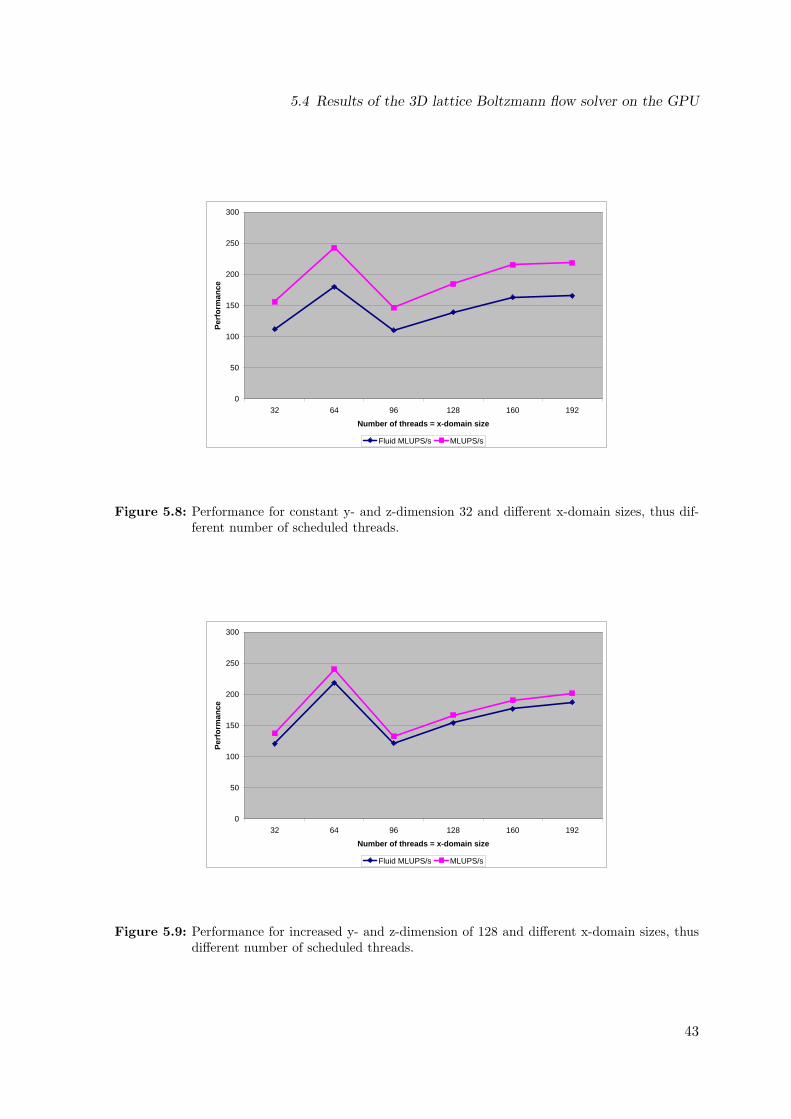
5.4 Results of the 3D lattice Boltzmann flow solver on the GPU
0
50
100
150
200
250
300
32 64 96 128 160 192
Number of threads = x-domain size
Perf
orm
ance
Fluid MLUPS/s MLUPS/s
Figure 5.8: Performance for constant y- and z-dimension 32 and different x-domain sizes, thus dif-ferent number of scheduled threads.
0
50
100
150
200
250
300
32 64 96 128 160 192
Number of threads = x-domain size
Perf
orm
ance
Fluid MLUPS/s MLUPS/s
Figure 5.9: Performance for increased y- and z-dimension of 128 and different x-domain sizes, thusdifferent number of scheduled threads.
43
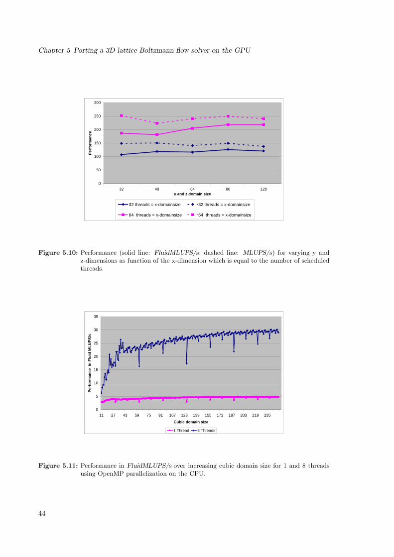
Chapter 5 Porting a 3D lattice Boltzmann flow solver on the GPU
0
50
100
150
200
250
300
32 48 64 80 128y and z domain size
Perf
orm
ance
32 threads = x-domainsize 32 threads = x-domainsize
64 threads = x-domainsize 64 threads = x-domainsize
Figure 5.10: Performance (solid line: FluidMLUPS/s; dashed line: MLUPS/s) for varying y andz-dimensions as function of the x-dimension which is equal to the number of scheduledthreads.
0
5
10
15
20
25
30
35
11 27 43 59 75 91 107 123 139 155 171 187 203 219 235
Cubic domain size
Perf
orm
ance
in
Flui
d M
LUPS
/s
1 Thread 8 Threads
Figure 5.11: Performance in FluidMLUPS/s over increasing cubic domain size for 1 and 8 threadsusing OpenMP parallelization on the CPU.
44
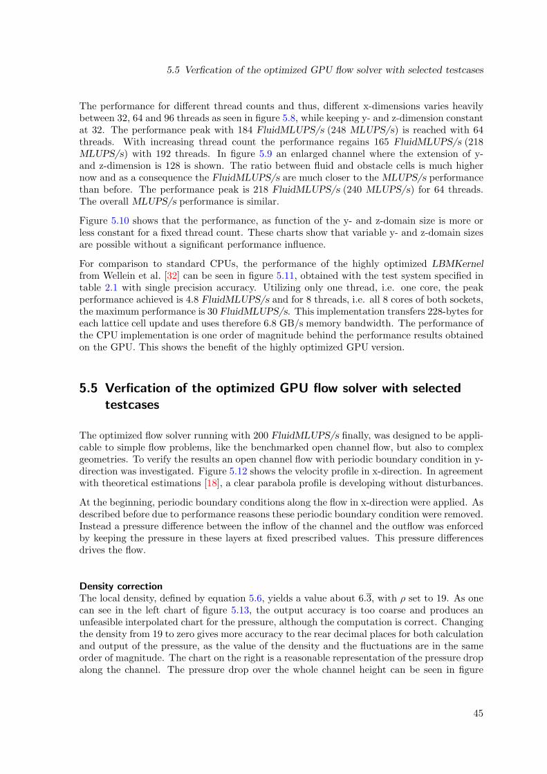
5.5 Verfication of the optimized GPU flow solver with selected testcases
The performance for different thread counts and thus, different x-dimensions varies heavilybetween 32, 64 and 96 threads as seen in figure 5.8, while keeping y- and z-dimension constantat 32. The performance peak with 184 FluidMLUPS/s (248 MLUPS/s) is reached with 64threads. With increasing thread count the performance regains 165 FluidMLUPS/s (218MLUPS/s) with 192 threads. In figure 5.9 an enlarged channel where the extension of y-and z-dimension is 128 is shown. The ratio between fluid and obstacle cells is much highernow and as a consequence the FluidMLUPS/s are much closer to the MLUPS/s performancethan before. The performance peak is 218 FluidMLUPS/s (240 MLUPS/s) for 64 threads.The overall MLUPS/s performance is similar.
Figure 5.10 shows that the performance, as function of the y- and z-domain size is more orless constant for a fixed thread count. These charts show that variable y- and z-domain sizesare possible without a significant performance influence.
For comparison to standard CPUs, the performance of the highly optimized LBMKernelfrom Wellein et al. [32] can be seen in figure 5.11, obtained with the test system specified intable 2.1 with single precision accuracy. Utilizing only one thread, i.e. one core, the peakperformance achieved is 4.8 FluidMLUPS/s and for 8 threads, i.e. all 8 cores of both sockets,the maximum performance is 30 FluidMLUPS/s. This implementation transfers 228-bytes foreach lattice cell update and uses therefore 6.8 GB/s memory bandwidth. The performance ofthe CPU implementation is one order of magnitude behind the performance results obtainedon the GPU. This shows the benefit of the highly optimized GPU version.
5.5 Verfication of the optimized GPU flow solver with selectedtestcases
The optimized flow solver running with 200 FluidMLUPS/s finally, was designed to be appli-cable to simple flow problems, like the benchmarked open channel flow, but also to complexgeometries. To verify the results an open channel flow with periodic boundary condition in y-direction was investigated. Figure 5.12 shows the velocity profile in x-direction. In agreementwith theoretical estimations [18], a clear parabola profile is developing without disturbances.
At the beginning, periodic boundary conditions along the flow in x-direction were applied. Asdescribed before due to performance reasons these periodic boundary condition were removed.Instead a pressure difference between the inflow of the channel and the outflow was enforcedby keeping the pressure in these layers at fixed prescribed values. This pressure differencesdrives the flow.
Density correctionThe local density, defined by equation 5.6, yields a value about 6.3, with ρ set to 19. As onecan see in the left chart of figure 5.13, the output accuracy is too coarse and produces anunfeasible interpolated chart for the pressure, although the computation is correct. Changingthe density from 19 to zero gives more accuracy to the rear decimal places for both calculationand output of the pressure, as the value of the density and the fluctuations are in the sameorder of magnitude. The chart on the right is a reasonable representation of the pressure dropalong the channel. The pressure drop over the whole channel height can be seen in figure
45
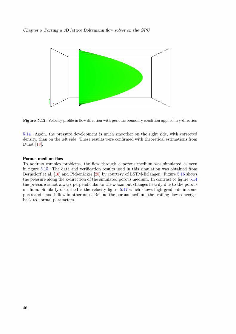
Chapter 5 Porting a 3D lattice Boltzmann flow solver on the GPU
Figure 5.12: Velocity profile in flow direction with periodic boundary condition applied in y-direction
5.14. Again, the pressure development is much smoother on the right side, with correcteddensity, than on the left side. These results were confirmed with theoretical estimations fromDurst [18].
Porous medium flowTo address complex problems, the flow through a porous medium was simulated as seenin figure 5.15. The data and verification results used in this simulation was obtained fromBernsdorf et al. [16] and Pickenacker [28] by courtesy of LSTM-Erlangen. Figure 5.16 showsthe pressure along the x-direction of the simulated porous medium. In contrast to figure 5.14the pressure is not always perpendicular to the x-axis but changes heavily due to the porousmedium. Similarly disturbed is the velocity figure 5.17 which shows high gradients in somepores and smooth flow in other ones. Behind the porous medium, the trailing flow convergesback to normal parameters.
46
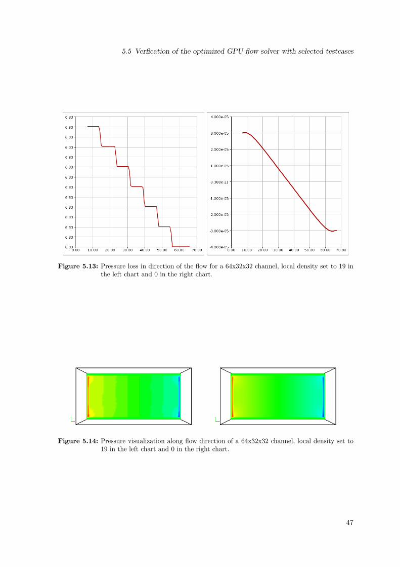
5.5 Verfication of the optimized GPU flow solver with selected testcases
Figure 5.13: Pressure loss in direction of the flow for a 64x32x32 channel, local density set to 19 inthe left chart and 0 in the right chart.
Figure 5.14: Pressure visualization along flow direction of a 64x32x32 channel, local density set to19 in the left chart and 0 in the right chart.
47
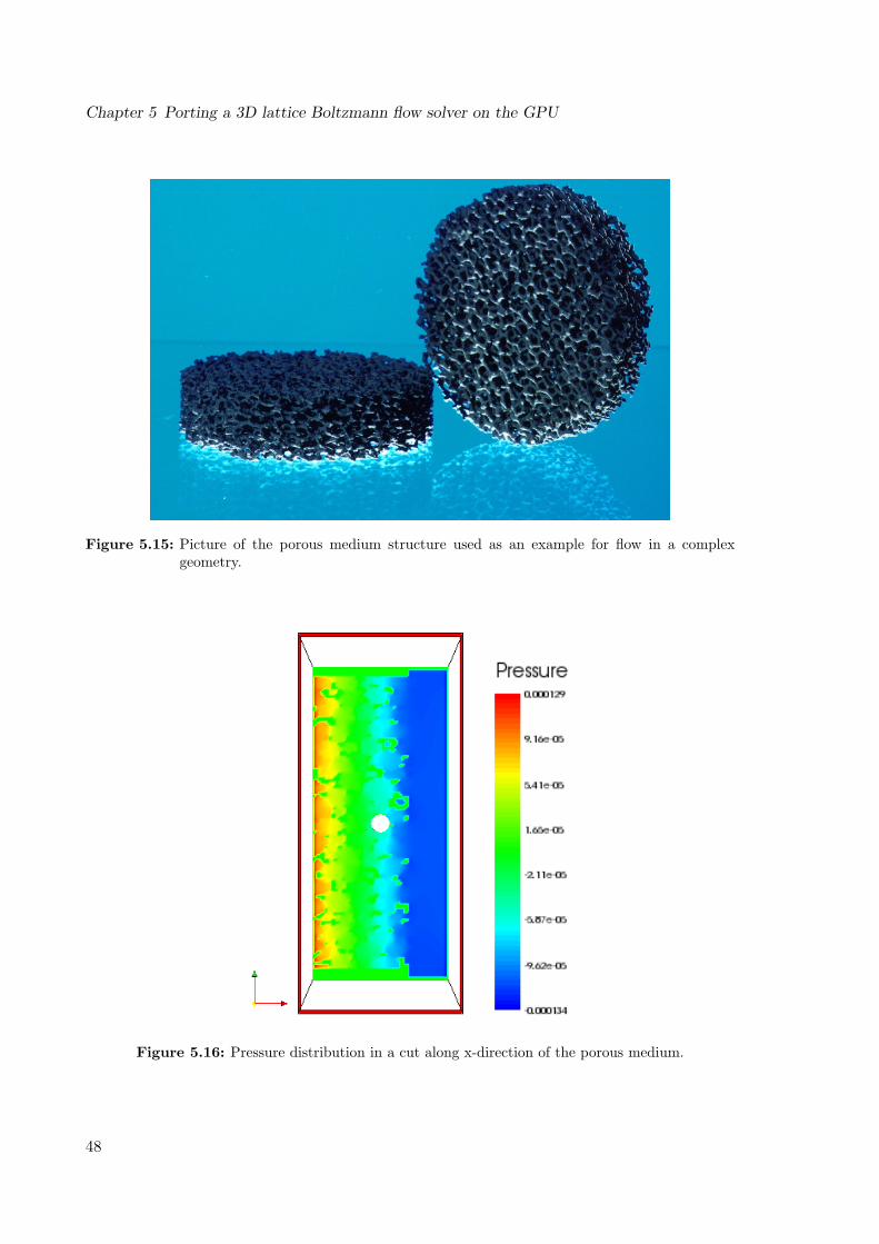
Chapter 5 Porting a 3D lattice Boltzmann flow solver on the GPU
Figure 5.15: Picture of the porous medium structure used as an example for flow in a complexgeometry.
Figure 5.16: Pressure distribution in a cut along x-direction of the porous medium.
48
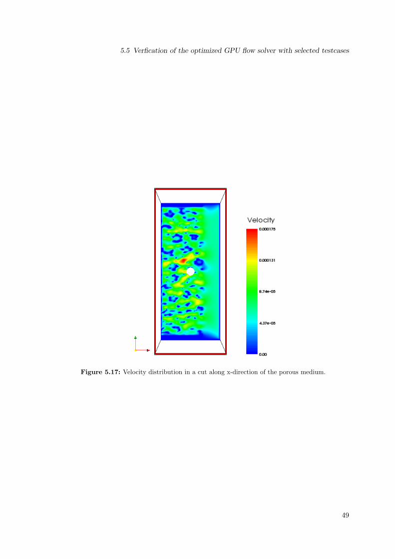
5.5 Verfication of the optimized GPU flow solver with selected testcases
Figure 5.17: Velocity distribution in a cut along x-direction of the porous medium.
49
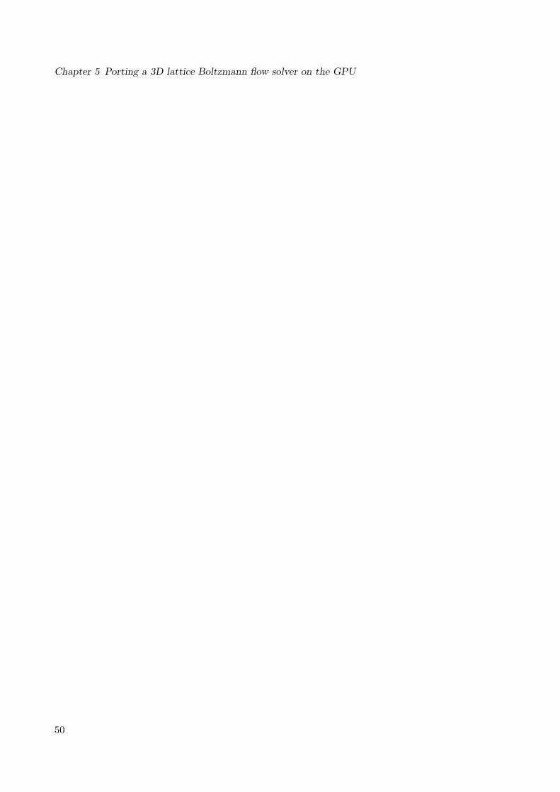
Chapter 5 Porting a 3D lattice Boltzmann flow solver on the GPU
50
Chapter 6
Conclusion
The topics analyzed in this thesis are performance characteristics and efficient programmingstyles of the nVIDIA G80 GPU, as well as parallelization techniques for the Compute UnifiedDevice Architecture. As compared to standard multi-core CPUs the memory hierarchy iscompletely different. Classical cache levels are missing completely. But there are two differentkinds of memory, the extremely small local on-chip memory and high-latency, high-bandwidthdevice memory. The concept of GPUs, which use SIMD style, hides data access latency andlatency of pipeline units by utilizing massive parallelism on the thread level. To hide dataaccesses efficiently, data must be aligned in memory and threads have to load and store datacoherently. Moreover, hardware resources in terms of register and local on-chip memorycan put very strict limits on the maximum number of threads, running concurrently. Sincethis might limit the latency hiding efforts, low level optimizations are therefore crucial foradvanced algorithms. Addressing those problems in terms of performance optimizations, a farmore detailed code analysis must be performed, e.g. minimizing if-branches can substantiallyimprove performance because of reduced register usage due to predicating instructions. As thealignment and distribution of data is largely unimportant in programming common standardCPU hardware the main challenge is to distribute the accesses to the elements in the globalmemory of the GPU correctly, so that the full bandwidth is utilized. The step from the simpleSTREAM benchmark kernels to the more sophisticated lattice Boltzmann kernel showed aneven increased complexity in both read and write alignment. As no alignment constraintsexist for the shared memory it is mainly used to reorder unaligned memory accesses in sucha way that device memory access is finally aligned. Therefore it was mainly an interfacebetween the registers and the memory. Thus, this additional memory hierarchy does not actas a cache but as a reorder buffer
The performance of numerical operations has been the primary focus of this thesis and there-fore simple kernels like the STREAM benchmark were implemented first, then the GPUimplementation of a BLAS routine was evaluated and finally a fluid flow solver was imple-mented and highly optimized. The results are positive throughout the given scenarios. Theapplications showed that both, the arithmetic and memory bandwidth peak performancescan be reached and sustained. For simple kernels like those of the STREAM benchmark ahuge performance gain can be achieved with little effort. This demonstrates that the pro-gramming paradigm and the implementation is applicable in general. A memory bandwidthof 85%, i.e. 75 GB/s of 86.4 GB/s, could be sustained. Common CPU platforms typicallyachieve 50% or even less of the peak memory bandwidth. In multi-socket environments thesustainable performance can be even lower due to cache coherence protocol overhead.
The basic use of the GPU implementation of the BLAS library, called CUBLAS, is not as
51
Chapter 6 Conclusion
simple as with well-established libraries, because the memory on the GPU must be allocatedmanually. The implementation of the sgemm BLAS routine on nVIDIA GPUs shows similarperformance to common dual-socket quad-core servers. However, the performance is onlyabout 34% of the proposed arithmetic peak performance which might be interpreted suchthat the implementation is still immature. At some problem sizes however, the performancemore than doubles and reaches 309 GFLOPS/s which is about 90% of the peak performanceof the GPU. So there seems to be room for improvement in future releases of the CUBLASlibrary.
For more complex code structures like the flow solver based on the lattice Boltzmann kernelabout ten times the performance of current architectures, e.g. dual-socket quad-core servers,could be achieved. The algorithm utilized 45% of the memory peak performance and 50%of the achievable memory bandwidth, as measured by the STREAM benchmark. The efforthowever, for implementing was tremendous, as various changes of the fundamental algorithmwere necessary as well as sophisticated optimizations, based on the analysis of assembler codeand application of performance analysis tools. The major problems that occurred were dueto the branches in the program, unaligned loads and stores and overall register usage whichlimited the amount of thread parallelism on one multiprocessor.
In general, every algorithm which is memory bound should be considered to be ported toGPUs as long as it is highly parallelizable. Considerations about the complexity of a kernelare another criterion. Simple kernels should not be a problem as the thread level parallelismshould not be affected. The more complex a kernel the more difficult it is to obtain the sus-tainable memory performance as register usage limits the number of concurrently scheduledthreads. A kernel which is bound by the arithmetic performance of the hardware and has alow memory footprint, i.e. most data can be kept in local memory, should show massive per-formance improvements, as current GPUs provide more than 350 GFLOPS/s in comparisonto about 100 GFLOPS/s per quad core CPU chip. This high GPU performance still comesat the cost that numerical accuracy is restricted to single precision.
Future research should investigate the opportunities of advanced register saving techniquesas well as assembler coded addenda to enhance the register usage of compiled algorithms.Exemplary functions of the CUBLAS library should be analyzed to find the problems of thecurrent implementation and to provide fast alternatives, which are adoptable to increasingshared memory and register sizes and multiprocessor counts. A topic not covered until nowis the bandwidth between GPU global memory and the host system memory. With the ideaof fast GPUs comes the idea of fast GPU clusters which need to communicate with the hostsystem and with other nodes via the PCI-E bus. This will address transfer optimizations ofthe hardware as well as improved models of domain decomposition and synchronization. Thenext generation of GPUs, with doubled arithmetic performance and a memory bandwidthgain of at least one third, will increase the parallelism available on GPUs. The supportfor calculations in double precision will be natively implemented, however, at the cost ofsubstantial performance loss.
Porting algorithms and programs to GPUs should be a long-term commitment as interop-erability between different hardware vendors is not in sight. Development toolkits, such asRAPIDMIND [14], that combine CPU, GPU and other promising architectures, e.g. theCell Broadband Engine are a glimpse of a potential future development direction in scien-tific computing on accelerators and are not mature yet. Although the programming effort
52
is much higher compared to serial algorithm development, future performance enhancementswill no longer be achieved by faster serial execution, but with higher parallelism. Thereforeprogramming GPUs, such as nVIDIA series with CUDA might already give a first view onfuture optimization and parallelization techniques for standard CPUs addressing issues, likehigh on-chip parallelism and efficient use of rare shared on-chip resources.
53

Chapter 6 Conclusion
54
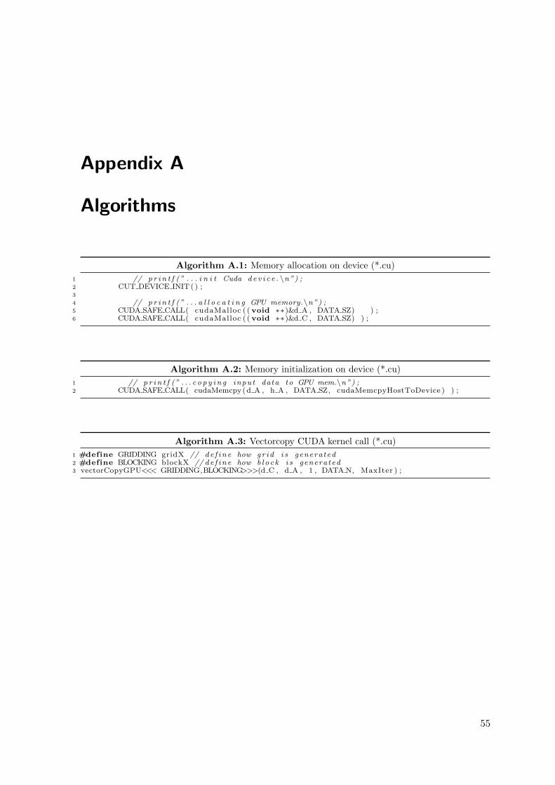
Appendix A
Algorithms
Algorithm A.1: Memory allocation on device (*.cu)1 // p r i n t f (” . . . i n i t Cuda d e v i c e . \n”) ;2 CUT DEVICE INIT( ) ;3
4 // p r i n t f (” . . . a l l o c a t i n g GPU memory.\n”) ;5 CUDA SAFE CALL( cudaMalloc ( ( void ∗∗)&d A , DATA SZ) ) ;6 CUDA SAFE CALL( cudaMalloc ( ( void ∗∗)&d C , DATA SZ) ) ;
Algorithm A.2: Memory initialization on device (*.cu)1 // p r i n t f (” . . . c o p y i n g input data to GPU mem.\n”) ;2 CUDA SAFE CALL( cudaMemcpy(d A , h A , DATA SZ, cudaMemcpyHostToDevice ) ) ;
Algorithm A.3: Vectorcopy CUDA kernel call (*.cu)1 #define GRIDDING gridX // de f ine how gr i d i s generated2 #define BLOCKING blockX // de f ine how b l o ck i s generated3 vectorCopyGPU<<< GRIDDING,BLOCKING>>>(d C , d A , 1 , DATA N, MaxIter ) ;
55
Appendix A Algorithms
Algorithm A.4: nVIDIA SDK disclaimer.1 /∗2 ∗ Copyright 1993−2007 NVIDIA Corporat ion. A l l r i g h t s r e s e r v ed .3 ∗4 ∗ NOTICE TO USER:5 ∗6 ∗ This source code i s s u b j e c t to NVIDIA ownership r i g h t s under U.S. and7 ∗ i n t e r na t i ona l Copyright l aws . Users and pos s e s so r s o f t h i s source code8 ∗ are hereby granted a nonexc lus ive , roya l t y−f r e e l i c e n s e to use t h i s code9 ∗ in i n d i v i d u a l and commercial s o f twa r e .
10 ∗11 ∗ NVIDIA MAKES NO REPRESENTATION ABOUT THE SUITABILITY OF THIS SOURCE12 ∗ CODE FOR ANY PURPOSE. IT IS PROVIDED ”AS IS” WITHOUT EXPRESS OR13 ∗ IMPLIED WARRANTY OF ANY KIND. NVIDIA DISCLAIMS ALL WARRANTIES WITH14 ∗ REGARD TO THIS SOURCE CODE, INCLUDING ALL IMPLIED WARRANTIES OF15 ∗ MERCHANTABILITY, NONINFRINGEMENT, AND FITNESS FOR A PARTICULAR PURPOSE.16 ∗ IN NO EVENT SHALL NVIDIA BE LIABLE FOR ANY SPECIAL, INDIRECT, INCIDENTAL,17 ∗ OR CONSEQUENTIAL DAMAGES, OR ANY DAMAGES WHATSOEVER RESULTING FROM LOSS18 ∗ OF USE, DATA OR PROFITS, WHETHER IN AN ACTION OF CONTRACT, NEGLIGENCE19 ∗ OR OTHER TORTIOUS ACTION, ARISING OUT OF OR IN CONNECTION WITH THE USE20 ∗ OR PERFORMANCE OF THIS SOURCE CODE.21 ∗22 ∗ U.S. Government End Users . This source code i s a ”commercial item” as23 ∗ t ha t term i s de f ined at 48 C.F.R. 2 .101 (OCT 1995) , c on s i s t i n g o f24 ∗ ”commercial computer so f tware ” and ”commercial computer so f tware25 ∗ documentation” as such terms are used in 48 C.F.R. 12 .212 (SEPT 1995)26 ∗ and i s prov ided to the U.S. Government only as a commercial end i tem.27 ∗ Cons is tent with 48 C.F.R.12.212 and 48 C.F.R. 227 .7202−1 through28 ∗ 227 .7202−4 (JUNE 1995) , a l l U.S. Government End Users acqu i re the29 ∗ source code with only those r i g h t s s e t f o r t h he r e i n .30 ∗31 ∗ Any use o f t h i s source code in i n d i v i d u a l and commercial so f tware must32 ∗ inc lude , in the user documentation and i n t e r na l comments to the code ,33 ∗ the above Disc la imer and U.S. Government End Users Not i ce .34 ∗/
56
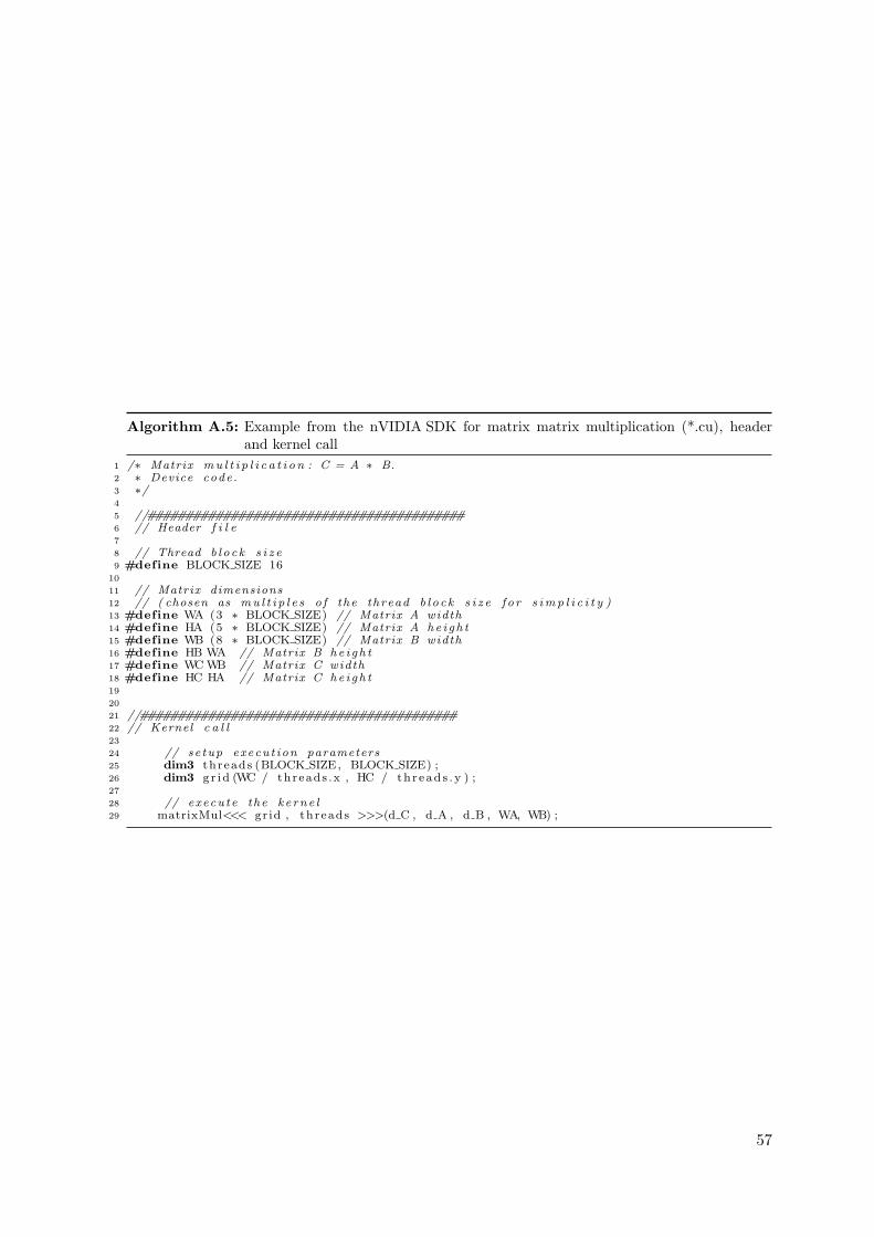
Algorithm A.5: Example from the nVIDIA SDK for matrix matrix multiplication (*.cu), headerand kernel call
1 /∗ Matrix mu l t i p l i c a t i o n : C = A ∗ B.2 ∗ Device code .3 ∗/4
5 //##########################################6 // Header f i l e7
8 // Thread b l o c k s i z e9 #define BLOCK SIZE 16
10
11 // Matrix dimensions12 // ( chosen as mu l t i p l e s o f the thread b l o c k s i z e f o r s imp l i c i t y )13 #define WA (3 ∗ BLOCK SIZE) // Matrix A width14 #define HA (5 ∗ BLOCK SIZE) // Matrix A he i gh t15 #define WB (8 ∗ BLOCK SIZE) // Matrix B width16 #define HB WA // Matrix B he i gh t17 #define WC WB // Matrix C width18 #define HC HA // Matrix C he i gh t19
20
21 //##########################################22 // Kernel c a l l23
24 // se tup execu t ion parameters25 dim3 threads (BLOCK SIZE, BLOCK SIZE) ;26 dim3 g r id (WC / threads .x , HC / th r ead s . y ) ;27
28 // execute the ke rne l29 matrixMul<<< gr id , threads >>>(d C , d A , d B , WA, WB) ;
57

Appendix A Algorithms
Algorithm A.6: Example from the nVIDIA SDK for matrix matrix multiplication (*.cu), kernelimplementation
1 //##########################################2 // Kernel s e c t i on3 #include <s td i o . h>4 #include ” matrixMul.h ”5
6 ////////////////////////////////////////////////////////////////////////////////7 // ! Matrix mu l t i p l i c a t i o n on the dev i ce : C = A ∗ B8 // ! wA i s A’ s width and wB i s B ’ s width9 ////////////////////////////////////////////////////////////////////////////////
10 global void11 matrixMul ( f loat ∗ C, f loat ∗ A, f loat ∗ B, int wA, int wB)12 {13 // Block index14 int bx = block Idx .x ;15 int by = block Idx .y ;16 // Thread index17 int tx = threadIdx .x ;18 int ty = threadIdx .y ;19 // Index o f the f i r s t sub−matrix o f A processed by the b l o c k20 int aBegin = wA ∗ BLOCK SIZE ∗ by ;21 // Index o f the l a s t sub−matrix o f A processed by the b l o c k22 int aEnd = aBegin + wA − 1 ;23 // Stop s i z e used to i t e r a t e through the sub−matrices o f A24 int aStep = BLOCK SIZE ;25 // Index o f the f i r s t sub−matrix o f B processed by the b l o c k26 int bBegin = BLOCK SIZE ∗ bx ;27 // Step s i z e used to i t e r a t e through the sub−matrices o f B28 int bStep = BLOCK SIZE ∗ wB;29 // Csub i s used to s t o r e the element o f the b l o c k sub−matrix30 // tha t i s computed by the thread31 f loat Csub = 0 ;32
33 // Loop over a l l the sub−matrices o f A and B34 // requ i red to compute the b l o c k sub−matrix35 for ( int a = aBegin , b = bBegin ;36 a <= aEnd ;37 a += aStep , b += bStep ) {38 // Dec lara t ion o f the shared memory array As used to39 // s t o r e the sub−matrix o f A40 shared f loat As [ BLOCK SIZE ] [ BLOCK SIZE ] ;41 // Dec lara t ion o f the shared memory array Bs used to42 // s t o r e the sub−matrix o f B43 shared f loat Bs [ BLOCK SIZE ] [ BLOCK SIZE ] ;44 // Load the matr ices from dev i ce memory45 // to shared memory ; each thread loads46 // one element o f each matrix47 AS( ty , tx ) = A[ a + wA ∗ ty + tx ] ;48 BS( ty , tx ) = B[ b + wB ∗ ty + tx ] ;49 // Synchronize to make sure the matr ices are loaded50 sync th r ead s ( ) ;51 // Mul t i p l y the two matr ices t o g e t h e r ;52 // each thread computes one element53 // o f the b l o c k sub−matrix54 for ( int k = 0 ; k < BLOCK SIZE ; ++k )55 Csub += AS( ty , k ) ∗ BS(k , tx ) ;56 // Synchronize to make sure t ha t the preced ing57 // computation i s done be f o re l oad ing two new58 // sub−matrices o f A and B in the next i t e r a t i o n59 sync th r ead s ( ) ;60 }61 // Write the b l o c k sub−matrix to dev i ce memory ;62 // each thread wr i t e s one element63 int c = wB ∗ BLOCK SIZE ∗ by + BLOCK SIZE ∗ bx ;64 C[ c + wB ∗ ty + tx ] = Csub ;65 }
58
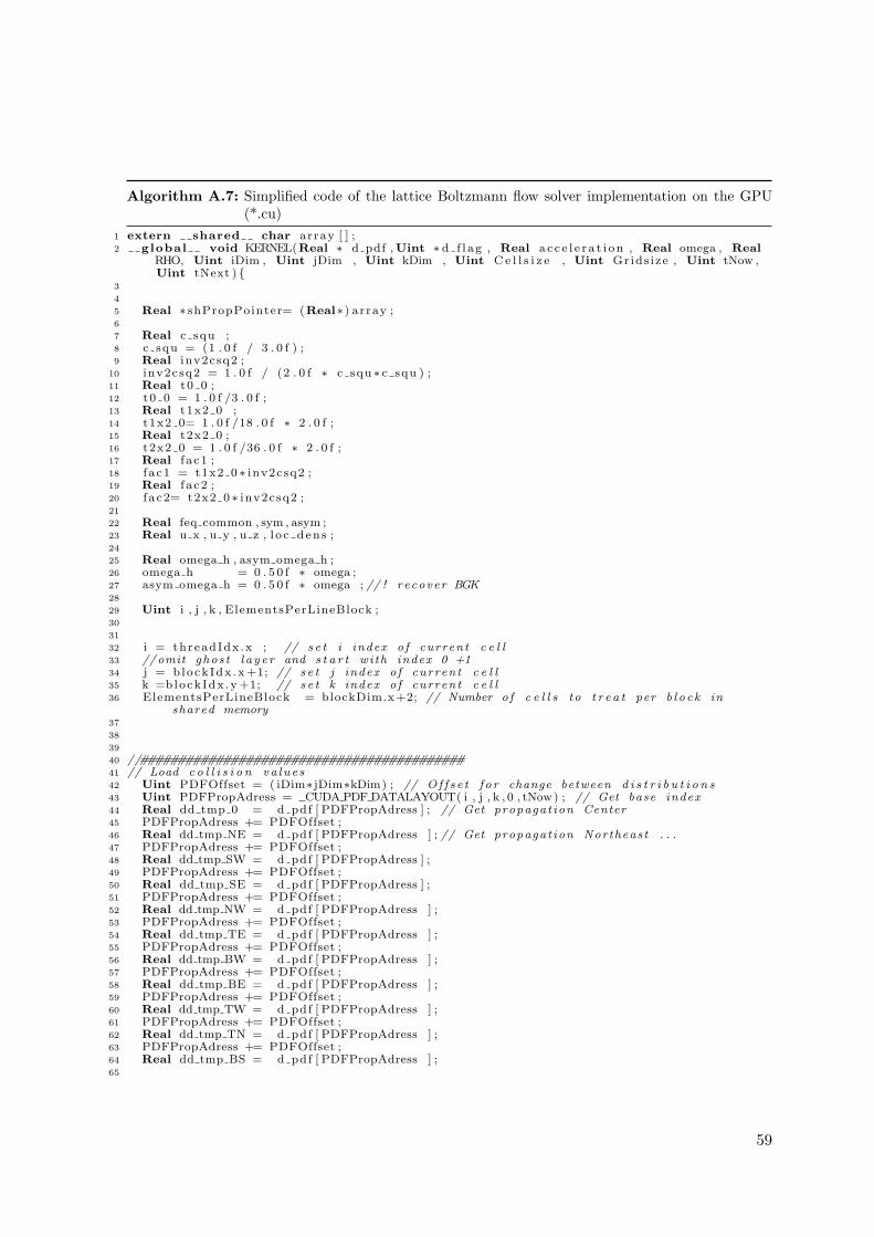
Algorithm A.7: Simplified code of the lattice Boltzmann flow solver implementation on the GPU(*.cu)
1 extern shared char array [ ] ;2 global void KERNEL(Real ∗ d pdf , Uint ∗ d f l ag , Real a c c e l e r a t i o n , Real omega , Real
RHO, Uint iDim , Uint jDim , Uint kDim , Uint C e l l s i z e , Uint Grids i ze , Uint tNow ,Uint tNext ) {
3
4
5 Real ∗ shPropPointer= (Real∗) array ;6
7 Real c squ ;8 c squ = (1 . 0 f / 3 . 0 f ) ;9 Real inv2csq2 ;
10 inv2csq2 = 1 . 0 f / (2 . 0 f ∗ c squ ∗ c squ ) ;11 Real t0 0 ;12 t0 0 = 1 . 0 f /3 . 0 f ;13 Real t1x2 0 ;14 t1x2 0= 1 . 0 f /18 . 0 f ∗ 2 . 0 f ;15 Real t2x2 0 ;16 t2x2 0 = 1 . 0 f /36 . 0 f ∗ 2 . 0 f ;17 Real f a c1 ;18 f a c1 = t1x2 0 ∗ inv2csq2 ;19 Real f a c2 ;20 f a c2= t2x2 0 ∗ inv2csq2 ;21
22 Real feq common , sym , asym ;23 Real u x , u y , u z , l o c d e n s ;24
25 Real omega h , asym omega h ;26 omega h = 0 . 5 0 f ∗ omega ;27 asym omega h = 0 . 5 0 f ∗ omega ; // ! recover BGK28
29 Uint i , j , k , ElementsPerLineBlock ;30
31
32 i = threadIdx .x ; // s e t i index o f current c e l l33 //omit ghos t l a y e r and s t a r t wi th index 0 +134 j = b lock Idx .x +1; // s e t j index o f current c e l l35 k =block Idx .y +1; // s e t k index o f current c e l l36 ElementsPerLineBlock = blockDim.x +2; // Number o f c e l l s to t r e a t per b l o c k in
shared memory37
38
39
40 //###########################################41 // Load c o l l i s i o n va lue s42 Uint PDFOffset = ( iDim∗ jDim∗kDim) ; // Of f s e t f o r change between d i s t r i b u t i o n s43 Uint PDFPropAdress = CUDA PDF DATALAYOUT( i , j , k , 0 , tNow) ; // Get base index44 Real dd tmp 0 = d pdf [ PDFPropAdress ] ; // Get propagat ion Center45 PDFPropAdress += PDFOffset ;46 Real dd tmp NE = d pdf [ PDFPropAdress ] ; // Get propagat ion Northeast . . .47 PDFPropAdress += PDFOffset ;48 Real dd tmp SW = d pdf [ PDFPropAdress ] ;49 PDFPropAdress += PDFOffset ;50 Real dd tmp SE = d pdf [ PDFPropAdress ] ;51 PDFPropAdress += PDFOffset ;52 Real dd tmp NW = d pdf [ PDFPropAdress ] ;53 PDFPropAdress += PDFOffset ;54 Real dd tmp TE = d pdf [ PDFPropAdress ] ;55 PDFPropAdress += PDFOffset ;56 Real dd tmp BW = d pdf [ PDFPropAdress ] ;57 PDFPropAdress += PDFOffset ;58 Real dd tmp BE = d pdf [ PDFPropAdress ] ;59 PDFPropAdress += PDFOffset ;60 Real dd tmp TW = d pdf [ PDFPropAdress ] ;61 PDFPropAdress += PDFOffset ;62 Real dd tmp TN = d pdf [ PDFPropAdress ] ;63 PDFPropAdress += PDFOffset ;64 Real dd tmp BS = d pdf [ PDFPropAdress ] ;65
59
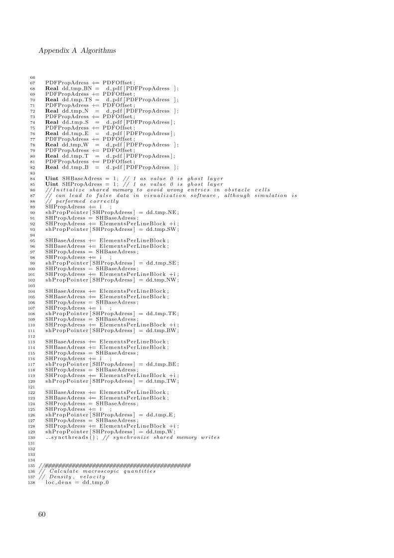
Appendix A Algorithms
66
67 PDFPropAdress += PDFOffset ;68 Real dd tmp BN = d pdf [ PDFPropAdress ] ;69 PDFPropAdress += PDFOffset ;70 Real dd tmp TS = d pdf [ PDFPropAdress ] ;71 PDFPropAdress += PDFOffset ;72 Real dd tmp N = d pdf [ PDFPropAdress ] ;73 PDFPropAdress += PDFOffset ;74 Real dd tmp S = d pdf [ PDFPropAdress ] ;75 PDFPropAdress += PDFOffset ;76 Real dd tmp E = d pdf [ PDFPropAdress ] ;77 PDFPropAdress += PDFOffset ;78 Real dd tmp W = d pdf [ PDFPropAdress ] ;79 PDFPropAdress += PDFOffset ;80 Real dd tmp T = d pdf [ PDFPropAdress ] ;81 PDFPropAdress += PDFOffset ;82 Real dd tmp B = d pdf [ PDFPropAdress ] ;83
84 Uint SHBaseAdress = 1 ; // 1 as va lue 0 i s ghos t l a y e r85 Uint SHPropAdress = 1 ; // 1 as va lue 0 i s ghos t l a y e r86 // I n i t i a l i z e shared memory to avoid wrong en t r i e s in o b s t a c l e c e l l s87 // can lead to f a l s e data in v i s u a l i z a t i o n sof tware , a l though s imu la t ion i s88 // performed c o r r e c t l y89 SHPropAdress += i ;90 shPropPointer [ SHPropAdress ] = dd tmp NE ;91 SHPropAdress = SHBaseAdress ;92 SHPropAdress += ElementsPerLineBlock +i ;93 shPropPointer [ SHPropAdress ] = dd tmp SW ;94
95 SHBaseAdress += ElementsPerLineBlock ;96 SHBaseAdress += ElementsPerLineBlock ;97 SHPropAdress = SHBaseAdress ;98 SHPropAdress += i ;99 shPropPointer [ SHPropAdress ] = dd tmp SE ;
100 SHPropAdress = SHBaseAdress ;101 SHPropAdress += ElementsPerLineBlock +i ;102 shPropPointer [ SHPropAdress ] = dd tmp NW ;103
104 SHBaseAdress += ElementsPerLineBlock ;105 SHBaseAdress += ElementsPerLineBlock ;106 SHPropAdress = SHBaseAdress ;107 SHPropAdress += i ;108 shPropPointer [ SHPropAdress ] = dd tmp TE ;109 SHPropAdress = SHBaseAdress ;110 SHPropAdress += ElementsPerLineBlock +i ;111 shPropPointer [ SHPropAdress ] = dd tmp BW ;112
113 SHBaseAdress += ElementsPerLineBlock ;114 SHBaseAdress += ElementsPerLineBlock ;115 SHPropAdress = SHBaseAdress ;116 SHPropAdress += i ;117 shPropPointer [ SHPropAdress ] = dd tmp BE ;118 SHPropAdress = SHBaseAdress ;119 SHPropAdress += ElementsPerLineBlock +i ;120 shPropPointer [ SHPropAdress ] = dd tmp TW ;121
122 SHBaseAdress += ElementsPerLineBlock ;123 SHBaseAdress += ElementsPerLineBlock ;124 SHPropAdress = SHBaseAdress ;125 SHPropAdress += i ;126 shPropPointer [ SHPropAdress ] = dd tmp E ;127 SHPropAdress = SHBaseAdress ;128 SHPropAdress += ElementsPerLineBlock +i ;129 shPropPointer [ SHPropAdress ] = dd tmp W ;130 sync th r ead s ( ) ; // synchronize shared memory wr i t e s131
132
133
134
135 //###########################################136 // Ca l cu la t e macroscopic q u an t i t i e s137 // Density , v e l o c i t y138 l o c d e n s = dd tmp 0
60
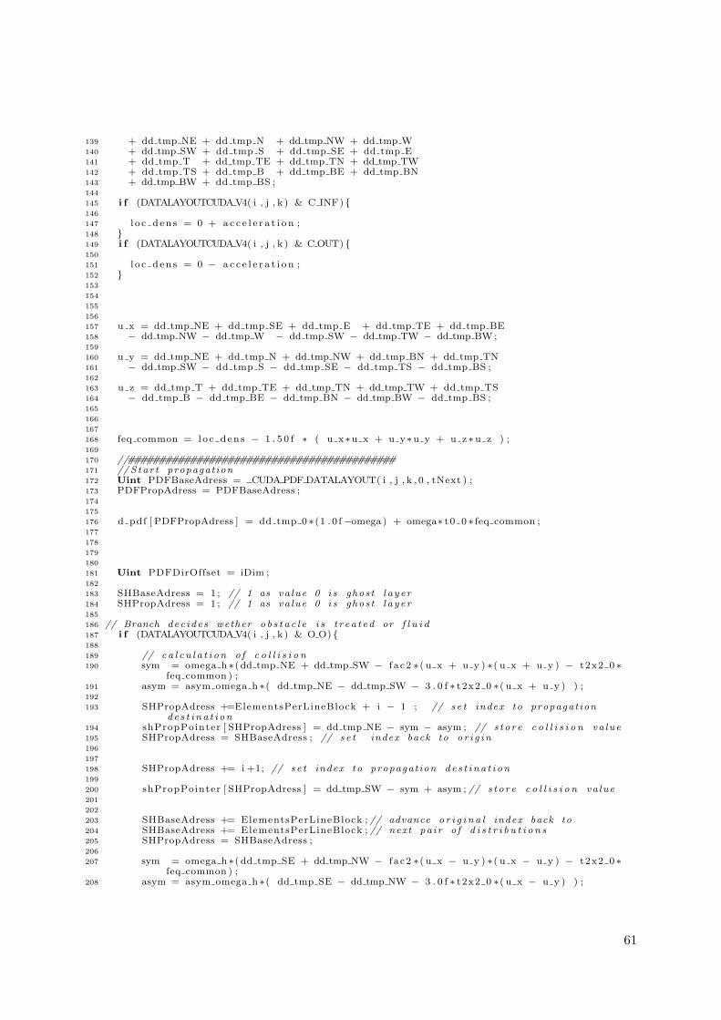
139 + dd tmp NE + dd tmp N + dd tmp NW + dd tmp W140 + dd tmp SW + dd tmp S + dd tmp SE + dd tmp E141 + dd tmp T + dd tmp TE + dd tmp TN + dd tmp TW142 + dd tmp TS + dd tmp B + dd tmp BE + dd tmp BN143 + dd tmp BW + dd tmp BS ;144
145 i f (DATALAYOUTCUDA V4( i , j , k ) & C INF) {146
147 l o c d e n s = 0 + a c c e l e r a t i o n ;148 }149 i f (DATALAYOUTCUDA V4( i , j , k ) & C OUT) {150
151 l o c d e n s = 0 − a c c e l e r a t i o n ;152 }153
154
155
156
157 u x = dd tmp NE + dd tmp SE + dd tmp E + dd tmp TE + dd tmp BE158 − dd tmp NW − dd tmp W − dd tmp SW − dd tmp TW − dd tmp BW ;159
160 u y = dd tmp NE + dd tmp N + dd tmp NW + dd tmp BN + dd tmp TN161 − dd tmp SW − dd tmp S − dd tmp SE − dd tmp TS − dd tmp BS ;162
163 u z = dd tmp T + dd tmp TE + dd tmp TN + dd tmp TW + dd tmp TS164 − dd tmp B − dd tmp BE − dd tmp BN − dd tmp BW − dd tmp BS ;165
166
167
168 feq common = l o c d e n s − 1 . 5 0 f ∗ ( u x∗u x + u y∗u y + u z ∗u z ) ;169
170 //###########################################171 // S ta r t propagat ion172 Uint PDFBaseAdress = CUDA PDF DATALAYOUT( i , j , k , 0 , tNext ) ;173 PDFPropAdress = PDFBaseAdress ;174
175
176 d pdf [ PDFPropAdress ] = dd tmp 0 ∗(1 . 0 f−omega ) + omega∗ t0 0 ∗ feq common ;177
178
179
180
181 Uint PDFDirOffset = iDim ;182
183 SHBaseAdress = 1 ; // 1 as va lue 0 i s ghos t l a y e r184 SHPropAdress = 1 ; // 1 as va lue 0 i s ghos t l a y e r185
186 // Branch dec ides wether o b s t a c l e i s t r e a t ed or f l u i d187 i f (DATALAYOUTCUDA V4( i , j , k ) & O O) {188
189 // c a l c u l a t i o n o f c o l l i s i o n190 sym = omega h ∗( dd tmp NE + dd tmp SW − f a c2 ∗( u x + u y ) ∗( u x + u y ) − t2x2 0 ∗
feq common ) ;191 asym = asym omega h ∗( dd tmp NE − dd tmp SW − 3 . 0 f ∗ t2x2 0 ∗( u x + u y ) ) ;192
193 SHPropAdress +=ElementsPerLineBlock + i − 1 ; // s e t index to propagat ionde s t i na t i on
194 shPropPointer [ SHPropAdress ] = dd tmp NE − sym − asym ; // s t o r e c o l l i s i o n va lue195 SHPropAdress = SHBaseAdress ; // s e t index back to o r i g i n196
197
198 SHPropAdress += i +1; // s e t index to propagat ion de s t i na t i on199
200 shPropPointer [ SHPropAdress ] = dd tmp SW − sym + asym ; // s t o r e c o l l i s i o n va lue201
202
203 SHBaseAdress += ElementsPerLineBlock ; // advance o r i g i n a l index back to204 SHBaseAdress += ElementsPerLineBlock ; // next pa i r o f d i s t r i b u t i o n s205 SHPropAdress = SHBaseAdress ;206
207 sym = omega h ∗( dd tmp SE + dd tmp NW − f a c2 ∗( u x − u y ) ∗( u x − u y ) − t2x2 0 ∗feq common ) ;
208 asym = asym omega h ∗( dd tmp SE − dd tmp NW − 3 . 0 f ∗ t2x2 0 ∗( u x − u y ) ) ;
61
Appendix A Algorithms
209
210 SHPropAdress += ElementsPerLineBlock + i −1;211 shPropPointer [ SHPropAdress ] = dd tmp SE − sym − asym ;212
213 SHPropAdress = SHBaseAdress ;214
215 SHPropAdress += i +1;216 shPropPointer [ SHPropAdress ] = dd tmp NW − sym + asym ;217
218
219 SHBaseAdress += ElementsPerLineBlock ;220 SHBaseAdress += ElementsPerLineBlock ;221 SHPropAdress = SHBaseAdress ;222
223 sym = omega h ∗( dd tmp TE + dd tmp BW − f a c2 ∗( u x + u z ) ∗( u x + u z ) − t2x2 0 ∗feq common ) ;
224 asym = asym omega h ∗( dd tmp TE − dd tmp BW − 3 . 0 f ∗ t2x2 0 ∗( u x + u z ) ) ;225
226 SHPropAdress += ElementsPerLineBlock + i −1;227 shPropPointer [ SHPropAdress ] = dd tmp TE − sym − asym ;228
229 SHPropAdress =SHBaseAdress ;230 SHPropAdress += i +1;231 shPropPointer [ SHPropAdress ] = dd tmp BW − sym + asym ;232
233
234 SHBaseAdress += ElementsPerLineBlock ;235 SHBaseAdress += ElementsPerLineBlock ;236 SHPropAdress = SHBaseAdress ;237
238 sym = omega h ∗( dd tmp BE + dd tmp TW − f a c2 ∗( u x − u z ) ∗( u x − u z ) − t2x2 0 ∗feq common ) ;
239 asym = asym omega h ∗( dd tmp BE − dd tmp TW − 3 . 0 f ∗ t2x2 0 ∗( u x − u z ) ) ;240
241 SHPropAdress += ElementsPerLineBlock +i −1;242 shPropPointer [ SHPropAdress ] = dd tmp BE − sym − asym ;243
244 SHPropAdress =SHBaseAdress ;245 SHPropAdress += i +1;246 shPropPointer [ SHPropAdress ] = dd tmp TW − sym + asym ;247
248 // Treat va lue s not in shared memory249 // advance PDF index to current d i s t r i b u t i o n250 PDFBaseAdress += PDFOffset ; //NE251 PDFBaseAdress += PDFOffset ; //SW252 PDFBaseAdress += PDFOffset ; //SE253 PDFBaseAdress += PDFOffset ; //NW254 PDFBaseAdress += PDFOffset ; //TE255 PDFBaseAdress += PDFOffset ; // BW256 PDFBaseAdress += PDFOffset ; //BE257 PDFBaseAdress += PDFOffset ; //TW258 PDFBaseAdress += PDFOffset ; //TN259 PDFBaseAdress += PDFOffset ; //BS260
261 PDFPropAdress = PDFBaseAdress ;262
263
264 sym = omega h ∗(dd tmp TN + dd tmp BS − f a c2 ∗( u y + u z ) ∗( u y + u z ) − t2x2 0 ∗feq common ) ;
265 asym = asym omega h ∗( dd tmp TN − dd tmp BS − 3 . 0 f ∗ t2x2 0 ∗( u y + u z ) ) ;266
267 PDFPropAdress −= iDim ;268 PDFPropAdress −= iDim∗ jDim ;269 d pdf [ PDFPropAdress ]270 = dd tmp TN − sym − asym ;271
272 PDFBaseAdress −= PDFOffset ; // TN273 PDFPropAdress = PDFBaseAdress ;274
275 PDFPropAdress += iDim∗ jDim ;276 PDFPropAdress += iDim ;277 d pdf [ PDFPropAdress ]278 = dd tmp BS − sym + asym ;
62
279
280 PDFBaseAdress += PDFOffset ; // BS281 PDFBaseAdress += PDFOffset ; //BN282 PDFBaseAdress += PDFOffset ; //TS283 PDFPropAdress = PDFBaseAdress ;284
285 sym = omega h ∗(dd tmp BN + dd tmp TS − f a c2 ∗( u y − u z ) ∗( u y − u z ) − t2x2 0 ∗feq common ) ;
286 asym = asym omega h ∗( dd tmp BN − dd tmp TS − 3 . 0 f ∗ t2x2 0 ∗( u y − u z ) ) ;287
288 PDFPropAdress −= iDim ;289 PDFPropAdress += iDim∗ jDim ;290 d pdf [ PDFPropAdress ]291 = dd tmp BN − sym − asym ;292
293
294 PDFBaseAdress −= PDFOffset ; // BN295 PDFPropAdress = PDFBaseAdress ;296 PDFPropAdress += iDim ;297 PDFPropAdress −= iDim∗ jDim ;298 d pdf [ PDFPropAdress ]299 = dd tmp TS − sym + asym ;300
301
302 PDFBaseAdress += PDFOffset ; //TS303 PDFBaseAdress += PDFOffset ; //N304 PDFBaseAdress += PDFOffset ; //S305 PDFPropAdress = PDFBaseAdress ;306
307 sym = omega h ∗( dd tmp N + dd tmp S − f a c1 ∗u y∗u y − t1x2 0 ∗ feq common ) ;308 asym = asym omega h ∗( dd tmp N − dd tmp S − 3 . 0 f ∗ t1x2 0 ∗u y ) ;309
310 PDFPropAdress −= iDim ;311 d pdf [ PDFPropAdress ] = dd tmp N − sym − asym ;312
313 PDFBaseAdress −= PDFOffset ; // N314 PDFPropAdress = PDFBaseAdress ;315 PDFPropAdress += iDim ;316 d pdf [ PDFPropAdress ]317 = dd tmp S − sym + asym ;318
319 SHBaseAdress += ElementsPerLineBlock ;320 SHBaseAdress += ElementsPerLineBlock ;321 SHPropAdress = SHBaseAdress ;322
323 sym = omega h ∗( dd tmp E + dd tmp W − f a c1 ∗u x∗u x − t1x2 0 ∗ feq common ) ;324 asym = asym omega h ∗( dd tmp E − dd tmp W − 3 . 0 f ∗ t1x2 0 ∗u x ) ;325
326 SHPropAdress +=ElementsPerLineBlock +i −1;327 shPropPointer [ SHPropAdress ] = dd tmp E − sym − asym ;328
329 SHPropAdress = SHBaseAdress ;330 SHPropAdress += i +1;331 shPropPointer [ SHPropAdress ]= dd tmp W − sym + asym ;332
333
334 PDFBaseAdress += PDFOffset ; // S335 PDFBaseAdress += PDFOffset ; // E336 PDFBaseAdress += PDFOffset ; //W337 PDFBaseAdress += PDFOffset ; //T338 PDFBaseAdress += PDFOffset ; // B339 PDFPropAdress = PDFBaseAdress ;340
341 sym = omega h ∗( dd tmp T + dd tmp B − f a c1 ∗u z ∗u z − t1x2 0 ∗ feq common ) ;342 asym = asym omega h ∗( dd tmp T − dd tmp B − 3 . 0 f ∗ t1x2 0 ∗u z ) ;343
344 PDFDirOffset = iDim∗ jDim ;345 PDFPropAdress −= PDFDirOffset ;346
347 d pdf [ PDFPropAdress ]348 = dd tmp T − sym − asym ;349
350 PDFBaseAdress −= PDFOffset ; //T
63
Appendix A Algorithms
351 PDFPropAdress = PDFBaseAdress ;352
353 PDFDirOffset = iDim∗ jDim ;354 PDFPropAdress += PDFDirOffset ;355 d pdf [ PDFPropAdress]= dd tmp B − sym + asym ;356
357 // Treatment o f o b s t a c l e s f i n i s h e d358
359 } else {360 // Treatment o f f l u i d c e l l s361
362 sym = omega h ∗( dd tmp NE + dd tmp SW − f a c2 ∗( u x + u y ) ∗( u x + u y ) − t2x2 0 ∗feq common ) ;
363 asym = asym omega h ∗( dd tmp NE − dd tmp SW − 3 . 0 f ∗ t2x2 0 ∗( u x + u y ) ) ;364
365 SHPropAdress += i +1;366 shPropPointer [ SHPropAdress ] = dd tmp NE − sym − asym ;367 SHPropAdress = SHBaseAdress ;368
369 SHPropAdress += ElementsPerLineBlock + i −1;370 shPropPointer [ SHPropAdress ] = dd tmp SW − sym + asym ;371
372
373 SHBaseAdress += ElementsPerLineBlock ;374 SHBaseAdress += ElementsPerLineBlock ;375 SHPropAdress = SHBaseAdress ;376
377 sym = omega h ∗( dd tmp SE + dd tmp NW − f a c2 ∗( u x − u y ) ∗( u x − u y ) − t2x2 0 ∗feq common ) ;
378 asym = asym omega h ∗( dd tmp SE − dd tmp NW − 3 . 0 f ∗ t2x2 0 ∗( u x − u y ) ) ;379
380 SHPropAdress += i +1;381 shPropPointer [ SHPropAdress ] = dd tmp SE − sym − asym ;382
383 SHPropAdress = SHBaseAdress ;384 SHPropAdress += ElementsPerLineBlock + i −1;385 shPropPointer [ SHPropAdress ] = dd tmp NW − sym + asym ;386
387
388 SHBaseAdress += ElementsPerLineBlock ;389 SHBaseAdress += ElementsPerLineBlock ;390 SHPropAdress = SHBaseAdress ;391
392 sym = omega h ∗( dd tmp TE + dd tmp BW − f a c2 ∗( u x + u z ) ∗( u x + u z ) − t2x2 0 ∗feq common ) ;
393 asym = asym omega h ∗( dd tmp TE − dd tmp BW − 3 . 0 f ∗ t2x2 0 ∗( u x + u z ) ) ;394
395
396 SHPropAdress += i +1;397 shPropPointer [ SHPropAdress ] = dd tmp TE − sym − asym ;398
399 SHPropAdress =SHBaseAdress ;400 SHPropAdress += ElementsPerLineBlock + i −1;401 shPropPointer [ SHPropAdress ] = dd tmp BW − sym + asym ;402
403
404 SHBaseAdress += ElementsPerLineBlock ;405 SHBaseAdress += ElementsPerLineBlock ;406 SHPropAdress = SHBaseAdress ;407
408 sym = omega h ∗( dd tmp BE + dd tmp TW − f a c2 ∗( u x − u z ) ∗( u x − u z ) − t2x2 0 ∗feq common ) ;
409 asym = asym omega h ∗( dd tmp BE − dd tmp TW − 3 . 0 f ∗ t2x2 0 ∗( u x − u z ) ) ;410
411 SHPropAdress += i +1;412 shPropPointer [ SHPropAdress ] = dd tmp BE − sym − asym ;413
414 SHPropAdress =SHBaseAdress ;415 SHPropAdress += ElementsPerLineBlock + i −1;416 shPropPointer [ SHPropAdress ] = dd tmp TW − sym + asym ;417
418
419 PDFBaseAdress += PDFOffset ; //NE
64
420 PDFBaseAdress += PDFOffset ; //SW421 PDFBaseAdress += PDFOffset ; //SE422 PDFBaseAdress += PDFOffset ; //NW423 PDFBaseAdress += PDFOffset ; //TE424 PDFBaseAdress += PDFOffset ; // BW425 PDFBaseAdress += PDFOffset ; //BE426 PDFBaseAdress += PDFOffset ; //TW427 PDFBaseAdress += PDFOffset ; //TN428 PDFPropAdress = PDFBaseAdress ;429
430 sym = omega h ∗(dd tmp TN + dd tmp BS − f a c2 ∗( u y + u z ) ∗( u y + u z ) − t2x2 0 ∗feq common ) ;
431 asym = asym omega h ∗( dd tmp TN − dd tmp BS − 3 . 0 f ∗ t2x2 0 ∗( u y + u z ) ) ;432
433 // Macro tha t implements p e r i od i c boundary cond i t i on fo r t e s t c a s e s434 #ifdef PERIODICY435 i f ( j > jDim−3){436 PDFPropAdress −= iDim ∗( jDim−3) ;437 } else {438 #else i f439 {440 #endif441 PDFPropAdress += iDim ;442 }443
444 PDFPropAdress += iDim∗ jDim ;445 d pdf [ PDFPropAdress ]446 = dd tmp TN − sym − asym ;447
448 PDFBaseAdress += PDFOffset ;449 PDFPropAdress = PDFBaseAdress ;450 PDFPropAdress −= iDim∗ jDim ;451
452 // Macro tha t implements p e r i od i c boundary cond i t i on fo r t e s t c a s e s453 #ifdef PERIODICY454 i f ( j < 2) {455 PDFPropAdress += iDim ∗( jDim−3) ;456 } else {457 #else i f458 {459 #endif460 PDFPropAdress −= iDim ;461 }462
463 d pdf [ PDFPropAdress ]464 = dd tmp BS − sym + asym ;465
466
467
468 PDFBaseAdress += PDFOffset ;469 PDFPropAdress = PDFBaseAdress ;470
471 sym = omega h ∗(dd tmp BN + dd tmp TS − f a c2 ∗( u y − u z ) ∗( u y − u z ) − t2x2 0 ∗feq common ) ;
472 asym = asym omega h ∗( dd tmp BN − dd tmp TS − 3 . 0 f ∗ t2x2 0 ∗( u y − u z ) ) ;473
474 // Macro tha t implements p e r i od i c boundary cond i t i on fo r t e s t c a s e s475 #ifdef PERIODICY476 i f ( j > jDim−3){477
478 PDFPropAdress −= iDim ∗( jDim−3) ;479 } else {480 #else i f481 {482 #endif483 PDFPropAdress += iDim ;484 }485
486 PDFPropAdress −= iDim∗ jDim ;487 d pdf [ PDFPropAdress ]488 = dd tmp BN − sym − asym ;489
490
65
Appendix A Algorithms
491 PDFBaseAdress += PDFOffset ;492 PDFPropAdress = PDFBaseAdress ;493
494 // Macro tha t implements p e r i od i c boundary cond i t i on fo r t e s t c a s e s495 #ifdef PERIODICY496 i f ( j < 2) {497 PDFPropAdress += iDim ∗( jDim−3) ;498 } else {499 #else i f500 {501 #endif502 PDFPropAdress −= iDim ;503 }504
505 PDFPropAdress += iDim∗ jDim ;506 d pdf [ PDFPropAdress ]507 = dd tmp TS − sym + asym ;508
509
510 PDFBaseAdress += PDFOffset ;511 PDFPropAdress = PDFBaseAdress ;512
513 sym = omega h ∗( dd tmp N + dd tmp S − f a c1 ∗u y∗u y − t1x2 0 ∗ feq common ) ;514 asym = asym omega h ∗( dd tmp N − dd tmp S − 3 . 0 f ∗ t1x2 0 ∗u y ) ;515
516 // Macro tha t implements p e r i od i c boundary cond i t i on fo r t e s t c a s e s517 #ifdef PERIODICY518 i f ( j > jDim−3){519 PDFPropAdress −= iDim ∗( jDim−3) ;520 } else {521 #else i f522 {523 #endif524 PDFPropAdress += iDim ;525 }526 d pdf [ PDFPropAdress ]527 = dd tmp N − sym − asym ;528
529 PDFBaseAdress += PDFOffset ;530 PDFPropAdress = PDFBaseAdress ;531
532 // Macro tha t implements p e r i od i c boundary cond i t i on fo r t e s t c a s e s533 #ifdef PERIODICY534 i f ( j < 2) {535 PDFPropAdress += iDim ∗( jDim−3) ;536 } else {537 #else i f538 {539 #endif540 PDFPropAdress −= iDim ;541 }542
543
544 d pdf [ PDFPropAdress ] ‘545 = dd tmp S − sym + asym ;546
547 SHBaseAdress += ElementsPerLineBlock ;548 SHBaseAdress += ElementsPerLineBlock ;549 SHPropAdress = SHBaseAdress ;550
551 sym = omega h ∗( dd tmp E + dd tmp W − f a c1 ∗u x∗u x − t1x2 0 ∗ feq common ) ;552 asym = asym omega h ∗( dd tmp E − dd tmp W − 3 . 0 f ∗ t1x2 0 ∗u x ) ;553
554 SHPropAdress += i +1;555 shPropPointer [ SHPropAdress ] = dd tmp E − sym − asym ;556
557 SHPropAdress = SHBaseAdress ;558 SHPropAdress += ElementsPerLineBlock +i −1;559 shPropPointer [ SHPropAdress ]= dd tmp W − sym + asym ;560
561
562 PDFBaseAdress += PDFOffset ; // E563 PDFBaseAdress += PDFOffset ; // W
66
564 PDFBaseAdress += PDFOffset ; // T565 PDFPropAdress = PDFBaseAdress ;566
567 sym = omega h ∗( dd tmp T + dd tmp B − f a c1 ∗u z ∗u z − t1x2 0 ∗ feq common ) ;568 asym = asym omega h ∗( dd tmp T − dd tmp B − 3 . 0 f ∗ t1x2 0 ∗u z ) ;569
570 PDFDirOffset = iDim∗ jDim ;571 PDFPropAdress += PDFDirOffset ;572 d pdf [ PDFPropAdress ]573 = dd tmp T − sym − asym ;574
575 PDFBaseAdress += PDFOffset ; //B576 PDFPropAdress = PDFBaseAdress ;577 PDFDirOffset = iDim∗ jDim ;578 PDFPropAdress −= PDFDirOffset ;579 d pdf [ PDFPropAdress]=580 dd tmp B − sym + asym ;581
582
583
584
585
586 }587
588
589
590
591
592 // Write bu f f e r e d propagat ions from shared memory to g l o b a l memory593
594 sync th r ead s ( ) ; // synchronize shared memory wr i t e s595
596 // Set i nde c i e s to o r i g i n s597 SHBaseAdress = 1 ;598 SHPropAdress =SHBaseAdress ;599 PDFOffset = ( iDim∗ jDim∗kDim) ;600 PDFBaseAdress += PDFOffset ;601 PDFPropAdress = PDFBaseAdress ;602
603 // Macro tha t implements p e r i od i c boundary cond i t i on fo r t e s t c a s e s604 #ifdef PERIODICY605 i f ( j > jDim−3){606
607 PDFDirOffset = iDim ∗( jDim−3) ;608 PDFPropAdress −= PDFDirOffset ;609
610 } else {611 #else i f612 {613 #endif614 PDFDirOffset = iDim ;615 PDFPropAdress += PDFDirOffset ;616 }617
618 SHPropAdress += i ;619 d pdf [ PDFPropAdress]= shPropPointer [ SHPropAdress ] ;620
621 SHPropAdress = SHBaseAdress ;622 PDFBaseAdress += PDFOffset ;623 PDFPropAdress = PDFBaseAdress ;624
625 // Macro tha t implements p e r i od i c boundary cond i t i on fo r t e s t c a s e s626 #ifdef PERIODICY627 i f ( j < 2) {628
629 PDFDirOffset = iDim ∗( jDim−3) ;630 PDFPropAdress += PDFDirOffset ;631
632 } else {633 #else i f634 {635 #endif636 PDFDirOffset = iDim ;
67
Appendix A Algorithms
637 PDFPropAdress −= PDFDirOffset ;638 }639
640 SHPropAdress += ElementsPerLineBlock + i ;641 d pdf [ PDFPropAdress ]642 = shPropPointer [ SHPropAdress ] ;643
644 SHBaseAdress += ElementsPerLineBlock ;645 SHBaseAdress += ElementsPerLineBlock ;646 SHPropAdress = SHBaseAdress ;647
648
649 PDFBaseAdress += PDFOffset ;650 PDFPropAdress = PDFBaseAdress ;651
652 // Macro tha t implements p e r i od i c boundary cond i t i on fo r t e s t c a s e s653 #ifdef PERIODICY654 i f ( j < 2) {655
656 PDFDirOffset = iDim ∗( jDim−3) ;657 PDFPropAdress += PDFDirOffset ;658
659 } else {660 #else i f661 {662 #endif663 PDFDirOffset = iDim ;664 PDFPropAdress −= PDFDirOffset ;665 }666 SHPropAdress += i ;667 d pdf [ PDFPropAdress ]668 = shPropPointer [ SHPropAdress ] ;669
670
671
672 SHPropAdress = SHBaseAdress ;673 PDFBaseAdress += PDFOffset ;674 PDFPropAdress = PDFBaseAdress ;675
676 // Macro tha t implements p e r i od i c boundary cond i t i on fo r t e s t c a s e s677 #ifdef PERIODICY678 i f ( j > jDim−3){679
680 PDFDirOffset = iDim ∗( jDim−3) ;681 PDFPropAdress −= PDFDirOffset ;682
683 } else {684 #else i f685 {686 #endif687 PDFDirOffset = iDim ;688 PDFPropAdress += PDFDirOffset ;689 }690
691 SHPropAdress += ElementsPerLineBlock + i ;692 d pdf [ PDFPropAdress ]693 = shPropPointer [ SHPropAdress ] ;694
695
696 SHBaseAdress += ElementsPerLineBlock ;697 SHBaseAdress += ElementsPerLineBlock ;698 SHPropAdress =SHBaseAdress ;699
700 PDFBaseAdress += PDFOffset ;701 PDFPropAdress = PDFBaseAdress ;702
703 PDFDirOffset = iDim∗ jDim ;704 PDFPropAdress += PDFDirOffset ;705
706
707 SHPropAdress += i ;708 d pdf [ PDFPropAdress ]709 = shPropPointer [ SHPropAdress ] ;
68
710
711 SHPropAdress = SHBaseAdress ;712 PDFBaseAdress += PDFOffset ;713 PDFPropAdress = PDFBaseAdress ;714
715 PDFDirOffset = iDim∗ jDim ;716 PDFPropAdress −= PDFDirOffset ;717
718 SHPropAdress += ElementsPerLineBlock + i ;719 d pdf [ PDFPropAdress ]720 = shPropPointer [ SHPropAdress ] ;721
722 SHBaseAdress += ElementsPerLineBlock ;723 SHBaseAdress += ElementsPerLineBlock ;724 SHPropAdress = SHBaseAdress ;725
726
727 PDFBaseAdress += PDFOffset ;728 PDFPropAdress = PDFBaseAdress ;729
730 PDFDirOffset = iDim∗ jDim ;731 PDFPropAdress −= PDFDirOffset ;732
733 SHPropAdress += i ;734
735 d pdf [ PDFPropAdress ]736 = shPropPointer [ SHPropAdress ] ;737
738 SHPropAdress = SHBaseAdress ;739 PDFBaseAdress += PDFOffset ;740 PDFPropAdress = PDFBaseAdress ;741 PDFDirOffset = iDim∗ jDim ;742 PDFPropAdress += PDFDirOffset ;743
744
745 SHPropAdress += ElementsPerLineBlock + i ;746 d pdf [ PDFPropAdress ]747 = shPropPointer [ SHPropAdress ] ;748
749 SHBaseAdress += ElementsPerLineBlock ;750 SHBaseAdress += ElementsPerLineBlock ;751 SHPropAdress =SHBaseAdress ;752
753
754 PDFBaseAdress += PDFOffset ;755 PDFBaseAdress += PDFOffset ;756 PDFBaseAdress += PDFOffset ;757 PDFBaseAdress += PDFOffset ;758 PDFBaseAdress += PDFOffset ;759 PDFBaseAdress += PDFOffset ;760 PDFBaseAdress += PDFOffset ;761 PDFPropAdress = PDFBaseAdress ;762
763 SHPropAdress += i ;764 d pdf [ PDFPropAdress ]765 = shPropPointer [ SHPropAdress ] ;766
767
768 SHPropAdress = SHBaseAdress ;769 PDFBaseAdress += PDFOffset ;770 PDFPropAdress = PDFBaseAdress ;771 SHPropAdress += ElementsPerLineBlock + i ;772 d pdf [ PDFPropAdress ]773 = shPropPointer [ SHPropAdress ] ;774
775
776 sync th r ead s ( ) ;777
778
779 }
69

Appendix A Algorithms
´
70
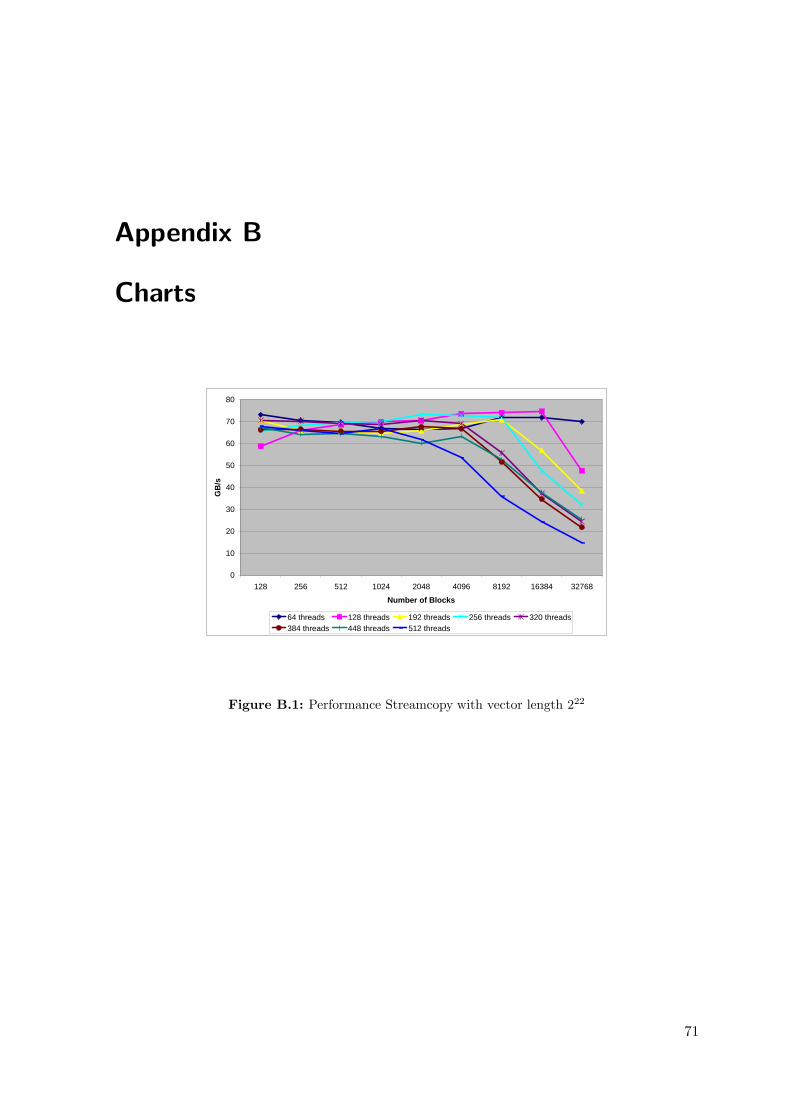
Appendix B
Charts
0
10
20
30
40
50
60
70
80
128 256 512 1024 2048 4096 8192 16384 32768
Number of Blocks
GB
/s
64 threads 128 threads 192 threads 256 threads 320 threads384 threads 448 threads 512 threads
Figure B.1: Performance Streamcopy with vector length 222
71
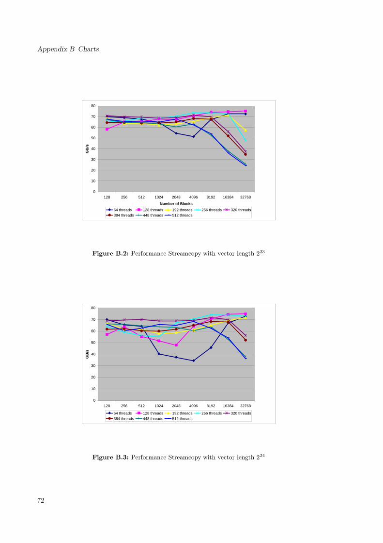
Appendix B Charts
0
10
20
30
40
50
60
70
80
128 256 512 1024 2048 4096 8192 16384 32768
Number of Blocks
GB
/s
64 threads 128 threads 192 threads 256 threads 320 threads384 threads 448 threads 512 threads
Figure B.2: Performance Streamcopy with vector length 223
0
10
20
30
40
50
60
70
80
128 256 512 1024 2048 4096 8192 16384 32768
Number of Blocks
GB
/s
64 threads 128 threads 192 threads 256 threads 320 threads384 threads 448 threads 512 threads
Figure B.3: Performance Streamcopy with vector length 224
72
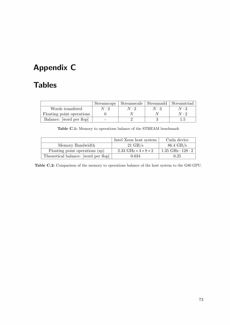
Appendix C
Tables
Streamcopy Streamscale Streamadd StreamtriadWords transfered N · 2 N · 2 N · 3 N · 3
Floating point operations 0 N N N · 2Balance: [word per flop] - 2 3 1.5
Table C.1: Memory to operations balance of the STREAM benchmark
Intel Xeon host system Cuda deviceMemory Bandwidth 21 GB/s 86.4 GB/s
Floating point operations (sp) 2.33 GHz ∗ 4 ∗ 8 ∗ 2 1.35 GHz · 128 · 2Theoretical balance: [word per flop] 0.034 0.25
Table C.2: Comparison of the memory to operations balance of the host system to the G80 GPU.
73

Appendix C Tables
74
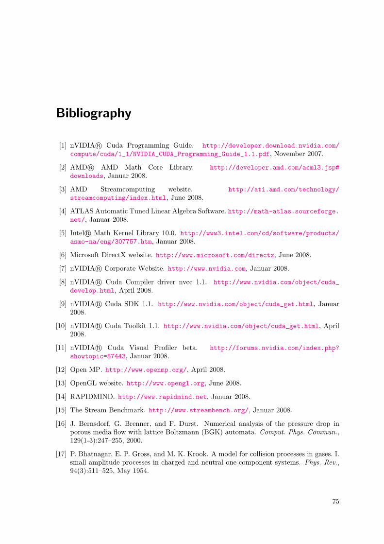
Bibliography
[1] nVIDIA R© Cuda Programming Guide. http://developer.download.nvidia.com/compute/cuda/1_1/NVIDIA_CUDA_Programming_Guide_1.1.pdf, November 2007.
[2] AMD R© AMD Math Core Library. http://developer.amd.com/acml3.jsp#downloads, Januar 2008.
[3] AMD Streamcomputing website. http://ati.amd.com/technology/streamcomputing/index.html, June 2008.
[4] ATLAS Automatic Tuned Linear Algebra Software. http://math-atlas.sourceforge.net/, Januar 2008.
[5] Intel R© Math Kernel Library 10.0. http://www3.intel.com/cd/software/products/asmo-na/eng/307757.htm, Januar 2008.
[6] Microsoft DirectX website. http://www.microsoft.com/directx, June 2008.
[7] nVIDIA R© Corporate Website. http://www.nvidia.com, Januar 2008.
[8] nVIDIA R© Cuda Compiler driver nvcc 1.1. http://www.nvidia.com/object/cuda_develop.html, April 2008.
[9] nVIDIA R© Cuda SDK 1.1. http://www.nvidia.com/object/cuda_get.html, Januar2008.
[10] nVIDIA R© Cuda Toolkit 1.1. http://www.nvidia.com/object/cuda_get.html, April2008.
[11] nVIDIA R© Cuda Visual Profiler beta. http://forums.nvidia.com/index.php?showtopic=57443, Januar 2008.
[12] Open MP. http://www.openmp.org/, April 2008.
[13] OpenGL website. http://www.opengl.org, June 2008.
[14] RAPIDMIND. http://www.rapidmind.net, Januar 2008.
[15] The Stream Benchmark. http://www.streambench.org/, Januar 2008.
[16] J. Bernsdorf, G. Brenner, and F. Durst. Numerical analysis of the pressure drop inporous media flow with lattice Boltzmann (BGK) automata. Comput. Phys. Commun.,129(1-3):247–255, 2000.
[17] P. Bhatnagar, E. P. Gross, and M. K. Krook. A model for collision processes in gases. I.small amplitude processes in charged and neutral one-component systems. Phys. Rev.,94(3):511–525, May 1954.
75
Bibliography
[18] F. Durst. Grundlagen der Stromungsmechanik: Eine Einfuhrung in die Theorie derStromung von Fluiden. Springer, Berlin, 2006.
[19] D. Goddeke, R. Strzodka, J. Mohd-Yusof, P. McCormick, S. H. Buijssen, M. Grajewski,and S. Turek. Exploring weak scalability for FEM calculations on a GPU-enhancedcluster. Parallel Computing, 33(10–11):685–699, 2007.
[20] D. Goddeke, R. Strzodka, and S. Turek. Performance and accuracy of hardware-orientednative-, emulated- and mixed-precision solvers in FEM simulations. International Jour-nal of Parallel, Emergent and Distributed Systems, 22(4):221–256, Aug. 2007.
[21] J. Habich. Improving computational efficiency of lattice Boltzmann methods on com-plex geometries. Bachelor’s thesis, Chair of System Simulation, University of Erlangen-Nuremberg, Germany, 2006.
[22] G. Hager, T. Zeiser, and G. Wellein. Data access optimizations for highly threadedmulti-core CPUs with multiple memory controllers. In Workshop on Large-Scale ParallelProcessing 2008 (IPDPS2008), Miami, FL, April 18, 2008.
[23] K. Iglberger. Performance Analysis and Optimization of the Lattice Boltzmann Methodin 3D. Bachelor’s thesis, Chair of System Simulation, University of Erlangen-Nuremberg,Germany, 2003.
[24] A. J. C. Ladd. Numerical simulations of particulate suspensions via a discrete Boltzmannequation. part 1. theoretical foundation. J. Fluid Mech., 271:285–309, 1994.
[25] A. J. C. Ladd. Numerical simulations of particulate suspensions via a discrete Boltzmannequation. part 2. numerical results. J. Fluid Mech., 271:311–339, 1994.
[26] W. Lie, X. Wei, and Arie Kaufmann. Implementing Lattice Boltzmann Computation onGraphics Hardware. The Visual Computer, 19(7-8):444–456, 2003.
[27] J. Michalakes and M. Vachharajani. GPU acceleration of numerical weather prediction.In Workshop on Large Scale Parallel Processing 2008 (IPDPS2008), Miami, FL, April18, 2008.
[28] O. Pickenacker. Gestufte Verbrennung in porosen Medien. PhD thesis, UniversityErlangen-Nuremberg, 2001.
[29] A. Prosperetti and G. Tryggvason. Computational Methods for Multiphase Flow. Cam-bridge University Press, Cambridge, 2007.
[30] Y. H. Qian, D. d’Humieres, and P. Lallemand. Lattice BGK models for Navier-Stokesequation. Europhys. Lett., 17(6):479–484, Jan. 1992.
[31] J. Tolke and M. Krafczyk. Towards three-dimensional teraflop CFD computing on adesktop pc using graphics hardware. In Proceedings of International Conference forMesoscopic Methods in Engineering and Science ICMMES07, Munich, 2007.
[32] G. Wellein, T. Zeiser, G. Hager, and S. Donath. On the single processor performance ofsimple lattice Boltzmann kernels. Computers & Fluids, 35:910–919, 2006.
76
Erklarung:
Ich versichere, dass ich die Arbeit ohne fremde Hilfe und ohne Benutzung anderer als derangegebenen Quellen angefertigt habe und dass die Arbeit in gleicher oder ahnlicher Formnoch keiner anderen Prufungsbehorde vorgelegen hat und von dieser als Teil einer Prufungsleis-tung angenommen wurde. Alle Ausfuhrungen, die wortlich oder sinngemaß ubernommenwurden, sind als solche gekennzeichnet.
Erlangen, den 01.07.2008 . . . . . . . . . . . . . . . . . . . . . . . . . . . . . . . .