Physics C

Chapter 18

Superposition and Standing Waves

Dr. khitam Y. Elwasife

Waves vs. Particles

Waves are very different from particles.

Particles have zero size. Waves have a characteristic size – their

wavelength.

Multiple particles must exist at

different locations.

Multiple waves can combine at one point in

the same medium – they can be present at

the same location.

Introduction

Chapter 18, Superposition and Standing Waves

Superposition

Interference

Standing Waves Nodes, Anti-nodes

Quantization

When waves are combined in systems with boundary conditions, only certain allowed frequencies can exist.

We say the frequencies are quantized.

Quantization is at the heart of quantum mechanics.

The analysis of waves under boundary conditions explains many quantum phenomena.

Quantization can be used to understand the behavior of the wide array of musical instruments that are based on strings and air columns.

Waves can also combine when they have different frequencies.

Introduction

Superposition Principle

Waves can be combined in the same location in space.

To analyze these wave combinations, use the superposition principle:

If two or more traveling waves are moving through a medium, the resultant value of the wave function at any point is the algebraic sum of the values of the wave functions of the individual waves.

Waves that obey the superposition principle are linear waves.

For mechanical waves, linear waves have amplitudes much smaller than

their wavelengths.

Section 18.1

Superposition and Interference

Two traveling waves can pass through each other without being destroyed or

altered.

A consequence of the superposition principle.

The combination of separate waves in the same region of space to produce a

resultant wave is called interference.

The term interference has a very specific usage in physics.

It means waves pass through each other.

Section 18.1

Superposition Example

Two pulses are traveling in opposite

directions (a).

The wave function of the pulse

moving to the right is y1 and for the

one moving to the left is y2.

The pulses have the same speed but

different shapes.

The displacement of the elements is

positive for both.

When the waves start to overlap (b),

the resultant wave function is y1 + y2.

Section 18.1

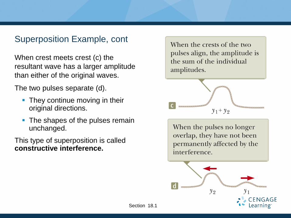
Superposition Example, cont

When crest meets crest (c) the

resultant wave has a larger amplitude

than either of the original waves.

The two pulses separate (d).

They continue moving in their original directions.

The shapes of the pulses remain unchanged.

This type of superposition is called constructive interference.

Section 18.1

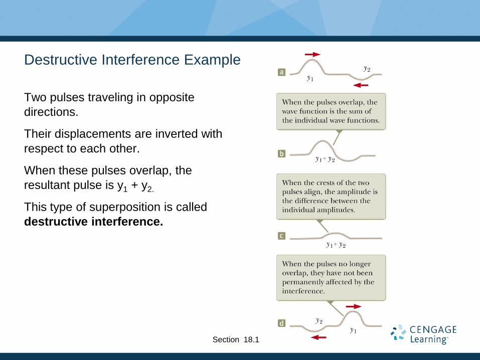
Destructive Interference Example

Two pulses traveling in opposite

directions.

Their displacements are inverted with

respect to each other.

When these pulses overlap, the

resultant pulse is y1 + y2.

This type of superposition is called

destructive interference.

Section 18.1

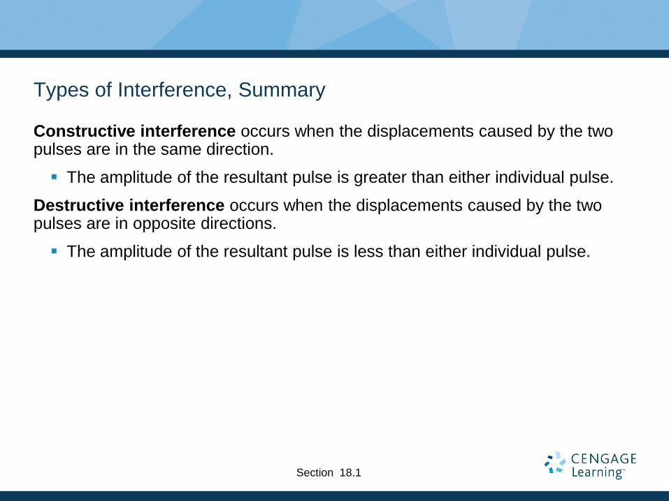
Types of Interference, Summary

Constructive interference occurs when the displacements caused by the two pulses are in the same direction.

The amplitude of the resultant pulse is greater than either individual pulse.

Destructive interference occurs when the displacements caused by the two pulses are in opposite directions.

The amplitude of the resultant pulse is less than either individual pulse.

Section 18.1

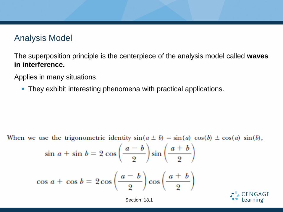
Analysis Model

The superposition principle is the centerpiece of the analysis model called waves

in interference.

Applies in many situations

They exhibit interesting phenomena with practical applications.

Section 18.1

Superposition of Sinusoidal Waves

Assume two waves are traveling in the same direction in a linear medium, with the same frequency, wavelength and amplitude.

The waves differ only in phase:

y1 = A sin (kx - wt)

y2 = A sin (kx - wt + f)

y = y1+y2 = 2A cos (f /2) sin (kx - wt + f /2)

The resultant wave function, y, is also sinusoida.l

The resultant wave has the same frequency and wavelength as the original waves.

The amplitude of the resultant wave is 2A cos (f / 2) .

The phase of the resultant wave is f / 2.

Sinusoidal Waves with Constructive Interference

When f = 0, then cos (f/2) = 1

The amplitude of the resultant wave is 2A.

The crests of the two waves are at the same location in space.

The waves are everywhere in phase.

The waves interfere constructively.

In general, constructive interference occurs when cos (Φ/2) = ± 1.

That is, when Φ = 0, 2π, 4π, … rad

When Φ is an even multiple of π

Section 18.1

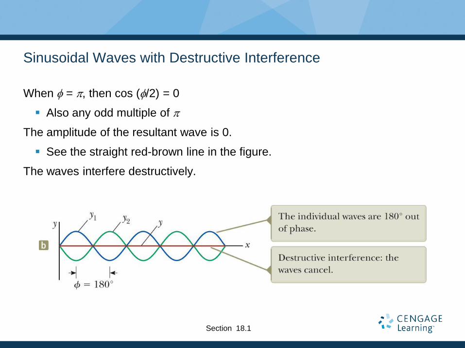
Sinusoidal Waves with Destructive Interference

When f = p, then cos (f/2) = 0

Also any odd multiple of p

The amplitude of the resultant wave is 0.

See the straight red-brown line in the figure.

The waves interfere destructively.

Section 18.1

Sinusoidal Waves, General Interference

When f is other than 0 or an even multiple of p, the amplitude of the resultant is between 0 and 2A.

The wave functions still add

The interference is neither constructive nor destructive.

Section 18.1

Sinusoidal Waves, Summary of Interference

Constructive interference occurs when f = np where n is an even integer

(including 0).

Amplitude of the resultant is 2A

Destructive interference occurs when f = np where n is an odd integer.

Amplitude is 0

General interference occurs when 0 < f < np

Amplitude is 0 < Aresultant < 2A

Section 18.1

Sinusoidal Waves, Interference with Difference Amplitudes

Constructive interference occurs when f = n p where n is an even integer

(including 0).

Amplitude of the resultant is the sum of the amplitudes of the waves

Destructive interference occurs when f = n p where n is an odd integer.

Amplitude is less, but the amplitudes do not completely cancel

Section 18.1

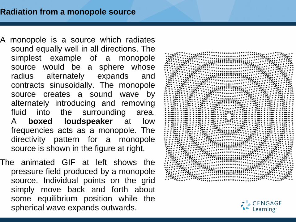
Radiation from a monopole source

A monopole is a source which radiates sound equally well in all directions. The simplest example of a monopole source would be a sphere whose radius alternately expands and contracts sinusoidally. The monopole source creates a sound wave by alternately introducing and removing fluid into the surrounding area. A boxed loudspeaker at low frequencies acts as a monopole. The directivity pattern for a monopole source is shown in the figure at right.

The animated GIF at left shows the pressure field produced by a monopole source. Individual points on the grid simply move back and forth about some equilibrium position while the spherical wave expands outwards.

Radiation from a dipole source

A dipole source consists of two monopole

sources of equal strength but opposite

phase and separated by a small distance

compared with the wavelength of sound.

While one source expands the other source

contracts. The result is that the fluid (air)

near the two sources sloshes back and

forth to produce the sound. A sphere which

oscillates back and forth acts like a dipole

source, as does an unboxed loudspeaker .

A dipole source does not radiate sound in

all directions equally. The directivity pattern

shown at right looks like a figure-8; there

are two regions where sound is radiated

very well, and two regions where sound

cancels. the wavefronts expanding to the

right and left are 180o out of phase with

each other.

.

Radiation from a lateral quadrupole source

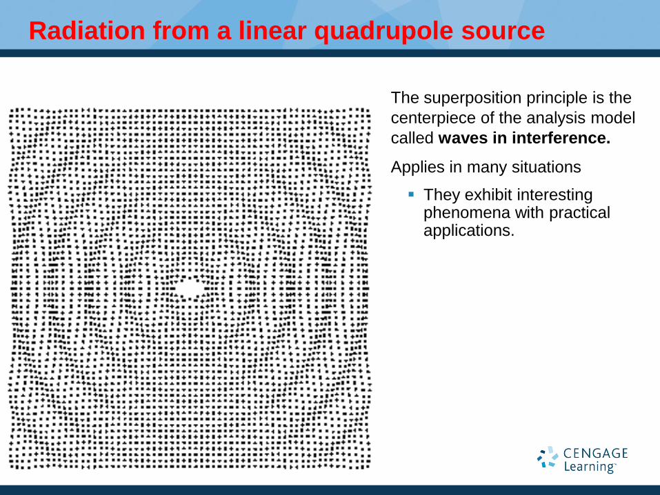
Radiation from a linear quadrupole source

The superposition principle is the

centerpiece of the analysis model

called waves in interference.

Applies in many situations

They exhibit interesting phenomena with practical applications.

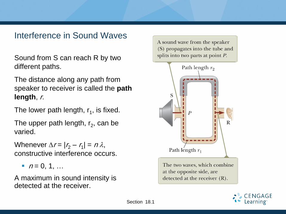
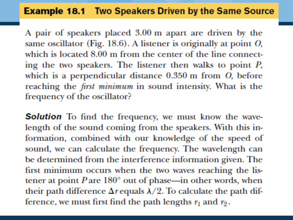
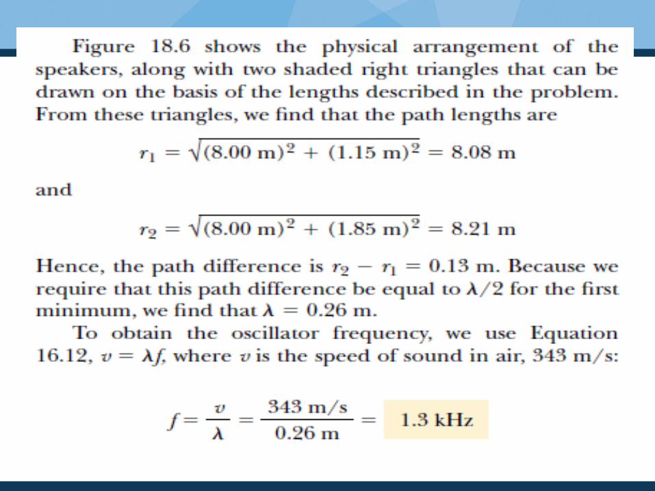
Interference in Sound Waves

Sound from S can reach R by two

different paths.

The distance along any path from

speaker to receiver is called the path

length, r.

The lower path length, r1, is fixed.

The upper path length, r2, can be

varied.

Whenever Dr = |r2 – r1| = n l,

constructive interference occurs.

n = 0, 1, …

A maximum in sound intensity is detected at the receiver.

Section 18.1

Interference in Sound Waves, 2

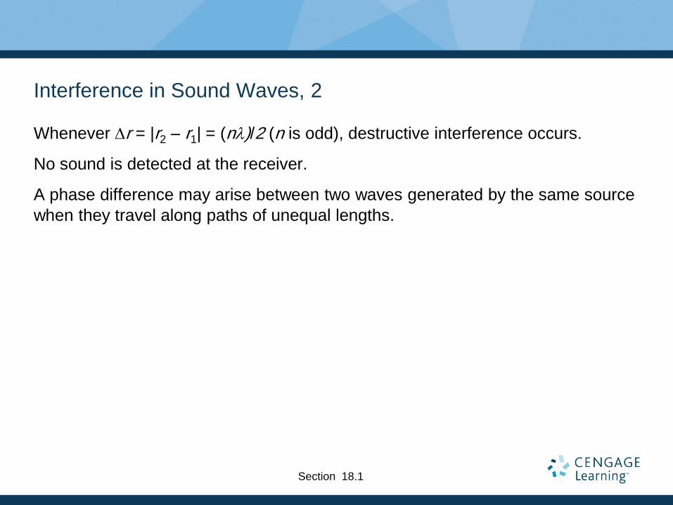
Whenever Dr = |r2 – r1| = (nl)/2 (n is odd), destructive interference occurs.

No sound is detected at the receiver.

A phase difference may arise between two waves generated by the same source

when they travel along paths of unequal lengths.

Section 18.1

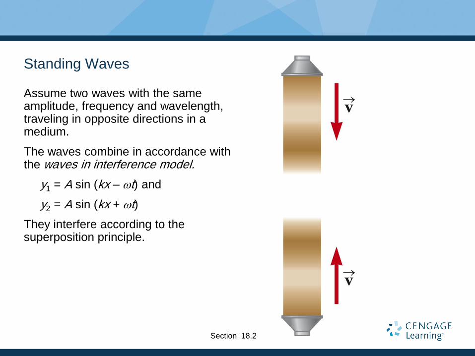
Standing Waves

Assume two waves with the same amplitude, frequency and wavelength, traveling in opposite directions in a medium.

The waves combine in accordance with the waves in interference model.

y1 = A sin (kx – wt) and

y2 = A sin (kx + wt)

They interfere according to the superposition principle.

Section 18.2

Standing Waves, cont

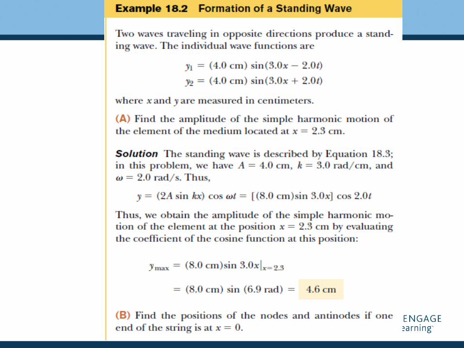
The resultant wave will be y = (2A sin kx) cos wt.

This is the wave function of a standing wave.

There is no kx – wt term, and therefore it is not a traveling wave.

In observing a standing wave, there is no sense of motion in the direction of propagation of either of the original waves.

Section 18.2

Standing Wave Example

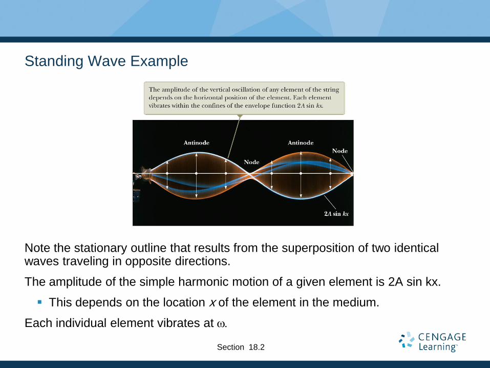
Note the stationary outline that results from the superposition of two identical waves traveling in opposite directions.

The amplitude of the simple harmonic motion of a given element is 2A sin kx.

This depends on the location x of the element in the medium.

Each individual element vibrates at w

Section 18.2

Note on Amplitudes

There are three types of amplitudes used in describing waves.

The amplitude of the individual waves, A

The amplitude of the simple harmonic motion of the elements in the medium,

2A sin kx

A given element in the standing wave vibrates within the constraints of the

envelope function 2 A sin k x.

The amplitude of the standing wave, 2A

Section 18.2

Standing Waves, Definitions

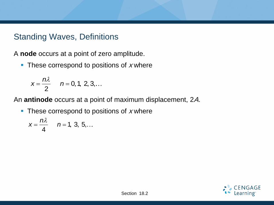
A node occurs at a point of zero amplitude.

These correspond to positions of x where

An antinode occurs at a point of maximum displacement, 2A.

These correspond to positions of x where

0,1, 2, 3,2

nx n

l

1, 3, 5,4

nx n

l

Section 18.2

Features of Nodes and Antinodes

The distance between adjacent antinodes is l/2.

The distance between adjacent nodes is l/2.

The distance between a node and an adjacent antinode is l/4.

Section 18.2

Nodes and Antinodes, cont

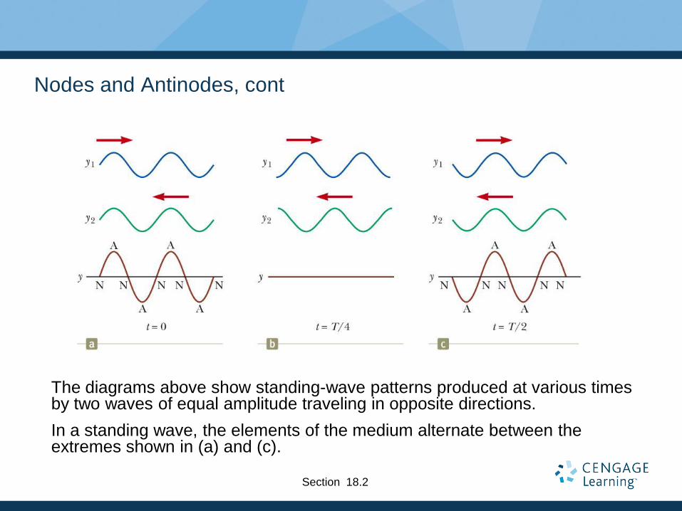
The diagrams above show standing-wave patterns produced at various times by two waves of equal amplitude traveling in opposite directions.

In a standing wave, the elements of the medium alternate between the extremes shown in (a) and (c).

Section 18.2

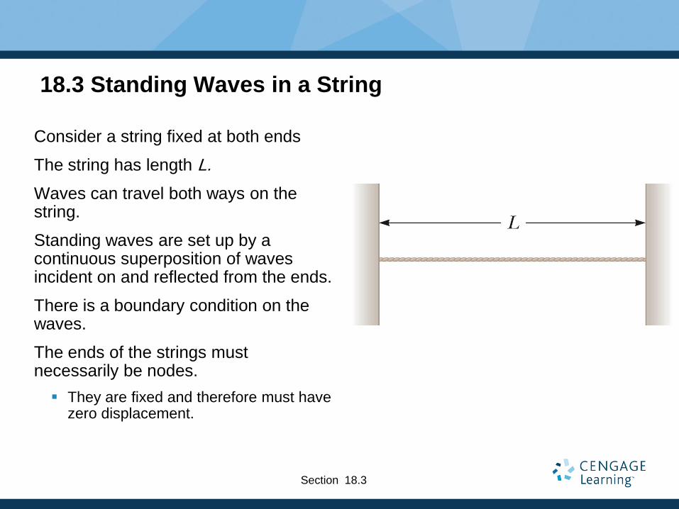
18.3 Standing Waves in a String

Consider a string fixed at both ends

The string has length L.

Waves can travel both ways on the string.

Standing waves are set up by a continuous superposition of waves incident on and reflected from the ends.

There is a boundary condition on the waves.

The ends of the strings must necessarily be nodes.

They are fixed and therefore must have zero displacement.

Section 18.3

The boundary condition results in the string having a set of natural patterns of oscillation, called normal modes.

Each mode has a characteristic frequency.

This situation in which only certain frequencies of oscillations are allowed is called quantization.

The normal modes of oscillation for the string can be described by imposing the requirements that the ends be nodes and that the nodes and antinodes are separated by λ/4.

We identify an analysis model called waves under boundary conditions.

Section 18.3

This is the first normal mode that is consistent with the boundary conditions.

There are nodes at both ends.

There is one antinode in the middle.

This is the longest wavelength mode:

½l1 = L so l1 = 2L

The section of the standing wave between nodes is called a loop.

In the first normal mode, the string vibrates in one loop.

Section 18.3

Consecutive normal modes add a loop at each step.

The section of the standing wave from one node to the next is called a loop.

The second mode (c) corresponds to to l = L.

The third mode (d) corresponds to l = 2L/3. Section 18.3

Standing Waves on a String, Summary

The wavelengths of the normal modes for a string of length L fixed at both ends are ln = 2L / n n = 1, 2, 3, …

n is the nth normal mode of oscillation

These are the possible modes for the string:

The natural frequencies are

Also called quantized frequencies

ƒ2 2

n

v n Tn

L L

Section 18.3

Waves on a String, Harmonic Series

The fundamental frequency corresponds to n = 1.

It is the lowest frequency, ƒ1

The frequencies of the remaining natural modes are integer multiples of the fundamental frequency.

ƒn = nƒ1

Frequencies of normal modes that exhibit this relationship form a harmonic series.

The normal modes are called harmonics.

Section 18.3

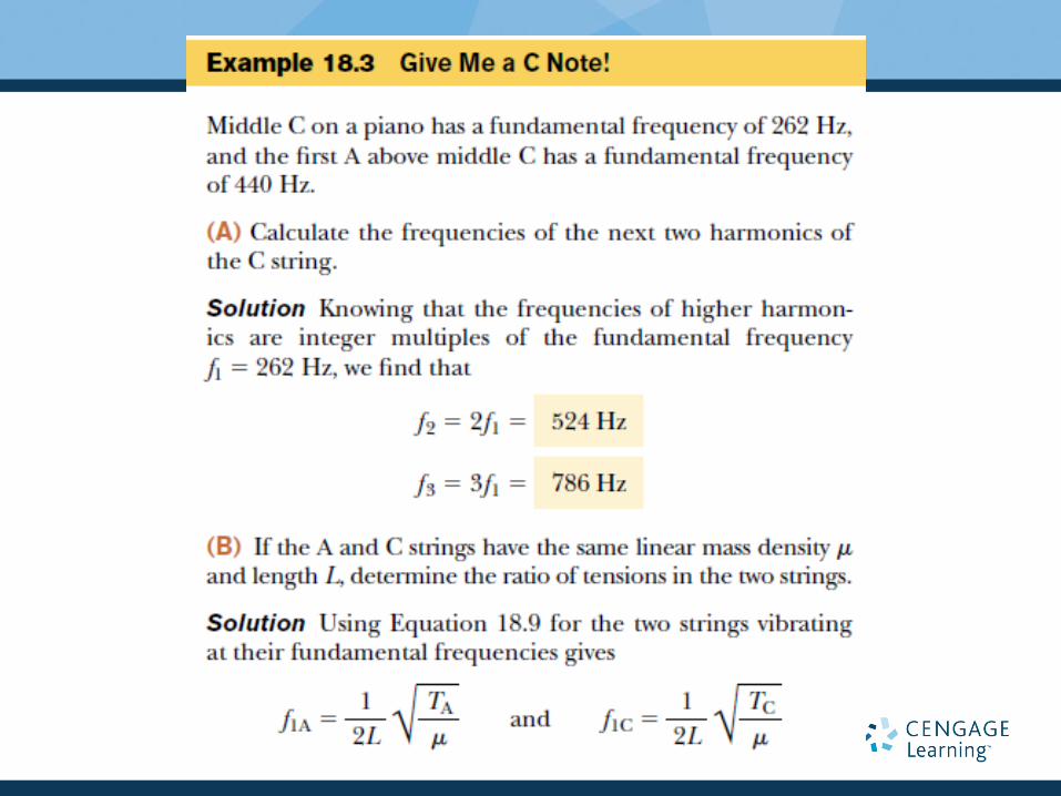
Musical Note of a String

The musical note is defined by its fundamental frequency.

The frequency of the string can be changed by changing either its length or its

tension.

Section 18.3

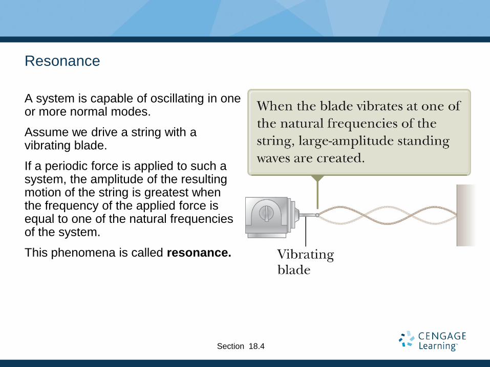
Resonance

A system is capable of oscillating in one or more normal modes.

Assume we drive a string with a vibrating blade.

If a periodic force is applied to such a system, the amplitude of the resulting motion of the string is greatest when the frequency of the applied force is equal to one of the natural frequencies of the system.

This phenomena is called resonance.

Section 18.4

Resonance,

Because an oscillating system exhibits a large amplitude when driven at any of its

natural frequencies, these frequencies are referred to as resonance frequencies.

If the system is driven at a frequency that is not one of the natural frequencies, the

oscillations are of low amplitude and exhibit no stable pattern.

Resonance occurs when a system is able to store and easily transfer energy between

two or more different storage modes .However, there are some losses from cycle to

cycle, called damping. When damping is small, the resonant frequency is

approximately equal to the natural frequency of the system, which is a frequency of

unforced vibrations. Some systems have multiple, distinct, resonant frequencies.

Resonance phenomena occur with all types of vibrations or waves: there

is mechanical resonance, acoustic resonance, electromagnetic resonance, nuclear

magnetic resonance(NMR), electron spin resonance (ESR) and resonance of

quantum wave functions. Resonant systems can be used to generate vibrations of a

specific frequency (e.g., musical instruments),

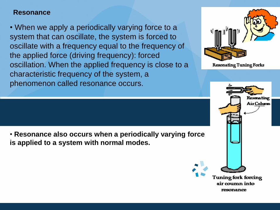
Resonance

• When we apply a periodically varying force to a

system that can oscillate, the system is forced to

oscillate with a frequency equal to the frequency of

the applied force (driving frequency): forced

oscillation. When the applied frequency is close to a

characteristic frequency of the system, a

phenomenon called resonance occurs.

• Resonance also occurs when a periodically varying force

is applied to a system with normal modes.

•of the applied

force is close to one of normal modes of the system,

resonance

occurs.

The sound waves generated by the

fork are reinforced when the length

of the air column corresponds to one

of the resonant frequencies of the

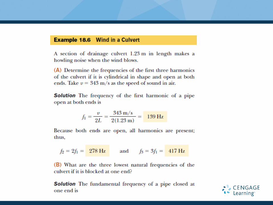
tube. Suppose the smallest value of

L for which a peak occurs in the

sound intensity is 9.00 cm.

Problem

Resonance

Lsmalles t= 9.00 cm

(a) Find the frequency of the

tuning fork.

-1 2

11 345 m.s 9.00 10 mn v L

1 2

1

345 Hz 985 Hz

4 4(9.00 10

vf

L

(b) Find the wavelength and the next two water levels giving resonance.

2

14 4(9.00 10 ) m 0.360 mLl

m. 450.02/ m, 270.02/ 2312 ll LLLL

Beats and interference

Wave interference is the phenomenon that occurs when two waves meet while

traveling along the same medium. The interference of waves causes the medium

to take on a shape that results from the net effect of the two individual waves

upon the particles of the medium.

if two upward displaced pulses having the same shape meet up with one another

while traveling in opposite directions along a medium, the medium will take on

the shape of an upward displaced pulse with twice the amplitude of the two

interfering pulses. This type of interference is known as constructive

interference

If an upward displaced pulse and a downward displaced pulse having the same

shape meet up with one another while traveling in opposite directions along a

medium, the two pulses will cancel each other's effect upon the displacement of

the medium and the medium will assume the equilibrium position. This type of

interference is known as destructive interference

The diagrams below show two waves - one is blue and the other is red -

interfering in such a way to produce a resultant shape in a medium; the

resultant is shown in green. In two cases (on the left and in the middle),

constructive interference occurs and in the third case (on the far right,

destructive interference occurs.

An animation below shows two sound waves interfering constructively in order to produce very large oscillations in pressure at a variety of anti-nodal locations. Note that compressions are labeled with a C and rarefactions are labeled with an R.

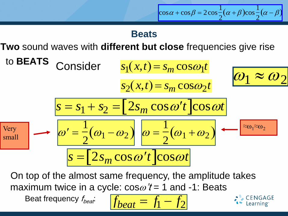
Beats

Two sound waves with different but close frequencies give rise

to BEATS s1 x,t sm cosw1tConsider

s2 x,t sm cosw2tw1 w2

s s1 s2 2sm cos w t coswt

cos cos 2cos1

2 cos

1

2

w 1

2w1 w2 Very

small w

1

2w1 w2

≈w1≈w2

s 2sm cos w t coswt

On top of the almost same frequency, the amplitude takes

maximum twice in a cycle: cosw’t = 1 and -1: Beats Beat frequency fbeat: fbeat f1 f2

Sum and Difference Frequencies

When you superimpose two sine waves of different frequencies, you get components at

the sum and difference of the two frequencies. This can be shown by using a sum

rule from trigonometry. For equal amplitude sine waves

The first term gives the phenomenon of beats with a beat frequency equal to the

difference between the frequencies mixed. The beat frequency is given by

since the first term above drives the output to zero (or a minimum for unequal

amplitudes) at this beat frequency. Both the sum and difference frequencies are

exploited in radio communication.

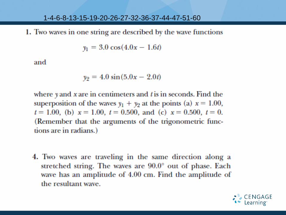
1-4-6-8-13-15-19-20-26-27-32-36-37-44-47-51-60