probability distributions

Probability Distributions

Anthony J. Evans Associate Professor of Economics, ESCP Europe

www.anthonyjevans.com

London, February 2015

(cc) Anthony J. Evans 2015 | http://creativecommons.org/licenses/by-nc-sa/3.0/

Objectives

After attending this lecture, the student will be able to:

–  Develop an intuitive grasp of probability distributions and be able to read tables

–  Distinguish between the Normal, Binomial and Poisson distributions

–  Understand the Central Limit Theorem, and the conditions under which it holds

2

Outline

•  The Normal Distribution –  The Standard Normal Distribution –  The Central Limit Theorem

•  The Binomial Distribution •  The Poisson Distribution

3

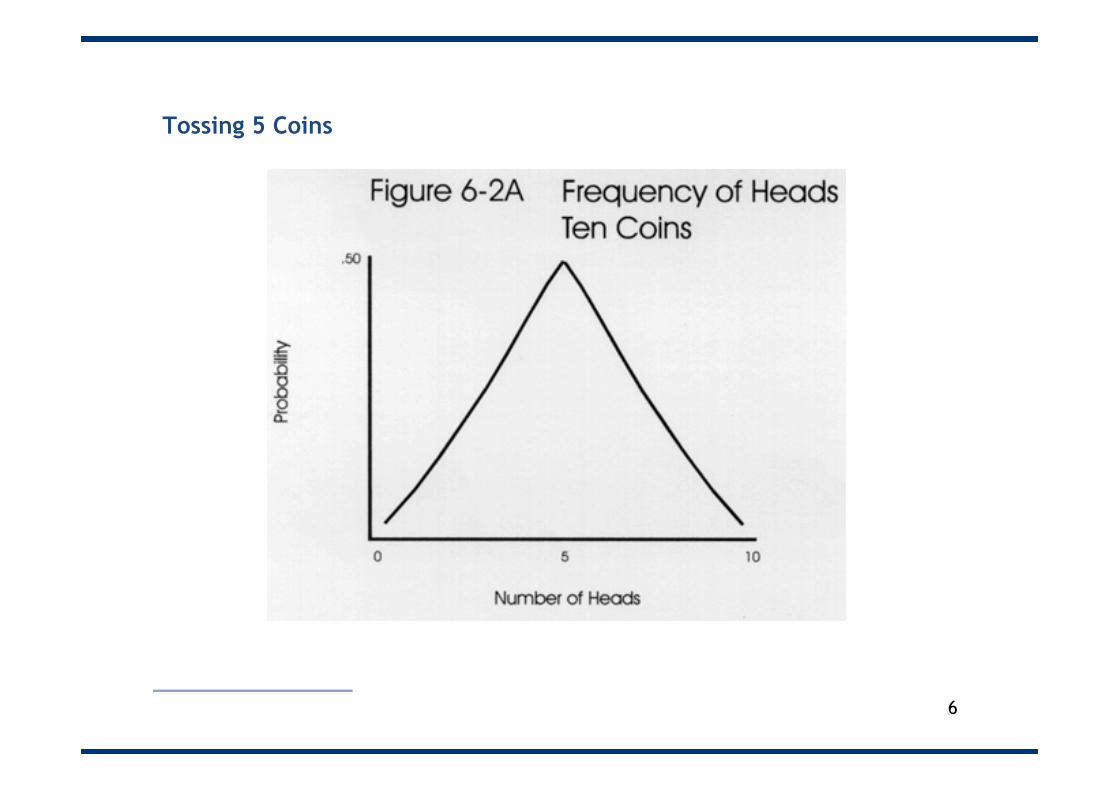
Tossing 5 Coins

•  We know the distribution – it will range from 0 to 5, and we can calculate the probabilities

•  If we toss the coin more than 20 times there is more uncertainty about how many heads well see, but we still have a fully specified probability distribution

4

Tossing 5 Coins

5

Tossing 5 Coins

6

Tossing 5 Coins

7

The Normal Distribution

•  Normal distributions have the same general shape –  Symmetrical about the mean –  Concentrated more in the middle than the tails

•  Mean = mode = median •  The area under the curve is always the same •  The position depends upon

–  the mean (µ) –  the standard deviation (σ)

Carl Gauss on the 10 Deutsch Mark

8

Outline



9

The Standard Normal Distribution

•  The standard normal distribution is a particular normal distribution defined as: –  the mean (µ) = 0 –  the variance (σ^2) = 1

•  Ties into a Z test (used for calculating outliers) –  We can convert any normal distribution to a standard

normal distribution by calculating each z value

σµ−

= ixZExample A test has a mean of 50 and a standard deviation of 10. If Albert’s test score is 70, what is his z score?

10

€

X ~ N(0,12)

Remember, StDev = σ; VAR = σ^2


•  The standard normal distribution is a particular normal distribution defined as: –  the mean (µ) = 0 –  the variance (σ^2) = 1

•  Ties into a Z test (used for calculating outliers) –  We can convert any normal distribution to a standard

normal distribution by calculating each z value

σµ−

= ixZExample A test has a mean of 50 and a standard deviation of 10. If Albert’s test score is 70, what is his z score?

11

€

X ~ N(0,12)

Remember, StDev = σ; VAR = σ^2

Normal distribution

Standard deviations from the mean s

-4 -3 -2 -1 mean 1 2 3 4

Prob

abili

ty

Basic properties

• Mean = mode = median

• 68.2% of the data (area under the curve) lie between -s and +s

• 95.4% of the data (area under the curve) lie between -2s and +2s

• 99.7% of the data (area under the curve) lie between -3s and +3s

• These ± s ranges are called confidence intervals, e.g., the 95% confidence interval is ± 2s around the mean. For population and large sample data, these confidence intervals generally work even if the population is non-normally distributed (m)


12

€

X ~ N(0,12)

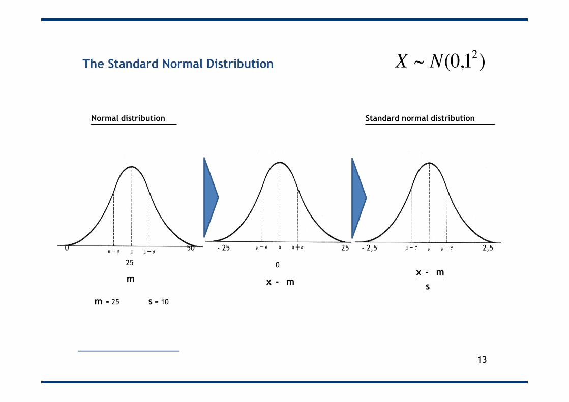
0

Normal distribution Standard normal distribution

x - m s x - m m

- 25 25 - 2,5 2,5

25

0 50

m = 25 s = 10

13


€

X ~ N(0,12)

68% of values are within 1σ of µ

99.7% of values are within 3σ of µ

95% of values are within 2σ of µ

The normal distribution and the 68-95-99.7 rule

14

Why are 95% of values within 2s of the mean?

15

Why are 95% of values within 2s of the mean?

16

2

0.02275

0.02275

- 2

0.954

More precision – what is the Z score associated with 95%?

17

1.96

0.025

0.025

- 1.96

Looking for 0.025

18

Outline



19

The Central Limit Theorem

•  As the sample size increases the distribution of the mean of a random sample approaches a normal distribution with mean µ and standard deviation σ/√n

•  For large enough samples (n>30), we can use the Normal

distribution to analyse the results

),(N

x ributionNormalDistσ

µ≈

20

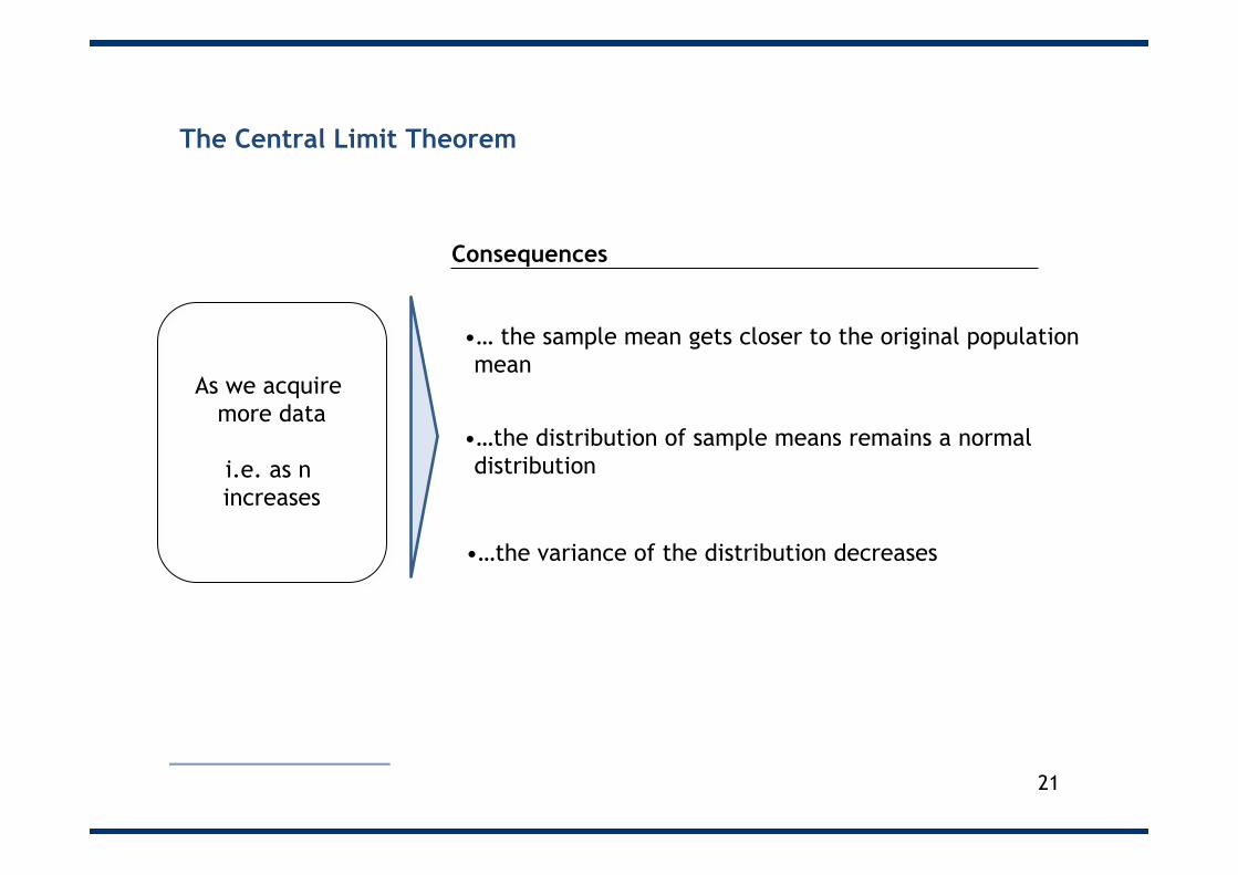
As we acquire more data

i.e. as n increases

• … the sample mean gets closer to the original population mean

• …the distribution of sample means remains a normal distribution

• …the variance of the distribution decreases

Consequences

The Central Limit Theorem

21

Outline



22

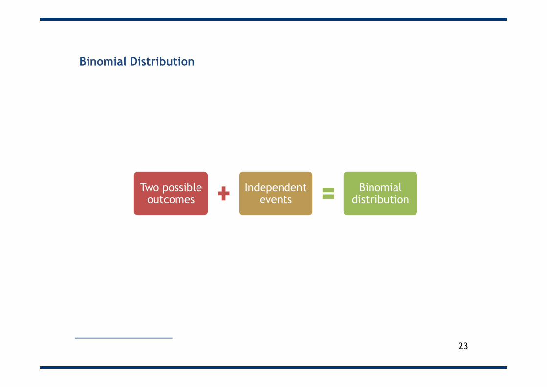
Binomial Distribution

Two possible outcomes

Independent events

Binomial distribution

23

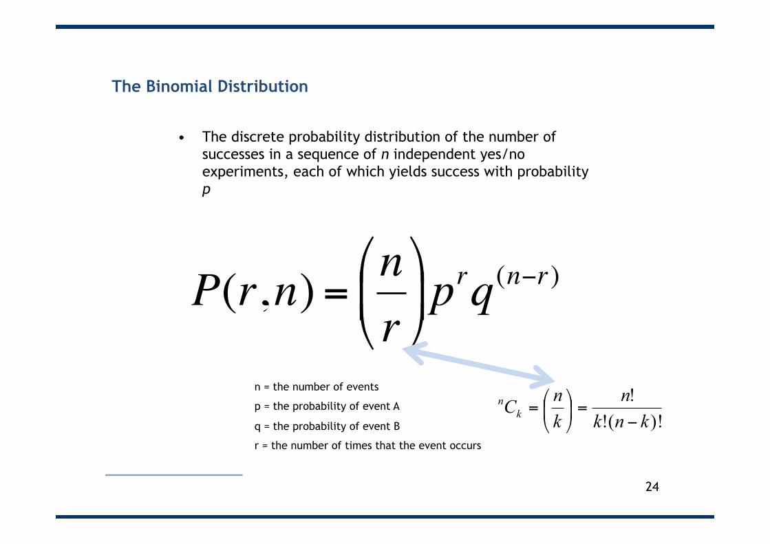
The Binomial Distribution

•  The discrete probability distribution of the number of successes in a sequence of n independent yes/no experiments, each of which yields success with probability p

€

P(r,n) =nr"

# $ %

& ' prq(n−r)

n = the number of events

p = the probability of event A

q = the probability of event B

r = the number of times that the event occurs

24

)!(!!knk

nknCk

n

−=⎟

⎠

⎞⎜⎝

⎛=

The Binomial Distribution: Example

•  If one-in-five items coming off a machine are defective, what is the probability of three defectives in a sample of 10 items?

•  For P(3,10) = 120*(0.203)*(0.807)

= 20.13%

n = 10

p = 0.20

q = 0.80


p, n, and r can be put into a Binomial Table

25

€

P(r,n) =nr"

# $ %

& ' prq(n−r)

€

103

"

# $

%

& ' =

10!3!7!


•  If one-in-five items coming off a machine are defective, what is the probability of three defectives in a sample of 10 items?

•  For P(3,10) = 120*(0.203)*(0.807)

= 20.13%

n = 10

p = 0.20

q = 0.80



26

€

P(r,n) =nr"

# $ %

& ' prq(n−r)

€

103

"

# $

%

& ' =

10!3!7!

27

0.3222-0.1209=0.2013


•  If one-in-five items coming off a machine are defective, what is the probability of three or more defectives in a sample of 10 items?

•  For P(0,10) = 1*(0.200)*(0.8010) = 0.1073

•  For P(1,10) = 10*(0.201)*(0.809)

•  For P(2,10) = 45*(0.202)*(0.808)

•  P(>=3) = 1 – [P(2)+P(1)+P(0)]

= 1 – 0.678

= 32.2%

n = 10

p = 0.20

q = 0.80



28

€

P(r,n) =nr"

# $ %

& ' prq(n−r)


•  If one-in-five items coming off a machine are defective, what is the probability of three or more defectives in a sample of 10 items?

•  For P(0,10) = 1*(0.200)*(0.8010) = 0.1073

•  For P(1,10) = 10*(0.201)*(0.809)

•  For P(2,10) = 45*(0.202)*(0.808)

•  P(>=3) = 1 – [P(2)+P(1)+P(0)]

= 1 – 0.678

= 32.2%

n = 10

p = 0.20

q = 0.80



29

€

P(r,n) =nr"

# $ %

& ' prq(n−r)

30

0.3222

Outline



31

Poisson distribution

Fixed period of time

Recurring interval

Poisson distribution

32

The Poisson Distribution

•  “expresses the probability of a number of events occurring in a fixed period of time if these events occur with a known average rate, and are independent of the time since the last event”

•  The probability of their being k occurrences is given as:

•  e is a constant (the base of the natural logarithm) = 2.71828

•  k! is a factorial of k* •  λ is the expected number of occurrences that occur during

a given interval

* n! is the product of all +ve integers less than or equal to n. e.g. 5! = 5*4*3*2*1 33

€

f (k;λ) =e−λλk

k!

λ: ” Lamda”

•  λ is the expected number of occurrences that occur during a given interval

•  Example: the event occurs every 5 minutes, and you’re interested in how often they’d occur over 20 minutes

•  What’s λ? λ = 20/5

= 4

34

λ: ” Lamda”

•  λ is the expected number of occurrences that occur during a given interval

•  Example: the event occurs every 5 minutes, and you’re interested in how often they’d occur over 20 minutes

•  What’s λ? λ = 20/5

= 4

35

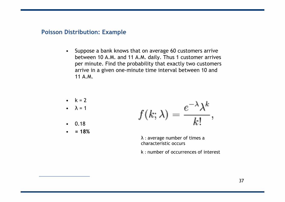
Poisson Distribution: Example

•  Suppose a bank knows that on average 60 customers arrive between 10 A.M. and 11 A.M. daily. Thus 1 customer arrives per minute. Find the probability that exactly two customers arrive in a given one-minute time interval between 10 and 11 A.M.

•  k = 2 •  λ = 1

•  0.18 •  = 18%

λ : average number of times a characteristic occurs

k : number of occurrences of interest

36


•  Suppose a bank knows that on average 60 customers arrive between 10 A.M. and 11 A.M. daily. Thus 1 customer arrives per minute. Find the probability that exactly two customers arrive in a given one-minute time interval between 10 and 11 A.M.

•  k = 2 •  λ = 1

•  0.18 •  = 18%



37


•  A company receives an average of three calls per 5 minute period of the working day

•  What is the probability of answering 2 calls in any given 5-minute interval?

•  k = 2 •  λ = 3

•  0.22 •  = 22%



λ, and k can be put into a Poisson Table

38 Also referred to as ‘Queuing Theory’



•  What is the probability of answering 2 calls in any given 5-minute interval?

•  k = 2 •  λ = 3

•  0.22 •  = 22%



λ, and k can be put into a Poisson Table

39 Also referred to as ‘Queuing Theory’

40

0.8009-0.5768=0.2241



•  What is the probability of answering 5 calls or more in any given 5-minute interval?

41

42

0.1847

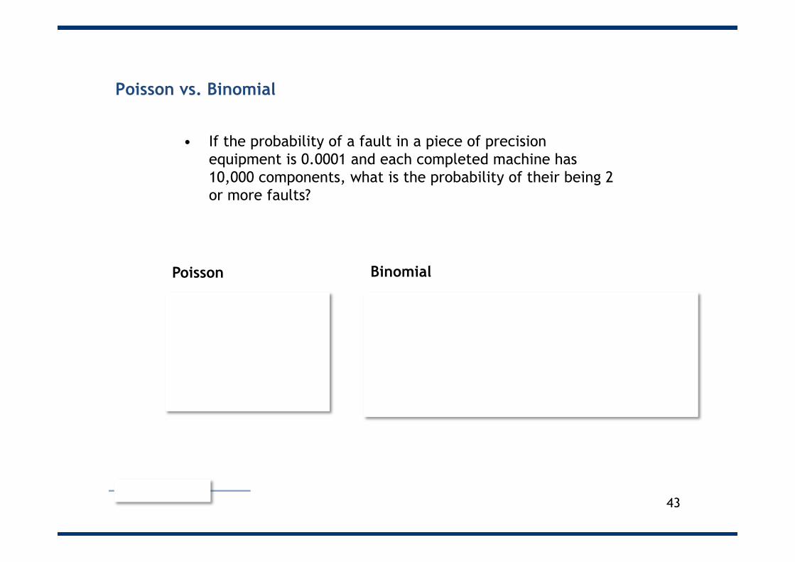
Poisson vs. Binomial

•  If the probability of a fault in a piece of precision equipment is 0.0001 and each completed machine has 10,000 components, what is the probability of their being 2 or more faults?

43 CS, p.242

Poisson P(0) = e-1 = 0.3679 P(1) = e-1 = 0.3679 P(0)+P(1) = 0.7358 P(>1 )= 1-0.7358 =0.2642

Binomial P(0) = 1*0.000010*0.999910,000 = 0.3679 P(1) = 10,000*0.000011*0.99999,999 = 0.3679 P(0)+P(1) = 0.7358 P(>1) = 1-0.7358 =0.2642

Poisson vs. Binomial

•  If the probability of a fault in a piece of precision equipment is 0.0001 and each completed machine has 10,000 components, what is the probability of their being 2 or more faults?

44 CS, p.242

Poisson P(0) = e-1 = 0.3679 P(1) = e-1 = 0.3679 P(0)+P(1) = 0.7358 P(>1 )= 1-0.7358 =0.2642

Binomial P(0) = 1*0.000010*0.999910,000 = 0.3679 P(1) = 10,000*0.000011*0.99999,999 = 0.3679 P(0)+P(1) = 0.7358 P(>1) = 1-0.7358 =0.2642

Summary

•  Probability distributions are the basis for inferential statistics since they demonstrate the characteristics of a dataset

•  It’s easy to practice textbook examples (which is highly recommended) but also important to put into a practical setting

45

APPENDIX

The normal distribution

47

Binomial probabilities

1 3 5 7 9 11 13 15 17 19 21

Number of "successes"

0,00

0,02

0,04

0,06

0,08

0,10

0,12

0,14

0,16

0,18

Remark: The normal distribution is a good approximation of a binomial distribution when n is large and p is not too small or too large, typically np>5 and nq>5

PROBABILITY OF THE RESULT OF A COIN TOSS (HEAD OR FACE)

Binomial Distribution: Graph

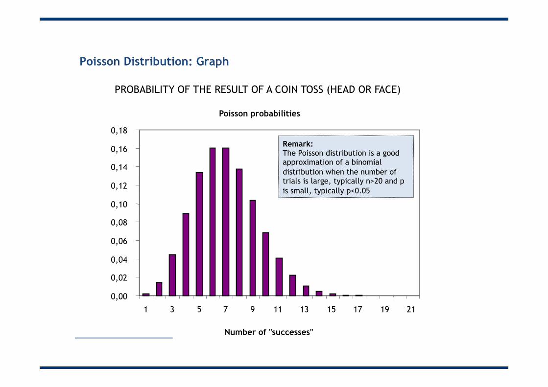
Poisson probabilities

0,00

0,02

0,04

0,06

0,08

0,10

0,12

0,14

0,16

0,18

1 3 5 7 9 11 13 15 17 19 21

Number of "successes"

Remark: The Poisson distribution is a good approximation of a binomial distribution when the number of trials is large, typically n>20 and p is small, typically p<0.05

Poisson Distribution: Graph

PROBABILITY OF THE RESULT OF A COIN TOSS (HEAD OR FACE)

•  This presentation forms part of a free, online course on analytics

•  http://econ.anthonyjevans.com/courses/analytics/

50

probability distributions

Data & Analytics