publisher - bg.pg.gda.pl
TRANSCRIPT

Address of Publisher & Editor's Office :
GDAŃSK UNIVERSITYOF TECHNOLOGY
Facultyof Ocean Engineering
& Ship Technology
ul. Narutowicza 11/1280-952 Gdańsk, POLAND
tel.: +48 58 347 13 66fax : +48 58 341 13 66
e-mail : [email protected]
Account number :BANK ZACHODNI WBK S.A.
I Oddział w Gdańsku41 1090 1098 0000 0000 0901 5569
Editorial Staff :Tadeusz Borzęcki Editor in Chief
e-mail : [email protected]ław Wierzchowski Scientific Editor
e-mail : [email protected] Michalski Editor for review matters
e-mail : [email protected] Kniat Editor for international re la tions
e-mail : [email protected] Kempa Technical Editor
e-mail : [email protected] Bzura Managing Editor
e-mail : [email protected] Spigarski Computer Design
e-mail : [email protected]
Domestic price :single issue : 20 zł
Prices for abroad :single issue :
- in Europe EURO 15- overseas US$ 20
ISSN 1233-2585
POLISH MARITIME RESEARCH
in internetwww.bg.pg.gda.pl/pmr/pmr.php
PUBLISHER :
3 JAN P. MICHALSKI Parametric method for determination of motion characteristics of underwater vehicles, applicable in preliminary designing
11 ZBIGNIEW SEKULSKI Structural weight minimization of high speed vehicle-passenger catamaran by genetic algorithm
24 ROOZBEH PANAHI, MEHDI SHAFIEEFAR Application of Overlapping Mesh in Numerical Hydrodynamics
34 TADEUSZ KORONOWICZ, ZBIGNIEW KRZEMIANOWSKI, TERESA TUSZKOWSKA, JAN A. SZANTYR A complete design of ducted propellers using the new computer system
40 MAREK DZIDA, JANUSZ MUCHARSKI On the possible increasing of efficiency of ship power plant with the system combined of marine diesel engine, gas turbine and steam turbine in case of main engine cooperation with the gas turbine fed in parallel and the steam turbine
45 JERZY ŚWIRYDCZUK Two vortex interaction patterns in a turbine rotor
54 JANUSZ GARDULSKI Vibration and noise minimisation in living and working ship compartments
60 JERZY KOWALSKI ANN based evaluation of the NOx concentration in the exhaust gas of a marine two-stroke diesel engine
67 JERZY KABACIŃSKI, BOGUSZ WIŚNICKI Accuracy analysis of stowing computations for securing non-standard cargoes on ships according to IMO CSS Code
72 RENATA DOBRZYŃSKA Selection of outfitting and decorative materials for ship living accommodations from the point of view of toxic hazard in the initial phase of fire progress
CONTENTS
POLISH MARITIME RE SE ARCHNo 2(60) 2009 Vol 16

POLISH MARITIME RESEARCH is a scientific journal of worldwide circulation. The journal ap pe ars as a quarterly four times a year. The first issue of it was published in September 1994. Its main aim is to present original, innovative scientific ideas and Research & Development achie ve ments in the field of :
Engineering, Computing & Technology, Mechanical Engineering,
which could find applications in the broad domain of maritime economy. Hence there are published papers which concern methods of the designing, manufacturing and operating processes of such technical objects and devices as : ships, port equ ip ment, ocean engineering units, underwater vehicles and equipment as
well as harbour facilities, with accounting for marine environment protection.The Editors of POLISH MARITIME RESEARCH make also efforts to present problems dealing with edu ca tion of engineers and scientific and teaching personnel. As a rule, the basic papers are sup ple men ted by information on conferences , important scientific events as well as co ope ra tion in carrying out in ter na-
tio nal scientific research projects.
Editorial
Scientific BoardChairman : Prof. JERZY GIRTLER - Gdańsk University of Technology, PolandVice-chairman : Prof. ANTONI JANKOWSKI - Institute of Aeronautics, Poland
Vice-chairman : Prof. MIROSŁAW L. WYSZYŃSKI - University of Birmingham, United Kingdom
Dr POUL ANDERSENTechnical University
of DenmarkDenmark
Dr MEHMET ATLARUniversity of Newcastle
United Kingdom
Prof. GÖRAN BARKChalmers Uni ver si ty
of TechnologySweden
Prof. SERGEY BARSUKOVArmy Institute of Odessa
Ukraine
Prof. MUSTAFA BAYHANSüleyman De mi rel University
Turkey
Prof. MAREK DZIDAGdańsk University
of TechnologyPoland
Prof. ODD M. FALTINSENNorwegian University
of Science and TechnologyNorway
Prof. PATRICK V. FARRELLUniversity of Wisconsin
Madison, WI USA
Prof. WOLFGANG FRICKETechnical UniversityHamburg-Harburg
Germany
Prof. STANISŁAW GUCMAMaritime University of Szczecin
Poland
Prof. ANTONI ISKRAPoznań University
of TechnologyPoland
Prof. JAN KICIŃSKIInstitute of Fluid-Flow Machinery
of PASciPoland
Prof. ZYGMUNT KITOWSKINaval University
Poland
Prof. JAN KULCZYKWrocław University of Technology
Poland
Prof. NICOS LADOMMATOSUniversity College London
United Kingdom
Prof. JÓZEF LISOWSKIGdynia Ma ri ti me University
Poland
Prof. JERZY MATUSIAKHelsinki Uni ver si ty
of TechnologyFinland
Prof. EUGEN NEGRUSUniversity of Bucharest
Romania
Prof. YASUHIKO OHTANagoya Institute of Technology
Japan
Dr YOSHIO SATONational Traffic Safety
and Environment LaboratoryJapan
Prof. KLAUS SCHIERUniversity of Ap plied Sciences
Germany
Prof. FREDERICK STERNUniversity of Iowa,
IA, USA
Prof. JÓZEF SZALABydgoszcz Uni ver si ty
of Technology and AgriculturePoland
Prof. TADEUSZ SZELANGIEWICZTechnical University
of SzczecinPoland
Prof. WITALIJ SZCZAGINState Technical University
of KaliningradRussia
Prof. BORIS TIKHOMIROVState Marine University
of St. Pe ters burgRussia
Prof. DRACOS VASSALOSUniversity of Glasgow
and StrathclydeUnited Kingdom
3POLISH MARITIME RESEARCH, No 2/2009
INTRODUCTION
Underwater vehicles serve to carry out scientific research; they find applications in offshore industry and to military important purposes. Variety of their operational applications is associated with a wide range of functional demands including those regarding movement properties. Selection of both geometrical configuration of a vehicle and its propulsion system greatly depends on demands put to its motion. The presented method is intended for preliminary approximate prediction of kinematic and dynamic properties of motion of autonomous underwater vehicles on the basis of set of technical parameters which identify designed vehicle already in early design stages. Research on underwater vehicles belongs to the area of interest of many research centers all over the world. This can be exemplified by multi-year commitment of Massachusetts Institute of Technology to realization of comprehensive research carried out in the frame of Sea Grant project, or that realized by Virginia Polytechnic Institute and State University, as well as by many other scientific institutions whose list can be found in [1].
In state of immersion, the remotely operated vehicle (ROV), or also autonomous underwater vehicle (AUV) can perform motion of six degrees of freedom, like airplane in flight. Differential equations which describe such motion – due to large number of independent variables, their high order, non-linearity and coupling as well as due to complex boundary conditions – constitute a difficult mathematical problem [2, 3, 4],
applied in the stage of design verification calculations. In the practical preliminary designing of underwater vehicles of complex forms resulting from their functions it is necessary to make preliminarily use of parametric design methods based on such mathematical models, that leads – at allowable simplifications – to efficient determination of acceptable approximate solutions.
When operation of an underwater vehicle consists mainly in moving with constant speed as in the case of classical transport ships then the designing of its hull form and propulsion system is based on hull steady-motion resistance characteristics. However if its operation is inherently associated with frequent changes of motion speed in order to realize vehicle’s functions (underwater operations and working tasks) then to use dynamic resistance-propulsion characteristics in unsteady motion is necessary in its designing, that constitutes a non-classical task of ship design theory.
The problem presented in this paper concerns elaboration of a method applicable to the designing of underwater vehicles in the case when design assumptions contain requirements dealing with kinematic and dynamic parameters of designed vehicle, e.g. such as the following: � to cover a given distance within a set time� to develop a required speed within a set time� to develop a required speed along a set distance.
Concept of the method is based on selection of a form of planar motion equation for a vehicle which moves in two
Parametric method for determination of motion characteristics of underwater vehicles,
applicable in preliminary designing
Jan P. Michalski, Assoc. Prof.Gdańsk University of TechnologyPolish Naval University
ABSTRACT
This paper describes a method for preliminary designing the autonomous underwater vehicles (AUV), especially useful in the case when requirements concerning kinematic and dynamic parameters of vehicle motion are given in design assumptions. Concept of the method is based on dynamic equations which describe vehicle planar motion in vertical and horizontal directions, resulting from action of screw propellers or water ballast, respectively. The motion equations were determined by applying simplifications concerning both geometrical description of vehicle’s form and flow phenomena. Their solutions were obtained in the form of closed analytical expressions which are both of cognitive and practical
merits as they can serve to assess influence of vehicle’s design parameters on its motion characteristics and simultaneously are convenient to formulate design optimization problems. Application of the method was illustrated by the attached examples dealing with determination of kinematic and dynamic characteristics
of motion of the vehicle „Scylla” of set geometrical configuration and propulsion parameters. Keywords: underwater vehicles; preliminary designing method
POLISH MARITIME RESEARCH 2(60) 2009 Vol 16; pp. 3-1010.2478/v10012-008-0016-6

4 POLISH MARITIME RESEARCH, No 2/2009
orthogonal directions: horizontal or vertical. Usefulness of the method for engineering applications can be assessed by examining fulfillment of the following criteria:� to be capable of predicting the kinematic and dynamic
characteristics of underwater vehicles� to be applicable to preliminary designing the underwater
vehicles identified by a scarce set of numerical design parameters
� to be applicable to realizing research tasks intended for gaining knowledge on ranges of permissible values of design parameters of underwater vehicles, and to have practical application merits.
Vehicle motion is forced by thrust force generated by screw propellers, or by resultant of vehicle buoyancy force and its weight dependent on a chosen amount of water ballast. Application of the method is illustrated by the attached examples which concern assessment of influence of values of design parameters of geometrical configuration as well as propulsion system’s parameters of a vehicle on its motion characteristics.
INVESTIGATION METHOD AND AIM OF THE WORK
The applied investigation method consists in formulation of equations of underwater vehicle motion, expressed by means of its main design parameters, determination of their analytical solutions, as well as elaboration of computational algorithms in order to perform test calculations. Mathematical model of vehicle motion was elaborated by assuming simplifications which concerned both vehicle geometrical form description and flow phenomena. Expressions describing relations between object’s geometrical parameters and forces exerted onto vehicle, were determined on the basis of theoretical knowledge as well as results of experimental investigations, taken from the subject-matter literature sources [5, 6].
Motion equations in their initial form express equilibrium of forces acting onto vehicle, i.e. inertia forces of vehicle mass inclusive of added water mass, thrust of propellers, vehicle resistance, its weight and buoyancy. Values of the forces depend on vehicle parameters, water environment features, values of vehicle speed and acceleration. So determined dynamic characteristics of motion are functions dependent on time, displacement, speed, acceleration and design parameters of vehicle.
Their solutions determined in the form of close analytical relations, have both cognitive and practical merits as they make it possible to investigate in a simple and straight way influence of vehicle design parameters on its motion characteristics; moreover they are convenient for formulation of design optimization problems useful to computer aided preliminary designing. Summing up, the aim of the work in question consists in elaboration of a practical engineering method applicable to the preliminary designing of autonomous underwater vehicles of given set motion parameters – performed by means of analytically expressed vehicle motion characteristics. Simplifications of the method, based on engineering practice, concern geometrical form description, choice of directions of vehicle motion, omittment of less important forces; and, they particularly concern the following: � unsteady rectilinear motion described by non-linear
differential equations� application of hypothesis on invariability of vortex forces
in steady and unsteady motions� omittment of action of lift forces
� validity of the principle of superposition of forces� constant values of physical parameters (water density and
viscosity).
Vehicle’s resistance depends on a kind of flow around its elements, which can be locally either laminar or turbulent, with or without separation of flow; the variety of flow kinds makes it difficult to provide unambiguous mathematical description of the phenomena on the ground of theoretical knowledge, that forces to introduce simplifying assumptions. Wave-generated resistance is negligible as operational range of vehicle is sufficiently far from water surface. Flow phenomena such as formation of boundary layer, viscosity resistance, pressure resistance, flow separation, generation of lift forces, or cavitation are analogous to those in the case of classical ships but they occur at different values of Reynold’s number and pressure.
MATHEMATICAL MODEL OF THE PROBLEM
Vehicle’s motion is described in the motionless rectangular coordinate system of z-axis pointing the gravity force direction, and horizontal x-axis, as shown in Fig. 1.
Fig. 1. The coordinates system and position of the vehicle respective to directions of its motion
The relationship of inertia force and external forces acting on vehicle of the component masses Mj, in unsteady rectilinear motion, is expressed as follows:
(1)
If vehicle motion is directed along z-axis then balance of forces is given by the equation:
(2)
where the following case is considered:
(3)
If vehicle motion is directed along x-axis then balance of forces is given by the equation:
(4)
5POLISH MARITIME RESEARCH, No 2/2009
(12)
The total vehicle resistance is hence expressed as follows:
(13)
The resistance coefficient αs takes value respectively αx or αz depending on vehicle geometrical parameters and a considered direction of its motion.
SPEED-DEPENDENT CHARACTERISTICS OF VEHICLE DISPLACEMENTS TIME
Under the presented simplifying assumptions, rectilinear motion along s-axis, of a vehicle which moves with a speed corresponding with moderate values of Reynolds number, is described by the non-linear ordinary differential equation of constant coefficients:
where the following case is considered:
(5)
SIMPLIFYING ASSUMPTIONS
In the preliminary design stage, vehicle is identified by the vector of main design parameters, , and a set of attributes which describe geometrical configuration of vehicle form. Such identification is supplemented with a set of physical constants and data concerning characteristics of propellers and resistance characteristics of bodies of simple geometrical forms. It is assumed that at the considered vehicle motions the resistance and thrust forces are collinear, that is necessary to perform rectilinear motion.
Value of the force:
which accelerates mass of water surrounding the vehicle, has been replaced by value of the force which, to a determined mass of water, , (the so-called added mass of water), gives acceleration equal to that of the vehicle itself:
(6)
Depending on the direction of vehicle motion, , the mass ∆Ms takes the value proportional to the vehicle mass:
(7)
The propelling force TN generated by m – propellers whose bollard thrust is equal to To, at variable velocity of water inflow to the propellers, can be approximated by the relationship:
(8)
Is difficult to express vehicle resistance value by an analytical relation dependent on vehicle form because of its geometrical configuration which is complex, open-work and
multiply-connected. Moreover, the difficulty results from the fact that object resistance values in steady and unsteady motion at the same speed are different, as indicated by results of experimental tests [7].
Simplification of the method concerning the determination of resistance, consists in assumption of hypothesis on invariability of vortex forces in steady and unsteady motions, that is justified in the case of flows without separation, i.e. occurring in the range of moderate values of Reynolds number and for streamline bodies. Ambiguouity with respect to a kind of flow around vehicle elements causes that for practical application of the method some calibration of the coefficients (or functions) ks as well as ξs is required.
The total vehicle resistance Rs was expressed as the sum of the viscous resistance Rv and the pressure resistance Rp of vehicle elements, determined by using the formulae given in [2, 3], as well as ITTC-57 formula. The total vehicle resistance Rs in motion in s-direction (along x-axis or z-axis) follows superposition without taking into account interferential influence of vehicle elements:
(9)
The viscosity resistance was expressed by the friction resistance Rf,s and the form coefficients ks, by summing the resistance values of particular vehicle elements of the reference surface areas Ωi:
(10)
The friction resistance coefficient was determined by the ITTC-57 formula:
(11)
where the velocity vs was assumed equal to a half of zero-thrust velocity of propellers.
The pressure resistance coefficient concerning the slender elements of vehicle was determined in compliance with the formulae given in [3]:

6 POLISH MARITIME RESEARCH, No 2/2009
(14)
On simplification of the description with the use of the following substitutions:
(15)
the equation takes the form:
(16)
which can be transformed to the form of the equation of separated variables:
(17)
The equation can be expressed in the form convenient to integration:
(18)
By denoting as follows:
(19)
the general integral of the equation can be expressed by the function:
(20)
Under the initial condition: if t = 0 then
and on substitution:
(21)
the particular solution of the equation takes the form of the function :
(22)
which represents characteristics of the time t duration after which the vehicle reaches an assumed value of the speed v, counting from the instant when vehicle speed has been equal to vo.
Time-dependent characteristics of speed and acceleration constitutes the dependence of the vehicle speed v on duration time of its motion, expressed by the function :
(23)
Characteristics of the vehicle acceleration is expressed by the derivative with respect to time, :

7POLISH MARITIME RESEARCH, No 2/2009
(24)
SPEED-DEPENDENT CHARACTERISTICS OF DISPLACEMENTS
The equation can be transformed to the form:
(25)
and next, by integrating both its sides, the following relation is obtained:
(26)
The general solution of the equation is the function :
(27)
Under the initial condition: if s = 0 then v = vo, the particular solution takes the form of the characteristics :
(28)
which expresses the relation of the distance (path) covered by the vehicle beginning from the instant whenits speed has been equal to vo till the instant when it reaches the speed v = vo = ∆v.
TIME-DEPENDENT CHARACTERISTICS OF DISPLACEMENTS
By making use of the equation the distance (path) covered during the time t can be expressed by the relation :
(29)
On transformation of the equation to the form convenient to integration:
(30)
the general solution of the equation is obtained in the form of the function :
(31)

8 POLISH MARITIME RESEARCH, No 2/2009
By imposing the initial condition: if t = to then s = 0, the searched particular solution achieves the form of the function:
(32)
The parameter vo which appears in the formulas, determines the vehicle speed in the instant to.The presented relationships express characteristics useful in the designing
of vehicle geometrical configuration and the determining of propulsion system parameters.
EXAMPLES OF APPLICATION OF THE METHOD
Vehicle geometrical configuration
A vehicle of geometrical configuration composed of i = 0, 1, 2, 3... spatial frame rods; j = 0, 1, 2, 3... axially symmetrical slender pontoons; k = 0, 1, 2, 3... equipment elements in the form of plates, discs or cylinders is considered. The vehicle is moved by p = 0, 1, 2, 3... screw propellers, as shown in Fig. 2.
Fig. 2. Draft configuration of the example vehicle „Scylla”
The vehicle „Scylla” is under consideration, its data used to perform example calculations are listed in Tab. 1.
In the example the components of the vector concerning the screw propeller parameters relate to the B.5.60 propeller type: H/Dp = 0.5, KT(J = 0) = 0.25, KQ(J = 0) = 0.025, Jk(T = 0) = 0.55, vk = Jk · np · Dp, where Jk is the propeller zero-thrust advance ratio. For calculations of motion along x-axis the approximate value ξx ≈ 0.25 was assumed, and in the case of motion along z-axis – the value ξz ≈ 0.5.
Simulation of horizontal motion of the vehicle
The problem of determination of kinematic and dynamic motion characteristics of a vehicle having set geometrical configuration and determined propulsion parameters is considered for the case of motion along x-axis. The horizontal motion of the „Scylla” vehicle of the mass displacement D = 1.6 t is produced by thrust of two screw propellers of 0.35 m diameter. The resulting kinematic and dynamic motion characteristics are graphically presented in Fig. 3.
From the obtained results it follows that at the starting-up power of 1 kW delivered to each of the propellers, the vehicle develops the constant speed of ∼ 0.85 m/s after passing the time of 8 s and covering the distance of 6 m by the vehicle. At this constant speed each of the propellers consumes the power of 0.8 kW at the rotational speed of 600 rpm.
Tab. 1. Basic design parameters (i.e. components of the vector x) of the vehicle „Scylla”
Pontoon geometrical descriptionAttribute – spheroids
Np 2 [-] NumberLp 5.00 [m] LengthDp 0.50 [m] DiameterVp 0.65 [m3] VolumeSp 5.58 [m2] Wetted Area
Geometrical description of frame longitudinal elements Attribute – cylinders
Nw 6 [-] NumberLw 5.00 [m] LengthDw 0.10 [m] DiameterVw 0.04 [m3] VolumeSw 1.57 [m2] Wetted Area
Geometrical description of frame transverse elements Attribute – cylinders
Nk 8 [-] NumberLk 1.50 [m] LengthDk 0.05 [m] DiameterVk 0.01 [m3] VolumeSk 0.24 [m2] Wetted Area
Geometrical description of outside equipment Attribute – plates&discs
Nt 2 [-] NumberLt 0.15 [m] LengthDt 0.30 [m] DiameterVt 0.01 [m3] VolumeSt 0.42 [m2] Wetted Area
Parameters of screw propeller of the type B.5.60. H/D = 0.5Nps 2 [-] NumberDs 0.35 [m] DiameterNs var [rpm] Rotational speed
In the case of delivering the starting-up power of 2 kW to each of the propellers their rotational speed increases from 600 rpm to 750 rpm, and the vehicle speed increases to 1 m/s. After steadying the speed, each of the propellers will consume the power of 1.6 kW. The remaining characteristics are presented in Fig. 4.

9POLISH MARITIME RESEARCH, No 2/2009
Fig. 3. Horizontal motion characteristics of the vehicle „Scylla” at the propulsion power of 2x1 kW
Fig. 4. Horizontal motion characteristics of the vehicle„Scylla” at the propulsion power of 2x2 kW
Simulation of vertical motion of the vehicle
In the case of the motion along z-axis the problem of determination of kinematic and dynamic motion characteristics is considered for the vehicle of set geometrical configuration and buoyancy/weight ratio controlled by chosen mass of water ballast. Vertical motion of the vehicle is produced by difference between buoyancy and weight forces of the vehicle without any interference of screw propulsion.
The resulting kinematic and dynamic motion characteristics are graphically presented in Fig. 5. for the case of the surplus of weight over buoyancy, equal to P – W = 0.981 kN, which resulted from taking the water ballast of 0.1 t mass.
Fig. 5. Vertical motion characteristics of the vehicle„Scylla”, resulting from taking the water ballast of 0.1 t mass
In this case the propulsion power is determined by the product of vehicle’s speed and difference of its weight and buoyancy.
CONCLUSIONS
� The presented method is characteristic of simplicity of application and prediction merits, that makes it useful in aiding and performing the preliminary design tasks.
� The method can serve both for computer aided design of underwater vehicles and realization of parametric investigations aimed at determination of relations (e.g. indices) useful in formulating the preliminary design methods for underwater vehicles.
� Parametric structure of the method makes changes in design decisions easier due to simple way of introducing appropriate corrections in order to achieve design solutions of expected operational and technical features of designed vehicle.
� To validate of the method and implement it to engineering design practice, verification and calibration of the coefficients of motion equations by means of experimental tests is required in order to determine their values correlated with various vehicle form configurations.
� The method can be refined by adding available propulsion characteristics (e.g. of ducted propellers) as well as those of vehicle resistance. In particular, the method can be improved by taking into account the phenomena described in [7] as well as influence of high pressure on resistance and propulsion phenomena.
� An initial comparison of the obtained results with the data available from the subject-matter literature, e.g. [1] (comparison of delivered power and predicted vehicle speed values) indicates that the vehicle motion characteristics determined by using the presented method are realistic.
NOMENCLATURE
ks – form coefficient for motion in s-directionm – number of propellersnp – rotational speed of screw propellersv – vehicle speed (v < vk) vo – initial speed of vehiclevk – propeller zero-thrust speedw – wake factorB – water mass acceleration forceCfi, s
– friction resistance coefficient for motion in s-directionD – vehicle buoyancyDp – propeller diameterJk – propeller zero-thrust advance ratioKT – propeller bollard thrust coefficientKQ – propeller bollard torque coefficientMb – water ballast massMj – components of mass of vehicleMo – mass of vehicle with water ballastMp – mass of vehicle without water ballastMs – accelerated massP – vehicle weightRtx – vehicle resistance to motion along x-axisRtz – vehicle resistance to motion along x-axisTo – propeller bollard thrustTN – thrust of propellersV – vehicle volumetric displacementW – vehicle buoyancy forceν – kinematic viscosity coefficient of waterρ – density of waterξs – added water mass coefficient for motion in s-direction
– vector of parameters which describe a vehicle∆Ms – added water massΩj – reference surface areas of vehicle elements.

10 POLISH MARITIME RESEARCH, No 2/2009
BIBLIOGRAPHY
1. http://auvlab.mit.edu/resources/HV-SGT (10.01.2009)2. Fang M.C., et al.: On the Behavior of an Underwater Remotly
Operated Vehicle in a Uniform Current. Marine Technology. Vol. 45, No. 4, 2008
3. Garus J.: Identification of motion parameters of floating objects in operational conditions by using numerical methods (in Polish). Doctor thesis, Polish Naval Academy, Gdynia 1993
4. Żak A.: Identification of dynamic motion of unmanned underwater vehicle in operational conditions (in Polish). Doctor thesis, Polish Naval Academy, Gdynia 2006
5. Hoerner S.F.: Fluid dynamic drag. Published by the Author. 1965
6. Bukowski J.: Fluid Mechanics (in Polish). State Scientific Publishing House (Państwowe Wydawnictwo Naukowe). Warszawa 1976
7. Nikołajew E.P.: A contribution to the problem of acceptance of stationarity hypothesis for assessment of resistance of bodies of bad around-flow (in Polish). 2nd Symposium on Ship Hydromechanics. Application of model tests to ship design. Ship Design and Research Centre, Gdańsk 1974.
CONTACT WITH THE AUTHOR
Assoc. Prof. Jan P. MichalskiFaculty of Ocean Engineering
and Ship TechnologyGdansk University of Technology
Narutowicza 11/1280-952 Gdansk, POLANDe-mail : [email protected]

11POLISH MARITIME RESEARCH, No 2/2009
INTRODUCTION
A primary objective of the ship structural optimization is to find the optimum positions of structural elements, also referred to as topological optimization, shapes (shape optimization) and scantlings (sizing optimization) of structural elements for an objective function subject to constraints [27]. Formally, selection of structural material can also be treated as a part of the optimization process (material optimization). An essential task of the ship structure optimization is to reduce the structural weight, therefore most frequently the minimum weight is assumed as an objective function. Topological optimization means searching for optimal existence and space localization of structural elements while shape optimization is searching for optimal shape of ship hull body. Sizing optimization can also be expressed as a process of finding optimum scantlings of structural elements with fixed topology and shape. Selection of the structural material is usually not an explicit optimization task but is rather done according to experience and capability of a shipyard. Application of the optimization methods when selecting material usually consists in obtaining a few of independent solutions for given values of variables describing mechanical properties of material. Systematic optimization procedures for the selection of structural material are applied directly in rare cases. Optimization of structure of laminates is an example of such an optimization problem.
Shape optimization problems are solved within computational fluid dynamics. Advanced methods of CFD combined with robust random optimization algorithms allowed for optimizing a ship hull shape. Practical application of results is usually very difficult due to problems related to building ship hulls with optimal shapes (e.g. too slender hull shape to accomodate propulsion systems) as well as insufficient ship capacity. Despite continuous growth of computer capabilities and efficiency of optimization methods, progress in optimization of structural topology is very slow: only small-scale optimization problems were examined [2, 27]. First optimization procedures for solution of sizing optimization problems such as SUMT allowed for searching optimal scantlings of structural elements using analytical methods for stress evaluation [19, 22]. This approach offered quick optimization process but the disadvantage was that the algorithm had to be adjusted to each specific structure. Employing FEM it was possible to develop general computational tools [15, 38], yet the time necessary for stress evaluation became significantly longer. To avoid this difficulty two approaches were suggested; developing more efficient mathematical algorithms of search [9], or dividing the optimization problem into two levels [16, 18, 26, 27, 28, 30, 31], so called Rational Design.
Thus the process of ship structural design and optimization can be considered in the four following areas: optimization of shape, material, topology and scantling. Due to complexity of
Structural weight minimization of high speed vehicle-passenger catamaran by genetic
algorithm
ABSTRACT
Reduction of hull structural weight is the most important aim in the design of many ship types. But the ability of designers to produce optimal designs of ship structures is severely limited by the calculation techniques available for this task. Complete definition of the optimal structural design requires formulation of size-topology-shape-material optimization task unifying optimization problems from four areas and effective solution of the problem. So far a significant progress towards solution of this problem has not been achieved. In other hand in recent years attempts have been made to apply genetic algorithm (GA)
optimization techniques to design of ship structures. An objective of the paper was to create a computer code and investigate a possibility of simultaneous optimization of both topology and scantlings of structural elements of large spacial sections of ships using GA. In the paper GA is applied to solve the problem of structural weight minimisation of a high speed vehicle-passenger catamaran with several design variables as dimensions of the plate thickness, longitudinal stiffeners and transverse frames and spacing between longitudinals and transversal members. Results of numerical experiments obtained using the code are presented. They shows that GA can be an efficient optimization tool for simultaneous design of topology
and sizing high speed craft structures.
Keywords: ship structure; optimization; topology optimization; sizing optimization; genetic algorithm
Zbigniew Sekulski, Ph. D.West Pomeranian University of Technology, Szczecin
POLISH MARITIME RESEARCH 2(60) 2009 Vol 16; pp. 11-2310.2478/v10012-008-0017-5

12 POLISH MARITIME RESEARCH, No 2/2009
optimization problem related to ship structures, only partial optimization tasks are formulated in each of the four areas independently. No significant attempt to unify the optimization problems have been done so far.
Problems of ship structural design contain many design variables of values having large range. It means that the set of variants in a given search space is numerous. In such cases application of review methods is ineffective in terms of timeand impossible for acceptance in practice. Simultaneously, basic criteria and limitations are derived from the strength analysis and usually are nonlinear with respect to design variables. Nonlinear form of function dependencies makes difficulty in practice application of the differential calculus. It is thus necessary to find an alternative solution.
Preliminary developments proved the genetic algorithm (GA) could be an efficient tool for ship structural optimization [23, 24, 25, 29, 37]. The GA is proposed as a method for improving ship structures through more efficient exploration of the search space. The results of research on the GA application for optimization of high speed craft hull structure topology and sizing optimization are presented in the paper while the optimization of shape and material was not covered. The main ideas of GA are briefly described in Section 2. The computer code for structural optimization by GA is described in Section 3. Structural, optimization and genetic models of a simplified fast craft hull structure are described in Sections 4, 5 and 6, respectively. The results of application of the computer code to the optimal design of the analysed structure is given in Section 7. Some general conclusions are formulated in Section 8.
GENETIC ALGORITHM
The genetic algorithm belongs to the class of evolutionary algorithms that use techniques inspired by the Darwinian evolutionary theory such as inheritance, mutation, natural selection, and recombination (or crossover) [3, 10, 20, 21].
The genetic algorithm is typically implemented in the form of computer simulations where a population of abstract representations (called chromosomes) of candidate solutions (called individuals) to an optimization problem evolves gradually towards better solutions. Traditionally, solutions are represented in the binary system as strings of 0 s and 1 s but different encodings are also possible. The evolution starts from a population of completely random individuals and is continued in subsequent generations. In each generation, the fitness of the whole population is evaluated, multiple individuals are stochastically selected from the current population (based on their fitness), modified (mutated or recombined) to form a new population which becomes current in the next generation. Procedures of creation and evaluation of the successive generations of trial solutions are repeated until the condition of termination of computations is fulfilled, e.g. forming a predefined number of generations or lack of correction of the fitness function in a number of successive generations. The best variant found is then taken as the solution of the optimization problem.
A powerful stochastic search and optimization computational technique controlled by evolutionary principles can be effectively used to find approximate solutions of combinatorial optimization problems. They can be easily applied to optimization problems with discrete design variables which are typical in ship structural optimization. GA uses nondeterministic scheme and is not associated with differentiability or convexity. This is why using GA the global optimum can be reached in the search space more easily then by traditional optimization techniques. Another useful advantage is that it is very easy to use the discrete serial numbers of rolled or extruded elements
(it means plates and bulbs) and number of structural elements in each region of ship hull as design variables because, by nature, the GA uses discrete design variables (design variables in the form of floating point numbers are also possible). However, there are some difficulties in optimization processes with the use of GA due to the trouble of converging to the actual optimum. Employing GA user should accept the fact that he will never know how close to the global optimum the search was terminated. He can only expect that the best final variants will be concentrated in the vicinity of local extrema and, possibly, global extremum. The final solution, believed to be optimal, is only an approximation of the global optimum. Level of this approximation cannot be estimated as the precise methods of examination of convergence of the GA were not developed so far. It is necessary to investigate robustness and convergence before application of GA to the structural optimization.
COMPUTER CODE FOR GENETIC OPTIMIZATION OF STRUCTURES
Applicability of GA for solution of the optimization problems unifying topology and scantling optimization of ship structure was verified using computer simulation. A computer code was developed adding the modules of the pre-processing, scantling analysis and post-processing to the genetic modules (selection, mutation, crossover) which form the Simply Genetic Algorithm (SGA). The flowchart of the code is shown in Fig. 1.
In the computer code the optimization problem is solved creating random populations of trial solutions. All principal operators of the basic evolutionary process [5, 10, 21] are used in the code: natural selection, mutation and crossover. Two additional operators: the elitist [6] and update operator [34] - are introduced for the selection as well. The genetic operators used in the computer code are described in details in Subsection 6.4.
In the computer code a population of individuals of a fixed size is randomly generated. Each individual is characterized by a string of bits and represents one possible solution to the ship structure topologies and sizing. Each new created variant of solution (an individual being a candidate to the progeny generation) is analysed by the pre-processor. In the pre-processor binary strings of chromosomes (genotypes) are decoded into the corresponding strings of decimal values representing design variables (phenotypes). Then for the actual values of the design variables defining spatial layout of the structural elements (topology) and their scantlings it is checked whether the actual configuration complies with the rules of the classification society. In the next step performance of solution is evaluated and it is checked whether the variant meets the constraints. At the end the value of the objective function is calculated for each variant – weight of the structure, and the value of the fitness function which is used for ordering the variants necessary to starting of selection. Variants are ordered with respect to this value. Knowing adaptation of each variant the random process is restarted to select variants of the successive progeny generation.
After selection the code determines randomly which genes of these whole population will mutate. This population is then mutated where small random changes are made to the mutants to maintain diversity. After that the mutate pool is created. Then decision is made how much information is swapped between the different population members. The mutated individuals are then paired up randomly and mated in the process commonly known as crossover. The idea is to derive better qualities from the parents to have even better offspring qualities. That is

13POLISH MARITIME RESEARCH, No 2/2009
done by creating, with fixed probability, „cutting points” and then the parts of the chromosomes located between “cuts” are interchanged. The mating process is continued until the full population is generated. The resulting population member is then referred to as an offspring. The newly generated individuals are then re-evaluated and given fitness score, and the process is repeated until it is stopped after a fixed number of generations. The best strings (individuals) found can be used as near-optimal solutions to the optimization problem.
All genetic parameters are specified by the user before the calculations. The population size, number of design variables and number of bits per variable, the total genome length, number of individuals in the population are limited by the available computer memory.
STRUCTURAL MODEL OF SHIP HULL
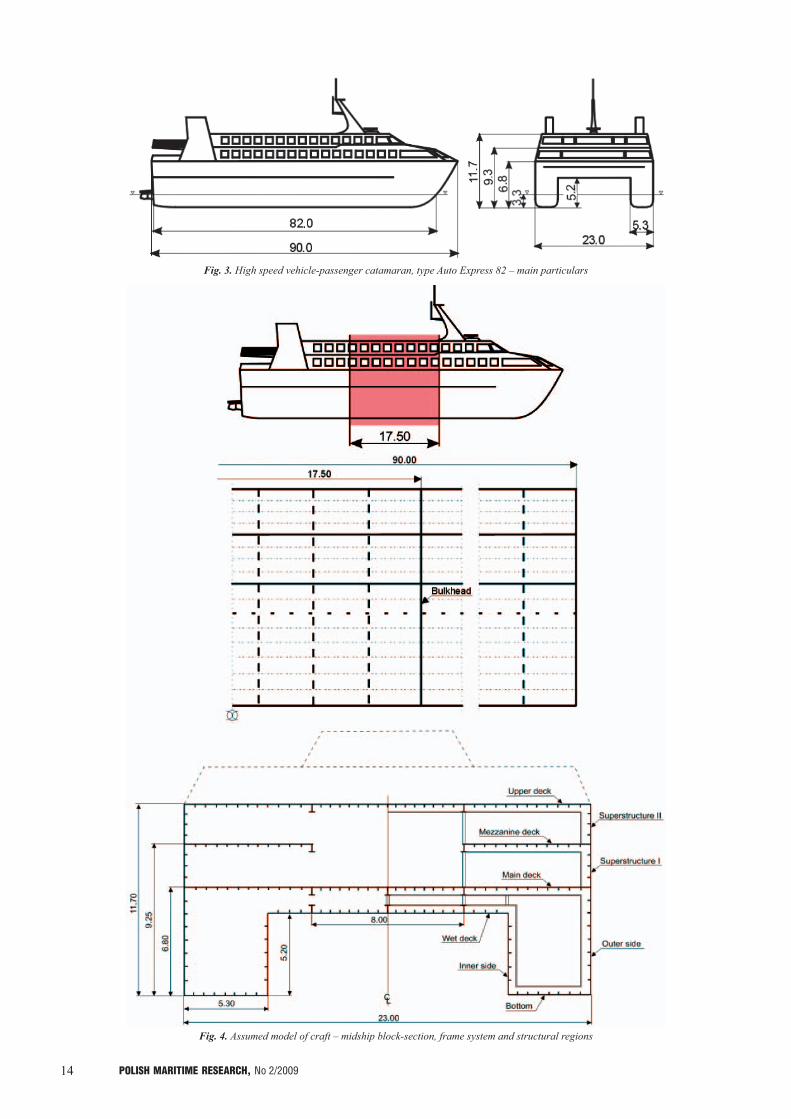
A model based on the Austal Auto Express 82 design developed by Austal [13,32] was applied for the optimization study. The general arrangement of the Austal Auto Express 82 vessel is shown in Fig. 2. Main particulars of the ship are given in Fig. 3. The vessel and his corresponding cross - and longitudinal sections are shown in Fig. 4. For seagoing ships the application domain of initial stage design is clearly the cylindrical and prismatic zone of ship’s central part. For this reason the analysis a midship block-section (17.5 x 23.0 x 11.7 m) was taken. Bulkheads form boundaries of the block in the longitudinal direction. In the block 9 structural regions can be distinguished. The transverse bulkheads were disregarded to minimize the number of design variables.
Fig. 2. High speed vehicle-passenger catamaran, type Austal Auto Express 82 – general arrangement [32]
Fig. 1. Flowchart of computer code for ship structure optimization by genetic algorithm
All regions are longitudinally stiffened with stiffeners; their spacing being different in each structural region. The transverse web frame spacing is common for all the regions. Both types of spacing, stiffener and transverse frame, are considered as design variables.
The structural material is aluminium alloy having properties given in Tab. 1. The 5083-H111 aluminium alloys are used for plates elements while 6082-T6 aluminium alloys are used for bulb extrusions. The plate thicknesses and the bulb and T-bulb extruded stiffener sections are assumed according to the commercial standards and given in Tabs 2-4. Bulb extrusions are used as longitudinal stiffeners while T-bulb extrusions are used as web frames profiles. Practically, the web frames are produced welding the elements cut out of metal sheets. Dimensions of the prefabricated T-bar elements
14 POLISH MARITIME RESEARCH, No 2/2009
Fig. 3. High speed vehicle-passenger catamaran, type Auto Express 82 – main particulars
Fig. 4. Assumed model of craft – midship block-section, frame system and structural regions

15POLISH MARITIME RESEARCH, No 2/2009
are described by four design variables (web height and thickness, and flange breadth and thickness). In the case of extruded bulb a single variable is sufficient to identify the profile, its dimensions and geometric properties. It delimits the computational problem and accelerates analysis. The strength criteria for calculation of plate thicknesses and section moduli of stiffeners and web frames are taken in accordance to the classification rules [36]. It was assumed that bottom, wet deck, outer side and superstructure I and II are subject to pressure of water dependant on the speed and the navigation region. The main deck was loaded by the weight of the trucks transmitted through the tires, mezzanine deck the – weight of the cars while the upper deck – the weight of equipment and passengers. Values of pressure were calculated according to the classification rules.
All genetic parameters are specified by the user before the calculations. This option is very important; the control of the parameter permits to perform search in the direction expected by the designer and in some cases it allows much faster finding solution. The population size, number of variables and number of bits per variable, the total genome length, number of individuals in the population are limited by the available computer memory.
Tab. 1. Properties of structural material – aluminium alloys
No. Property Value
1 Yield stress R0.2125 (for 5083-H111 alloy) [N/mm2]
250 (for 6082-T6 alloy) [N/mm2]
2 Young modulus E 70.000 [N/mm2]
3 Poisson ratio ν 0.33
4 Density ρ 26.1 [kN/m3]
Tab. 2. Thickness of plates
No. Thickness t, [mm] No. Thickness t, [mm]
1 3.00 8 12.00
2 4.00 9 15.00
3 5.00 10 20.00
4 6.00 11 30.00
5 7.00 12 40.00
6 8.00 13 50.00
7 10.00 14 60.00
Tab. 3. Dimensions of bulb extrusions
No. Dimensions (h, b, s, s1)1),
[mm]Cross-sectional area,
[cm2]
1 80 x 19 x 5 x 7.5 5.05
2 100 x 20.5 x 5 x 7.5 6.16
3 120 x 25 x 8 x 12 11.64
4 140 x 27 x 8 x 12 13.64
5 150 x 25 x 6 x 9 10.71
6 160 x 29 x 7 x 10.5 13.51
7 200 x 38 x 10 x 15 24.201) h – cross-section height; b – flange width; s – web thickness; s1 – flange thickness.
A minimum structural weight (volume of structure) was taken as a criterion in the study and was introduced in the definition of the objective function and constraints defined on the base of classification rules. Where structural weight is chosen as the objective function its value depends only on the geometrical properties of the structure (if structural material is fixed). The assumed optimization task is rather simple but the main objective of the study was building and testing the computer code and proving its application for structural topology and sizing optimization of a ship hull.
Tab. 4. Dimensions of T-bulb extrusions
No. Sizes (h, b, s, s1)2),
[mm]Cross-sectional area,
[cm2]1 200 x 100 x 8 x 15 29.80
2 200 x 140 x 8 x 5 35.80
3 200 x 60 x 10 x 12 22.50
4 200 x 50 x 8 x 9.5 21.04
5 210 x 50 x 5 x 16 14.78
6 216 x 140 x 7.6 x 8 37.60
7 220 x 80 x 5 x 8 17.00
8 230 x 80 x 10 x 8 28.60
9 230 x 80 x 5.8 x 8 19.28
10 235 x 170 x 8 x 10 35.00
11 240 x 140 x 6 x 10 27.80
12 260 x 90 x 5 x 9.5 21.08
13 275 x 150 x 9 x 12 41.67
14 280 x 100 x 5 x 8 21.60
15 280 x 100 x 8 x 10 31.60
16 300 x 60 x 15 x 15 51.75
17 310 x 100 x 7 x 16 36.58
18 310 x 123 x 5 x 8 24.94
19 350 x 100 x 8 x 10 37.20
20 350 x 100 x 5 x 8 25.10
21 390 x 150 x 6 x 8 34.92
22 390 x 150 x 6 x 12 40.68
23 400 x 140 x 5 x 8 30.80
24 410 x 100 x 6 x 8 32.12
25 420 x 15 x 5 x 10 35.10
26 420 x 15 x 8 x 10 47.80
27 450 x 100 x 9 x 10 49.60
28 450 x 150 x 10 x 12 61.802) h – cross-section height, b - flange width, s - web thickness, s1 - flange thickness.
FORMULATION OF OPTIMIZATION MODEL
In the most general formulation to solve a ship structural optimization problem means to find a combination of values of the vector of design variables x = col{x1, ..., xi, ..., xn} defining

16 POLISH MARITIME RESEARCH, No 2/2009
the structure which optimizes the objective function f(x). The design variables should also meet complex set of constraints imposed on their values. The constraints formulate the set of admissible solutions. It is assumed that all functions of the optimization problem are real and a number of constraints is finite. Considering computational costs an additional requirement may also be formulated that they should be as small as possible.
As the minimum value of function f is simultaneously the maximum value of –f, therefore the general mathematical formulation of the both optimization problems reads:� find vector of design variables:
x = col{x1, ..., xi, ..., xn}: xi,min ≤ xi ≤ xi,max, i = 1, ..., n
� minimize (maximize):
f(x)� subject:
hk(x) = 0, k = 1, 2, ..., m’gj(x) ≥ 0, j = m’+1, m’+2, ..., m
where:x – a vector of n design variablesf(x) – objective functionhk(x) and gj(x) – constraints.
In the present formulation a set of 37 design variables is applied, cf. Tab. 5 and Fig. 5. Introduction of design variable representing the number of transversal frames in a considered section: x4, and numbers of longitudinal stiffeners in the
regions: x5, x9, x13, x17, x21, x25, x29, x33, x37 enables simultaneous optimization of both topology and scantlings within the presented unified topology - scantling optimization model.
Numbers of stiffeners and transverse web frames, varying throughout the processs of optimization, determine corresponding spacings of them. Scantlings and weights of structural elements: plating, stiffeners and frames are directly dependant on the stiffeners and frames spacings – topological properties of the structure.
Optimizing the structural topology of the ship, a difficult dilemma is to be solved concerning a relation between the number of structural elements in longitudinal and transverse directions and their dimensions, influencing the structural weight. Constraints should also be considered related to the manufacturing process and functional requirements of the ship, e.g. transportation corridors, supporting container seats on the containerships (typically by longitudinal girders and floors in the double bottom) or positioning supports on the girders in the distance enabling entry of cars on ro-ro vessels.
Objective function f(x) for optimization of the hull structure weight is written in the following form:
f(x) = ; r = 9 (2)
where:r – number of structural regionsSWj – structural weight of the j-th structural regionwj – relative weight coefficient (relative importance of
structural weight) of regions varying in the range <0,1>.
The behaviour constraints, ensuring that the designed structure is on the safe side, were formulated for each region
(1)
Fig. 5. Assumed model of craft – specification of design variables

17POLISH MARITIME RESEARCH, No 2/2009
Tab. 5. Simplified specification of bit representation of design variables
No.i
Symbolxi
ItemSubstring
length (no of bits)
Value
Lower limitxi,min
Upper limitxi,max
1 x1 Serial No. of mezzanine deck plate 4 1 10
2 x2 Serial No. of mezzanine deck bulb 3 1 7
3 x3 Serial No. of mezzanine deck t-bulb 4 42 52
4 x4 Number of web frames 3 10 16
5 x5 Number of mezzanine deck stiffeners 4 25 40
6 x6 Serial No. of superstructure i plate 4 1 10
7 x7 Serial No. of superstructure i bulb 3 1 7
8 x8 Serial No. of superstructure i t-bulb 4 42 52
9 x9 Number of superstructure i stiffeners 3 4 11
10 x10 Serial No. of inner side plate 4 1 10
11 x11 Serial No. of inner side bulb 3 1 7
12 x12 Serial No. of inner side t-bulb 4 42 52
13 x13 Number of inner side stiffeners 3 18 25
14 x14 Serial No. of bottom plate 4 1 12
15 x15 Serial No. of bottom bulb 3 1 7
16 x16 Serial No. of bottom t-bulb 4 42 52
17 x17 Number of bottom stiffeners 4 15 25
18 x18 Serial No. of outer side plate 4 1 12
19 x19 Serial No. of outer side bulb 3 1 7
20 x20 Serial No. of outer side t-bulb 4 42 52
21 x21 Number of outer side stiffeners 4 18 33
22 x22 Serial No. of wet deck plate 4 1 12
23 x23 Serial No. of wet deck bulb 3 1 7
24 x24 Serial No. of wet deck t-bulb 4 42 52
25 x25 Number of wet deck stiffeners 4 25 40
26 x26 Serial No. of main deck plate 4 2 12
27 x27 Serial No. of main deck bulb 3 1 7
28 x28 Serial No. of main deck t-bulb 4 42 52
29 x29 Number of main deck stiffeners 4 25 40
30 x30 Serial No. of superstructure ii plate 4 1 10
31 x31 Serial No. of superstructure ii bulb 3 1 7
32 x32 Serial No. of superstructure ii t-bulb 4 42 52
33 x33 Number of superstructure ii stiffeners 3 4 11
34 x34 Serial No. of upper deck plate 4 1 10
35 x35 Serial No. of upper deck bulb 3 1 7
36 x36 Serial No. of upper deck t-bulb 4 42 52
37 x37 Number of upper deck stiffeners 4 25 40
Multivariable string length (chromosome length) 135

18 POLISH MARITIME RESEARCH, No 2/2009
according to the classification rules [36] constitute a part of the set of inequality constraints gj(x):� required plate thickness tj,rule based on the permissible
bending stress:
tj – tj,rule ≥ 0 (3)
where:tj – actual value of plate thickness in j-th region
� required section moduli of stiffeners Zs,j,rule:
Zs,j – Zs,j,rule ≥ 0 (4)
where:Zs,j – actual value of the section modulus of stiffeners in
j-th region
� required section moduli of web frames Zf,j,rule:
Zf,j – Zf,rule ≥ 0 (5)
where:Zf,j – actual value of the section modulus of web frames
in j-th region
� required shear area of stiffeners At,s,j,rule:
At,s,j – At,s,j,rule ≥ 0 (6)
where:At,s,j – actual value of shear area of stiffeners in j-th
region
� required shear area of web frames At,f,j,rule:
At,f,j – At,f,j,rule ≥ 0 (7)
where:At,f,j – actual value of the shear area of web frames in j-th
region.
Side constraints hk(x), mathematically defined as equalibrum constraints, for design variables are given in Tab. 5. They correspond to the limitations of the range of the profile set. Some of them are pointed according to the author’ experience in improving the calculation convergence.
The additional geometrical constraints were introduced due to “good practice” rules:� assumed relation between the plate thickness and web frame
thickness:
tj - tf,w,j ≥ 0 (8)
where:tj – actual value of the plate thickness in j-th regiontf,w,j – actual value of web frame thickness in j-th region
� assumed relation between the plate thickness and stiffener web thickness:
tj – ts,w,j ≥ 0 (9)
where:tj – actual value of the plate thickness in j-th regionts,w,j – actual value of stiffener web thickness in j-th
region
� assumed minimal distance between the edges of frame flanges:
l(x4+1) - bf,j ≥ 0.3 m (10)
where:bf,j – actual value of frame flange breadth in j-th region.
These relationships supplement the set of inequality constraints gj(x).
Finally, taking into consideration all specified assumptions, the optimization model can be written as follows:� find vector of design variables x = col{x1, ..., xi, ..., xn},
xi, i = 1, ..., 37 as shown in Tab. 5� minimise objective function f(x) given by Eq. (2)� subject to behavior constraints given by Eqs. (3) ÷ (7), side
constraints given in Tab. 5 and geometrical constraints given by Eqs. (8) ÷ (10) build a set of equality hj(x) and inequality gj(x) constraints.
DESCRIPTION OF THE GENETIC MODEL
General
The topology and sizing optimization problem described in Sections 4 and 5 contains a large number of discrete design variables and also a large number of constraints. In such a case GA seems to be especially useful. Solution of the optimization problem by GA calls for formulation of an appropriate optimization model. The model described in Sections 4 and 5 was reformulated into an optimization model according to requirements of the GA and that model was further used to develop suitable procedures and define search parameters to be used in the computer code.
The genetic type model should cover:� definition of chromosome structure� definition of fitness function� definition of genetic operators suitable for the defined
chromosome structures and optimization task� list of the searching control parameters.
Chromosome structure
The space of possible solutions is a space of structural variants of the assumed model. The hull structural model is identified by the vector x of 37 design variables, xi. Each variable is represented by a string of bits used as chromosome substring in GA. The simple binary code was applied. In Tab. 5a simplified specification for bit representation of all design variables is shown. Such coding implies that each variant of solution is represented by a bit string named chromosome. Length of chromosome which represents of structural variant is equal to the sum of all substrings. Number of possible solutions equals the product of values of all variables. In the present work the chromosome length is equal to 135 bits making the number of possible solutions approximately equal to 1038.
Fitness function
A fitness function is used to determine how the ship structure topology and sizing is suitable for a given condition in the optimum design with a GA. The design problem defined in previous parts of this paper is to find the minimum weight of a hull structure without violating the constraints. In order to transform the constrained problem into unconstrained one and due to the fact that GA does not depend on continuity and existence of the derivatives, so called “penalty method” have been used. The contribution of the penalty terms is proportional to violation of the constraint. In the method the augmented objective function of unconstrained minimisation problem is expressed as:
Φ(x) = f(x) – (11)
where:Φ(x) – augmented objective function of unconstrained
minimisation

19POLISH MARITIME RESEARCH, No 2/2009
f(x) – objective function given by Eq. (2)Pk – penalty term to violation of the k-th constraintwk – weight coefficients for penalty termsnc – number of constraints.
Weight coefficients wk are adjusted by trial.
Additionally a simple transformation of minimisation problem (in which the objective function is formulated for the minimisation) into the maximization is necessary for the GA procedures (searching of the best individuals). It can be done multiplying the objective function by (-1). In that way, the minimization of the augmented objective function was transformed into a maximisation search using:
Fj = Φmax - Φj(x) (12)
where:Fj – fitness function for j-th solutionΦj(x) – augmented objective function for j-th solutionΦmax – maximum value of the augmented function from all
solutions in the simulation.
The value of parameter Φmax has to be arbitrary chosen by a user of the software to avoid negative fitness values. Its value should be greater than the expected largest value of Φj(x) in the simulation. In the presented approach the value Φmax = 100,000 was assumed.
Genetic operators
The basic genetic algorithm (Simple Genetic Algorithm - SGA) produces variants of the new population using the three main operators that constitute the GA search mechanism: selection, mutation and crossover. The algorithm in present work was extended by introduction of elitism and updating.
Many authors described the selection operators which are responsible on chromosome selection due to their fitness function value [1, 7, 11, 21]. After the analysis of the selection operators a roulette concept was applied for proportional selection. The roulette wheel selection is a process in which individual chromosomes (strings) are chosen according to their fitness function values; it means that strings with higher fitness value have higher probability of reproducing new strings in the next generation. In this selection strategy the greater fitness function value makes the individuals more important in a process of population growth and causes transmittion of their genes to the next generations.
The mutation operator which introduces a random changes of the chromosome was also described [1,21]. Mutation is a random modification of the chromosome. It gives new information to the population and adds diversity to the mate pool (pool of parents selected for reproduction). Without the mutation, it is hard to reach to solution point that is located far from the current direction of search, while due to introduction of the random mutation operator the probability of reaching any point in the search space never equals zero. This operator also prevents against to the premature convergence of GA to one of the local optima solutions, thus supporting exploration of the global search space.
The crossover operator combines the features of two parent chromosomes to create new solutions. The crossover allows to explore a local area in the solution space. Analysis of the features of the described operators [1, 11, 21] led to elaboration of own, n-point, random crossover operator. The crossover parameters in this case are: the lowest n_x_site_min and the greatest n_x_site_max number of the crossover points and the crossover probability pc. The operator works automatically and
independently for each pair being intersected (with probability pc), and it sets the number of crossover points n_x_site. The number of points is a random variable inside the set range [n_x_site_min, n_x_site_max]. The test calculations proved high effectiveness and quicker convergence of the algorithm in comparison to algorithm realizing single-point crossover. Concurrently, it was found that the number of crossover points n_x_site_max greater than 7 did not improve convergence of the algorithm. Therefore, the lowest and greatest values of the crossover points were set as following: n_x_site_min = 1, n_x_site_max = 7 (Tab. 6).
The effectiveness of the algorithm was improved with application of an additional updating operator as well as introduction of elitist strategy.
Tab. 6. Genetic model and values of control parameters
No. Symbol Description Value
1 ng Number of generations 5,000
2 ni Size of population 2,000
3 np Number of pretenders 3
4 pm Mutation probability 0.066
5 pc Crossover probability 0.80
6 c_strategyDenotation of crossover strategy
(0 for fixed, 1 for random number of crossover points)
1
7 n_x_site_min The lowest number of crossover points 1
8 n_x_site_max The greatest number of crossover points 7
9 pu Update probability 0.33
10 elitism
Logical variable to switch on (elitism = yes) and off
(elitism = no) the pretender selection strategy
yes
Random character of selection, mutation and crossing operators can have an effect that these are not the best fitting variants of the parental population which will be selected for crossing. Even in the case they will be selected, the result will be that progeny may have less adaptation level. Thus the efficient genome can be lost. Elitist strategy mitigates the potential effects of loss of genetic material copying certain number of best adapted parental individuals to progeny generation. In the most cases the elitist strategy increases the rate of dominating population by well-adapted individuals, accelerating the convergence of the algorithm. The algorithm selects fixed number of parental individuals np having the greatest values of the fitness function and the same number of descendant individuals having the least values of the fitness. Selected descendants are substituted by selected parents. In this way the operator increases exploitation the of searching space. The number of pretenders np is given in Tab. 6. Update operator with fixed probability of updating pu introduces an individual, randomly selected from the parental population, to the progeny population, replacing a descendant less adapted individual. The value of probability of updating pu is also given in Tab. 6. This operator enhances exploration of searching space at the cost of decreasing the search convergence. It also prevents the algorithm from converging to a local minimum. Both operators acts in opposite directions, and they should be well balanced: exploitation of attractive areas found in the

20 POLISH MARITIME RESEARCH, No 2/2009
searching spaces as well as exploration of searching space to find another attractive areas in the searching space depends on the user’s experience.
Control parameters
Single program run with the defined genetic model is characterized by values of ten control parameters (Tab. 6).
For selection of more control parameters it is not possible to formulate quantitative premises because of the lack of an appropriate mathematical model for analysis of GA convergency in relation to control parameters. The control parameters were set due to test calculations results to achieve a required algorithm convergence; their values are presented in Tab. 6.
Conclusion
Finally, taking into consideration all specified assumptions, the genetic model can be written as follows:� chromosome structure specified in Tab. 5� fitness function given by Eq. 12� genetic operators described in subsection 6.4� control parameters specified and described in subsection
6.5 and specified in Tab. 6.
OPTIMIZATION CALCULATIONS
To verify the correctness of the optimization procedure several test cases have been carried out using the model described in Sections 4-6. Each experiment is characterised by the 10 parameters, given in Tab. 6, controling the search process. The set of experiment parameters are as follows: (ng, ni, np, pm, pc, c_strategy, n_x_site_min, n_x_site_max, pu, elitism) = (5,000, 2,000, 3, 0.066, 0.8, 1, 1, 7, 0.033, true). A total number of 106 individuals were tested in the whole simulation. Results of typical search trial are presented in Tab. 7-8 and Fig. 6.
The lowest value of the objective function, f(x) = 4.817,35 kN, was found in the 868th generation. The corresponding values of design variables are given in Tab. 7.
All values of the hull structural weight for feasible individuals searched in the simulation are presented in Fig. 7. The solid line represents the front of optimal solutions. It is composed of minimal (optimal) values of the structural weight received in the following simulation. All variants situated above the front of optimal solutions line are feasible but structural weight of these wariants is greater than those situated on the front line. It can be seen how difficult it is to find the global optimum in the space search. Most of admissible variants created and evaluated during the simulation are remote from the global optimum and were used for the exploration of search space. A significant part of the computational effort is thus used by the algorithm for the exploration of search space and only a small part for exploitation of local optima. Such a ”computational extravagance” is typical for all optimization algorithms employing random processes.
Fig. 7. Evolution of structural weight values over 5.000 generations; solid line for absolutely minimal structural weight found during
simulation (only feasible solutions are shown)
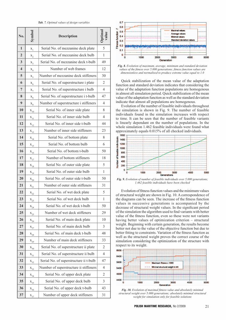
The graphs of the maximum, average, minimum and variance values of fitness across 5.000 generations for simulation are presented in Fig. 8. The saturation was nearly achieved in this simulation. The maximum normalised fitness value is nearly 0,645. The standard deviation value is approximately constant and equal to 0,075 for all generations what means that heredity of generations is approximately constant over simulation. Variation of macroscopic quantities forming subsequential populations created throughout the simulation indicates evolutionally correct computations and that, for assumed values of the control parameters, it was not necessary to continue the simulation beyond assumed value of 5.000 generations.
Fig. 6. Optimal dimensions and scantlings of vessel structure
21POLISH MARITIME RESEARCH, No 2/2009
Fig. 8. Evolution of maximum, average, minimum and standard deviation values of the fitness over 5.000 generations; fitness function values are dimensionless and normalised to produce extreme value equal to 1.0
Quick stabilization of the mean value of the adaptation function and standard deviation indicates that considering the value of the adaptation function populations are homogenous in almost all simulation period. Quick stabilization of the mean value of the adaptation function as well as the standard deviation indicate that almost all populations are homogenous.
Evolution of the number of feasible individuals throughout the simulation is shown in Fig. 9. The number of feasible individuals found in the simulation increases with respect to time. It can be seen that the number of feasible variants is linearly dependant on the number of populations. In the whole simulation 1.462 feasible individuals were found what approximately equals 0.015% of all checked individuals.
Fig. 9. Evolution of number of feasible individuals over 5.000 generations; 1.462 feasible individuals have been checked
Evolution of fitness function values and the minimum values of structural weight are shown in Fig. 10. A correspondence of the diagrams can be seen. The increase of the fitness function values in successive generations is accompanied by the decrease of structural weight values. In the significant period of the simulation the algorithm used to find variants with better value of the fitness function, even so these were not variants having better values of optimization criterion – structural weight. Beginning with certain generation, the results become better not due to the value of the objective function but due to better fitting to constraints. Variation of the fitness function as well as the structural weight proves the correct course of the simulation considering the optimization of the structure with respect to its weight.
Fig. 10. Evolution of maximal fitness value and absolutely minimal structural weight over 5.000 generations; absolutely minimal structural
weight for simulation only for feasible solutions
Tab. 7. Optimal values of design variables
No.Sy
mbo
lDescription
Opt
imal
va
lue
1 x1 Serial No. of mezzanine deck plate 5
2 x2 Serial No. of mezzanine deck bulb 1
3 x3 Serial No. of mezzanine deck t-bulb 49
4 x4 Number of web frames 12
5 x5 Number of mezzanine deck stiffeners 30
6 x6 Serial No. of superstructure i plate 2
7 x7 Serial No. of superstructure i bulb 4
8 x8 Serial No. of superstructure i t-bulb 47
9 x9 Number of superstructure i stiffeners 4
10 x10 Serial No. of inner side plate 8
11 x11 Serial No. of inner side bulb 4
12 x12 Serial No. of inner side t-bulb 44
13 x13 Number of inner side stiffeners 23
14 x14 Serial No. of bottom plate 8
15 x15 Serial No. of bottom bulb 6
16 x16 Serial No. of bottom t-bulb 50
17 x17 Number of bottom stiffeners 18
18 x18 Serial No. of outer side plate 5
19 x19 Serial No. of outer side bulb 1
20 x20 Serial No. of outer side t-bulb 50
21 x21 Number of outer side stiffeners 31
22 x22 Serial No. of wet deck plate 5
23 x23 Serial No. of wet deck bulb 1
24 x24 Serial No. of wet deck t-bulb 50
25 x25 Number of wet deck stiffeners 29
26 x26 Serial No. of main deck plate 10
27 x27 Serial No. of main deck bulb 3
28 x28 Serial No. of main deck t-bulb 48
29 x29 Number of main deck stiffeners 33
30 x30 Serial No. of superstructure ii plate 2
31 x31 Serial No. of superstructure ii bulb 4
32 x32 Serial No. of superstructure ii t-bulb 47
33 x33 Number of superstructure ii stiffeners 4
34 x34 Serial No. of upper deck plate 2
35 x35 Serial No. of upper deck bulb 3
36 x36 Serial No. of upper deck t-bulb 43
37 x37 Number of upper deck stiffeners 31

22 POLISH MARITIME RESEARCH, No 2/2009
Both figures, Fig. 9 and 10, indicate quantitatively that the computer simulation realizing evolutional searching for the solution of the topology-sizing in relation to weight of the ship structure optimization was successful and the final result can be taken as the solution of the formulated optimization problem. As it is known, the conclusion cannot be confirmed by precise mathematical methods.
Number of all possible variants in the genetic model, number of checked individuals over 5.000 generations and number of feasible individuals checked over simulation are shown in Fig. 11. Presented values show how much computational effort is used to find a small number of the feasible variants among which we expect the optimum variant be located. It seems that it is a cost we should accept if we want to keep the high ability of the algorithm to explore of the solution space. Retaining the values of another control parameters, the number of the feasible variants can be increased adjusting variation ranges of the design variables. The ranges can be either narrowed or shifted towards larger values of the design variables so that it is easier to obtain feasible variants. In each specific case the selection of the strategy is dependant on the user:• whether to allow the wider searching solution space
expecting solutions closer to optimum can be found at the expense of longer computational time,
• or to decrease the computational time accepting that the solutions will be more remote from the optimum.
Fig. 11. 1. number of all possible individuals (1039 individuals), 2. number of checked variants (107 variants), 3. number of feasible
variants checked over simulation (1462 variants); area is proportional to logarithm of number of variants
Methodology of scientific investigation requires that the quantitative results be verified. In this case the verification can be performed either (i) comparing to appropriate values of a real structure or (ii) comparing to the recognized results of comparable computations performed by other authors. Concerning (i) the author does not have corresponding data since the shipyards usually do not publish the data on structural weight. Concerning (ii) it should be remarked that similar optimization problems referring to ship structures are rarely undertaken by the other authors therefore the examples are unique or unpublished. Specifically, the author does not have a reference data on the structural model taken for the investigation. In this context the presented investigation does not answer the question whether the obtained results indicate a possibility to design the structure lighter than actual but the existence of a method which is applicable for solution of the unified topology - size optimization for a sea-going ship structure in more general sense.
The investigation carried out within the present paper confirmed the three unquestionable advantages of GA which make them attractive and useful for optimization of ship structures: (i) resistance to existence of many local extremes in the search space, (ii) lack of necessity of differentiation of the objective and limit functions and (iii) easiness of modeling and solution of the problems involving discrete variables. Of course they also have disadvantages, the most important being:
(i) computational extravagance (large computational cost used for exploration of the search space) and (ii) lack of formal convergence criteria. Additional advantages which can decide perspectively on the more common use of the algorithms are: (i) existence of developed and published algorithms of multi-criteria optimization as well as (ii) effective computations on networks of computers or muti-processor computers.
Significant computational costs required for ship structural optimization employing GA cause, at the present speed of commercial computer systems, strong doubts on possibility of application of direct methods of structural analysis for estimation of behaviour constraints. It seems that direct application e.g. regularly used in practice the finite element method for the analysis of millions or even billions variants checked in the exploration of decision space seems impossible. Especially in the preliminary designing where many optimization investigations are to be performed in short time. In such a situation methods can be searched to limit the number of such calculations to e.g. preselected variants. A hybrid system can also be proposed where e.g. GA will allow to create, using fast rule equations or simplified methods of analysis, a set of variants localized in the vicinity of extremum and then searching the optimum solution using the selected analytical method using the direct methods of structural analysis.
CONCLUSIONS
� The application of the genetic algorithm concept to solve the practical design problem of the optimization of hull structures of high speed craft was presented. The problem of weight minimisation for a three dimensional full midship block-section of the high speed catamaran hull was described.
� In the study the design problem was limited to the minimisation of the hull structural weight but it can be easily extended to include other criteria such as production cost what will be a subject of the further studies.
� It was proven in the study that the GA allows to include in the optimization model a large number of design variables of the real ship structure. Introducing constraints related to strength, fabrication and standardisation is not difficult and may cover a more representative set of criteria.
� Simultaneous optimization of topology and scantlings is possible using the present approach. Enhancement of the sizing optimization (the standard task of the structural optimization) to allow for the topology optimization requires disproportional computational effort. It is an effect of both increase of the search space by introducing design variables referring to the structural topology as well as increase of number of generations and number of individuals to ensure satisfactory convergence of the optimization process.
� Additionally the GA realisation described in the paper is also under continuous development directed towards implementation of other genetic operators, genetic encoding, multi-objective optimization etc. as well as including some other constraints.
� Practical application of the GA to ship structural optimization calls for significant limitation of an optimization problem in the way of spatial delimitation of the structural region subject to optimization and/or limitation of variation of design variables.

23POLISH MARITIME RESEARCH, No 2/2009
� As the final conclusion it can be said that the study confirmed that proposed realisation of the GA presented a potentially powerful tool for optimising of the topology and sizing of ship hull structures.
� The present paper is a successful attempt of unification of problems of topology and sizing optimization of ship structure and their solution using the GA. It was proven that the GA can be considered as a good method for solution of more general unified shape-material-topology-sizing optimization problems.
BIBLIOGRAPHY
1. Back T.: Evolutionary Algorithms in Theory and Practice. Oxford University Press, New York, 1996
2. Bendsoe M.P., Kikuchi N.: Generating Optimal Topologies in Structural Design Using a Homogenization Method. Computer Methods in Applied Mechanics and Engineering 1988
3. Coley D.A.: An Introduction to Genetic Algorithms for Scientists and Engineers. World Scientific, Singapore, 1999
4. Carroll D.L.: Genetic Algorithms and Optimizing Chemical Oxygen-iodine Lasers. In: Developments in Theoretical and Applied Mechanics, Vol. XVIII. School of Engineering, The University of Alabama, 1996
5. Davis L.: Handbook of Genetic Algorithms. New York:Van Nostrand, 1991
6. De Jong K.A.: An analysis of the behavior of a class of genetic adaptive systems. Ph.D. Thesis, University of Michigan, 1975
7. De Jong K.: On Decentralizing Selection Algorithms. In: Proceedings of the Sixth International Conference on Genetic Algorithms. Morgan Kaufmann Publishers, San Francisco, 1995
8. Fast Ferry International Star Cruises introduces Auto Express 82 catamaran. 1998
9. Fleury C.: Mathematical programming methods for constrained optimization: Dual Methods. Structural optimization: Status and Promise, Progress in Astronautics and Aeronautics 1993
10. Goldberg D.E.: Genetic Algorithms in Search, Optimization, and Machine Learning. Addison-Wesley Publishing Company, Inc., 1989
11. Goldberg D.E., Deb K.: A Comparative Analysis of Selection Schemes Used in Genetic Algorithms. In: Foundations of Genetic Algorithms. Morgan Kaufmann Publishers, San Mateo, 1991
12. Goldberg D.E., Deb K., Clark J.H.: Genetic Algorithms, Noise, and Sizing of Populations. Complex Systems 1992
13. HANSA Polish fast ferry “Boomerang”. 199714. Holland J.H.: Adaptation in Natural and Artificial Systems. The
University of Michigan Press, Ann Arbor, 197515. Hughes O.F., Mistree F., Zanic V.: A Practical Method for the
Rational Design of Ship Structures. Journal of Ship Research 1980
16. Hughes O.F.: Ship Structural Design: A Rationally-Based, Computer-Aided Optimization Approach. SNAME, New Jersey, 1988
17. Jang C.D., Seo S.I.: A study on the Optimum Structural Design of Surface Effect Ships. Marine Structures 1996; 9:519-544
18. Krol W.: Midship section design using a bilevel production cost optimization scheme. Journal of Ship Production 1991
19. Lund S.: Tanker Frame Optimisation by Means of SUMT-Transformation and Behaviour Models. Norges Tekniske Høgskole, Trondheim, 1970
20. Man K.F. Tang K.S, Kwong S.: Genetic Algorithms. Springer-Verlag, London, 1999
21. Michalewicz Z.: Genetic Algorithms + Data Structures = Evolution Programs. Springer-Berlin-Heidelberg: Springer-Verlag, 1996
22. Moe J., Lund S.: Cost and weight minimization of structures with special emphasis on longitudinal strength members of tankers. Transactions RINA 1968
23. Nobukawa H., Zhou G.: Discrete optimization of ship structures with genetic algorithm. Journal of The Society of Naval Architects of Japan 1996
24. Nobukawa H., Kitamura M., Yang F., Zhou G.: Optimization of Engine Room Structure under Static and Dynamic Constraints Using Genetic Algorithms. Journal of The Society of Naval Architects of Japan 1998
25. Okada T., Neki I.: Utilization of genetic algorithm for optimizing the design of ship hull structures. Journal of The Society of Naval Architects of Japan 1992
26. Rachman M., Caldwell J.: Ship structures: Improvement by rational design optimisation. International Shipbuilding Progress 1995
27. Rigo Ph.: Least-Cost Structural Optimization Oriented Preliminary Design. Journal of Ship Production 2001
28. Rigo Ph.: A module-oriented tool for optimum design of stiffened structures – Part I. Marine Structures 2001
29. Sekulski Z., Jastrzebski T.: 3D optimisation problem of the ship hull structure by the Genetic Algorithm. Marine Technology Transactions 1999
30. Sen P., Shi W., Caldwell J.: Efficient design of panel structures by a general multiple criteria utility. Engineering Optimization 1989
31. Sen P., Shi W., Caldwell J.: Guru: A generalised multi-criteria utility for reanalysis in design. Engineering Optimization 1989
32. Significant Ships Boomerang: catamaran ferry for Baltic Service 1997
33. Spears W.M., De Jong K.A.: An Analysis of Multi-Point Crossover. Foundations of Genetic Algorithms. Morgan Kaufmann Publishers, San Mateo, 1991
34. Stoffa P.L., Sen M.K.: Nonlinear multiparameter optimization using genetic algorithms: Inversion of plane-wave seismograms. Geophysics 1989
35. Syswerda G.: Uniform Crossover in Genetic Algorithms. Proceedings of the Third International Conference on Genetic Algorithms. Morgan Kaufmann Publishers, 1989
36. UNITAS Rules for the Construction and Classification of High Speed Craft. 1995
37. Zhou G., Nobukawa H., Yang F.: Discrete optimization of cargo ship with large hatch opening by genetic algorithms. ICCAS’97, Proceedings of the 9th International Conference on Computer Applications in Shipbuilding. Yokohama, Japan, 1997
38. Zanic V., Jancijev T., Aandrie J.: Mathematical models for analysis and optimization in concept and preliminary ship structural design. Congress of International Maritime Association of the Mediterranean (IMAM’ 2000). Italy, 2000.
CONTACT WITH THE AUTHORZbigniew Sekulski, Ph. D.
West Pomeranian University of Technology, SzczecinFaculty of Marine Technology
AL. Piastów 4171-065 Szczecin, POLAND
e-mail: [email protected]
24 POLISH MARITIME RESEARCH, No 2/2009
INTRODUCTION
There is an increasing demand to facilitate the use of marine environment by planning onshore infrastructures, offshore platforms, high speed vessels, etc., which are all along with high costs in design as well as in construction. Computational Fluid Dynamics (CFD) shortens the way to meet many design requirements in hydrodynamics. Here, a unified algorithm is developed and examined to tackle hydrodynamic problems including fluid-structure interaction with characteristics indicated in Tab. 1.
However, one encounters three major difficulties to make decision about them in a numerical algorithm to solve such problems. They are presented in the first row of Tab. 2. Available approaches and selected methods based on covered hydrodynamics problems specifications (Tab. 1) are also summarized in second and third row of this Table.
Governing equations are reviewed in section 2. They have to be revised according to requirements in simulation of two-phase flow using FV discretisation in moving meshes. Section 3 is dedicated to discretisation. Solution of the Navier-Stokes equations is discussed in section 4. Section 5 is devoted to overlapping mesh motion modeling strategy. A general algorithm to concisely show the relation between different parts of developed fluid-structure interaction solver is presented in section 6. The present procedure is coded and verified in section 7 by applying it to some flows for which either numerical solution or experimental data are available.
Application of Overlapping Mesh in Numerical Hydrodynamics
Roozbeh Panahi, Assoc. Prof.Mehdi Shafieefar, Assoc. Prof.Tarbiat Modares University
ABSTRACT
A Finite Volume (FV) algorithm is presented to investigate two-dimensional hydrodynamic problems including viscous free surface flow interaction with free rigid bodies in the case of large and/or relative motions. Two-phase flow with complex deformations at the interface is simulated using a fractional step-volume of fluid algorithm while it is also capable of representing a high quality wave tank, according to implemented temporal discretisation. Rigid body motions are also captured using two overset meshes. Flow variables are transferred using a simple fully implicit non-conservative interpolation scheme which maintains the second-order accuracy of implemented spatial discretisation. A code is developed and an appropriate set of problems are investigated. Results show a good potential to develop a virtual
hydrodynamics laboratory.
Keywords: finite volume; two-phase flow; overlapping mesh; fluid-structure interaction
Tab. 1. Scope of encountered problems including fluid-structure interaction in the context of an interfacial flow
Fluid and Flow Structure and Motion
without surface tension 2D
with homogenous property distribution fixed/free(3-DoF)
without suspended particles floating/submerged
Incompressible large amplitude motions
Viscous Rigid
Rotational with relative motions
Newtonian with auxiliary equipments(propeller, rudder, mooring
line, ...)steady/unsteady
Laminar with geometrical complexity
one/two-phase
with large interface deformations
Potentials of the algorithm are demonstrated where complex interfacial flow, relative and/or large amplitude motions as well as wave generation and propagation are of interest.
POLISH MARITIME RESEARCH 2(60) 2009 Vol 16; pp. 24-3310.2478/v10012-008-0018-4

25POLISH MARITIME RESEARCH, No 2/2009
GOVERNING EQUATIONS
According to characteristics of the encountered two-phase flow field, see Tab. 1, and implemented motion modeling strategy, the following set of equations in the Arbitrary Lagrangian-Eulerian (ALE) Cartesian form are used:
(1)
(2)
(3)
where:ρeff = αρ1 + (1 – α)ρ2 and νeff = αν1 + (1 – α)ν2 are density and dynamic viscosity of an effective phase as a combination of phases volume fraction α. It is obvious that α is calculated in each Control Volume (CV) by solving a transport equation. Volume fraction of zero in a CV indicates the presence of one fluid and the unity indicates the other fluid; urel = u – um is the fluid velocity vector u relative to the mesh velocity vector um and n represents a unit vector normal to a CV face. ui is the velocity component in the i Cartesian direction, P stands for the pressure, ni is the i Cartesian direction component of n and gi indicates the gravity component in this direction.
Movements of a free rigid body are also included in this study. They are calculated based on loads acting on the body, by solving the linear and angular momentum equations. Such loads can be raised from effects of flow field, body weight and probably external components. Rigid body motion equations are treated in a Global Coordinate System (GCS); a non-rotating, non-accelerating Newtonian reference system.
DISCRETISATION
Here, discretisation of all differential governing equations is reviewed. More details can be found in a recent paper of the authors (Jahanbakhsh et al., 2007).
Momentum Conservation Equations
On the l.h.s of Eq.(2), the simplest approximation for the spatial discretisation of the first term (unsteady term) is to replace it by the product of the value of the integrand at the CV
center and the volume of the CV. Convection term (the second term) is also discretised using Gamma interpolation (Jasak, 1996). Besides, on the r.h.s. of Eq.(2), using the common Linear Interpolations (LI) to discretise pressure term (the first term) results in oscillations in the velocity field in the case of two-phase flow. Such oscillations lead the solution to a divergence, especially when there are two phases with a high density ratio e.g. water and air. Here, a Piecewise LI (PLI) is implemented, recently introduced by the authors (Jahanbakhsh et al., 2007). The second term (diffusion term) is treated by over-relaxed interpolation (Jasak, 1996). Finally, the last term (gravity term) is discretised as the unsteady term.
Temporal discretisation of the momentum conservation equations is in direct relation to the way that the pressure and the velocity fields are coupled. So, it is discussed together with implemented fractional step method in the next section.
Volume Fraction Transport Equation
Spatial discretisation of the unsteady term is done similar to that of the momentum conservation equations. About its temporal discretisation, although the first-order Euler implicit interpolation is the obvious choice but it has been shown in the numerical results that such a temporal discretisation is not a good option when wave generation and propagation are the case. In contrast, the second-order three-time-levels temporal discretisation proposes a minimum level of diffusion in such problems. The Compressive Interface Capturing Scheme for Arbitrary Meshes (CICSAM) (Ubbink and Issa, 1999) is used for spatial discretisation of the convection term as well as Crank-Nicholson interpolation for its temporal discretisation according to an investigation conducted by the authors (Panahi et al., 2005).
COUPLING OF THE PRESSURE AND THE VELOCITY FIELDS
To compute the pressure and the velocity fields, the fractional step method of Kim and Choi (Kim and Choi, 2000) is implemented. Here, Crank-Nicholson scheme is used for the temporal discretisation of the convection term in contrast to Adams-bashforth scheme used in the original method. In addition, convection term is linearized using Picard iteration method instead of the Newton’s method in (Kim and Choi, 2000). Such an algorithm can be found as a flowchart in (Panahi et al., 2006a).
OVERLAPPING MESH
As mentioned earlier, to simulate fluid-structure interaction including moving bodies, a motion modeling strategy is
Tab. 2. Encountered problems, available approaches and implemented methods
Case Available approaches Implemented approachCoupling of the pressure and the
velocity fields(Ferziger and peric, 2002)
Predictor-correctorArtificial compressibility
Fractional stepFractional step
Simulation of free surface (Ubbink and issa, 1999)
Surface trackingSurface capturing Surface capturing
Capturing of rigid body motions in a domain
Body-attached/moving mesh (panahi et al., 2006A)Deformable mesh (chentanez et al., 2006)
Re-mesh (tremel et al., 2007)Sliding mesh (blades and marcum, 2007)Overlapping mesh (carrica et al., 2007)
Cartesian mesh (mittal and iccarino, 2005)
Overlapping mesh
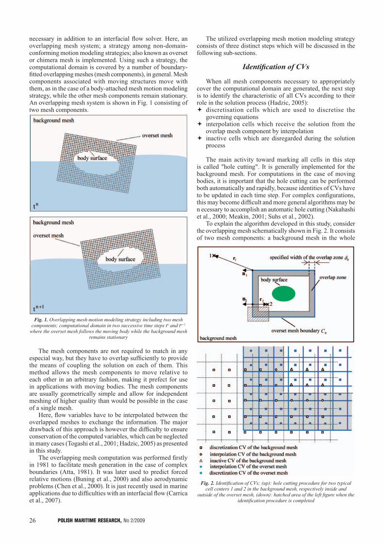
26 POLISH MARITIME RESEARCH, No 2/2009
necessary in addition to an interfacial flow solver. Here, an overlapping mesh system; a strategy among non-domain-conforming motion modeling strategies; also known as overset or chimera mesh is implemented. Using such a strategy, the computational domain is covered by a number of boundary-fitted overlapping meshes (mesh components), in general. Mesh components associated with moving structures move with them, as in the case of a body-attached mesh motion modeling strategy, while the other mesh components remain stationary. An overlapping mesh system is shown in Fig. 1 consisting of two mesh components.
Fig. 1. Overlapping mesh motion modeling strategy including two mesh components; computational domain in two successive time steps tn and tn+1
where the overset mesh follows the moving body while the background mesh remains stationary
The mesh components are not required to match in any especial way, but they have to overlap sufficiently to provide the means of coupling the solution on each of them. This method allows the mesh components to move relative to each other in an arbitrary fashion, making it prefect for use in applications with moving bodies. The mesh components are usually geometrically simple and allow for independent meshing of higher quality than would be possible in the case of a single mesh.
Here, flow variables have to be interpolated between the overlapped meshes to exchange the information. The major drawback of this approach is however the difficulty to ensure conservation of the computed variables, which can be neglected in many cases (Togashi et al., 2001; Hadzic, 2005) as presented in this study.
The overlapping mesh computation was performed firstly in 1981 to facilitate mesh generation in the case of complex boundaries (Atta, 1981). It was later used to predict forced relative motions (Buning et al., 2000) and also aerodynamic problems (Chen et al., 2000). It is just recently used in marine applications due to difficulties with an interfacial flow (Carrica et al., 2007).
The utilized overlapping mesh motion modeling strategy consists of three distinct steps which will be discussed in the following sub-sections.
Identification of CVs
When all mesh components necessary to appropriately cover the computational domain are generated, the next step is to identify the characteristic of all CVs according to their role in the solution process (Hadzic, 2005):� discretisation cells which are used to discretise the
governing equations� interpolation cells which receive the solution from the
overlap mesh component by interpolation� inactive cells which are disregarded during the solution
process
The main activity toward marking all cells in this step is called "hole cutting". It is generally implemented for the background mesh. For computations in the case of moving bodies, it is important that the hole cutting can be performed both automatically and rapidly, because identities of CVs have to be updated in each time step. For complex configurations, this may become difficult and more general algorithms may be n ecessary to accomplish an automatic hole cutting (Nakahashi et al., 2000; Meakin, 2001; Suhs et al., 2002).
To explain the algorithm developed in this study, consider the overlapping mesh schematically shown in Fig. 2. It consists of two mesh components: a background mesh in the whole
Fig. 2. Identification of CVs; (up): hole cutting procedure for two typical cell centers 1 and 2 in the background mesh, respectively inside and
outside of the overset mesh, (down): hatched area of the left figure when the identification procedure is completed

27POLISH MARITIME RESEARCH, No 2/2009
computational domain and an overset mesh around the body. The procedure to identify all cells in the background mesh is noticeably shown in Fig. 3. It must be mentioned that, the width of the overlap zone (δ0) depends on the mesh spacing in this area. It has to be large enough to provide sufficient overlap between the meshes as an essential element to have an appropriate inter-mesh coupling.
As aforementioned, hole cutting is just implemented to identify cells in the background mesh. About an overset mesh, type classification is very simple. During the first step and mesh generation process, outer boundary of the overset mesh is assigned a special boundary type (overset mesh boundary). Then, the CVs that lie along such a boundary are recognized as interpolation cells. Other CVs in the overset mesh are discretisation cells.
Fig. 3. An algorithm to identify CVs in the background mesh; grey squares present when a decision is made about the identity of a CV
Coupling of Mesh Components
Here, a non-conservative interpolation approach is employed to make a unique solution by transferring all flow variables. In other words, a variable at an interpolation cell of a mesh component; identified in the previous step for both background and overset meshes; is obtained by interpolation of the variable
from the overlapped mesh. The later mesh is called the donor mesh. Therefore, an interpolation stencil must be constructed for each interpolation cell of the considered mesh from CVs of the corresponding coincident mesh (donor mesh). A CV whose center is closest to the center of the interpolation cell (host cell) is the base of an interpolation stencil. Any additional cells on the donor mesh contributing to the interpolation formula come from the immediate neighborhood of the host cell. That is, the main operation in this step is called “host searching”.
In the present study a neighbor-to-neighbor searching algorithm (Löhner, 1995), suitable for unstructured meshes, is employed to accomplish the task. The method is schematically shown in Fig. 4. Starting from a given CV (starting CV), one jumps to the neighboring CV that lies in the direction of the target cell center. This procedure is repeated until the CV which contains the target cell (interpolation cell) center is reached. Selection of the next starting CV among the neighbor CVs of the current starting one is based on pj · nj; pj is a vector connecting the midpoint of each face into the target cell center, nj is an outward normal vector on the face of the present starting CV and j is the face counter. The face whose normal encloses the smallest angle with vector pj is selected and the neighboring CV that shares this face with the present starting CV is chosen as the new starting CV in the donor mesh. If the dot products are negative for all faces of a CV, the target cell center lies inside that CV, i.e. the host cell is found.
Fig. 4. Donor searching to find host cells in donor mesh for all interpolation cells of considered mesh; (up): a route to find the host cell for a given
interpolation cell, (down): making a decision to continue the way toward finding a host cell in the donor mesh for a given cell center, based on pj · nj
at face centers

28 POLISH MARITIME RESEARCH, No 2/2009
This searching algorithm is very efficient, since the searching path is one-dimensional even on a 3D mesh made of arbitrary polyhedral CVs. While body movements are small within a time step, the new host cell for each interpolation cell usually lies in the immediate neighborhood of the previous one. This reduces the searching time in each time step.
In this study, construction of an interpolation formula consists of four neighbor CVs in addition to the host cell for all flow variables, see Fig. 5. According to this figure, a fully implicit algebraic equation for an interpolation cell is created as below for variable φ which is velocity components (u and w), pressure (P) and also volume fraction (α):
(4)
where: is calculated by:
(5)
φf is approximated at the face center of the host cell using LI except in the case of pressure, where Pf is approximated using PLI (Jahanbakhsh et al., 2007).
Fig. 5. An interpolation cell in the overset mesh and its interpolation stencil in the related overlap mesh consisting of a host cell and four neighbor CVs
Solution of Discrete Equations
There are two main ways to solve discrete equations on an overlapping mesh system:� go back and forth between mesh components (Drakakis et
al., 2001)� solve all mesh components simultaneously (Hadzic,
2005)
Using the former approach, information exchanging between meshes has a lag by an outer iteration and more iterations as well as stronger under-relaxation may be required to achieve a converged solution. In addition, to obtain a consistent pressure field in the entire domain, the reference pressure on each mesh component needs to be corrected in such a way that the pressure levels on all meshes are compatible with each other.
Having all this in mind, the later approach is implemented in this study. Here, a global matrix has to be constructed including all cells of available meshes. The procedure includes preparing the equations in all meshes and then, renumbering the overset mesh by a simple shift as the total number of cells in the background mesh to assemble a global matrix.
Assume A and B as the background and the overset meshes, respectively. Equation for a discretisation cell (D) of A mesh is:
(6)
Equation for an interpolation cell (I) of A mesh Eq.(4) is also rearranged to represent a form similar to that of a discretisation cell based on its interpolation stencil on B mesh:
(7)
It is obvious that interpolation cells play an implicit rule in the solution procedure. Equation for an inactive cell (IA) of A mesh is prepared as well:
(8)
where: aIA – A = 1 and is the last known value of the inactive cell.
After constructing analogous equations for B mesh, it is time to assemble the global matrix for variable φ using new continuous cell numbering.
SOLUTION ALGORITHM
The above mentioned method to solve hydrodynamics problems consists of many components. Fig. 6 clearly shows the general relation between these elements. Using the solution algorithm, one can solve a wide variety of problems but, a most common case consists of rigid bodies with up to 3-DoF motions in the context of an interfacial flow. The route to simulate such a problem is presented in Fig. 6 by bold lines.
Here, an internal loop between the solution of Navier-Stokes and rigid body motion equations has a vital role in the procedure. This provides a strongly coupled solution in the domain in addition to compensation of data lack for fresh cells. These are cells which were inactive in the previous time step and become interpolation/discretisation cells in the present time step. Subsequently, they have no information while they are needed in the temporal discretisation.
NUMERICAL RESULTS
Actually, the present study is based on previous researches in the field of numerical hydrodynamics. A code was developed by implementing a body-attached/moving mesh motion simulation strategy and verified in 2D and 3D problems (Panahi et al., 2006b, Jahanbakhsh et al., 2008). Now, another strategy is under investigation.
Cylinder in a Steady Unsymmetrical Current
In this section, the steady laminar flow around a circular cylinder asymmetrically placed in a channel is considered, see Fig. 7. The parabolic velocity profile corresponding to a fully developed laminar flow in a channel is prescribed at the inlet:
(9)
where: U, D and H = 4.1D are mean velocity, cylinder diameter and channel height, respectively.
The velocity gradient is equal to zero at the outlet and its magnitude is equal to zero at the cylinder surface as well as channel walls. The pressure gradient is also equal to zero

29POLISH MARITIME RESEARCH, No 2/2009
at all boundaries. The flow domain dimensions and the fluid properties used in the computation are as follows: D = 0.1 m, U = 0.2 m/s, ρ = 1 kg/m3 and μ = 0.001 kg/m3. The Reynolds number based on the mean inlet velocity and the cylinder diameter is Re = ρ U/μ = 20. The flow is slightly asymmetric since the cylinder center is not on the horizontal symmetry plane of the channel. Due to asymmetry, different flow rates and different pressures appear above and below the cylinder, resulting in a small lift force.
For the analysis of spatial discretization errors, the computation has been performed on three systematically refined meshes, using δ0 of 0.062, 0.034 and 0.018 m, respectively. The first level overset mesh has 32 uniformly distributed CVs around the cylinder and 10 CVs in the radial direction. However, finer meshes are obtained by doubling the number
of cells in each direction. The thickness of the cell next to the wall, in the direction normal to the cylinder surface is 0.03, 0.00142 and 0.00069 in three levels of mesh refinement. In addition, the first level background mesh has 20 CVs in z direction and 46 CVs in x direction. The mesh is stretched in z direction to get better resolution near the channel walls. In the x direction, the mesh is uniform in front of the cylinder and up to 2D behind the cylinder. Thereafter, the mesh is coarsened towards the outlet boundary. Cell identity using aforementioned overlapping zone width, is shown in Fig. 8. It is so important to tune δ0 as no interpolation cell of the overset mesh is included in the interpolation stencil constructed for an interpolation cell of the background mesh and vice versa.
Here, drag coefficient is CD = Fx/½ρU2D and lift coefficient is CL = Fz/½ρU2D; where: Fx and Fz are the total forces on the
Fig. 6. The solution procedure used to develop a numerical hydrodynamics laboratory
Fig. 7. Geometry and computational characteristics for laminar flow around a cylinder in a channel

30 POLISH MARITIME RESEARCH, No 2/2009
cylinder in x and z directions. They are obtained to investigate the accuracy of the method and summarized in Tab. 3 in addition to a benchmark (Shäfer and Turek, 1996). All results are very close to each other and they are in a very good agreement with the benchmark data. The difference between solutions on consecutive meshes is reducing by about a factor of four, which is in accordance with expectations of a second-order discretisation. This is good news while interpolation cells are also included in the solution. In other words, the interpolation scheme has no negative effect on the total accuracy of the solution and the accuracy of spatial discretisation is maintained.
A more detailed view of the flow field at the first 13D of the channel length is given in Fig. 9 which shows the pressure and also u velocity distribution in the channel in the case of the fine mesh. The overset mesh boundary is also shown in this figure. Although two different meshes are used in the overlap zone, there is almost no difference between the contours on two mesh components. Slight difference that appears near the overset mesh boundary is due to the lack of the flow
information at the boundary points during the postprocessing (presentation of results). Smooth representation of the flow field in the overlap zone confirms that the interpolation scheme introduced in this study provides a correct coupling between the mesh components and leads to a unique solution over the whole domain.
Wedge-Type Wave Generator
Here, a plunger wavemaker (Tanizawa and Clément, 2000) is simulated to validate the method in the case of a forced body motion, see Fig. 10. The wedge has a sinusoidal vertical motion of where the overset mesh also follows its motion. While, the background mesh remains stationary during the wave generation.
No-slip and zero-gradient boundary conditions are applied for velocity and pressure at all boundaries, respectively. Besides, in order to minimize the reflection of the flow from the right wall of the wave tank, a damping zone is considered through the last 16d of its length (Park and Miyata, 2001), see Fig. 10. Width of the overlap zone is set to δ0 = 0.25 m and the time step is 0.002 s. Snapshots of the free surface are illustrated after the beginning of wavemaker harmonic motion in Fig. 11.
Besides, Fig. 12 shows comparisons of the results with numerical reference data from the ISOPE Workshop (Tanizawa and Clément, 2000). The importance of temporal discretisation scheme is also shown in Fig. 13 by comparison of two generated waves. It is obvious that using the three-time-levels temporal discretisation scheme for the unsteady term of the volume fraction transport equation has a vital role to minimize the numerical diffusion in the wave tank in comparison to that of Euler implicit. Besides, another deficiency when using Euler implicit discretisation is a numerical increasing of the wave period. It must be also reported that, using the three-time-levels temporal discretisation for the unsteady term of the momentum conservation equation has not significant effects in this case.
Fig. 8. Overlapping meshes used for the computation of the flow around a cylinder in a channel at first 4D of the channel length; a) rough mesh of 1240 CVs, b) medium mesh of 4960 CVs; c) fine mesh of 19840 CVs; White CVs: discretisation cells, red CVs:
interpolation cells and grey CVs: inactive cells of the background mesh
Tab. 3. Drag coefficient CD and lift coefficient CL as a function of mesh fineness
Current Numerical Simulation Benchmark(Schäfer and Turek, 1996)
Error in Comparisonto the Fine Mesh
Mesh Number of CVs CD CL CD CL CD CL
rough 1240 5.40077 0.011835.5800 0.0107 0.19% 0.18%medium 4960 5.53412 0.01161
fine 19840 5.56939 0.01072
Fig. 9. Pressure field (up) and u velocity field (down) at first 13D of the channel length obtained by an overlapping mesh system of 19840 CVs;
circle shows boundary of the overset mesh around the cylinder; continuity of contours across the overset mesh boundary obviously shows the
performance of implemented interpolation scheme for both pressure and velocity
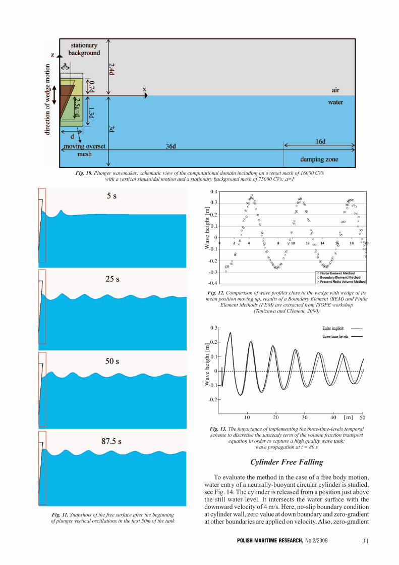
31POLISH MARITIME RESEARCH, No 2/2009
Fig. 10. Plunger wavemaker; schematic view of the computational domain including an overset mesh of 16000 CVs with a vertical sinusoidal motion and a stationary background mesh of 75000 CVs; a=1
Fig. 11. Snapshots of the free surface after the beginning of plunger vertical oscillations in the first 50m of the tank
Cylinder Free Falling
To evaluate the method in the case of a free body motion, water entry of a neutrally-buoyant circular cylinder is studied, see Fig. 14. The cylinder is released from a position just above the still water level. It intersects the water surface with the downward velocity of 4 m/s. Here, no-slip boundary condition at cylinder wall, zero value at down boundary and zero-gradient at other boundaries are applied on velocity. Also, zero-gradient
Fig. 12. Comparison of wave profiles close to the wedge with wedge at its mean position moving up; results of a Boundary Element (BEM) and Finite
Element Methods (FEM) are extracted from ISOPE workshop (Tanizawa and Clément, 2000)
Fig. 13. The importance of implementing the three-time-levels temporal scheme to discretise the unsteady term of the volume fraction transport
equation in order to capture a high quality wave tank; wave propagation at t = 80 s
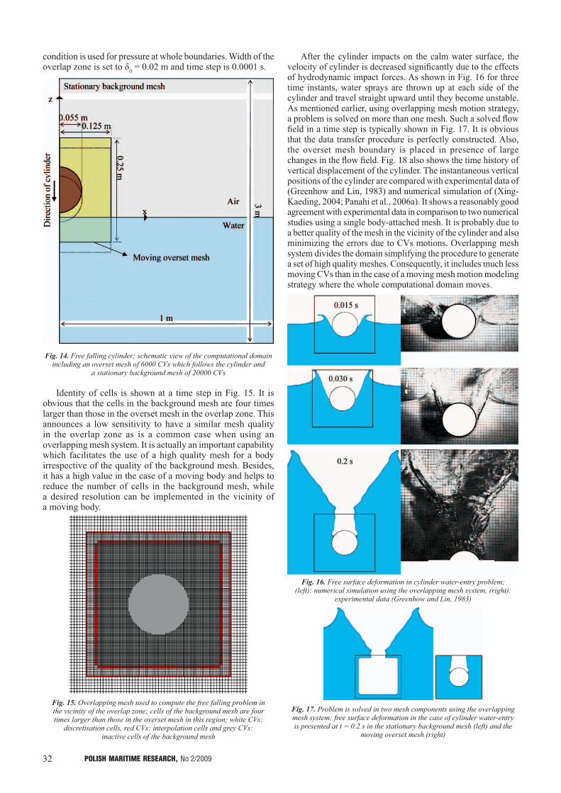
32 POLISH MARITIME RESEARCH, No 2/2009
condition is used for pressure at whole boundaries. Width of the overlap zone is set to δ0 = 0.02 m and time step is 0.0001 s.
Fig. 14. Free falling cylinder; schematic view of the computational domain including an overset mesh of 6000 CVs which follows the cylinder and
a stationary background mesh of 20000 CVs
Identity of cells is shown at a time step in Fig. 15. It is obvious that the cells in the background mesh are four times larger than those in the overset mesh in the overlap zone. This announces a low sensitivity to have a similar mesh quality in the overlap zone as is a common case when using an overlapping mesh system. It is actually an important capability which facilitates the use of a high quality mesh for a body irrespective of the quality of the background mesh. Besides, it has a high value in the case of a moving body and helps to reduce the number of cells in the background mesh, while a desired resolution can be implemented in the vicinity of a moving body.
Fig. 15. Overlapping mesh used to compute the free falling problem in the vicinity of the overlap zone; cells of the background mesh are four times larger than those in the overset mesh in this region; white CVs:
discretisation cells, red CVs: interpolation cells and grey CVs: inactive cells of the background mesh
After the cylinder impacts on the calm water surface, the velocity of cylinder is decreased significantly due to the effects of hydrodynamic impact forces. As shown in Fig. 16 for three time instants, water sprays are thrown up at each side of the cylinder and travel straight upward until they become unstable. As mentioned earlier, using overlapping mesh motion strategy, a problem is solved on more than one mesh. Such a solved flow field in a time step is typically shown in Fig. 17. It is obvious that the data transfer procedure is perfectly constructed. Also, the overset mesh boundary is placed in presence of large changes in the flow field. Fig. 18 also shows the time history of vertical displacement of the cylinder. The instantaneous vertical positions of the cylinder are compared with experimental data of (Greenhow and Lin, 1983) and numerical simulation of (Xing-Kaeding, 2004; Panahi et al., 2006a). It shows a reasonably good agreement with experimental data in comparison to two numerical studies using a single body-attached mesh. It is probably due to a better quality of the mesh in the vicinity of the cylinder and also minimizing the errors due to CVs motions. Overlapping mesh system divides the domain simplifying the procedure to generate a set of high quality meshes. Consequently, it includes much less moving CVs than in the case of a moving mesh motion modeling strategy where the whole computational domain moves.
Fig. 16. Free surface deformation in cylinder water-entry problem; (left): numerical simulation using the overlapping mesh system, (right):
experimental data (Greenhow and Lin, 1983)
Fig. 17. Problem is solved in two mesh components using the overlapping mesh system; free surface deformation in the case of cylinder water-entry is presented at t = 0.2 s in the stationary background mesh (left) and the
moving overset mesh (right)

33POLISH MARITIME RESEARCH, No 2/2009
Fig. 18. Time history of the cylinder water-entry just after the impact
CONCLUSION
As a complementary tool to marine laboratory tests, CFD proposes the ability to study a wide variety of hydrodynamic problems using an integrated method. Here, an algorithm among such possibilities is developed based on FV overlapping mesh system to deal with two-phase flow interaction with a structure. Selected test cases are good problems to assess different aspects of the proposed method. It can be simply developed to solve more complete problems especially to record hydrodynamics behavior of more than one structure in a numerical wave tank. Besides, the algorithm can be easily extended to 3D problems.
BIBLIOGRAPHY
1. Atta E.H.: Component adaptive grid interfacing. AIAA Paper, 81-0382, 1981
2. Blades E., Marcum D.L.: A sliding interface method for unsteady unstructured flow simulations. International Journal for Numerical Methods in Fluids, 2007
3. Buning P.G., Wong T.C., Dilley A.D., Pao J.L.: Prediction of hyper-x stage separation aerodynamics using CFD. AIAA Paper, 2000-4009, 2000
4. Carrica P.M., Wilson R.V., Noack R.W., Stern F.: Ship motions using single-phase level set with dynamic overset grids. Computers & Fluids, 36(9), 2007
5. Chen H.C., Lin W.M., Hwang W.Y.: Validation and application of chimera RANS method for ship-ship interactions in shallow water and restricted waterway. 24th ONR Symposium on Naval Hydrodynamics, Fukuoka, Japan, 2002
6. Chentanez N., Goktekin T.G., Feldman B.E., O’Brien J.F.: Simultaneous coupling of fluids and deformable bodies. Proceedings of the 2006 ACM SIGGRAPH/Eurographics Symposium on Computer Animation, 2006
7. Drakakis D., Majewski J., Rokichki J., Zoltak J.: Investigation of blending-function-based overlapping-grid technique for compressible flows. Computer Methods in Applied Mechanics and Engineering. 190, 2001
8. Ferziger J., Peric M.: Computational methods for fluid dynamics. 3rd Rev. Ed., Springer Verlag, 2002
9. Greenhow M., Lin W.: Nonlinear free surface effects: experiments and theory. Report No. 83-19, Massachusette Institute of Technology, 1983
10. Hadzic H.: Development and application of a finite volume method for the computation of flows around moving bodies on unstructured, overlapping grids. PhD Thesis, Teschnichen Universitat Hamburg-Harburg, 2005
11. Jahanbakhsh E., Panahi R., Seif M.S.: Numerical simulation of three-dimensional interfacial flows. International Journal of Numerical Methods for Heat & Fluid Flow, 17(4), 2007
12. Jahanbakhsh E., Panahi R., Seif M.S.: Catamaran motion simulation based On moving grid technique. Journal of Marine Science and Technology, Accepted for Publication, June 2008
13. Jasak H.: Error analysis and estimation for finite volume method with application to fluid flows. PhD Thesis, University of London, 1996
14. Kim D., Choi H.: A second-order time-accurate finite volume method for unsteady incompressible flow on hybrid unstructured grids. Journal of Computational Physics, 162(2), 2000
15. Löhner R.: Robust, vectorized search algorithms for interpolation on unstructured grids. Journal of Computational Physics, 118(2), 1995
16. Meakin R.L.: Object X-rays cutting holes in composite overset structured grids. AIAA Paper, 2001-2537, 2001
17. Mittal M., Iaccarino G.: Immersed boundary methods. Annual Review of Fluid Mechanics, 37, 2005
18. Nakahashi K., Togashi F., Sharov, D.: An intergrid-boundary definition method for overset unstructured grid approach. AIAA Journal, 38(11), 2000
19. Panahi R., Jahanbakhsh E., Seif M.S.: Comparison of interface capturing methods in two phase flow. Iranian Journal of Science & Technology, Transaction B: Technology, Vol.29, No.B6, 2005
20. Panahi R., Jahanbakhsh E., Seif M.S.: Development of a VoF fractional step solver for floating body motion simulation. Applied Ocean Research, 28(3), 2006a
21. Panahi R., Jahanbakhsh E., Seif M.S.: Numerical investigation on the effect of baffle arrangement in tanker sloshing. 9th Numerical Towing Tank Symposium (NuTTs), Nantes, France, 2006b
22. Park J.C., Miyata H.: Numerical simulation of fully-nonlinear wave motions around arctic and offshore structures. Journal of the Society of Naval Architects of Japan, 189, 2001
23. Schäfer M., Turek S.: Benchmark computations of laminar flow around a cylinder [J]. Notes on Numerical Fluid Mechanics, 52, 1996
24. Suhs N.E., Rogers S.E., Dietz W.E.: PEGASUS: An Automated pre-processor for overset grid CFD. AIAA Paper, 2002-3186, 2002
25. Tanizawa K., Clément A.H.: Report of the 2nd workshop of ISOPE numerical wave tank group: benchmark test cases of radiation problem. 10th International Offshore and Polar Engineering Conference, Seattle, USA, 2000
26. Togashi F., Nakahashi K., Ito Y., Iwamiyata T., Shimbo Y.: Flow simulation of NAL experimental supersonic airplane/booster separation using overset unstructured grids. Computers and Fluids, 30(6), 2001
27. Tremel U., Sorensen K.A., Hitzel S., Rieger H., Hassan O., Weatherill N.P.: Parallel remeshing of unstructured volume grids for CFD applications. International Journal for Numerical Methods in Fluids, 53(8), 2007
28. Ubbink O., Issa R.I.: A method for capturing sharp fluid interfaces on arbitrary meshes. Journal of Computational Physics, 153(1), 1999
29. Xing-Kaeding Y.: Unified approach to ship seakeeping and maneuvering by a RANSE method. PhD Thesis, Teschnichen Universitat Hamburg-Harburg, 2004.
CONTACT WITH THE AUTHORS
Roozbeh Panahi, Assoc. Prof.Mehdi Shafieefar, Assoc. Prof.Civil Engineering Department,
Tarbiat Modares University, P.O. Box: 14155-4838, Tehran, Iran,
tel: +9821 82883318, fax: +9821 82883538,
email: [email protected]

34 POLISH MARITIME RESEARCH, No 2/2009
INTRODUCTION
The design of ducted propellers is based on the same requirements and assumptions that were used in the design of open propellers [1,6]. The design procedure should lead to the compromise selection of the number and geometry of the propeller blades in order to ensure: the appropriate strength of the propeller blades the highest possible propulsive efficiency the absence of cavitation or only its limited presence, not
leading to erosion, vibration and noise the acceptable level of propeller-induced pressure pulses
on the hull the acceptable level of the unsteady bearing forces
The presence of the duct leads to the additional requirements: the appropriate selection of the duct geometry computation of the thrust generated by the duct computation of the velocity field generated by the duct
at the propeller, both for the propeller design and for the analysis of propeller operation in the non-uniform velocity field behind the ship hull.
Similarly as in the case of an open propeller, the complete design system for the ducted propellers should incorporate 3 interacting programs (i.e. 3 blocks of procedures):� programs for the determination of the design velocity
field
Tadeusz Koronowicz, Prof.Zbigniew Krzemianowski, Ph. D.Teresa Tuszkowska, Ph. D.The Szewalski Institute of Fluid Flow Machineryof the Polish Academy of Sciences in GdanskJan A. Szantyr, Prof.Gdansk University of Technology
� programs for the design of ducted propellers� programs for the analysis of the ducted propellers operation
in the non-uniform velocity field.
Moreover, the system should include the databases and graphical procedures for the selection of the duct geometry and procedures for calculation of the hydrodynamic forces and the velocity field generated by the duct. With reference to the system for open propellers design, the ducted propellers design system is supplemented with the following components:� graphical presentation of the available duct geometries in
order to facilitate duct selection� procedures for determination of the design velocity field and
of the axial hydrodynamic force generated by the duct� procedure for the duct-induced modification of the velocity
field on input to the program UNCA� procedure for determination of the pressure pulses generated
by the propeller around the duct-propeller system (based on the program UNCA)
� program for calculation of the pressure pulses generated by the duct (based on the program DUNCAN).
The appropriate interaction between the respective programs and procedures, supplemented with the above listed components, enables the complete design calculation of the ducted propeller. The presented program incorporates all necessary components integrated into one system and the design calculation may be controlled directly from the computer
A complete design of ducted propellers using the new computer system
ABSTRACT
The computer system for the completed design of the ducted ship propellers has some common blocks and procedures with the analogical system for open propellers that has already been presented in detail in the Polish Maritime Research [1]. This article describes only these blocks and procedures which are specific for the design of ducted propellers. These new blocks concern first of all the procedures for the design calculation of ducted propellers and for the analysis of the ducted propeller operation in the non-uniform velocity field behind the ship hull. The comparative analysis of computation results for different types of
ducts is also presented.
Keywords: ship propellers; ducted propellers; design methods; computational fluid dynamics
POLISH MARITIME RESEARCH 2(60) 2009 Vol 16; pp. 34-3910.2478/v10012-008-0019-3
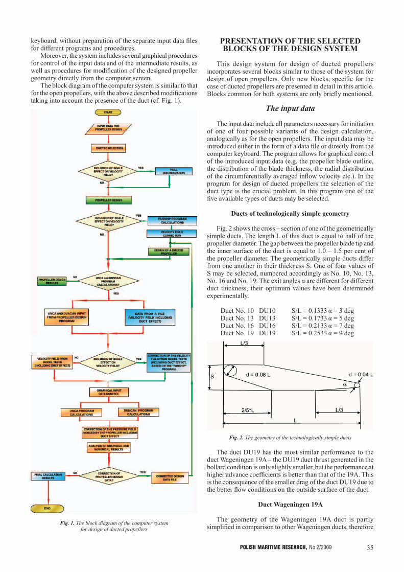
35POLISH MARITIME RESEARCH, No 2/2009
keyboard, without preparation of the separate input data files for different programs and procedures.
Moreover, the system includes several graphical procedures for control of the input data and of the intermediate results, as well as procedures for modification of the designed propeller geometry directly from the computer screen.
The block diagram of the computer system is similar to that for the open propellers, with the above described modifications taking into account the presence of the duct (cf. Fig. 1).
Fig. 1. The block diagram of the computer system for design of ducted propellers
PRESENTATION OF THE SELECTED BLOCKS OF THE DESIGN SYSTEM
This design system for design of ducted propellers incorporates several blocks similar to those of the system for design of open propellers. Only new blocks, specific for the case of ducted propellers are presented in detail in this article. Blocks common for both systems are only briefly mentioned.
The input data
The input data include all parameters necessary for initiation of one of four possible variants of the design calculation, analogically as for the open propellers. The input data may be introduced either in the form of a data file or directly from the computer keyboard. The program allows for graphical control of the introduced input data (e.g. the propeller blade outline, the distribution of the blade thickness, the radial distribution of the circumferentially averaged inflow velocity etc.). In the program for design of ducted propellers the selection of the duct type is the crucial problem. In this program one of the five available types of ducts may be selected.
Ducts of technologically simple geometry
Fig. 2 shows the cross – section of one of the geometrically simple ducts. The length L of this duct is equal to half of the propeller diameter. The gap between the propeller blade tip and the inner surface of the duct is equal to 1.0 – 1.5 per cent of the propeller diameter. The geometrically simple ducts differ from one another in their thickness S. One of four values of S may be selected, numbered accordingly as No. 10, No. 13, No. 16 and No. 19. The exit angles α are different for different duct thickness, their optimum values have been determined experimentally.
Duct No. 10 DU10 S/L = 0.1333 α = 3 deg Duct No. 13 DU13 S/L = 0.1733 α = 5 deg Duct No. 16 DU16 S/L = 0.2133 α = 7 deg Duct No. 19 DU19 S/L = 0.2533 α = 9 deg
Fig. 2. The geometry of the technologically simple ducts
The duct DU19 has the most similar performance to the duct Wageningen 19A – the DU19 duct thrust generated in the bollard condition is only slightly smaller, but the performance at higher advance coefficients is better than that of the 19A. This is the consequence of the smaller drag of the duct DU19 due to the better flow conditions on the outside surface of the duct.
Duct Wageningen 19A
The geometry of the Wageningen 19A duct is partly simplified in comparison to other Wageningen ducts, therefore

36 POLISH MARITIME RESEARCH, No 2/2009
this duct is the most frequently used one. Similarly as above, the duct length L is equal to half of the propeller diameter. The gap between the propeller blade tip and the inner surface of the duct is equal to 1 per cent of the propeller diameter. The non-dimensional ordinates of the duct profile (related to the duct length) are given in Tab. 1.
The design program
The algorithm for design of ducted propellers differs from the algorithm for design of open propellers presented in [1] only in a few details. The program based on this algorithm has been used for many years and it is thoroughly verified. The differing details are:� the calculations are conducted only for a given value of the
total thrust� the program automatically divides the total thrust into
parts generated by the propeller and by the duct. The part generated by the duct depends on the selected duct geometry and on the duct loading coefficient
� the inflow velocity field at the propeller is corrected by including the velocity field induced by the duct.
The missing possibility for calculating the ducted propeller for a given power (available in design of open propellers) may be balanced by performing calculations for several values of thrust and attaining the required power in an iterative process. In the case of open propellers such an iterative process is performed automatically.
The design calculation of a ducted propeller is performed always in the same way, irrespective of the selected version of calculations. This calculation ends with the results presented in the form of a numerical file describing the designed propeller and corresponding drawings on the computer screen (the drawings may be printed and/or stored in computer memory). Fig. 4 shows an example of such a drawing, which may be viewed on the screen from arbitrarily selected angles and the most interesting view may be designated for printing.
The program for the analysis of propeller operation in the non-uniform velocity field
The computer program UNCA for the analysis of the propeller operation in the non-uniform velocity field is a very important part of the system. The crucial part of this program is the determination of the extent and intensity of different
forms of cavitation on the blades of the propeller operating in the non-uniform inflow field. The original theoretical model integrates the unsteady vortex lifting surface theory with the unsteady sheet cavity theory. The detailed description of this algorithm is presented in [4, 5]. Additionally, the program DUNCAN [6] for calculation of the unsteady pressure pulses generated by the duct was included in the system.
The newly designed ducted propeller is checked by means of the UNCA and DUNCAN programs from the point of view of:� the detection of different forms of cavitation in different
angular position of the propeller blades in the ship hull wake
� the values of the pressure pulses generated on the hull surface or in the surrounding space. These pressure pulses are composed of these generated by the propeller (program UNCA) and by the duct (program DUNCAN)
� the values of unsteady bearing forces and moments.
After analyzing the above results the appropriate modifications of the propeller may be introduced and the design calculation may be repeated until the optimum result is obtained. For example the following parameters of the propeller may be modified:
Tab. 1. The ordinates of the profile of the Wageningen 19A duct
x/L 0 0.0125 0.025 0.05 0.1 0.2 0.3 0.4 0.5 0.6 0.7 0.8 0.9 0.95 1Yg/L 0.2025 0.2265 0.23 0.228 0.2204 0.2052 0.19 0.1748 0.1596 0.1444 0.1292 0.114 0.0988 0.0912 0.0836Yd/l 0.2025 0.1666 0.148 0.1212 0.0834 0.0417 0.0248 0.02 0.02 0.02 0.0229 0.0282 0.0345 0.0386 0.0436
Fig. 3. The geometry of the Wageningen 19A duct
Fig. 4. The view of the designed ducted propeller

37POLISH MARITIME RESEARCH, No 2/2009
� the values and radial distribution of the blade skew� the values and radial distribution of the blade section profile
lengths� the values and radial distribution of the blade section profile
maximum thicknesses� the type of the chord-wise thickness distribution� the type of the profile mean line� the radial distribution of the hydrodynamic loading
(circulation)� the number of blades� the type of duct.
The analysis of propeller operation in the non-uniform velocity field may be performed either for the propeller design condition (advance velocity and number of revolutions) or for off-design conditions without changing the propeller geometry and the velocity field. This option is convenient when compromise propellers for tugboats, fishing vessels and navy ships are designed. For these types of ships there are several different values of the operational velocity and all these conditions must be taken into account in the design process in order to obtain the optimum design.
The results of the cavitation analysis are presented in Fig. 5, while the results of calculation of the unsteady bearing forces and moments are given in Figs. 6-8.
Fig. 5. An example of presentation of the different calculated forms of cavitation on the propeller blades
Fig. 6. The components of the calculated unsteady bearing forces for a ducted propeller
COMPARATIVE ANALYSIS OF THE RESULTS
It is generally accepted that ducted propellers demonstrate increased efficiency and operational advantages only for ships with high pull at low speed (tugboats, fishing vessels etc.). Because of that, the most widely known and applied duct is the
Wageningen 19A, which was designed specifically for high pull at low speed. In the 1970s and 1980s a series of technologically simple ducts was developed at the Institute of Fluid Flow Machinery in Gdansk [3] (cf. Fig. 2). An extensive program of model experiments was performed in order to achieve the optimum duct geometry for different operating conditions. The optimum shape of the outer and inner parts of the duct was determined and the optimum values of the diffuser angle were obtained. It was discovered that the geometry of the outer part of the duct has a strong influence on the duct resistance. The purely conical shape of this part, as in the duct 19A, may lead to almost twofold increase in the duct resistance. Fig. 9 shows the hydrodynamic characteristics of all five ducts presented in Section 2. All presented results were obtained with the same propeller.
Fig. 7. The components of the calculated unsteady bearing moments for a ducted propeller
Fig. 8. The harmonic amplitudes of the bearing forces and moments for a ducted propeller
Fig. 9. The hydrodynamic characteristics of the ducted propeller for 5 ducts
As may be seen in the figure, the duct 19A has visibly higher negative thrust at high advance coefficients J. According to the research, the duct resistance coefficient CRD may be relatively

38 POLISH MARITIME RESEARCH, No 2/2009
only at the highest speed the open propeller is better. Both at medium and low speed the ducted propellers have a substantial advantage. Moreover, at high ship speed the ducted propellers may demonstrate other advantages: their optimum diameter is smaller and the amplitudes of the propeller-induced pressure pulses on the hull may be also smaller. Figs. 11 and 12 present the results of calculations (programs UNCA and DUNCAN) of the harmonic amplitudes of the induced pressure pulses on the hull for the ducted propeller DU13 (Fig. 11) and for the corresponding open propeller (Fig. 12). It is visible that the open propeller induces smaller pressure pulses.
Fig. 12. Harmonic amplitudes of the induced pressure pulses for the open propeller
FINAL REMARKS
� The above presented design system should significantly facilitate the process of design of ducted propellers. The system includes all components necessary in the correct process of design of propellers operating in the ducts of selected geometry (out of five options presented in Section 2.1 above). The available variants of the duct geometry enable design of high performance ducted propellers in a wide range of the operating conditions – even for relatively fast ships.
� There is a widely accepted opinion that the application of the ducted propellers is advantageous only in the case of high loading and low speed (tugs, trawlers etc.). This results from the fact that in most cases only the Wageningen 19A duct was considered and this duct was designed for low speed and high bollard pull conditions.
� The comparative analysis presented in the preceding Section shows, that the ducted propellers may offer competitive performance to open propellers and they may be successfully applied on ships with high speed. It should be pointed out that due to the danger of the propeller tip vortex cavitation and associated erosion on the inner surface of the duct, the Kaplan type blade outline for ducted propellers should be avoided.
BIBLIOGRAPHY
1. Koronowicz T., Krzemianowski Z., Tuszkowska T., Szantyr J.A.: A Complete Design of Ship Propellers Using the New Computer System, Polish Maritime Research No. 1 Vol. 16 (2009)
2. Koronowicz T.: The Algorithm of the Design Program Based on the Single Layer Lifting Surface for the Highly Skewed Propellers (in Polish), Report of the IFFM No. 296/86
accurately determined from the value of the duct thrust KTD corresponding to the zero propeller thrust:
The higher resistance of the duct 19A implies that it is the duct designed for high pull at low speed (in such conditions the high duct resistance ceases to influence visibly the characteristics). The relatively low resistance of the duct series DU allows them to be applied at higher values of the advance coefficient J. Fig. 10 shows the comparison of the calculated absorbed power for five ducts and for the open propeller.
Fig. 10. Comparison of the calculated absorbed power for the ducted propellers and for the open propeller
The above described computer system was used for designing all propellers in Fig. 10 for the given rate of rotation n = 120 rpm and for the required thrust T = 1500 kN. The diameter of respective propellers was determined as optimum in each case. For ducted propellers it was around 6.5 m, and for the open propeller it was equal to 7.23 m. The calculations were performed for three values of the inflow velocity: 2, 12 and 20 knots. In order to eliminate the influence of the velocity field (which is more positive for smaller propeller diameters), all calculations were conducted for the uniform inflow.
Fig. 11. Harmonic amplitudes of the induced pressure pulses for the DU13 ducted propeller
The analysis of the results presented In Fig. 10 leads to the conclusion, that as could be expected, the 19A duct performs better (i.e. absorbs less power) only at low inflow speeds. The ducts of the DU series demonstrate similar characteristics, but at low speed the duct DU19 is better, while at high speed the duct DU10 consumes less power. Very interesting conclusions may be drawn from comparison with the open propeller. Namely,

39POLISH MARITIME RESEARCH, No 2/2009
3. Koronowicz T.: Design of Ducted Propellers of Technologically Simple Geometry (in Polish), Proc. 5th Symposium of Ship Hydromechanics, Gdansk 1979
4. Szantyr J. A.: A Computer Program for Calculation of Cavitation Extent and Excitation Forces for a Propeller Operating in the Non-Uniform Velocity Field, International Shipbuilding Progress, No. 296, Vol. 26 (1979)
5. Szantyr J. A.: A Method for Analysis Cavitating Marine Propellers in Non-Uniform Flow, International Shipbuilding Progress, No. 427, Vol. 41 (1994)
6. Szantyr J. A.; User Instruction for the Program DUNCAN for the Analysis of Ducted Propellers Operating in Non-Uniform Velocity Field (in Polish), Report of the IFFM No. 150/88
7. Koronowicz T., Tuszkowska T., Waberska G., Krzemianowski Z., Chaja P., Góralczyk A.: The Design Algorithm for Screw Propellers (in Polish), Report of the IFFM No. 6103/06
8. Koronowicz T., Krzemianowski Z., Tuszkowska T., Góralczyk A.: The System of Programs for Design of Ducted Propellers(in Polish), Report of the IFFM No. 345/08
9. Koronowicz T., Szantyr J.A., Krzemianowski Z., Tuszkowska T., Waberska G.: The System of Programs for Design of Ship Propellers (in Polish), Report of the IFFM No. 148/08
10. Koronowicz T., Szantyr J. A., Chaja P.: A Computer System for the Complete Design of Ship Propellers, Proc. XVII International Conference on Hydrodynamics in Ship Design, Polanica, Poland, September 19th – 21st, 2007
11. Koronowicz T., Krzemianowski Z., Szantyr J. A.: Numerical Determination of the Propeller Design Velocity Field Including Scale Effect and Rudder Influence, Proc. 11th Numerical Towing Tank Symposium, Brest, France September 7th – 9th 2008
CONTACT WITH THE AUTHORS
Tadeusz Koronowicz, Prof.Zbigniew Krzemianowski, Ph. D.
Teresa Tuszkowska, Ph. D.Institute of Fluid-Flow Machinery,
Polish Academy of SciencesFiszera 14
80-952 Gdańsk, POLANDe-mail : [email protected]
Jan A. Szantyr, Prof. Department of Turbomachinery
and Fluid Mechanics,Gdańsk University of Technology
Narutowicza 11/1280-958 Gdańsk, POLAND
e-mail : [email protected]

40 POLISH MARITIME RESEARCH, No 2/2009
INTRODUCTION
Engines which are frequently used in the main propulsion systems on ships are large-power low-speed engines. Their efficiency reaches 48-51%, while large volumes of heat leave the engine with the exhaust gas. This heat can be a subject of further utilisation. Ref. [3] presents calculations of a combined power plant which consists of the main engine and the steam turbine circuit. The authors have proved that in this system, for the fuel consumption identical as for the conventional power plant the power output is increased by about 7%, while the specific fuel consumption decreases by, approximately, 6.5 %.
Due to their high efficiency, modern constructions of piston engine turbochargers do not require large volumes of exhaust gases. This provides opportunities for using a combined system which consists of an diesel engine, a power turbine, and a steam turbine.
In this situation two arrangements of the power turbine with the steam turbine are possible. In the first variant the diesel engine feeds in parallel the turbocharger and the power turbine with the exhaust gas taken from the main exhaust gas manifold. The exhaust gas from the power turbine and the turbocharger are then directed to the waste-heat boiler
On the possible increasing of efficiency of ship power plant with the system combined of marine diesel engine, gas turbine and steam turbine in case of main engine cooperation with the gas turbine fed in parallel and the steam turbine
Marek Dzida, Assoc. Prof. Janusz Mucharski, M. Sc.Gdansk University of Technology
ABSTRACT
The article presents a concept of a combined large-power ship propulsion system, composed of the leading internal combustion main engine associated with a power gas turbine and the steam turbine system, both utilising the energy taken from the main engine exhaust gas. In the examined variant the power turbine, arranged in parallel with a turbocharger, is fed with the exhaust gas from the exhaust manifold. A calculation algorithm is presented, along with sample calculations for particular subsystems: supercharging, gas power turbine, and steam turbine system. Assumptions were formulated for the calculations, and were complemented by the adopted limits. Selected system parameters were confronted with the experimental investigations available in the literature. The performed power optimisation of the entire combined marine power plant took only into account the thermodynamic point of view, leaving aside technical and economic
aspects. The numerical calculations were performed for the 52 MW low-speed marine diesel engine.
Keywords: marine power plants; combined systems; piston internal combustion engines; gas turbine; steam turbine
which produces the steam used by the steam turbine. In the second variant, the turbocharger and the power turbine are fed in series from the diesel engine exhaust gas manifold. The exhaust gas from the diesel engine does not expand entirely to the atmospheric pressure in the turbocharger but to a higher pressure, thus leaving part of the enthalpy drop to be utilised in the power turbine. From the power turbine the exhaust gas flows to the waste-heat boiler where its heat is taken over by the steam to be used in the steam turbine to produce additional power.
The article discusses a combined system of the main engine with a turbocharger and a power gas turbine, fed in parallel from the exhaust gas manifold, and the steam turbine system. The analysed combined propulsion system has the identical main engine as that discussed in Ref. [3]. The present system was only analysed with respect to thermodynamic aspects of its application as a combined propulsion system. The required power of the gas turbine was determined for the assumed efficiencies of the turbocharger and the power turbine, while the steam turbine cycle was optimised to obtain the maximum power, assuming the use of the two-pressure waste-heat boiler. The optimisation of the steam turbine system took into account limitations resulting from practical designs used in real propulsion systems.
POLISH MARITIME RESEARCH 2(60) 2009 Vol 16; pp. 40-4410.2478/v10012-008-0020-x
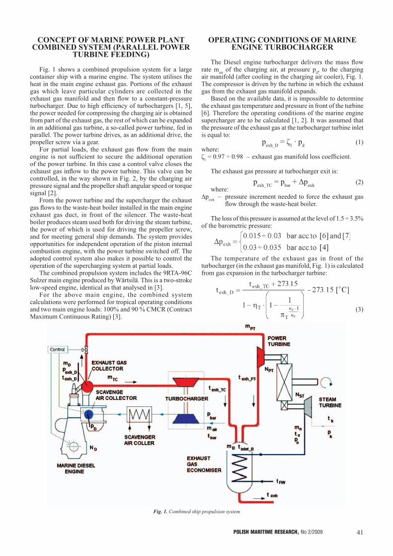
41POLISH MARITIME RESEARCH, No 2/2009
CONCEPT OF MARINE POWER PLANT COMBINED SYSTEM (PARALLEL POWER
TURBINE FEEDING)
Fig. 1 shows a combined propulsion system for a large container ship with a marine engine. The system utilises the heat in the main engine exhaust gas. Portions of the exhaust gas which leave particular cylinders are collected in the exhaust gas manifold and then flow to a constant-pressure turbocharger. Due to high efficiency of turbochargers [1, 5], the power needed for compressing the charging air is obtained from part of the exhaust gas, the rest of which can be expanded in an additional gas turbine, a so-called power turbine, fed in parallel. The power turbine drives, as an additional drive, the propeller screw via a gear.
For partial loads, the exhaust gas flow from the main engine is not sufficient to secure the additional operation of the power turbine. In this case a control valve closes the exhaust gas inflow to the power turbine. This valve can be controlled, in the way shown in Fig. 2, by the charging air pressure signal and the propeller shaft angular speed or torque signal [2].
From the power turbine and the supercharger the exhaust gas flows to the waste-heat boiler installed in the main engine exhaust gas duct, in front of the silencer. The waste-heat boiler produces steam used both for driving the steam turbine, the power of which is used for driving the propeller screw, and for meeting general ship demands. The system provides opportunities for independent operation of the piston internal combustion engine, with the power turbine switched off. The adopted control system also makes it possible to control the operation of the supercharging system at partial loads.
The combined propulsion system includes the 9RTA-96C Sulzer main engine produced by Wärtsilä. This is a two-stroke low-speed engine, identical as that analysed in [3].
For the above main engine, the combined system calculations were performed for tropical operating conditions and two main engine loads: 100% and 90 % CMCR (Contract Maximum Continuous Rating) [3].
OPERATING CONDITIONS OF MARINE ENGINE TURBOCHARGER
The Diesel engine turbocharger delivers the mass flow rate mair of the charging air, at pressure pd, to the charging air manifold (after cooling in the charging air cooler), Fig. 1. The compressor is driven by the turbine in which the exhaust gas from the exhaust gas manifold expands.
Based on the available data, it is impossible to determine the exhaust gas temperature and pressure in front of the turbine [6]. Therefore the operating conditions of the marine engine supercharger are to be calculated [1, 2]. It was assumed that the pressure of the exhaust gas at the turbocharger turbine inlet is equal to:
pexh_D = ζ1 · pd (1)where:ζ1 = 0.97 ÷ 0.98 – exhaust gas manifold loss coefficient.
The exhaust gas pressure at turbocharger exit is:
pexh_TC = pbar + ∆pexh (2)where:
∆pexh – pressure increment needed to force the exhaust gas flow through the waste-heat boiler.
The loss of this pressure is assumed at the level of 1.5 ÷ 3.5% of the barometric pressure:
The temperature of the exhaust gas in front of the turbocharger (in the exhaust gas manifold, Fig. 1) is calculated from gas expansion in the turbocharger turbine:
(3)
Fig. 1. Combined ship propulsion system

42 POLISH MARITIME RESEARCH, No 2/2009
where:ηT – turbocharger turbine efficiencyπT = pinlet_TC / pexh_TC – turbine expansion ratio.
Fig. 2 presents temperature changes in the exhaust gas manifold: texh_D – (calculated) and the temperature of the exhaust gases
behind the turbocharger texh_TC – given by the producer [6], as a function of the main
engine load.
The exhaust gas flow needed for turbocharger operation is determined from the turbocharger power balance, Fig. 1, using the following formula:
(4)
where:ηTC = ηT · ηC · ηm – turbocharger efficiencyπC =pexh_C/pbar – turbocharger compressor compression
ratio.
From the turbocharger, the exhaust gas flow mTC having the temperature texh_TC is directed to the waste-heat boiler.
POWER TURBINE CALCULATIONS The power turbine is fed with the exhaust gas from the
exhaust gas manifold. The exhaust gas flow mPT has the temperature texh_D identical as that in the turbocharger, Fig. 1. The mass flow rate of the exhaust gas to the power turbine was calculated from the relation:
(5)
It was assumed in the cycle calculations that the exhaust gas at power turbine inlet and exit has the same pressure as in the turbocharger. The power output of the power turbine is calculated from the relation:
NPT = ηm · mPT · HPT (6)
where:ηm – mechanical efficiency of the power turbineHTM – enthalpy drop in the power turbine.
The temperature of the exhaust gas behind the power turbine is slightly higher than that behind the turbocharger, see relevant curves in Fig. 2. The increased load of the main engine results in the increase of both the temperature of the exhaust gas in the manifold, and the mass flow rate of the exhaust gas working in the power turbine. All this, as a final result, increases the turbine power.
Fig. 2. Power turbine parameters vs. main engine load
Increasing the power in the main engine turbine system results in the power increase amounting to about 2% for engine
loads of an order of 70%, and to over 8% for the maximal loads, accompanied by relevant reduction of the specific fuel consumption, respectively, from 2% to about 7.5%. It is also noteworthy that for the main engine power below 60-70% the operation of the power turbine is impossible. In this case the control system should close the valve which controls the exhaust gas inflow to the power turbine, Fig. 1.
STEAM TURBINE CALCULATIONS
The assumed two-pressure waste-heat boiler is identical with that analysed [3]. Fig. 3 presents a scheme of the steam system consisting of a steam turbine and a waste-heat boiler. Form the turbocharger and the power turbine the exhaust gas flows through the waste-heat boiler delivering the heat to the steam cycle. In the high-pressure cycle (pII) the superheated steam is produced, the parameters of which are (po, to) and the mass flow rate is mo. This steam flows to the steam turbine. The low-pressure cycle (pI) produces the saturated steam, the part mPW of which is taken to cover general ship needs, and the remaining part is delivered to the steam turbine increasing its power. The applied steam turbine is a condensation turbine which drives, as an additional drive, the ship propeller screw via a reduction gear. The assumed boiling type degasifier supplies the waste-heat boiler with water having the temperature tFW. The condensate flows to the degasifier from the condenser and from the heat box, a component of the general ship needs system. Additional heat needed for increasing the water temperature to the boiling temperature in the degasifier is taken from a steam turbine extraction point. The exhaust gas leaving the waste-heat boiler has the temperature texh. The temperature of the gas in front of the boiler is calculated from the balance of the mixture of gases from the turbocharger and from the power turbine.
(7)
Fig. 3. Scheme of the ship system consisting of a steam turbine and a waste-heat boiler

43POLISH MARITIME RESEARCH, No 2/2009
Steam cycle optimisation
The numerical calculations of the steam cycle were performed using the algorithm presented [3]. The calculations were performed in variants for: the assumed range of the high-pressure cycle pressure (live steam pressure) po ∈ ⟨po_min , po_max⟩, the assumed range of the low-pressure cycle pressure pI ∈ ⟨pI_min , pI_max⟩ and the assumed pressure range in the degasifier pg ∈ ⟨pg_min , pg_max⟩.
Tab. 1 collects optimum parameters of the steam cycle for two loads of the Diesel engine. The maximum power of the steam turbine, obtained from the optimisation calculations, is NSTmax = 3470 kW for the Diesel engine load equal to 90 %. This case did not take into account the adopted limits. In a real system, certain limits are to be taken into account in the ship steam cycle. For the assumed limits the maximum power of the steam cycle is NSTmax = 3075 kW. When a steam turbine was added to the Diesel engine system, the power output of the ship propulsion system was increased by ∆NST/ND = 7.37 % and 6.64 %, respectively for the 100 and 90 % load, at simultaneous reduction of the specific fuel consumption in the combined system, respectively, from 174 g/kWh to 162.1 g/kWh and from 169.8 g/kWh to 159.2 g/kWh, see Tab. 2. The specific fuel stream was decreased by 6.86 % for 100 % load and by 6.22 % for 90 % load of the diesel engine, as compared to the fuel consumption of the diesel engine alone.
In the steam system with the limits, the heat in the diesel engine exhaust gas is used, at 90 % load for instance, for the production of the live superheated steam mo = 12.9 t/h having parameters to = 289 °C and po = 25 bar, and the live wet steam mI = 9.30 t/h, having temperature tI = 165 °C and pressure pI = 7 bar, see Tab. 1.
THERMODYNAMIC ANALYSIS OF THE COMBINED CYCLE
The use of the combined ship propulsion system increases its efficiency, which leads to the decrease of the specific fuel consumption and the increase of the power, without delivery of additional fuel. Tab. 2 collects powers, efficiencies, and specific fuel consumptions for the examined combined ship propulsion system.
The use of the power turbine increases the power produced by the system by 2211 kW, i.e. by 4.77 % for the 90 % main engine load, and decreases the specific fuel consumption by 4.6 %, as compared to the classical propulsion system. Introducing a steam turbine to the combined system increases its power by 11.4 % and decreases its specific fuel consumption by 10.2 %. The efficiency of the combined propulsion system increases from 50 % to 55 %.
CONCLUSIONS � The proposed concept of a combined marine power plant
consisting of a low-speed marine diesel engine with a power turbine and steam turbine utilising the heat transported with the diesel engine exhaust gas decreases the specific fuel consumption of the plant by about 10 %. Moreover, without changing nominal power of the main engine the total power of the power plant is increased by about 11% due to the use of the waste heat in the exhaust gas. Simultaneously, the specific fuel consumption decreases by 10 ÷ 12 % as compared to the standard power plant.
� For marine power plants on large merchant ships with low-speed engines of power output over 50 MW, power plants of this type seem to be competitive with a traditional power plant.
Tab. 1. Optimal steam cycle parameters in the combined system consisting of the Diesel engine, power turbine (parallel feeding), and steam turbine
No ND[%]
to[°C]
po[bar]
pI[bar]
tI[°C]
pg[bar]
texh[°C]
tFW[°C] x mo
[t/h]mI
[t/h]mu
[t/h]NST
[kW] NST/ND
without limits1 100 299 27.0 7.0 165 0.50 153 82 0.8715 15.02 10.78 1.93 4073 0.07912 90 286 20.0 5.0 152 0.50 143 82 0.8796 0.037 0.03 0.005 3470 0.0749
with limits1 100 299 22.0 7.0 165 2.00 163 121 0.8800 0.042 0.025 0.009 3794 0.07372 90 286 19.0 7.0 165 2.00 164 121 0.8812 0.038 0.022 0.008 3075 0.0664
Tab. 2. Power, efficiency and specific fuel consumption for a combined ship propulsion system with a two-stroke engine 9RTA 96C, power turbine (parallel feeding) and steam turbine
No
RTA96C engine Diesel Engine& Power Turbine
Diesel Engine& Steam Turbine
Diesel Engine& Power Turbine& Steam Turbine
ND[%]
ND[kW]
NPT[kW]
∆NPT/ND[%]
NST[kW]
∆NST/ND[%]
Ncombi[kW]
∆Ncombi/ND[%]
1 100 51480 3203 6.22 3794 7.37 58477 13.592 90 46332 2211 4.77 3075 6.64 51618 11.41
ND[%]
ND[kW]
bed[g/kWh]
bePT[g/kWh]
∆bePT/beD[%]
beST[g/kWh]
∆beST/beD[%]
becombi[g/kWh]
∆becombi/beD[%]
1 100 51480 174.0 163.8 -5.86 162.1 -6.86 153.2 -11.972 90 46332 169.8 162.1 -4.56 159.2 -6.22 152.4 -10.24
ND[%]
ND[kW]
ηD[%]
ηPT[%]
∆ηPT/ηD[%]
ηST[%]
∆ηST/ηD[%]
ηcombi[g/kWh]
∆ηcombi/ηD[%]
1 100 51480 48.46 54.90 6.22 52.04 7.37 55.05 13.592 90 46332 49.66 55.53 4.77 52.96 6.64 55.33 11.41

44 POLISH MARITIME RESEARCH, No 2/2009
� At power load of 100 % CMCR, the engine 9RTA96C consumes 215 t/24h, while for the combined power plant the same power is obtained by the plant at the main engine load of 90 % CMCR and fuel consumption equal to 189 t/24h. This brings the ship owner measurable gains expressed in fuel consumption reduction by 26 t/24h.
NOMENCLATURE
be - specific fuel oil consumptioncg, ca - specific heat of exhaust gas and air, respectivelyi - specific enthalpym - mass flux of a medium N - powerp - pressureT, t - temperatureWu - calorific value of fuel oilη - efficiencyκg, κa - isentropic exponent of exhaust gas and air, respectively
Indicesbar - barometric conditionsB - boilercombi - combined systemD - marine diesel engine, superchargingf - fuelinlet - inlet passagek - parameters in a condensero - live steam, calculation pointair - airss - ship living purposesπ - stage of: compression in a compressor, decompression
in a turbineC - compressorg - exhaust gasT - turbine
TC - turbochargerPT - power turbineST - steam turbineexh - exhaust passageFW - water supplying a waste heat boiler
BIBLIOGRAPHY
1. A new turbocharger generation. ABB Turbo Systems Ltd. Publication No. CH-Z 2035 98E.
2. Description of Marine GenSet- Type L28/32H. MAN B&W Diesel A/S. November 1993.
3. Dzida M.: On the possible increasing of efficiency of ship power plant with the system combined of pi-ston combustion engine, gas turbine and steam turbine, at the main engine - steam turbine mode of cooperation. Polish Maritime Research No 1(59), Vol. 16, 2009
4. Kehlhofer R.: Combined-Cycle Gas & Steam Turbine Power Plants. The Fairmont Press, INC. USA. 1991.
5. Schrott K. H.: The New Generation of MAN B&W Turbochargers. MAN B&W Publication S.A. 236 5581E. 1995
6. Sulzer RTA 96C. Engine Selection and Project Manual. June 2001. Wärtsilä.
7. The MC Engine. Exhaust Gas Date. Waste Heat Recovery System. Total Economy. Publication MAN B&W. October 1985.
CONTACT WITH THE AUTHORS
Marek Dzida, Assoc. Prof.Faculty of Ocean Engineering
and Ship TechnologyGdansk University of Technology
Narutowicza 11/1280-233 Gdansk, POLANDe-mail: [email protected]
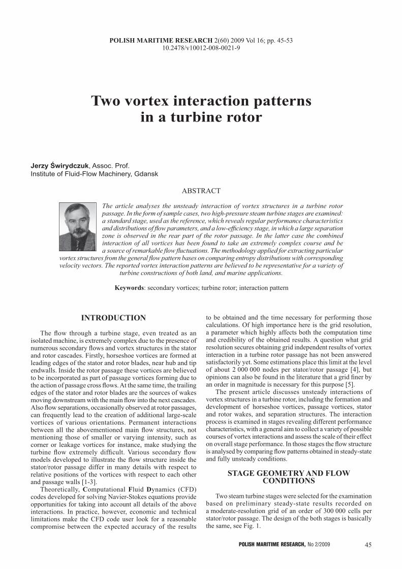
45POLISH MARITIME RESEARCH, No 2/2009
INTRODUCTION
The flow through a turbine stage, even treated as an isolated machine, is extremely complex due to the presence of numerous secondary flows and vortex structures in the stator and rotor cascades. Firstly, horseshoe vortices are formed at leading edges of the stator and rotor blades, near hub and tip endwalls. Inside the rotor passage these vortices are believed to be incorporated as part of passage vortices forming due to the action of passage cross flows. At the same time, the trailing edges of the stator and rotor blades are the sources of wakes moving downstream with the main flow into the next cascades. Also flow separations, occasionally observed at rotor passages, can frequently lead to the creation of additional large-scale vortices of various orientations. Permanent interactions between all the abovementioned main flow structures, not mentioning those of smaller or varying intensity, such as corner or leakage vortices for instance, make studying the turbine flow extremely difficult. Various secondary flow models developed to illustrate the flow structure inside the stator/rotor passage differ in many details with respect to relative positions of the vortices with respect to each other and passage walls [1-3].
Theoretically, Computational Fluid Dynamics (CFD) codes developed for solving Navier-Stokes equations provide opportunities for taking into account all details of the above interactions. In practice, however, economic and technical limitations make the CFD code user look for a reasonable compromise between the expected accuracy of the results
to be obtained and the time necessary for performing those calculations. Of high importance here is the grid resolution, a parameter which highly affects both the computation time and credibility of the obtained results. A question what grid resolution secures obtaining grid independent results of vortex interaction in a turbine rotor passage has not been answered satisfactorily yet. Some estimations place this limit at the level of about 2 000 000 nodes per stator/rotor passage [4], but opinions can also be found in the literature that a grid finer by an order in magnitude is necessary for this purpose [5].
The present article discusses unsteady interactions of vortex structures in a turbine rotor, including the formation and development of horseshoe vortices, passage vortices, stator and rotor wakes, and separation structures. The interaction process is examined in stages revealing different performance characteristics, with a general aim to collect a variety of possible courses of vortex interactions and assess the scale of their effect on overall stage performance. In those stages the flow structure is analysed by comparing flow patterns obtained in steady-state and fully unsteady conditions.
STAGE GEOMETRY AND FLOW CONDITIONS
Two steam turbine stages were selected for the examination based on preliminary steady-state results recorded on a moderate-resolution grid of an order of 300 000 cells per stator/rotor passage. The design of the both stages is basically the same, see Fig. 1.
Two vortex interaction patterns in a turbine rotor
Jerzy Świrydczuk, Assoc. Prof.Institute of Fluid-Flow Machinery, Gdansk
ABSTRACT
The article analyses the unsteady interaction of vortex structures in a turbine rotor passage. In the form of sample cases, two high-pressure steam turbine stages are examined: a standard stage, used as the reference, which reveals regular performance characteristics and distributions of flow parameters, and a low-efficiency stage, in which a large separation zone is observed in the rear part of the rotor passage. In the latter case the combined interaction of all vortices has been found to take an extremely complex course and be a source of remarkable flow fluctuations. The methodology applied for extracting particular
vortex structures from the general flow pattern bases on comparing entropy distributions with corresponding velocity vectors. The reported vortex interaction patterns are believed to be representative for a variety of
turbine constructions of both land, and marine applications.
Keywords: secondary vortices; turbine rotor; interaction pattern
POLISH MARITIME RESEARCH 2(60) 2009 Vol 16; pp. 45-5310.2478/v10012-008-0021-9
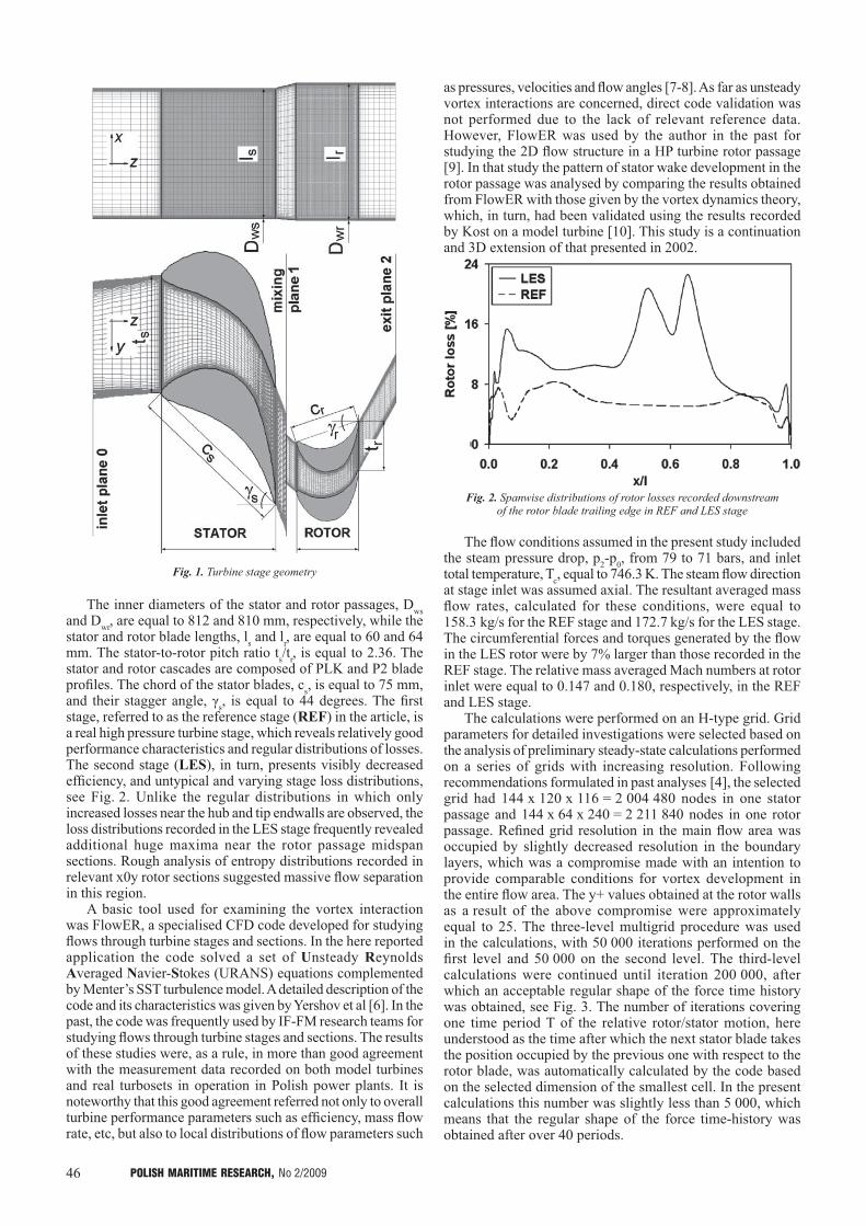
46 POLISH MARITIME RESEARCH, No 2/2009
Fig. 1. Turbine stage geometry
The inner diameters of the stator and rotor passages, Dws and Dwr, are equal to 812 and 810 mm, respectively, while the stator and rotor blade lengths, ls and lr, are equal to 60 and 64 mm. The stator-to-rotor pitch ratio ts/tr, is equal to 2.36. The stator and rotor cascades are composed of PLK and P2 blade profiles. The chord of the stator blades, cs, is equal to 75 mm, and their stagger angle, γs, is equal to 44 degrees. The first stage, referred to as the reference stage (REF) in the article, is a real high pressure turbine stage, which reveals relatively good performance characteristics and regular distributions of losses. The second stage (LES), in turn, presents visibly decreased efficiency, and untypical and varying stage loss distributions, see Fig. 2. Unlike the regular distributions in which only increased losses near the hub and tip endwalls are observed, the loss distributions recorded in the LES stage frequently revealed additional huge maxima near the rotor passage midspan sections. Rough analysis of entropy distributions recorded in relevant x0y rotor sections suggested massive flow separation in this region.
A basic tool used for examining the vortex interaction was FlowER, a specialised CFD code developed for studying flows through turbine stages and sections. In the here reported application the code solved a set of Unsteady Reynolds Averaged Navier-Stokes (URANS) equations complemented by Menter’s SST turbulence model. A detailed description of the code and its characteristics was given by Yershov et al [6]. In the past, the code was frequently used by IF-FM research teams for studying flows through turbine stages and sections. The results of these studies were, as a rule, in more than good agreement with the measurement data recorded on both model turbines and real turbosets in operation in Polish power plants. It is noteworthy that this good agreement referred not only to overall turbine performance parameters such as efficiency, mass flow rate, etc, but also to local distributions of flow parameters such
as pressures, velocities and flow angles [7-8]. As far as unsteady vortex interactions are concerned, direct code validation was not performed due to the lack of relevant reference data. However, FlowER was used by the author in the past for studying the 2D flow structure in a HP turbine rotor passage [9]. In that study the pattern of stator wake development in the rotor passage was analysed by comparing the results obtained from FlowER with those given by the vortex dynamics theory, which, in turn, had been validated using the results recorded by Kost on a model turbine [10]. This study is a continuation and 3D extension of that presented in 2002.
Fig. 2. Spanwise distributions of rotor losses recorded downstream of the rotor blade trailing edge in REF and LES stage
The flow conditions assumed in the present study included the steam pressure drop, p2-p0, from 79 to 71 bars, and inlet total temperature, Tc, equal to 746.3 K. The steam flow direction at stage inlet was assumed axial. The resultant averaged mass flow rates, calculated for these conditions, were equal to 158.3 kg/s for the REF stage and 172.7 kg/s for the LES stage. The circumferential forces and torques generated by the flow in the LES rotor were by 7% larger than those recorded in the REF stage. The relative mass averaged Mach numbers at rotor inlet were equal to 0.147 and 0.180, respectively, in the REF and LES stage.
The calculations were performed on an H-type grid. Grid parameters for detailed investigations were selected based on the analysis of preliminary steady-state calculations performed on a series of grids with increasing resolution. Following recommendations formulated in past analyses [4], the selected grid had 144 x 120 x 116 = 2 004 480 nodes in one stator passage and 144 x 64 x 240 = 2 211 840 nodes in one rotor passage. Refined grid resolution in the main flow area was occupied by slightly decreased resolution in the boundary layers, which was a compromise made with an intention to provide comparable conditions for vortex development in the entire flow area. The y+ values obtained at the rotor walls as a result of the above compromise were approximately equal to 25. The three-level multigrid procedure was used in the calculations, with 50 000 iterations performed on the first level and 50 000 on the second level. The third-level calculations were continued until iteration 200 000, after which an acceptable regular shape of the force time history was obtained, see Fig. 3. The number of iterations covering one time period T of the relative rotor/stator motion, here understood as the time after which the next stator blade takes the position occupied by the previous one with respect to the rotor blade, was automatically calculated by the code based on the selected dimension of the smallest cell. In the present calculations this number was slightly less than 5 000, which means that the regular shape of the force time-history was obtained after over 40 periods.

47POLISH MARITIME RESEARCH, No 2/2009
Fig. 3. Time-history of total force fluctuations in turbine rotor
STATOR WAKE AT ROTOR INLET
The examined stages are impulse stages. In those stages the major part of steam expansion is realised in the stator, and the main role of the rotor cascade is to reverse the flow. As a result, the flow changes its direction by less than 80 degrees (from axial to nearly circumferential) in the stator, and by as much as about 140 degrees in the rotor cascade. Since the intensities of secondary flow structures in turbine cascades are commonly believed to be in close relation with the above flow angle differences, much more intensive structures are expected to be recorded in the rotor.
Fig. 4 shows two selected instantaneous entropy distributions recorded inside and in front of the rotor cascade. The diagram on the left presents a typical flow pattern recorded at the rotor passage half-span section, with stator and rotor wakes being the only secondary flow structures. The flow pattern on the right was recorded at the rotor inlet, at a distance of 0.1 crz (crz - rotor blade chord projection onto the turbine axis) from rotor blade leading edges, when the stator wake occupied an approximate position in the middle between the rotor blades. The stator wake shown here is slightly inclined with respect to the radial direction, and has a regular shape along most of its length. Only near the endwalls, at an approximate distance of 0.05 lr (lr - rotor blade length) from the hub endwall, and about 0.15 lr from the tip endwall 15%, some traces of stator passage vortices can be noticed.
To check the relations between intensities of particular vortex structures observed at rotor inlet, a series of diagrams showing velocity distributions along selected y-lines located in the plane z/crz = -0.1 at different x/lr values has been prepared,
see Fig. 5. Different axis orientations of the vortex structures shown in the plane z/crz = -0.1 do not provide opportunities for selecting one leading velocity component and treat it as the representative material for studying vortex behaviour. That is why all three velocity components are presented in Fig. 5. The curves in each diagram compose two series, one of which represents the time instant of the current wake position shown in Fig. 4, while the other - their values averaged over the entire time period of relative stator/rotor motion. The observed differences between these curves are expected to reflect the effects generated by the vortex structures. Two continuous-line curves: the thick curve recorded at the time instant from Fig. 4 at the half-span section (x/lr = 0.50) and its thinner equivalent representing the averaged distribution, are given as the reference to illustrate velocity changes generated by the stator wake alone. Three remaining curves were been recorded at the characteristic sections: x/lr = 0.05 - stator hub passage vortex location, x/lr = 0.87 - stator tip passage vortex location, x/lr = 0.95 - no visible presence of any regular structures.
Analysing the REF curves (x/lr = 0.50) in the left-hand diagram leads to the conclusion that the action of the stator wake manifests itself in the presence of a disturbance having a sinusoidal shape. Starting from the left, the instantaneous velocity first increases above the averaged values, then decreases below and finally reaches again the level higher than the averaged curve. Disturbances of similar nature can be recognised in all remaining instant curves, the only difference being relative
Fig. 5. Distributions of velocity components in plane z/crz = -0.1: left - circumferential velocity, centre - axial velocity, right - radial velocity
Fig. 4. Stator wake patterns in y0z and x0y planes inside and in front of rotor passage
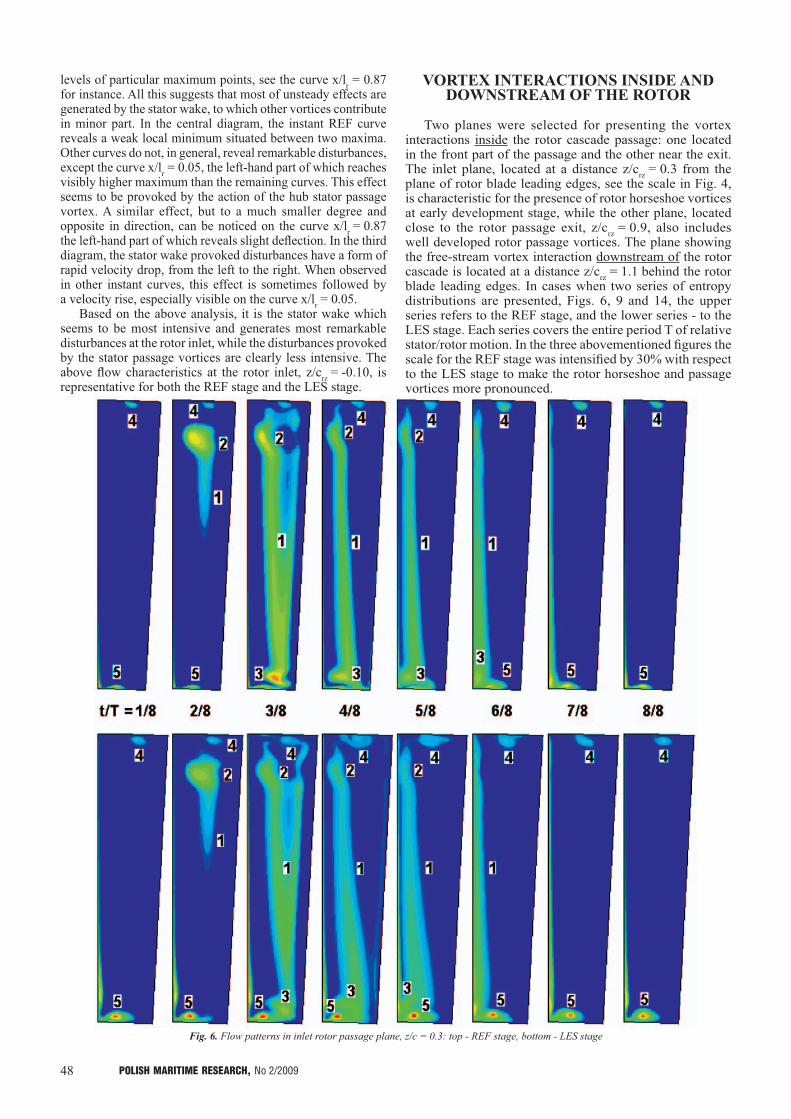
48 POLISH MARITIME RESEARCH, No 2/2009
levels of particular maximum points, see the curve x/lr = 0.87 for instance. All this suggests that most of unsteady effects are generated by the stator wake, to which other vortices contribute in minor part. In the central diagram, the instant REF curve reveals a weak local minimum situated between two maxima. Other curves do not, in general, reveal remarkable disturbances, except the curve x/lr = 0.05, the left-hand part of which reaches visibly higher maximum than the remaining curves. This effect seems to be provoked by the action of the hub stator passage vortex. A similar effect, but to a much smaller degree and opposite in direction, can be noticed on the curve x/lr = 0.87 the left-hand part of which reveals slight deflection. In the third diagram, the stator wake provoked disturbances have a form of rapid velocity drop, from the left to the right. When observed in other instant curves, this effect is sometimes followed by a velocity rise, especially visible on the curve x/lr = 0.05.
Based on the above analysis, it is the stator wake which seems to be most intensive and generates most remarkable disturbances at the rotor inlet, while the disturbances provoked by the stator passage vortices are clearly less intensive. The above flow characteristics at the rotor inlet, z/crz = -0.10, is representative for both the REF stage and the LES stage.
VORTEX INTERACTIONS INSIDE AND DOWNSTREAM OF THE ROTOR
Two planes were selected for presenting the vortex interactions inside the rotor cascade passage: one located in the front part of the passage and the other near the exit. The inlet plane, located at a distance z/crz = 0.3 from the plane of rotor blade leading edges, see the scale in Fig. 4, is characteristic for the presence of rotor horseshoe vortices at early development stage, while the other plane, located close to the rotor passage exit, z/crz = 0.9, also includes well developed rotor passage vortices. The plane showing the free-stream vortex interaction downstream of the rotor cascade is located at a distance z/crz = 1.1 behind the rotor blade leading edges. In cases when two series of entropy distributions are presented, Figs. 6, 9 and 14, the upper series refers to the REF stage, and the lower series - to the LES stage. Each series covers the entire period T of relative stator/rotor motion. In the three abovementioned figures the scale for the REF stage was intensified by 30% with respect to the LES stage to make the rotor horseshoe and passage vortices more pronounced.
Fig. 6. Flow patterns in inlet rotor passage plane, z/c = 0.3: top - REF stage, bottom - LES stage
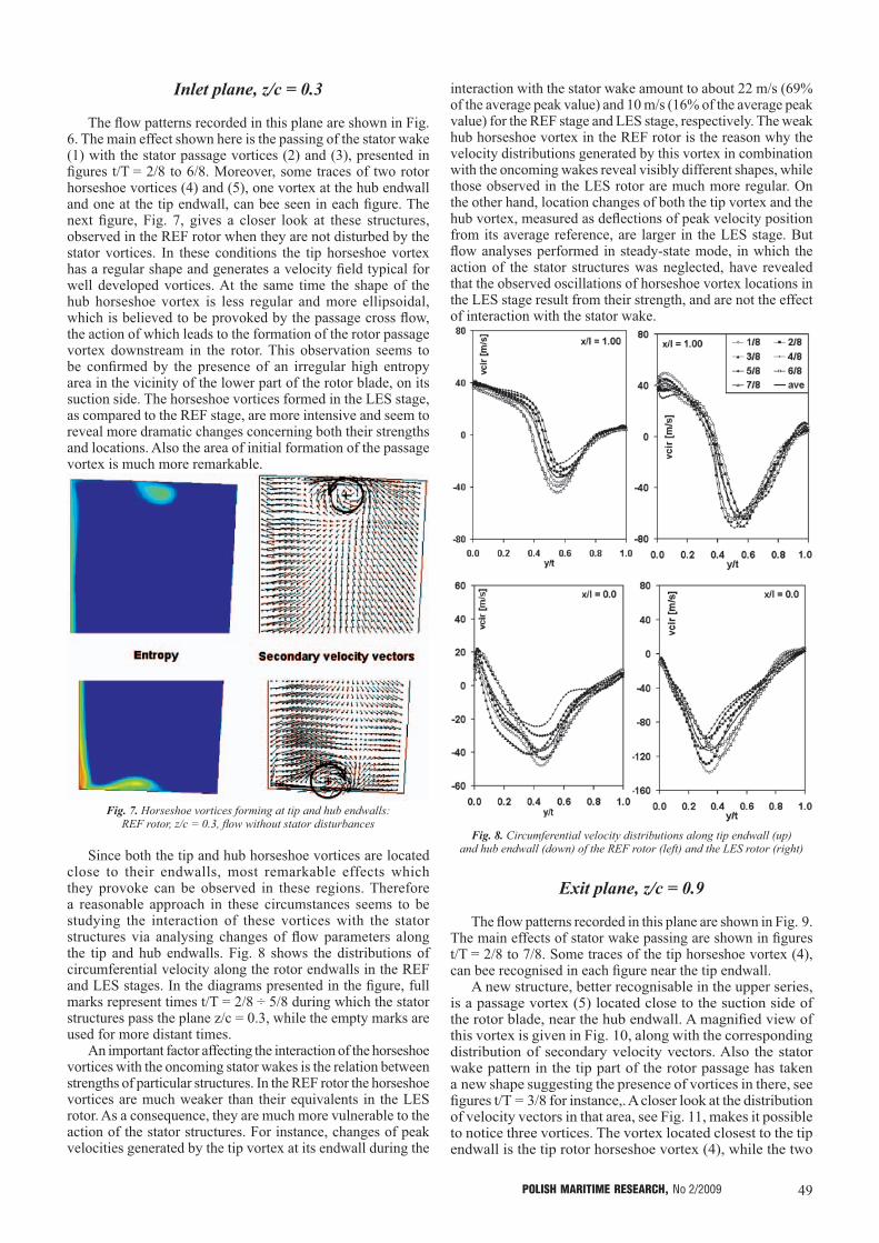
49POLISH MARITIME RESEARCH, No 2/2009
Inlet plane, z/c = 0.3
The flow patterns recorded in this plane are shown in Fig. 6. The main effect shown here is the passing of the stator wake (1) with the stator passage vortices (2) and (3), presented in figures t/T = 2/8 to 6/8. Moreover, some traces of two rotor horseshoe vortices (4) and (5), one vortex at the hub endwall and one at the tip endwall, can bee seen in each figure. The next figure, Fig. 7, gives a closer look at these structures, observed in the REF rotor when they are not disturbed by the stator vortices. In these conditions the tip horseshoe vortex has a regular shape and generates a velocity field typical for well developed vortices. At the same time the shape of the hub horseshoe vortex is less regular and more ellipsoidal, which is believed to be provoked by the passage cross flow, the action of which leads to the formation of the rotor passage vortex downstream in the rotor. This observation seems to be confirmed by the presence of an irregular high entropy area in the vicinity of the lower part of the rotor blade, on its suction side. The horseshoe vortices formed in the LES stage, as compared to the REF stage, are more intensive and seem to reveal more dramatic changes concerning both their strengths and locations. Also the area of initial formation of the passage vortex is much more remarkable.
Fig. 7. Horseshoe vortices forming at tip and hub endwalls: REF rotor, z/c = 0.3, flow without stator disturbances
Since both the tip and hub horseshoe vortices are located close to their endwalls, most remarkable effects which they provoke can be observed in these regions. Therefore a reasonable approach in these circumstances seems to be studying the interaction of these vortices with the stator structures via analysing changes of flow parameters along the tip and hub endwalls. Fig. 8 shows the distributions of circumferential velocity along the rotor endwalls in the REF and LES stages. In the diagrams presented in the figure, full marks represent times t/T = 2/8 ÷ 5/8 during which the stator structures pass the plane z/c = 0.3, while the empty marks are used for more distant times.
An important factor affecting the interaction of the horseshoe vortices with the oncoming stator wakes is the relation between strengths of particular structures. In the REF rotor the horseshoe vortices are much weaker than their equivalents in the LES rotor. As a consequence, they are much more vulnerable to the action of the stator structures. For instance, changes of peak velocities generated by the tip vortex at its endwall during the
interaction with the stator wake amount to about 22 m/s (69% of the average peak value) and 10 m/s (16% of the average peak value) for the REF stage and LES stage, respectively. The weak hub horseshoe vortex in the REF rotor is the reason why the velocity distributions generated by this vortex in combination with the oncoming wakes reveal visibly different shapes, while those observed in the LES rotor are much more regular. On the other hand, location changes of both the tip vortex and the hub vortex, measured as deflections of peak velocity position from its average reference, are larger in the LES stage. But flow analyses performed in steady-state mode, in which the action of the stator structures was neglected, have revealed that the observed oscillations of horseshoe vortex locations in the LES stage result from their strength, and are not the effect of interaction with the stator wake.
Fig. 8. Circumferential velocity distributions along tip endwall (up) and hub endwall (down) of the REF rotor (left) and the LES rotor (right)
Exit plane, z/c = 0.9
The flow patterns recorded in this plane are shown in Fig. 9. The main effects of stator wake passing are shown in figures t/T = 2/8 to 7/8. Some traces of the tip horseshoe vortex (4), can bee recognised in each figure near the tip endwall.
A new structure, better recognisable in the upper series, is a passage vortex (5) located close to the suction side of the rotor blade, near the hub endwall. A magnified view of this vortex is given in Fig. 10, along with the corresponding distribution of secondary velocity vectors. Also the stator wake pattern in the tip part of the rotor passage has taken a new shape suggesting the presence of vortices in there, see figures t/T = 3/8 for instance,. A closer look at the distribution of velocity vectors in that area, see Fig. 11, makes it possible to notice three vortices. The vortex located closest to the tip endwall is the tip rotor horseshoe vortex (4), while the two

50 POLISH MARITIME RESEARCH, No 2/2009
remaining vortices are stator structures. Based on the analysis presented by Doerffer et al. [11], they can be recognised as the stator passage vortex (2), of clockwise rotation, and the so-called trailing shed vortex (6), of counterclockwise rotation, which forms due to the interaction of the stator passage vortex with the stator blade trailing edge. It is noteworthy that making distinction between those two structures earlier, in rotor passage sections located upstream of z/c = 0.9, was very difficult due to low strength of the stator passage vortex.
Fig. 11. Combination of vortices near rotor passage tip endwall: REF stage, z/c = 0.9, flow at presence of stator wake
The interaction of the vortex structures in the LES rotor is much more unstable than in the REF rotor. This is especially noticeable for the rotor passage vortex (5) which in some figures breaks down into two structures. A detailed study of this phenomenon in classical steady-state conditions, when the effect of stator/rotor interaction is neglected, has revealed that in this case the process of passage vortex formation is highly unsteady and takes a cyclic course, Fig. 12, during which the
Fig. 9. Flow patterns in exit rotor passage plane, z/c = 0.9: top - REF stage, bottom - LES stage
Fig. 10. Rotor passage vortex near rotor blade suction side: REF stage, z/c = 0.9, flow without stator disturbances
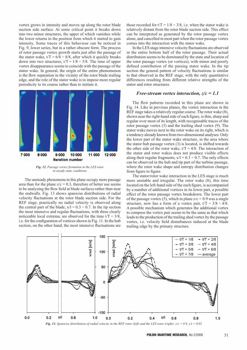
51POLISH MARITIME RESEARCH, No 2/2009
vortex grows in intensity and moves up along the rotor blade suction side surface. At some critical point it breaks down into two minor structures, the upper of which vanishes while the lower returns to the position from which it started to gain intensity. Some traces of this behaviour can be noticed in Fig. 9, lower series, but in a rather obscure form. The process of rotor passage vortex growth starts just after the passage of the stator wake, t/T = 6/8 ÷ 8/8, after which it quickly breaks down into two structures, t/T = 1/8 ÷ 3/8. The time of upper vortex disappearance seems to coincide with the passage of the stator wake. In general, the origin of the entire phenomenon is the flow separation in the vicinity of the rotor blade trailing edge, and the role of the stator wake is to impose more regular periodicity to its course rather than to initiate it.
Fig. 12. Passage vortex formation in the LES rotor in steady-state conditions
The unsteady phenomena in this plane occupy more passage area than for the plane z/c = 0.3, therefore of better use seems to be analysing the flow field at blade surfaces rather than near the endwalls. Fig. 13 shows spanwise distributions of radial velocity fluctuations at the rotor blade suction side. For the REF stage, practically no radial velocity is observed along the central part of the blade, x/l = 0.3 ÷ 0.7. In the tip section the most intensive and regular fluctuations, with three clearly noticeable local extrema, are observed for the time t/T = 3/8, i.e. for the configuration of vortices shown in Fig. 11. In the hub section, on the other hand, the most intensive fluctuations are
those recorded for t/T = 1/8 ÷ 3/8, i.e. when the stator wake is relatively distant from the rotor blade suction side. This effect can be interpreted as generated by the rotor passage vortex alone, and cancelled in most part when the rotor passage vortex comes into the interaction with the stator wake.
In the LES stage intensive velocity fluctuations are observed in the entire bottom half of the rotor passage. Their actual distribution seems to be dominated by the state and location of the rotor passage vortex (or vortices), with minor and poorly defined contribution of the passing stator wake. In the tip section the general pattern of velocity fluctuations is similar to that observed in the REF stage, with the only quantitative differences resulting from different relative strengths of the stator and rotor structures.
Free-stream vortex interaction, z/c = 1.1
The flow patterns recorded in this plane are shown in Fig. 14. Like in previous planes, the vortex interaction in the REF stage takes a relatively regular course. The rotor wake (8), shown near the right-hand side of each figure, is thin, sharp and regular over most of its length, with recognisable traces of the rotor passage vortex (5) and the trailing shed vortex (9). The stator wake moves next to the rotor wake on its right, which is a tendency already known from two-dimensional analyses. Only the lower part of the stator wake structure, in the area where the stator hub passage vortex (3) is located, is shifted towards the other side of the rotor wake, t/T = 4/8. The interaction of the stator and rotor wakes does not produce visible effects along their regular fragments, x/l = 0.3 ÷ 0.7. The only effects can be observed in the hub and tip part of the turbine passage, where the rotor wake shape and entropy distribution changes from figure to figure.
The stator/rotor wake interaction in the LES stage is much more unstable and irregular. The rotor wake (8), this time located on the left-hand side of the each figure, is accompanied by a number of additional vortices in its lower part, a possible effect of the rotor passage vortex breakdown. The lower part of the passage vortex (5), which in plane z/c = 0.9 was a single structure, now has a form of a vortex pair, t/T = 3/8 ÷ 4/8. A possible mechanism which generates the additional vortex to compose the vortex pair seems to be the same as that which leads to the production of the trailing shed vortex by the passage vortex, i.e. velocity field disturbances induced at the blade trailing edge by the primary structure.
Fig. 13. Spanwise distribution of radial velocity in the REF rotor (left) and the LES rotor (right): z/c = 0.9, y/t = 0.02

52 POLISH MARITIME RESEARCH, No 2/2009
Fig. 14. Free-stream vortex interaction downstream of the rotor, z/c = 1.1: top - REF stage, bottom - LES stage
Fig. 15. Absolute flow angles at rotor exit, z/c = 1.1: top – REF stage, bottom - LES stage

53POLISH MARITIME RESEARCH, No 2/2009
The measurable effects of vortex interaction in the examined plane are shown in Fig. 15, in the form of distributions of absolute flow angles (measured from the axial direction) in selected traverses x/l = const. Thin curves in the figure represent individual realisations, while the thick one is their average. In the upper series, for the REF stage, the effect of the stator/rotor wake interaction can be observed as: (a) changes in the intensity and location of the peak on the right, which represents the rotor wake, and (b) flow angle fluctuations observed close to the left-hand part of the diagram and provoked directly by the passing stator wake. Both types of disturbances are the highest for the extreme x/l values: x/l = 0.18 and 0.95, but even in those cases they do not diverge by more that 25 degrees from corresponding average local values. In the LES stage flow angle fluctuations are much more intensive and irregular, and in extreme cases can reach over 70 degrees, x/l = 0.25, y/t = 0.4.
CONCLUSIONS
� The paper presents an analysis of the three-dimensional interaction of vortex structures in a turbine rotor. Two high-pressure steam turbine stages were selected as representative for the examination: the standard (REF) stage which revealed regular performance characteristics and distributions of flow parameters, and the low-efficiency (LES) stage in which a separation zone was observed in the rear part of the rotor passage. In the REF rotor the passing stator structures provoke noticeable changes in instantaneous strengths and locations of the horseshoe and passage vortices forming in the rotor passage area. In the LES stage, on the other hand, where the rotor vortices are much more intensive and unstable, they are the main source of flow unsteadiness, only slightly affected by the passing stator wakes the role of which is to in to introduce some regularity in the development of the rotor structures.
� The information on the presented two interaction patterns contributes to better understanding of unsteady phenomena taking place in turbine rotors, and is believed to be applicable for a variety of turbine stage constructions with radial blades. In large stationary turbine stages, with well designed profiles and optimised stage operation conditions, the pattern referred to as REF in the article is believed to be representative for the vortex interaction. At the same time for smaller turbines of both land and marine applications, where certain technological limitations make it impossible for the stage design to follow all flow requirements and the
resultant stage operation efficiency is relatively low, the vortex interaction pattern close to that here referred to as LES is likely to be observed.
BIBLIOGRAPHY
1. Goldstein R.J., Spores R.A.: Turbulent transport on the endwall in the region between adjacent turbine blades, Trans. ASME, J. Heat Transfer, vol. 110, 1988
2. Doerffer P., Amecke J.: Secondary flow control and stream-wise vortices formation, ASME Paper. 94-GT-376, 1994
3. Wang H.P., Olson S.J., Goldstein R.J., Eckert E.R.G.: Flow visualization of a linear turbine cascade of high performance turbine blades, J. Fluid Mech., vol. 134, 1997
4. Swirydczuk J.: Grid resolution in numeric analyses of stator/rotor interactions (in Polish), SYSTEMS Journal of Transdisciplinary Systems Science, vol. 11, 2006
5. Lardeau, S., Leschziner, M.A. : Unsteady RANS modelling of wake-blade interaction: computational requirements and limitations”, Computers & Fluids, vol. 34, 2005
6. Yershov, S., Rusanov, A., Gardzilewicz, A., Lampart, P., Swirydczuk, J.: Numerical Simulation of 3D Flow in Axial Turbomachines, TASK Quarterly, vol. 2, 1998
7. Lampart P. , Swirydczuk J., Gardzilewicz A.: On the prediction of flow patterns and losses in an HP axial turbine stages using 3D RANS solver with two turbulence models, TASK Quarterly vol. 5, 2001
8. Lampart P., Rusanov A., Yershov S., Marcinkowski S., Gardzilewicz A.: Validation of a 3D RANS Solver With a State Equation of Thermally Perfect and Calorically Imperfect Gas on a Multi-Stage Low-Pressure Steam Turbine Flow, ASME J. Fluids Engineering, vol. 127, 2005
9. Swirydczuk J.: Vortex Dynamics of the Stator Wake-Rotor Cascade Interaction, ASME J. Fluids Engineering, vol. 124, 2002
10. Kost F., Hummel F., Tiedemann M.: Investigation of the Unsteady Rotor Flow Field in a Single HP Turbine Stage, Proc. ASME TURBO EXPO 2000, May 8-11, Munich, Germany, 2000
11. Doerffer P., Rachwalski J., Magagnato F.: Numerical Investigation of the Secondary Flow Development in Turbine Cascade, TASK Quarterly, vol. 5, 2001.
CONTACT WITH THE AUTHOR
Jerzy Świrydczuk, Assoc. Prof.Institute of Fluid-Flow Machinery
Fiszera 1480-952 Gdansk, POLAND
e-mail: [email protected]

54 POLISH MARITIME RESEARCH, No 2/2009
INTRODUCTION
A ship is a complex technical object in which the principles of propagation of acoustic signals are complicated. Therefore minimising the propagation of internal noise is a difficult task, due to specific conditions taking place on floating objects of this type. The hull is a separate structure inside which numerous sources of strong noise are located. This is especially true for the engine room, limited in space, in which the access is to be secured to the main engine, gear, propeller shaft and auxiliary units, such as electric current generator, pumps, fans, etc. These limitations make potential use of some methods to minimise vibroacoustic effects accompanying the operation of the above devices extremely difficult. Of high importance in ship nose fighting is the identification of both the sources and propagation paths of the vibroacoustic energy acting in a direct way, or having the form of reflection and/or diffraction waves, which generate sound in the air and materials.
The main source of vibroacoustic signals on a ship are internal combustion engines, i.e. the main engine and auxiliary engines driving, for instance, electric current generators. Other sources of remarkable vibrations of this type include auxiliary devices such as pumps, compressors, hydraulic systems, main engine gears, propellers, and air conditioning and ventilation systems. The contribution of particular sources in the total level of noise in the engine room depends on their location inside the hull and the type and dimensions of the ship. These sources are most frequently located in the after body, from which they act
on the living and working ship compartments. The dominating sounds in the engine room compartment are the air sounds – direct and reflected. In a larger distance from the source, the dominating effects in the noise are material sounds.
Due to mechanical power transmission, the vibrating main engine, excited by the action of varying forces, is the main source of the acoustic energy of both the air and material type. The exciting forces come from:� pressure pulsations in the inlet and outlet ducts� pressure changes in cylinders during the combustion
process� operation of the timing gear� pressure changes in fuel and lubrication systems� inertia of moving engine elements� toothed gears� auxiliary devices.
Frequencies of these forces are connected with the rotational speed of the engine crankshaft, and are defined as [2, 3]:
(1)
where:n – rotational speed of the crankshaft
[rev/min]ZC – number of cylinderss = 2 – for four-stroke enginesk = 0,5; 1; 2; 3… – harmonics of the exciting forces.
Janusz Gardulski, Assoc. Prof.Silesian University of Technology
Vibration and noise minimisation in living and working ship compartments
ABSTRACT
The article discusses the problem of minimisation of the noise emitted by mechanical devices installed on a ship to its living and working compartments. Basic features of the abovementioned mechanical systems are defined taking into account frequencies generated by them. Passive and active methods of noise minimisation via interference into the propagation path are presented. In the conclusion, expected effects
are formulated.
Key words: vibroacoustic signals generated by mechanical devices on a ship; minimisation of vibroacoustic signals
POLISH MARITIME RESEARCH 2(60) 2009 Vol 16; pp. 54-5910.2478/v10012-008-0022-8
55POLISH MARITIME RESEARCH, No 2/2009
After defining the rotational frequency caused by the unbalance of the rotating masses as:
(2)
we get the frequencies connected with the operation of the engine sub-assemblies:� camshaft frequency
(3)
where:i – camshaft drive transmission ratio (i = 0,5).
� valve closing frequency
(4)
where:ZZ – number of separately working valves.
� toothed gear frequency
(5)
where:z – number of pinion teeth.
� fan blade frequency
(6)
where:l – number of blades.
Like for fans, the frequencies of the impeller pumps are connected with the number of pump blades l and the frequency f’n of the driving motor revolutions.
(7)
The frequency of the electric current generators is most frequently equal to 50 [Hz].
It results from the above relations that different engine sub-assemblies generate the same frequencies, in particular when the energy spectrum reveals harmonic frequencies of the exciting forces caused by nonlinearities of the mechanical systems.
The above list of exciting sources includes low-frequency sources, below 100 [Hz] (main engine with the exhaust system and generators) and high-frequency forces, above 1 kHz (fans, pumps, tooted gears, etc.) This makes using any general method to minimise the vibrations and noise generated by those devices very difficult.
The level of the acoustic pressure generated by the engines used on ships can be approximately calculated from the relation [2]:
(8)
where:N – engine power [kW]n – rotational speed of the crankshaft [rev/min].
This level depends on a number of design factors, such as, for instance, geometrical dimensions of the pistons, type of hull material, etc.
The level of the acoustic power of the low- and medium-power Diesel engines is approximately equal to [2]
(9)
where: NZ corresponds to the nominal engine power [kW] recorded at its nominal rotational speed nZ [rev/min].
Major part of the acoustic energy is transmitted from the engine via a material path. The vibrations are transmitted to the elements of the steel hull structure not only through the foundations, but also trough the propeller shaft, engine fittings, fuel, lubrication and cooling systems, and other auxiliary devices. Low-speed engines working with rotational speed ranging between 100 and 250 rev/min emit vibroacoustic signals ranging from a few to about 200 Hz, while the medium-speed engines (n = 350 – 1000 rev/min) cooperating with the toothed gear – up to 2000 Hz. Moreover, these engines, when cooperating with a gear, reach the sound level higher by up to 15 dB than that recorded for the low-speed engines [6].
The origin of the acoustic effects generated during the operation of the ship propeller is turbulence and cavitation, which both appear on the edges of the propeller when the circumferential velocities are sufficiently high. The cavitation noise spectrum is within the frequency limits of 20 – 500 Hz. The turbulence and the cavitation act on the ship hull and make it vibrate. The excited large-area plate panels become secondary sources of the broadband noise of large acoustic power.
MINIMISATION OF THE LEVEL OF NOISE AND VIBRATIONS GENERATED IN THE
ENGINE ROOM
The vibroacoustic signals emitted by the driving system can be minimised by:� changes of aerodynamic coefficients at device’s inlet and
outlet and inside its working space,� minimisation of the exciting forces and their spectra.
Changes of the aerodynamic conditions can be obtained by the use of covers, to damp the vibrations, and silencers at inlets and outlets of the main and auxiliary engines, while the exciting forces can be minimised using vibration absorbers.
Minimisation of the vibration level
Damping is connected with the dissipation of the mechanical energy converted, for instance, to the thermal energy, i.e. with decreasing the general efficiency of device’s operation. That is why the damping is only introduced when the minimisation cannot be obtained via structural and parametrical modifications. Such an approach accompanies active methods, unlike those based on changes of the transmission path – by introducing vibroinsulation. Three groups of methods of structure modification can be named. The first method consists in introducing additional internal connections to the system using elastic absorbing elements (disc connections, for instance). In the second method, additional masses (Frame type, for instance) are introduced to the object, while in the third method the required effect is obtained by rearranging the structure continuity using intermediate flexible elements (vibroinsulators).
The main disadvantage of the dynamic vibration eliminators is that they can only be used for harmonic excitations (they are tuned to a precisely defined frequency). They do not bring profits in the mechanical systems used in unsteady conditions. Similar disadvantages are revealed by the parametric modification of a mechanical system in which the parameters are the load vector variables: inertia „M”, stiffness „K” and damping „C” of the system. During its operation a real nonlinear mechanical system is subject to the action of an exciting force having a broad spectrum and large number of harmonics. In order to reduce the amplitude of the vibrations, broad-spectrum exciting forces are to be decreased.
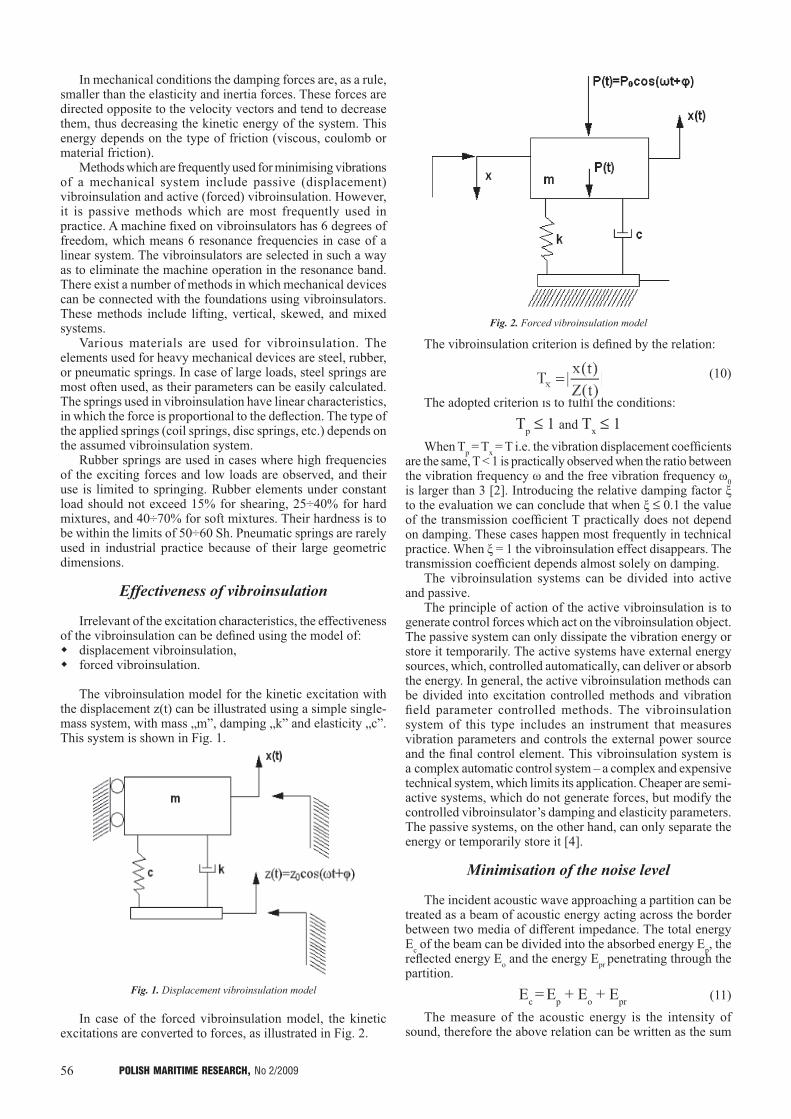
56 POLISH MARITIME RESEARCH, No 2/2009
In mechanical conditions the damping forces are, as a rule, smaller than the elasticity and inertia forces. These forces are directed opposite to the velocity vectors and tend to decrease them, thus decreasing the kinetic energy of the system. This energy depends on the type of friction (viscous, coulomb or material friction).
Methods which are frequently used for minimising vibrations of a mechanical system include passive (displacement) vibroinsulation and active (forced) vibroinsulation. However, it is passive methods which are most frequently used in practice. A machine fixed on vibroinsulators has 6 degrees of freedom, which means 6 resonance frequencies in case of a linear system. The vibroinsulators are selected in such a way as to eliminate the machine operation in the resonance band. There exist a number of methods in which mechanical devices can be connected with the foundations using vibroinsulators. These methods include lifting, vertical, skewed, and mixed systems.
Various materials are used for vibroinsulation. The elements used for heavy mechanical devices are steel, rubber, or pneumatic springs. In case of large loads, steel springs are most often used, as their parameters can be easily calculated. The springs used in vibroinsulation have linear characteristics, in which the force is proportional to the deflection. The type of the applied springs (coil springs, disc springs, etc.) depends on the assumed vibroinsulation system.
Rubber springs are used in cases where high frequencies of the exciting forces and low loads are observed, and their use is limited to springing. Rubber elements under constant load should not exceed 15% for shearing, 25÷40% for hard mixtures, and 40÷70% for soft mixtures. Their hardness is to be within the limits of 50÷60 Sh. Pneumatic springs are rarely used in industrial practice because of their large geometric dimensions.
Effectiveness of vibroinsulation
Irrelevant of the excitation characteristics, the effectiveness of the vibroinsulation can be defined using the model of: displacement vibroinsulation, forced vibroinsulation.
The vibroinsulation model for the kinetic excitation with the displacement z(t) can be illustrated using a simple single-mass system, with mass „m”, damping „k” and elasticity „c”. This system is shown in Fig. 1.
Fig. 1. Displacement vibroinsulation model
In case of the forced vibroinsulation model, the kinetic excitations are converted to forces, as illustrated in Fig. 2.
Fig. 2. Forced vibroinsulation model
The vibroinsulation criterion is defined by the relation:
(10)
The adopted criterion is to fulfil the conditions:
Tp ≤ 1 and Tx ≤ 1When Tp = Tx = T i.e. the vibration displacement coefficients
are the same, T < 1 is practically observed when the ratio between the vibration frequency ω and the free vibration frequency ω0 is larger than 3 [2]. Introducing the relative damping factor ξ to the evaluation we can conclude that when ξ ≤ 0.1 the value of the transmission coefficient T practically does not depend on damping. These cases happen most frequently in technical practice. When ξ = 1 the vibroinsulation effect disappears. The transmission coefficient depends almost solely on damping.
The vibroinsulation systems can be divided into active and passive.
The principle of action of the active vibroinsulation is to generate control forces which act on the vibroinsulation object. The passive system can only dissipate the vibration energy or store it temporarily. The active systems have external energy sources, which, controlled automatically, can deliver or absorb the energy. In general, the active vibroinsulation methods can be divided into excitation controlled methods and vibration field parameter controlled methods. The vibroinsulation system of this type includes an instrument that measures vibration parameters and controls the external power source and the final control element. This vibroinsulation system is a complex automatic control system – a complex and expensive technical system, which limits its application. Cheaper are semi-active systems, which do not generate forces, but modify the controlled vibroinsulator’s damping and elasticity parameters. The passive systems, on the other hand, can only separate the energy or temporarily store it [4].
Minimisation of the noise level
The incident acoustic wave approaching a partition can be treated as a beam of acoustic energy acting across the border between two media of different impedance. The total energy Ec of the beam can be divided into the absorbed energy Ep, the reflected energy Eo and the energy Epr penetrating through the partition.
Ec = Ep + Eo + Epr (11)
The measure of the acoustic energy is the intensity of sound, therefore the above relation can be written as the sum
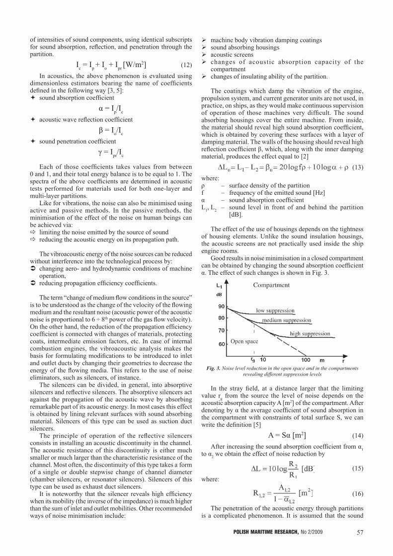
57POLISH MARITIME RESEARCH, No 2/2009
of intensities of sound components, using identical subscripts for sound absorption, reflection, and penetration through the partition.
Ic = Ip + Io + Ipr [W/m2] (12)
In acoustics, the above phenomenon is evaluated using dimensionless estimators bearing the name of coefficients defined in the following way [3, 5]:� sound absorption coefficient
α = Ip/Ic
� acoustic wave reflection coefficient
β = Io/Ic
� sound penetration coefficient
γ = Ipr/Ic
Each of those coefficients takes values from between 0 and 1, and their total energy balance is to be equal to 1. The spectra of the above coefficients are determined in acoustic tests performed for materials used for both one-layer and multi-layer partitions.
Like for vibrations, the noise can also be minimised using active and passive methods. In the passive methods, the minimisation of the effect of the noise on human beings can be achieved via:� limiting the noise emitted by the source of sound� reducing the acoustic energy on its propagation path.
The vibroacoustic energy of the noise sources can be reduced without interference into the technological process by:� changing aero- and hydrodynamic conditions of machine
operation, � reducing propagation efficiency coefficients.
The term “change of medium flow conditions in the source” is to be understood as the change of the velocity of the flowing medium and the resultant noise (acoustic power of the acoustic noise is proportional to 6 ÷ 8th power of the gas flow velocity). On the other hand, the reduction of the propagation efficiency coefficient is connected with changes of materials, protecting coats, intermediate emission factors, etc. In case of internal combustion engines, the vibroacoustic analysis makes the basis for formulating modifications to be introduced to inlet and outlet ducts by changing their geometries to decrease the energy of the flowing media. This refers to the use of noise eliminators, such as silencers, of instance.
The silencers can be divided, in general, into absorptive silencers and reflective silencers. The absorptive silencers act against the propagation of the acoustic wave by absorbing remarkable part of its acoustic energy. In most cases this effect is obtained by lining relevant surfaces with sound absorbing material. Silencers of this type can be used as suction duct silencers.
The principle of operation of the reflective silencers consists in installing an acoustic discontinuity in the channel. The acoustic resistance of this discontinuity is either much smaller or much larger than the characteristic resistance of the channel. Most often, the discontinuity of this type takes a form of a single or double stepwise change of channel diameter (chamber silencers, or resonator silencers). Silencers of this type can be used as exhaust duct silencers.
It is noteworthy that the silencer reveals high efficiency when its mobility (the inverse of the impedance) is much higher than the sum of inlet and outlet mobilities. Other recommended ways of noise minimisation include:
� machine body vibration damping coatings� sound absorbing housings� acoustic screens� changes of acoustic absorption capacity of the
compartment� changes of insulating ability of the partition.
The coatings which damp the vibration of the engine, propulsion system, and current generator units are not used, in practice, on ships, as they would make continuous supervision of operation of those machines very difficult. The sound absorbing housings cover the entire machine. From inside, the material should reveal high sound absorption coefficient, which is obtained by covering these surfaces with a layer of damping material. The walls of the housing should reveal high reflection coefficient β, which, along with the inner damping material, produces the effect equal to [2]
(13)
where: ρ – surface density of the partitionf – frequency of the emitted sound [Hz]α – sound absorption coefficientL1, L2 – sound level in front of and behind the partition
[dB].
The effect of the use of housings depends on the tightness of housing elements. Unlike the sound insulation housings, the acoustic screens are not practically used inside the ship engine rooms.
Good results in noise minimisation in a closed compartment can be obtained by changing the sound absorption coefficient α. The effect of such changes is shown in Fig. 3.
Fig. 3. Noise level reduction in the open space and in the compartments revealing different suppression levels
In the stray field, at a distance larger that the limiting value rg from the source the level of noise depends on the acoustic absorption capacity A [m2] of the compartment. After denoting by α the average coefficient of sound absorption in the compartment with constraints of total surface S, we can write the definition [5]
A = Sα [m2] (14)
After increasing the sound absorption coefficient from α1 to α2 we obtain the effect of noise reduction by
(15)
where:
(16)
The penetration of the acoustic energy through partitions is a complicated phenomenon. It is assumed that the sound
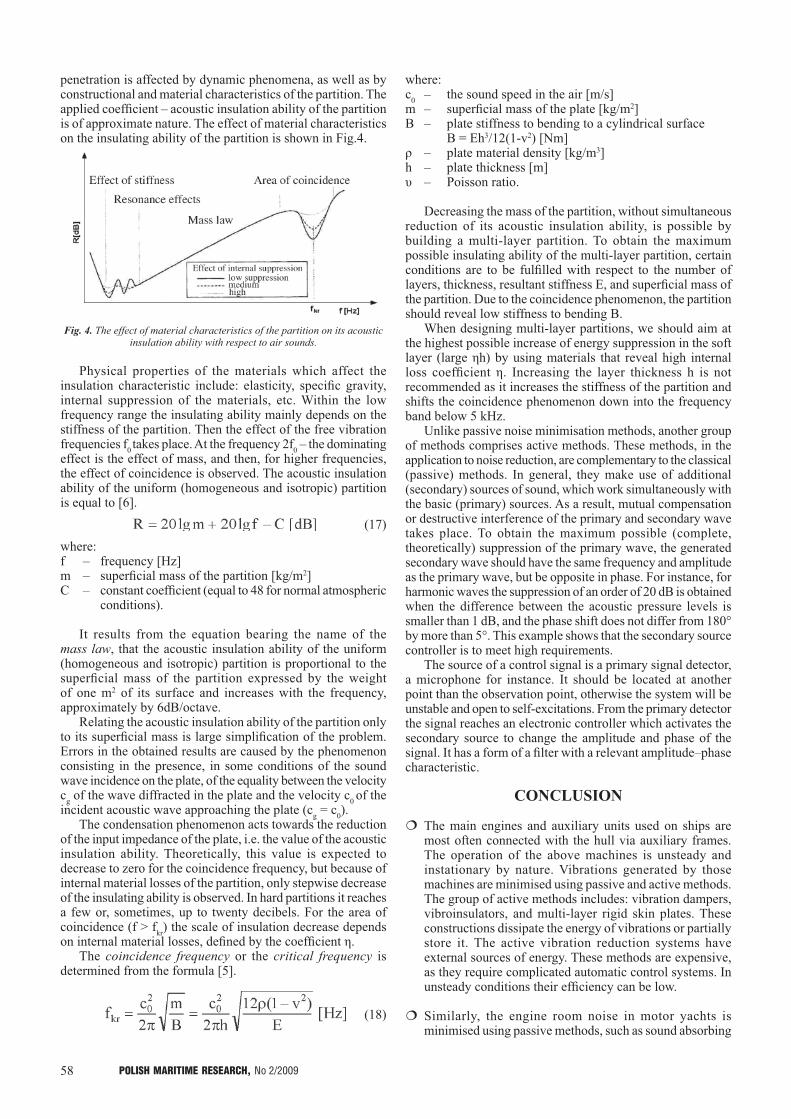
58 POLISH MARITIME RESEARCH, No 2/2009
penetration is affected by dynamic phenomena, as well as by constructional and material characteristics of the partition. The applied coefficient – acoustic insulation ability of the partition is of approximate nature. The effect of material characteristics on the insulating ability of the partition is shown in Fig.4.
Fig. 4. The effect of material characteristics of the partition on its acoustic insulation ability with respect to air sounds.
Physical properties of the materials which affect the insulation characteristic include: elasticity, specific gravity, internal suppression of the materials, etc. Within the low frequency range the insulating ability mainly depends on the stiffness of the partition. Then the effect of the free vibration frequencies f0 takes place. At the frequency 2f0 – the dominating effect is the effect of mass, and then, for higher frequencies, the effect of coincidence is observed. The acoustic insulation ability of the uniform (homogeneous and isotropic) partition is equal to [6].
(17)
where:f – frequency [Hz]m – superficial mass of the partition [kg/m2]C – constant coefficient (equal to 48 for normal atmospheric
conditions).
It results from the equation bearing the name of the mass law, that the acoustic insulation ability of the uniform (homogeneous and isotropic) partition is proportional to the superficial mass of the partition expressed by the weight of one m2 of its surface and increases with the frequency, approximately by 6dB/octave.
Relating the acoustic insulation ability of the partition only to its superficial mass is large simplification of the problem. Errors in the obtained results are caused by the phenomenon consisting in the presence, in some conditions of the sound wave incidence on the plate, of the equality between the velocity cg of the wave diffracted in the plate and the velocity c0 of the incident acoustic wave approaching the plate (cg = c0).
The condensation phenomenon acts towards the reduction of the input impedance of the plate, i.e. the value of the acoustic insulation ability. Theoretically, this value is expected to decrease to zero for the coincidence frequency, but because of internal material losses of the partition, only stepwise decrease of the insulating ability is observed. In hard partitions it reaches a few or, sometimes, up to twenty decibels. For the area of coincidence (f > fkr) the scale of insulation decrease depends on internal material losses, defined by the coefficient η.
The coincidence frequency or the critical frequency is determined from the formula [5].
(18)
where:c0 – the sound speed in the air [m/s]m – superficial mass of the plate [kg/m2]B – plate stiffness to bending to a cylindrical surface B = Eh3/12(1-v2) [Nm]ρ – plate material density [kg/m3]h – plate thickness [m]υ – Poisson ratio.
Decreasing the mass of the partition, without simultaneous reduction of its acoustic insulation ability, is possible by building a multi-layer partition. To obtain the maximum possible insulating ability of the multi-layer partition, certain conditions are to be fulfilled with respect to the number of layers, thickness, resultant stiffness E, and superficial mass of the partition. Due to the coincidence phenomenon, the partition should reveal low stiffness to bending B.
When designing multi-layer partitions, we should aim at the highest possible increase of energy suppression in the soft layer (large ηh) by using materials that reveal high internal loss coefficient η. Increasing the layer thickness h is not recommended as it increases the stiffness of the partition and shifts the coincidence phenomenon down into the frequency band below 5 kHz.
Unlike passive noise minimisation methods, another group of methods comprises active methods. These methods, in the application to noise reduction, are complementary to the classical (passive) methods. In general, they make use of additional (secondary) sources of sound, which work simultaneously with the basic (primary) sources. As a result, mutual compensation or destructive interference of the primary and secondary wave takes place. To obtain the maximum possible (complete, theoretically) suppression of the primary wave, the generated secondary wave should have the same frequency and amplitude as the primary wave, but be opposite in phase. For instance, for harmonic waves the suppression of an order of 20 dB is obtained when the difference between the acoustic pressure levels is smaller than 1 dB, and the phase shift does not differ from 180° by more than 5°. This example shows that the secondary source controller is to meet high requirements.
The source of a control signal is a primary signal detector, a microphone for instance. It should be located at another point than the observation point, otherwise the system will be unstable and open to self-excitations. From the primary detector the signal reaches an electronic controller which activates the secondary source to change the amplitude and phase of the signal. It has a form of a filter with a relevant amplitude–phase characteristic.
CONCLUSION
� The main engines and auxiliary units used on ships are most often connected with the hull via auxiliary frames. The operation of the above machines is unsteady and instationary by nature. Vibrations generated by those machines are minimised using passive and active methods. The group of active methods includes: vibration dampers, vibroinsulators, and multi-layer rigid skin plates. These constructions dissipate the energy of vibrations or partially store it. The active vibration reduction systems have external sources of energy. These methods are expensive, as they require complicated automatic control systems. In unsteady conditions their efficiency can be low.
� Similarly, the engine room noise in motor yachts is minimised using passive methods, such as sound absorbing
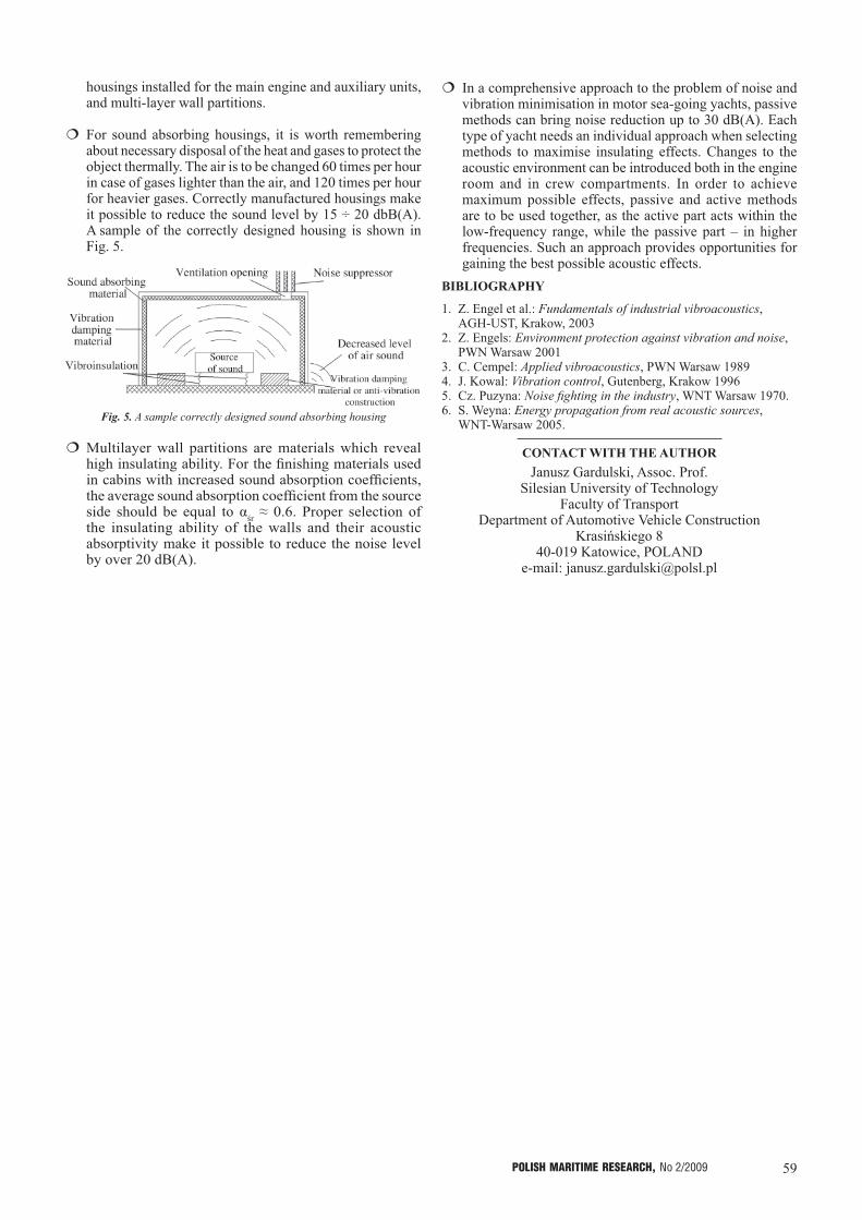
59POLISH MARITIME RESEARCH, No 2/2009
housings installed for the main engine and auxiliary units, and multi-layer wall partitions.
� For sound absorbing housings, it is worth remembering about necessary disposal of the heat and gases to protect the object thermally. The air is to be changed 60 times per hour in case of gases lighter than the air, and 120 times per hour for heavier gases. Correctly manufactured housings make it possible to reduce the sound level by 15 ÷ 20 dbB(A). A sample of the correctly designed housing is shown in Fig. 5.
Fig. 5. A sample correctly designed sound absorbing housing
� Multilayer wall partitions are materials which reveal high insulating ability. For the finishing materials used in cabins with increased sound absorption coefficients, the average sound absorption coefficient from the source side should be equal to αśr ≈ 0.6. Proper selection of the insulating ability of the walls and their acoustic absorptivity make it possible to reduce the noise level by over 20 dB(A).
� In a comprehensive approach to the problem of noise and vibration minimisation in motor sea-going yachts, passive methods can bring noise reduction up to 30 dB(A). Each type of yacht needs an individual approach when selecting methods to maximise insulating effects. Changes to the acoustic environment can be introduced both in the engine room and in crew compartments. In order to achieve maximum possible effects, passive and active methods are to be used together, as the active part acts within the low-frequency range, while the passive part – in higher frequencies. Such an approach provides opportunities for gaining the best possible acoustic effects.
BIBLIOGRAPHY
1. Z. Engel et al.: Fundamentals of industrial vibroacoustics, AGH-UST, Krakow, 2003
2. Z. Engels: Environment protection against vibration and noise, PWN Warsaw 2001
3. C. Cempel: Applied vibroacoustics, PWN Warsaw 19894. J. Kowal: Vibration control, Gutenberg, Krakow 19965. Cz. Puzyna: Noise fighting in the industry, WNT Warsaw 1970.6. S. Weyna: Energy propagation from real acoustic sources,
WNT-Warsaw 2005.
CONTACT WITH THE AUTHORJanusz Gardulski, Assoc. Prof.
Silesian University of TechnologyFaculty of Transport
Department of Automotive Vehicle Construction Krasińskiego 8
40-019 Katowice, POLANDe-mail: [email protected]

60 POLISH MARITIME RESEARCH, No 2/2009
INTRODUCTION
Chemical compounds of oxygen and nitrogen (NOx) emitted to the atmosphere with the exhaust gas from a ship engine are a source of pollution of the marine environment. In order to prevent negative effects on the environment, the International Marine Organisation adopted Annex VI to the MARPOL 73/78 Convention. This Annex forces the ship owners to reduce the emission of NOx down to the agreed limits defined in the NOx Technical Code [1]. According to these regulations, each ship engine with power exceeding 130 kW is to have a certificate which confirms the compliance of the level of NOx emitted by the engine with the limits in force. Obligatorily, this certificate is to be prolonged after a certain time period, which is done by comparing selected engine parameters which are decisive for NOx emission with the records collected in a technical file specially created for this purpose. Any changes in the engine structure or control system which go beyond the scope defined in the technical file require new measurements performed directly on the ship. Unfortunately, the ship power plant is not equipped, as a rule, with a proper exhaust gas analyser, which makes performing these measurements extremely difficult. Moreover, the measurements of NOx concentration are to be done at precisely defined engine operation points. For the main engine, this means withdrawal of the ship from operation for the time of measurement, a requirement which leads to remarkable increase of operating costs. The regulations of the NOx Technical Code make it possible to use a simplified method of measurement, compared to that used in land applications, which requires the measurements
ANN based evaluation of the NOx concentration in the exhaust gas of a marine two-stroke
diesel engine
at 4 points of engine operation only. This approach, however, results in decreased accuracy of the measurements. That is why Code regulations permit the possibility to exceed the assumed emission limits by 10% in case of measurements performed on an engine supplied with diesel oil, and 15% for an engine supplied with heavy fuel oil.
The above situation is the reason why numerous research centres search for alternative methods for evaluating the level of NOx emitted by an internal combustion engine. Kyrtatos at al. [2] proposed a “software sensor for exhaust emissions estimation” built based on a multi-zone, thermochemical model of NOx production in the cylinder chamber of an engine. This model takes only into account the Zeldowicz mechanism of NOx production [3]. A continuation of this method is a zero-dimensional, thermochemical model proposed by the author of this article [4, 5]. It was worked out based on the Konnov model [6] and includes 724 chemical reactions between 83 compounds taking part in the fuel combustion process in the engine cylinder. The results of the investigations confirm the applicability of the model for evaluating the NOx emission level, but only with respect to a given engine. Extending the model application range requires the implementation of more complicated calculation algorithms, which goes beyond calculating abilities of the computers available on ships. The cost of modelling can be reduced by the use of an Artificial Neural Network (ANN) as a general-purpose approximator of complicated calculation algorithms. The ANN training method proposed by Werbos [7] and bearing the name of the error back propagation method makes it possible to use the ANN in various branches of knowledge. Wang et al. [8], Oladsine
Jerzy Kowalski, Ph.D.Gdynia Maritime University
ABSTRACT
The article presents results of a study on the possible application of artificial neural networks (ANNs) to the evaluation of NOx concentration in the exhaust gas of a marine two-stroke Diesel engine. A concept is presented how to use the ANN as an alternative to direct measurements carried out on a ship at sea. Methods of proper ANN selection, configuration and training are presented. Also included are the results of laboratory tests, performed to obtain data for ANN training and tests, and the results obtained from modelling certain processes with the aid of selected ANNs. As a result of the performed investigations, an ANN was constructed and trained to calculate NOx concentration in the Diesel engine exhaust gas based on the engine operation parameters measured with an average error of 1.83% , and the fuel consumption
measured with an average error of 1.12%.
Keywords: artificial neural network; marine two-stroke engine; NOx concentration; Annex VI to Marpol Convention
POLISH MARITIME RESEARCH 2(60) 2009 Vol 16; pp. 60-6610.2478/v10012-008-0023-7
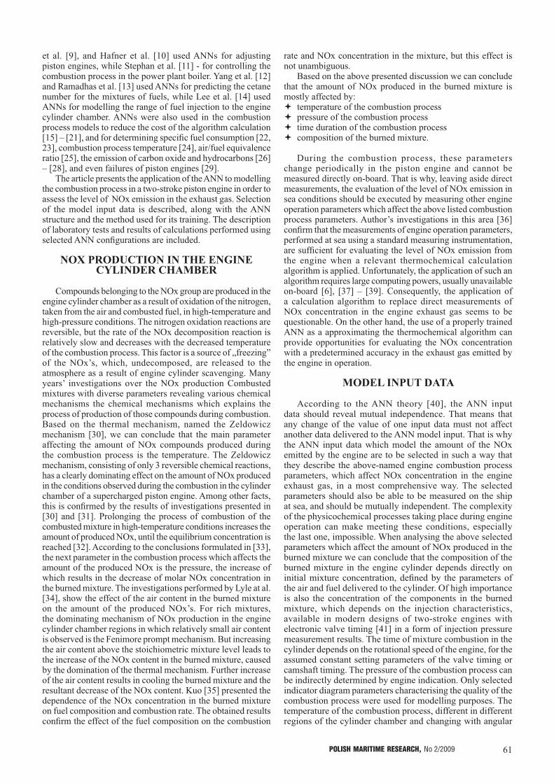
61POLISH MARITIME RESEARCH, No 2/2009
et al. [9], and Hafner et al. [10] used ANNs for adjusting piston engines, while Stephan et al. [11] - for controlling the combustion process in the power plant boiler. Yang et al. [12] and Ramadhas et al. [13] used ANNs for predicting the cetane number for the mixtures of fuels, while Lee et al. [14] used ANNs for modelling the range of fuel injection to the engine cylinder chamber. ANNs were also used in the combustion process models to reduce the cost of the algorithm calculation [15] – [21], and for determining specific fuel consumption [22, 23], combustion process temperature [24], air/fuel equivalence ratio [25], the emission of carbon oxide and hydrocarbons [26] – [28], and even failures of piston engines [29].
The article presents the application of the ANN to modelling the combustion process in a two-stroke piston engine in order to assess the level of NOx emission in the exhaust gas. Selection of the model input data is described, along with the ANN structure and the method used for its training. The description of laboratory tests and results of calculations performed using selected ANN configurations are included.
NOX PRODUCTION IN THE ENGINE CYLINDER CHAMBER
Compounds belonging to the NOx group are produced in the engine cylinder chamber as a result of oxidation of the nitrogen, taken from the air and combusted fuel, in high-temperature and high-pressure conditions. The nitrogen oxidation reactions are reversible, but the rate of the NOx decomposition reaction is relatively slow and decreases with the decreased temperature of the combustion process. This factor is a source of „freezing” of the NOx’s, which, undecomposed, are released to the atmosphere as a result of engine cylinder scavenging. Many years’ investigations over the NOx production Combusted mixtures with diverse parameters revealing various chemical mechanisms the chemical mechanisms which explains the process of production of those compounds during combustion. Based on the thermal mechanism, named the Zeldowicz mechanism [30], we can conclude that the main parameter affecting the amount of NOx compounds produced during the combustion process is the temperature. The Zeldowicz mechanism, consisting of only 3 reversible chemical reactions, has a clearly dominating effect on the amount of NOx produced in the conditions observed during the combustion in the cylinder chamber of a supercharged piston engine. Among other facts, this is confirmed by the results of investigations presented in [30] and [31]. Prolonging the process of combustion of the combusted mixture in high-temperature conditions increases the amount of produced NOx, until the equilibrium concentration is reached [32]. According to the conclusions formulated in [33], the next parameter in the combustion process which affects the amount of the produced NOx is the pressure, the increase of which results in the decrease of molar NOx concentration in the burned mixture. The investigations performed by Lyle at al. [34], show the effect of the air content in the burned mixture on the amount of the produced NOx’s. For rich mixtures, the dominating mechanism of NOx production in the engine cylinder chamber regions in which relatively small air content is observed is the Fenimore prompt mechanism. But increasing the air content above the stoichiometric mixture level leads to the increase of the NOx content in the burned mixture, caused by the domination of the thermal mechanism. Further increase of the air content results in cooling the burned mixture and the resultant decrease of the NOx content. Kuo [35] presented the dependence of the NOx concentration in the burned mixture on fuel composition and combustion rate. The obtained results confirm the effect of the fuel composition on the combustion
rate and NOx concentration in the mixture, but this effect is not unambiguous.
Based on the above presented discussion we can conclude that the amount of NOx produced in the burned mixture is mostly affected by: � temperature of the combustion process� pressure of the combustion process� time duration of the combustion process� composition of the burned mixture.
During the combustion process, these parameters change periodically in the piston engine and cannot be measured directly on-board. That is why, leaving aside direct measurements, the evaluation of the level of NOx emission in sea conditions should be executed by measuring other engine operation parameters which affect the above listed combustion process parameters. Author’s investigations in this area [36] confirm that the measurements of engine operation parameters, performed at sea using a standard measuring instrumentation, are sufficient for evaluating the level of NOx emission from the engine when a relevant thermochemical calculation algorithm is applied. Unfortunately, the application of such an algorithm requires large computing powers, usually unavailable on-board [6], [37] – [39]. Consequently, the application of a calculation algorithm to replace direct measurements of NOx concentration in the engine exhaust gas seems to be questionable. On the other hand, the use of a properly trained ANN as a approximating the thermochemical algorithm can provide opportunities for evaluating the NOx concentration with a predetermined accuracy in the exhaust gas emitted by the engine in operation.
MODEL INPUT DATA
According to the ANN theory [40], the ANN input data should reveal mutual independence. That means that any change of the value of one input data must not affect another data delivered to the ANN model input. That is why the ANN input data which model the amount of the NOx emitted by the engine are to be selected in such a way that they describe the above-named engine combustion process parameters, which affect NOx concentration in the engine exhaust gas, in a most comprehensive way. The selected parameters should also be able to be measured on the ship at sea, and should be mutually independent. The complexity of the physicochemical processes taking place during engine operation can make meeting these conditions, especially the last one, impossible. When analysing the above selected parameters which affect the amount of NOx produced in the burned mixture we can conclude that the composition of the burned mixture in the engine cylinder depends directly on initial mixture concentration, defined by the parameters of the air and fuel delivered to the cylinder. Of high importance is also the concentration of the components in the burned mixture, which depends on the injection characteristics, available in modern designs of two-stroke engines with electronic valve timing [41] in a form of injection pressure measurement results. The time of mixture combustion in the cylinder depends on the rotational speed of the engine, for the assumed constant setting parameters of the valve timing or camshaft timing. The pressure of the combustion process can be indirectly determined by engine indication. Only selected indicator diagram parameters characterising the quality of the combustion process were used for modelling purposes. The temperature of the combustion process, different in different regions of the cylinder chamber and changing with angular

62 POLISH MARITIME RESEARCH, No 2/2009
crankshaft position, cannot be directly measured during engine operation at sea. Therefore it is to be described by the parameters of fuel injection and cooling system, and the temperature of the engine exhaust gas.
Following the abovementioned discussion, 15 model input data were selected: temperature of the scavenging air humidity of the scavenging air fuel consumption air/fuel equivalence ratio rotational speed of the engine mean indication pressure maximum indication pressure angular crankshaft position at the maximum indication
pressure maximum injection pressure angular crankshaft position at the maximum injection
pressure fuel temperature before the injection pump exhaust gas temperature water temperature at cooling system inlet water temperature at cooling system outlet water pressure in the cooling system.
It is noteworthy that for the ship at sea the fuel consumption is frequently determined in a very inaccurate way, by checking levels in fuel tanks every 24 hours. Although sufficient for fuel management purposes, such a measurement may turn out too inaccurate to be used in the proposed model. That is why a fuel consumption analysis oriented of engine combustion process parameters was done. This analysis made it possible to select parameters which can be used as ANN input data to determine the fuel consumption. In this case 16 model input data were selected, which were:� temperature of the scavenging air� pressure of the scavenging air� fuel temperature before the injection pump� fuel pressure before the engine� exhaust gas temperature� exhaust gas pressure� mean indication pressure� maximum indication pressure� pressure in the cylinder at the initial injection point
(7° before the top dead centre position of the piston)� angular crankshaft position at the maximum indication
pressure� maximum injection pressure� angular crankshaft position at the maximum injection
pressure� range of angular crankshaft positions during fuel
injection� water temperature at cooling system inlet� water temperature at cooling system outlet� water pressure in the cooling system.
The input data for ANN training, and the output data for the verification of the results of modelling were collected during tests performed on the L-22 laboratory engine installed in the Marine Engine Laboratory, Gdynia Maritime University. This is a one-cylinder two-stroke crosshead Diesel engine with loop scavenging, supplied with Diesel oil (Lotos EuroDiesel EKO Z, the density of which is 829.6 kg/m3 at the temperature of 15ºC) and supercharged by an independently driven Roots blower. A detailed description of the laboratory stand is given in [42] and the basic engine parameters are collected in Tab. 1.
Tab. 1. Basic engine parameters
Nominal power [kW] 73.5Maximum rotational speed [rev/min] 600Cylinder bore [mm] 220Piston stroke [mm] 350Compression ratio [-] 18.5
The data were recorded during 3 investigation sessions, each of which included 10 observations of engine operation at two rotational speeds equal to 200 rpm and 360 rpm. The measurements in those sessions were done:� every 5 minutes from engine start, during its cold start with
the load of 25% of the nominal torque� when the engine was loaded from 75% down to 25% of
the nominal torque, according to the schedule presented in Tab. 2
� during engine operation at the load equal to 25% of the nominal torque, for changing air/fuel equivalence ratio.
The engine loads (T), as percents of the nominal torque (Tn) and engine rotational speeds (n) are given in Tab. 2.
Tab. 2. Engine operation cycles during data recording
No. 1 2 3 4 5 6 7 8 9 10 11T [% Tn] 75 70 65 60 55 50 45 40 35 30 25n [rpm] 200
No. 12 13 14 15 16 17 18 19 20 21 22T [% Tn] 75 70 65 60 55 50 45 40 35 30 25n [rpm] 360
During the laboratory tests, 228 data sets were collected for different engine operation points.
ANN CONSTRUCTION AND TRAINING
Evaluating the emission level from a marine piston engine can be classified as a regressive problem [40], which can be solved using the ANN of multilayer perceptron (MLP) or radial basis function network (RBF) type. The application of these two networks was tested by the author [43]. The obtained results made it possible to formulate conclusions which then were used for selecting the MLP ANN as most suitable for further investigations. The structure of the selected ANN, shown in Fig. 1. consists of the input layer, the hidden layer, and the output layer. The input and output layers are composed of
Fig. 1. Structure of MLP ANN
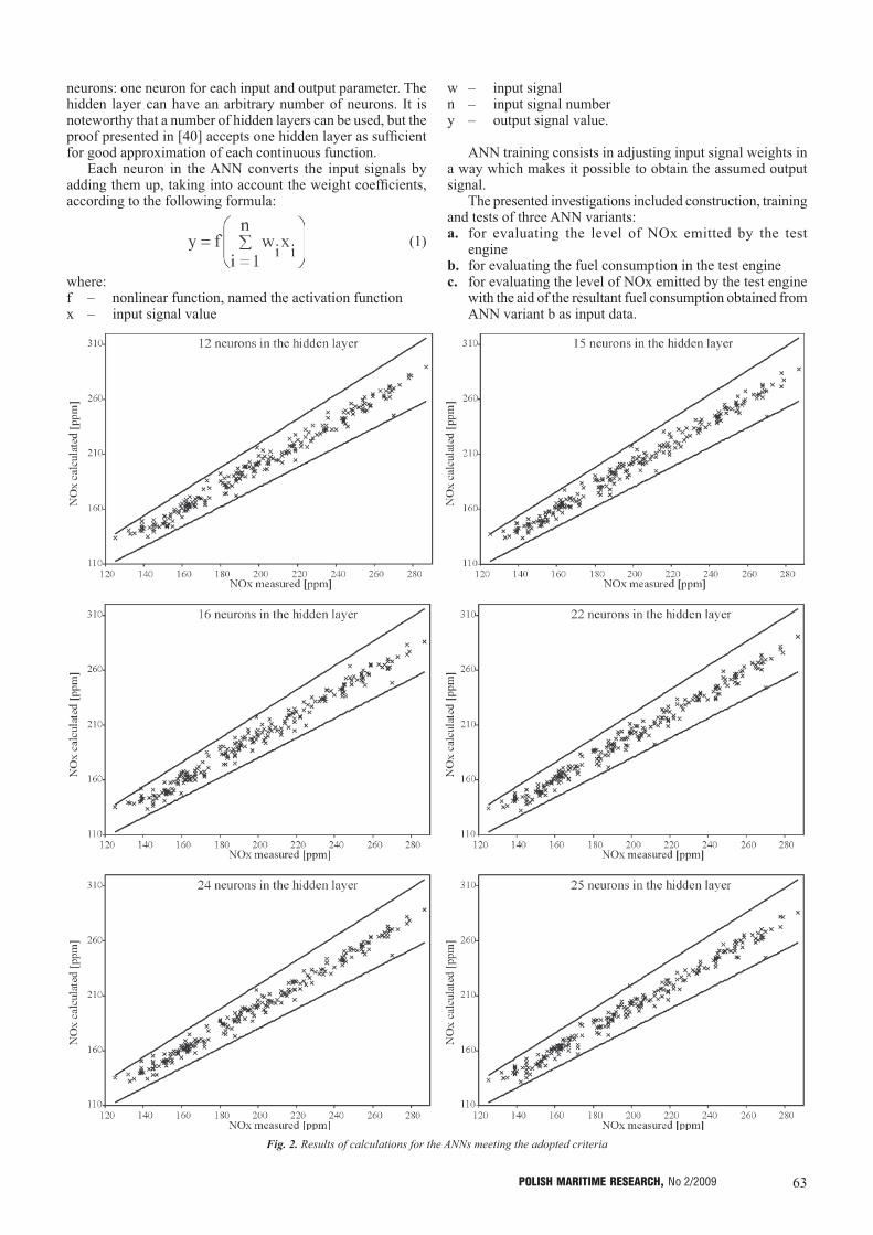
63POLISH MARITIME RESEARCH, No 2/2009
neurons: one neuron for each input and output parameter. The hidden layer can have an arbitrary number of neurons. It is noteworthy that a number of hidden layers can be used, but the proof presented in [40] accepts one hidden layer as sufficient for good approximation of each continuous function.
Each neuron in the ANN converts the input signals by adding them up, taking into account the weight coefficients, according to the following formula:
(1)
where:f – nonlinear function, named the activation functionx – input signal value
w – input signaln – input signal numbery – output signal value.
ANN training consists in adjusting input signal weights in a way which makes it possible to obtain the assumed output signal.
The presented investigations included construction, training and tests of three ANN variants:a. for evaluating the level of NOx emitted by the test
engineb. for evaluating the fuel consumption in the test enginec. for evaluating the level of NOx emitted by the test engine
with the aid of the resultant fuel consumption obtained from ANN variant b as input data.
Fig. 2. Results of calculations for the ANNs meeting the adopted criteria
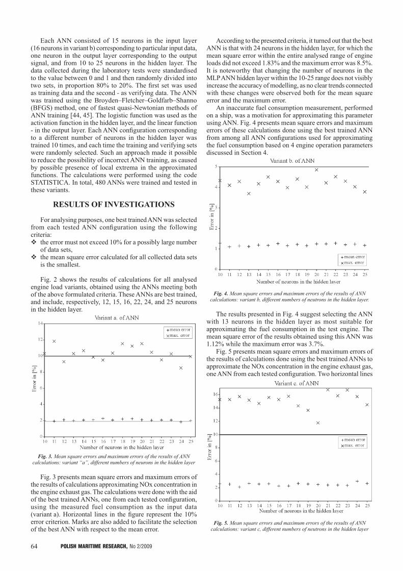
64 POLISH MARITIME RESEARCH, No 2/2009
Each ANN consisted of 15 neurons in the input layer (16 neurons in variant b) corresponding to particular input data, one neuron in the output layer corresponding to the output signal, and from 10 to 25 neurons in the hidden layer. The data collected during the laboratory tests were standardised to the value between 0 and 1 and then randomly divided into two sets, in proportion 80% to 20%. The first set was used as training data and the second - as verifying data. The ANN was trained using the Broyden–Fletcher–Goldfarb–Shanno (BFGS) method, one of fastest quasi-Newtonian methods of ANN training [44, 45]. The logistic function was used as the activation function in the hidden layer, and the linear function - in the output layer. Each ANN configuration corresponding to a different number of neurons in the hidden layer was trained 10 times, and each time the training and verifying sets were randomly selected. Such an approach made it possible to reduce the possibility of incorrect ANN training, as caused by possible presence of local extrema in the approximated functions. The calculations were performed using the code STATISTICA. In total, 480 ANNs were trained and tested in these variants.
RESULTS OF INVESTIGATIONS
For analysing purposes, one best trained ANN was selected from each tested ANN configuration using the following criteria:� the error must not exceed 10% for a possibly large number
of data sets,� the mean square error calculated for all collected data sets
is the smallest.
Fig. 2 shows the results of calculations for all analysed engine load variants, obtained using the ANNs meeting both of the above formulated criteria. These ANNs are best trained, and include, respectively, 12, 15, 16, 22, 24, and 25 neurons in the hidden layer.
Fig. 3. Mean square errors and maximum errors of the results of ANN calculations: variant “a”, different numbers of neurons in the hidden layer
Fig. 3 presents mean square errors and maximum errors of the results of calculations approximating NOx concentration in the engine exhaust gas. The calculations were done with the aid of the best trained ANNs, one from each tested configuration, using the measured fuel consumption as the input data (variant a). Horizontal lines in the figure represent the 10% error criterion. Marks are also added to facilitate the selection of the best ANN with respect to the mean error.
According to the presented criteria, it turned out that the best ANN is that with 24 neurons in the hidden layer, for which the mean square error within the entire analysed range of engine loads did not exceed 1.83% and the maximum error was 8.5%. It is noteworthy that changing the number of neurons in the MLP ANN hidden layer within the 10-25 range does not visibly increase the accuracy of modelling, as no clear trends connected with these changes were observed both for the mean square error and the maximum error.
An inaccurate fuel consumption measurement, performed on a ship, was a motivation for approximating this parameter using ANN. Fig. 4 presents mean square errors and maximum errors of these calculations done using the best trained ANN from among all ANN configurations used for approximating the fuel consumption based on 4 engine operation parameters discussed in Section 4.
Fig. 4. Mean square errors and maximum errors of the results of ANN calculations: variant b, different numbers of neutrons in the hidden layer.
The results presented in Fig. 4 suggest selecting the ANN with 13 neurons in the hidden layer as most suitable for approximating the fuel consumption in the test engine. The mean square error of the results obtained using this ANN was 1.12% while the maximum error was 3.7%.
Fig. 5 presents mean square errors and maximum errors of the results of calculations done using the best trained ANNs to approximate the NOx concentration in the engine exhaust gas, one ANN from each tested configuration. Two horizontal lines
Fig. 5. Mean square errors and maximum errors of the results of ANN calculations: variant c, different numbers of neutrons in the hidden layer
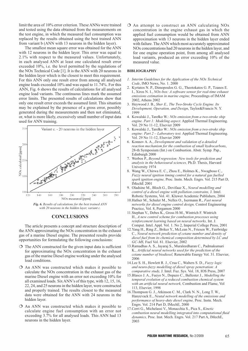
65POLISH MARITIME RESEARCH, No 2/2009
limit the area of 10% error criterion. These ANNs were trained and tested using the data obtained from the measurements on the test engine, in which the measured fuel consumption was replaced by the results obtained using the best trained ANN from variant b (ANN with 13 neurons in the hidden layer).
The smallest mean square error was obtained for the ANN with 12 neurons in the hidden layer. This error was equal to 2.1% with respect to the measured values. Unfortunately, in each analysed ANN at least one calculated result error exceeded 10%, i.e. the level permitted by the regulations of the NOx Technical Code [1]. It is the ANN with 20 neurons in the hidden layer which is the closest to meet this requirement. For this ANN only one result error from among all analysed engine loads exceeded 10% and was equal to 11.74%. For this ANN, Fig. 6 shows the results of calculations for all analysed engine load variants. The continuous lines mark the assumed error limits. The presented results of calculations show that only one result error exceeds the assumed limit. This situation may be explained by the presence of a gross error, possibly generated during the measurements and then not eliminated, or, what is more likely, excessively small number of input data used for ANN training.
Fig. 6. Results of calculations for the best trained ANN with 20 neurons in the hidden layer, variant c.
CONCLUSIONS
The article presents a concept and structure description of the ANN approximating the NOx concentration in the exhaust gas of a marine Diesel engine. The presented results provide opportunities for formulating the following conclusions:
� The ANN constructed for the given input data is sufficient for approximating the NOx concentration in the exhaust gas of the marine Diesel engine working under the analysed load conditions.
� An ANN was constructed which makes it possible to calculate the NOx concentration in the exhaust gas of the marine Diesel engine with an error not exceeding 10% for all examined loads. Six ANN’s of this type, with 12, 15, 16, 22, 24, and 25 neurons in the hidden layer, were constructed and properly trained. The results closest to the measured data were obtained for the ANN with 24 neurons in the hidden layer.
� An ANN was constructed which makes it possible to calculate engine fuel consumption with an error not exceeding 3.7% for all analysed loads. This ANN had 13 neurons in the hidden layer.
� An attempt to construct an ANN calculating NOx concentration in the engine exhaust gas in which the applied fuel consumption would be obtained from ANN approximation with 13 neurons in the hidden layer ended with failure. The ANN which most accurately approximated NOx concentrations had 20 neurons in the hidden layer, and for one engine operation point, from among all analysed load variants, produced an error exceeding 10% of the measured value.
BIBLIOGRAPHY
1. Interim Guidelines for the Application of the NOx Technical Code, IMO News, No. 1. 2000
2. Kyrtatos N. P., Dimopoulos G. G., Theotokatos G. P., Tzanos E. I., Xiros N. I., NOx-box: A software sensor for real-time exhaust emissions estimation in marine engine, Proceedings of IMAM 2002, Athens 2002
3. Heywood J. B., Sher E., The Two-Stroke Cycle Engine. Its Development, Operation, and Design, Taylor&Francis N. Y. 1999
4. Kowalski J., Tarełko W.: NOx emission from a two-stroke ship engine. Part 1: Modeling aspect. Applied Thermal Engineering. Vol. 29 No 11-12, Elsevier 2009
5. Kowalski J., Tarełko W.: NOx emission from a two-stroke ship engine: Part 2 – Laboratory test. Applied Thermal Engineering. Vol. 29 No 11-12, Elsevier 2009
6. Konnov A. A., Development and validation of a detailed reaction mechanism for the combustion of small hydrocarbons, 28-th Symposium (Int.) on Combustion. Abstr. Symp. Pap., Edinburgh 2000
7. Werbos P., Beyond regression: New tools for prediction and analysis in the behavioural sciences, Ph.D. Thesis, Harvard University 1974
8. Wang W., Chirwa E. C., Zhou E., Holmes K., Nwagboso C., Fuzzy neural ignition timing control for a natural gas fuelled spark ignition engine, Proc. Instn. Mech. Engrs. Vol. 215 Part D, IMechE 2001
9. Oladsine M., Bloch G., Dovifaaz X., Neural modelling and control of a diesel engine with pollution constrains, J. Intel. Robotic Systems, Vol. 41. Kluwer Academic Publishers, 2004
10. Hafner M., Schuler M., Nelles O., Isermann R., Fast neural networks for diesel engine control design, Control Engineering Practice, Vol. 8, Pergamon 2000
11. Stephan V., Debes K., Gross H-M., Wintrich F. Wintrich H., A new control scheme for combustion processes using reinforcement learning based on neural networks, Int. J. Comput. Intel. Appl. Vol. 1. No 2, Imperial College Press, 2001
12. Yang H., Ring Z., Briker Y., McLean N., Friesen W., Fairbridge C., Neural network prediction of cetane number and density of diesel fuel from its chemical composition determined by LC and GC-MS, Fuel Vol. 81. Elsevier, 2002
13. Ramadhas A. S., Jayaraj S., Muraleedharan C., Padmakumari K., Artificial neural networks used for the prediction of the cetane number of biodiesel, Renewable Energy Vol. 31. Elsevier, 2006
14. Lee S. H., Howlett R. J., Crua C., Walters S. D., Fuzzy logic and neuro-fuzzy modelling of diesel spray penetration: A comparative study, J. Intel. Fuz. Sys. Vol. 18, IOS Press, 2007
15. Blasco J. A., Fueyo N., Dopazo C., Ballester J., Modelling the temporal evolution of a reduced combustion chemical system with an artificial neural network, Combustion and Flame, Vol 113, Elsevier, 1998
16. Thompson G. J., Atkinson C. M., Clark N. N., Long T. W., Hanzevack E., Neutal network modelling of the emissions and performance of heavy-duty diesel engine, Proc. Instn. Mech. Engrs. Vol. 214 Part D, IMechE, 2000
17. Cerri G., Michelassi V., Monacchia S., Pica S., Kinetic combustion neural modelling integrated into computational fluid dynamics, Proc. Inst. Mech. Engrs. Vol. 217 Part A, IMechE, 2003

66 POLISH MARITIME RESEARCH, No 2/2009
18. Shenvi N., Geremia J. M., Rabitz H., Efficient chemical kinetic modelling through neural network maps, Journal of Chemical Physics Vol. 120, No 21. American Institute of Physics, 2004
19. Galindo J., Luja´n J. M., Serrano J. R., Hernandez L., Combustion simulation of turbocharger HSDI Diesel engines during transient operation using neural networks, Applied Thermal Engineering Vol. 25,Elsevier, 2005
20. Sen B. A., Menon S., Turbulent premixed flame modeling using artificial neural networks based chemical kinetics, Proceedings of the Combustion Institute Vol. 32, Elsevier, 2009
21. Kesgin U., Genetic algorithm and artificial neural network for engine optimisation of efficiency and NOx emission, Fuel Vol. 83, Elsevier, 2004
22. Sayin C., Ertunc H. M., Hosoz M., Kilicaslan I., Canakci M., Performance and exhaust emissions of a gasoline engine using artificial neural network, Applied Thermal Engineering Vol. 27, Elsevier, 2007
23. Al-Hinti I., Samhouri M., Al-Ghandoor A., Sakhrieh A., The effect of boost pressure on the performance characteristics of a diesel engine: A neuro-fuzzy approach, Applied Energy Vol. 86, Elsevier, 2009
24. Parlak A., Islamoglu Y., Yasar H., Egrisogut A., Application of artificial neural network to predict fuel consumption and temperature for a diesel engine, Applied Thermal Engineering Vol. 26, Elsevier, 2006.
25. Wang S., D.L. Yu., Adaptive RBF network for parameter estimation and stable air–fuel ratio control, Neural Networks Vol. 21. Elsevier, 2008
26. Ghobadian B., Rahimi H., Nikbakht A. M., Najafi G., Yusaf T. F., Diesel engine performance and exhaust emission analysis using waste cooking biodiesel fuel with an artificial neural network, Renewable Energy Vol. 34, Elsevier, 2009
27. Atashkari K., Nariman-Zadeh N., Gölcü M., Khalkhali A., Jamali A., Modelling and multi-objective optimization of a variable valve-timing spark-ignition engine using polynomial neural networks and evolutionary algorithms, Energy Conversion and Management, Vol. 48, Elsevier, 2007
28. Najafi G., Ghobadian B., Tavakoli T., Buttsworth D. R., Yusaf T. F., Faizollahnejad M., Performance and exhaust emissions of a gasoline engine with ethanol blended gasoline fuels using artificial neural network, Applied Energy Vol. 86, Elsevier, 2009
29. Wu J-D., Liu C-H., An expert system for fault diagnosis in internal combustion engines using wavelet packet transform and neural network, Expert Systems with Applications Vol. 36, Elsevier, 2009
30. Heywood J. B., Internal Combustion Engine Fundamentals, McGraw-Hill 1988
31. Bebara L., Kermesa V., Stehlika P., Canekb J., Oralc J., Low NOx burners—prediction of emissions concentration based on design, measurements and modeling, Waste Management No. 22/2002, Elsevier Science Inc. 2002
32. Reynolds J. P., Jeris J., Theodore L., Handbook of chemical and environmental engineering calculations, Willey-Interscience, New Jersey 2007
33. Egolfopoulos F. N., Validation of nitrogen kinetics in high pressure fames, Energy Conversion & Management No. 42/2001, Elsevier Science Inc. 2001
34. Lyle K. H., Tseng K. L., Gore J. P., Laurendeau N. M., A study of pollutant emission characteristics of partially premixed turbulent jet flames, Combustion and Flame No. 116/1999, Elsevier Science Inc. 1999
35. Kuo K. K., Principles of combustion, Wiley. New Jersey 200536. Kowalski J., Tarelko W., Nitric Oxides emission estimation
based on measuring of work parameters of ship two-stroke engine, Proceedings of 2nd International Conference on Marine Research and Transportation. Ischia Naples Italy. 2007. Session C
37. Barlow R. S., Karpetis A. N., Frank J. H., Scalar profiles and no formation in laminar opposed-flow partially premixed methane/air flames, Combustion and Flame No. 127/2001, Elsevier Science Inc. 2001
38. Bowman C. T, Hanson R. K., Gardiner W. C., Lissianski V., Frenklach M., Goldenberg M., Smith G. P., Crosley D. R., Golden D. M., GRI-Mech 2.11 An optimized detailed chemical reaction mechanism for methane combustion and NO formation and re-burning, Topical Report Gas Research Institute 6/94 - 2/96
39. Curran H. J., Gaffuri P., Pitz W. J., Westbrook C. K., A comprehensive modeling study of n-heptane oxidation, Combustion and Flame No. 114/1998, Elsevier Science Inc. 1998
40. Masters T., Practical neural network recipes in C++, Academic Press Inc., 1993
41. Marine Engine IMO Tier II Programme 2009, MAN Netherland 2009
42. Kowalski J., The NOx emission estimation by artificial neural network: the results, Journal of KONES, Vol. 15, Warsaw 2008
43. Kowalski J., The NOx emission estimation by artificial neural network: the analyze, Journal of KONES, Vol. 15, Warsaw 2008
44. Ghobadian B., Rahimi H., Nikbakht A. M., Najafi G,, Yusaf T. F., Diesel engine performance and exhaust emission analysis using waste cooking biodiesel fuel with an artificial neural network, Renewable Energy Vol. 34, Elsevier Science Inc. 2009
45. Svozil D., Kvasnicka V., Pospichal J., Introduction to multi-layer feed-forward neural networks, Chemometrics and intelligent laboratory systems Vol. 39, Elsevier 1997
CONTACT WITH THE AUTHORS
Jerzy Kowalski, Ph.D.Department of Engineering Sciences
Gdynia Maritime UniversityMorska 81/87
81-225 Gdynia, POLANDe-mail : [email protected]

67POLISH MARITIME RESEARCH, No 2/2009
INTRODUCTION
Stowing general cargoes on ships contains several operations associated with appropriate location of the cargoes and their securing. Contemporary technology used in cargo shipping aims at elimination of stowing errors by standardizing cargo units as well as appropriate adjusting ship structures. It makes it possible to expand automation of cargo handling in ports. The most popular have become containers which have dominated cargo transport by sea. Technology of handling and securing containers on ships makes it possible to entirely eliminate workforce and achieve this way very high effectiveness. Several millions of containers are yearly handled in sea container terminals which employ a few dozen percent smaller number of workers as compared with traditional general cargo terminals. This constitutes a huge technological progress but it also posseses its own limitations. A part of cargoes, called non-standard ones, requires - and will require in the future - an individual approach and significant human work outlay. Among them heavy cargo pieces, large gabarite loads as well as other loads in non-standard packing, are numbered.
Stowing techniques of non-standard cargoes are rarely described in ship cargo handling documentation, especially in Cargo Securing Manual. Therefore persons responsible for loading are forced to rely on other available documents and their knowledge of ship, cargo and own experience. Their responsibility is high as stowing errors are often associated with high cargo losses and in extreme cases they can cause
Accuracy analysis of stowing computations for securing non-standard cargoes on ships
according to IMO CSS Code
Jerzy KabacińskiBogusz Wiśnicki, Ph. D.Maritime University of Szczecin
ABSTRACT
The article takes up a subject of effectiveness of securing arrangements while stowing non-standard cargoes on ships. Accuracy analysis of stowing calculations was based on procedures proposed by Code of Safe Practice for Cargo Stowage and Securing – CSS Code. Detailed calculations of forces and moments related to lashings, which prevents non-standard cargo against transverse tipping, were performed. Some simplifications were proven that may result in underestimating or overstating the calculated righting moment, which decides of safety margin of securing non-standard cargoes. The alternative more reliable
procedure, without simplifications, was proposed.
Keywords: safety of transportation; stowing; cargo securing; non-standard cargoes; lashing
loss of ship’s floatability. The principle is that each piece of non-standard cargo requires seperate stowing calculations and selection of a suitable securing technique with the use of appropriate lashing equipment. Appropriate know-how in the area is crucial.
In present there are a few IMO (Internatonal Maritime Organisation) documents useful in preparing stowing plans for non-standard cargoes. Code of Safe Practice for Cargo Stowage and Securing – CSS Code is the most important. The Code contains example procedures for stowing calculations, which make it possible to select proper securing equipment. In 2002 during 75th session of MSC/IMO subcommitee some important changes were introduced to Appendix13, titled „Methods to assess the efficiency of securing arrangements for non-standardized cargoes”. In the Appendix formulae and tables are included for calculation of forces intended to protect against shifting and overturning a non-standard cargo. Knowledge of such forces makes it possible to select an appropriate number and quality of securing stays.
However the formulae and tables given in the Appendix in question contain some relatively important simplifications which affect results of calculations, that may result in lowering effectiveness of securing the cargo. The simplifications concern calculations for determination of forces occurring in stays intended to protect cargo against transverse overturning. The below presented analysis is aimed at making comparison of accuracy of calculations performed with the use of the CSS Code procedures and alternative ones.
POLISH MARITIME RESEARCH 2(60) 2009 Vol 16; pp. 67-7110.2478/v10012-008-0024-6

68 POLISH MARITIME RESEARCH, No 2/2009
CALCULATIONS OF MOMENTS IN STAYS WHICH SECURE NON-STANDARD CARGO AGAINST TRANSVERSE OVERTURNING
The CSS Code recommends to use the below given inequality to control whether the cargo securing stays protect it against overturning in port or starboard direction :
(1)
where:Fy – transverse cargo overturning force [kN]d – arm of action of overturnig force [m]
(usually assumed equal to a half of the cargo height d = h/2)
b = e/2 [m], [where: e – transverse distance between supports of a cargo (cargo breadth)]
m – mass of a cargo unit [t]g = 9.81 m/s2 (gravity acceleration)CS1, CS2, ….CSn – forces in staysc1, c2, …..cn – arms of action of forces in stays.
The important assumption given in the CSS Code indicates that the angles α and β, between the stay and ship’s deck, (the vertical angle α between and perpendicular to ship central line, and the horizontal angle β) are to satisfy the following requirement (Fig. 1): α ≥ 45° or β ≤ 45°.
Additionally, forces in stays are calculated as a fraction of the maximum securing load MSL according to the formula:
(2)
The CSS Code also indicates a way to simplification of calculations by making assumption that values of arms of forces in stays are approximately equal to the cargo breadth e:
c1 ≈ c2 ≈ ….. ≈ cn ≈ eHence the inequality (1) can be substituted by the
following:
(3)
Fig. 1. Moment of single stay which prevents against cargo overturning (According to the authors’ elaboration).
Course of calculations which led to formulation of the inequality (3) which describes forces acting in the case of transverse overturning the cargo, can be analyzed by using simple calculations. The inequality illustrates the relation between the cargo overturning moment which acts crosswise the ship and the moment which resist the former. This is the moment associated with action of the gravity force m·g and sum of the moments associated with forces in oblique cargo securing stays, My. The stays must be directed towards the opposite side relative to direction of action of the overturning force.
(4)
The moment of force in single stay, which resist the overturning, is equal to:
(5)
where:CS – force in single stay [kN]c – arm of force [m]a – vertical projection of the stay line onto the deck plane [m].
The formula is correct only for the angle β equal to 0° (i.e. when the stay is perpendicular to ship’s central plane). Otherwise, at determining the moment My, the parameter a should be substituted by the product a·cosβ, and the formula in question finally takes the form as follows (Fig. 2) :
(6)
Fig. 2. Decomposition of the force acting in stay which resist the overturning of cargo (According to the authors’ elaboration).
On substitution of a by :
the following was obtained:
(7)
where:α – vertical angle of stay β – horizontal angle of stay
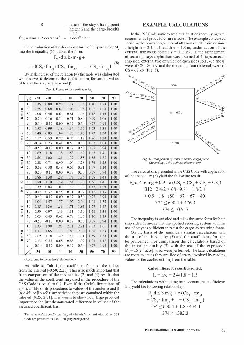
69POLISH MARITIME RESEARCH, No 2/2009
R – ratio of the stay’s fixing point height h and the cargo breadth e, h/e
fmy = sinα + R·cosα·cosβ – a coefficient.
On introduction of the developed form of the parameter �My into the inequality (3) it takes the form:
(8)
By making use of the relation (4) the table was elaborated which serves to determine the coefficient fmy for various values of R and the stay angles α and β.
Tab. 1. Values of the coefficient fmy
β α -30 -10 0 10 30 50 70 90
R =
1.0
10 0.35 0.80 0.98 1.14 1.35 1.40 1.28 1.0030 0.25 0.68 0.87 1.03 1.25 1.32 1.24 1.0050 0.06 0.46 0.64 0.81 1.06 1.18 1.16 1.0070 -0.20 0.16 0.34 0.51 0.80 0.99 1.06 1.0090 -0.50 -0.17 0.00 0.17 0.50 0.77 0.94 1.00
R =
1.2
10 0.52 0.99 1.18 1.34 1.52 1.53 1.34 1.0030 0.40 0.85 1.04 1.20 1.40 1.43 1.30 1.0050 0.17 0.59 0.77 0.93 1.17 1.26 1.20 1.0070 -0.14 0.23 0.41 0.58 0.86 1.03 1.08 1.0090 -0.50 -0.17 0.00 0.17 0.50 0.77 0.94 1.00
R =
1.4
10 0.69 1.18 1.38 1.53 1.69 1.65 1.41 1.0030 0.55 1.02 1.21 1.37 1.55 1.55 1.35 1.0050 0.28 0.71 0.90 1.06 1.28 1.34 1.25 1.0070 -0.09 0.30 0.48 0.65 0.91 1.07 1.10 1.0090 -0.50 -0.17 0.00 0.17 0.50 0.77 0.94 1.00
R =
1.6
10 0.86 1.38 1.58 1.73 1.86 1.78 1.48 1.0030 0.70 1.19 1.39 1.54 1.70 1.66 1.41 1.0050 0.39 0.84 1.03 1.19 1.39 1.43 1.29 1.0070 -0.03 0.37 0.55 0.71 0.97 1.12 1.13 1.0090 -0.50 -0.17 0.00 0.17 0.50 0.77 0.94 1.00
R =
1.8
10 1.04 1.57 1.77 1.92 2.04 1.91 1.55 1.0030 0.85 1.36 1.56 1.71 1.85 1.77 1.47 1.0050 0.50 0.97 1.16 1.31 1.50 1.51 1.34 1.0070 0.03 0.43 0.62 0.78 1.03 1.16 1.15 1.0090 -0.50 -0.17 0.00 0.17 0.50 0.77 0.94 1.00
R =
2.0
10 1.33 1.90 1.97 2.11 2.21 2.03 1.61 1.0030 1.11 1.65 1.73 1.88 2.00 1.88 1.53 1.0050 0.69 1.18 1.29 1.44 1.61 1.59 1.38 1.0070 0.13 0.55 0.68 0.85 1.09 1.21 1.17 1.0090 -0.50 -0.17 0.00 0.17 0.50 0.77 0.94 1.00β α -30 -10 0 10 30 50 70 90
(According to the authors’ elaboration)
As indicates Tab. 1, the coefficient fmy take the values from the interval [-0.50; 2.21]. This is so much important that from comparison of the inequalities (2) and (5) results that the value of the coefficient fmy, used in the procedure of the CSS Code is equal to 0.9. Even if the Code’s limitations of applicability of its procedures to values of the angles α and β (α ≥ 45° or β ≤ 45°)1 are satisfied they are contained within the interval [0.25; 2.21]. It is worth to show how large practical importance the just demonstrated difference in values of the assumed coefficient, has.
EXAMPLE CALCULATIONS
In the CSS Code some example calculations complying with recommended procedures are shown. The example concerned securing the heavy cargo piece of 68 t mass and the dimensions : height h = 2.4 m, breadth e = 1.8 m, under action of the external transverse force Fy = 312 kN. In the arrangement of securing stays application was assumed of 4 stays on each ship side, external two of which on each side (no.1, 4, 5 and 8) were of CS = 80 kN, and the remaining four (internal) were of CS = 67 kN (Fig. 3).
Fig. 3. Arrangement of stays to secure cargo piece (According to the authors’ elaboration).
The calculations presented in the CSS Code with application of the inequality (2) yield the following result:
Fy·d ≤ b·m·g + 0.9 · e (CS1 + CS2 + CS3 + CS4)312 · 2.4/2 ≤ 68 · 9.81 · 1.8/2 ++ 0.9 · 1.8 · (80 + 67 + 67 + 80)
374 ≤ 600.4 + 476.3374 ≤ 1076.7
The inequality is satisfied and takes the same form for both ship sides. It means that the applied securing system with the use of stays is sufficient to resist the cargo overturning force.
On the basis of the same data similar calculations with the use of the inequality (5) and the coefficients fmy can be performed. For comparison the calculations based on the initial inequality (3) with the use of the expression My = CS(e + acosβ)sinα, were performed. The latter calculations are more exact as they are free of errors involved by reading values of the coefficient fmy from the table.
Calculations for starboard sideR = h/e = 2.4/1.8 = 1.3
The calculations with taking into account the coefficients fmy yield the following relationship:
Fy·d ≤ b·m·g + e (CS1 · fmy1 + CS2 · fmy2 +... + CSn · fmyn)
374 ≤ 600.4 + 1.8 · 434.4374 ≤ 1382.3 1 The values of the coefficient fmy, which satisfy the limitation of the CSS
Code are presented in Tab. 1 on gray background.

70 POLISH MARITIME RESEARCH, No 2/2009
The exact calculations, i.e. without simplifications, yield the following relationship:
Fy·d ≤ b·m·g + My1 + My2 +... + Myn
374 ≤ 600.4 + 804.0374 ≤ 1404.4
Tab. 2. Strength calculations for starboard side
No.
of s
tay
CS α β
a =
h/tg
α
c =
(e+a
·cos
β)si
nα
My =
CS·
c
fmy
CS·
fmy
1 80 40 30 2.86 2.75 220.0 1.48 118.42 67 50 20 2.01 2.83 189.6 1.54 103.23 67 50 20 2.01 2.83 189.6 1.54 103.24 80 40 40 2.86 2.56 204.8 1.37 109.6
804.0 434.4
(According to the authors’ elaboration)
Calculations for port side
Tab. 3. Strength calculations for port side
No.
of s
tay
CS α β
a =
h/tg
α
c =
(e+a
·cos
β)si
nα
My =
CS·
c
fmy
CS·
fmy
5 80 40 30 2.86 2.75 220.0 1.48 118.46 67 20 30 6.59 2.57 172.2 1.38 92.57 67 20 10 6.59 2.83 189.6 1.47 98.58 80 40 30 2.86 2.75 220.0 1.48 118.4
801.8 427.8
(According to the authors’ elaboration)
The calculations with taking into account the coefficients fmy yield the following relationship:
374 ≤ 600.4 + 1.8 · 427.8374 ≤ 1370.4
The exact calculations, i.e. without simplifications, yield the following relationship:
374 ≤ 600.4 + 801.8374 ≤ 1402.2
The obtained inequalities for port and starboard side differ to each other only a little. All the results indicate that the applied securing system with the use of stays is sufficient to resist cargo overturning force. In all variants the securing safety margin, i.e. the difference between overturning moment and righting moment, is much greater than that calculated according to the CSS Code.
CONCLUSIONS
On the basis of the performed accuracy analysis of strength calculations of securing the non-standard cargoes with the use of stays the following detail conclusions can be offerred:
� The procedure for calculations of the moment resisting the transverse force which tends to overturn the non-standard cargo, recommended by the CSS Code, is simple in use but loaded by a large error resulting from the applied simplifications.
� The first important simplification in the CSS Code is the application of the constant coefficient equal to 0,9 in the inequality (1) whereas in reality it takes values from the interval [-0.50; 2.21].
� Succesive simplification introduced in the CSS Code is the asssumption that values of arms of forces acting in stays are approximately equal to the cargo breadth e, that results in the recommendation on using the inequality (2) to calculations.
� Applicability of the CSS Code procedures is limited only to the stays the angles α and β of which, formed by stay and deck and the line perpendicular to ship’s central line, are to satisfy the requirement : (α ≥ 45° or β ≤ 45°); in practice the limitation eliminates certain stowing techniques.
� In the presented example calculations the application of the asummed CSS Code simplifications results in lowering, by about 300 kNm, real value of the moment resisting the transverse force which tends to overturn a non-standard cargo piece; this may be compared with neglection of the force acting in one stay at least.
� In practice, the application of the CSS Code procedures may be connected with lowering or overstating the calculated moment as the procedure takes into account only number and nominal strength of stays and does not differentiate them regarding the angle which they form with ship’s deck and straight line perpendicular to ship’s central line.; this is why the same result was obtained for the same number of stays on port and starboard side.
Application of the inequality (5) together with Tab. 1 which serves to determine the coefficient fmy for various values of R and the angles α and β of securing stays, is proposed as an alternative procedure for calculation of moments in stays which prevent the non-standard cargo from overturning, which is free of errors of excessive simplifications.Results obtained by means of the procedure only a little differ from those accurate calculated with the use of trigonometric functions. The observed differences result from application of linear interpolation to reading values of the coefficient fmy from Tab. 1, whereas in reality values of the coeffcient vary non-linearly.
Application of the alternative procedure should not be limited to any range of the angles α and β formed by stays. However it is important to observe that for certain stays which are characterized by negative values of the angle α, force in such stays, instead to prevent the cargo against transverse overturning, can co-operate with the overturning force. It can so happen if the coefficient fmy takes negative values. Therefore as a rule the system of securing the cargo by means of stays directed upwards from the level of their fixing points at the cargo, should be avoided.

71POLISH MARITIME RESEARCH, No 2/2009
The proposed alternative procedure would improve safety of securing non-standard cargoes. Accurate calculations of moments resisting transverse overturning the cargo would be transformed to stowing decisions, i.e choice of number and strength of stays as well as a way of their fixing. As a result of this, errors in the form of unnecessary increasing the safety margin of cargo securing would be avoided, that is connected with additional labour consumption and cost of stowing. Moreover, the procedure makes it possible to avoid errors of lowering the safety margin which may result in overturning the cargo and further consequences.
BIBLIOGRAPHY
1. Code of Safe Practice for Cargo Stowage and Securing (CSS Code), International Maritime Organization (IMO IA292E), 2003
2. Guidelines For The Preparation Of The Cargo Securing Manual, International Maritime Organization (IMO I298E), 1997.
CONTACT WITH THE AUTHORSBogusz Wiśnicki, Ph. D.
Maritime University of SzczecinWały Chrobrego 1-2
70-500 Szczecin, POLANDe-mail: [email protected]
72 POLISH MARITIME RESEARCH, No 2/2009
INTRODUCTION
As results from subject-matter literature fire toxic hazard in shipboard living and service accommodations is high. Statistical data indicate that 36% fires on ships take place just in living and service accommodations.
Fig. 1. Location of fire sources on ships [1]
The mentioned hazard due to toxic thermal decomposition of materials installed in shipboard living accommodations is also confirmed by consequences of real fires. The fire on the ferry ship „Scandinavian Star” has been numbered among the most tragic accidents of the kind. Out of 485 persons present on board 158 died as a result of fire. On the basis of casualty investigations it was stated that in about 94% cases decease was caused by action of carbon oxide and hydrogen cyanide emitted
Selection of outfitting and decorative materials for ship living accommodations from
the point of view of toxic hazard in the initial phase of fire progress
Renata Dobrzyńska, Ph. D.West Pomeranian University of Technology, Szczecin
ABSTRACT
Upholstery furniture and bedding components which presently are required to satisfy conditions of resistance to only small fire setting sources, really constitute a serious source of toxic hazard. The proposed method of toxic hazard assessment in the initial phase of fire progress, due to thermal decomposition and combustion of materials, makes appropriate selection of outfitting materials for shipboard living and service accommodations already in ship design phase, possible. Practical application of the proposed algorithm of selection procedure of suitable outfitting and decorative materials intended for shipboard living
accommodations would decrease fire toxic hazard level in such accommodations.
Keywords: fire safety of ship; quantitative method of toxic hazard assessment
during thermal decomposition and combustion of materials used for the outfitting of cabins and corridor [2].
Outfitting materials (products) introduce serious thermal, smokiness and toxic risk. Yet upholstery furniture, decorative materials, bedding components are not covered by any test from the point of view of fire toxic hazard introduced by them – see IMO MSC. 61(67) resolution [3]. They are only to satisfy requirements for fire resistance against action of small fire setting sources. An upholstery system satisfies the Code requirements if it will pass the test of smouldering cigarette and flame equivalent of burning match. The exposure time to action of the flame is equal to 20s (Fig. 2). Enough to extend the time up to 30s to start the upholstery system intensive burning (Fig. 3).
It means that the considered upholstery system which satisfies the rule requirements, is resistant to action of small fire setting sources only for 20s. In spite of the so moderate criterion many upholstery systems do not satisfy it. Therefore some fire-proofing agents which cause larger emission of smoke and toxic substances during fire, are added [5].
During fire people are exposed to action of a mixture of toxic substances. On assumption of additive influence of such mixture of toxic substances on human organism their concentration values ci in atmosphere of fire zone are to fulfil the condition:
(1)
where: – limit concentration of i-th substance, g · m-3
POLISH MARITIME RESEARCH 2(60) 2009 Vol 16; pp. 72-7410.2478/v10012-008-0025-5
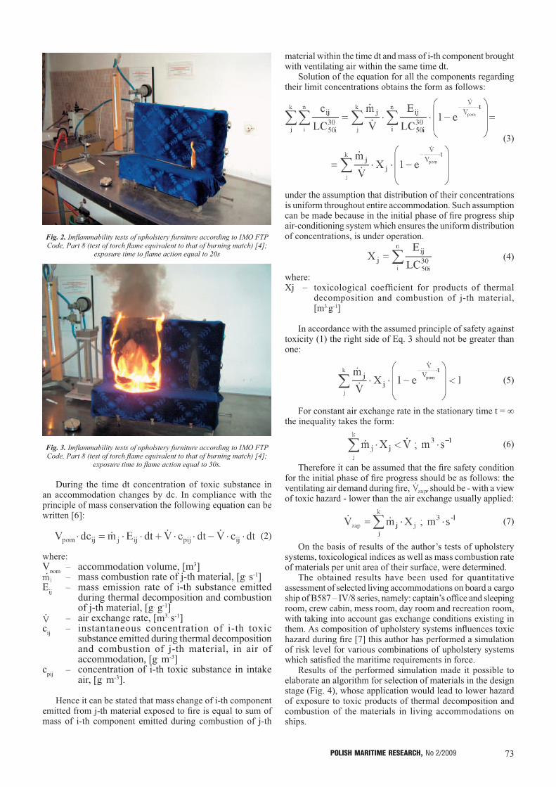
73POLISH MARITIME RESEARCH, No 2/2009
Fig. 2. Imflammability tests of upholstery furniture according to IMO FTP Code, Part 8 (test of torch flame equivalent to that of burning match) [4];
exposure time to flame action equal to 20s
Fig. 3. Imflammability tests of upholstery furniture according to IMO FTP Code, Part 8 (test of torch flame equivalent to that of burning match) [4];
exposure time to flame action equal to 30s.
During the time dt concentration of toxic substance in an accommodation changes by dc. In compliance with the principle of mass conservation the following equation can be written [6]:
(2)
where:Vpom – accommodation volume, [m3]
– mass combustion rate of j-th material, [g. s-1]Eij – mass emission rate of i-th substance emitted
during thermal decomposition and combustion of j-th material, [g. g-1]
– air exchange rate, [m3. s-1]cij – instantaneous concentration of i-th toxic
substance emitted during thermal decomposition and combustion of j-th material, in air of accommodation, [g. m-3]
cpij – concentration of i-th toxic substance in intake air, [g. m-3].
Hence it can be stated that mass change of i-th component emitted from j-th material exposed to fire is equal to sum of mass of i-th component emitted during combustion of j-th
material within the time dt and mass of i-th component brought with ventilating air within the same time dt.
Solution of the equation for all the components regarding their limit concentrations obtains the form as follows:
(3)
under the assumption that distribution of their concentrations is uniform throughout entire accommodation. Such assumption can be made because in the initial phase of fire progress ship air-conditioning system which ensures the uniform distribution of concentrations, is under operation.
(4)
where:Xj – toxicological coefficient for products of thermal
decomposition and combustion of j-th material, [m3.g-1]
In accordance with the assumed principle of safety against toxicity (1) the right side of Eq. 3 should not be greater than one:
(5)
For constant air exchange rate in the stationary time t = ∞ the inequality takes the form:
(6)
Therefore it can be assumed that the fire safety condition for the initial phase of fire progress should be as follows: the ventilating air demand during fire, , should be - with a view of toxic hazard - lower than the air exchange usually applied:
(7)
On the basis of results of the author’s tests of upholstery systems, toxicological indices as well as mass combustion rate of materials per unit area of their surface, were determined.
The obtained results have been used for quantitative assessment of selected living accommodations on board a cargo ship of B587 – IV/8 series, namely: captain’s office and sleeping room, crew cabin, mess room, day room and recreation room, with taking into account gas exchange conditions existing in them. As composition of upholstery systems influences toxic hazard during fire [7] this author has performed a simulation of risk level for various combinations of upholstery systems which satisfied the maritime requirements in force.
Results of the performed simulation made it possible to elaborate an algorithm for selection of materials in the design stage (Fig. 4), whose application would lead to lower hazard of exposure to toxic products of thermal decomposition and combustion of the materials in living accommodations on ships.

74 POLISH MARITIME RESEARCH, No 2/2009
CONCLUSIONS
� Upholstery furniture and bedding components which are presently required to satisfy conditions of resistance to only small fire setting sources, really constitute a serious source of toxic hazard.
� To quantitatively assess fire toxicity hazard in ship accommodations, knowledge of the following parameters is necessary: mass emission of toxic products of thermal decomposition
and combustion of materials, mass combustion rate of materials.
On the basis of mass emission the toxicological indices for products of thermal decomposition and combustion, Xj, can be determined.
� In the initial phase of fire progress fulfillment of the following condition:
is necessary in order to ensure fire toxic safety.� The proposed assessment method of toxic hazard resulting
from thermal decomposition and combustion of materials, makes appropriate selection of outfitting materials for ship living and service accommodations in ship design phase, possible.
� Practical application of the elaborated method and proposed algorithm of selection procedure of suitable outfitting and decorative materials intended for ship living accommodations, would decrease fire toxic hazard level in living and service accommodations on ships.
BIBLIOGRAPHY
1. Grzywaczewski Z., Załęcki S.: Fire fighting on ships (in Polish). Maritime Publishing House (Wydawnictwo Morskie), Gdynia 1982
2. Robinson A., Burgoyne J.H.: The Scandinavian Star Incident. A Case Study. IFE Journal, 1999
3. IMO: International Code of Fire Testing Procedures (in Polish), IMO Resolution MSC. 61(67), London 1998
4. IMO: Fire resistance tests of upholstery furniture according to FTP Code (in Polish), Part 8, IMO Res. A.652(16), London 1998
5. Dobrzyńska R.: Influence of applied amount of fire-proofing agents on emission of toxic products of thermal decomposition of polyurethane foams (in Polish). 42nd Scientific Congress of Polish Chemical Society and Polish Society of Chemical Engineers and Technicians, Rzeszów 1999
6. Dobrzyńska R.: Toxic hazard level evaluation of ship rooms during initial phase of fire progress. Marine Technology Transactions, vol. 16, 2005
7. Dobrzyńska R.: Toxic hazard level assessment of ship accommodations during initial phase of fire progress (in Polish). 8th Conference on Shipbuilding and Ocean Engineering – Development prospects of transport systems, Publ. of Szczecin Technical University, Szczecin 2006.
CONTACT WITH THE AUTHORRenata Dobrzyńska, Ph. D.
West Pomeranian University of Technology, SzczecinFaculty of Marine Technology
AL. Piastów 4171-065 Szczecin, POLAND
e-mail: [email protected]
Fig. 4. Algorithm of selection procedure of suitable outfitting and decorative materials intended for applying to living accommodations on ships

75POLISH MARITIME RESEARCH, No 2/2009
The Ship Handling Research and Training Centre at Ilawa is owned by the Foundation for Safety of Navigation and Environment Protection, which is a joint venture between the Gdynia Maritime University, the Gdansk University of Technology and the City of Ilawa.
Two main fields of activity of the Foundation are:
� Training on ship handling. Since 1980 more than 2500 ship masters and pilots from 35 countries were trained at Iława Centre. The Foundation for Safety of Navigation and Environment Protection, being non-profit organisation is reinvesting all spare funds in new facilities and each year to the existing facilities new models and new training areas were added. Existing training models each year are also modernised, that's why at present the Centre represents a modern facility perfectly capable to perform training on ship handling of shipmasters, pilots and tug masters.
� Research on ship's manoeuvrability. Many experimental and theoretical research programmes covering different problems of manoeuvrability (including human effect, harbour and waterway design) are successfully realised at the Centre.
The Foundation possesses ISO 9001 quality certificate.
Why training on ship handling?
The safe handling of ships depends on many factors - on ship's manoeuvring characteristics, human factor (operator experience and skill, his behaviour in stressed situation, etc.), actual environmental conditions, and degree of water area restriction.
Results of analysis of CRG (collisions, rammings and groundings) casualties show that in one third of all the human error is involved, and the same amount of CRG casualties is attributed to the poor controllability of ships. Training on ship handling is largely recommended by IMO as one of the most effective method for improving the safety at sea. The goal of the above training is to gain theoretical and practical knowledge on ship handling in a wide number of different situations met in practice at sea.
For further information please contact:The Foundation for Safety of Navigation and Environment Protection
Head office:36, Chrzanowskiego street80-278 GDAŃSK, POLANDtel./fax: +48 (0) 58 341 59 19
Ship Handling Centre:14-200 IŁAWA-KAMIONKA, POLAND
tel./fax: +48 (0) 89 648 74 90e-mail: [email protected]
e-mail: [email protected]

76 POLISH MARITIME RESEARCH, No 2/2009
GDANSK UNIVERSITY OF TECHNOLOGYis the oldest and largest scientific and technological academic institution in the Pomeranian region. The history of Gdansk University of Technology is marked by two basic dates, namely: October 6, 1904 and May 24, 1945.
The first date is connected with the beginning of the technical education at academic level in Gdansk. The second date is connected with establishing of Gdansk University of Technology, Polish state academic university. Gdansk University of Technology employ 2,500 staff, 1,200 whom are academics. The number of students approximates 20,000, most of them studying full-time. Their career choices vary from Architecture to Business and Management, from Mathematics and Computer Science to Biotechnology and Environmental Engineering, from Applied Chemistry to Geodesics and Transport, from Ocean Engineering to Mechanical Engineering and Ship Technology, from Civil Engineering to Telecommunication, Electrical and Control Engineering. Their life goals, however, are much the same - to meet the challenge of the changing world. The educational opportunities offered by our faculties are much wider than those of other Polish Technical universities, and the scientific research areas include all of 21st Century technology. We are one of the best schools in Poland and one of the best known schools in Europe – one that educates specialists excelling in the programming technology and computer methods used in solving complicated
scientific, engineering, organizational and economic problems. THE FACULTY OF OCEAN ENGINEERING
AND SHIP TECHNOLOGYThe Faculty of Ocean Engineering and Ship Technology (FOEST) as
the only faculty in Poland since the beginning of 1945 has continuously been educating engineers and doctors in the field of Naval Architecture
and Marine Technology.
The educational and training activities of FOEST are supported by cooperation with Polish and foreign universities, membership in different international organizations and associations, as well as participation in scientific conferences and symposia. Hosting young scientists and students
from different countries is also a usual practice in FOEST.
The activities of Faculty departments are related to: mechanics and strength of structures, hydromechanics, manufacturing, materials and system quality, power plants, equipment and systems of automatic control, mostly
in shipbuilding, marine engineering and energetic systems.
FOEST is a member of such organizations like WEGEMT; The Association of Polish Maritime Industries and the co-operation between Nordic Maritime Universities and Det Norske Veritas. The intensive teaching is complemented and supported by extensive research activities, the core of which is performed in close collaboration between FOEST staff and industry. We take great care to ensure that the applied research meet both the long term and short term needs of Polish maritime industry. FOEST collaborates with almost all Polish shipyards. Close links are maintained with other research organizations and research institutions supporting the Polish maritime industry, such as Ship Design and Research Centre and Polish Register of Shipping, where several members of the Faculty are also
members of the Technical Board.
The Faculty of Ocean Engineering and Ship Technology is a unique academic structure, which possesses numerous highly qualified and experienced staff in all above mentioned specific research areas. Moreover, the staff is used to effective co-operation and exchange of ideas between specialists of different detailed areas. This enables a more integrated and comprehensive treatment of research and practical problems encountered in such a complicated field of activity as naval architecture, shipbuilding
and marine engineering.
The staff of the Faculty has strong international links worldwide, being members or cooperating with international organizations like International Maritime Organization IMO, International Towing Tank Conference ITTC, International Ship and Offshore Structures Congress ISSC, International Conference on Practical Design of Ship and other floating Structures PRADS
just to name a few.
GDANSK UNIVERSITY OF TECHNOLOGYFaculty of Ocean Engineering and Ship Technology11/12 Narutowicza Street, 80-952 Gdansk, Poland
Tel (+48) 58 347 1548 ; Fax (+48) 58 341 4712e-mail: [email protected] www.oce.pg.gda.pl